Correlation dynamics in European equity markets

Research in International Business and Finance 20 (2006) 305–321

Correlation dynamics in Europeanequity markets�

Colm Kearney a,∗, Valerio Potı b,1

a School of Business Studies and Institute for International Integration Studies,Trinity College, Dublin 2, Ireland

b Dublin City University Business School, Glasnevin, Dublin 9, Ireland

Received 26 August 2004; received in revised form 15 May 2005; accepted 25 May 2005Available online 20 July 2005

Abstract

We examine correlation dynamics using daily data from 1993 to 2002 on the five largest Euro-zonestock market indices. We also study, for comparison, the correlations of a sample of individual stocks.We employ both unconditional and conditional estimation methodologies, including estimation ofthe conditional correlations using the symmetric and asymmetric DCC-MVGARCH model, extendedwith the inclusion of a deterministic time trend. We confirm the presence of a structural break inmarket index correlations reported by previous researchers and, using an innovative likelihood-basedsearch, we find that the it occurred at the beginning the process of monetary integration in the Euro-zone. We find mixed evidence of asymmetric correlation reactions to news of the type modelled byconventional asymmetric DCC-MVGARCH specifications.© 2005 Elsevier B.V. All rights reserved.

JEL classification: C32; G12; G15

Keywords: Correlation dynamics; GARCH

� Previous versions of this paper were presented at the European Meeting of the Financial Management Asso-ciation in Dublin, June 2003 and at the Annual Meeting of the European Finance Association in Glasgow, August2003.

∗ Corresponding author. Tel.: +353 1 6082688; fax: +353 1 6799503.E-mail addresses: [email protected] (C. Kearney), [email protected] (V. Potı).

URL: www.internationalbusiness.ie.1 Tel.: +353 1 7005823; fax: +353 1 6799503.

0275-5319/$ – see front matter © 2005 Elsevier B.V. All rights reserved.doi:10.1016/j.ribaf.2005.05.006

306 C. Kearney, V. Potı / Research in International Business and Finance 20 (2006) 305–321

1. Introduction

International fund managers usually divide their equity portfolios into a number ofregions and countries, and select stocks in each country with a view to outperformingan agreed market index by some percentage. This provides asset diversity within eachcountry together with international diversification across political frontiers. Two interre-lated features of this strategy have attracted the recent attention of financial researchersand practitioners. The first relates to expected returns. A growing body of empirical evi-dence on the performance of mutual and pension fund managers has questioned the extentto which they systematically outperform their benchmarks (Blake and Timmerman, 1998;Wermers, 2000; Baks et al., 2001; Coval and Moskowitz, 2001). To the extent that fundmanagers fail to add value when account is taken of their fees, the more passive strategyof buying and holding the market index for each country might yield an equally effec-tive but more cost-efficient international diversification. The second relates to risk. It hasbeen known for some time that equity return correlations do not remain constant overtime, tending to decline in bull markets and to rise in bear markets (De Santis and Gerard,1997; Ang and Bekaert, 1999; Longin and Solnik, 2001). Correlations also tend to risewith the degree of international equity market integration (Erb et al., 1994; Longin andSolnik, 1995), which has gathered pace in Europe since the mid-1990s (Hardouvelis et al.,2000; Fratzschler, 2002). It is of considerable interest, therefore, to investigate the relativestrengths of the trends in correlations in European equity markets, because the findings haverelevance for the diversification properties of passive and active international investmentstrategies.

We investigate the correlation trends and dynamics in the equity markets of the EuropeanMonetary Union (henceforth, Euro area). In particular, we study the correlation betweenEuro area national stock market indices over various sample periods. For comparison, wealso study the correlation amongst a sample of individual Euro area stocks. We first modelcorrelations in an unconditional setting and we test for the presence of either a stochasticor a deterministic time trend. We then model them in a conditional setting. To this end, weapply the DCC-MV GARCH model of Engle (2001, 2002) and Engle and Sheppard (2001)and we extend it with the inclusion of a deterministic time trend. In so doing, we specify themodel to facilitate testing for non-stationarity, structural breaks and asymmetric dynamicsin the correlation processes. To identify the date of the structural break, we employ aninnovative search that maximise the likelihood of the multivariate conditional correlationmodel. Finally and more innovatively, to test for residual asymmetry in the distribution ofasset returns not captured by our model, we employ the Engle and Ng (1993) diagnostictest in a multivariate setting.

We find significant persistence in all our conditional correlation estimates. We alsoprovide weak evidence that index correlations tend to spike up after joint negative news, butcontrary to the recent evidence of Cappiello et al. (2003) and others, this phenomenon isnot well captured by a linear specification. We confirm a significant rise in the correlationsamongst national stock market indexes that can best be explained by a structural breakshortly before the official adoption of the Euro. It follows that portfolio managers investingin the Euro-zone should not overestimate the benefits of pursuing passive internationaldiversification strategies based on holding national stock market indexes.

C. Kearney, V. Potı / Research in International Business and Finance 20 (2006) 305–321 307

The remainder of our paper is structured as follows. In Section 2, we describe ourdata set and provide summary statistics. In Sections 3 and 4, we perform a range ofstatistical tests to discern more formally the behaviour of unconditional and conditionalcorrelations. In the final section, we summarise our main findings and draw together ourconclusions.

2. Data

Our equity return data is obtained from Bloomberg and consists of daily returns on thefive national stock market indexes with the heaviest capitalisation in the Euro-zone at the endof our sample period, i.e., the DAX (Frankfurt Stock Exchange), the CAC40 (Paris StockExchange), the MIB30 (Milan Stock Exchange), the AMX (Amsterdam Stock Exchange)and the IBEX (Madrid Stock Exchange)1. These series are expressed in euro and cover thesample period 1993–2002. We also use Datastream International Ltd. 5-year governmentbond clean price indices for France, Germany, Italy, the Netherlands and Spain. Finally, weselect the 42 stocks included in the Eurostoxx50 index2 with a continuous return historyand we obtain their returns from Bloomberg for the same time period. The selected stocksare all traded in one of the five stock markets included in the country level sample. Table 1lists the stocks included in the Eurostoxx50 index after the September 2001 reshuffle3.

Table 2 provides the usual set of summary statistics for the returns on the five mar-ket indices, the Eurostoxx50 index and the 42 individual stocks. In particular, we report thesample means, variances, skewness, kurtosis, the Jarque-Bera statistics and their associatedsignificance levels. As expected, returns exhibit significant departure from the normal dis-tribution in most cases. Noticeably, index returns always display negative skewness whereasthe sign of the latter is not the same across returns on individual stocks.

3. Unconditional correlation estimates

We first employ unconditional estimators of correlations that use the traditional, ad hocrepresentation of the second moments of asset returns based on sums (or averages) of returninnovations squares and cross-products. Many researchers have used this approach becauseof its simplicity, see for example Merton (1980) and CLMX (2001). We first compute thecross products of the standardised daily log-return Ri,t deviations from their monthly samplemeans and sum them to obtain monthly non-overlapping correlation estimates for each pairof indices and stocks i and j,

ci,j,t =∑21

k=1(Ri,t−k+1 − Ri,t)(Rj,t−k+1 − Rj,t)√∑21k=1(Ri,t−k+1 − Ri,t)

2∑21k=1(Rj,t−k+1 − Rj,t)

2(1)

1 These series start on 31 December 1991 except for the MIB30, which starts a year later.2 The Eurostoxx50 is the leading European stock market index. It comprises 50 stocks from the companies with

the heaviest capitalisation in the Euro-zone countries.3 The excluded stocks are also listed in Table 1 and indicated by ‘asterisks’ (*).


Table 1Stocks included in the Eurostoxx50 index

Company Bloomberg ticker Market sector Weights (percent)

1 ABN AMRO AABA NA BAK 1.592 AEGON AGN NA INN 1.553 AHOLD AHLN NA NCG 1.874 AIR LIQUIDE AI FP CHE 0.895 ALCATEL CGE FP THE 1.026 ALLIANZ ALThe V GY INN 2.497 ASSICURAZIONI GENERALI G IM INN 2.158 AVENTIS AVE FP HCA 3.489 AXA UAP N.A. INN 2.00

10 BASF BAS GY CHE 1.2611 BAYER BAY GY CHE 1.4012 BAYERISCHE HYPO & VEREINSBANK HVM GY BAK 0.7513 BCO BILBAO VIZCAYA ARGENTARIA BBVA SM BAK 2.3914 BCO SANTANDER CENTRAL HISP SAN SM BAK 2.4615 BNP* BNP FP BAK 2.3716 CARREFOUR SUPERMARCHE CA FP RET 1.9717 DAIMLERCHRYSLER* DCX GY ATO 1.8618 DEUTSCHE BANK R DBK GY BAK 2.1319 DEUTSCHE TELEKOM* DTE GY TEL 2.6420 E.ON EOA GY UTS 2.3921 ENDESA ELE SM UTS 1.1422 ENEL* ENEL IM UTS 0.8323 ENI* ENI IM ENG 2.2224 FORTIS B FORB BB FSV 0.9825 FRANCE TELECOM* FTE FP TEL 1.0626 GROUPE DANONE N.A. FOB 1.4727 ING GROEP INGA NA FSV 2.9528 L’OREAL OR FP NCG 1.5229 LVMH MOET HENNESSY N.A. CGS 0.5530 MUENCHENER RUECKVER R* MUV2 GY INN 1.7031 NOKIA NOK1V FH THE 5.6332 PHILIPS ELECTRONICS PHIA NA CGS 1.7533 PINAULT PRINTEMPS REDOUTE PP FP RET 0.4934 REPSOL YPF REP SM ENG 1.0235 ROYAL DUTCH PETROLEUM RDA NA ENG 7.6336 RWE RWE GY UTS 0.9837 SAINT GOBAIN SAN FP CNS 0.8138 SAN PAOLO IMI SPI IM BAK 0.7039 SANOFI SYNTHELABO N.A. HCA 1.8140 SIEMENS SIE GY THE 2.3441 SOC GENERALE A SGO FP BAK 1.4642 SUEZ SZE FP UTS 2.3943 TELECOM ITALIA TI IM TEL 1.1944 TELEFONICA TEF SM TEL 3.2445 TIM* TIM IM TEL 1.2246 TOTAL FINA ELF FP FP ENG 7.3147 UNICREDITO ITALIANO UC IM BAK 0.8448 UNILEVER NV UNA NA FOB 2.4949 VIVENDI UNIVERSAL N.A. MDI 3.0750 VOLKSWAGEN VOW GY ATO 0.54

Note: This table reports the stocks included in the Eurostoxx50 as of 23 November 2001 and the weights as ofthe date of the 19 September 2001 reshuffle. Asterisks (*) indicate that the series has been dropped from thesample. Descriptors for the market sectors are as follows (Stoxx’s Industry Codes): BAK (banks), ATO (auto),INN (insurance), TEL (telecom), NCG (non-cyclical goods and services), UTS (utilities), CHE (chemical), ENG(energy), THE (technology), FSV (financials), HCA (health care), FOB (food and beverages), RET (retailer), CGS(cyclical goods and services), CNS (construction), MDI (media).


Table 2Summary statistics for stock and market index returns

Mean S.D. Skew Significance Kurtosis JB

Panel A (Market indices)DAX 12.33 34.10 −0.44 0.000 3.72 1564CAC40 10.37 19.75 −0.15 0.001 1.88 389MIB30 13.66 23.56 −0.07 0.188 2.08 417AEX 13.84 18.10 −0.39 0.000 4.38 2121IBEX 12.23 20.43 −0.28 0.000 2.82 881EUROSTOXX50 13.23 18.03 −0.29 0.000 3.65 1462

Panel B (Individual stocks)ABN AMRO 19.10 27.57 −0.17 0.001 4.47 2104AEGON 32.39 28.33 0.20 0.001 4.19 1848AHOLD 22.72 25.84 0.26 0.000 2.83 865AIR LIQUIDE 13.28 27.75 0.24 0.000 2.14 485ALCATEL 7.68 44.33 −0.97 0.000 17.27 30517ALLIANZ 16.46 30.45 0.13 0.009 6.76 4398AVENTIS 21.74 32.79 0.47 0.000 4.56 1957N.A. 19.58 31.34 −0.12 0.013 3.04 938BCO BILBAO VIZ. ARGENTARIA 26.41 30.21 0.10 0.040 6.88 4696BASF 17.87 27.39 0.36 0.000 4.37 1885BAYER 15.36 26.79 −0.28 0.000 7.21 5031BAYER. HYPO & VEREINSBANK 12.25 33.02 0.35 0.000 5.31 2755BNP 10.83 35.28 0.33 0.000 3.21 889BCO SANTANDER CENTRAL HISP 20.74 32.21 −0.46 0.000 7.29 5346CARREFOUR SUPERMARCHE 20.93 29.28 0.02 0.623 2.98 896DAIMLERCHRYSLER −7.40 34.46 −0.01 0.868 1.74 96N.A. 6.93 26.12 0.06 0.205 3.38 1153DEUTSCHE BANK R 12.36 30.98 0.20 0.000 6.62 4228DEUTSCHE TELEKOM 12.67 46.80 0.30 0.000 1.43 125E.ON 15.66 26.46 0.22 0.000 3.28 1051ENDESA 19.88 25.79 0.07 0.141 2.36 553ENEL −6.00 28.02 −0.10 0.335 2.15 101ENI 19.59 28.55 0.13 0.039 1.33 113FORTIS B 22.06 26.22 0.10 0.038 3.64 1343FRANCE TELECOM 19.12 52.42 0.63 0.000 3.33 537ASSICURAZIONI GENERALI 14.11 26.36 0.17 0.001 2.11 462ING GROEP 27.16 28.55 −0.48 0.000 8.22 7153L’OREAL 26.45 32.67 0.10 0.054 1.85 350N.A. 11.31 33.50 0.40 0.000 4.11 1771MUENCHENER RUECKVER R 29.12 40.74 −1.72 0.000 31.38 59805NOKIA 92.62 49.62 −0.08 0.105 5.12 2624PHILIPS ELECTRONICS 36.53 42.34 −0.18 0.000 3.92 1615PINAULT PRINTEMPS REDOUTE 25.22 31.22 0.04 0.456 3.03 923REPSOL YPF 16.54 24.85 0.63 0.000 6.29 4088ROYAL DUTCH PETROLEUM 16.09 23.35 0.09 0.075 2.79 815RWE 12.60 27.43 0.48 0.000 5.17 2659SAINT GOBAIN 30.13 32.67 0.18 0.000 1.95 397SAN PAOLO IMI 12.53 33.73 0.34 0.000 2.21 524SIEMENS 16.96 32.02 0.27 0.000 6.54 4407N.A. 16.00 32.75 0.07 0.152 3.12 983SOC GENERALE A 13.94 30.62 0.08 0.127 2.30 539


Table 2 (Continued )

Mean S.D. Skew Significance Kurtosis JB

SUEZ 12.31 26.83 0.37 0.000 2.86 855TELECOM ITALIA 30.41 35.53 −0.26 0.000 5.23 2791TELEFONICA 26.81 31.70 0.08 0.091 1.77 314TIM 33.65 37.28 0.23 0.000 0.76 51TOTAL FINA ELF 17.61 30.21 −0.03 0.527 1.59 256UNICREDITO ITALIANO 17.85 37.28 0.76 0.000 4.33 2121UNILEVER NV 15.45 23.98 0.31 0.000 6.45 4382N.A. 10.23 30.21 0.18 0.000 2.74 770VOLKSWAGEN 15.34 31.90 0.07 0.161 3.86 1532

Note: The table reports summary statistics for the five largest Euro area stock market indices, for the Eurostoxx50and for the stocks included in the latter on 23 November 2001. The sample period is 1993–2002. Mean andstandard deviations are on a 1-year basis. JB denotes the Jarque-Bera statistics. The Kurtosis and the JB statisticsare different from zero at the 0.1 percent level for all stocks in the sample.

We then average correlations across market indices and stocks to compute a syntheticequally weighted index of their average correlation.

CORRt =n∑

i=1

1

n

n∑j=1

1

nci,j,t (2)

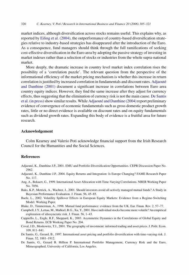
Here, n is either the number of national market indices or of stocks. In Fig. 1, we plotthe monthly average correlation amongst the country indexes and the individual stocks. Theformer has been computed applying (1) and (2) to our country index data with n = 5. Thisseries shows a strong tendency to rise over time. The average stock correlation series hasbeen computed applying (1) and (2) to our stock data with n = 42. This series does not show

Fig. 1. Average market index and stock correlations. Note: This figure plots the unconditional estimates of theaverage correlation between the 5 largest stock market indices in the Euro area and the average correlation between42 stocks included in the Eurostoxx50 Index over the sample period.


Table 3Unit root, specification and Wald-type tests

CV DF ADF1 ADF2 F-Test

Panel A (unit root tests on aggregate correlations)Country indexes

Intercept, no trend −2.89 −4.95 −4.10 −2.67 620.01Intercept and linear trend −3.45 −7.62 −7.46 −5.57 (0.000)

Individual stocksIntercept, no trend −2.89 −5.68 −4.07 −3.30Intercept and linear trend −3.45 −5.65 −4.04 −3.28

Static model Dynamic model

DW-statistics α (percent)(t-statistics)

δ (percent)(t-statistics)

β (t-statistics) h-statistics(significance)

Wald-statistics(significance)

Panel B (specification and Wald-type tests)-3.28Country indexes

1.41 38.40 (7.09) 0.1937 (5.24) 0.29 (3.04) 5.08 (0.02) 27.40 (0.00)

Individual stocks0.96 16.66 (4.07) −0.0076 (0.22) 0.51 (5.95) 2.60 (0.10) 0.05 (0.82)

Note: Panel A of this table reports Dickey–Fuller (DF) tests and augmented Dickey–Fuller (ADF1 and ADF2, thenumbers denoting the order of augmentation) tests for the presence of unit roots in the average country and stockunconditional correlations series. CV denotes the critical value at the 5 percent level. All variables are definedin the text. F-test denotes critical value and significance level (in brackets) of the test statistic under the null thatthe trend coefficient is zero and the series contains a unit root. Panel B reports estimates of the parameters ofthe model of the average country and stock correlations series with a deterministic time trend. DW denotes theDurbin–Watson statistics of the static model. All other columns report estimated coefficient and t-statistics forthe dynamic model. The rightmost columns report the Durbin’s h-statistic of the null that the dynamic modelresiduals are not first-order autocorrelated and the Wald statistic (in both cases with the associated significancelevels) of the restriction that δ is equal to zero. All the Wald-Test statistics, standard errors and significance levelshave been computed using a Newy–West adjusted variance–covariance matrix with Parzen weights to correct forheteroscedasticity and autocorrelation. All variables are defined in the text.Static model: yt = α + δt + ut, ut ∼ i.i.d.N(0, σ2).Dynamic model: yt = α + βyt−1 + δt + ut, ut ∼ i.i.d. N(0, σ2).

any strong tendency to rise over time but rather appears very noisy and persistent. It takesa substantial amount of time to revert to a fairly stable long run mean (in the region of 20percent) around which it oscillates.

3.1. Unit root tests

To test for the presence of a stochastic time trend, we conduct Dickey–Fuller (DF)and augmented Dickey–Fuller (ADF) tests allowing for up to 12 lags. As pointed out byPesaran and Pesaran (1997), however, there is a size-power trade-off depending on the orderof augmentation, and we consequently rely on the results provided by the tests performedat the lower orders of augmentation. As reported in Panel A of Table 3, the DF and ADFtests reject the null of a unit root at the 5 percent level of significance for average stockcorrelation. For the average correlation amongst the five Euro area stock market indexes,we cannot reject the null of a unit-root in the ADF test with two orders of augmentation


and no deterministic time trend. However, using an F-test and the appropriate non-standardasymptotic distribution (Hamilton, 1994), we can reject at the 1 percent level the jointhypothesis that the deterministic time trend is equal to zero and that there is a unit root. Wetherefore conclude that both correlation series are stationary and, in particular, aggregatemarket index correlation is trend-stationary.

3.2. Wald-type tests

To check on the possible presence of a deterministic time-trend, we regress our con-structed average correlations series on the latter. However, the residuals of a static modelthat includes among the regressors only a constant and a deterministic time-trend are auto-correlated, as suggested by the Durbin–Watson (DW) statistic. We therefore estimate adynamic model that also includes the first lag of the dependent variable. We then conductWald-type tests of the restriction that the deterministic time trend coefficient is zero usingNewy–West adjusted variance–covariance matrices to correct for heteroschedasticity andautocorrelation. Panel B of Table 4 presents the results. The time trend coefficient is largeand significant only for average country index correlation. It explains an increase in thelatter of about 2.5 percent per year. However, the Durbin’s h-statistic4 suggests that theresiduals are not serially independent. Therefore, we treat this trend coefficient estimatewith caution.

4. Conditional correlations

Thus far, we have applied an unconditional estimation methodology. This strategy hasyielded useful insights but it has the main shortcomings that, while the average of squares andcross-products are consistent estimators of the second moments of the return distributions,they might be biased in small samples since they are ad hoc representations of the volatilityand correlation processes. Moreover, the aggregation of daily data into lower frequencymonthly data leads to a potential small sample problem. It is therefore of considerableinterest to apply the recently developed DCC-MVGARCH model of Engle (2001, 2002)and Engle and Sheppard (2001). This provides a useful way to describe the evolution overtime of the second moments of large systems. In particular, we use the specification of theasymmetric DCC-MVGARCH proposed by Cappiello et al., (2003) and extend it to includea deterministic time trend:

Rt = const + ut

ut|�t−1 ∼ Φ(0, Ht)(3)

4 In the presence of lagged values of the dependent variables the DW test is biased toward acceptance of thenull of no error auto-correlation. We therefore test for serial correlation of the error terms using Durbin’s (1970)h-test. We use the generalised version of this test, developed by Godfrey and Breusch, based on a general LagrangeMultiplier test. Even though this procedure can detect higher order serial correlation, we only test the null of nofirst-order residual autocorrelation.


Table 4ADCC-MVGARCH country correlation

Panel A

Model Restriction Coefficient Coefficient estimate T-ratio p-Value

1 Q1 = Q2 Q1/2 0.799θ = 0 α 0.010 4.50 0.000

β 0.982 180.97 0.000δTrend 0.000 2.03 0.041

2 Q1 = Q2 Q1/2 0.799θ = 0 α 0.010 4.55 0.000δtrend = 0 β 0.985 223.82 0.000

3 Q1 = Q2 Q1/2 0.799θ = 0 α 0.007 12.72 0.000δtrend = 0 β 0.993 1807.09 0.000α + β = 1

4 θ = 0 Q1 0.611δtrend = 0 Q2 0.908

α 0.002 8.30 0.000β 0.970 589.68 0.000

5 δtrend = 0 Q1 0.611Q2 0.908α 0.002 3.90 0.000β 0.590 74.31 0.000θ 0.090 7.69 0.000

Panel B

Unrestricted model ln(|ΣUR|) Restrictedmodel

ln(|ΣR|) LR Statistic SignificanceLevel

RestrictionRejection

2 −5.0689 3 −5.0798 33.19 0.000 Yes4 −5.0665 2 −5.0689 25.15 0.020 Yes5 −5.0654 4 −5.0665 2.53 0.112 NoLR = T [ln(|ΣUR|) − ln(|ΣR|)] ∼ χ2(1)T = number of observations (2297)ΣUR = covariance matrix of the residuals of the unrestricted modelΣR = covariance matrix of the residuals of the restricted modelχ2(1) = Chi-Squared distributions with 1 degree of freedom

Note: Panel A of this table reports coefficients, t-statistics and p-values for various specifications of the ADCC-MVGARCH model of conditional correlations amongst the five largest Euro-zone market indexes. Panel B reportslikelihood ratio (LR) test statistics and their significance level.

where

Ht ≡ DtCtDt (4)

D2t = D2(1 − A − B) + A(ut−1u

′t−1) + BD2

t−1 (5)

Ct = C (1 − α − β) − Sθ − t(ii′ − I)δtrend + αεt−1ε′t−1 + βCt−1

+θSt−1 + δtrendt(ii′ − I) (6)


Here, ut is an nx1 vector of zero mean innovations conditional on the information setavailable at time t−1 (�t−1). They follow a Φ distribution, not necessarily normal, withcentred second moment matrix Ht. Also, Dt is the diagonal matrix of conditional standarddeviations and Ct is the conditional correlation matrix. Both Dt and Ct and, as a consequence,Ht are assumed to be positive definite. Also, D, A and B are nxn diagonal non-negativecoefficient matrices, C and S are positive definite coefficient matrices, θ, α, β and δtrend arescalar coefficients, i is a unit vector, I is a conformable identity matrix, t is a time trend,the elements of the nxn matrix St−1 are the outer-products of two vectors that contain onlynegative return innovations. To complete the notation, C takes the value Q1 if t < τ and Q2if t > τ, where τ represents a selected structural break date. Similarly, S takes the value N1if t < τ and the value N2 if t > τ, t is the mid point of the sample period (the unconditionalsample average of the values taken by the time trend variable).

To see why the inclusion of the deterministic time trend requires this specification,consider for simplicity but without loss of generality the univariate case of a GARCH(1,1) with deterministic time trend, Et−1(ε2

t ) = γ + αε2t−1 + βEt−2(ε2

t−1) + δtrendt. Takingunconditional expectations and using the law of iterated expectations, the unconditionalvariance is:

E(ε2t ) = γ + (α + β)E(ε2

t−1) + δtrendE(t) = γ + (α + β)E(ε2) + δtrend t (7)

Therefore, E(ε2t ) = (γ + δtrend t)/(1 − α − β) and γ = E(ε2

t )(1 − α − β) − δtrend t. Thespecification in (6) is a generalization to the multivariate case of this result.

The elements along the main diagonal of the matrix D can be seen as the long-run, baseline levels to which conditional variances mean-revert. The matrices C and S

can be seen as the long-run, baseline levels to which the conditional correlations of thereturn innovations and of the negative return innovations respectively mean-revert5. Tohasten the estimation procedure, D and C can be set equal to the unconditional vari-ance and correlation matrix over the sample, Q1 and Q2 can be set equal to the sampleaverage of εt−1ε

′t−1 before and after the date τ, and N1 and N2 are the sample aver-

age of St−1 before and after τ (in this case, the estimated conditional correlation matrixis not guaranteed to be positive-definite). When the coefficient θ is not constrained tobe zero, the correlation process can be asymmetric. A symmetric DCC model giveshigher tail dependence for both upper and lower tails of the multi-period joint density.An asymmetric DCC gives higher tail dependence in the lower tail of the multi-perioddensity.

Engle (2001, 2002) and Engle and Sheppard (2001) propose maximising the log-likelihood function of (3) in two steps to overcome the well-known computational problemsof MVGARCH models. They first maximise the log-likelihood with respect to the param-eters that govern the process of Dt. This can be done by estimating univariate models6 ofthe returns on each stock nested within a univariate GARCH model of their conditionalvariance. They then suggest maximising the second part of the likelihood function over the

5 I estimate this using the sample average of the negative return innovation cross-products.6 The presence of an intercept term ensures that the estimated residuals are zero-mean random variables.


parameters of the process of Ct, conditional on the estimated Dt. Preliminarily, this entailsstandardising ut by the estimated Dt to obtain the nx1 vector ε7

t . Engle (2001, 2002) andEngle and Sheppard (2001) show that this two-stage procedure yields consistent maximumlikelihood parameter estimates, and that the inefficiency in the two-stage estimation pro-cess can be taken into account by modifying the asymptotic covariance of the correlationestimation parameters.

Table 4 presents our ADCC-MVGARCH model quasi-maximum likelihood estimatesusing daily data on the five market indices. We first estimate a simple restricted symmetricspecification of (6) with a deterministic time trend but no structural break. We label thisspecification Model 1. The estimated deterministic time trend coefficient turns out to bestatistically significant but very small. Since it is economically negligible, we drop it fromall subsequent specifications. We therefore estimate Model 2, which imposes on Model 1the restriction that the time trend coefficient is zero.

Considering the clear rise in average market index correlation visible in Fig. 1, togetherwith the lack of evidence of a significant deterministic time trend, we then test for thepresence of either a stochastic trend or a structural break. To check the stationarity ofthe correlation process, we test the restriction that the news and persistence parameters α

and β sum to unity. The relevant LR test statistic and the associated significance level arereported at the bottom of Table 4 (Model 2 against Model 3). We reject the restriction thatthe parameters of the correlation process sum to unity and we conclude, therefore, that thecorrelation process is stationary.

A structural break in the market index correlation process might, however, explain boththe strong persistence of the series and its sharp increase over the sample period. In order toidentify the structural break date, we seek guidance from Government bond yields7. The plotof the likelihood of an ADCC-GARCH model of the Government bond index returns as afunction of 30 successive structural break dates, as reported in Fig. 2, peaks at the beginningof 1998. We also experimented with various possible structural break dates directly in thecorrelations process of the stock market indices. The model with a structural break datein January 1998 displays again the largest likelihood8. This hypothesis about the timingof the structural break occurrence is intuitively appealing since it is roughly 12 monthsbefore the official introduction of the Euro and thus it accounts for the likely possibilitythat financial markets started to discount it in the price formation mechanism somewhat inadvance.

Therefore, we finally settled on the beginning of January 1998, as this date maximisethe likelihood of a ADCC-GARCH model of the bond index returns, it almost exactlysplits our sample in half and allows for the possibility that stock markets discount ratesmight have reflected the expectation of monetary policy convergence and increased finan-cial integration prior to the introduction of the new currency. Using the usual LR test

7 A necessary condition for the parity of expected real rates of returns is that bond yields differentials reflectinflation differentials. Under this perspective and neglecting differences in risk premia across countries, a structuralbreak in Euro area interest rates correlations due to monetary policy convergence is a likely cause for a structuralbreak in correlations at the stock market index level. This is also suggested, for example, by the study of Cappielloet al. (2003) and of Hardouvelis et al. (2000).

8 Results for the other models are not reported to save space (they are a long list of structural break dates andcorresponding likelihood function values) but they are available upon request.


Fig. 2. Euro area government bond yields log-likelihoods and LR statistics with rolling structural break dates.Note: Panel A plots the likelihood of an ADCC-GARCH model of the bond index returns as a function of 30successive structural break dates. Panel B reports the Chi-Squared statistic of the corresponding LR test. Thisstatistic is significant at the 5 percent level for structural break dates from 1994 to 2000.The restricted model inthe LR test is the model with no structural break date.

statistic, reported at the bottom of Table 5, we therefore tests Model 4 that allows for astructural break in 1998 against Model 2, the restricted model with no structural break.We can reject this restriction at the 0.020 significance level. Moreover, once we allow forthe structural break, the restriction that the asymmetric component coefficient θ is equalto zero (Model 5 against Model 4) cannot be rejected at the 5 percent level. The coeffi-cient θ is only marginally significant. Its size however is non negligible from an economicpoint of view. In particular, its point estimate is 45 times as large as the news reactionparameter α.

We therefore conclude that the aggregate correlation between the five Euro-zone stockmarket indices and the Eurostoxx50 index is best explained by a DCC-GARCH processwith a structural break in its mean9 and, perhaps, an asymmetric reaction component. Fig. 3

9 We also estimated each model with the Eurostoxx50 index, and over the longer sample period 1992–2002,excluding the MIB30 index (because its series starts a year later). We obtained very similar results in all cases,and these are not reported here for brevity.


Table 5ADCC-MVGARCH 42 Eurostoxx50 stocks

Panel A

Model Restriction Coefficient Coefficient estimate T-ratio p-Value

1 Q1 = Q2 α 0.002 16.51 0.000δtrend = 0 β 0.989 1222.29 0.000θ = 0

2 Q1 = Q2 α 0.002 15.06 0.000δtrend = 0 β 0.989 1214.20 0.000

θ 0.001 1.55 0.121

Panel B

Unrestricted model ln(|ΣUR|) Restrictedmodel

ln(|ΣR|) LR statistic Significancelevel

Restrictionrejection

2 −13.6466 1 −13.6474 1.7486 0.186 NoLR = T ln(|ΣUR|) − ln(|ΣR|) ∼ χ2(q)T = number of observations (2289)ΣUR = covariance matrix of the residuals of the unrestricted modelΣR = covariance matrix of the residuals of the restricted modelχ2(q) = Chi-Squared distributions with q degrees of freedomq = number of restrictions (q = 1)

Note: Panel A of this table reports the coefficients, t-statistics and p-values for the ADCC-MVGARCH modelof conditional correlations amongst 42 stocks (k = 42) included in the Eurostoxx50 index. The data frequency isdaily. Variables and their coefficients are defined in the text. Panel B reports likelihood ratio (LR) test statisticsand their significance level.

plots the market index average conditional correlation estimated with the symmetric Model5, allowing for a structural break in 1998.

Turning to the correlation patterns at a more disaggregated level, the estimation resultsfor the 42 individual stocks are shown in Table 5. The estimated θ is very small and the

Fig. 3. DCC-MVGARCH Country Correlation. Notes: This figure plots the daily average conditional correlationamongst the five Euro-zone market, estimated with the symmetric DCC-MVGARCH(1, 1) model with a structuralbreak at the beginning of 1998.


Fig. 4. DCC-MVGARCH stock correlations. Notes: This figure plots the daily average conditional correla-tion amongst 42 individual stocks included in the Eurostoxx50 index, estimated with the symmetric DCC-MVGARCH(1, 1).

restriction that it is equal to zero10 cannot be rejected at any conventional significance level.The time series of the estimated symmetric average conditional industry, sector and stockreturn correlation is plotted in Fig. 4. The plot for the asymmetric case is almost identical.

As a specification check, we apply the Engle and Ng (1993) test in a multivariate settingto our country-level MV-ADCC and MV-DCC GARCH models. Originally, this test wasdesigned as a diagnostic check for univariate volatility models and its aim is to examinewhether there is residual predictability in squared standardised conditional errors usingsome variables observed in the past which are not included in the volatility model. Sincemultivariate variance–covariance models provide estimates of all the ingredients that areneeded to compute the conditional portfolio volatility if asset weights are known, we canuse our first and second step MV-ADCC and MV-DCC GARCH conditional volatility andcorrelation estimates to compute the conditional volatility and the conditional residuals ofan equally weighted portfolio. We can then apply the Engle and Ng (1993) test to returnson the latter.

In particular, we apply a test that combines the Sign Bias test (that uses as regressorsdummy variables I− that take value 1 or 0 depending on weather the lagged residual isnegative or positive) and the negative and positive size bias test (that use, respectively, laggednegative and positive standardised residuals as regressors, z−

t−1 and z+t−1). As reported in

Table 6, we can reject the null of non-predictability of the squared standardised conditionalresiduals. Therefore, in spite of the mixed evidence provided by the LR tests of the ADCC-MVGARCH against the DCC-MVGARCH, distributional asymmetric are important. Thelatter are probably of a non-linear nature11 and we leave the difficult quest for a betterspecification for future research.

10 We do not report estimates with a deterministic time trend because the estimation procedure did not converge.11 This, as far market indices are concerned, lies in partial contrast to those reported by Cappiello et al. (2003).

However, since we were able to replicate their results with their same set of market indices, frequency and dataperiod (these results are not reported for brevity and because they exactly match results already published byCappiello et al. (2003) but they are available upon request), we conclude that the difference between our and


Table 6Diagnostic tests

Model DCCa

S− [significance] 0.68 [0.394]a

u− [significance] −0.123 [0.039]a

u+ [significance] −0.142 [0.058]a

Chi- squared (3) [significance] 29.64 [0.000]a

Notes: This table reports the coefficients and p-values for a multivariate application of the Engle and Ng (1993)test. Variables and their coefficients are defined in the text.

a Country indices—daily

5. Summary and conclusions

The purpose of this paper is to contribute to the literature on the correlation dynamicsin European equity markets. Our main focus has been on country-level market index corre-lations, but we also examined stock correlations for comparison purposes. We applied thesymmetric and asymmetric version of the DCC-MVGARCH model of Engle (2001, 2002)and Engle and Sheppard (2001) to capture their behaviour over time.

We find strong evidence of a structural break in the mean shortly before the introductionof the Euro. This explains both the strong persistence of the correlation time series and itssignificant rise over the sample period. This confirms the results reported by Cappiello etal. (2003) and is consistent with the rise in volatility spillovers noticed by Baele (2002).We also find evidence that, at the level of the national stock market indices, the conditionalcorrelation response to past positive and negative news is asymmetrical. Stock correlationsinstead do not appear to follow an asymmetric correlation process. These findings providemixed support to a popular explanation see, for example, Patton (2002) for why the skewnessof market index returns is often negative whereas stock returns have either negative orpositive skewness (similar findings are reported in Table 2). More importantly, applying amultivariate extension of the Engle and Ng (1993) test, we find that beyond asymmetriccorrelation reactions to past returns innovations there must be other, perhaps more importantsource of asymmetry in the distribution of asset returns. This issue represents an importantand fruitful topic for future research.

Overall, our results suggest that non-country factors drive the volatility of equity returns.In particular, because of the rise in correlations among the largest national stock marketsindices, the stochastic components of the latter can now be expected to behave almost iden-tically (with conditional correlations being close to 100 percent as reported in Fig. 3). Thissuggests that there is little expected benefit from strategies that diversify across Euro-zone

their results is due to whether non-Euro area market indices are included. Correlations amongst Euro area marketindices, in particular, appear to display a substantial lower tendency to increase following joint past negative returnsthan those amongst markets outside the Euro area. Another likely but less important reason for why our resultsdiffer from those of Cappiello et al. (2003) with respect to the importance of asymmetric correlation reactions topast returns innovations is the different data frequency—they use only weekly data whereas we use both daily andweekly data and for the former the importance of the asymmetric correlation component is always lower. Thissuggests the importance of taking into account temporal aggregation issues when modelling asset returns secondmoments dynamics.


market indices, although diversification across stocks remains useful. This explains why, asreported by Eiling et al. (2004), the outperformance of country-based diversification strate-gies relative to industry-based strategies has disappeared after the introduction of the Euro.As a consequence, fund managers should think through the full ramifications of seekingcost-effective diversification in the Euro area by adopting the passive strategy of investing inmarket indexes rather than a selection of stocks or industries from the whole supra-nationalmarket.

More deeply, the dramatic increase in country level market index correlation rises thepossibility of a ‘correlation puzzle’. The relevant question from the perspective of theinformational efficiency of the market pricing mechanism is whether this increase in returncorrelation is justified by increased correlation in fundamentals and discount rates. Adjaouteand Danthine (2001) document a significant increase in correlations between Euro areacountry equity indices. However, they find the same increase after they adjust for currencyeffects, thus suggesting that the elimination of currency risk is not the main cause. De Santiset al. (in press) show similar results. While Adjaoute and Danthine (2004) report preliminaryevidence of convergence of economic fundamentals such as gross domestic product growthrates, little or no direct evidence is available on discount rates and on equity fundamentalssuch as dividend growth rates. Expanding this body of evidence is a fruitful area for futureresearch.

Acknowledgement

Colm Kearney and Valerio Poti acknowledge financial support from the Irish ResearchCouncil for the Humanities and the Social Sciences.

References

Adjaoute, K., Danthine J.P., 2001. EMU and Portfolio Diversification Opportunities. CEPR Discussion Paper No.2962.

Adjaoute, K., Danthine J.P., 2004. Equity Returns and Integration: Is Europe Changing? FAME Research PaperNo. 117.

Ang, A., Bekaert, G., 1999. International Asset Allocation with Time-Varying Correlations. NBER Working PaperNo. 7056.

Baks, K.P., Metrick, A., Wachter, J., 2001. Should investors avoid all actively managed mutual funds? A Study inBayesian Performance Evaluation. J. Finan. 56, 45–85.

Baele, L., 2002. Volatility Spillover Effects in European Equity Markets: Evidence from a Regime-SwitchingModel. Working Paper.

Blake, D., Timmerman, A., 1998. Mutual fund performance: evidence from the UK. Eur. Finan. Rev. 2, 57–77.Campbell, J.Y., Lettau, M., Malkiel, B.G., Xu, Y., 2001. Have individual stocks become more volatile? An empirical

exploration of idiosyncratic risk. J. Finan. 56, 1–43.Cappiello, L., Engle, R.F., Sheppard, K., 2003. Asymmetric Dynamics in the Correlations of Global Equity and

Bond Returns. ECB Working Paper No. 204.Coval, J.D., Moskowitz, T.J., 2001. The geography of investment: informed trading and asset prices. J. Polit. Econ.

109, 811–841.De Santis, G., Gerard, B., 1997. International asset pricing and portfolio diversification with time-varying risk. J.

Finan. 52, 1881–1912.De Santis, G., Gerard B. Hillion P. International Portfolio Management, Currency Risk and the Euro,

Mimeographed, University of California, Los Angeles.


Durbin, J., 1970. Testing for serial correlation in least squares regression when some of the regressors are laggeddependent variables. Econometrica 38, 410–421.

Eiling, E., Gerard, B., de Roon F., 2004. Asset Allocation in the Euro-Zone: Industry or Country Based?Mimeographed.

Engle, R.F., 2001. Dynamic Conditional Correlation—A Simple Class of Multivariate Garch Models. WorkingPaper, University of California, San Diego.

Engle, R.F., 2002. Dynamic conditional correlation: a simple class of multivariate generalised autoregressiveconditional heteroskedasticity models. J. Bus. Econ. Stat. 20, 339–350.

Engle, R.F., Ng, V.K., 1993. Measuring and testing the impact of news on volatility. J. Finan. 48, 1749–1777.Engle, R.F., Sheppard, K., 2001. Theoretical and Empirical Properties of Dynamic Conditional Correlation Mul-

tivariate GARCH. Working Paper, University of California, San Diego.Erb, C.B., Harvey, C.R., Viskanta, T.E., 1994. Forecasting international equity correlations. Finan. Anal. J. 50,

32–45.Fratzschler, M., 2002. Financial market integration in europe: on the effects of Euro area on stock markets. Int. J.

Finan. Econ. 7, 165–193.Hamilton, J.D., 1994. Time Series Analysis. Princeton University Press, Princeton.Hardouvelis, G., Malliaropulos, D., Priestley, R., 2000. Euro area and European Stock Market Integration. CEPR

Discussion Paper.Longin, F., Solnik, B., 1995. Is correlation in international equity returns constant: 1960–1990? J. Int. Money

Finan. 14, 3–26.Longin, F., Solnik, B., 2001. Extreme correlation of international equity markets. J. Finan. 56, 649–676.Merton, R.C., 1980. On estimating the expected return on the market: an exploratory investigation. J. Finan. Econ.

8, 323–361.Patton, A. J., 2002. Skewness, Asymmetric Dependence and Portfolios. Working Paper, University of California,

San Diego.Pesaran, M.H., Pesaran, B., 1997. Working with Microfit 4.0. Oxford University Press, Oxford.Wermers, R., 2000. Mutual fund performance: an empirical decomposition into stock-picking talent, style, trans-

action costs, and expenses. J. Finan. 55, 1655–1695.

Documents

Correlation dynamics in European equity markets