This paper can be downloaded without charge at:

The Fondazione Eni Enrico Mattei Note di Lavoro Series Index: http://www.feem.it/Feem/Pub/Publications/WPapers/default.htm

Social Science Research Network Electronic Paper Collection:

http://ssrn.com/abstract=1158446

The opinions expressed in this paper do not necessarily reflect the position of Fondazione Eni Enrico Mattei

Corso Magenta, 63, 20123 Milano (I), web site: www.feem.it, e-mail: working.papers@feem.it

Corruption, Income Inequality, and Poverty in the United States Oguzhan C. Dincer and Burak Gunalp

NOTA DI LAVORO 54.2008

JUNE 2008 KTHC – Knowledge, Technology, Human Capital

Oguzhan C. Dincer, Department of Economics Illinois State University Burak Gunalp, Department of Economics, Hacettepe University

Corruption, Income Inequality, and Poverty in the United States Summary In this study we analyze the effects of corruption on income inequality and poverty. Our analysis advances the existing literature in four ways. First, instead of using corruption indices assembled by various investment risk services, we use an objective measure of corruption: the number of public officials convicted in a state for crimes related to corruption. Second, we use all commonly used inequality and poverty measures including various Atkinson indexes, Gini index, standard deviation of the logarithms, relative mean deviation, coefficient of variation, and the poverty rate defined by the U.S. Census Bureau. Third, we minimize the problems which are likely to arise due to data incomparability by examining the differences in income inequality, and poverty across U.S. states. Finally, we exploit both time series and cross sectional variation in the data. We find robust evidence that an increase in corruption increases income inequality and poverty. Keywords: Corruption, Income Inequality, Poverty JEL Classification: D31, D73, I32

Address for correspondence: Oguzhan C. Dincer Department of Economics Illinois State University Campus Box 4200 Normal IL 61790 USA E-mail: odincer@ilstu.edu

3

Corruption, Income Inequality and Poverty in the United States

1. Introduction

An increasing number of empirical studies (e.g. Mauro 1995, Knack and Keefer

1995, Knack 1996, Keefer and Knack 1997, Mo 2001, Pellegrini and Gerlagh 2004)

present persuasive evidence regarding the detrimental effects of corruption on various

economic variables such as the growth rate of income.

Corruption does not only affect the growth rate of income but also affects income

inequality and poverty. “The benefits from corruption are likely to accrue to the better

connected individuals … who belong mostly to high income groups” (Gupta et. al. 2002,

23). According to Jonston (1989), corruption favors the ‘haves’ rather than the ‘have

nots’ particularly if the stakes are large. The burden of corruption falls disproportionately

on low income individuals. Individuals who belong to low income groups pay a higher

proportion of their income than the individuals who belong to high income groups. As

Tanzi (1998) argues, corruption distorts the redistributive role of government. Since only

the better connected individuals get the most profitable government projects, it is less

likely that the government is able to improve the distribution of income and make the

economic system more equitable. It diverts government spending away from projects that

benefit mostly low income individuals such as education and health to, for example,

defense projects that create opportunities for corruption (Chetwyn et al. 2003).

Nevertheless, there are only a few empirical studies (Li, Xu, and Zou 2000, Gupta et. al.

2002, and Chong and Calderon 2000a and 2000b) analyzing the effects of corruption on

income inequality and poverty. Using data from a mixed group of countries, i.e., low,

4

middle, and high-income, Li, Xu, and Zou (2000) and Chong and Calderon (2000a) find

an inverse U-shaped relationship between corruption and income inequality. They find a

positive relationship between corruption and income inequality in high-income countries

and a negative relationship in low-income countries. Gupta et al. (2002), on the other

hand, using a smaller sample of countries, find a positive and linear relationship between

corruption and income inequality. Chong and Calderon (2000b) and Gupta et al. (2002)

both analyze the effects of corruption on poverty as well as on income inequality. As

Chong and Calderon (2000b) argue, an increase in income inequality as corruption

increases does not necessarily mean that poverty also increases. If, for example, the

incomes in the higher end of the distribution grow faster than incomes in the lower end of

the distribution, income inequality increases while poverty decreases. Both Chong and

Calderon (2000b) and Gupta et al. (2002) find a positive and linear relationship between

corruption and poverty.

In this study, we analyze the effects of corruption on income inequality and

poverty by using data from U.S. states. Using data from U.S. states is quite advantageous.

The likelihood of the problems arising due to data incomparability is minimal. Data on

corruption as well as on income inequality and poverty for U.S. states are more

comparable than those for different countries, and U.S. states are more similar in other

dimensions that are difficult to measure. We find robust evidence that an increase in

corruption increases income inequality and poverty across U.S. states.

Our analysis advances the existing literature in three ways. First, instead of using

subjective cross-country corruption indices assembled by various investment risk

services, we use an objective measure of corruption: the number of government officials

5

convicted in a state for crimes related to corruption. Second, we employ all commonly

used inequality and poverty measures including various Atkinson indexes, Gini index,

standard deviation of the logarithms, relative mean deviation, coefficient of variation, and

the poverty rate defined by the U.S. Census Bureau. Finally, we exploit both time series

and cross-sectional variation in the data.

2. Data

We use annual data from 50 states for 17 years, from 1981 to 1997. For our

measure of corruption (Corruption), we use the number of government officials

convicted in a state for crimes related to corruption in a year. The data are from the

Justice Department’s “Report to Congress on the Activities and Operations of the Public

Integrity Section”. These data are used by several studies such as Goel and Rich (1989),

Fisman and Gatti (2002), Fredriksson, List and Millimet (2003) and Glaeser and Saks

(2006) to measure corruption across states. They cover a broad range of crimes from

election fraud to wire fraud. We deflate the number of convictions by state population.

As Glaeser and Saks (2006) argue, using the number of convictions creates a problem

since a smaller number of government officials are likely to be convicted in corrupt

states. Following Glaeser and Saks (2006), to mitigate this problem, we focus on federal

convictions.

We measure income inequality across states by using the four traditional

measures Gini Index (Gini), standard deviation of the logarithms (SDL), relative mean

deviation (RMD), and the coefficient of variation (CV) as well as the various Atkinson

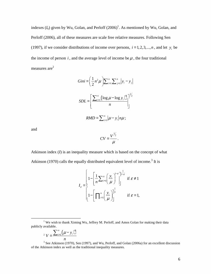
6

indexes (Iε) given by Wu, Golan, and Perloff (2006)1. As mentioned by Wu, Golan, and

Perloff (2006), all of these measures are scale free relative measures. Following Sen

(1997), if we consider distributions of income over persons, 1,2,3,...,i n= , and let iy be

the income of person i , and the average level of income beµ , the four traditional

measures are2

2

1 1

1

2

n n

i ji jGini n y yµ

= =

= −

∑ ∑

( )122

1log log

n

iiy

SDLn

µ=

− =

∑

1

n

iiRMD y nµ µ

== −∑ ;

and

12V

CVµ

= .

Atkinson index (I) is an inequality measure which is based on the concept of what

Atkinson (1970) calls the equally distributed equivalent level of income.3 It is

11 1

1

1

1

11 if 1

1 if 1,

n i

i

nn i

i

y

nI

y

ε ε

ε

εµ

εµ

− −

=

=

− ≠

=

− =

∑

∏

1 We wish to thank Ximing Wu, Jeffrey M. Perloff, and Amos Golan for making their data

publicly available.

2 ( )2

1

n

iiy

Vn

µ=

−= ∑

3 See Atkinson (1970), Sen (1997), and Wu, Perloff, and Golan (2006a) for an excellent discussion of the Atkinson index as well as the traditional inequality measures.

7

where, ε measures the degree of inequality aversion. It takes values ranging from 0 to

.∞ As ε increases the Atkinson index becomes more sensitive to changes at the lower

end of the income distribution and as ε decreases it becomes more sensitive to changes

at the higher end of the distribution. The index equals zero when distribution of income is

equal and approaches 1 as inequality increases. We assume ε is equal to 0.5, 1, and 1.5.4

We measure poverty by the percentage of people whose income is under the poverty

threshold given by the Census Bureau. In order to determine the number of people who

are in poverty, the Census Bureau uses a set of income thresholds that vary by the size

and the composition of the family. If a family’s total income is less than the family’s

threshold, then every person belonging to that family is considered in poverty. The

poverty thresholds are updated using the consumer price index.

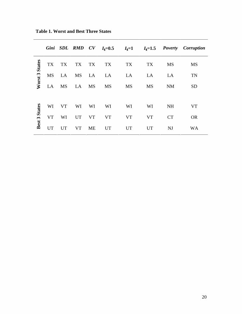
Based on the averages across the 17 years, Texas has the highest inequality

regardless of which inequality measure is used while Mississippi has the highest poverty.

Vermont has the lowest inequality when SDL is used to measure inequality while

Wisconsin has the lowest inequality when other measures are used. New Hampshire has

the lowest poverty. Mississippi and Vermont are the most and the least corrupt states,

respectively. The states with the three lowest and highest inequality and poverty as well

those with the three lowest and highest corruption are given in Table 1. The summary

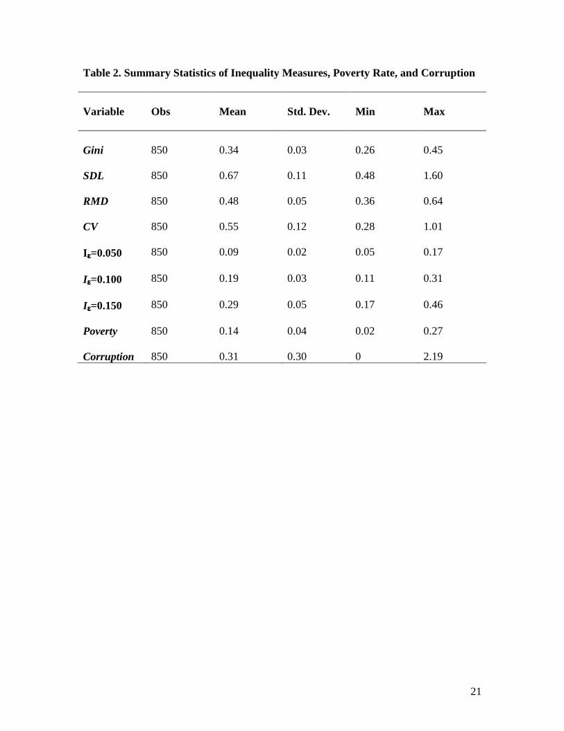
statistics for all of the inequality measures, poverty, and corruption are given in Table 2.

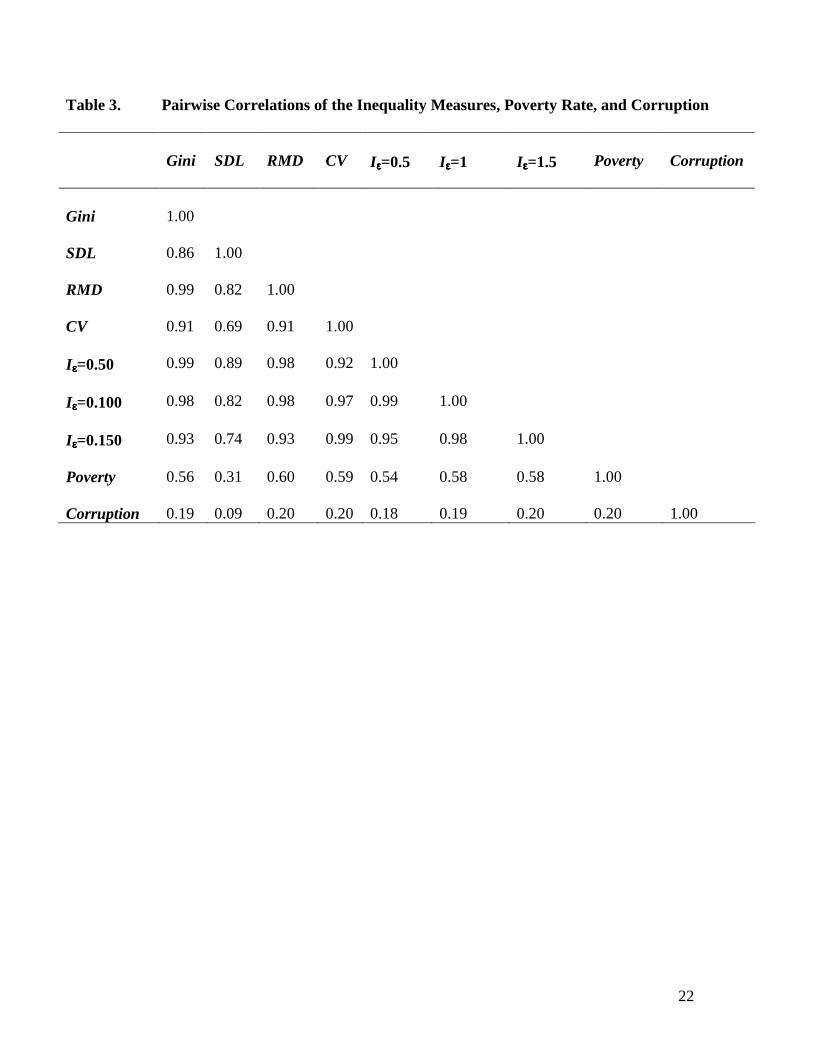
As expected, the correlations between the inequality measures, poverty, and

corruption are positive: the correlation coefficients between corruption and the inequality

measures are around 0.20 as is the correlation coefficient between corruption and

4 Atkinson (1970) assumes ε lies within the range of (0, 2.5]. The index is given for 0.1, 0.5, 1,

1.5, 2, and 2.5 by Wu, Perloff, and Golan (2006a). Nevertheless, to save space we do not report the results for 0.1, 2, and 2.5.

8

poverty. Pairwise correlations of the inequality measures, poverty, and corruption are

given in Table 3.

We include a set of control variables in our regressions to minimize the omitted

variable bias. First, following Wu, Perloff, and Golan (2006), we include a set of

government policy variables: earned income tax credit benefit rate (EITCB), earned

income tax credit phase-out rate (EITCP), and aid to the families with dependent

children/temporary assistance to needy families (AFDC/TANF). The AFDC/TANF is the

maximum monthly benefits for a single parent, three person family. EITCB is the product

of the earned income tax credit rate and the maximum income required for maximum

benefit. The earned income tax credit is phased out as a family's income rises. EITCP is

the rate at which the earned income tax credit benefit is reduced over the phase-out range.

The data are from Wu, Perloff, and Golan (2006). Second, we include two

macroeconomic variables: real per capita personal income (Income) and the

unemployment rate (Unemployment). The income data are from the Bureau of Economic

Analysis (BEA) and the unemployment data are from Bureau of Labor Statistics (BLS).

As Glaeser (2005) argues, stronger unions generally mean increased equality. Hence we

include the unionization rate (Union) as another control variable using the estimates

provided by Hirsch, Macpherson, and Vroman (2001). Finally, we include education

(Education) as our last control variable. We measure education as the share of secondary

school enrolment in the population. The data are from National Center for Education

Statistics.

9

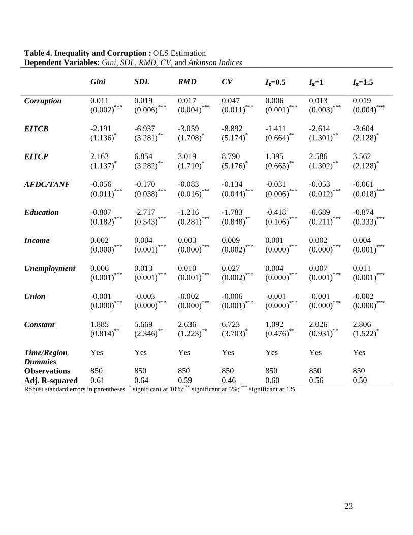
3. Results

Corruption and income inequality

To analyze the relationship between corruption and income inequality, we

estimate the following basic model by ordinary least squares (OLS) controlling for time

and region fixed effects:

st st st t s stInequality Corruption X T R uα β γ µ φ= + ⋅ + ⋅ + ⋅ + ⋅ +

where stInequality represents each of our measures of income inequality in state s during

period t. stCorruption represents corruption whereas Xst represents the set of control

variables that affect income inequality (EITCB, EITCP, AFDC/TANF, Education,

Income, Unemployment, Union), tT represents the set of year dummies, sR represents the

set of region dummies and stu represents the error term. The results of OLS estimation

are given in Table 4. The R2 ranges from 0.46 to 0.64. In all regressions, the estimated

coefficient of corruption is positive and highly significant indicating that corruption

increases income inequality. One standard deviation increase in Corruption increases

Gini, for example, by 0.3 percentage points, the same increase in Gini due to a 20 percent

decrease in AFDC/TANF. Up to 6 percent of the difference in Gini index between the

least corrupt state Vermont and the most corrupt state Mississippi is explained by

different corruption levels in those states. Similarly, one standard deviation increase in

Corruption increases SDL by 0.6 percentage points, RMD by 0.5 percentage points, and

CV by 1.4 percentage points.

As mentioned earlier, asε increases, the Atkinson index becomes more sensitive

to changes at the lower end of the income distribution. The estimated coefficient of

10

Corruption increases as ε increases, indicating that effects of corruption on the lower

end of the distribution are higher. One standard deviation increase in Corruption

increases Iε=0.5, Iε=1, and Iε=1.5, by 0.2, 0.4, and 0.6 percentage points, respectively.

Our results about the effects of macroeconomic and demographic control

variables on income inequality are mostly consistent with the earlier studies. The

estimated coefficients of Unemployment, Income, Education, and Union are significant in

all estimations. We find that education and unionization have an equalizing effect while

unemployment rate tends to increase income inequality as expected (Li et. al. 2000,

Gupta et. al. 2002, Glaeser 2005, Wu, Perloff, and Golan 2006). According to our

estimations, an increase in real per capita income increases income inequality. Regarding

the government policy variables, the estimated coefficients of EITCB, EITCP,

AFDC/TANF are significant in all estimations. Again, as expected, while the estimated

coefficient of EITCP is positive, the estimated coefficients of both EITCB and

AFDC/TANF are negative (Wu, Perloff, and Golan 2006).

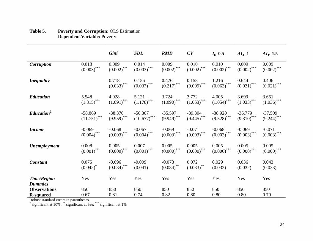
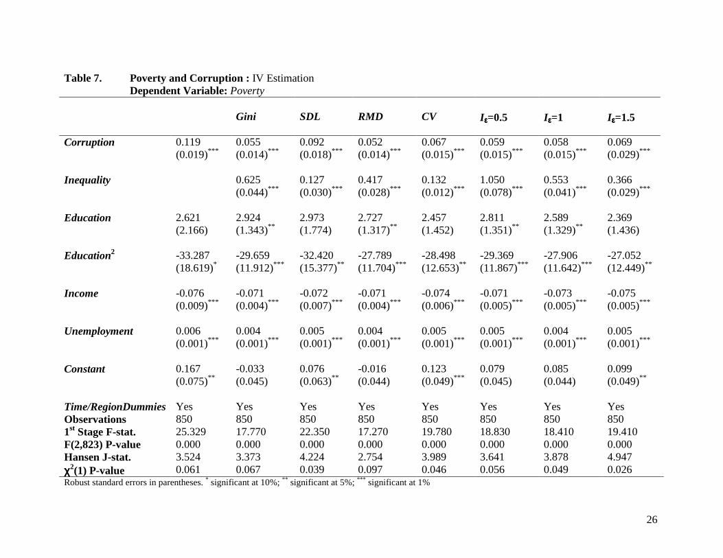
Corruption and poverty

In our poverty regressions we control for Income, Education, Unemployment,

region and year dummies, as well as inequality (Gini, SDL, RMD, CV, AI). The results of

the OLS estimation are given in Table 5.5 We first estimate a poverty regression without

controlling for inequality. The R2 is 0.67. The estimated coefficient of corruption is

positive and significant indicating that corruption increases poverty. One standard

deviation increase in Corruption increases Poverty by 0.5 percentage points, the same

5 In the second column we give the results of the regression in which we measure inequality by

Gini, third by SDL, fourth by RMD, fifth by CV, sixth by Iε=0.5, seventh by Iε=1, and eighth by Iε=1.5.

11

increase in Poverty due to a 10 percent increase in Unemployment. Up to 7 percent of the

difference in Poverty between Vermont and Mississippi is explained by different

corruption levels in those states. According to Ravallion (1997), income inequality

matters for poverty reduction. It is then quite likely that corruption affect poverty both

directly and indirectly through income inequality. In our regressions the coefficient of the

income inequality regardless of the measure we use is positive and highly significant

which is consistent with Chong and Calderon (2000b). When we include income

inequality in our poverty regressions the R2 increases significantly. It ranges from 0.74 to

0.82. In all regressions, the estimated coefficient of corruption is positive and highly

significant. Nevertheless the coefficient estimate decreases when we include inequality

indicating that corruption has indeed direct effects on poverty as well as indirect effects

through income inequality. Regarding the other control variables, we find a positive

relationship between Unemployment and Poverty and consistent with both Chong and

Calderon (2000b) and Gupta et al. (2002) a negative relationship between Income and

Poverty. According to our estimations, there is an inverse U-shaped relationship between

Education and Poverty.

4. Robustness of the Results

The main robustness issue is whether the results are due to reverse causality. As

You and Khagram (2005), Uslaner (2006), and Chong and Gradstein (2007) argue, high

income inequality and high poverty are likely to lead to more corruption. Instrumental

variables (IV) estimation helps address this problem. The choice of the instrument is

extremely important. A good instrument is a variable that is supposed to be uncorrelated

12

with the error term but correlated with the endogenous variable Corruption. Previous

studies such as Mauro (1995) use instruments such as ethnic fractionalization index

(EFI). The index is calculated as

11

P

s sppEFI n

== −∑ ,

where spn is the population share of group p in country s. EFI gives us the probability

that two randomly selected individuals in a country belong to two different ethnic groups.

It reaches a maximum if every individual in a country belongs to a different ethnic or

religious group. In our regressions we use both ethnic and religious fractionalization

indexes as our instruments. The data we use to calculate the EFI are from the Census

Bureau for 1970, which cover five ethnic groups: Whites, Blacks, American Indian and

Eskimos, Asians, and Others. The data we use to calculate the religious fractionalization

index (RFI) are from the American Religion Data Archive for the same year. These data

are collected by representatives of the Association of Statisticians of American Religious

Bodies to provide information on the number of churches and members for 53 Judeo-

Christian church bodies for 1971 representing an estimated 81 percent of church

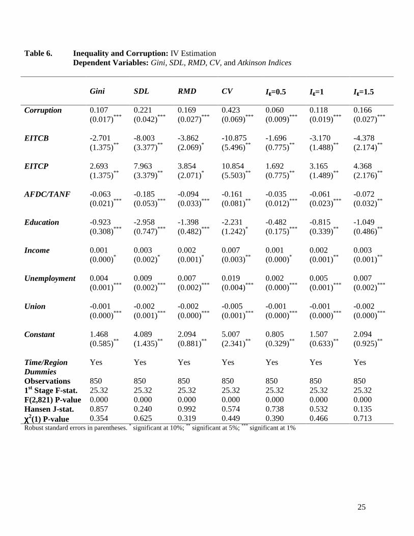
membership in the United States. The results of the IV estimation for the inequality

regressions are given in Table 6, and for the poverty regressions in Table 7. The

estimated coefficient of corruption is positive and highly significant in all regressions

indicating that our results are robust to reverse causality. As long as the ethnic and

religious fractionalization indexes affect income inequality and poverty through

Corruption, the instruments are theoretically valid. According to the 1st stage F and the

Hansen J statistics given in Table 6 and Table 7, they are empirically valid as well.

The second robustness issue is the possible measurement error in Corruption.

13

Nevertheless, IV estimation does not only help correct for reverse causality but also the

measurement error.

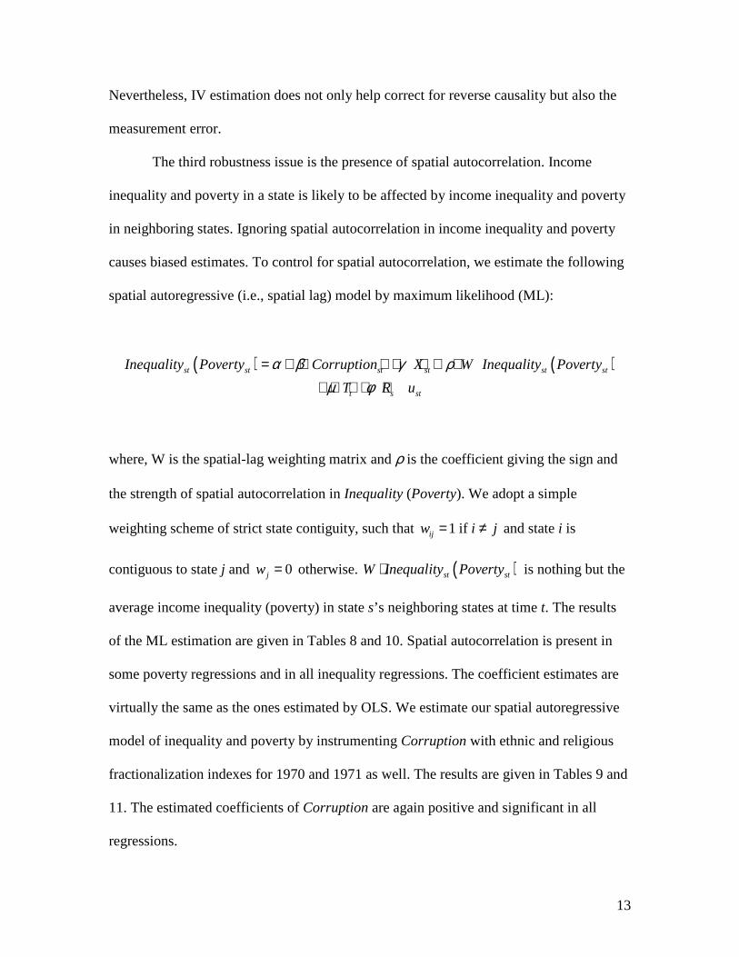
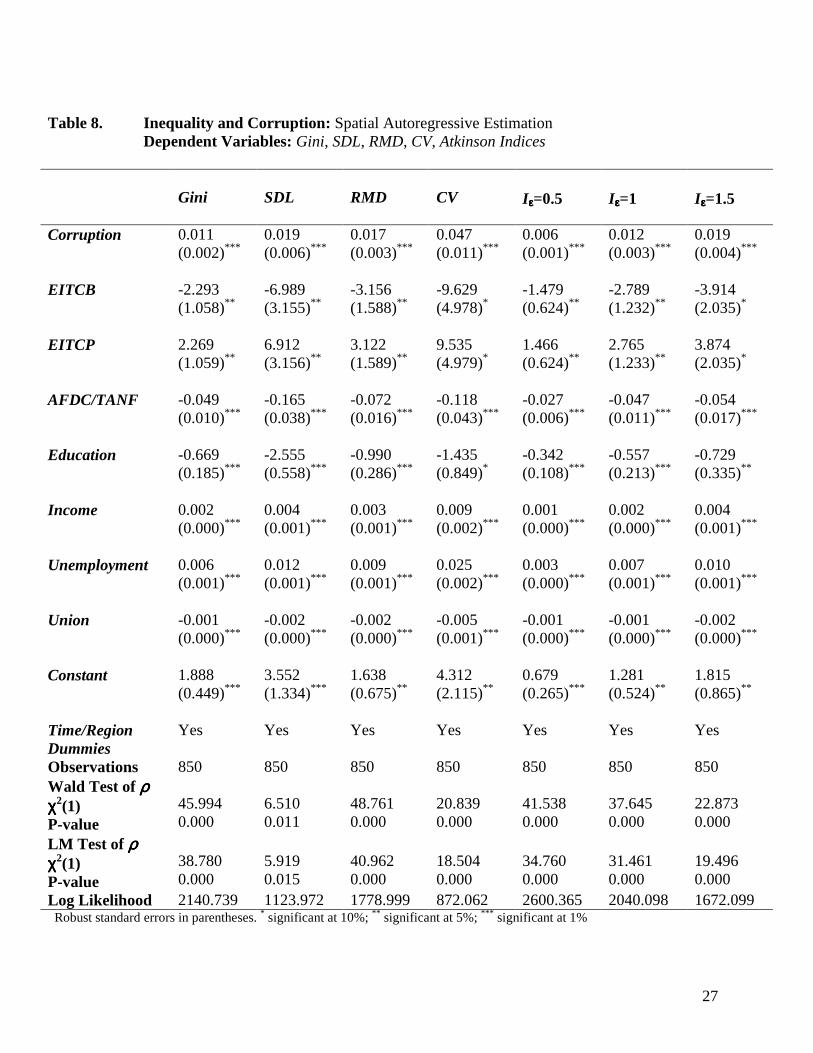
The third robustness issue is the presence of spatial autocorrelation. Income

inequality and poverty in a state is likely to be affected by income inequality and poverty

in neighboring states. Ignoring spatial autocorrelation in income inequality and poverty

causes biased estimates. To control for spatial autocorrelation, we estimate the following

spatial autoregressive (i.e., spatial lag) model by maximum likelihood (ML):

( ) ( )st st st st st st

t s st

Inequality Poverty Corruption X W Inequality Poverty

T R u

α β γ ρµ φ

= + ⋅ + ⋅ + ⋅ ⋅+ ⋅ + ⋅ +

where, W is the spatial-lag weighting matrix and ρ is the coefficient giving the sign and

the strength of spatial autocorrelation in Inequality (Poverty). We adopt a simple

weighting scheme of strict state contiguity, such that 1 if ijw i j= ≠ and state i is

contiguous to state j and 0jw = otherwise. ( )st stW Inequality Poverty⋅ is nothing but the

average income inequality (poverty) in state s’s neighboring states at time t. The results

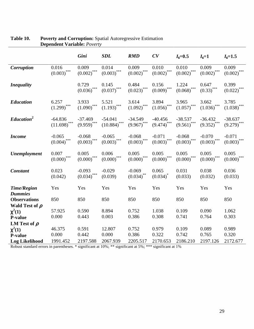
of the ML estimation are given in Tables 8 and 10. Spatial autocorrelation is present in

some poverty regressions and in all inequality regressions. The coefficient estimates are

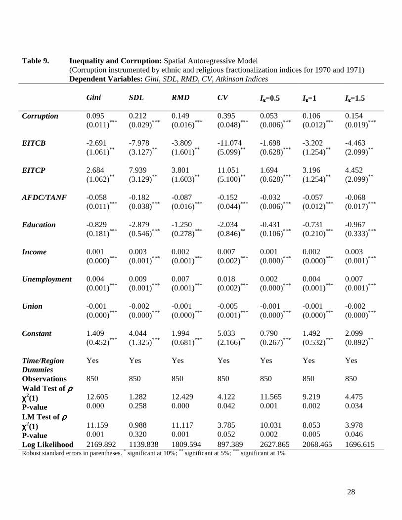
virtually the same as the ones estimated by OLS. We estimate our spatial autoregressive

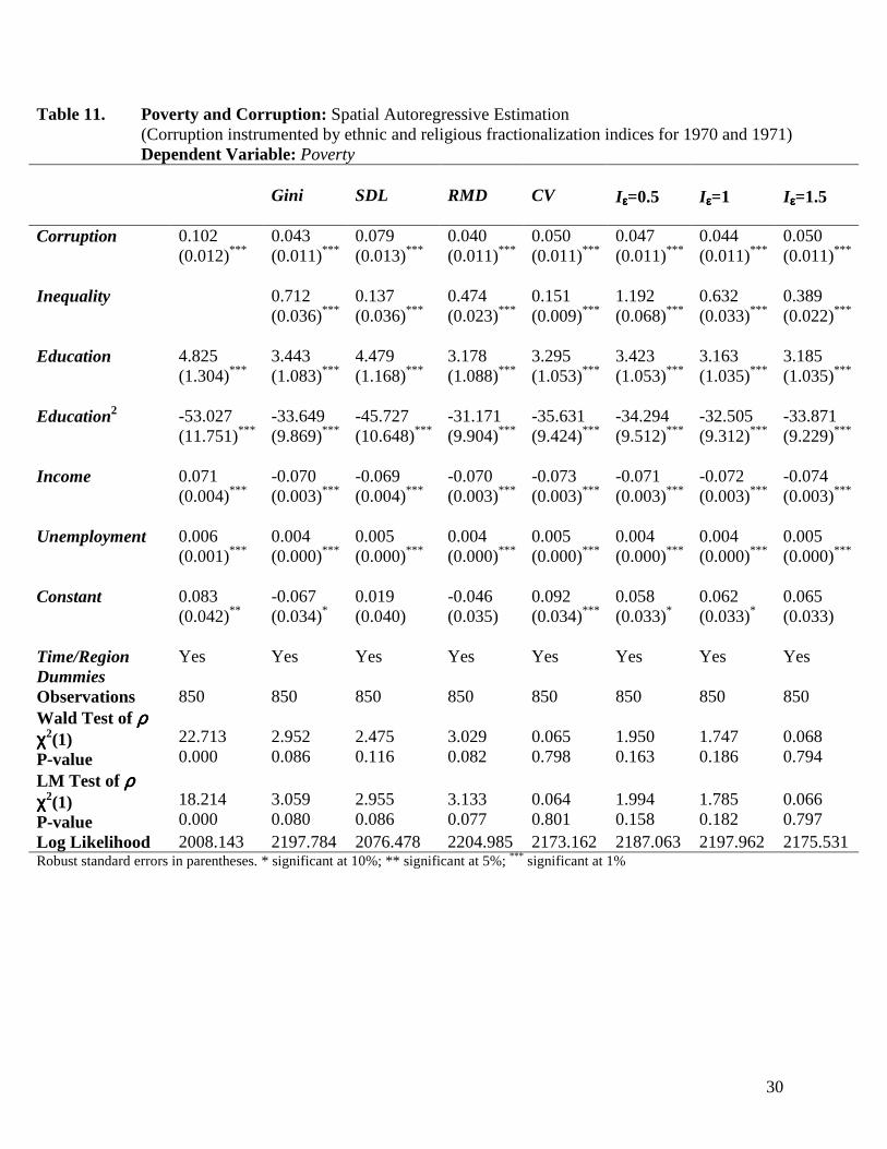
model of inequality and poverty by instrumenting Corruption with ethnic and religious

fractionalization indexes for 1970 and 1971 as well. The results are given in Tables 9 and

11. The estimated coefficients of Corruption are again positive and significant in all

regressions.

14

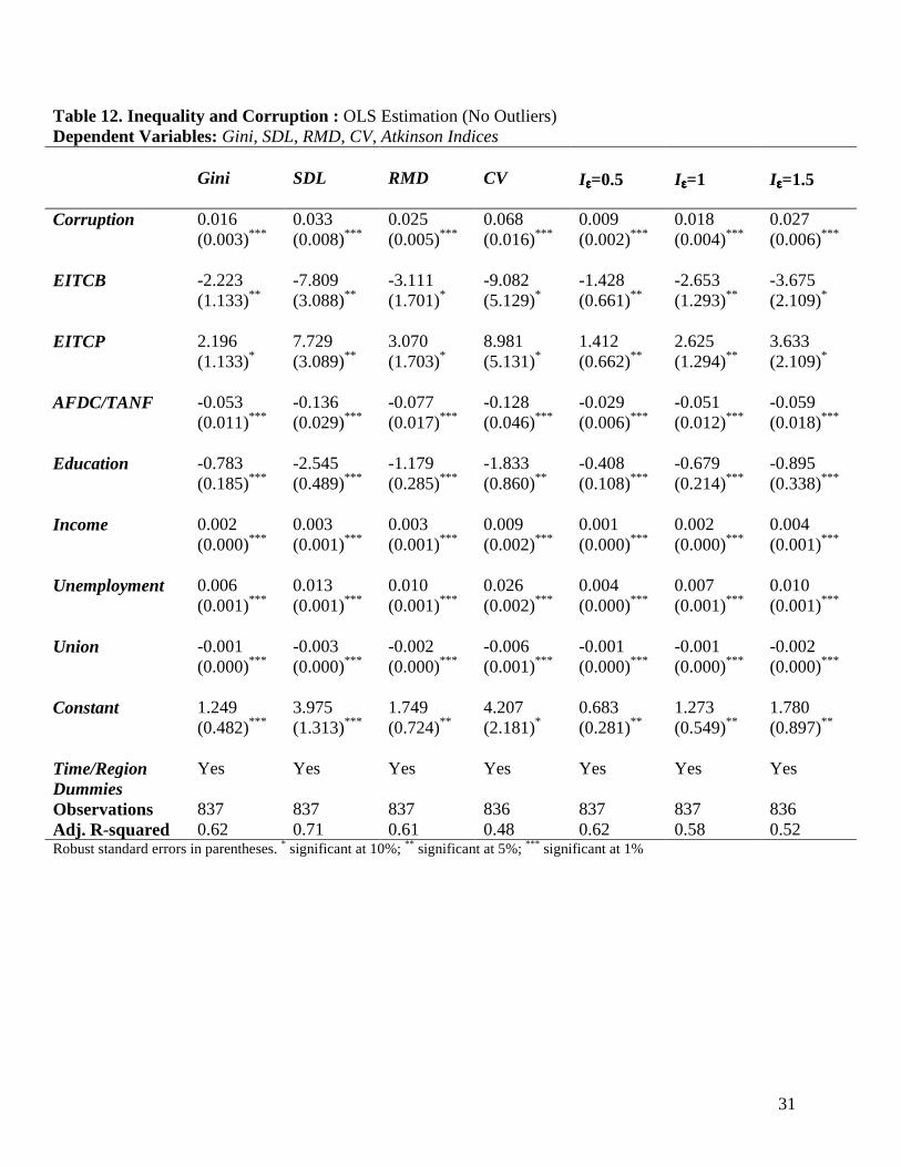
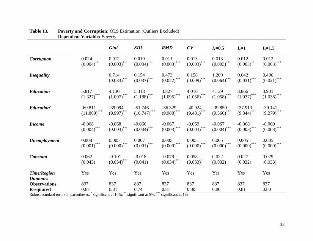
The fourth robustness issue is the presence of outliers. We estimate the

regressions without the observations identified as outliers by Hadi’s methodology. The

results are given in Tables 12 and 13. The estimated coefficient of Corruption remains

positive and significant in all estimations. It increases slightly in all estimations. One

standard deviation increase in Corruption increases Gini, for example, by 0.4 percentage

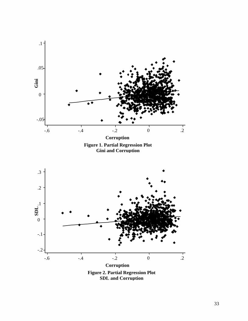
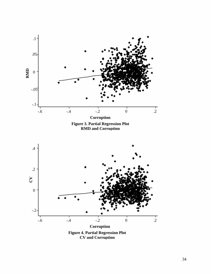
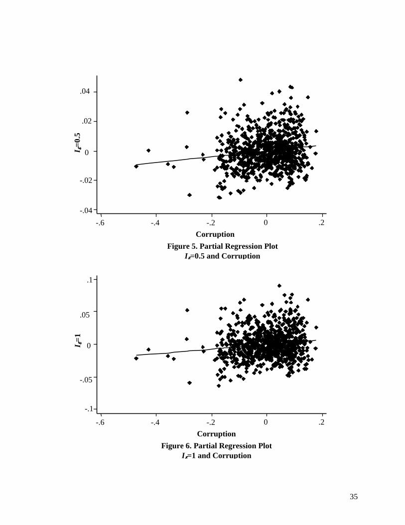
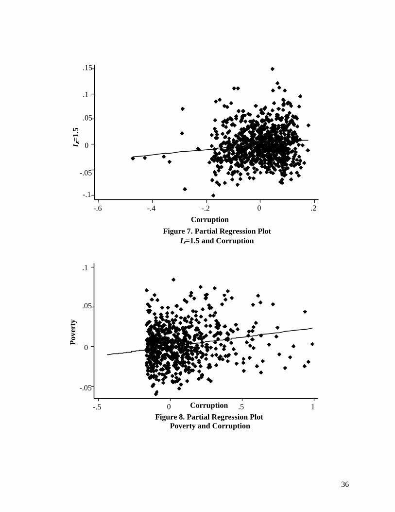
points and Poverty by 0.6 percentage points when we exclude outliers. The partial

regression plots between Corruption and our income inequality measures as well as

Corruption and Poverty are given in Figures 1 through 8.

The fifth and the last robustness issue is the stationarity of our inequality and

poverty measures. We use two commonly used unit root tests for panel data: Levin-Lin-

Chu (LLC) and Im-Pesaran-Shin (IPS). Under the null hypothesis, both tests assume that

all series in the panel are non-stationary. LLC test assumes that all series are stationary

under the alternative hypothesis whereas IPS test assumes that only a fraction of the

series in the panel is stationary. Using both tests we reject the null hypothesis of non-

stationarity of our inequality and poverty measures.

5. Conclusion

Corruption is not a phenomenon peculiar to low-income countries. It is possible to

find examples of corruption in high-income countries as well. In Germany, for example,

corruption led to an increase in cost of about 20 to 30 percent during the construction of

terminal 2 at Frankfort Airport. In Italy, the cost of major construction projects fell

significantly in the aftermath of corruption investigations in the early 1990s (Rose-

Ackerman 1999). It is not a new phenomenon either. Prior to the New Deal, welfare

15

programs in the U.S. were administered by local governments which were almost always

associated with corruption. In 1933, when unemployment reached 25 percent, the federal

government introduced welfare programs which redistributed 4 percent of the gross

national product to millions of families. Knowing that he would incur enormous losses if

the New Deal were perceived as corrupt, President Roosevelt took the fight against

corruption in the administration of welfare programs very seriously by establishing

offices to investigate complaints of corruption which led to vigorous prosecution of

corrupt government officers (Wallis, Fishback, and Kantor 2006).

In this study, we analyze the effects of corruption on income inequality and

poverty by using data from U.S. states. To our knowledge, this is in fact the first study

using data from U.S. states. Where previous analyses relied on cross-sectional variation

in cross-country data, our analysis is less sensitive to bias due to unobserved country-

specific heterogeneity. Of course, data on our variables of interest - corruption, income

inequality and poverty – as well as on control variables such as AFDC/TANF, are more

comparable across U.S. states than those across different countries. We find robust

evidence that an increase in corruption increases income inequality and poverty. One

standard deviation increase in corruption increases Gini index by 0.3 percentage points,

the standard deviation of the logarithms by 0.6 percentage points, the relative mean

deviation by 0.5 percentage points, the coefficient of variation by 1.4 percentage points,

and poverty by 0.5 percentage points.

Using Atkinson indexes with different degrees of inequality aversion helps us see

if the effects of corruption on the lower end of the distribution differ from the effects on

the higher end. We find that the coefficient estimate of corruption increases as the degree

16

of inequality aversion increases, indicating that effects of corruption on the lower end of

the distribution are higher. One standard deviation increase in corruption increases the

Atkinson indexes by 0.2, 0.4, and 0.6 percentage points for the degrees of inequality

aversion 0.5, 1, and 1.5, respectively.

17

Bibliography

Atkinson, A.B. (1970) “On the Measurement of Inequality,” Journal of Economic Theory

2: 244-263

Chetwyn, E., Chetwyn, F., and Spector, B. (2003) “Corruption and Poverty: A Review of

Recent Literature,” Mimeo, Management Systems International, Washington DC.

Chong, A. and Calderon, C. (2000a) “Institutional Quality and Income Distribution,”

Economic Development and Cultural Change 48: 761-786

Chong, A. and Calderon, C. (2000b) “Institutional Quality and Poverty Measures in a

Cross-Section of Countries,” Economics of Governance 1: 123-135.

Chong, A. and Gradstein, M. (2007) “Inequality and Institutions,” Review of Economics

and Statistics 89: 454-465.

Fisman, R. and Gatti, R. (2002) “Decentralization and Corruption: Evidence from U.S.

Federal Transfer Programs,” Public Choice 113: 25-35.

Fredriksson, P. G., List, J. A. and Millimet, D. L. (2003) “Bureaucratic Corruption,

Environmental Policy and Inbound US FDI: Theory and Evidence,” Journal of

Public Economics 87: 1407-1430

Glaeser, E. L. and Saks, R. E. (2006) “Corruption in America,” Journal of Public

Economics 90: 1053-1072.

Glaeser, E.L. (2005) “Inequality” HIER Discussion Paper 2078.

Goel, R. and Rich, D. (1989) “On the Economic Incentives for Taking Bribes,” Public

Choice 61: 269-275.

Gupta, S., Davoodi, H. and Alonso-Terme, R. (2002) “Does Corruption Affect Income

Inequality and Poverty?” Economics of Governance 3: 23-45.

18

Hirsch, B. T., Macpherson, D. A., and Vroman, W. G. (2001) “Estimates of union

Density by State,” Monthly Labor Review 124: 51-55.

Johnston, M. (1989) “Corruption, Inequality, and Change,” in P. M. Ward (Ed.),

Corruption, Development and Inequality, London: Routledge: 13-37

Keefer, P. and Knack, S. (1997) “Why Don’t Poor Countries Catch Up? A Cross-

National Test of An Institutional Explanation,” Economic Inquiry 35: 590-602.

Knack, S. (1996) “Institutions and Convergence Hypothesis: The Cross-National

Evidence,” Public Choice 87: 207-228.

Knack, S. and Keefer, P. (1995) “Institutions and Economic Performance: Cross-Country

Tests Using Alternative Institutional Measures,” Economics and Politics 7: 207-

227.

Li, H., Xu, L.C. and Zou, H. F. (2000) “Corruption, Income Distribution, and Growth,”

Economics and Politics 12: 155-182.

Mauro, P. (1995) “Corruption and Growth,” Quarterly Journal of Economics 110: 681-

812

Mo, P. H. (2001) “Corruption and Economic Growth,” Journal of Comparative

Economics 29: 66-79

Pellegrini, L. and Gerlagh, R. (2004) “Corruption’s Effect on Growth and its

Transmission Channels,” Kyklos 57:429-456.

Ravallion, M. (1997) “Can High-Inequality Developing Countries Escape Absolute

Poverty?” World Bank Policy Research Working Paper 1775.

Rose-Ackerman, S. (1999) Corruption and Government: Causes, Consequences, and

Reform, Cambridge: Cambridge University Press.

19

Sen, A. (1997) On Economic Inequality, Oxford: Oxford University Press

Tanzi, V. (1998) “Corruption Around the World: Causes, Consequences, Scope, and

Cures,” IMF Staff Papers, 45: 559-594.

Uslaner, E. (2006) “Corruption and Inequality,” UNU-WIDER Research Paper 34.

Wallis, J. J., Fishback, P. V., and Kantor, S. (2006) “Politics, Relief, and Reform:

Roosevelt’s Efforts to Control Corruption and Political Manipulation during the

New Deal,” in E. L. Glaeser and C. Goldin (Ed.), Corruption and Reform:

Lessons from America’s Economic History, Chicago: The University of Chicago

Press: 343-372.

Wu, X., Perloff, J. M., and Golan, A. (2006a) “Effects of Government Policies on

Income Distribution and Welfare,” Mimeo, Department of Agricultural and

Resource Economics, UC Berkeley.

You, J. and Khagram, S. (2005) “A Comparative Study of Inequality and Corruption,”

American Sociological Review, 70: 136-157.

20

Table 1. Worst and Best Three States

Gini

SDL

RMD

CV

Iεεεε=0.5

Iεεεε=1

Iεεεε=1.5

Poverty

Corruption

TX

TX

TX

TX

TX

TX

TX

MS

MS

MS

LA

MS

LA

LA

LA

LA

LA

TN

Wor

st 3

Sta

tes

LA

MS

LA

MS

MS

MS

MS

NM

SD

WI

VT

WI

WI

WI

WI

WI

NH

VT

VT

WI

UT

VT

VT

VT

VT

CT

OR

Bes

t 3

Stat

es

UT

UT

VT

ME

UT

UT

UT

NJ

WA

21

Table 2. Summary Statistics of Inequality Measures, Poverty Rate, and Corruption Variable

Obs

Mean

Std. Dev.

Min

Max

Gini

850

0.34

0.03

0.26

0.45

SDL

850 0.67 0.11 0.48 1.60

RMD

850 0.48 0.05 0.36 0.64

CV

850 0.55 0.12 0.28 1.01

Iεεεε=0.050

850 0.09 0.02 0.05 0.17

Iεεεε=0.100

850 0.19 0.03 0.11 0.31

Iεεεε=0.150

850 0.29 0.05 0.17 0.46

Poverty

850 0.14 0.04 0.02 0.27

Corruption 850 0.31 0.30 0 2.19

22

Table 3. Pairwise Correlations of the Inequality Measures, Poverty Rate, and Corruption

Gini

SDL

RMD

CV

Iεεεε=0.5

Iεεεε=1

Iεεεε=1.5

Poverty

Corruption

Gini

1.00

SDL

0.86 1.00

RMD

0.99 0.82 1.00

CV

0.91 0.69 0.91 1.00

Iεεεε=0.50

0.99 0.89 0.98 0.92 1.00

Iεεεε=0.100

0.98 0.82 0.98 0.97 0.99 1.00

Iεεεε=0.150

0.93 0.74 0.93 0.99 0.95 0.98 1.00

Poverty

0.56 0.31 0.60 0.59 0.54 0.58 0.58 1.00

Corruption 0.19 0.09 0.20 0.20 0.18 0.19 0.20 0.20 1.00

23

Table 4. Inequality and Corruption : OLS Estimation Dependent Variables: Gini, SDL, RMD, CV, and Atkinson Indices

Gini SDL

RMD

CV

Iεεεε=0.5

Iεεεε=1

Iεεεε=1.5

Corruption 0.011 0.019 0.017 0.047 0.006 0.013 0.019 (0.002)*** (0.006)*** (0.004)*** (0.011)*** (0.001)*** (0.003)*** (0.004)*** EITCB -2.191 -6.937 -3.059 -8.892 -1.411 -2.614 -3.604 (1.136)* (3.281)** (1.708)* (5.174)* (0.664)** (1.301)** (2.128)* EITCP 2.163 6.854 3.019 8.790 1.395 2.586 3.562 (1.137)* (3.282)** (1.710)* (5.176)* (0.665)** (1.302)** (2.128)* AFDC/TANF -0.056 -0.170 -0.083 -0.134 -0.031 -0.053 -0.061 (0.011)*** (0.038)*** (0.016)*** (0.044)*** (0.006)*** (0.012)*** (0.018)*** Education -0.807 -2.717 -1.216 -1.783 -0.418 -0.689 -0.874 (0.182)*** (0.543)*** (0.281)*** (0.848)** (0.106)*** (0.211)*** (0.333)*** Income 0.002 0.004 0.003 0.009 0.001 0.002 0.004 (0.000)*** (0.001)*** (0.000)*** (0.002)*** (0.000)*** (0.000)*** (0.001)*** Unemployment 0.006 0.013 0.010 0.027 0.004 0.007 0.011 (0.001)*** (0.001)*** (0.001)*** (0.002)*** (0.000)*** (0.001)*** (0.001)*** Union -0.001 -0.003 -0.002 -0.006 -0.001 -0.001 -0.002 (0.000)*** (0.000)*** (0.000)*** (0.001)*** (0.000)*** (0.000)*** (0.000)*** Constant 1.885 5.669 2.636 6.723 1.092 2.026 2.806 (0.814)** (2.346)** (1.223)** (3.703)* (0.476)** (0.931)** (1.522)* Time/Region Dummies

Yes Yes Yes Yes Yes Yes Yes

Observations 850 850 850 850 850 850 850 Adj. R-squared 0.61 0.64 0.59 0.46 0.60 0.56 0.50 Robust standard errors in parentheses. * significant at 10%; ** significant at 5%; *** significant at 1%

24

Table 5. Poverty and Corruption: OLS Estimation Dependent Variable: Poverty

Gini

SDL

RMD

CV

Iεεεε=0.5

AIεεεε=1

AIεεεε=1.5

Corruption 0.018 0.009 0.014 0.009 0.010 0.010 0.009 0.009 (0.003)*** (0.002)*** (0.003)*** (0.002)*** (0.002)*** (0.002)*** (0.002)*** (0.002)*** Inequality 0.718 0.156 0.476 0.158 1.216 0.644 0.406 (0.033)*** (0.037)*** (0.217)*** (0.009)*** (0.063)*** (0.031)*** (0.021)*** Education 5.548 4.028 5.121 3.724 3.772 4.005 3.699 3.661 (1.315)*** (1.091)*** (1.178)*** (1.090)*** (1.053)*** (1.054)*** (1.033)*** (1.036)*** Education2 -58.869 -38.370 -50.307 -35.597 -39.304 -38.920 -36.779 -37.509 (11.751)*** (9.959)*** (10.677)*** (9.949)*** (9.445)*** (9.528)*** (9.310)*** (9.244)*** Income -0.069 -0.068 -0.067 -0.069 -0.071 -0.068 -0.069 -0.071 (0.004)*** (0.003)*** (0.004)*** (0.003)*** (0.003)*** (0.003)*** (0.003)*** (0.003)*** Unemployment 0.008 0.005 0.007 0.005 0.005 0.005 0.005 0.005 (0.001)*** (0.000)*** (0.001)*** (0.000)*** (0.000)*** (0.000)*** (0.000)*** (0.000)*** Constant 0.075 -0.096 -0.009 -0.073 0.072 0.029 0.036 0.043 (0.042)* (0.034)*** (0.041) (0.034)** (0.033)** (0.032) (0.032) (0.033) Time/Region Dummies

Yes Yes Yes Yes Yes Yes Yes Yes

Observations 850 850 850 850 850 850 850 850 R-squared 0.67 0.81 0.74 0.82 0.80 0.80 0.80 0.79 Robust standard errors in parentheses * significant at 10%; ** significant at 5%; *** significant at 1%

25

Table 6. Inequality and Corruption: IV Estimation Dependent Variables: Gini, SDL, RMD, CV, and Atkinson Indices

Gini

SDL

RMD

CV

Iεεεε=0.5

Iεεεε=1

Iεεεε=1.5

Corruption 0.107 0.221 0.169 0.423 0.060 0.118 0.166 (0.017)*** (0.042)*** (0.027)*** (0.069)*** (0.009)*** (0.019)*** (0.027)*** EITCB -2.701 -8.003 -3.862 -10.875 -1.696 -3.170 -4.378 (1.375)** (3.377)** (2.069)* (5.496)** (0.775)** (1.488)** (2.174)** EITCP 2.693 7.963 3.854 10.854 1.692 3.165 4.368 (1.375)** (3.379)** (2.071)* (5.503)** (0.775)** (1.489)** (2.176)** AFDC/TANF -0.063 -0.185 -0.094 -0.161 -0.035 -0.061 -0.072 (0.021)*** (0.053)*** (0.033)*** (0.081)** (0.012)*** (0.023)*** (0.032)** Education -0.923 -2.958 -1.398 -2.231 -0.482 -0.815 -1.049 (0.308)*** (0.747)*** (0.482)*** (1.242)* (0.175)*** (0.339)** (0.486)** Income 0.001 0.003 0.002 0.007 0.001 0.002 0.003 (0.000)* (0.002)* (0.001)* (0.003)** (0.000)* (0.001)** (0.001)** Unemployment 0.004 0.009 0.007 0.019 0.002 0.005 0.007 (0.001)*** (0.002)*** (0.002)*** (0.004)*** (0.000)*** (0.001)*** (0.002)*** Union -0.001 -0.002 -0.002 -0.005 -0.001 -0.001 -0.002 (0.000)*** (0.001)*** (0.000)*** (0.001)*** (0.000)*** (0.000)*** (0.000)*** Constant 1.468 4.089 2.094 5.007 0.805 1.507 2.094 (0.585)** (1.435)** (0.881)** (2.341)** (0.329)** (0.633)** (0.925)** Time/Region Dummies

Yes Yes Yes Yes Yes Yes Yes

Observations 850 850 850 850 850 850 850 1st Stage F-stat. F(2,821) P-value

25.32 0.000

25.32 0.000

25.32 0.000

25.32 0.000

25.32 0.000

25.32 0.000

25.32 0.000

Hansen J-stat. χχχχ2(1) P-value

0.857 0.354

0.240 0.625

0.992 0.319

0.574 0.449

0.738 0.390

0.532 0.466

0.135 0.713

Robust standard errors in parentheses. * significant at 10%; ** significant at 5%; *** significant at 1%

26

Table 7. Poverty and Corruption : IV Estimation

Dependent Variable: Poverty

Gini SDL

RMD

CV

Iεεεε=0.5

Iεεεε=1

Iεεεε=1.5

Corruption 0.119 0.055 0.092 0.052 0.067 0.059 0.058 0.069 (0.019)*** (0.014)*** (0.018)*** (0.014)*** (0.015)*** (0.015)*** (0.015)*** (0.029)*** Inequality 0.625 0.127 0.417 0.132 1.050 0.553 0.366 (0.044)*** (0.030)*** (0.028)*** (0.012)*** (0.078)*** (0.041)*** (0.029)*** Education 2.621 2.924 2.973 2.727 2.457 2.811 2.589 2.369 (2.166) (1.343)** (1.774) (1.317)** (1.452) (1.351)** (1.329)** (1.436) Education2 -33.287 -29.659 -32.420 -27.789 -28.498 -29.369 -27.906 -27.052 (18.619)* (11.912)*** (15.377)** (11.704)*** (12.653)** (11.867)*** (11.642)*** (12.449)** Income -0.076 -0.071 -0.072 -0.071 -0.074 -0.071 -0.073 -0.075 (0.009)*** (0.004)*** (0.007)*** (0.004)*** (0.006)*** (0.005)*** (0.005)*** (0.005)*** Unemployment 0.006 0.004 0.005 0.004 0.005 0.005 0.004 0.005 (0.001)*** (0.001)*** (0.001)*** (0.001)*** (0.001)*** (0.001)*** (0.001)*** (0.001)*** Constant 0.167 -0.033 0.076 -0.016 0.123 0.079 0.085 0.099 (0.075)** (0.045) (0.063)** (0.044) (0.049)*** (0.045) (0.044) (0.049)** Time/RegionDummies Yes Yes Yes Yes Yes Yes Yes Yes Observations 850 850 850 850 850 850 850 850 1st Stage F-stat. F(2,823) P-value

25.329 0.000

17.770 0.000

22.350 0.000

17.270 0.000

19.780 0.000

18.830 0.000

18.410 0.000

19.410 0.000

Hansen J-stat. χχχχ2(1) P-value

3.524 0.061

3.373 0.067

4.224 0.039

2.754 0.097

3.989 0.046

3.641 0.056

3.878 0.049

4.947 0.026

Robust standard errors in parentheses. * significant at 10%; ** significant at 5%; *** significant at 1%

27

Table 8. Inequality and Corruption: Spatial Autoregressive Estimation

Dependent Variables: Gini, SDL, RMD, CV, Atkinson Indices

Gini SDL

RMD

CV

Iεεεε=0.5

Iεεεε=1

Iεεεε=1.5

Corruption 0.011 0.019 0.017 0.047 0.006 0.012 0.019 (0.002)*** (0.006)*** (0.003)*** (0.011)*** (0.001)*** (0.003)*** (0.004)*** EITCB -2.293 -6.989 -3.156 -9.629 -1.479 -2.789 -3.914 (1.058)** (3.155)** (1.588)** (4.978)* (0.624)** (1.232)** (2.035)* EITCP 2.269 6.912 3.122 9.535 1.466 2.765 3.874 (1.059)** (3.156)** (1.589)** (4.979)* (0.624)** (1.233)** (2.035)* AFDC/TANF -0.049 -0.165 -0.072 -0.118 -0.027 -0.047 -0.054 (0.010)*** (0.038)*** (0.016)*** (0.043)*** (0.006)*** (0.011)*** (0.017)*** Education -0.669 -2.555 -0.990 -1.435 -0.342 -0.557 -0.729 (0.185)*** (0.558)*** (0.286)*** (0.849)* (0.108)*** (0.213)*** (0.335)** Income 0.002 0.004 0.003 0.009 0.001 0.002 0.004 (0.000)*** (0.001)*** (0.001)*** (0.002)*** (0.000)*** (0.000)*** (0.001)*** Unemployment 0.006 0.012 0.009 0.025 0.003 0.007 0.010 (0.001)*** (0.001)*** (0.001)*** (0.002)*** (0.000)*** (0.001)*** (0.001)*** Union -0.001 -0.002 -0.002 -0.005 -0.001 -0.001 -0.002 (0.000)*** (0.000)*** (0.000)*** (0.001)*** (0.000)*** (0.000)*** (0.000)*** Constant 1.888 3.552 1.638 4.312 0.679 1.281 1.815 (0.449)*** (1.334)*** (0.675)** (2.115)** (0.265)*** (0.524)** (0.865)** Time/Region Dummies

Yes Yes Yes Yes Yes Yes Yes

Observations 850 850 850 850 850 850 850 Wald Test of ρρρρ χχχχ2(1) P-value

45.994 0.000

6.510 0.011

48.761 0.000

20.839 0.000

41.538 0.000

37.645 0.000

22.873 0.000

LM Test of ρρρρ χχχχ2(1) P-value

38.780 0.000

5.919 0.015

40.962 0.000

18.504 0.000

34.760 0.000

31.461 0.000

19.496 0.000

Log Likelihood 2140.739 1123.972 1778.999 872.062 2600.365 2040.098 1672.099 Robust standard errors in parentheses. * significant at 10%; ** significant at 5%; *** significant at 1%

28

Table 9. Inequality and Corruption: Spatial Autoregressive Model (Corruption instrumented by ethnic and religious fractionalization indices for 1970 and 1971)

Dependent Variables: Gini, SDL, RMD, CV, Atkinson Indices

Gini SDL

RMD

CV

Iεεεε=0.5

Iεεεε=1

Iεεεε=1.5

Corruption 0.095 0.212 0.149 0.395 0.053 0.106 0.154 (0.011)*** (0.029)*** (0.016)*** (0.048)*** (0.006)*** (0.012)*** (0.019)*** EITCB -2.691 -7.978 -3.809 -11.074 -1.698 -3.202 -4.463 (1.061)** (3.127)** (1.601)** (5.099)** (0.628)*** (1.254)** (2.099)** EITCP 2.684 7.939 3.801 11.051 1.694 3.196 4.452 (1.062)** (3.129)** (1.603)** (5.100)** (0.628)*** (1.254)** (2.099)** AFDC/TANF -0.058 -0.182 -0.087 -0.152 -0.032 -0.057 -0.068 (0.011)*** (0.038)*** (0.016)*** (0.044)*** (0.006)*** (0.012)*** (0.017)*** Education -0.829 -2.879 -1.250 -2.034 -0.431 -0.731 -0.967 (0.181)*** (0.546)*** (0.278)*** (0.846)** (0.106)*** (0.210)*** (0.333)*** Income 0.001 0.003 0.002 0.007 0.001 0.002 0.003 (0.000)*** (0.001)*** (0.001)*** (0.002)*** (0.000)*** (0.000)*** (0.001)*** Unemployment 0.004 0.009 0.007 0.018 0.002 0.004 0.007 (0.001)*** (0.001)*** (0.001)*** (0.002)*** (0.000)*** (0.001)*** (0.001)*** Union -0.001 -0.002 -0.001 -0.005 -0.001 -0.001 -0.002 (0.000)*** (0.000)*** (0.000)*** (0.001)*** (0.000)*** (0.000)*** (0.000)*** Constant 1.409 4.044 1.994 5.033 0.790 1.492 2.099 (0.452)*** (1.325)*** (0.681)*** (2.166)** (0.267)*** (0.532)*** (0.892)** Time/Region Dummies

Yes Yes Yes Yes Yes Yes Yes

Observations 850 850 850 850 850 850 850 Wald Test of ρρρρ χχχχ2(1) P-value

12.605 0.000

1.282 0.258

12.429 0.000

4.122 0.042

11.565 0.001

9.219 0.002

4.475 0.034

LM Test of ρρρρ χχχχ2(1) P-value

11.159 0.001

0.988 0.320

11.117 0.001

3.785 0.052

10.031 0.002

8.053 0.005

3.978 0.046

Log Likelihood 2169.892 1139.838 1809.594 897.389 2627.865 2068.465 1696.615 Robust standard errors in parentheses. * significant at 10%; ** significant at 5%; *** significant at 1%

29

Table 10. Poverty and Corruption: Spatial Autoregressive Estimation

Dependent Variable: Poverty

Gini SDL

RMD

CV

Iεεεε=0.5

Iεεεε=1

Iεεεε=1.5

Corruption 0.016 0.009 0.014 0.009 0.010 0.010 0.009 0.009 (0.003)*** (0.002)*** (0.003)*** (0.002)*** (0.002)*** (0.002)*** (0.002)*** (0.002)*** Inequality 0.729 0.145 0.484 0.156 1.224 0.647 0.399 (0.036)*** (0.037)*** (0.023)*** (0.009)*** (0.068)*** (0.33)*** (0.022)*** Education 6.257 3.933 5.521 3.614 3.894 3.965 3.662 3.785 (1.299)*** (1.090)*** (1.193)*** (1.092)*** (1.056)*** (1.057)*** (1.036)*** (1.038)*** Education2 -64.836 -37.469 -54.041 -34.549 -40.456 -38.537 -36.432 -38.637 (11.698)*** (9.959)*** (10.884)*** (9.967)*** (9.474)*** (9.561)*** (9.352)*** (9.279)*** Income -0.065 -0.068 -0.065 -0.068 -0.071 -0.068 -0.070 -0.071 (0.004)*** (0.003)*** (0.003)*** (0.003)*** (0.003)*** (0.003)*** (0.003)*** (0.003)*** Unemployment 0.007 0.005 0.006 0.005 0.005 0.005 0.005 0.005 (0.000)*** (0.000)*** (0.000)*** (0.000)*** (0.000)*** (0.000)*** (0.000)*** (0.000)*** Constant 0.023 -0.093 -0.029 -0.069 0.065 0.031 0.038 0.036 (0.042) (0.034)*** (0.039) (0.034)** (0.034)* (0.033) (0.032) (0.033) Time/Region Dummies

Yes Yes Yes Yes Yes Yes Yes Yes

Observations 850 850 850 850 850 850 850 850 Wald Test of ρρρρ χχχχ2(1) P-value

57.925 0.000

0.590 0.443

8.894 0.003

0.752 0.386

1.038 0.308

0.109 0.741

0.090 0.764

1.062 0.303

LM Test of ρρρρ χχχχ2(1) P-value

46.375 0.000

0.591 0.442

12.807 0.000

0.752 0.386

0.979 0.322

0.109 0.742

0.089 0.765

0.989 0.320

Log Likelihood 1991.452 2197.588 2067.939 2205.517 2170.653 2186.210 2197.126 2172.677 Robust standard errors in parentheses. * significant at 10%; ** significant at 5%; *** significant at 1%

30

Table 11. Poverty and Corruption: Spatial Autoregressive Estimation (Corruption instrumented by ethnic and religious fractionalization indices for 1970 and 1971)

Dependent Variable: Poverty

Gini SDL

RMD

CV

Iεεεε=0.5

Iεεεε=1

Iεεεε=1.5

Corruption 0.102 0.043 0.079 0.040 0.050 0.047 0.044 0.050 (0.012)*** (0.011)*** (0.013)*** (0.011)*** (0.011)*** (0.011)*** (0.011)*** (0.011)*** Inequality 0.712 0.137 0.474 0.151 1.192 0.632 0.389 (0.036)*** (0.036)*** (0.023)*** (0.009)*** (0.068)*** (0.033)*** (0.022)*** Education 4.825 3.443 4.479 3.178 3.295 3.423 3.163 3.185 (1.304)*** (1.083)*** (1.168)*** (1.088)*** (1.053)*** (1.053)*** (1.035)*** (1.035)*** Education2 -53.027 -33.649 -45.727 -31.171 -35.631 -34.294 -32.505 -33.871 (11.751)*** (9.869)*** (10.648)*** (9.904)*** (9.424)*** (9.512)*** (9.312)*** (9.229)*** Income 0.071 -0.070 -0.069 -0.070 -0.073 -0.071 -0.072 -0.074 (0.004)*** (0.003)*** (0.004)*** (0.003)*** (0.003)*** (0.003)*** (0.003)*** (0.003)*** Unemployment 0.006 0.004 0.005 0.004 0.005 0.004 0.004 0.005 (0.001)*** (0.000)*** (0.000)*** (0.000)*** (0.000)*** (0.000)*** (0.000)*** (0.000)*** Constant 0.083 -0.067 0.019 -0.046 0.092 0.058 0.062 0.065 (0.042)** (0.034)* (0.040) (0.035) (0.034)*** (0.033)* (0.033)* (0.033) Time/Region Dummies

Yes Yes Yes Yes Yes Yes Yes Yes

Observations 850 850 850 850 850 850 850 850 Wald Test of ρρρρ χχχχ2(1) P-value

22.713 0.000

2.952 0.086

2.475 0.116

3.029 0.082

0.065 0.798

1.950 0.163

1.747 0.186

0.068 0.794

LM Test of ρρρρ χχχχ2(1) P-value

18.214 0.000

3.059 0.080

2.955 0.086

3.133 0.077

0.064 0.801

1.994 0.158

1.785 0.182

0.066 0.797

Log Likelihood 2008.143 2197.784 2076.478 2204.985 2173.162 2187.063 2197.962 2175.531 Robust standard errors in parentheses. * significant at 10%; ** significant at 5%; *** significant at 1%

31

Table 12. Inequality and Corruption : OLS Estimation (No Outliers) Dependent Variables: Gini, SDL, RMD, CV, Atkinson Indices

Gini SDL

RMD

CV

Iεεεε=0.5

Iεεεε=1

Iεεεε=1.5

Corruption 0.016 0.033 0.025 0.068 0.009 0.018 0.027 (0.003)*** (0.008)*** (0.005)*** (0.016)*** (0.002)*** (0.004)*** (0.006)*** EITCB -2.223 -7.809 -3.111 -9.082 -1.428 -2.653 -3.675 (1.133)** (3.088)** (1.701)* (5.129)* (0.661)** (1.293)** (2.109)* EITCP 2.196 7.729 3.070 8.981 1.412 2.625 3.633 (1.133)* (3.089)** (1.703)* (5.131)* (0.662)** (1.294)** (2.109)* AFDC/TANF -0.053 -0.136 -0.077 -0.128 -0.029 -0.051 -0.059 (0.011)*** (0.029)*** (0.017)*** (0.046)*** (0.006)*** (0.012)*** (0.018)*** Education -0.783 -2.545 -1.179 -1.833 -0.408 -0.679 -0.895 (0.185)*** (0.489)*** (0.285)*** (0.860)** (0.108)*** (0.214)*** (0.338)*** Income 0.002 0.003 0.003 0.009 0.001 0.002 0.004 (0.000)*** (0.001)*** (0.001)*** (0.002)*** (0.000)*** (0.000)*** (0.001)*** Unemployment 0.006 0.013 0.010 0.026 0.004 0.007 0.010 (0.001)*** (0.001)*** (0.001)*** (0.002)*** (0.000)*** (0.001)*** (0.001)*** Union -0.001 -0.003 -0.002 -0.006 -0.001 -0.001 -0.002 (0.000)*** (0.000)*** (0.000)*** (0.001)*** (0.000)*** (0.000)*** (0.000)*** Constant 1.249 3.975 1.749 4.207 0.683 1.273 1.780 (0.482)*** (1.313)*** (0.724)** (2.181)* (0.281)** (0.549)** (0.897)** Time/Region Dummies

Yes Yes Yes Yes Yes Yes Yes

Observations 837 837 837 836 837 837 836 Adj. R-squared 0.62 0.71 0.61 0.48 0.62 0.58 0.52 Robust standard errors in parentheses. * significant at 10%; ** significant at 5%; *** significant at 1%

32

Table 13. Poverty and Corruption: OLS Estimation (Outliers Excluded) Dependent Variable: Poverty

Gini

SDL

RMD

CV

Iεεεε=0.5

Iεεεε=1

Iεεεε=1.5

Corruption 0.024 0.012 0.019 0.011 0.013 0.013 0.012 0.012 (0.004)*** (0.003)*** (0.004)*** (0.003)*** (0.003)*** (0.003)*** (0.003)*** (0.003)*** Inequality 0.714 0.154 0.473 0.158 1.209 0.642 0.406 (0.033)*** (0.037)*** (0.022)*** (0.009)*** (0.064)*** (0.031)*** (0.021)*** Education 5.817 4.130 5.318 3.827 4.010 4.139 3.866 3.901 (1.327)*** (1.097)*** (1.188)*** (1.096)*** (1.056)*** (1.058)*** (1.037)*** (1.038)*** Education2 -60.811 -39.094 -51.746 -36.329 -40.924 -39.850 -37.913 -39.141 (11.809)*** (9.997)*** (10.747)*** (9.988)*** (9.481)*** (9.560)*** (9.344)*** (9.279)*** Income -0.068 -0.068 -0.066 -0.067 -0.069 -0.067 -0.068 -0.069 (0.004)*** (0.003)*** (0.004)*** (0.003)*** (0.003)*** (0.004)*** (0.003)*** (0.003)*** Unemployment 0.008 0.005 0.007 0.005 0.005 0.005 0.005 0.005 (0.001)*** (0.000)*** (0.001)*** (0.000)*** (0.000)*** (0.000)*** (0.000)*** (0.000)*** Constant 0.062 -0.101 -0.018 -0.078 0.058 0.022 0.027 0.029 (0.043) (0.034)*** (0.041) (0.034)** (0.033)* (0.032) (0.032) (0.033) Time/Region Dummies

Yes Yes Yes Yes Yes Yes Yes Yes

Observations 837 837 837 837 837 837 837 837 R-squared 0.67 0.81 0.74 0.81 0.80 0.80 0.81 0.80 Robust standard errors in parentheses. * significant at 10%; ** significant at 5%; *** significant at 1%

33

-.05

0

.05

.1

Gin

i

-.6 -.4 -.2 0 .2

Corruption

Figure 1. Partial Regression Plot Gini and Corruption

-.2

-.1

0

.1

.2

.3

SDL

-.6 -.4 -.2 0 .2

Corruption

Figure 2. Partial Regression Plot SDL and Corruption

34

-.1

-.05

0

.05

.1

RM

D

-.6 -.4 -.2 0 .2

Corruption

Figure 3. Partial Regression Plot RMD and Corruption

-.2

0

.2

.4

CV

-.6 -.4 -.2 0 .2

Corruption

Figure 4. Partial Regression Plot CV and Corruption

35

-.04

-.02

0

.02

.04

I εε εε=0

.5

-.6 -.4 -.2 0 .2

Corruption

Figure 5. Partial Regression Plot Iεεεε=0.5 and Corruption

-.1

-.05

0

.05

.1

I εε εε=1

-.6 -.4 -.2 0 .2

Corruption

Figure 6. Partial Regression Plot Iεεεε=1 and Corruption

36

-.1

-.05

0

.05

.1

.15 I εε εε

=1.5

-.6 -.4 -.2 0 .2

Corruption

Figure 7. Partial Regression Plot Iεεεε=1.5 and Corruption

-.05

0

.05

.1

Pov

erty

-.5 0 .5 1 Corruption

Figure 8. Partial Regression Plot Poverty and Corruption

NOTE DI LAVORO DELLA FONDAZIONE ENI ENRICO MATTEI Fondazione Eni Enrico Mattei Working Paper Series

Our Note di Lavoro are available on the Internet at the following addresses: http://www.feem.it/Feem/Pub/Publications/WPapers/default.htm

http://www.ssrn.com/link/feem.html http://www.repec.org

http://agecon.lib.umn.edu http://www.bepress.com/feem/

NOTE DI LAVORO PUBLISHED IN 2008 CCMP 1.2008 Valentina Bosetti, Carlo Carraro and Emanuele Massetti: Banking Permits: Economic Efficiency and

Distributional Effects CCMP 2.2008 Ruslana Palatnik and Mordechai Shechter: Can Climate Change Mitigation Policy Benefit the Israeli Economy?

A Computable General Equilibrium Analysis KTHC 3.2008 Lorenzo Casaburi, Valeria Gattai and G. Alfredo Minerva: Firms’ International Status and Heterogeneity in

Performance: Evidence From Italy KTHC 4.2008 Fabio Sabatini: Does Social Capital Mitigate Precariousness? SIEV 5.2008 Wisdom Akpalu: On the Economics of Rational Self-Medication CCMP 6.2008 Carlo Carraro and Alessandra Sgobbi: Climate Change Impacts and Adaptation Strategies In Italy. An

Economic Assessment ETA 7.2008 Elodie Rouvière and Raphaël Soubeyran: Collective Reputation, Entry and Minimum Quality Standard IEM 8.2008 Cristina Cattaneo, Matteo Manera and Elisa Scarpa: Industrial Coal Demand in China: A Provincial Analysis IEM 9.2008 Massimiliano Serati, Matteo Manera and Michele Plotegher: Econometric Models for Electricity Prices: A

Critical Survey CCMP 10.2008 Bob van der Zwaan and Reyer Gerlagh: The Economics of Geological CO2 Storage and Leakage KTHC 11.2008 Maria Francesca Cracolici and Teodora Erika Uberti: Geographical Distribution of Crime in Italian Provinces:

A Spatial Econometric Analysis KTHC 12.2008 Victor Ginsburgh, Shlomo Weber and Sheila Weyers: Economics of Literary Translation. A Simple Theory and

Evidence NRM 13.2008 Carlo Giupponi, Jaroslav Mysiak and Alessandra Sgobbi: Participatory Modelling and Decision Support for

Natural Resources Management in Climate Change Research NRM 14.2008 Yaella Depietri and Carlo Giupponi: Science-Policy Communication for Improved Water Resources

Management: Contributions of the Nostrum-DSS Project CCMP 15.2008 Valentina Bosetti, Alexander Golub, Anil Markandya, Emanuele Massetti and Massimo Tavoni: Abatement Cost

Uncertainty and Policy Instrument Selection under a Stringent Climate Policy. A Dynamic Analysis KTHC 16.2008 Francesco D’Amuri, Gianmarco I.P. Ottaviano and Giovanni Peri: The Labor Market Impact of Immigration in

Western Germany in the 1990’s KTHC 17.2008 Jean Gabszewicz, Victor Ginsburgh and Shlomo Weber: Bilingualism and Communicative Benefits CCMP 18.2008 Benno Torgler, María A.GarcíaValiñas and Alison Macintyre: Differences in Preferences Towards the

Environment: The Impact of a Gender, Age and Parental Effect PRCG 19.2008 Gian Luigi Albano and Berardino Cesi: Past Performance Evaluation in Repeated Procurement: A Simple Model

of Handicapping CTN 20.2008 Pedro Pintassilgo, Michael Finus, Marko Lindroos and Gordon Munro (lxxxiv): Stability and Success of

Regional Fisheries Management Organizations CTN 21.2008 Hubert Kempf and Leopold von Thadden (lxxxiv): On Policy Interactions Among Nations: When Do

Cooperation and Commitment Matter? CTN 22.2008 Markus Kinateder (lxxxiv): Repeated Games Played in a Network CTN 23.2008 Taiji Furusawa and Hideo Konishi (lxxxiv): Contributing or Free-Riding? A Theory of Endogenous Lobby

Formation CTN 24.2008 Paolo Pin, Silvio Franz and Matteo Marsili (lxxxiv): Opportunity and Choice in Social Networks CTN 25.2008 Vasileios Zikos (lxxxiv): R&D Collaboration Networks in Mixed Oligopoly CTN 26.2008 Hans-Peter Weikard and Rob Dellink (lxxxiv): Sticks and Carrots for the Design of International Climate

Agreements with Renegotiations CTN 27.2008 Jingang Zhao (lxxxiv): The Maximal Payoff and Coalition Formation in Coalitional Games CTN 28.2008 Giacomo Pasini, Paolo Pin and Simon Weidenholzer (lxxxiv): A Network Model of Price Dispersion CTN 29.2008 Ana Mauleon, Vincent Vannetelbosch and Wouter Vergote (lxxxiv): Von Neumann-Morgenstern Farsightedly

Stable Sets in Two-Sided Matching CTN 30.2008 Rahmi İlkiliç (lxxxiv): Network of Commons CTN 31.2008 Marco J. van der Leij and I. Sebastian Buhai (lxxxiv): A Social Network Analysis of Occupational Segregation CTN 32.2008 Billand Pascal, Frachisse David and Massard Nadine (lxxxiv): The Sixth Framework Program as an Affiliation

Network: Representation and Analysis CTN 33.2008 Michèle Breton, Lucia Sbragia and Georges Zaccour (lxxxiv): Dynamic Models for International Environmental

Agreements

PRCG 34.2008 Carmine Guerriero: The Political Economy of Incentive Regulation: Theory and Evidence from US States IEM 35.2008 Irene Valsecchi: Learning from Experts PRCG 36.2008 P. A. Ferrari and S. Salini: Measuring Service Quality: The Opinion of Europeans about Utilities ETA 37.2008 Michele Moretto and Gianpaolo Rossini: Vertical Integration and Operational Flexibility CCMP 38.2008 William K. Jaeger and Van Kolpin: The Environmental Kuznets Curve from Multiple Perspectives PRCG 39.2008 Benno Torgler and Bin Dong: Corruption and Political Interest: Empirical Evidence at the Micro Level KTHC 40.2008 Laura Onofri, Paulo A.L.D. Nunes, Jasone Cenoz and Durk Gorter: Language Diversity in Urban Landscapes:

An econometric study CTN 41.2008 Michel Le Breton, Valery Makarov, Alexei Savvateev and Shlomo Weber (lxxxiv): Multiple Membership and

Federal Sructures NRM 42.2008 Gideon Kruseman and Lorenzo Pellegrini: Institutions and Forest Management: A Case Study from Swat,

Pakistan SIEV 43.2008 Pietro Caratti and Ludovico Ferraguto: Analysing Regional Sustainability Through a Systemic Approach: The

Lombardy Case Study KTHC 44.2008 Barbara Del Corpo, Ugo Gasparino, Elena Bellini and William Malizia: Effects of Tourism Upon the Economy

of Small and Medium-Sized European Cities. Cultural Tourists and “The Others” CTN 45.2008 Dinko Dimitrov and Emiliya Lazarova: Coalitional Matchings ETA 46.2008 Joan Canton, Maia David and Bernard Sinclair-Desgagné: Environmental Regulation and Horizontal Mergers

in the Eco-industry ETA 47.2008 Stéphane Hallegatte: A Proposal for a New Prescriptive Discounting Scheme: The Intergenerational Discount

Rate KTHC 48.2008 Angelo Antoci, Paolo Russu and Elisa Ticci: Structural Change, Environment and Well-being: Interactions

Between Production and Consumption Choices of the Rich and the Poor in Developing Countries PRCG 49.2008 Gian Luigi Albano, Federico Dini Roberto Zampino and Marta Fana: The Determinants of Suppliers’

Performance in E-Procurement: Evidence from the Italian Government’s E-Procurement Platform CCMP 50.2008 Inmaculada Martínez-Zarzoso: The Impact of Urbanization on CO2 Emissions: Evidence from Developing

Countries KTHC 51.2008 Michele Moretto and Sergio Vergalli: Managing Migration through Quotas: an Option-theory Perspective KTHC 52.2008 Ugo Gasparino, Elena Bellini, Barbara Del Corpo and William Malizia: Measuring the Impact of Tourism

Upon Urban Economies: A Review of Literature ETA 53.2008 Reyer Gerlagh, Snorre Kverndokk and Knut Einar Rosendahl: Linking Environmental and Innovation Policy KTHC 54.2008 Oguzhan C. Dincer and Burak Gunalp: Corruption, Income Inequality, and Poverty in the United States

(lxxxiv) This paper was presented at the 13th Coalition Theory Network Workshop organised by the Fondazione Eni Enrico Mattei (FEEM), held in Venice, Italy on 24-25 January 2008.

2008 SERIES

CCMP Climate Change Modelling and Policy (Editor: Carlo Carraro)

SIEV Sustainability Indicators and Environmental Valuation (Editor: Anil Markandya)

NRM Natural Resources Management (Editor: Carlo Giupponi)

KTHC Knowledge, Technology, Human Capital (Editor: Gianmarco Ottaviano)

IEM International Energy Markets (Editor: Matteo Manera)

CSRM Corporate Social Responsibility and Sustainable Management (Editor: Giulio Sapelli)

PRCG Privatisation Regulation Corporate Governance (Editor: Bernardo Bortolotti)

ETA Economic Theory and Applications (Editor: Carlo Carraro)

CTN Coalition Theory Network