COSC 522 – Machine Learning

Lecture 11 – Perceptron

Hairong Qi, Gonzalez Family ProfessorElectrical Engineering and Computer ScienceUniversity of Tennessee, Knoxvillehttp://www.eecs.utk.edu/faculty/qiEmail: hqi@utk.edu

Course Website: http://web.eecs.utk.edu/~hqi/cosc522/

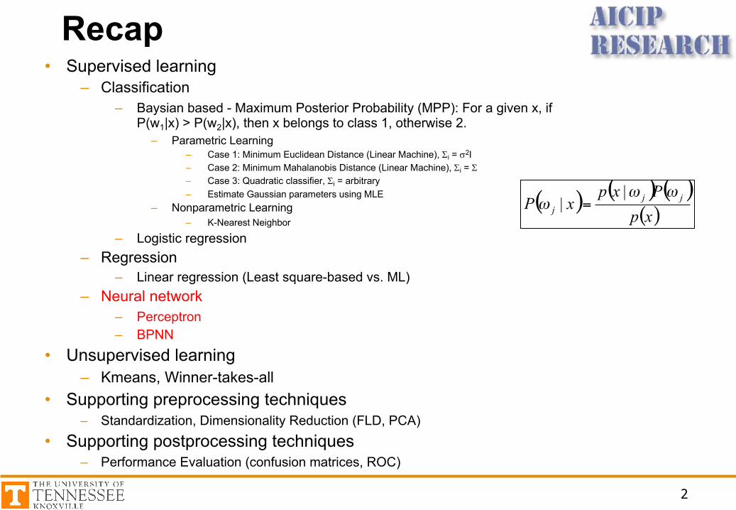
Recap• Supervised learning

– Classification– Baysian based - Maximum Posterior Probability (MPP): For a given x, if

P(w1|x) > P(w2|x), then x belongs to class 1, otherwise 2.– Parametric Learning

– Case 1: Minimum Euclidean Distance (Linear Machine), Si = s2I– Case 2: Minimum Mahalanobis Distance (Linear Machine), Si = S– Case 3: Quadratic classifier, Si = arbitrary– Estimate Gaussian parameters using MLE

– Nonparametric Learning– K-Nearest Neighbor

– Logistic regression– Regression

– Linear regression (Least square-based vs. ML)– Neural network

– Perceptron– BPNN

• Unsupervised learning– Kmeans, Winner-takes-all

• Supporting preprocessing techniques– Standardization, Dimensionality Reduction (FLD, PCA)

• Supporting postprocessing techniques– Performance Evaluation (confusion matrices, ROC)

2

( ) ( ) ( )( )xpPxp

xP jjj

ωωω

|| =

Questions• The anatomy of biological neuron• What is action potential and how does it work?• The analogy between biological neuron and perceptron• What is the cost function of perceptron?• How is perceptron trained?• What is the limitation of perceptron?• Again, what is an epoch?

3

A wrong direction – the first AI winter• One argument: Instead of understanding the

human brain, we understand the computer. Therefore, NN dies out in 70s.

• 1980s, Japan started “the fifth generation computer research project”, namely, “knowledge information processing computer system”. The project aims to improve logical reasoning to reach the speed of numerical calculation. This project proved an abortion, but it brought another climax to AI research and NN research.

4

5

Biological neuron

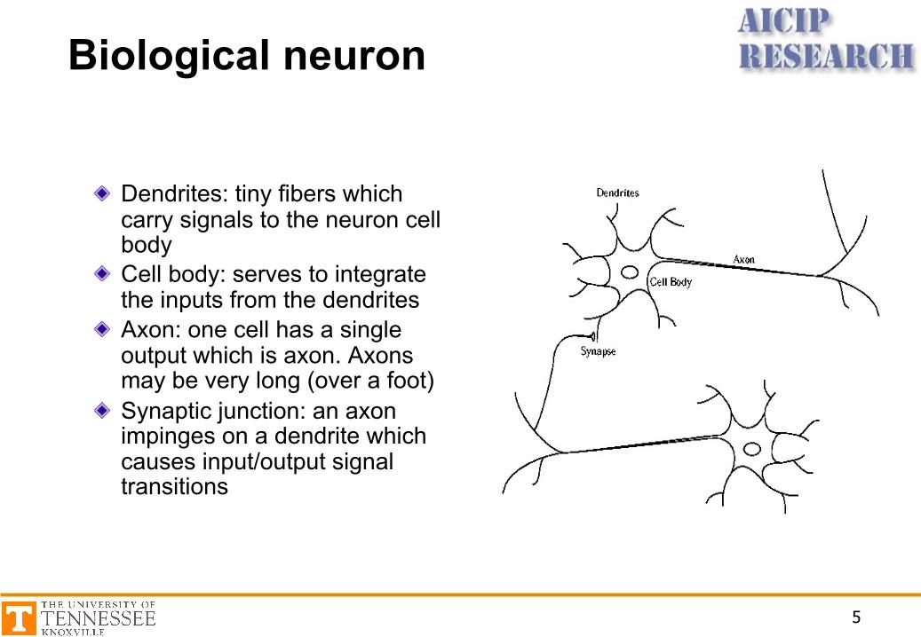
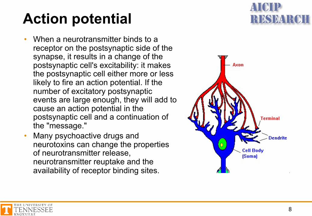
Dendrites: tiny fibers which carry signals to the neuron cell bodyCell body: serves to integrate the inputs from the dendritesAxon: one cell has a single output which is axon. Axons may be very long (over a foot)Synaptic junction: an axon impinges on a dendrite which causes input/output signal transitions

6

Synapse

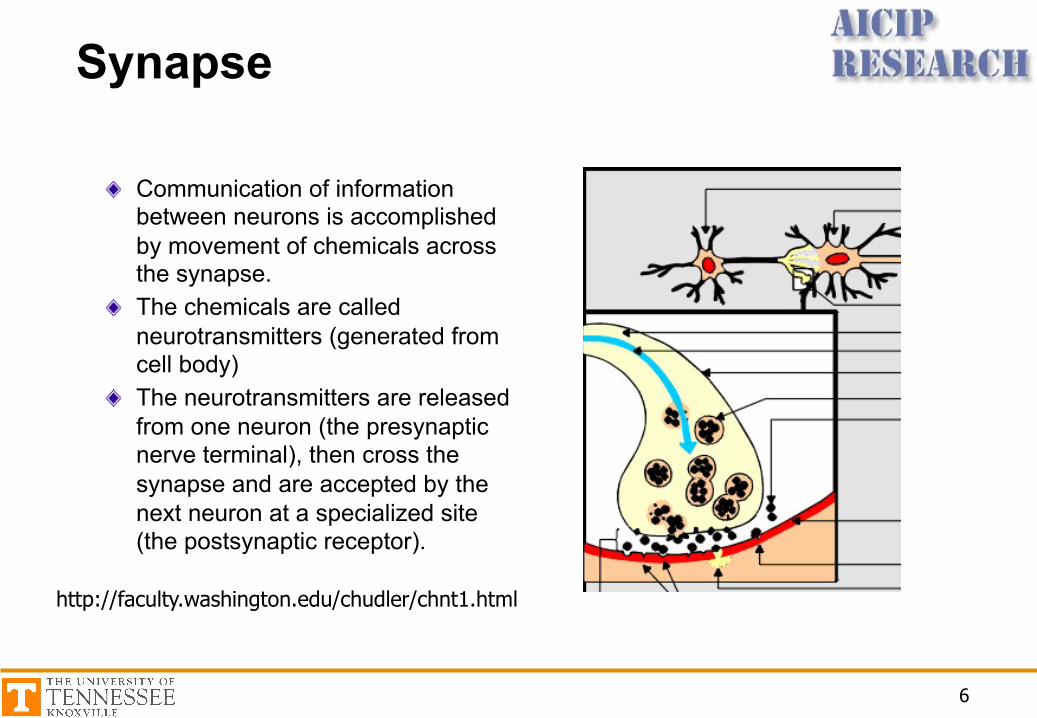
Communication of information between neurons is accomplished by movement of chemicals across the synapse.The chemicals are called neurotransmitters (generated from cell body)The neurotransmitters are released from one neuron (the presynaptic nerve terminal), then cross the synapse and are accepted by the next neuron at a specialized site (the postsynaptic receptor).

http://faculty.washington.edu/chudler/chnt1.html

7

The discovery of neurotransmitters

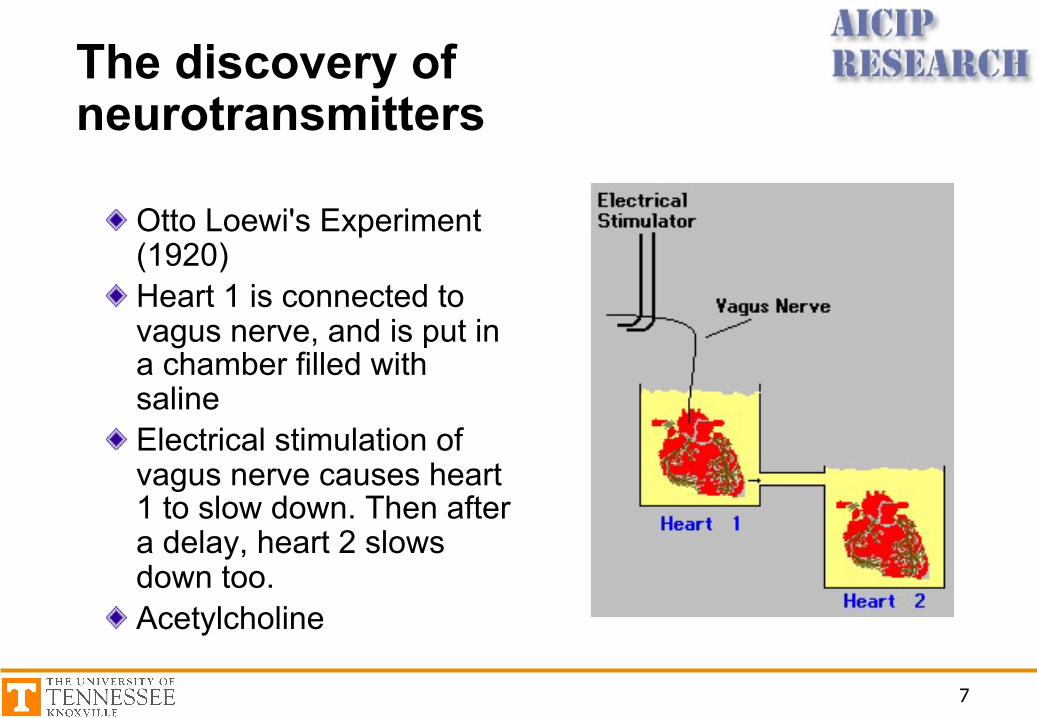
Otto Loewi's Experiment (1920)Heart 1 is connected to vagus nerve, and is put in a chamber filled with salineElectrical stimulation of vagus nerve causes heart 1 to slow down. Then after a delay, heart 2 slows down too.Acetylcholine

8

Action potential• When a neurotransmitter binds to a

receptor on the postsynaptic side of the synapse, it results in a change of the postsynaptic cell's excitability: it makes the postsynaptic cell either more or less likely to fire an action potential. If the number of excitatory postsynaptic events are large enough, they will add to cause an action potential in the postsynaptic cell and a continuation of the "message."

• Many psychoactive drugs and neurotoxins can change the properties of neurotransmitter release, neurotransmitter reuptake and the availability of receptor binding sites.

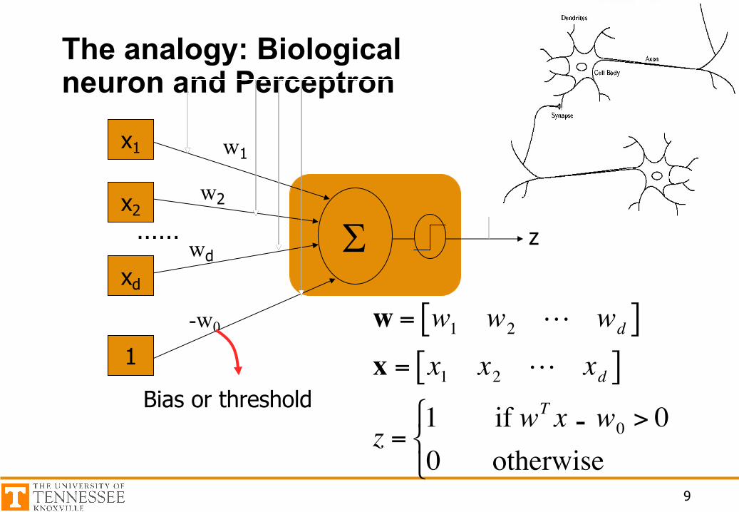
The analogy: Biological neuron and Perceptron

9

S

w1

w2

wd

x1

x2

xd

1

z

€

w = w1 w2 wd[ ]x = x1 x2 xd[ ]

z =1 if wT x + w0 > 00 otherwise

" # $

-w0

Bias or threshold

……

-

Questions• The anatomy of biological neuron• What is action potential and how does it work?• The analogy between biological neuron and perceptron• What is the cost function of perceptron?• How is perceptron trained?• What is the limitation of perceptron?• Again, what is an epoch?

10

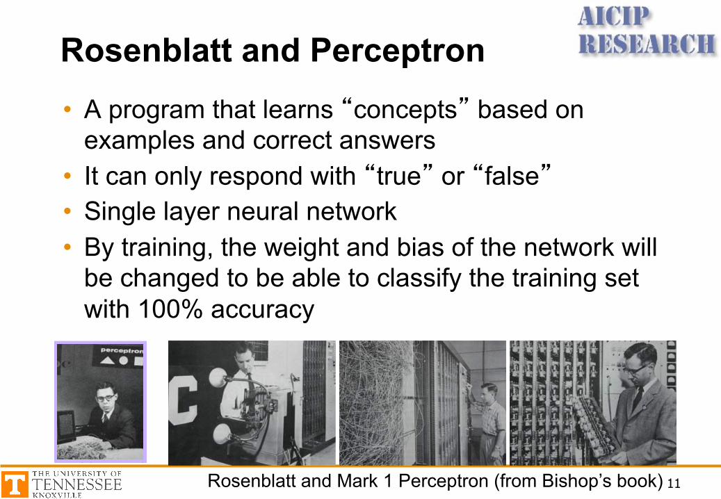
Rosenblatt and Perceptron• A program that learns “concepts” based on

examples and correct answers• It can only respond with “true” or “false”• Single layer neural network• By training, the weight and bias of the network will

be changed to be able to classify the training set with 100% accuracy

11

4.1. Discriminant Functions 193

where the nonlinear activation function f(·) is given by a step function of the form

f(a) ={

+1, a ! 0−1, a < 0. (4.53)

The vector φ(x) will typically include a bias component φ0(x) = 1. In earlierdiscussions of two-class classification problems, we have focussed on a target codingscheme in which t ∈ {0, 1}, which is appropriate in the context of probabilisticmodels. For the perceptron, however, it is more convenient to use target valuest = +1 for class C1 and t = −1 for class C2, which matches the choice of activationfunction.

The algorithm used to determine the parameters w of the perceptron can mosteasily be motivated by error function minimization. A natural choice of error func-tion would be the total number of misclassified patterns. However, this does not leadto a simple learning algorithm because the error is a piecewise constant functionof w, with discontinuities wherever a change in w causes the decision boundary tomove across one of the data points. Methods based on changing w using the gradi-ent of the error function cannot then be applied, because the gradient is zero almosteverywhere.

We therefore consider an alternative error function known as the perceptron cri-terion. To derive this, we note that we are seeking a weight vector w such thatpatterns xn in class C1 will have wTφ(xn) > 0, whereas patterns xn in class C2

have wTφ(xn) < 0. Using the t ∈ {−1, +1} target coding scheme it follows thatwe would like all patterns to satisfy wTφ(xn)tn > 0. The perceptron criterionassociates zero error with any pattern that is correctly classified, whereas for a mis-classified pattern xn it tries to minimize the quantity −wTφ(xn)tn. The perceptroncriterion is therefore given by

EP(w) = −∑

n∈M

wTφntn (4.54)

Frank Rosenblatt1928–1969

Rosenblatt’s perceptron played animportant role in the history of ma-chine learning. Initially, Rosenblattsimulated the perceptron on an IBM704 computer at Cornell in 1957,but by the early 1960s he had built

special-purpose hardware that provided a direct, par-allel implementation of perceptron learning. Many ofhis ideas were encapsulated in “Principles of Neuro-dynamics: Perceptrons and the Theory of Brain Mech-anisms” published in 1962. Rosenblatt’s work wascriticized by Marvin Minksy, whose objections werepublished in the book “Perceptrons”, co-authored with

Seymour Papert. This book was widely misinter-preted at the time as showing that neural networkswere fatally flawed and could only learn solutions forlinearly separable problems. In fact, it only provedsuch limitations in the case of single-layer networkssuch as the perceptron and merely conjectured (in-correctly) that they applied to more general networkmodels. Unfortunately, however, this book contributedto the substantial decline in research funding for neu-ral computing, a situation that was not reversed un-til the mid-1980s. Today, there are many hundreds,if not thousands, of applications of neural networksin widespread use, with examples in areas such ashandwriting recognition and information retrieval be-ing used routinely by millions of people.

196 4. LINEAR MODELS FOR CLASSIFICATION

Figure 4.8 Illustration of the Mark 1 perceptron hardware. The photograph on the left shows how the inputswere obtained using a simple camera system in which an input scene, in this case a printed character, wasilluminated by powerful lights, and an image focussed onto a 20 × 20 array of cadmium sulphide photocells,giving a primitive 400 pixel image. The perceptron also had a patch board, shown in the middle photograph,which allowed different configurations of input features to be tried. Often these were wired up at random todemonstrate the ability of the perceptron to learn without the need for precise wiring, in contrast to a moderndigital computer. The photograph on the right shows one of the racks of adaptive weights. Each weight wasimplemented using a rotary variable resistor, also called a potentiometer, driven by an electric motor therebyallowing the value of the weight to be adjusted automatically by the learning algorithm.

Aside from difficulties with the learning algorithm, the perceptron does not pro-vide probabilistic outputs, nor does it generalize readily to K > 2 classes. The mostimportant limitation, however, arises from the fact that (in common with all of themodels discussed in this chapter and the previous one) it is based on linear com-binations of fixed basis functions. More detailed discussions of the limitations ofperceptrons can be found in Minsky and Papert (1969) and Bishop (1995a).

Analogue hardware implementations of the perceptron were built by Rosenblatt,based on motor-driven variable resistors to implement the adaptive parameters wj .These are illustrated in Figure 4.8. The inputs were obtained from a simple camerasystem based on an array of photo-sensors, while the basis functions φ could bechosen in a variety of ways, for example based on simple fixed functions of randomlychosen subsets of pixels from the input image. Typical applications involved learningto discriminate simple shapes or characters.

At the same time that the perceptron was being developed, a closely relatedsystem called the adaline, which is short for ‘adaptive linear element’, was beingexplored by Widrow and co-workers. The functional form of the model was the sameas for the perceptron, but a different approach to training was adopted (Widrow andHoff, 1960; Widrow and Lehr, 1990).

4.2. Probabilistic Generative Models

We turn next to a probabilistic view of classification and show how models withlinear decision boundaries arise from simple assumptions about the distribution ofthe data. In Section 1.5.4, we discussed the distinction between the discriminativeand the generative approaches to classification. Here we shall adopt a generative

Rosenblatt and Mark 1 Perceptron (from Bishop’s book)

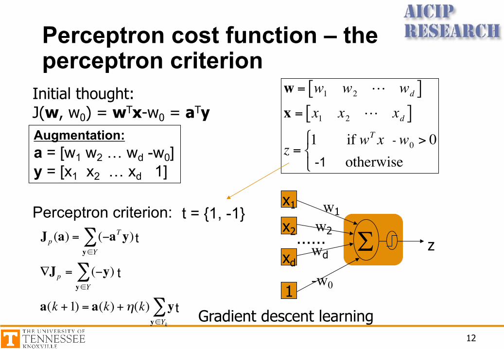
Perceptron cost function – the perceptron criterion

12

Initial thought:J(w, w0) = wTx-w0 = aTy

Gradient descent learning

Augmentation:a = [w1 w2 … wd -w0]y = [x1 x2 … xd 1]

€

w = w1 w2 wd[ ]x = x1 x2 xd[ ]

z =1 if wT x + w0 > 00 otherwise

" # $

-

Perceptron criterion:

€

Jp (a) = (−aTy)y∈Y∑

∇Jp = (−y)y∈Y∑

a(k +1) = a(k) +η(k) yy∈Yk

∑

t

t

t

Sw1w2wd

x1x2xd

1

z

-w0

……t = {1, -1}

-1

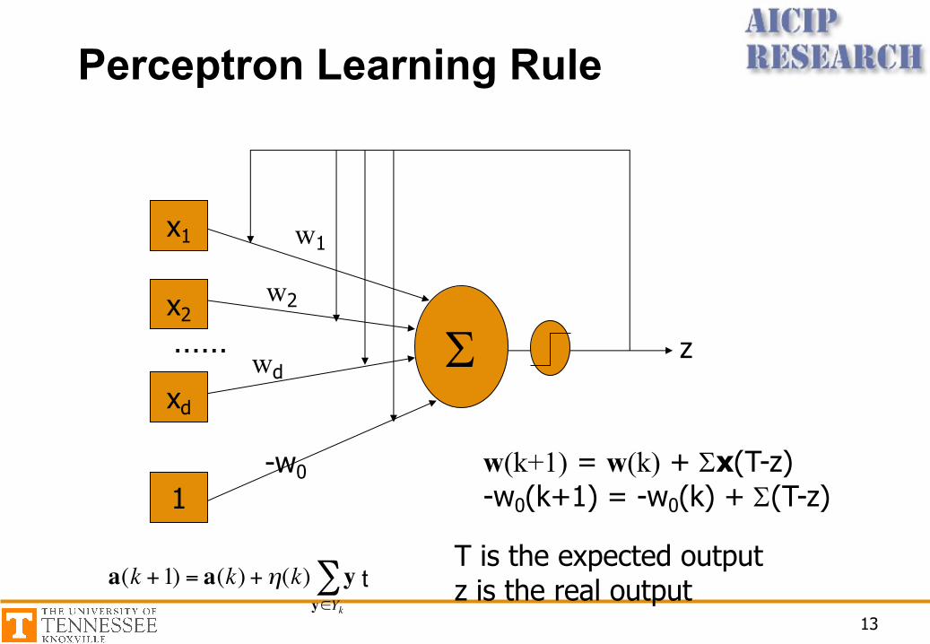
Perceptron Learning Rule

13

S

w1

w2

wd

x1

x2

xd

1

z

-w0

……

€

a(k +1) = a(k) +η(k) yy∈Yk

∑ t

w(k+1) = w(k) + Sx(T-z)-w0(k+1) = -w0(k) + S(T-z)

T is the expected outputz is the real output

Training

• Step1: Samples are presented to the network• Step2: If the output is correct, no change is made;

Otherwise, the weight and biases will be updated based on perceptron learning rule. That is,

– For Class 1, add x onto the current estimate w– For Class -1, subtract x from w

• Step3: An entire pass through all the training set is called an “epoch”. If no change has been made for the epoch, stop. Otherwise, go back Step1

14

Exercise (AND Logic)

15

w1w2

x1

x2

1

z

-w0

x1 x2 T0 0 01 0 00 1 01 1 1

w1 w2 -w0

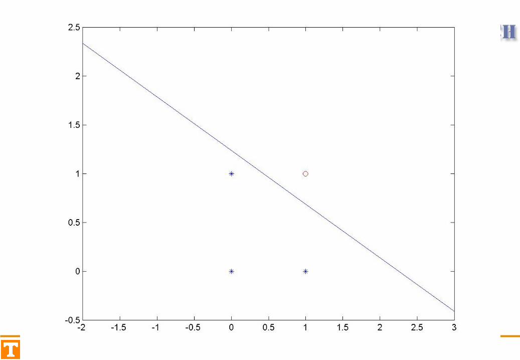
Visualizing the Decision Rule

16

Limitations

• The output only has two values (1 or 0)• Can only classify samples which are linearly

separable (straight line or straight plane)• Can’t train network functions like XOR

17

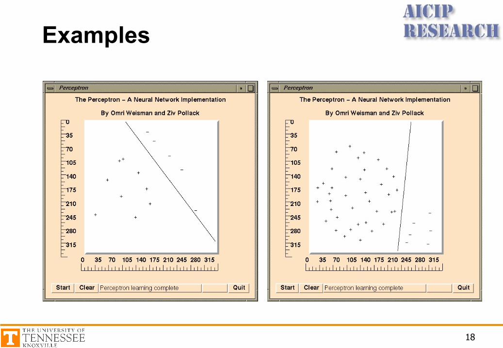
Examples

18

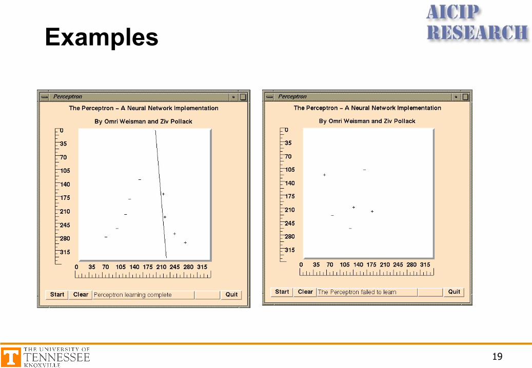
Examples

19