Embed Size (px)
Citation preview

Algorithms Analysis
lecture 8
Minimum and Maximum Alg+
Dynamic Programming

Min and Max
• The minimum of a set of elements:
– The first order statistic i = 1
• The maximum of a set of elements:
– The n-th order statistic i = n
• The median is the “halfway point” of the set
– i = (n+1)/2, is unique when n is odd
– i = (n+1)/2 = n/2 (lower median) and (n+1)/2 =
n/2+1 (upper median), when n is even

Finding Minimum or Maximum
Alg.: MINIMUM(A, n)min A[1]←for i 2← to n do if min > A[i]
then min A[i]←return min
• How many comparisons are needed?– n – 1: each element, except the minimum, must be compared to
a smaller element at least once
– The same number of comparisons are needed to find the maximum
– The algorithm is optimal with respect to the number of comparisons performed

Simultaneous Min, Max
• Find min and max independently
– Use n – 1 comparisons for each ⇒ total of 2n – 2
• At most 3n/2 comparisons are needed
– Process elements in pairs
– Maintain the minimum and maximum of elements seen so far
– Don’t compare each element to the minimum and maximum
separately
– Compare the elements of a pair to each other
– Compare the larger element to the maximum so far, and
compare the smaller element to the minimum so far
– This leads to only 3 comparisons for every 2 elements

Analysis of Simultaneous Min, Max
• Setting up initial values:
– n is odd:
– n is even:
• Total number of comparisons:
– n is odd: we do 3(n-1)/2 comparisons
– n is even: we do 1 initial comparison + 3(n-2)/2 more
comparisons = 3n/2 - 2 comparisons
set both min and max to the first element
compare the first two elements, assign the smallest one to min and the largest one to max

Example: Simultaneous Min, Max
• n = 5 (odd), array A = {2, 7, 1, 3, 4}
– Set min = max = 2
– Compare elements in pairs:
– 1 < 7 ⇒ compare 1 with min and 7 with max
⇒ min = 1, max = 7
– 3 < 4 ⇒ compare 3 with min and 4 with max
⇒ min = 1, max = 7
We performed: 3(n-1)/2 = 6 comparisons
3 comparisons
3 comparisons

Example: Simultaneous Min, Max
• n = 6 (even), array A = {2, 5, 3, 7, 1, 4}
– Compare 2 with 5: 2 < 5
– Set min = 2, max = 5
– Compare elements in pairs:
– 3 < 7 ⇒ compare 3 with min and 7 with max
⇒ min = 2, max = 7
– 1 < 4 ⇒ compare 1 with min and 4 with max
⇒ min = 1, max = 7
We performed: 3n/2 - 2 = 7 comparisons
3 comparisons
3 comparisons
1 comparison

Advanced Design and AnalysisTechniques
T Covers important techniques for the design and analysis of efficient algorithms: such as dynamic programming, greedy algorithms.

Dynamic Programming
• Well known algorithm design techniques:.– Divide-and-conquer algorithms
• Another strategy for designing algorithms is dynamic programming.– Used when problem breaks down into recurring small
subproblems
• Dynamic programming is typically applied to optimization problems. In such problem there can be many solutions. Each solution has a value, and we wish to find a solution with the optimal value.

Divide-and-conquer
• Divide-and-conquer method for algorithm design:
• Divide: If the input size is too large to deal with in a straightforward manner, divide the problem into two or more disjoint subproblems
• Conquer: conquer recursively to solve the subproblems
• Combine: Take the solutions to the subproblems and “merge” these solutions into a solution for the original problem

Divide-and-conquer - Example

Dynamic programming
• Dynamic programming is a way of improving on inefficient divide-and-conquer algorithms.
• By “inefficient”, we mean that the same recursive call is made over and over.
• If same subproblem is solved several times, we can use table to store result of a subproblem the first time it is computed and thus never have to recompute it again.
• Dynamic programming is applicable when the subproblems are dependent, that is, when subproblems share subsubproblems.
• “Programming” refers to a tabular method

Difference between DP and Divide-and-Conquer
• Using Divide-and-Conquer to solve these problems is inefficient because the same common subproblems have to be solved many times.
• DP will solve each of them once and their answers are stored in a table for future use.

Elements of Dynamic Programming (DP)
DP is used to solve problems with the following characteristics:
• Simple subproblems – We should be able to break the original problem to smaller
subproblems that have the same structure
• Optimal substructure of the problems – The optimal solution to the problem contains within optimal
solutions to its subproblems.
• Overlapping sub-problems – there exist some places where we solve the same subproblem more
than once.

Steps to Designing a Dynamic Programming Algorithm
• Characterize optimal substructure
2. Recursively define the value of an optimal solution
3. Compute the value bottom up
4. (if needed) Construct an optimal solution

Fibonacci Numbers
• Fn= Fn-1+ Fn-2 n ≥ 2• F0 =0, F1 =1• 0, 1, 1, 2, 3, 5, 8, 13, 21, 34, 55, …
• Straightforward recursive procedure is slow!
• Let’s draw the recursion tree

Fibonacci Numbers
Fibonacci Numbers
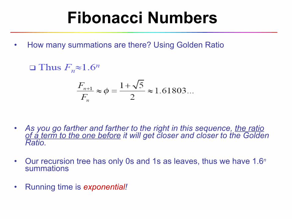
• How many summations are there? Using Golden Ratio
• As you go farther and farther to the right in this sequence, the ratio of a term to the one before it will get closer and closer to the Golden Ratio.
• Our recursion tree has only 0s and 1s as leaves, thus we have 1.6n summations
• Running time is exponential!

Fibonacci Numbers
• We can calculate Fn in linear time by remembering solutions to the solved subproblems – dynamic programming
• Compute solution in a bottom-up fashion
• In this case, only two values need to be remembered at any time

Ex1:Assembly-line scheduling
E Automobiles factory with two assembly lines.
A Each line has the same number “n” of stations. Numbered j = 1, 2, ..., n.
2 We denote the jth station on line i (where i is 1 or 2) by Si,j .
W The jth station on line 1 (S1,j) performs the same function as the jth station on line 2 (S2,j ).
s The time required at each station varies, even between stations at the same position on the two different lines, as each assembly line has different technology.
h time required at station Si,j is (ai,j) .
t There is also an entry time (ei) for the chassis(هيكل to enter (assembly line i and an exit time (xi) for the completed auto to exit assembly line i.

Ex1:Assembly-line scheduling
•(Time between adjacent stations are nearly 0).

Problem Definition
• Problem: Given all these costs, what stations should be chosen from line 1 and from line 2 for minimizing the total time for car assembly.
• “Brute force” is to try all possibilities.– requires to examine Omega(2n) possibilities– Trying all 2n subsets is infeasible when n is large.
– Simple example : 2 station (2n) possibilities =4
start end

Step 1: Optimal Solution Structure
S optimal substructure : choosing the best path to Sij.
• The structure of the fastest way through the factory (from the starting point)
• The fastest possible way to get through Si,1 (i = 1, 2) – Only one way: from entry starting point to Si,1– take time is entry time (ei)

Step 1: Optimal Solution Structure
• The fastest possible way to get through Si,j (i = 1, 2) (j = 2, 3, ..., n). Two choices:
– Stay in the same line: Si,j-1 Si,j– Time is Ti,j-1 + ai,j
• If the fastest way through Si,j is through Si,j-1, it must have taken a fastest way through Si,j-1
– Transfer to other line: S3-i,j-1 Si,j– Time is T3-i,j-1 + t3-i,j-1 + ai,j
• Same as above

Step 1: Optimal Solution Structure
• An optimal solution to a problem– finding the fastest way to get through Si,j
• contains within it an optimal solution to sub-problems– finding the fastest way to get through either Si,j-1 or S3-i,j-1
• Fastest way from starting point to Si,j is either:– The fastest way from starting point to Si,j-1 and then directly
from Si,j-1 to Si,jor– The fastest way from starting point to S3-i,j-1 then a transfer
from line 3-i to line i and finally to Si,j
Optimal Substructure.

Example


Step 2: Recursive Solution
• Define the value of an optimal solution recursively in terms of the optimal solution to sub-problems
• Sub-problem here – finding the fastest way through station j on both lines (i=1,2)– Let fi [j] be the fastest possible time to go from starting point
through Si,j
• The fastest time to go all the way through the factory: f*
• x1 and x2 are the exit times from lines 1 and 2, respectively
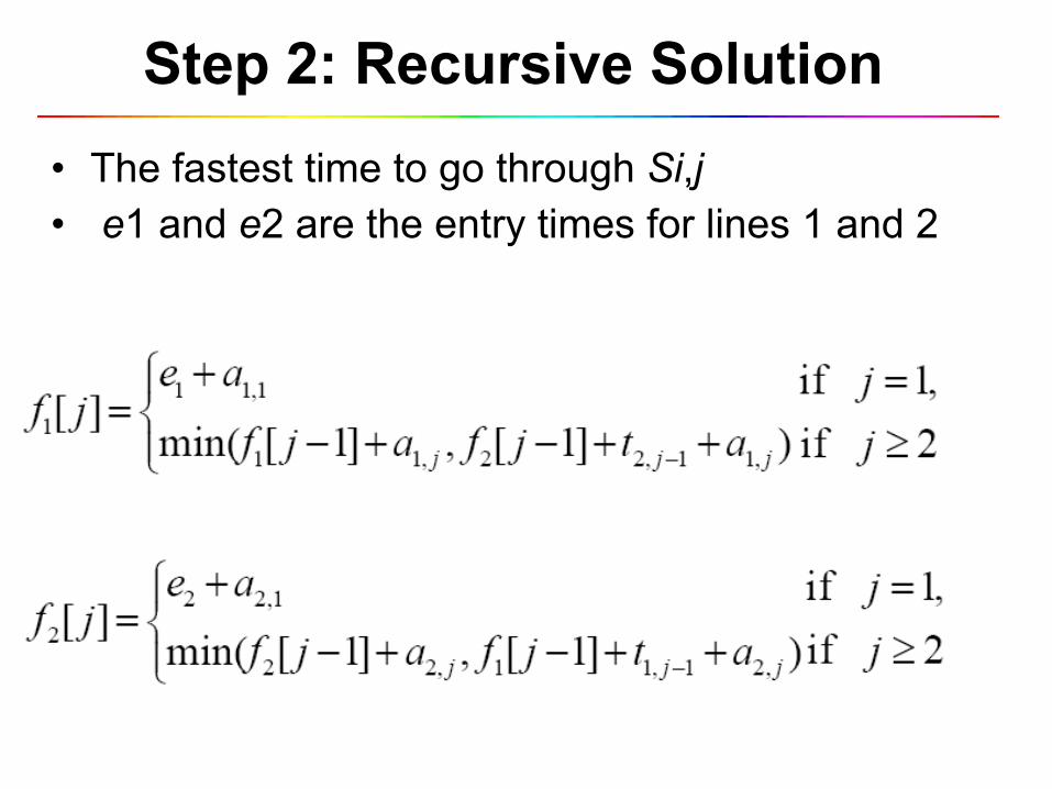
Step 2: Recursive Solution
• The fastest time to go through Si,j• e1 and e2 are the entry times for lines 1 and 2
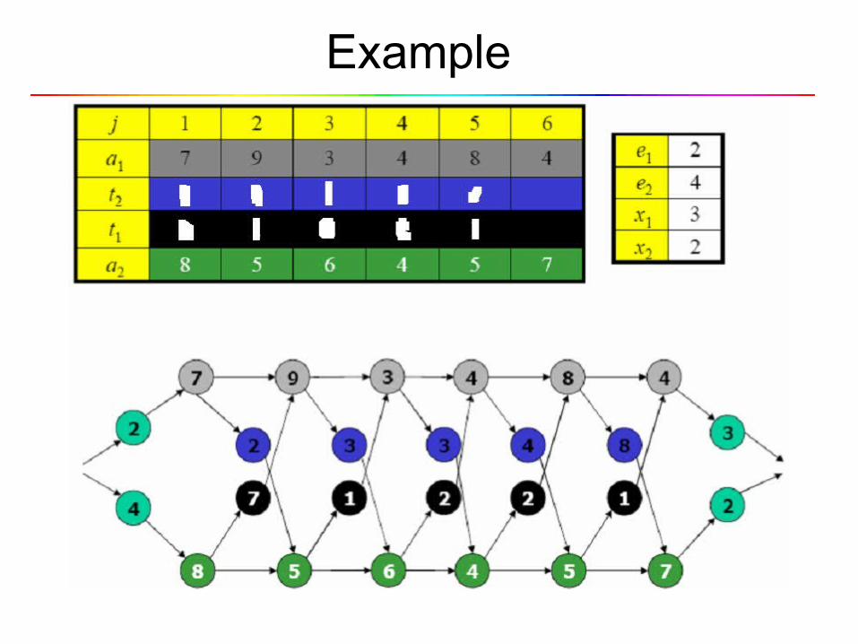
Example

Example

Step 2: Recursive Solution
• To help us keep track of how to construct an optimal solution, let us define – li[j ]: line # whose station j-1 is used in a fastest way
through Si,j (i = 1, 2, and j = 2, 3,..., n)
• we avoid defining li[1] because no station precedes station 1 on either lines.
• We also define– l*: the line whose station n is used in a fastest way
through the entire factory

Step 2: Recursive Solution
• Using the values of l* and li[j] shown in Figure (b) in next slide, we would trace a fastest way through the factory shown in part (a) as follows
– The fastest total time comes from choosing stations – Line 1: 1, 3, & 6 Line 2: 2, 4, & 5


Step 3: Optimal Solution Value

Step 3: Optimal Solution Value

Step 3: Optimal Solution Value

Step 3: Optimal Solution Value

Step 3: Optimal Solution Value

Step 3: Optimal Solution Value

Step 3: Optimal Solution Value

Step 3: Optimal Solution Value

Step 4: Optimal Solution
• Constructing the fastest way through the factory