Cosmic Matter Flux May Turn Hawking Radiation Off

Javad T. Firouzjaee1,21School of Astronomy, Institute for Research in Fundamental

Sciences (IPM), P. O. Box 19395-5531, Tehran, Iran ∗

George F R Ellis22Mathematics and Applied Mathematics Department,

University of Cape Town, Rondebosch, Cape Town 7701, South Africa†

Abstract: An astrophysical (cosmological) black hole forming in a cosmological context will besubject to a flux of infalling matter and radiation, which will cause the outer apparent horizon (amarginal trapping surface) to be spacelike [7]. As a consequence the radiation emitted close to theapparent horizon no longer arrives at infinity with a diverging redshift. Standard calculations ofthe emission of Hawking radiation then indicate that no blackbody radiation is emitted to infinityby the black hole in these circumstances, hence there will also then be no black hole evaporationprocess due to emission of such radiation as long as the matter flux is significant. The essentialadiabatic condition (eikonal approximation) for black hole radiation gives a strong limit to theblack holes that can emit Hawking radiation. We give the mass range for the black holes thatcan radiate, according to their cosmological redshift, for the special case of the cosmic blackbodyradiation (CBR) influx (which exists everywhere in the universe). At a very late stage of blackhole formation when the CBR influx decays away, the black hole horizon becomes first a slowlyevolving horizon and then an isolated horizon; at that stage, black hole radiation will start. Thisstudy suggests that the primordial black hole evaporation scenario should be revised to take theseconsiderations into account.

PACS numbers:

Contents

I. Introduction 2

II. The Eikonal approximation and the tunneling picture 4

III. The Geometric optics approximation, the wave phase, and redshift 5

IV. Eikonal approximation for cosmological black hole models 7A. Oppenheimer-Snyder collapse 7B. LTB cosmological black hole 8C. A two-fluid model 11D. Necessary and sufficient conditions 13

V. The future of the matter flux 13A. The CBR flux value 14B. The future of the CBR flux 15

VI. Exponential approximation for the affine parameter 17

VII. Discussion and Conclusions 18

References 20

A. Junction condition inside the horizon 21

∗Electronic address: j.taghizadeh.f@ipm.ir†Electronic address: gfrellisf@gmail.com

arX

iv:1

408.

0778

v2 [

gr-q

c] 6

Dec

201

4

2

B. Areal coordinate for dynamical metric 22

C. Adiabatic condition for dynamical metric 23

I. INTRODUCTION

This paper considers formation of an astrophysical black hole in a cosmological context [1]. Unlikethe simple Schwarzchild or Kerr black holes, which are static or stationary respectively, cosmologicalblack holes have dynamic behaviour and are surrounded by different kinds of matter and radiation ina changing background. In the case where the geometry is non-static, the need for a local definitionof black holes and their horizons has led to concepts such as an isolated horizon [2], Ashtekar andKrishnan’s dynamical horizon (DH) [3], and Booth and Fairhurst’s slowly evolving horizon [4]. Althoughthe different aspects of the dynamical nature of the astrophysical black hole [5] and primordial blackhole [6] have been studied, there have not been serious attempts to consider black hole particle creationin the vicinity of dynamical horizons.[51]

It was shown in a previous paper [7] that in a realistic cosmological situation, an infalling energydensity such as incoming cosmic blackbody radiation (CBR) would make the outer apparent horizon(the Outer Marginally Trapped 3-Surface, or OMOTS) become spacelike. When the apparent horizon isspacelike, it seems likely that some emitted radiation will fall into the singularity, and some will escapeto infinity. This is because the radiation is emitted in the vicinity of the apparent horizon, so some maybe emitted from far enough away that it will escape the event horizon. One might call this part of theradiation that escapes to infinity “Hawking radiation”; that is a question of terminology. We ratherrefer to all radiation from the vicinity of the apparent horizon as Hawking radiation, whether it reachesinfinity or not.

Hawking’s quantum field theory approach to black hole radiation [8, 9, 15], which applies to late timestationary black holes, is not a suitable method for calculating the Hawking temperature in the caseof a fully dynamical black hole, where one has to solve the field equations in a changing background.Even the semiclassical stress tensor approach [16] has limitations related to finding the effective actionand taking into account the backscattering problem. In such cases, one should look for alternativeapproaches allowing one to calculate the Hawking radiation in a dynamical context [11, 12, 14]. Thisradiation is plausibly emitted from the vicinity of apparent horizons rather than from near the globalevent horizon [10].

The tunneling picture of Hawking radiation emission [11, 12] suggests that when there is infallingmatter or radiation, there will be no emission of blackbody radiation arriving at future infinity from thevicinity of the OMOTS surface, because it is spacelike [7, 13]. Additionally Hawking radiation emittedfrom the inner apparent horizon (the Inner Marginally Trapped 3-Surface, or IMOTS) would have beentrapped, so on this view, no Hawking radiation would escape to infinity [13]. However this is based on aparticle picture that can be queried.

Here we show that if one uses the eikonal approximation [14], that result is confirmed: when aninfalling matter or radiation flux occurs, no Hawking radiation is emitted from the spacelike OMOTSsurface. However additionally, because of the way the phase relates to redshift, the IMOTS surface willalso not emit Hawking Radiation. In other words, both tunneling arguments (WKB approximation) [12]and eikonal arguments [10] suggest that a matter or CBR radiation flux turns off Hawking radiation toinfinity, implying that no black hole explosions [15] would occur when black holes form in a cosmologicalcontext as long as the matter flux is significant. However at very late times, all the matter that can doso will have fallen into the black hole in the ΛCDM background and the CBR will have decayed awayto almost zero. An isolated event horizon will then form and, on the eikonal view, will then lead to thestandard picture of black hole radiation.

One should note here that while the mathematically clearest derivation of the Hawking effect in theusual non-dynamical context involves calculating the evolution of the two-point function of the quantumfield backward in time from infinity to near the horizon, the relevant properties of the calculation inthat case can also be seen clearly by using the different method given in Hawking’s original paper.

3

However neither method is appropriate in the context we consider, where the semi-classical radiationwe are considering may not escape to infinity at all. That is why we use the methods we do, which aresuitable for a dynamical context. Dynamical black holes may or may not emit also Hawking radiation.This is a valid question, and we should not be using any framework that doesn’t allow it to be answeredbecause it assumes the geometry is close to Schwarzschild. The detailed discussion in most papersderiving Hawking radiation, for example [9], are confined to the case of non-dynamical black holes, andwe are considering the more realistic dynamical case. It has been suggested that the deviations fromSchwarzschild due to infalling matter would have a completely negligible effect; however this is notsupported by work on modelling dynamical black holes [5, 6].

We also consider Hawking’s original argument [8] using Bogoliubov coefficients for deriving the blackhole thermal radiation for stationary black holes (when there is no influx of matter or radiation).This argument relates radiation emission to the way the geometry of outgoing null geodesics leads toexponential rescaling of null geodesic generators of past null infinity and future null infinity [10]. Howeverwhen there is infalling matter or radiation, the fact that the OMOTS surface is spacelike causes theevent horizon to shift outwards relative to when there is no infalling energy density, and the spacetimegeometry is then such that the relevant outgoing null geodesics never reach infinity [7]: rather they fallinto the future spacelike singularity (see Fig.(6)). The Hawking argument does not then apply.

Event horizon and backreaction problem: Generally, we can divide black hole formation andevolution into three steps.

The first steps involves the gravitational collapse of matter. During this step, apparent horizons andthe singularity form, and we can define the classical event horizon. Most of the gravitational physics canbe described by classical physics. During this step, we can study the nature of the horizons (IMOTSand OMOTS) and their location, shell crossings and matter flux rate, and so on. As discussed in thispaper, the eikonal (adiabatic) approximation will not be valid during this step.

The second step is when the black hole becomes quasi-static, and we can apply the adiabatic conditionto it. The black hole starts to radiate and lose mass, and we have to consider semiclassical physicsin order to examine the time evolution [40]. During this step determining the location of the eventhorizon is complicated, because in order to find the event horizon location we need to know the wholestory of the gravitational collapse for all time. To do this, we need to solve the backreaction problem,but it seems that no one has a comprehensive theory to do so. Since the black hole at this step emitsquanta of much smaller energy than the whole mass, the adiabatic approximation used in the quantumcalculations of the emission will be valid.

The final step which determines the fate of the black hole is the quantum gravitational step. It seemsthat we can only examine the fundamental question of black hole information and the event horizonduring this step.

Our work here considers the first step – the black hole evolution – and investigates when it reachesthe second step. This argument does not cover the back reaction problem and possible eventual blackhole evaporation. To consider this, one will need to check what the effective stress-tensor associatedwith particle production is, and also that radiation emission from the central collapsing fluid [16]does not prevent formation of apparent horizons and the associated singularities [17]. These issueswill be the topic of further papers. However the tunneling approach is used by many, as is theeikonal approximation: this paper takes the argument of [7] forward by showing these two approachesagree that existence of the matter flux turns off Hawking radiation and so suppresses black hole explosions.

This paper: We will show the close relation between the eikonal approximation and particle tunnelingpicture in section II. In Section III, we discuss the eikonal approximation relation to the redshift of nullgeodesics. Section IV considers this approximation for some cosmological black hole models. In SectionV, we consider the matter and radiation flux and its evolution in time. Section VI looks at how theexponential relation between null geodesic parameters on future and past null infinities does not occurwhen the OMOTs is spacelike. We then conclude in section VII. In carrying out this study, it is convenientto think of three successive approximations. First we consider the standard case [8] with no matter fluxeffect and a static exterior spacetime. Second, we consider black holes with a constant positive influx of

4

matter or radiation at all times [7]. Finally, we consider the realistic case where the matter flux rate isnon zero at all times, but is decaying away to zero in the late time expanding universe.

II. THE EIKONAL APPROXIMATION AND THE TUNNELING PICTURE

In general relativity, the classical field φ without potential solves the massless Klein-Gordon equation

gµν∇µ∇νφ = 0. (1)

To solve it we can locally use the eikonal approximation

φ = aeiψ (2)

where the amplitude a(xi) varies much more slowly than the phase ψ(xi) when the phase ψ is rapidlyvarying: ψ 1. The eikonal approximation can be presented according to the adiabatic condition whichwill be discussed in Appendix C. Then (1) gives the eikonal equation

gµν∇µψ∇νψ = gµν∂µψ∂νψ = 0 (3)

for ψ. In analogy with a wave in Minkowski space time, ki = ∂iψ is the wave vector (here Latin indexes

run from 1 to 3) and w = −∂ψ∂t the frequency of the wave measured in the coordinate frame. For apreferred observer with four-velocity uµ, the frequency measured by the observer is w = −uµ∂µψ.

We consider the case of spherical waves: a = a(r, t), ψ = ψ(r, t). Over a small region of space time fora local observer the eikonal ψ can then be expanded to first order as

ψ = ψ0 +∂ψ

∂tt+

∂ψ

∂rr (4)

For a stationary space time the eikonal can be written

ψ = ψ0 + wt±∫ r

k(r′)dr′ (5)

where the +(-) sign in front of the integral indicates that the radial wave is ingoing (outgoing) andk(r) := kr.

The geometrical optics corresponds to the limiting case of small wavelength λ→ 0 which satisfies theeikonal equation (3). Then the eikonal equation (3) is like the Hamilton-Jacobi equation

gµν∂µS∂νS = 0 (6)

where the action S is related to the momentum by pi = ∂S∂xi

and the Hamiltonian is H = −∂S∂t . Comparingthese formula with the field case, we see that wave vector plays the same role as momentum of the particleand frequency plays the role of the Hamiltonian or energy of the particle in geometrical optics:

ki ⇔ pi, w ⇔ E ' H. (7)

To consider Hawking radiation for a dynamical black hole in the spherically symmetric case in Painleve-Gullstrand coordinates, Visser [14] has used this ansatz for the s wave:

φ = A(r, t)exp[∓i(wt−∫ r

k(r′)dr′)] (8)

which is basically the same as using (5) in (2). This form of the wave is valid provided the geometry isslowly evolving on the timescale of the wave.

On the other hand, Hartle and Hawking [28] obtained particle production in stationary black holespace-times using a semi-classical analysis which does not require knowledge of the wave modes. This

5

method has been extended to different Schwarzchild coordinates in [30]. In their method, the ratiobetween emission and absorption probabilities is given by

Γ ∼ e−βw =P[emission]

P[absorption], (9)

where the probability P is the square of the amplitude of the field: P = |φ|2. By inserting (8) in thisequation we get

Γ ∼ e−2Im∫ r k(r′)dr′ . (10)

The term∫ rk(r′)dr′ has a pole singularity on the apparent horizon and gives an imaginary part in

this coordinate system. If other coordinates had been chosen, one should have considered the temporalcontribution to the emission rate [18]. If one wants to use the particle picture for the wave and takek(r) = p(r) then we will get the emission rate in the particle picture [12]

Γ ∼ e−2Im∫ r p(r)dr = e−2ImS (11)

where S is the particle action which satisfies the Hamilton-Jacobi equation and for the Painleve coordinatesystem we have

Im

∫ r

p(r)dr = ImS. (12)

As a result, the Visser eikonal method [14] and the Parikh and Wilczek tunneling method [12] aresimilar although they have different wave and particle pictures. However there is one key difference: thetunneling method cannot apply for particle production whenever the MOTS surface is spacelike, becausethe whole concept of tunneling only makes sense for a timelike surface (where ‘inside’ and ‘outside’are well defined concepts); however the eikonal method (which is based on a wave rather than particlepicture) can give particle production when the surface is spacelike and there is slow evolution of thegeometry. This difference will be important in the sequel.

Role of the eikonal approximation: In contrast to Minkowski space time, in which the definitionof a particle with momentum k is based on a decomposition of fields into plane waves ei(wt−kx), in thedynamic case the spatial size of the wave (particle) packet varies with the dynamics of the space time, anda plane wave cannot describe it. In spacetimes with a slowly changing geometry, the so-called adiabaticvacuum allows defining a meaningful notion of particles that can be applied for an evolving space time [39].The adiabatic vacuum prescription relies on the WKB (eikonal) approximation for solutions of the waveequation. As stressed by Barcelo et.al [10], physically the adiabaticity constraint (eikonal approximation)is equivalent to the statement that a photon emitted near the peak of the Planckian spectrum should notsee a large fractional change in the peak energy of the spectrum over one oscillation of the electromagneticfield (that is, the change in spacetime geometry is adiabatic as seen by a photon near the peak of theHawking spectrum). The eikonal approximation for having particle creation may have a more profoundmeaning if we examine the quantum stress-tensor.

III. THE GEOMETRIC OPTICS APPROXIMATION, THE WAVE PHASE, AND REDSHIFT

In the vacuum (Schwarzschild) case, the event horizon is associated with infinite redshift in thefollowing sense: if a freely falling object drops into the black hole, as it approaches the event horizon,an external observer will see it with ever increasing redshift; as it crosses the event horizon, the redshiftdiverges [17]. Anywhere that Hawking radiation is associated with an event horizon [8], it is associatedwith an infinite redshift surface.

In this section we show that that association is not a coincidence: it is essential to the radiationprocess, and remains true even in the case of a dynamical horizon.

Consider the eikonal equation for the wave ϕ = A(t, r)e±iψ. It is known that kµ = ∇µψ , the normalvector of the constant phase plane, describes wave propagation, and is a null vector:

kµkµ = 0. (13)

6

Differentiating this equation gives

kµ∇νkµ = 0.

Since ∇νkµ = ∇ν∇µψ = ∇µ∇νψ = ∇µkν we get the geodesic equation

kν∇νkµ = 0. (14)

In other words, the null geodesic vector derived from the eikonal equation is affinely parametrized, andequation (13) is the same as the eikonal equation (3).

Let’s look at light propagation from an emitter (e) to an observation point (o). The frequency which

is measured by a observer with 4-velocity uµ = dxµ

dλ is w = kµuµ (λ is proper time for the time like

observer). Thus, the redshift at the observer point is

1 + z =νeνo

=(gµνk

µuν)e(gµνkµuν)o

. (15)

Note that kµ must be an affinely parametrized null vector. An infinite redshift surface is a surface suchthat the redshift of light arriving at that surface becomes infinite: (1 + z) → ∞. The geometric opticsapproximation is satisfied near an infinite redshift surface.

Let us expand the wave phase near the eikonal approximation case ψ 1:

ψ − ψ0 = ∇µψdxµ = kµdxµ

dλdλ

= νdλ = (1 + z)ν0dλ. (16)

In the second line we have used the redshift equation (15). This equation shows that the phase of thewave near the infinite redshift surface is very big: ψ 1.

According to the discussion by Visser [14], the eikonal (geometric optics) approximation is an essentialfeature for occurrence of black hole radiation. Therefore, having geometric optics valid in the closevicinity of the apparent horizon is a necessary condition for demonstrating existence of Hawking radiationby the eikonal method. We now see that we can use existence of an infinite or very large redshift surfaceas a criterion for when this is satisfied.

This is actually associated with the exponential piling up of the null affine parameter relationship onfuture null infinity that is often seen as the key to existence of Hawking radiation ([8] and see Section6). The reason is as follows: whenever there is a timelike Killing vector field ξa, the energy E of aphoton is given by E = −ξaka. On a bifurcate Killing horizon, where a Killing vector field changes fromtimelike to spacelike [24], the Killing vector parameter ξ: ξa = dxa/dξ and the geodesic affine parameterv: ka = dxa/dv are related exponentially: v = exp(κξ), κ 6= 0, which leads to the affine parameterrelationship between past and future null infinity discussed in [8]. It follows that

ka = exp(−κv)ξa, (17)

is parallely propagated on the null horizon [24], which leads to the divergent redshift relation as a nullgeodesic parallel to the horizon approaches the horizon. Note that there will be no such divergence in thecase when the Killing vector field does not change from timelike to spacelike on the horizon, but ratheris null in an open neighbourhood. This is the case when the surface gravity vanishes (κ = 0). This isthe reason that a non-zero surface gravity is a necessary condition for Hawking radiation emission [14].However of course the whole of this argument depends on the existence of the Killing vector field, and sowill not be valid in a dynamical spacetime. Our argument above can be applied in that more general case.

In the next section we consider application of the redshift condition discussed here to the case of acosmological black hole.

7

IV. EIKONAL APPROXIMATION FOR COSMOLOGICAL BLACK HOLE MODELS

The study of black holes in stationary and asymptotically flat spacetimes has led to many remarkableinsights. But, as we know, our universe is not stationary and is in fact undergoing cosmological expansionin presence of background radiation; that is the context in which we should consider gravitationalcollapse to form a black hole [7]. There have been many papers constructing solutions of the Einsteinequations representing a collapsing central mass in a cosmological context. Gluing of a Schwarzchildmanifold to an expanding FRW manifold is one such attempt, made first by Einstein and Straus [25].

Now, a widely used metric to describe gravitational collapse of a spherically symmetric dust cloudis the so-called Lemaıtre-Tolman-Bondi (LTB) metric [31]. Many people have looked at LTB modelsdescribing an overdense region in a cosmological background [1]. Although there were some attemptsto investigate Hawking radiation from dynamical black holes through tunneling [11], no one hasconsidered necessary conditions for this method in presence of a matter flux such as that due to cosmo-logical black body background radiation (CBR), which does indeed occur everywhere in the real universe.

In this section we consider the essential features of black hole radiation emission for three modelsof cosmological black holes that take this effect into account: Oppenheimer-Snyder collapse, an LTBcosmological black hole, and a two-fluid model.

A. Oppenheimer-Snyder collapse

The Oppenheimer-Snyder solution consists of a dust filled Friedmann model, joined across comovingspheres to a timelike hypersurface in the Schwarzchild solution. To make a cosmological black hole, wecan match the exterior Schwarzchild black hole to an internal spatially homogeneous FLRW universe(this is one kind of Einstein-Straus cosmological black hole). Since we want to consider the tunnelingeffect near the horizon, it is sufficient to consider an Oppenheimer-Snyder solution. The metric inside(sign -) the collapsing dust in case of a flat 3-geometry is given by

ds2− = −dτ2 + a(τ)2(dχ2 + χ2dΩ2). (18)

The Einstein equation shows that a(τ) satisfies

a2 =8π

3ρa2. (19)

The equation of conservation, ∇µTµν = 0, gives the density as ρ(τ) = ρ0a3 . We assume that at an initial

time τ = τ0 the scale factor is a = 1, then we get

a(τ) = (1− 3

2

√8πρ0

3(τ − τ0))

23 . (20)

The star surface is located at χ0 = constant. The metric outside (sign+) is given by

ds2+ = −fdt2 + f−1dR2 +R2dΩ2, (21)

where f = 1− 2M/R.

Since this coordinate system has a singularity at R = 2M , we choose the Lemaıtre coordinate [27]to give a junction with the FLRW region which does not have a coordinate singularity (see Appendix A ).

Using the junction condition one can show

M =4π

3ρa3χ3

0 (22)

which is constant. When the star radius is bigger than its Schwarzchild radius, there is no trappedsurface, i.e R > 2M . When the star falls into it’s Schwarzchild radius, there will be two parts of theapparent horizon [7]. The first on the outside is the OMOTS (Outer marginally outer trapped 3-surface)

8

which is the same as the Schwarzchild event horizon, and the second is the IMOTS (Inner marginallyouter trapped 3-surfaces) which is inside the star and reaches the singularity at R = 0. The trappedsurface is located at R = 2M which is given by

χ|AH =2M

a. (23)

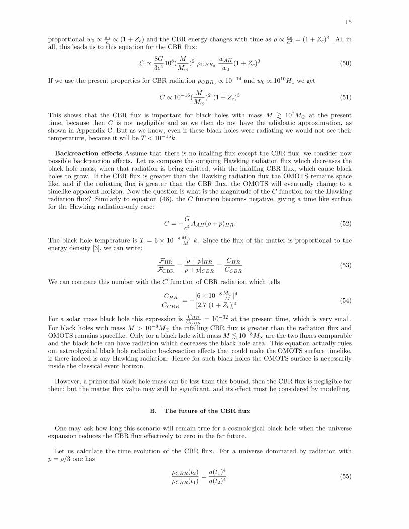
If this black hole is embedded in the cosmological CBR radiation, it will not make much difference tothe spacetime curvature, so we can treat this radiation in a linear approximation as a propagating fieldon the LTB background making little difference to the fluid collapse. It will however change the locationof the OMOTS surface, which will become spacelike because of the CBR influx, which continually fallsinto the black hole as discussed in [7, 13].

t

r

FLRW Schwarzschild

t

r

Nearly Schwarzschild

CBR

r=2M

r=0

FIG. 1: Oppenheimer-Snyder collapse in the presence of CBR and matter influx, in comoving coordinates. Theleft hand diagram is when there is no infalling flux, and the right one is for the case of a matter or radiationinflux that decays at late times.

The radiation from the vicinity of the OMOTS will be discussed in the next subsection, which is themore general case. To know whether this black hole emits radiation by tunneling from IMOTS, wehave to check the geometric optic approximation for the ingoing and outgoing null geodesics which areemitted from a point near the IMOTS, see Fig.(1). Consider an ingoing null geodesic which comes froma point (emitter) on or near the IMOTS surface and arrives at an observer outside this surface. Sincethe space time is FLRW and the IMOTS is time like: | dτdχ |null < |

dτdχ |IMOTS , the ingoing wave can pass

between the two points without an infinite change in its phase. The outgoing null geodesic can exit fromthe timelike IMOTS to outside without seeing any infinity (since the space time is FLRW).

Hence, the geometric optic approximation is not valid for ingoing or outgoing null geodesics emittednear the IMOTS. As a result, the eikonal approximation condition [14] is not valid for this surface,and there is no black hole radiation from the timelike IMOTS surface. The Penrose diagram for theOppenheimer-Snyder collapse with incoming CBR radiation is depicted in Fig.(2).

B. LTB cosmological black hole

The LTB [31] metric is a spherically symmetric non-static solution of the Einstein equations with adust source. It can be written in synchronous coordinates as

ds2 = −dt2 +R′2

1 + f(r)dr2 +R(t, r)2dΩ2. (24)

and represents a pressure-less perfect fluid satisfying

ρ(r, t) =2M ′(r)

R2R′, R2 = f +

2M

R+

Λ

3R2. (25)

9

OMOTS

IMOTS

III: + < 0

I: + > 0

SMOTS

II: + >0

CBR

Outgoing wave

OMOTS

IMOTS

III: + < 0

I: + > 0

SMOTS

II: + >0

CBR

Outgoing wave

FIG. 2: Penrose diagrams of black hole formation with incoming CBR or matter flux. The left figure is the caseof a constant infalling flux, and the right one shows the case of a decaying flux at late times. When the OMOTSsurface is spacelike because of infalling radiation, as the outgoing null wave approaches that surface, the waveredshift seen for radiation emitted from close to this surface does not diverge.

Since this metric is dynamical and includes the general case of a FLRW metric as well as inhomogeneouspressure free stars, the cosmological black hole can be modeled with this metric. As discussed in [26], wecan neglect the cosmological constant (considered as a dark energy candidate) for discussing local effectsat the black hole such as black hole horizon dynamics.

In presence of the CBR and matter flux, we assume that most of the matter inside and around theblack hole is dust causing a matter influx, and the CBR has a non-zero flux of radiation which falls inacross the horizon and which can be treated as a linear perturbation, approximated as a propagatingfield on the LTB background and making little difference to the fluid collapse. It will however changethe location of the OMOTS surface, which will become spacelike because of the CBR and matter influx[7, 13]. Thus the space time geometry can effectively be described by an LTB model embedded in thecosmological expanding background, in which the black horizon is dynamical owing to the non-zeroincoming radiation flux.

To consider the geometric optics approximation on the apparent horizon let’s look at null geodesicsnear this surface. Using the apparent horizon equation

dR = 2dM(r) = R′dr + rdt|AH , (26)

the slope of the null geodesic vector tangent to the apparent horizon tangent vector gives

dtdr |nulldtdr |AH

=R′

R′ −M ′(r)(27)

To get this equation we have used the collapsing region condition R < 0 and equation (25). Thisequation shows that if there were no matter flux into the black hole, M ′ = 0 ⇔ ρ = 0, the apparenthorizon has to be null. If the matter flux is non-zero, the slope of the null geodesic is greater than thatof the apparent horizon, which is spacelike [7]. In the case that there is no shell-crossing singularity,R′ 6=∞, and no other singularity on the apparent horizon, the null geodesics slope is finite and non-zero.

Generally the LTB apparent horizon can be either an IMOTS or OMOTS, with the nature of thelatter depending on the matter falling into the black hole [19]. In the case that the matter flux has

10

positive energy density, the OMOTS apparent horizon is spacelike and lies inside the event horizon.

No incoming CBR: It has been shown [26] that the redshift of the light emitted from the apparenthorizon for a dust BH without incoming CBR is not generically infinite, but in the case that the apparenthorizon (OMOTS) is a slowly evolving horizon it is infinite. As a result, Hawking radiation will occurfrom the OMOTS (slowly evolving horizon) for a dust cosmological black hole with no CBR.

Incoming CBR: Now we examine the redshift of the light from apparent horizons (both OMOTS andIMOTS) for a dust cosmological black hole in the presence of CBR radiation. Since the CBR radiationgives a non-zero term for the flux of the matter, it causes the black hole area to grow [3]:

F = Fmatter + FCBR :=1

G(M(r2)−M(r1))|AH , (28)

which means M ′ > 0. For this black hole, the light redshift is [26]:

1 + z = c0 exp

(−∫ e

o

R′√1 + f

dr

)

= c0 exp(

∫ e

o

−1√1 + f

(M ′

RR− MR′

RR2+

f ′

2R)dr

). (29)

CBR

t

r

e

o

CBR

t

r

e

o

R=2M (OMOTS)

R=2M (IMOTS)

o

e

o

e

FIG. 3: The LTB causal diagram near the IMOTS and OMOTS surfaces in the presence of CBR and matterinflux, in comoving coordinates.

Note that we calculate this redshift for a comoving observer uµ who is sitting at r = constant withproper time t. We can choose another observer with 4-velocity u′µ = dt

dt′uµ, and we will see that the

results will not change if there is no singularity in the second observer 4-velocity. As we know theapparent horizon is in the collapse region where R < 0 and R is finite and non-zero there. With theassumption that there is no shell-crossing singularity and no infinity for density on the apparent horizon,we get R′ and therefore M ′ is finite. As depicted in Fig.(3), the ingoing and outgoing null geodesicswhich emerge from the space like apparent horizon (OMOTS) to a point inside it, will traverse a finite∆r because dt

dr |null is finite and non-zero. Similarly, the ingoing and outgoing null geodesic which emergefrom the time like apparent horizon (IMOTS) to a point outside or inside it, will traverse a finite ∆rbecause dt

dr |null is finite and non-zero as depicted in Fig.(3). Therefore, the exponential part of theequation (29) will be finite. Hence, the cosmological black hole apparent horizon in the presence of CBRradiation and matter flux does not satisfy the geometric optics approximation. Consequently, there isno Hawking radiation from either the IMOTS surface or the OMOTS surface in this black hole. Notethat, the causal structure in the Fig.(3) does not depend on the coordinates and the apparent horizondoes not change this spacelike character, so all the above argument can be applied for other non-singularcoordinates.

This is in contrast to the Schwarzchild limit case, M ′ = 0, where there is no incoming CBR andmatter flux and the apparent horizon tangent vector is a null vector (parallel to a null geodesic).

11

Then the outgoing null geodesic traverses an infinite ∆r → ∞ from the emitter point (on the hori-zon) to the observer point (this is the essential content of equation (2.16) in [8]). Therefore, in thiscase the apparent horizon is an infinite redshift surface and there is indeed black body radiation emission.

All the above discussion can be extended to beyond the s-wave (spherical wave) case. As discussed in[14], the near-horizon asymptotic behaviour, the phase pile-up, the continuation of the outgoing modesacross horizon and Hawking temperature, are independent of having only an s-wave mode.

Even without these calculations, one can intuitively infer that since we do not have the adiabaticcondition [10] or late time apparent horizon (OMOTS) [29] for the dynamical black hole, there is noHawking radiation. This is because null radiation emitted near the apparent horizon when the CBR andmatter flux is significant would not be not tangent to the apparent horizon, which is spacelike, and sowould arrive at infinity with a finite redshift ( Fig.(2)).

C. A two-fluid model

The previous two models can be criticized because they do not model the effect on the spacetime ofthe CBR energy density. Here we consider a 2-fluid model representing the dynamic effects of both thematter and the CBR radiation. As the latter is isotropic to very high accuracy in a FLRW model, we canrepresent it as a perfect fluid with 4-velocity uaCBR, density ρCBR, and pressure pCBR = 1

3ρCBR. Thusthe first fluid is ordinary matter fluid (non-zero inside the collapsing fluid, zero outside,) and the secondone is the CBR radiation fluid. We assume the matter flux to be a perfect fluid, which can representa realistic picture of gravitational collapse [33] and has the ability to model a cosmological black hole [26].

It can be shown that the sum of the two perfect fluids is a fluid with anisotropic stress πab and heat flowqa [32]. However we can set the heat flow to zero by choosing the timelike vector ua as the eigenvector ofthe Ricci tensor: then qa = 0. Because of the spherical symmetry of the problem, we can represent theanisotropic fluid pressure in this frame by two terms: a radial pressure pr and a tangential pressure pθ.For slowly moving matter relative to the CBR, this effective fluid has

ρ = ρm + ρCBR. (30)

The collapsing fluid within a compact spherically symmetric spacetime region will be described by thefollowing metric in the comoving coordinates (t, r, θ, ϕ):

ds2 = −e2ν(t,r)dt2 + e2ψ(t,r)dr2 +R(t, r)2dΩ2. (31)

The energy momentum tensor for the fluid will have the form

T tt = −ρ(t, r), T rr = pr(t, r), T θθ = Tϕϕ = pθ(t, r), (32)

with the weak energy condition satisfied:

ρ ≥ 0 ρ+ pr ≥ 0 ρ+ pθ ≥ 0. (33)

The Einstein equations give,

ρ =2M ′

R2R′, pr = − 2M

R2R, (34)

ν′ =2(pθ − pr)ρ+ pr

R′

R− p′rρ+ pr

, (35)

− 2R′ +R′G

G+ R

H ′

H= 0, (36)

12

where

G = e−2ψ(R′)2 , H = e−2ν(R)2, (37)

and M is Misner-Sharp mass defined by

G−H = 1− 2M

R. (38)

As discussed in [26], the surface R = 2M is the apparent horizon for the collapsing region. In this casethe matter flux which falls into the singularity is,

F = Fmatter + FCBR :=1

G(M(t2, r2)−M(t1, r1))|AH , (39)

As a result of non-zero CBR and matter flux, the density and the pressure are finite on the apparenthorizon and then there are non-zero and finite values for M ′ > 0, M > 0. No shell-focusing singularity,no shell-crossing singularity and the apparent horizon location in the collapsing region give non-zero andfinite values for R, R′ and R < 0 on the apparent horizon respectively. The null geodesic slope on the

apparent horizon is dtdr |null = ± R′

|R| which according to the above discussion is finite for the outgoing and

ingoing null geodesics. With some calculation one can get following equation on the horizon

dtdr |nulldtdr |AH

=

(1− 2M

R

1− 2M ′

R′

). (40)

In the vacuum (Schwarzchild limit) case M ′ = 0 ⇔ ρ = 0 and M = 0 ⇔ p = 0, so the apparent horizon

becomes a null surface. Using the weak energy condition (33) we get 2M ′

R′ ≥2MR

. The case of equality

in the weak energy condition ρ = −p is very special and non applicable to a realistic cosmological blackhole, so we get

2M ′

R′>

2M

R. (41)

Using this equation in (40) results in the dynamical case where the null geodesics cross the apparenthorizon (which is spacelike [7]), and for the outgoing null geodesic we have

dtdr |nulldtdr |AH

> 1. (42)

In this way we can calculate the light redshift from the apparent horizon of this metric. To this end, weneed to calculate the affine parametrized radial null geodesic vector kµ. Without writing the details ofthe calculation, the result is that the affinely parametrised null vector is

kµ = c0e−

∫(ν+ψ+ν′eν−ψ) dr

eν−ψ (1,R

R′, 0, 0) (43)

Considering a comoving observer with uµ = (e−ν , 0, 0, 0), we can calculate the redshift of the null geodesicsfrom the emitter point to the observer point. Using the geometric optics approximation, the question is

whether the quantity e−∫(ν+ψ+ν′eν−ψ)dt is infinite on the apparent horizon. Let us check all terms in this

equation. The term eν−ψ = RR′ on the horizon, which is finite. We rewrite the equation (38) as

M =R

2(1− e−2ψ(R′)2 + e−2ν(R)2). (44)

The time derivative of this equation shows that if ν and ψ are infinite, then M will be infinite, which asdiscussed above is an unphysical condition on the horizon. Finally, with non-singularity of the pressureon the horizon, equation (35) says that ν′ is finite. Overall, there is no infinity for the redshift of the nullgeodesic coming from the apparent horizon. Following the last section’s discussion, there is no eikonalapproximation for the null geodesics coming from apparent horizon (both OMOTS and IMOTS), andhence no emission of Hawking radiation.

13

D. Necessary and sufficient conditions

As pointed out by Visser [14], there are two other essential conditions for having black hole radiationfor a Lorentzian metric beside the eikonal approximation: the first is existence of an apparent horizon,and the second is non-zero surface gravity.

As regards the apparent horizon, its existence is necessary for defining the black hole boundary indynamical collapse [3]. The Oppenheimer-Snyder (OS) model has an apparent horizon that consists oftwo parts, the IMOTS and the OMOTS [7]. For the LTB gravitational collapse model, it was shownin [1, 26] that an apparent horizon will form at R = 2M after some time, and every LTB gravitationalcollapsing model has an apparent horizon. For the third (two-fluid) model of gravitational collapse, thescenario is different, because in such a model the gradient of the pressure acts as a repulsive force andcan in principle prevent formation of the apparent horizon. However this depends on the details of thegravitational collapse such as the equation of state [33, 41], and for realistic equations of state a blackhole will result if the initial mass of the collapsing object is large enough [27, 42]. For studying blackhole radiation in the general spherically symmetric case, the surface R = 2M is again the black holeboundary, which is an apparent horizon.

The surface gravity definition for the first (OS) model is trivial. But the surface gravity definition fora general dynamical metric is not trivial. Having a covariant definition for quantities in thermodynamicsis very important because our physical quantities should not depend on the coordinates that we use tocalculate. Fortunately, there is nice formula for the thermodynamic law in the spherically symmetric case[43] where the temperature is proportional to the surface gravity. The surface gravity definition of [14]was rewritten in a covariant formalism in the spherically symmetric black hole case in [11]. As shown in[44], and we calculate in equation (C4) for the LTB metric, the surface gravity is non-zero for sphericallysymmetric dynamical black holes.

V. THE FUTURE OF THE MATTER FLUX

As we have noted, the spacelike nature of apparent horizon (coming from the in-falling matter orradiation flux) causes light to pass it without having infinite redshift. Let us quantify this property.Consider the future-directed outgoing and ingoing null normals la and na respectively at a point, andthe expansions θ` and θn of the congruences of curves generated by these vector fields.

Let V a be tangential to H (the MOTS hypersurface in Fig.(4)), and orthogonal to the foliation bymarginally trapped surfaces. It is always possible to find a function C and normalization of `a such thatV a = `a−Cna. In addition, the definition of V a implies that LV θ` = 0, which gives an expression for C:

C =L`θ`Lnθ`

. (45)

When C < 0 the apparent horizon is an IMOTS and C > 0 the apparent horizon is an OMOTS, andif C = 0 it becomes an event (isolated) horizon. The value for the C function is important because itshows the type of the black hole horizon. It shows if a MOTS surface is an OMOTS or IMOTS surfaceand whether it is timelike or spacelike (see Section 1.2 and Table 1 in[13]), and specially, as discussed inthe Appendix C, it is a criterion for where the adiabatic approximation is satisfied.

As discussed in [19], in the case of perfect fluid collapse C ∝ (ρ+p) on the horizon. To see its behaviourlet us look at the Friedmann equation for the standard model of a ΛCDM universe with FLRW metric

(a

a)2 =

8πG

3ρ+

Λ

3, (46)

where energy conservation is

ρ+ 3(ρ+ p)a

a= 0. (47)

The background matter density dilutes as ρm = ρma3 . On the other hand, we know in the expanding

background, only part of matter around the black hole can fall into it. For instance, for a de Sitter universe

14

representing the late evolution of a ΛCDM model, there is a cosmological event horizon. Therefore, aftersome time the black hole devours all the available matter around itself and after that there is no matterflux which can make the apparent horizon a spacelike surface, i.e C → 0. Note that this is a roughapproximation because the matter around the black hole has pressure and the matter energy densityincreases when it gets near the black hole horizon, so in a more realistic model, C is greater than thisapproximation and one needs a black hole simulation to find it.

R

Isolated horizon

OMOTS

flux

ℓ n

V

particle

antiparticle

FIG. 4: Particle creation and annihilation around the apparent horizon for the case if an influx that decays awayat late times. The OMOTS surface starts at an SMOTS 2-sphere (bottom) and is first spacelike and dynamical;at this stage virtual particle pairs can annihilate, and no radiation results. It then becomes first a slowly evolvinghorizon, and then at very late times an isolated horizon. At this stage virtual particle pairs can be separated bythe OMOTS apparent horizon, and radiation results. Note that we did not include radiation backreaction in thisFigure, which is adapted from arXiv:gr-qc/0308033.

A. The CBR flux value

In the last subsection we did not consider the CBR radiation. As discussed above, the C function (45)is a criterion for a MOTS surface being spacelike [13, 34]. To calculate the radiation flux we considerthe CBR as a null fluid that moves inwards from infinity towards the center. In this case Booth [19] hasshown that the C function is

C =2G

c4AAH(ρ+ p) (48)

where AAH is apparent horizon area. At first sight, it seems that C is very small for the current CBRenergy density ρCBR ' 10−14 J/m3, but the basic point is that we have to calculate this energy densityon the horizon, when CBR photons come from a large distance and get to the horizon. Therefore, the Cfunction is

C =8G

3c4AAH ρCBR

wAHwbackground

(49)

where the w is the CBR photon frequency for Kodama observers [8]. As shown in the Appendix B, forKodama observers (which reduce to static observers in the static case as discussed ref [8]), the CBRphoton frequency becomes infinitely blue shifted when it gets to the apparent horizon. The infinitycannot have any meaning in classical physics. This is the trans-Planckian problem [35] which says thatat the very onset of the formation of the trapping horizon, we must consider semiclassical physics. Wecan roughly use the Planckian cutoff frequency to estimate the value of wAH , which is 1043Hz. Let uspresent the general formula for a black hole with mass M and at cosmological redshift time 1 +Zc = a0

a(t)

(the usual time scale in astronomy and cosmology). We know that the CBR background frequency is

15

proportional w0 ∝ a0a ∝ (1 + Zc) and the CBR energy changes with time as ρ ∝ a0

a4 = (1 + Zc)4. All in

all, this leads us to this equation for the CBR flux:

C ∝ 8G

3c4108(

M

M)2 ρCBR0

wAHw0

(1 + Zc)3 (50)

If we use the present properties for CBR radiation ρCBR0 ∝ 10−14 and w0 ∝ 1010Hz we get

C ∝ 10−16(M

M)2 (1 + Zc)

3 (51)

This shows that the CBR flux is important for black holes with mass M & 107M at the presenttime, because then C is not negligible and so we then do not have the adiabatic approximation, asshown in Appendix C. But as we know, even if these black holes were radiating we would not see theirtemperature, because it will be T < 10−15k.

Backreaction effects Assume that there is no infalling flux except the CBR flux, we consider nowpossible backreaction effects. Let us compare the outgoing Hawking radiation flux which decreases theblack hole mass, when that radiation is being emitted, with the infalling CBR flux, which cause blackholes to grow. If the CBR flux is greater than the Hawking radiation flux the OMOTS remains spacelike, and if the radiating flux is greater than the CBR flux, the OMOTS will eventually change to atimelike apparent horizon. Now the question is what is the magnitude of the C function for the Hawkingradiation flux? Similarly to equation (48), the C function becomes negative, giving a time like surfacefor the Hawking radiation-only case:

C = −Gc4AAH(ρ+ p)HR. (52)

The black hole temperature is T = 6 × 10−8MM k. Since the flux of the matter is proportional to theenergy density [3], we can write:

FHR

FCBR=

ρ+ p|HRρ+ p|CBR

=CHRCCBR

(53)

We can compare this number with the C function of CBR radiation which tells

CHRCCBR

= −[6× 10−8MM ]4

[2.7 (1 + Zc)]4(54)

For a solar mass black hole this expression is CHRCCBR

= 10−32 at the present time, which is very small.

For black holes with mass M > 10−8M the infalling CBR flux is greater than the radiation flux andOMOTS remains spacelike. Only for a black hole with mass M . 10−8M are the two fluxes comparableand the black hole can have radiation which decreases the black hole area. This equation actually rulesout astrophysical black hole radiation backreaction effects that could make the OMOTS surface timelike,if there indeed is any Hawking radiation. Hence for such black holes the OMOTS surface is necessarilyinside the classical event horizon.

However, a primordial black hole mass can be less than this bound, then the CBR flux is negligible forthem; but the matter flux value may still be significant, and its effect must be considered by modelling.

B. The future of the CBR flux

One may ask how long this scenario will remain true for a cosmological black hole when the universeexpansion reduces the CBR flux effectively to zero in the far future.

Let us calculate the time evolution of the CBR flux. For a universe dominated by radiation withp = ρ/3 one has

ρCBR(t2)

ρCBR(t1)=a(t1)4

a(t2)4. (55)

16

In the case of a matter dominated universe this term becomes

ρCBR(t2)

ρCBR(t1)=

(t1)8/3

(t2)8/3(56)

while in the dark energy dominant era it is

ρCBR(t2)

ρCBR(t1)= e4H(t1−t2) (57)

where H = aa . The present value of the Hubble expansion rate is H0 = 3.241 × 10−18hs−1 where

h ' 0.72 ± 0.1. As discussed in last subsection, if we assume that the C value decreases 2 ordersof magnitude and OMOTS becomes nearly a null surface relative to the cosmological frame, thisapproximately means that the energy density decrease 2 orders of magnitude (the C function is keyto the validity of adiabatic condition (see Appendix C), hence we can use it to find approximatelywhen the black hole radiation will start.) One can easily see that the times when the energy densityof the CBR decreases to 1

100 of that at the present time in these two models are t2 ' 2.44 × 1018s

and t2 ' 7 × 1017s from the present time respectively. Similar calculations can be done for the matterflux. Therefore, we can say that the CBR and matter flux effect effectively cannot be diluted by thecosmological expansion in the short term. In the other words, these calculations show that the cosmologi-cal expansion is not significant in turning off the matter and CBR flux on cosmologically short time scales.

However, leaving aside strange behaviour such as dynamical dark energy, cosmological particlecreation, and big crunch singularity models, this picture says that at very large times there is effectivelyno CBR flux. Although it never becomes exactly null or timelike ([7], section VIII.2), the OMOTSeventually becomes an isolated horizon that is very close to the classical event horizon. HawkingRadiation emission could occur from that time on as depicted in Fig.(5), because the approximations wehave used above in the eikonal analysis would break down at that stage, with associated backreactioneffects and possibly eventual black hole evaporation.

CBR

No CBR flux only Hawking radiation

Event horizon

Apparent horizon

Future infinity BH singularity

FIG. 5: Penrose diagram for a black hole in a ΛCDM expanding universe, where there is a matter and radiationinflux, but it dies away to zero in the far future. Note that we do not represent back reaction effects in this picture.

This is the key difference from the particle approximation and associated tunneling picture, becauseon that view, there would never be Hawking radiation emission, as the OMOTS surface would always bespacelike, so no Hawking Radiation backreaction effects or black hole evaporation would occur even inthe very far future.

17

VI. EXPONENTIAL APPROXIMATION FOR THE AFFINE PARAMETER

This paper so far has been based on examining the Eikonal approximation and its implications.However the original calculation by Hawking [8] was based on the way that the affine parameters on pastnull infinity I− and future null infinity I+ are related to each other by an exponential transformation,so an infinite range of the parameter v on I− corresponds to a finite range of the parameter u on I+(see Figure 4 of [8]). Following this, in order to find the minimal condition for having thermal-like blackhole radiation, Visser et al [10] have shown that any collapsing compact object (regardless of whetheror not any type of horizon ever forms) will emit a slowly evolving Planckian flux of quanta, providedthe adiabatic condition and exponential approximation hold along the null congruence which travelsfrom past null infinity to future null infinity. Having such a relation for wave packets and applying thestandard Hawking calculation [8] to derive time-dependent Bogoliubov coefficients, we can see this givesus a Planckian spectrum with a time-dependent Hawking temperature. Thus it was shown there thatthe exponential relation between the affine parameters on past null infinity, vin, and future null infinity,uout, is the necessary and sufficient condition for generating a Hawking flux.

In the case of black hole formation in a vacuum context, this leads to Hawking’s picture. Howeverin the case of a spacelike dynamical horizon as considered in this paper, the pile up of the u-parameterrelative to the v-parameter does not reach infinity, because the OMOTs is spacelike (see Fig.(6)). Therelevant null geodesics (for u → ∞) cross the apparent horizon (the OMOTS surface) and do not reachfuture null infinity [7]. The null coordinate u does not tend to infinity there, and hence surfaces ofconstant w of the solution pw will not pile up at this surface as in the vacuum case considered byHawking ([8], just after Fig 4).

III

Event Horizon

OMOTS

Future Singularity

IMOTS

I

II

FIG. 6: Penrose diagram for black hole formation with incoming radiation that does not decay away. A spacelikeOMOTS surface means the infinite affine parameter rescaling between ingoing and outgoing null geodesics thatoccurs in the pure vacuum case ([8], Fig. 4) does not reach infinity: it is trapped by the singularity.

Putting this in the LCDM context where future infinity is spacelike [7], although there is a unique

18

event horizon which is the inmost event horizon associated with the black hole, as the CBR becomescooler and cooler, asymptotically the OMOTS will (in the preferred cosmological frame) tend to beingnull from being spacelike, but will never actually become null (Fig.(5)). It is then a delicate issue of howthe limits work as to whether black hole radiation results from the null geodesics which pass near theslowly evolving horizon at very late times.

One might be concerned that neither the WKB approximation nor apparent horizons are necessaryfor the Hawking effect, see [40] and [45]. The point however is that we don’t consider the most generalfeatures of spherical collapse and Hawking radiation. We look for the Hawking radiation phenomenon inthe case of cosmological black holes which do indeed have apparent horizons [7]. We also have used thetunnelling approach [11, 12, 14, 30], for which the WKB approximation is a necessary assumption. Asshown above, this means that we need a surface that has a very large redshift (not necessarily infinite)for the received light that is emitted from near the apparent horizon, and this leads to our results. Inaddition, to check the outcome, we have applied the adiabatic condition for cosmological black holes inAppendix C, which is another approach that confirms our results.

VII. DISCUSSION AND CONCLUSIONS

There are several effects related to the vacuum in quantum field theory: the zero point energy,Casimir effect, and dynamical Casimir effect (which is like a moving mirror). There are three morequantum vacuum effects that are due to a curved spacetime: metric quantum fluctuations, vacuumpolarization, and Hawking particle creation [27]. Particle creation results from the Hawking particlecreation effect and dynamical Casimir effect (or moving mirror). Basically, Hawking particle creationis thermal radiation due to the black hole horizon which is observed at a large distance. On the otherhand, the dynamical Casimir effect is the production of particles and energy from an accelerated movingmirror (see [46] for a comprehensive review). The question is how we can see this effect in a curvedspace time or in black hole collapse. In a flat space time, the dynamical Casimir effect appears due toa special boundary condition for wave solutions. We can include this effect in a curved space time bysolving the general wave equation (including backscattering and boundary conditions) and finding theappropriate vacuum for it (which is like an initial condition). Hence, we can see traces of this effect inthe expectation value of energy momentum tensor < Tµν > as vacuum polarization [22].

In our dynamical spherically symmetric space time where the apparent horizon is inside the eventhorizon, any virtual pair particle created due to these effects cannot fall outside the event horizon,become real, and reach future infinity; however it can be seen locally in < Tµν > inside horizon. Butfor any general realistic model of star collapse, we must first solve the wave equation with suitableboundary conditions (the dynamical Casimir effect has dynamical boundary conditions) and second findthe appropriate vacuum corresponding to the collapsing model (like the Unruh vacuum), and only then

can we read the general particle creation occurring from the number density operator < N = a†kak > and< Tµν >. It seems that in the analogue gravity models for Hawking radiation, we can see the dynamicalCasimir effect [47]. One can consider collapsing star models with special dynamical boundary conditionto probe the dynamical Casimir effect for particle creation, which is beyond the scope of this paper.Here we just discuss the blackbody particle creation due to Hawking radiation.

We have shown that when one uses either the tunneling approximation [12], [11] or the eikonal approx-imation [14], one finds that turning on the CBR and matter flux turns off the Hawking radiation emissionfrom the OMOTS surface, and there is also no such radiation emitted from the IMOTS surface. The keyfeature leading to this result is shown in the contrast between the two cases in Fig.(1) and Fig.(5):

• When we have the vacuum case outside the star, the OMOTS surface coincides with the null eventhorizon. Radiation emitted close enough to this surface reaches infinity with an unboundedly largeredshift. It is this divergent redshift that is the reason Hawking radiation is emitted just outsidethe null OMOTS surface and escapes to infinity. The ultimate source of the divergent redshift isthe infinite rescaling that takes place between the affine parameter and the group parameter ona bifurcate Killing horizon [24] (cf. equation (2.16) in [8]); hence it is a consequence of the staticnature of the exterior vacuum solution, which allows this symmetry group.

• When we take into account the infalling CBR radiation and matter flux, Fig.(5), the OMOTS

19

surface is spacelike and lies inside the null event horizon [7]. Outgoing rays reaching infinity fromjust inside its classical event horizon, or emitted inside that horizon but outside the OMOTS surface,no longer experience this unbounded redshift; and the same applies to the IMOTS surface. That isthe reason that no Hawking radiation is emitted in this case.

This is related to the fact that when the flux falls into the black hole, it’s mass increases, hence thisis no longer a quasi-static spacetime and there is no external Killing vector field with an associatedbifurcate Killing horizon. The conclusion is reinforced by the fact that there will be many otherkinds of radiation and matter that will also fall into an astrophysical black hole, and increase itsmass further. This is a self consistent approximation: as long as there is CBR and matter influx,the OMOTS surface will remain spacelike at all times because there is no incoming negative densityHawking radiation that could make it timelike [7].

• As depicted in Fig.(5), in the particle tunnelling scenario, if a pair of a particle and antiparticleare created near the dynamical horizon, both of them will fall into the singularity and annihilateeach other, so no Hawking radiation will be emitted. However a particle created near an isolatedhorizon or slowly evolving horizon can reach future infinity, and Hawking radiation will occur. Onthe other hand, since the geometric optics approximation does not generally held near the OMOTS,we cannot apply the particle interpretation for this surface.

• At a late enough time in the very far future, the cosmological expansion decreases the CBR andmatter density and black hole will devour all the available matter around itself. The black holehorizon then becomes first a slowly evolving horizon [4] and then an isolated horizon [2] Fig.(5).Black body radiation could then initiate at that stage, and possibly lead to black hole explosionsat a later time.

• As long as the matter flux into the black hole is not negligible there is no Hawking radiation, butthe black hole radiation scenario is currently applied to every dynamical black hole. However, allblack holes in the real universe are surrounded by different types of matter and radiation leading tosubstantial positive density energy influx for much of their life, and particularly in the very earlyuniverse.

• Application of this constraint to primordial black hole evaporation modelling may bring in a correc-tion to their abundance in the cosmos. Specifically, primordial black holes are candidate progenitorsof unidentified Gamma-Ray Bursts (GRBs) that are supposed to detect by the Fermi Gamma-raySpace Telescope observatory. Their abundance might be lowered when the above considerations aretaken into account.

This is all in accord with the discussions in [7, 13], and leads to the conclusion that in a realisticcosmological context, a black hole forming from the collapse of a star in a universe permeated by CBRand matter will not emit Hawking radiation in the past or at the present, and so emission of suchradiation from them, or evaporation of such black holes in an explosion, will not occur in the visibleuniverse. To what degree this affects primordial black holes, or thefar future universe, will be verycontext dependent and will need detailed modelling.

One should contrast the above with the Parikh and Wilczek tunnelling method (in standard generalrelativity) [12], which cannot apply for particle production whenever the OMOTS surface is spacelike,because the whole concept of tunnelling only makes sense for a timelike surface, where ‘inside’ and‘outside’ are well defined concepts (see [12]: paragraphs just after eqn. (8)). Therefore, the tunnellingpicture is only applicable from the moment that the instantaneous Hawking radiation flux is greaterthan the matter flux and the black hole apparent horizon becomes a timelike surface.

Generally, in broader contexts, we cannot say that the tunnelling method requires the apparenthorizon to be timelike, due to particle creation by tunnelling. One can apply this method even forspacelike universal horizons in Einstein-aether theory [48, 49] which has a non-standard causal structure.Note also that the adiabatic approach does not limit the horizon to be a timelike or spacelike surface.The point is that the adiabatic condition can be satisfied for an apparent horizon that becomes spacelikedue to the CBR flux. In addition, in our models, we quantify the WKB condition in the tunnellingmethod as the light redshift from the horizon, which is not a comprehensive approach. One can quantifythis as the width of the horizon in order to calculate the lingering time in acoustic black holes or

20

Lorentz-invariance violating models [49, 50].

As mentioned above and emphasized in [7], this work should be extended in two significant ways:

• By calculating the expectation value of the stress tensor in this scenario (cf. [16]),

• By checking that radiation emission from within the collapsing fluid does not prevent horizonformation by back reaction of emitted Hawking Radiation, as has been suggested in [38]. Thatcalculation would be altered in the cosmological context considered here, where inter alia theHartle-Hawking vacuum is not the appropriate vacuum state to use, and the spacelike nature of theOMOTS surface will modify the way modes propagating through the collapsing fluid [8, 16] reachinfinity.

However in terms of calculation methods that are used by various authors for determining the extentof Hawking radiation emission, the result given here seems conclusive. Note that we do not claim toprove that no radiation at all will be emitted. The break down of the adiabatic approximation impliesonly absence of a Planckian spectrum, not necessarily of any radiation. Indeed, a rapidly evolvingapparent horizon would most probably lead to some form of particle production with typical frequenciesexcited of the order of the inverse timescale of the evolution of the metric (maybe linked to the accretionrate). This is a (geometrically induced) Dynamical Casimir effect, which per se can be far from thermalin character but not necessarily negligible (because the time dependence of the apparent horizon issupposed to be fast/non-adiabatic in the early universe).

Acknowledgments:

We thank Malcolm Perry and Reza Mansouri for fruitful discussions, and Ritu Goswami, Tim Clifton,David Jacobs and Matt Visser for helpful comments on an earlier version of this paper, as well asa referee for useful comments. We thank the National Research Foundation (South Africa) and theUniversity of Cape Town Research Fund for support.

[1] A. Krasinski and C. Hellaby, Phys. Rev. D 69, 023502 (2004); W. Valkenburg, Gen.Rel.Grav. 44 (2012)2449-2476;C. Gao, X. Chen, Y-G. Shen and V Faraoni, Phys.Rev. D84 (2011) 104047; J. T. Firouzjaee, RMansouri, Gen. Rel. Grav. 42, 2431 (2010); K. Bolejko, M-N. Celerier and A. Krasinski, Class.Quant.Grav.28 (2011) 164002; J. T. Firouzjaee, M. Parsi Mood and R. Mansouri, Gen. Rel. Grav. 44, 639 (2012).

[2] A. Ashtekar, C. Beetle, O. Dreyer, S. Fairhurst, B. Krishnan, J. Lewandowski and J. Wisniewski, Phys. Rev.Lett. 85, 3564 (2000).

[3] A. Ashtekar and B. Krishnan, Phys. Rev. Lett. 89, 261101 (2002); A. Ashtekar and B. Krishnan, Phys. Rev.D 68, 104030 (2003).

[4] I. Booth and S. Fairhurst, Phys. Rev. Lett. 92, 011102 (2004)[5] A. Ashtekar and B. Krishnan, Living Rev. Rel. 7, 10 (2004); J. L. Jaramillo, R. P. Macedo, P. Moesta and

L. Rezzolla, Phys. Rev. D 85, 084030 (2012).[6] T. Harada and B. J. Carr, Phys. Rev. D 71, 104010 (2005); D. C. Guariento, J. E. Horvath, P. S. Custodio

and J. A. de Freitas Pacheco, Gen. Rel. Grav. 40, 1593 (2008); I. Musco, J. C. Miller and L. Rezzolla, Class.Quant. Grav. 22, 1405 (2005).

[7] G F R Ellis, R Goswami, A I. M. Hamid and S D. Maharaj arXiv:1407.3577 [gr-qc].[8] S W Hawking (1975) Comm Math Physics 43: 199-220.[9] S. Hollands and R. M. Wald, arXiv:1401.2026 [gr-qc].

[10] C. Barcelo, S. Liberati, S. Sonego and M. Visser, JHEP 1102, 003 (2011); C. Barcelo, S. Liberati, S. Sonegoand M. Visser, Phys. Rev. D 83, 041501 (2011)

[11] R. Di Criscienzo, S. A. Hayward, M. Nadalini, L. Vanzo and S. Zerbini, Class. Quant. Grav. 27, 015006(2010); J. T. Firouzjaee and R. Mansouri, Europhys. Lett. 97, 29002 (2012)

[12] M. K. Parikh and F. Wilczek, Phys. Rev. Lett. 85, 5042 (2000).[13] G. F R Ellis, arXiv:1310.4771 [gr-qc].[14] M. Visser, Int. J. Mod. Phys. D 12, 649 (2003).[15] S W Hawking (1974) Nature 248, 30–31.[16] N D Birrell and P C W Davies (1984) Quantum Fields in Curved Space (Cambridge: Cambridge University

Press)

21

[17] S W Hawking and G F R Ellis (1973) The Large Scale Structure of Space-Time (Cambridge: CambridgeUniversity Press).

[18] E. T. Akhmedov, T. Pilling, and D. Singleton, Int.J.Mod.Phys.D17:2453-2458, (2008) ; V. Akhmedova, T.Pilling, A. de Gill, and D. Singleton, Phys. Lett. B 666 (2008) 269 .

[19] I. Booth, L. Brits, J. A. Gonzalez and C. Van Den Broeck, Class. Quant. Grav. 23, 413 (2006) [gr-qc/0506119].[20] R H Boyer (1969) Proc. R. Soc. Lond. A:311 245-252.[21] T Clifton (2008) Class.Quant.Grav. 25:175022 [arXiv:0804.2635][22] P. C. W. Davies (1976) Proc Roy Soc (London) 351: 129-139.[23] P C W Davies, S A Fulling, and W G Unruh, Phys. Rev. D13, 2720 (1976) .[24] R. H. Boyer (1969) Proc. R. Soc. Lond. A 311:245-252[25] A. Einstein and E.G. Straus, Rev. Mod. Phys. 17, 120 (1945)[26] J. T. Firouzjaee, Int. J. Mod. Phys. D 21, 1250039 (2012)[27] V. P. Frolov and I. D. Novikov, Black hole physics: basic concepts and new developments, Kluwer Academic

Publishers, Dordrecht 1998.[28] J.B. Hartle and S.W. Hawking, Phys. Rev. D 13, 2188 (1976).[29] P. Hajicek, Phys. Rev. D 36, 1065 (1987)[30] S. Shankaranarayanan, T. Padmanabhan and K. Srinivasan, Class. Quant. Grav. 19, 2671 (2002).[31] R. C. Tolman, Proc. Natl. Acad. Sci. U.S.A. 20, 410 (1934); G. Lemaıtre, Ann. Soc. Sci. Bruxelles I A53, 51

(1933); H. Bondi, Mon. Not. R. Astron. Soc. 107, 343 (1947); K Bolejko, A Krasinski, C W Hellaby and M-NClrier, Structures in the Universe by Exact Methods - Formation, Evolution (Cambridge University Press,2009)

[32] G F R Ellis, R Maartens and M A H MacCallum, Relativistic Cosmology (Cambridge University Press).[33] P. S. Joshi, Gravitational Collapse and Spacetime Singularities (Cambridge University Press).[34] W. Kavanagh and I. Booth, Phys. Rev. D 74, 044027 (2006).[35] T. Jacobson, Phys. Rev. D 48, 728 (1993); L. C. Barbado, C. Barcelo, L. J. Garay and G. Jannes, JHEP

1111, 112 (2011).[36] H. Kodama, Prog. Theor. Phys. 63, 1217 (1980).[37] A. B. Nielsen and J. T. Firouzjaee, Gen. Rel. Grav. 45, 1815 (2013).[38] L Mersini-Houghton, arXiv:1406.1525 [hep-th][39] L. Parker, Phys. Rev., 183, 1057 (1969).[40] C. Barcelo, S. Liberati, S. Sonego and M. Visser, Phys. Rev. D 77, 044032 (2008) .[41] R. Moradi, J. T. Firouzjaee and R. Mansouri, arXiv:1301.1480 [gr-qc].[42] C W Misner, K S Thorne and J A Wheeler (1973) Gravitation (Freeman).[43] S. A. Hayward, Class. Quant. Grav. 15, 3147 (1998).[44] M. Pielahn, G. Kunstatter and A. B. Nielsen, Phys. Rev. D 84, 104008 (2011).[45] M. Smerlak and S. Singh, Phys. Rev. D 88, no. 10, 104023 (2013).[46] Michael Bordag, Galina Leonidovna Klimchitskaya, Umar Mohideen, and Vladimir Mikhaylovich Mostepa-

nenko, Advances in the Casimir Effect (Oxford University Press).[47] C. Barcelo, S. Liberati and M. Visser, Living Rev. Rel. 8, 12 (2005) [Living Rev. Rel. 14, 3 (2011)]; I. Caru-

sotto, S. Fagnocchi, A. Recati, R. Balbinot and A. Fabbri, New J. Phys. 10, 103001 (2008).[48] P. Berglund, J. Bhattacharyya and D. Mattingly, Phys. Rev. Lett. 110, no. 7, 071301 (2013).[49] B. Cropp, S. Liberati, A. Mohd and M. Visser, Phys. Rev. D 89, 064061 (2014).[50] S. Finazzi and R. Parentani, Phys. Rev. D 83, 084010 (2011).[51] It has been commented that horizons (whether apparent horizons or event horizons) do not somehow “emit-

ted” particles/radiation because quantum field theory in curved spacetime does not describe the Hawkingprocess in this manner at all. But in our view this is just semantics. There are papers that show that theradiation appears to be emitted from the region of space-time near the apparent horizon, which this seems agood enough justification for saying “it is emitted from the vicinity of the apparent horizon”.

Appendix A: Junction condition inside the horizon

To construct the Oppenheimer-Snyder model inside the Schwarzchild horizon, we need a coordinatesystem that does not have a singularity on the horizon. We choose the Lemaıtre coordinate system [27]which is similar to the FLRW and LTB comoving coordinates. Then

ds2 = −dt2 +R′2dr2 +R(t, r)dΩ2 (A1)

where

R = (2M)1/3(

3

2(r − (t− t0))

)2/3

. (A2)

22

The singularity is at R = 0. Since the induced metric must be the same on both sides of the star surfaceat χ0 , we get

R(τ)|χ0= a(τ)χ0 (A3)

and

(dt

dτ)2|χ0 −R′2(

dr

dτ)2|χ0 = 1 (A4)

The unit normals (nµnµ = 1) to the star surface are nµ− = (0, a, 0, 0) and n+µ = (− dr

dτ ,dtdτ , 0, 0). Using

these normal vectors to calculate the extrinsic curvature lead us to these equations:

Kθ−θ = Kφ

−φ =1

aχ(A5)

and

Kθ+θ = Kφ

+φ =dr

dτ

R

R+dt

dτ

1

R′R(A6)

Matching the two extrinsic curvatures on the star surface we get,

(dr

dτ

R

R+dt

dτ

1

R′R)|χ0

=1

aχ0(A7)

The equations (A3, A4, A7) give the evolution of the star surface in the two space times.

Appendix B: Areal coordinate for dynamical metric

The r coordinate which we used as a radial coordinate in the fluid is a comoving coordinate, wherethe time coordinate is proper time for this observer. In contrast to the stationary metric in the vacuum,which has a preferred Killing observer, there is no preferred observer in the general dynamical metric.In the case that we want to calculate the redshift for a CBR photon which comes from a large distanceto the apparent horizon, we need better coordinates. In the spherically symmetric case, there is a welldefined family of observers which can be attributed to the areal coordinate R(t, r) [36], and which areKodama observers. The function R(t, r) is a good candidate to describe the particle distance from center,and is called an areal coordinate (it is the angular diameter distance in cosmology). By taking the areal

radius as a new coordinate and using the relation dR = R′dr + Rdt for the LTB metric one obtains

ds2 = (R2

1 + f− 1)dt2 +

dR2

1 + f− 2R

1 + fdRdt+R(t, r)2dΩ2. (B1)

The (t,R) coordinates are usually called areal coordinates. This LTB metric form is similar to the Painleveform of the Schwarzschild metric. In the case of f = 0, the metric is the same as the Painleve metric form.

The redshift (43) measured by Kodama observer with 4-velocity Ki =√1+f

(√

1− 2mR )R′

(R′,−R) [11], can be

written as

1 + z = c0

(√2mR +f−

√1+f√

1− 2mR

)e(√

2mR +f−

√1+f√

1− 2mR

)o

exp

(−∫ e

o

R′√1 + f

dr

)= c0 exp

(−∫ e

o

± R′

R+√

1 + fdR

). (B2)

The ± refer to the outgoing and ingoing null geodesic respectively. Using the Einstein equation (25), weget the following equation:

1 + z = c0

(√2mR +f−

√1+f√

1− 2mR

)e(√

2mR +f−

√1+f√

1− 2mR

)o

exp

− ∫ e

o

± R′

−√

2MR + f +

√1 + f

dR

. (B3)

23

The exponential part can be either e−∞ or e+∞ on the apparent horizon. For the ingoing null geodesic(with - sign), which comes from a large distance e to the apparent horizon o, light becomes infinitely blueshifted: (1+z)→ 0. Note that the coordinate R (comoving for a Kodama observer), like the Schwarzchildareal coordinate given by the R = constant surface, is a spatial coordinate outside the horizon (R > 2M)but becomes a time coordinate inside the horizon. Therefore, this coordinate cannot be used for insidethe apparent horizon R < 2M .

Appendix C: Adiabatic condition for dynamical metric

An equivalent statement to the eikonal approximation is an adiabatic condition [10, 14]. This conditionsays that the need for slow evolution of the geometry is hidden in the approximation used to write themodes as eiwt multiplied by a position-dependent fact or. This makes sense only if the geometry is quasi-static on the timescale set by w. This condition can be used as a criterion for having Hawking radiation[37]. Since this condition is an essential condition for black hole radiation, we want to examine it for adynamical metric in the Painleve-Gullstrand coordinates,

ds2 = −(c(t, r)2 − v(t, r)2) dt2 − 2vdt dR+ dR2 +R2dΩ2 (C1)

The adiabatic condition says that the peak in the Planck spectrum is meaningful when

kT ≈ wpeak max|c/c|, |v/v| (C2)

Now we examine this condition for the LTB metric (B1) in this coordinate. The left hand side of thisequation is proportional to the surface gravity [11] which is finite. Without giving the details of the

calculation for the v = R1+f function, we get

κAH |v/v| =M ′√

1 + fRR′(C3)

Using the surface gravity for the LTB metric [11]

κH =1

2gµν∇µ∇νR =

1

2R− M ′

2RR′, (C4)

and the C function for LTB [26], C = 2√

1 + f M ′

R′−M ′ , one gets

1 C. (C5)

Therefore, to examine the adiabatic condition for the LTB metric, it is sufficient to check the C function.

Conclusion: Surprisingly, only in the case of a slowly evolving horizon obeying (C5) can a LTBdynamical black hole radiate. As a result, the adiabatic condition is also satisfied for an isolated horizonwhere C = 0⇔M ′ = 0.

As another example, assume that we have ingoing radiation falling into the black hole. The suitablemetric for this case is Vaidya ingoing form:

ds2 = −(1− 2M(v)

r)dv2 + 2dvdr + r2dΩ2, (C6)

where the apparent horizon is located at r = 2M . Using equation (C4), we get κH = 14M(v) for the

surface gravity. Hence, the adiabatic condition (C2) says

1 dM(v)

dv. (C7)

This means that the incoming matter flux must be small to satisfy the adiabatic condition. On the otherhand, the C function for a Vaidya metric that has a slowly evolving horizon is [34]

1 C =dM(v)

dv. (C8)

As a result, similarly to the LTB case, the adiabatic condition allows Hawking radiation for a Vaidyablack hole that has a slowly evolving horizon or an isolated horizon.