arX

iv:1

611.

0257

5v2

[ast

ro-p

h.G

A]

2 F

eb 2

017

Mon. Not. R. Astron. Soc.000, 000–000 (0000) Printed 4 April 2018 (MN LATEX style file v2.2)

Cosmic phylogeny: reconstructing the chemical history of the solarneighbourhood with an evolutionary tree

Paula Jofré1,2⋆, Payel Das3, Jaume Bertranpetit4,5 & Robert Foley51Institute of Astronomy, University of Cambridge, Madingley Road, CB3 0HA, UK2Núcleo de Astronomía, Facultad de Ingeniería, UniversidadDiego Portales, Av. Ejército 441, Santiago, Chile3Rudolf Peierls Centre for Theoretical Physics, Universityof Oxford, OX1 3NP, UK4Institut de Biologia Evolutiva, Universitat Pompeu Fabra,08002, Barcelona, Spain5Leverhulme Centre for Human Evolutionary Studies, Department for Anthropology and Archaeology, University of Cambridge, CB2 1QH, UK

Accepted .... Received ...; in original form ...

ABSTRACTUsing 17 chemical elements as a proxy for stellar DNA, we present a full phylogenetic studyof stars in the solar neighbourhood. This entails applying aclustering technique that is widelyused in molecular biology to construct an evolutionary treefrom which three branches emerge.These are interpreted as stellar populations which separate in age and kinematics and can bethus attributed to the thin disk, the thick disk, and an intermediate population of probable dis-tinct origin. We further find six lone stars of intermediate age that could not be assigned toany population with enough statistical significance. Combining the ages of the stars with theirposition on the tree, we are able to quantify the mean rate of chemical enrichment of each ofthe populations, and thus show in a purely empirical way thatthe star formation rate in thethick disk is much higher than in the thin disk. We are also able to estimate the relative con-tribution of dynamical processes such as radial migration and disk heating to the distributionof chemical elements in the solar neighbourhood. Our methodoffers an alternative approachto chemical tagging methods with the advantage of visualising the behaviour of chemical ele-ments in evolutionary trees. This offers a new way to search for ‘common ancestors’ that canreveal the origin of solar neighbourhood stars.

Key words: phylogeny - stars: solar-type - Galaxy: solar neighbourhood - Galaxy: evolution- methods: statistical - methods: data analysis

1 INTRODUCTION

In 1859, Charles Darwin published his revolutionary view oflife,claiming that all organic beings that have ever lived have descendedfrom one primordial form (Darwin 1859). One important outcomeof Darwin’s view of ‘descent with modification’ was the recogni-tion that there is a ‘tree of life’ orphylogenythat connects all formsof life. The key assumption in applying a phylogenetic approach isthat there is continuity from one generation to the next, with changeoccurring from ancestral to descendant forms. Therefore where twobiological units share the same characteristics they do so becausethey have normally inherited it from a common ancestor.

This assumption is also applicable to stars in galaxies, even ifthe mechanisms of descent are very different. We know that popu-lation I, II and III stars emerged from a gas cloud whose primordialcomposition has evolved with time - in other words, population Istars were made from matter present in population II stars, and pop-ulation II stars from matter in population III stars. Broadly speak-

⋆ E-mail: pjofre@ast.cam.ac.uk

ing, the most massive stars explode in supernovae (SNe) donatingmetal-enriched gas to the interstellar medium (ISM), whicheventu-ally accumulates to form new molecular clouds and produce a newgeneration of stars. This cycle has been repeating ever since. Lessmassive stars (M < 0.8M⊙) live longer than the age of the Universeand therefore serve as fossil records of the composition of the gasat the time they formed. Two stars with the same chemical compo-sitions are therefore likely to have been born in the same molecularcloud. This process of ‘descent’ mirrors that of biologicaldescent,even though biological evolution is driven by adaptation and sur-vival, while chemical evolution is driven by mechanisms that leadto the death and birth of stars. In other words, here the shared en-vironment is the ISM, which may be the key aspect studying evo-lution, rather than shared organism heredity key in biology. Thisraises the question of whether biologically-derived techniques forreconstructing phylogeny can be applied to galaxy evolution.

Phylogenetic techniques have existed as long as evolution-ary biology, but the strength of phylogenies based on DNA ratherthan phenotypes (aspects of morphology or biological structures,such as skulls), is that the mechanisms of change can be quanti-

c© 0000 RAS

2 Jofré et al.

fied, and so rates of change in DNA can be estimated indepen-dently (Lemey 2009). In astrophysics the chemical pattern obtainedfrom spectral analysis of FGK type stars can be interpreted asstellar DNA, as it remains intact for the majority of their lives(Freeman & Bland-Hawthorn 2002). The mechanisms for changein chemical abundances can also be identified. There is enrichmentof the ISM, which is relatively well understood due to advances innucleosynthesis and SNe yield calculations (McWilliam & Rauch2004; Matteucci 2012; Kobayashi & Nakasato 2011). Differencesin chemical abundances of stars can also be the result of envi-ronmental processes bringing gas and stars from extragalactic sys-tems and dynamical processes. Dynamical processes are a resultof perturbations from nearby non-axisymmetric features such asthe bar, spiral arms, molecular clouds, or merger activity.This canlead to radial migration, which is a change in the angular momen-tum that conserves the orbit’s eccentricity or heating, which is achange in the eccentricity that conserves the angular momentum(Sellwood & Binney 2002; Minchev & Famaey 2010). Thereforeabundance gradients produced from radial gas flows can result inmetal-richer stars born in the inner Galaxy and metal-poorer starsborn in the outer Galaxy being brought into the solar neighbour-hood. Fossils of the same chemical enrichment history born at dif-ferent epochs should show a direct correlation between chemicaldifference and age, and therefore knowledge of stellar ages can helpquantify the balance between the two possibilities. Kinematic in-formation can then further help distinguish between origins of starsarising from different chemical enrichment histories.

Clustering algorithm leading to trees have al-ready been developed in astrophysics with a methodcalled astrocladistics (Fraix-Burnet, Choler & Douzery2006; Fraix-Burnet, Davoust & Charbonnel 2009;Fraix-Burnet & Davoust 2015). In one application they re-late the morphology of dwarf galaxies of the Local Group(Fraix-Burnet, Choler & Douzery 2006), finding three groupsemerging from one common ancestor. The second application wasto study stellar populations inω-centauri (Fraix-Burnet & Davoust2015) finding three populations with distinct chemical, spatial,and kinematical properties that they believe originate from gasclouds of different origins.

While these works have shown the advantages of using clus-tering algorithms that are also employed in biology in astrophysics,they have not explored in full the power of using trees. A treecangive us an extra dimension to the clustering algorithm: history. Asshown and discussed in the papers mentioned above, astrocladisticsessentially attempts to represent the pattern of morphological simi-larity in e.g. dwarf galaxies. Phylogenetics, on the other hand, triesto represent the branching pattern of evolution (see for instanceRidley 1986, for further discussion). A full phylogenetic analysisessentially consists in weighting shared characteristicsaccordingto the depth of the shared ancestry. Thus, there is a subtle but veryimportant difference between the work of astrocladistics and thegoal of this paper. This is also the subtle difference between anyother chemical tagging work and the goal of this paper

Here we perform a fullphylogeneticstudy of a sample ofsolar neighbourhood stars, in other words, here we attempt tostudy the evolution of the solar neighbourhood by using a sam-ple of stars and tree thinking. We aim to obtain an insight intothe chemical enrichment history of stars in different componentsin the Milky Way, using chemical abundance ratios as stellarDNA.To this end we need to employ a different method to the workof Fraix-Burnet & Davoust(2015) to construct the tree. Here weuse genetic distance methods (see Sect.3) and not the maximum

parsimony method. Maximum parsimony methods are designed todo cladistics, i.e, to determine the branching sequence andclas-sify families of organisms. Distances methods, on the otherhand,enable a full phylogenetic study to be conducted by analysing thebranch lengths in the tree in detail. This allows us to understandhow chemical enrichment history varies between the identified stel-lar populations. Our application therefore offers a complementaryapproach to astrocladistics as it allows us to go beyond a pure phe-nomenological classification and study evolutionary processes.

2 DATA

We demonstrate the phylogenetic approach on a sample of solartwins, for which accurate abundance ratios for several elementshave been derived byNissen(2015, 2016). The sample is selectedfrom FGK stars with precise effective temperatures, surface gravi-ties and metallicities derived from spectra measured with the HighAccuracy Radial velocity Planet Searcher (HARPS). This is ahigh-resolution (R ∼ 115000) echelle spectrograph at the EuropeanSpace Observatory (ESO) La Silla 3.6m telescope. The samplewasselected to have parameters within±100 K in Teff, ±0.15 dex inlogg, and±0.10 dex in [Fe/H] of those known for the Sun. Thesample is comprised of 22 stars: 21 solar twins and the Sun. Abun-dances are available for C, O, Na, Mg, Al, Si, S, Ca, Sc, Ti, Cr,Mn, Cu, Fe, Ni, Zn, Y and Ba, with typical measurement errors ofthe order of 0.01 dex. We consider the abundances in the [X/Fe]notation and thus, the Sun is assumed to have [X/Fe]= 0.

There are several advantages to using such a sample. It de-creases the systematic uncertainties associated with determiningabundances for stars of different stellar spectral types. Further-more, the stellar parameters and chemical abundance measure-ments for solar twins were done differentially with respect to theSun. Differential analyses are well-known to significantly increasethe accuracy of results with respect to direct absolute abundancemeasurements (see e.g.Meléndez, Dodds-Eden & Robles 2006;Datson, Flynn & Portinari 2014; Jofré et al. 2015a; Spina et al.2016). A related advantage, pointed out byNissen (2015) andlater extensively discussed bySpina et al.(2016) is that the well-constrained stellar parameters allow accurate ages (with errors. 0.8 Gyr) to be determined from isochrones as they only span arestricted area in the HR diagram. This enables us to consider stel-lar ages in our interpretation (Sect.3.2).

We also note that choosing a particular spectral type intro-duces a selection bias, which has to be taken into account when in-terpreting our evolutionary tree. For example, using solarmetallic-ities will bias the sample towards thin-disk stars rather than thick-disk and halo stars. Therefore in this study we can not perform aquantitative analysis of the number of stars in different populations.This sample is still suited for our analysis since this smallslice inmetallicity still hosts a range of abundances and ages (0.7 to 9.8Gyr), as discussed byNissen(2015).

Finally, the abundances of the stars are supplemented withvery accurate radial velocities derived from the cross-calibrationprocedure of the HARPS pipeline, which were downloaded fromthe ESO public archive1, as well as accurate astrometry from Hip-parcos. The astrometric data are shown along with the radialveloc-ities in TableA1. A further comparison of these data with the newastrometric data from Gaia DR1 can be found in appendixA. We

1 request number 235607

c© 0000 RAS, MNRAS000, 000–000

Phylogeny in the solar neighbourhood 3

note these data are not used in the construction of the tree but willaid the interpretation of components that emerge in our evolution-ary tree.

3 METHOD

Here we discuss the steps involved in constructing the phylogenetictree using the chemical abundance ratios, acquiring ages, and de-riving dynamical properties of the stars.

3.1 Tree construction

Numerous tree-making methods have been proposed and dis-cussed in the literature (see e.g.Sneath 1973; Felsenstein 1982,1988; Lemey 2009; Yang & Rannala 2012). In particular, genetic-distance methods are the appropriate ones for biological evolution-ary studies, as the genetic difference between two organisms is di-rectly related to the degree of evolution between them. The con-struction of a robust evolutionary tree in biology involvesfour mainsteps: (1) Define the set of categories and the characters or traits thatwill be employed to determine shared ancestry and divergence; (2)construct a measure of the genetic distance between each pair oforganisms to find the relation between them; (3) calibrate branchlengths to reflect the evolution of the system with time; and (4)assess the reliability of the tree topology. Each of these steps isexplained below in more detail with relation to the application inour case. We recall that the array of abundance ratios is our stel-lar DNA sequence and therefore genetic distances will be hereaftercalled chemical distances.

3.1.1 Categories

These are commonly referred to in evolutionary studies asOper-ational Taxonomical Units(OTUs), or simply taxa. They can beeither organisms of a given species, different species, or groupsof species. OTUs are those at the end nodes (leaves) of the tree,i.e. they are the ‘observables’. Similarly, internal nodesin the treeare calledHypothetical Taxonomic Units(HTUs) to emphasisethat they are the hypothetical progenitors of OTUs. Definingtheset of taxa is important as this will shape the evolutionary anal-ysis inferred from the tree. In astrophysics, OTUs can be indi-vidual stars, group of stars or dwarf galaxies as in the case ofFraix-Burnet, Choler & Douzery(2006). In this work we have 22taxa, each representing one star of the sample described in Sect.2.

3.1.2 Chemical distance matrix

We define the chemical distance between the stari and starj asfollows:

Di, j =

N∑

k=1

∣

∣

∣[X k/Fe]i − [X k/Fe]j∣

∣

∣ , (1)

where the sum with respect tok is over all abundance ratios [X/Fe].Each valueDi, j comprises one element of the chemical distance ma-trix. The matrix is symmetric, with zeroes along the diagonal. Thisway of determining the chemical distance between stars is also usedin the chemical tagging study ofMitschang et al.(2013), but herewe do not need to normalize by the number of chemical elementsasthis is always the same. We also do not explicitly consider weighteddistances here, but they feature in determining the robustness of the

tree in Sect.3.1.4. We comment here that this definition of chem-ical distance might be subject of degeneracies if the numberof di-mensions of the chemical space is large (seeDe Silva et al. 2015,for a discussion). We analyse this by considering a bootstrappinganalysis (described below) which essentially serves to collapse anybranch of a star that does not belong to a branch with enough statis-tical significance when different chemical elements are considered.We further comment that the chemical distance defined in Eq.1 canbe replaced by other estimate of distance because is the clusteringalgorithm (next section) is what is the novel approach as it is theresponsible to create the tree. A discussion of how this compareswith other methods can be found in Sect.5.4.

3.1.3 Calculating branch lengths

Several methods exist in the literature for calculating thebranchlengths for the tree from the distance matrix. In biologicalevo-lution studies, the larger the genetic distance, the more evolutionin general that separates two taxa and thus the larger the branchlength. In the past, this evolutionary separation has been translatedto time under the assumption of a ‘universal clock’, i.e. thesys-tems modify their characteristics at a constant rate. Recent studieshave shown however that there is no universal clock, i.e. therateof modification depends on location and taxa (seeLemey 2009, foran extensive discussion). Therefore, the translation fromgeneticdistance to time can only be directly done in very specific cases.In Galactic chemical evolution, chemical elements become moreabundant from one generation to another, but they may do so atdif-ferent rates in different Galactic components. Stars brought in fromdifferent radii due to radial migration or disk heating may also havefollowed different chemical enrichment histories. As with severalcases in biology, we therefore need a method which allows thedif-ferent branches to have different lengths, accounting for differentenrichment rates.

In order to construct such a tree, we use the concept ofminimum evolution, which is based on the assumption that thetreewith the smallest sum of branch lengths is most likely to be thetrue one.Rzhetsky & Nei(1993) prove this tree has the highestexpectation value, as long as the distance matrix used is statisticallyunbiased. As there are many possible trees that could be explored(see Sect.3.1.4), we estimate the minimum-evolution tree usingthe widely-used neighbour-joining method (NJ,Saitou & Nei1987; Studier & Keppler 1988), which we explain below withregards to our application.

Consider five stars, A, B, C, D and E, which have the followingchemical distance matrix with some arbitrary chemical abundanceratio units

A B C D E

A 0.0 5.3 4.6 7.1 6.1B 5.3 0.0 7.3 10.3 9.2C 4.6 7.3 0.0 7.5 6.2D 7.1 10.3 7.5 0.0 5.8E 6.1 9.2 6.2 5.8 0.0

.

A traditional clustering method such as the nearest-neighbouralgorithm would group stars A and C together as they have theshortest chemical distance between them. This would be correctif the evolution rate were the same everywhere. The NJ methodallows different evolutionary rates by computing a rate-correctedchemical distance matrix, where the chemical distance between two

c© 0000 RAS, MNRAS000, 000–000

4 Jofré et al.

stars is adjusted by subtracting the sum of the divergence rates ofthe two stars

D′i, j = Di, j − (r i + r j). (2)

whereDi, j are the elements of the chemical distance matrix definedin Equation1, n∗ is the number of stars, and the divergence ratesare calculated as

r j =

∑

i, j Di, j

(n∗ − 2). (3)

The divergence rate is essentially the ‘mean’ chemical distance be-tween each of the two stars and the other stars. We note that the de-nominator isn∗−2 rather thann∗−1 since we are considering (n∗−1)stars for the starj. In our example,r2 would be the divergence ratefor star B, with a value (5.3+ 0.0+ 7.3+ 10.3+ 9.2)/3 = 10.8.

A new node,ij , is defined for the two stars for whichDri, j is

minimal, i.e. the chemical distance between them is small com-pared to how much those stars vary with every other star. Thebranch lengths from the new nodeij to its ‘children’ i and j arecalculated as

Di j,i =Di, j + r i − r j

2. (4)

and similarly forDi j, j . The total branch length betweeni and j isstill just their chemical distanceDi, j . Now a new distance matrixis constructed with the new nodeij in place ofi and j. This newdistance matrix contains (n∗ − 1)× (n∗ − 1) elements. The chemicaldistances to the new node are calculated as

Di j,k =Di,k + D j,k − Di, j

2. (5)

If the element of the new matrix for which the rate-correctedchem-ical distance is smallest is between the newij node and anotherstar, say C, a new node is created that branches into theij nodeand C. Otherwise the new node is created at the end of a newbranch. The whole process is repeated until the tree topology isfully resolved. We only have dichotomies. The advantage of thismethod is that it is very fast, which is crucial when dealing witha large sample of taxa and when assessing the statistical signifi-cance of the tree (Sect.3.1.4). Furthermore, this is a widely-usedmethod in biology, and therefore many implementations exist aspackages. We use the NJ method implemented in the softwareMEGA v7.02 (Kumar, Stecher & Tamura 2016). This software, un-like many other codes, is able to construct trees from pre-defineddistance matrices, rather than the original DNA sequences.Further-more,MEGA can be easily called from Python which is important forstudying the robustness of the tree.

3.1.4 Assessing robustness

Inferring an evolutionary tree is an estimation procedure,in whicha ‘best estimate’ of the evolutionary history is made on the basisof incomplete information. In the context of molecular phyloge-netics, a major challenge is that many different trees can be pro-duced from a set of observables. With 20 taxa for example, thereare close to 1022 trees of the type we have constructed (Dan & Li2000). With current spectroscopic surveys of Milky Way stars, wecan have millions of stars with detailed chemical abundances, pro-ducing an enormous number of tree possibilities. Here we only use22 solar twins, but this still implies a huge number of possible trees.

2 http://www.megasoftware.net/home

Of course, many of these have very low probability and thereforeit is very important to develop a statistical approach to infer themost probable trees among this huge sample. Even if we use theNJmethod to help estimate the most likely tree, measurement errorsin the abundance ratios and systematic errors in our choice of ele-ments to represent the chemical sequence will distort the likelihooddistribution. It is therefore crucial before interpretingthe tree andreconstructing the evolutionary history of our sample of stars to en-sure that our final tree is robust by means of statistical techniques(see e.g.Felsenstein 1988, for a discussion).

Here, our robust tree was obtained by combining a MonteCarlo method that explores measurement error with a bootstrap-ping procedure that explores alternative definitions of thechemicalsequence:

(i) Monte Carlo simulations:This is a widely-used method forpropagating uncertainties in measured quantities. The measure-ment errors in the abundance ratios are of the order of 0.01 dex.Using those listed in Table 4 ofNissen(2015) and Table 2 ofNissen(2016), we generate new data matrices by drawing fromGaussian distributions with means equal to the abundance ratios inthe old data matrix and dispersions equal to the measured errors.In doing this we assume the errors in [Fe/H] are very small andtherefore essentially independent.

(ii) Bootstrapping/jackknifing: This is commonly employed inevolutionary studies, where random characters in the DNA se-quence are removed from the data matrix. As our chemical se-quences are significantly shorter than DNA sequences –17 abun-dance ratios in comparison to millions of genes – we instead createalternative chemical sequences in which the length of the chemicalsequence is kept constant at 17 using the new data matrix generatedby the Monte Carlo method. These are created by generating a ran-dom sequence of the original 17 abundance ratios, using samplingwith replacement. Thus we obtain chemical sequences that maynot contain all the elements, and the elements that are included willhave a random weight.

1000 resamples of the original data matrix are produced using thecombined Monte Carlo and bootstrapping method, each consist-ing of 22 stars and a chemical sequence of length 17. New chemi-cal distance matrices and trees are calculated for each resample. Aconsensus tree is then built from the 1000 trees using the softwareMesquite v3.103. A majority-rule consensus method is used forwhich branches only appear that are statistically significant, i.e.that appear in a non-conflictive way in at least 50% of the trees.The majority-rule consensus method is particularly important forassessing the significance of very short branches. If these branchesare not statistically significant, they are removed and polytomies(more than two branches extending from one node) are obtainedrather than dichotomies (two branches extending from one node).This is important because a fundamental concept in evolutionarybiology studies is that natural processes divide a population into2, enabling further independent evolution in dichotomies.Poly-tomies, on the other hand, are interpreted as a burst of diversi-fication: many species diverging at the same time, with a singleorigin. In biology this is rather unlikely, and therefore polytomiesare treated with caution and interpreted as unresolved dataor in-complete data (Felsenstein 1988). In Galactic chemical evolutionhowever, polytomies are expected consequences of star formation

3 http://mesquiteproject.org/

c© 0000 RAS, MNRAS000, 000–000

Phylogeny in the solar neighbourhood 5

bursts and therefore constructing the majority-rule consensus treeis a fundamental step of applying phylogenetics in our case.

We comment that Monte Carlo simulations are standard meth-ods to assess the robustness of trees in evolutionary biology. Theseare combined with bootstrapping by adding and removing genes(chemical elements in our case). There might be other approachesto do this, but they do not seem in biology to be competitive enoughto replace the standard MC and bootstapping methods. Some moresophisticated methods have been proposed in the literature, like thedouble bootstrap (e.g.Ren, Ishida & Akiyama 2013, for recent dis-cussion). These methods however do not significantly improve re-sults with respect to standard methods but lower down the com-putational time to obtain final trees, which is relevant whenlargedatasets are being analysed. A discussion of this can be alsofoundin Ropiquet, Li & Hassanin(2009).

It is true that in astrophysics this could be different, but herewe are trying to make the first step, which is to use what are thestandard techniques in biology. Since we do not find anythingcon-flictive in our results (below), we believe that applying this is suf-ficient for this first step. Certainly when numerical simulations andlarger datasets are used, more sophisticated techniques will have tobe explored.

3.2 Ages and dynamical properties

Knowledge of stellar ages will help explore how chemical dis-tances correlate with time in identified stellar populations, and inthe cases they do, quantify how the rates differ between them.The ages used in this work (TableA2) are taken fromNissen(2015, 2016), which are derived considering the stellar parame-ters and isochrones. Combining ages with dynamical propertieswill help interpret the different branches that appear in the con-sensus tree. We calculate dynamical properties using the astromet-ric and kinematic information in TableA1. To convert from helio-centric coordinates to Galactocentric coordinates, we assume thatthe Sun is located at (R0, z0) = (8.3, 0.014) kpc (Schönrich 2012),that the local standard of rest (LSR) has an azimuthal velocity of238 km s−1, and that the velocity of the Sun relative to the LSR is(vR, vφ, vz) = (−14.0,12.24, 7.25) km s−1 (Schönrich 2012).

We calculate the velocities (U,V,W) of the stars in heliocen-tric Cartesian coordinates, which tell us the velocities ofthe starswith respect to the Sun. We also calculate the actionsJr , Jφ andJz of the stars, which quantify the extent of the star’s orbit intheradial, azimuthal and vertical directions. In an axisymmetric sys-tem, Jφ is simply thez component of the angular momentumLz.The actions will help identify which Galactic component thestarsbelong to as we would expect thin disk stars to be on near cir-cular orbits in the equatorial plane and therefore have a small Jr

and Jz. The actions can be calculated from Cartesian coordinatesusing the Stäckel Fudge, given some gravitational potential as-sumed for the Galaxy. We use the composite potential proposed byDehnen & Binney(1998), generated by thin and thick stellar disks,a gas disk, and two spheroids representing the bulge and the darkhalo. We use the potential parameters ofPiffl et al.(2014) and theimplementation of the Stäckel Fudge by Vasiliev et al. (in prep.),which is part of the Action-based GAlaxy Modelling Architecture(AGAMA4). In calculating the velocities and actions of the stars, wepropagate the errors in the astrometric and kinematic data using

4 AGAMA can be downloaded fromhttps://github.com/GalacticDynamics-Oxford/AGAMA

1000 Monte Carlo samples to estimate the mean and dispersion.The dynamical properties can be found in TableA2.

4 RESULTS

4.1 The consensus tree

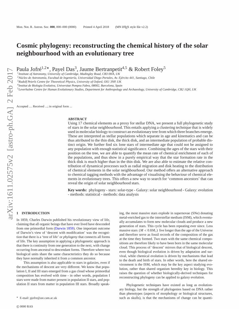
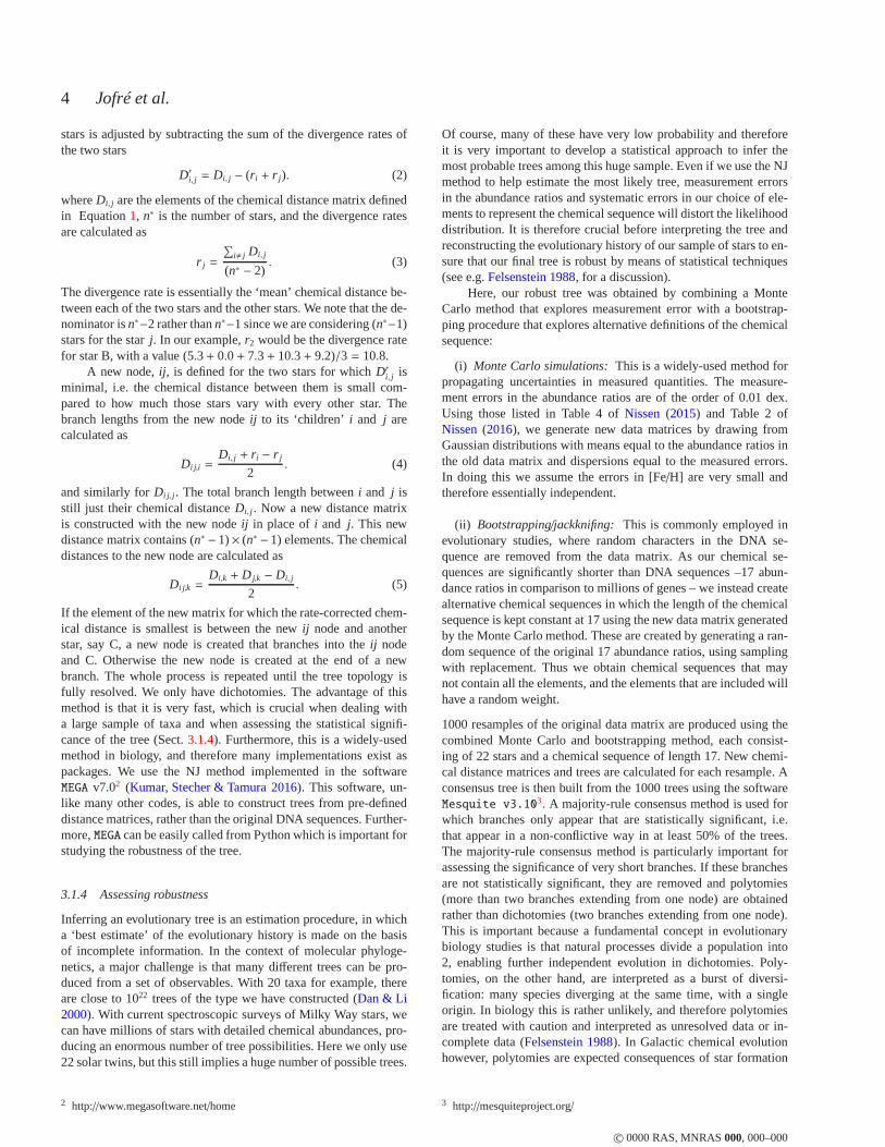
Figure1 presents our consensus tree. A tree constructed with the NJmethod is ‘unrooted’, and therefore even if clusters of stars appearto branch off initially from the same point, it does not signifiy thisis the beginning of the evolution of system. The radiation format(Fig. 1) for a phylogenetic tree is particularly suitable for visual-ising such trees as it emphasises that the groups and unclassifiedstars are separate from each other. The length of the branches are inchemical dex units with the scale indicated in the legend. They rep-resent the chemical distance between each star and the node fromwhich it emerged. The chemical distance between any two stars isdetermined by adding up the lengths of the branches between them.

The NJ method alone would only produce dichotomies, i.e.nodes split into two branches. However, the application of themajority-rule consensus method results in several polytomies,showing that some of the branches found in each of the 1000 treesin the resampling were not significant. Such polytomies could beexpected in chemical evolution when star formation bursts can re-sult in several stars driving different chemical enrichment paths, notjust two.

Even with the polytomies, three main stellar populations, i.e.groups of stars sharing a common ancestor, are identified. Thefirst one (red), includes the following stars: the Sun, HD 2071,HD 45184, HD 146233, HD 8406, HD 92719, HD 27063,HD 96116 and HD 134664. A second stellar population (blue)includes the stars: HD 210918, HD 45289 and HD 220507. Athird stellar population (orange) appears to be equally independentfrom the other two populations, and includes the stars HD 78429,HD 208704, HD 20782 and HD 38277. Finally, six stars (black)can not be assigned to any population with enough statisticalconfidence. These stars are HD 28471, HD 96423, HD 71334,HD 222582, HD 88084 and HD 183658. We comment here thatperhaps a different definition of chemical distance than the one em-ployed in Eq.1 might help to allocate some of these 6 stars into oneof the populations with better confidence but this is beyond the pur-pose of this work. Here we want to show that it is possible to applyphylogenetic analyses and tree thinking in the field of Galactic ar-chaeology. In this work we call these stars simply ‘undetermined’.

The branch lengths of the red stellar population are short, ofthe order of 0.1 dex, except for HD 96116, which has a branchlength of almost 0.4 dex. The branch lengths of the orange stellarpopulation are also of the order of 0.1 dex, reflecting that thesestars are very chemically similar to each other. The branch lengthsbetween the original polytomy and the first node in the blue stellarpopulation is significantly larger than the first nodes in thered andthe orange populations, but the branch lengths between nodes is ofthe same order of magnitude, with the exception of HD 220507,which has a branch length of 0.3 dex.

For guidance, the ages of the stars are indicated next to theirnames in Fig.1. The star furthest along the red right branch,HD 96116, is the youngest star of the sample (0.7 Gyr). It is moreseparate from the other stars in the red stellar population due toa larger chemical distance, and this is reflected in the ages of theother stars, which are clustered between 2.4 and 4.5 Gyr. The or-ange stellar population has stars that are chemically very similar

c© 0000 RAS, MNRAS000, 000–000

6 Jofré et al.

HD78429

HD220507

HD32877

HD20782

HD208704

7.8

8.1

8.3

9.8

9.49.1HD

45289

HD183658

HD88084

HD222582

HD71334

HD28471

HD96423

Sun

HD2071

HD45184

HD146233

HD8406

HD92719

HD96116

HD134664

HD27063

HD210918

7.4

5.2

5.9

7.0 8.8

7.3

7.3

4.5

3.5 2.7

4.0

4.1

2.5

2.8

2.4

0.7

9.56.9

7.9 3.0

Time (Gyr)

Figure 1. Unrooted phylogenetic tree. Three main branches are obtained and coloured with blue, red and orange. Stars that do not belong to any branch withstatistical significance are coloured with black. Branch lengths are in dex units, with the scale indicated at the bottomof the diagram.

0 20 40 60 80 100 120

|V| (km s−1)

0

20

40

60

80

100

120

(U2+W

2)1/2 (km s

−1)

1200 1400 1600 1800 2000 2200

|Lz| (kpc km s−1)

0

50

100

150

200

(Jr+Jz) kpc km s

−1

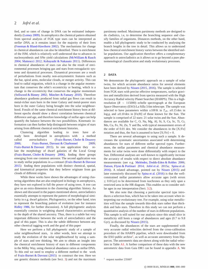
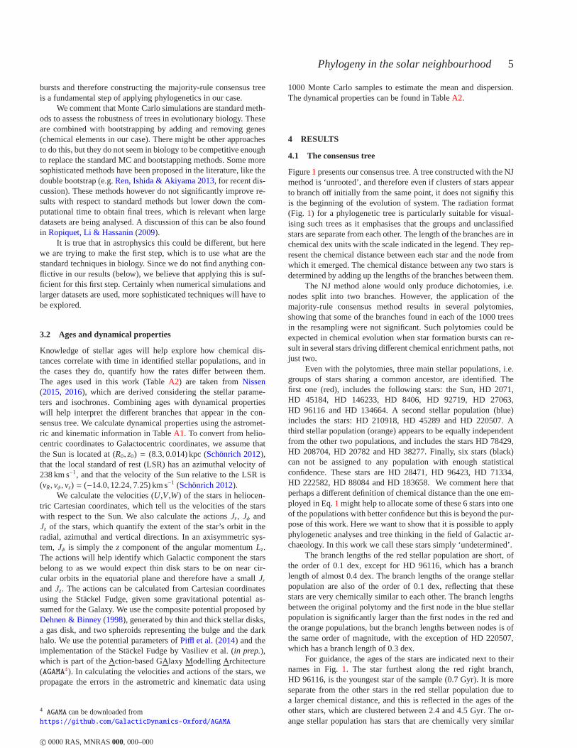
Figure 2. Toomre diagram (left) and the sum of the radial and vertical actions shown against thezcomponent of angular momentum (right). Stellar populationsare coloured according to the classification of the tree of Fig. 1.

to each other. Their ages are also in a restricted range of 0.9 Gyrbetween 7.4 and 8.3 Gyr.

The star furthest along the blue branch, HD 220507, is alsothe oldest star of the sample (9.8 Gyr). The other two stars in thisbranch have ages of 9.1 and 9.4 Gyr. The chemical distance be-tween the youngest and the oldest star is the largest in the tree at1.6 dex, and is obtained by adding the length of all the branchesthat separate the stars. The undetermined stars have ages between5.2 and 8.8 Gyr.

The mean age of all stars in a given population are indicated atthe bottom of Fig.1, following the colour coding of the branches.

We can see that the stellar populations have different ages, withtime increasing from left to right. The ages have told us thatthereis a very old stellar population (blue branch), a slightly youngerbut still old population (orange branch); stars of intermediate age(black branches), and a young stellar population (red branch). Weremark here that age was not used to build the tree.

Thus, the tree of Fig.1 adds a rough direction to the evolu-tionary processes, i.e. the older stars are found towards the left,while the younger stars are found towards the right. However, itis clear that in the region of overlap between the red, black,andblue branches, the stars belonging to separate stellar populations

c© 0000 RAS, MNRAS000, 000–000

Phylogeny in the solar neighbourhood 7

0 2 4 6 8 10τ (Gyr)

0.00

0.02

0.04

0.06

0.08

0.10

0.12

(Jr+Jz)/

|Lz|

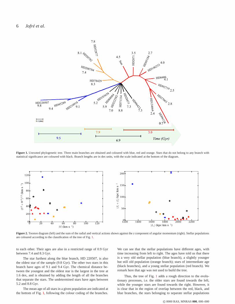
Figure 3.Eccentricity against age of the stars for the stellar populations andundetermined stars identified in Fig.1.

may have been produced from gas that was chemically enrichedatdifferent rates and exposed to dynamical processes such as heatingand radial migration. Therefore their location in this region is nolonger indicative of their age. We will come back to the importanceof dynamical processes in Sect.5.

4.2 Dynamics of the identified stellar populations

In order to study the nature of the identified stellar populationsmore clearly, we look at dynamical properties of the stars. The leftpanel of Fig.2 shows the classical Toomre diagram. They axis indi-cates the contribution to the star’s velocity in directionsperpendic-ular to that of Galactic rotation and thex axis indicates the contribu-tion to the star’s velocity along Galactic rotation, compared to thatof the Sun. Thin-disk stars should behave like the Sun, whilethickdisk and halo stars have velocities in random directions. Thereforethe stars in the red population that cluster around zero in both di-rections, and include the Sun, behave like thin-disk stars.The otherpopulations and undetermined stars cover a larger range in this plot,but in general tend to have higher values in both directions and aretherefore more likely to be thick-disk stars. They are unlikely to behalo stars because they are comparatively metal-rich.

The right panel in Fig.2 shows the ‘actions’ equivalent of theToomre diagram with the sum of the radial and vertical actionsshown against thez component of angular momentum,Lz. Thin-disk orbits are in the equatorial plane and should cluster inLz, aswe are restricted to the as solar neighbourhood. The red stars havea low total radial and vertical action and cluster inLz, and are there-fore probably thin-disk stars. The blue stars show a range oftotalradial and vertical actions and a larger spread in angular momen-tum and therefore could be thick-disk stars. The other starshave arange ofLz and low to intermediate total radial and vertical actions.

The stellar populations in terms of ages and dynamical prop-erties together are illustrated in Fig.3. The y axis combines theaxes of the left panel of Fig.2 into a dimensionless ratio of thesum of actions in the radial and vertical directions, divided by Lz.This dimensionless ratio is a measure of the eccentricity ofthe orbit(Sanders & Binney 2016) as it normalizes the radial and vertical ex-cursions of the star by the mean radius of the orbit. Thin-disk orbitsare circular and therefore should have a small eccentricitywhilethick-disk orbits should have a range of eccentricities. This is plot-ted against the age. The red stars are most likely to be thin-disk stars

as they have low eccentricities and have a spread in younger ages.The blue stars are most likely to be thick-disk stars as they are allold and have a range of eccentricities. The similarity between theorange stars is reflected clearly in their small range of ages. Theyhave a range in eccentricities that is intermediate betweenthe thinand thick disk.

The undetermined stars randomly span the ages between thethin and thick disks with a range of eccentricities intermediate be-tween the thin-disk and thick-disk stars. Some of these stars couldbelong to the older, flared part of the thin disk and the oldestmaybelong to the thick disk. The small number of data points meanshowever that if this were the case, the connection between thesestars and those in the thin and thick disk could not be recovered.

It should also be noted that the trend followed by the stars iscontinuous, restating the age-velocity dispersion relation (Wielen1977), i.e. older stars have a higher velocity dispersion and there-fore lie on more eccentric orbits. There is no evidence from thisplot that the data require separate components, and therefore a morecareful inspection of the abundance ratios is required (seeSect.5).

4.3 Evolution of stellar populations

To go further than simply identifying stellar populations,the phy-logenetic nature of the tree allows us to investigate the evolution ofchemical abundances within each stellar population. For example,any time a branch splits (i.e. there is a dichotomy or polytomy),we can interpret this as an instance at which the evolution ofthegas diverged. The stars arising from the split have formed from thesame or similar gas clouds. The further away a star in the poly-tomy is from the node the more evolved a gas cloud from which itoriginated.

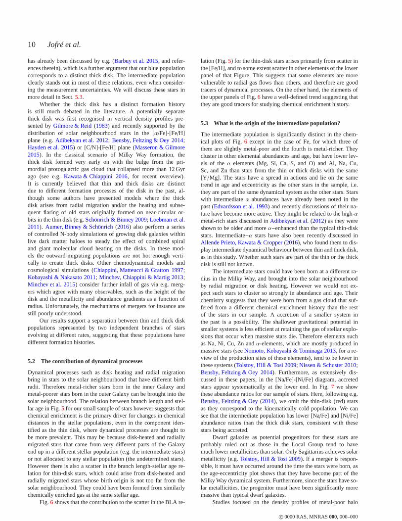
We study the chemical evolution within these differentGalactic components by exploiting the phylogenetic natureofthe tree. To do so, we redraw the tree of Fig.1 using a classicalformat in Fig.4, as this allows us to inspect the individual branchlengths in more detail. The Galactic components assigned toeach branch are indicated on the left and stellar ages on theright for guidance. Since we focus here only on stars that areassigned to a branch with enough statistical relevance, we considerthe blue, red, and orange branches independently, and calculatethe total branch length starting from the vertical line. This isdone by adding up the values indicated in each branch from thevertical line to each star. In Fig.5 we show the branch-lengthand age (BLA) relation, finding that branch length decreaseswith stellar age for the thick-disk (blue stars) but increases withstellar age for the thin-disk and intermediate stars (red and orangestars). This is simply a consequence of the location of the zeropoint in the tree. We would expect environmental processes anddynamical processes that have brought stars from a very differentpart of the Galaxy to branch out as separate stellar populations.Therefore within each branch we would expect a monotonictrend of stars increasing their elemental abundances with time.However, stars brought in from radii near to the solar neighbour-hood may be allocated to the same branch, adding scatter to thistrend. We can therefore make an estimate of the mean chemicalevolution rate and contributions from dynamical processesbycarrying out linear fits (dashed lines in Fig.5). Below we dis-cuss the chemical evolution history for the different groups of stars.

Thin disk:The BLA relation for the thin-disk stars is shown in redin Fig. 5. The stars are not consistent with being a single age, andtherefore the stars are likely to have formed in successive multi-

c© 0000 RAS, MNRAS000, 000–000

8 Jofré et al.

HD96423

HD28471

HD71334

HD222582

HD88084

HD183658

HD210918*

HD45289*

HD220507*

Thick Disk

HD78429

HD208704

HD20782

HD38277

Intermediate

Sun

HD2071

HD45184

HD146233

HD8406

HD92719

HD27063

HD96116

HD134664

Thin Disk

0.190

0.091

0.105

0.116

0.103

0.141

0.101

0.040

0.309

0.112

0.078

0.113

0.124

0.124

0.086

0.083

0.083

0.097

0.124

0.085

0.397

0.109

0.164

0.362

0.028

0.117

0.085

0.100

0.070

0.060

0.046

0.098

0.1 [dex]

7.3

7.3

8.8

Thick Disk

Thin Disk

Intermediate

5.9

7.0

5.2

9.4

9.1

9.8

7.4

8.3

8.1

7.8

3.5

4.5

2.7

4.1

4.0

2.5

0.7

2.8

2.4

Age

(Gyr)

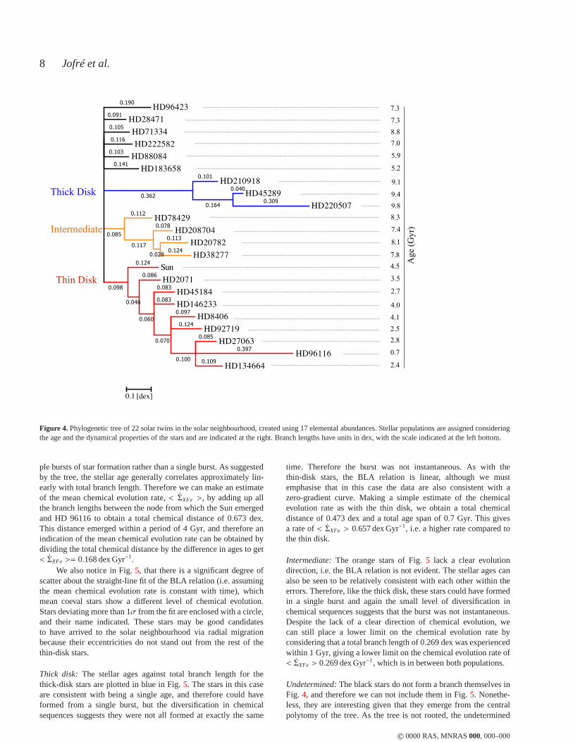
Figure 4. Phylogenetic tree of 22 solar twins in the solar neighbourhood, created using 17 elemental abundances. Stellar populations are assigned consideringthe age and the dynamical properties of the stars and are indicated at the right. Branch lengths have units in dex, with thescale indicated at the left bottom.

ple bursts of star formation rather than a single burst. As suggestedby the tree, the stellar age generally correlates approximately lin-early with total branch length. Therefore we can make an estimateof the mean chemical evolution rate,< ΣXFe >, by adding up allthe branch lengths between the node from which the Sun emergedand HD 96116 to obtain a total chemical distance of 0.673 dex.This distance emerged within a period of 4 Gyr, and thereforeanindication of the mean chemical evolution rate can be obtained bydividing the total chemical distance by the difference in ages to get< ΣXFe >= 0.168 dex Gyr−1.

We also notice in Fig.5, that there is a significant degree ofscatter about the straight-line fit of the BLA relation (i.e.assumingthe mean chemical evolution rate is constant with time), whichmean coeval stars show a different level of chemical evolution.Stars deviating more than 1σ from the fit are enclosed with a circle,and their name indicated. These stars may be good candidatesto have arrived to the solar neighbourhood via radial migrationbecause their eccentricities do not stand out from the rest of thethin-disk stars.

Thick disk: The stellar ages against total branch length for thethick-disk stars are plotted in blue in Fig.5. The stars in this caseare consistent with being a single age, and therefore could haveformed from a single burst, but the diversification in chemicalsequences suggests they were not all formed at exactly the same

time. Therefore the burst was not instantaneous. As with thethin-disk stars, the BLA relation is linear, although we mustemphasise that in this case the data are also consistent withazero-gradient curve. Making a simple estimate of the chemicalevolution rate as with the thin disk, we obtain a total chemicaldistance of 0.473 dex and a total age span of 0.7 Gyr. This givesa rate of< ΣXFe > 0.657 dex Gyr−1, i.e. a higher rate compared tothe thin disk.

Intermediate:The orange stars of Fig.5 lack a clear evolutiondirection, i.e. the BLA relation is not evident. The stellarages canalso be seen to be relatively consistent with each other within theerrors. Therefore, like the thick disk, these stars could have formedin a single burst and again the small level of diversificationinchemical sequences suggests that the burst was not instantaneous.Despite the lack of a clear direction of chemical evolution,wecan still place a lower limit on the chemical evolution rate byconsidering that a total branch length of 0.269 dex was experiencedwithin 1 Gyr, giving a lower limit on the chemical evolution rate of< ΣXFe > 0.269 dex Gyr−1, which is in between both populations.

Undetermined:The black stars do not form a branch themselves inFig. 4, and therefore we can not include them in Fig.5. Nonethe-less, they are interesting given that they emerge from the centralpolytomy of the tree. As the tree is not rooted, the undetermined

c© 0000 RAS, MNRAS000, 000–000

Phylogeny in the solar neighbourhood 9

−0.3 −0.2 −0.1 0.0 0.1 0.2[Y/Mg]

−0.05

0.00

0.05

0.10

0.15

[Mg/

Fe]

A

−0.3 −0.2 −0.1 0.0 0.1 0.2[Y/Mg]

−0.04

−0.02

0.00

0.02

0.04

0.06

0.08

[Si/F

e]

B

−0.3 −0.2 −0.1 0.0 0.1 0.2[Y/Mg]

−0.10

−0.05

0.00

0.05

0.10

0.15

0.20

[Al/F

e]

C

−0.3 −0.2 −0.1 0.0 0.1 0.2[Y/Mg]

−0.05

−0.00

0.05

0.10

0.15

[Sc/

Fe]

D

−0.3 −0.2 −0.1 0.0 0.1 0.2[Y/Mg]

−0.10

−0.05

0.00

0.05

0.10

0.15

[Zn/

Fe]

E

−0.3 −0.2 −0.1 0.0 0.1 0.2[Y/Mg]

−0.15

−0.10

−0.05

0.00

0.05

0.10

0.15

[Fe/

H]

F

−0.3 −0.2 −0.1 0.0 0.1 0.2[Y/Mg]

0.00

0.01

0.02

0.03

0.04

0.05

0.06

[Ca/

Fe]

G

−0.3 −0.2 −0.1 0.0 0.1 0.2[Y/Mg]

−0.10

−0.05

−0.00

0.05

[Na/

Fe]

H

−0.3 −0.2 −0.1 0.0 0.1 0.2[Y/Mg]

−0.08

−0.06

−0.04

−0.02

0.00

0.02

[Mn/

Fe]

I

−0.3 −0.2 −0.1 0.0 0.1 0.2[Y/Mg]

−0.06

−0.04

−0.02

0.00

0.02

0.04

[Ni/F

e]

J

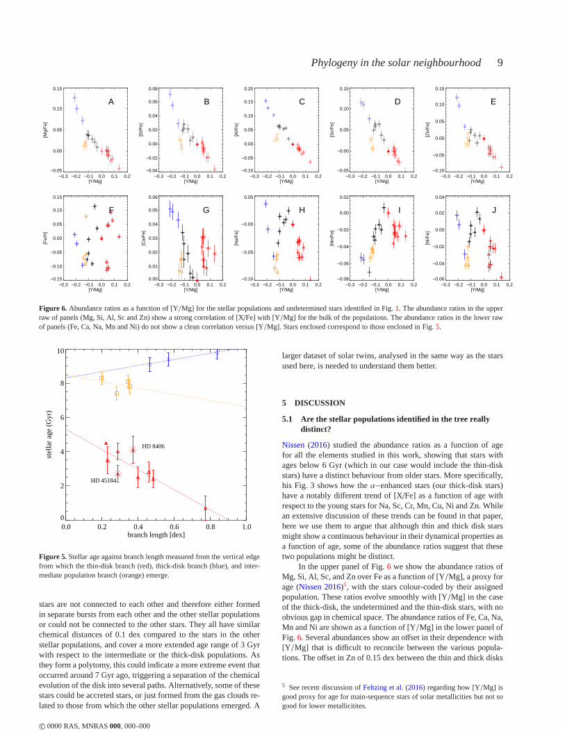
Figure 6. Abundance ratios as a function of [Y/Mg] for the stellar populations and undetermined stars identified in Fig.1. The abundance ratios in the upperraw of panels (Mg, Si, Al, Sc and Zn) show a strong correlationof [X /Fe] with [Y/Mg] for the bulk of the populations. The abundance ratios in the lower rawof panels (Fe, Ca, Na, Mn and Ni) do not show a clean correlation versus [Y/Mg]. Stars enclosed correspond to those enclosed in Fig.5.

0.0 0.2 0.4 0.6 0.8 1.0branch length [dex]

0

2

4

6

8

10

stel

lar

age

(Gyr

)

HD 8406

HD 45184

Figure 5. Stellar age against branch length measured from the vertical edgefrom which the thin-disk branch (red), thick-disk branch (blue), and inter-mediate population branch (orange) emerge.

stars are not connected to each other and therefore either formedin separate bursts from each other and the other stellar populationsor could not be connected to the other stars. They all have similarchemical distances of 0.1 dex compared to the stars in the otherstellar populations, and cover a more extended age range of 3Gyrwith respect to the intermediate or the thick-disk populations. Asthey form a polytomy, this could indicate a more extreme event thatoccurred around 7 Gyr ago, triggering a separation of the chemicalevolution of the disk into several paths. Alternatively, some of thesestars could be accreted stars, or just formed from the gas clouds re-lated to those from which the other stellar populations emerged. A

larger dataset of solar twins, analysed in the same way as thestarsused here, is needed to understand them better.

5 DISCUSSION

5.1 Are the stellar populations identified in the tree reallydistinct?

Nissen(2016) studied the abundance ratios as a function of agefor all the elements studied in this work, showing that starswithages below 6 Gyr (which in our case would include the thin-diskstars) have a distinct behaviour from older stars. More specifically,his Fig. 3 shows how theα−enhanced stars (our thick-disk stars)have a notably different trend of [X/Fe] as a function of age withrespect to the young stars for Na, Sc, Cr, Mn, Cu, Ni and Zn. Whilean extensive discussion of these trends can be found in that paper,here we use them to argue that although thin and thick disk starsmight show a continuous behaviour in their dynamical properties asa function of age, some of the abundance ratios suggest that thesetwo populations might be distinct.

In the upper panel of Fig.6 we show the abundance ratios ofMg, Si, Al, Sc, and Zn over Fe as a function of [Y/Mg], a proxy forage (Nissen 2016)5, with the stars colour-coded by their assignedpopulation. These ratios evolve smoothly with [Y/Mg] in the caseof the thick-disk, the undetermined and the thin-disk stars, with noobvious gap in chemical space. The abundance ratios of Fe, Ca, Na,Mn and Ni are shown as a function of [Y/Mg] in the lower panel ofFig. 6. Several abundances show an offset in their dependence with[Y/Mg] that is difficult to reconcile between the various popula-tions. The offset in Zn of 0.15 dex between the thin and thick disks

5 See recent discussion ofFeltzing et al.(2016) regarding how [Y/Mg] isgood proxy for age for main-sequence stars of solar metallicities but not sogood for lower metallicitites.

c© 0000 RAS, MNRAS000, 000–000

10 Jofré et al.

has already been discussed by e.g. (Barbuy et al. 2015, and refer-ences therein), which is a further argument that our blue populationcorresponds to a distinct thick disk. The intermediate populationclearly stands out in most of these relations, even when consider-ing the measurement uncertainties. We will discuss these stars inmore detail in Sect.5.3.

Whether the thick disk has a distinct formation historyis still much debated in the literature. A potentially separatethick disk was first recognised in vertical density profiles pre-sented byGilmore & Reid (1983) and recently supported by thedistribution of solar neighbourhood stars in the [α/Fe]-[Fe/H]plane (e.g.Adibekyan et al. 2012; Bensby, Feltzing & Oey 2014;Hayden et al. 2015) or [C/N]-[Fe/H] plane (Masseron & Gilmore2015). In the classical scenario of Milky Way formation, thethick disk formed very early on with the bulge from the pri-mordial protogalactic gas cloud that collapsed more than 12Gyrago (see e.g.Kawata & Chiappini 2016, for recent overview).It is currently believed that thin and thick disks are distinctdue to different formation processes of the disk in the past, al-though some authors have presented models where the thickdisk arises from radial migration and/or the heating and subse-quent flaring of old stars originally formed on near-circular or-bits in the thin disk (e.g.Schönrich & Binney 2009; Loebman et al.2011). Aumer, Binney & Schönrich(2016) also perform a seriesof controlled N-body simulations of growing disk galaxies withinlive dark matter haloes to steady the effect of combined spiraland giant molecular cloud heating on the disks. In these mod-els the outward-migrating populations are not hot enough verti-cally to create thick disks. Other chemodynamical models andcosmological simulations (Chiappini, Matteucci & Gratton 1997;Kobayashi & Nakasato 2011; Minchev, Chiappini & Martig 2013;Minchev et al. 2015) consider further infall of gas via e.g. merg-ers which agree with many observables, such as the height of thedisk and the metallicity and abundance gradients as a function ofradius. Unfortunately, the mechanisms of mergers for instance arestill poorly understood.

Our results support a separation between thin and thick diskpopulations represented by two independent branches of starsevolving at different rates, suggesting that these populations havedifferent formation histories.

5.2 The contribution of dynamical processes

Dynamical processes such as disk heating and radial migrationbring in stars to the solar neighbourhood that have different birthradii. Therefore metal-richer stars born in the inner Galaxy andmetal-poorer stars born in the outer Galaxy can be brought into thesolar neighbourhood. The relation between branch length and stel-lar age in Fig.5 for our small sample of stars however suggests thatchemical enrichment is the primary driver for changes in chemicaldistances in the stellar populations, even in the componentiden-tified as the thin disk, where dynamical processes are thought tobe more prevalent. This may be because disk-heated and radiallymigrated stars that came from very different parts of the Galaxyend up in a different stellar population (e.g. the intermediate stars)or not allocated to any stellar population (the undetermined stars).However there is also a scatter in the branch length-stellarage re-lation for thin-disk stars, which could arise from disk-heated andradially migrated stars whose birth origin is not too far from thesolar neighbourhood. They could have been formed from similarlychemically enriched gas at the same stellar age.

Fig. 6 shows that the contribution to the scatter in the BLA re-

lation (Fig.5) for the thin-disk stars arises primarily from scatter inthe [Fe/H], and to some extent scatter in other elements of the lowerpanel of that Figure. This suggests that some elements are morevulnerable to radial gas flows than others, and therefore aregoodtracers of dynamical processes. On the other hand, the elements ofthe upper panels of Fig.6 have a well-defined trend suggesting thatthey are good tracers for studying chemical enrichment history.

5.3 What is the origin of the intermediate population?

The intermediate population is significantly distinct in the chem-ical plots of Fig.6 except in the case of Fe, for which three ofthem are slightly metal-poor and the fourth is metal-richer. Theycluster in other elemental abundances and age, but have lower lev-els of theα elements (Mg, Si, Ca, S, and O) and Al, Na, Cu,Sc, and Zn than stars from the thin or thick disks with the same[Y/Mg]. The stars have a spread in actions and lie on the sametrend in age and eccentricity as the other stars in the sample, i.e.they are part of the same dynamical system as the other stars.Starswith intermediateα abundances have already been noted in thepast (Edvardsson et al. 1993) and recently discussions of their na-ture have become more active. They might be related to the high-αmetal-rich stars discussed inAdibekyan et al.(2012) as they wereshown to be older and moreα−enhanced than the typical thin-diskstars. Intermediate−α stars have also been recently discussed inAllende Prieto, Kawata & Cropper(2016), who found them to dis-play intermediate dynamical behaviour between thin and thick disk,as in this study. Whether such stars are part of the thin or thethickdisk is still not known.

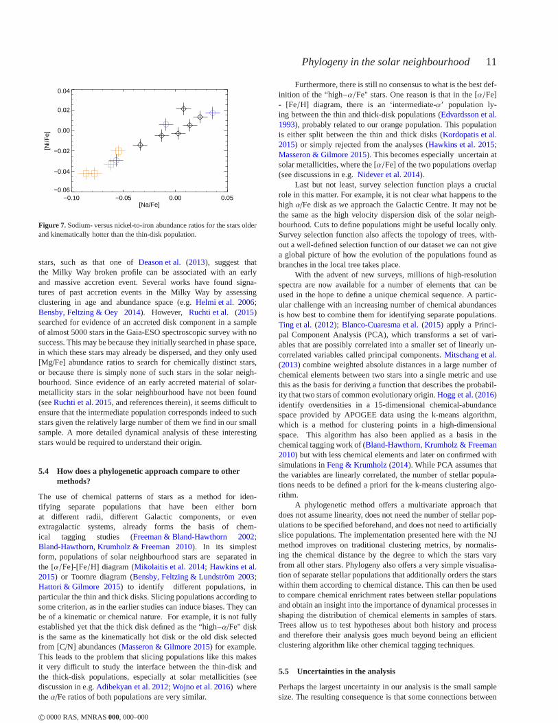
The intermediate stars could have been born at a different ra-dius in the Milky Way, and brought into the solar neighbourhoodby radial migration or disk heating. However we would not ex-pect such stars to cluster so strongly in abundance and age. Theirchemistry suggests that they were born from a gas cloud that suf-fered from a different chemical enrichment history than the restof the stars in our sample. A accretion of a smaller system inthe past is a possibility. The shallower gravitational potential insmaller systems is less efficient at retaining the gas of stellar explo-sions that occur when massive stars die. Therefore elementssuchas Na, Ni, Cu, Zn andα-elements, which are mostly produced inmassive stars (seeNomoto, Kobayashi & Tominaga 2013, for a re-view of the production sites of these elements), tend to be lower inthese systems (Tolstoy, Hill & Tosi 2009; Nissen & Schuster 2010;Bensby, Feltzing & Oey 2014). Furthermore, as extensively dis-cussed in these papers, in the [Na/Fe]-[Ni/Fe] diagram, accretedstars appear systematically at the lower end. In Fig.7 we showthese abundance ratios for our sample of stars. Here, following e.g.Bensby, Feltzing & Oey(2014), we omit the thin-disk (red) starsas they correspond to the kinematically cold population. Wecansee that the intermediate population has lower [Na/Fe] and [Ni/Fe]abundance ratios than the thick disk stars, consistent withthesestars being accreted.

Dwarf galaxies as potential progenitors for these stars areprobably ruled out as those in the Local Group tend to havemuch lower metallicities than solar. Only Sagittarius achieves solarmetallicity (e.g.Tolstoy, Hill & Tosi 2009). If a merger is respon-sible, it must have occurred around the time the stars were born, asthe age-eccentricity plot shows that they have become part of theMilky Way dynamical system. Furthermore, since the stars have so-lar metallicities, the progenitor must have been significantly moremassive than typical dwarf galaxies.

Studies focused on the density profiles of metal-poor halo

c© 0000 RAS, MNRAS000, 000–000

Phylogeny in the solar neighbourhood 11

−0.10 −0.05 0.00 0.05[Na/Fe]

−0.06

−0.04

−0.02

0.00

0.02

0.04

[Ni/F

e]

Figure 7.Sodium- versus nickel-to-iron abundance ratios for the stars olderand kinematically hotter than the thin-disk population.

stars, such as that one ofDeason et al.(2013), suggest thatthe Milky Way broken profile can be associated with an earlyand massive accretion event. Several works have found signa-tures of past accretion events in the Milky Way by assessingclustering in age and abundance space (e.g.Helmi et al. 2006;Bensby, Feltzing & Oey 2014). However, Ruchti et al. (2015)searched for evidence of an accreted disk component in a sampleof almost 5000 stars in the Gaia-ESO spectroscopic survey with nosuccess. This may be because they initially searched in phase space,in which these stars may already be dispersed, and they only used[Mg/Fe] abundance ratios to search for chemically distinct stars,or because there is simply none of such stars in the solar neigh-bourhood. Since evidence of an early accreted material of solar-metallicity stars in the solar neighbourhood have not been found(seeRuchti et al. 2015, and references therein), it seems difficult toensure that the intermediate population corresponds indeed to suchstars given the relatively large number of them we find in our smallsample. A more detailed dynamical analysis of these interestingstars would be required to understand their origin.

5.4 How does a phylogenetic approach compare to othermethods?

The use of chemical patterns of stars as a method for iden-tifying separate populations that have been either bornat different radii, different Galactic components, or evenextragalactic systems, already forms the basis of chem-ical tagging studies (Freeman & Bland-Hawthorn 2002;Bland-Hawthorn, Krumholz & Freeman 2010). In its simplestform, populations of solar neighbourhood stars are separated inthe [α/Fe]-[Fe/H] diagram (Mikolaitis et al. 2014; Hawkins et al.2015) or Toomre diagram (Bensby, Feltzing & Lundström 2003;Hattori & Gilmore 2015) to identify different populations, inparticular the thin and thick disks. Slicing populations according tosome criterion, as in the earlier studies can induce biases.They canbe of a kinematic or chemical nature. For example, it is not fullyestablished yet that the thick disk defined as the “high−α/Fe" diskis the same as the kinematically hot disk or the old disk selectedfrom [C/N] abundances (Masseron & Gilmore 2015) for example.This leads to the problem that slicing populations like thismakesit very difficult to study the interface between the thin-disk andthe thick-disk populations, especially at solar metallicities (seediscussion in e.g.Adibekyan et al. 2012; Wojno et al. 2016) wheretheα/Fe ratios of both populations are very similar.

Furthermore, there is still no consensus to what is the best def-inition of the “high−α/Fe" stars. One reason is that in the [α/Fe]- [Fe/H] diagram, there is an ‘intermediate-α’ population ly-ing between the thin and thick-disk populations (Edvardsson et al.1993), probably related to our orange population. This populationis either split between the thin and thick disks (Kordopatis et al.2015) or simply rejected from the analyses (Hawkins et al. 2015;Masseron & Gilmore 2015). This becomes especially uncertain atsolar metallicities, where the [α/Fe] of the two populations overlap(see discussions in e.g.Nidever et al. 2014).

Last but not least, survey selection function plays a crucialrole in this matter. For example, it is not clear what happensto thehigh α/Fe disk as we approach the Galactic Centre. It may not bethe same as the high velocity dispersion disk of the solar neigh-bourhood. Cuts to define populations might be useful locallyonly.Survey selection function also affects the topology of trees, with-out a well-defined selection function of our dataset we can not givea global picture of how the evolution of the populations found asbranches in the local tree takes place.

With the advent of new surveys, millions of high-resolutionspectra are now available for a number of elements that can beused in the hope to define a unique chemical sequence. A partic-ular challenge with an increasing number of chemical abundancesis how best to combine them for identifying separate populations.Ting et al. (2012); Blanco-Cuaresma et al.(2015) apply a Princi-pal Component Analysis (PCA), which transforms a set of vari-ables that are possibly correlated into a smaller set of linearly un-correlated variables called principal components.Mitschang et al.(2013) combine weighted absolute distances in a large number ofchemical elements between two stars into a single metric andusethis as the basis for deriving a function that describes the probabil-ity that two stars of common evolutionary origin.Hogg et al.(2016)identify overdensities in a 15-dimensional chemical-abundancespace provided by APOGEE data using the k-means algorithm,which is a method for clustering points in a high-dimensionalspace. This algorithm has also been applied as a basis in thechemical tagging work of (Bland-Hawthorn, Krumholz & Freeman2010) but with less chemical elements and later on confirmed withsimulations inFeng & Krumholz(2014). While PCA assumes thatthe variables are linearly correlated, the number of stellar popula-tions needs to be defined a priori for the k-means clustering algo-rithm.

A phylogenetic method offers a multivariate approach thatdoes not assume linearity, does not need the number of stellar pop-ulations to be specified beforehand, and does not need to artificiallyslice populations. The implementation presented here withthe NJmethod improves on traditional clustering metrics, by normalis-ing the chemical distance by the degree to which the stars varyfrom all other stars. Phylogeny also offers a very simple visualisa-tion of separate stellar populations that additionally orders the starswithin them according to chemical distance. This can then beusedto compare chemical enrichment rates between stellar populationsand obtain an insight into the importance of dynamical processes inshaping the distribution of chemical elements in samples ofstars.Trees allow us to test hypotheses about both history and processand therefore their analysis goes much beyond being an efficientclustering algorithm like other chemical tagging techniques.

5.5 Uncertainties in the analysis

Perhaps the largest uncertainty in our analysis is the smallsamplesize. The resulting consequence is that some connections between

c© 0000 RAS, MNRAS000, 000–000

12 Jofré et al.

stars may have been missed, thus not allowing a full recoveryof thechemical enrichment history.

In addition, we have only explored a single method for con-structing the phylogenetic tree (NJ, see Sect.3). Although we haveassessed the robustness of applying this particular method, thereare several other methods in the literature that may result in dif-ferent groupings and branch lengths, and therefore a different phy-logeny. There are other ways of constructing the distance matrixand translating this into a tree. There are also methods thatdo notrely on constructing a distance matrix. Particular types ofevolu-tionary events can be penalized in the construction of the tree cost,and then an attempt is made to locate the tree with the smallest to-tal cost. The maximum likelihood and Bayesian approaches assignprobabilities to particular possible phylogenetic trees.The methodis broadly similar to the maximum-parsimony method, but allowsboth varying rates of evolution as well as different probabilities ofparticular events. While this method is computationally expensiveand therefore not easy to use for large datasets, it remains to betested in future applications within Galactic archaeology.

As with chemical tagging studies, the method presented hererelies on the uniqueness of stellar DNA. We ascertain that aslongas enough elements are used in the analysis, this should be the case(Hogg et al. 2016). We need to be aware however that our sam-ple needs to be chosen such that the chemical distances are re-flecting differences in chemical evolution and not systematic differ-ences due to internal processes happening in stars, such as atomicdiffusion (e.g.Gruyters et al. 2013), pollution due to binary com-panions (McClure, Fletcher & Nemec 1980) or even enrichmentdue to accretion of gas from the ISM (Shen et al. 2016). There-fore it is important to have a sample of stars with the same spectralclass (see e.g. extensive discussion inBlanco-Cuaresma et al. 2015;Jofré et al. 2015a; Jofré et al. 2016).

6 SUMMARY AND CONCLUSIONS

We demonstrate the potential for the use of a phylogenetic methodin visualising and analysing the chemical evolution of solar neigh-bourhood stars, using abundances of 17 chemical elements for the22 solar twins ofNissen(2015, 2016) as a proxy for DNA. Thechemical abundances were used to create a matrix of the chemi-cal distances between pair of stars. This matrix was input into asoftware developed for molecular biology to create a phylogenetictree. Despite the small size of the sample, we believe the methodsuccessfully recovered stellar populations with distinctchemicalenrichment histories and produced a succinct visualisation of thestars in a multi-dimensional chemical space.

A comparison of the order of the stars along tree brancheswith stellar ages confirmed that the order generally traces the di-rection of chemical enrichment, thus allowing an estimate of themean chemical enrichment rate to be made. Chemical enrichmenthas a mean rate of< ΣXFe >= 0.168 dex Gyr−1 in the thin disk,< ΣXFe >= 0.657 dex Gyr−1 in the thick disk, and< ΣXFe >=

0.269 dex Gyr−1 in the intermediate population of stars. Our analy-sis thus confirms, in a purely empirical way, that the star formationrate in the thick disk is much faster than in the thin disk.

In addition to confirming a likely separate chemical enrich-ment history in the thin disk compared to the thick disk, we alsofind a separate population, intermediate in age and eccentricitiesbut distinct and clustered in several abundance ratios. Dueto itsold age and low abundances ofα− and other iron-peak elementswith respect to coeval stars in the thin and thick-disk populations,

we surmise that these stars could have arrived via a major mergerat the early stages of the Milky Way formation. We however couldnot rule out the possibility that these stars might be the youngesttail of the thick disk or the oldest tail of the thin disk, as they be-longed to similar trends in some abundance ratios and kinematicalproperties. The fact they emerge as an independent branch inourtree could be either due to a truly different nature or due to selec-tion effects. We conclude that a more detailed dynamical study ofsuch stars and a larger sample of old solar-metallicity stars is neces-sary. Future work will also benefit greatly from tests on simulatedstars in the solar neighbourhood in order to better understand howradially migrated and disk heated stars appear in the phylogenetictree.

In biology it is commonly said that to study evolution, oneessentially analyses trees. Galactic archaeology should be no dif-ferent, especially now, during its golden ages. Thanks to Gaia andits complementary spectroscopic and asteroseismic surveys, we arequickly getting chemical abundances of millions of stars which canbe complemented with accurate astrometry and ages. These richdatasets are on the verge of putting us closer to finding the one treethat connects all stars in the Milky Way.

Acknowledgments

We are deeply grateful to K.M. Reinhart, G. Weiss-Sussex andB.Burgwinkle for organising the research event in King’s CollegeCambridge that inspired this work. We also thank P. E. Nissenfor useful comments about this manuscript. P.J. acknowledges C.Worley, T. Masseron, T. Mädler and G. Gilmore and P.D. thanksD. Labonte, J. Binney and the Oxford Galactic Dynamics groupfor discussions on the topic. We acknowledge the positive feed-back from the referee report. The research leading to these resultshas received funding from the European Research Council underthe European Union’s Seventh Framework Programme (FP7/2007-2013)/ERC grant agreement no.s 320360 and 321067, as well asKing’s College Cambridge CRA programme.

REFERENCES

Adibekyan V. Z., Sousa S. G., Santos N. C., Delgado Mena E.,González Hernández J. I., Israelian G., Mayor M., KhachatryanG., 2012, A&A, 545, A32

Allende Prieto C., Kawata D., Cropper M., 2016, ArXiv e-printsAumer M., Binney J., Schönrich R., 2016, MNRAS, 459, 3326Barbuy B. et al., 2015, A&A, 580, A40Bensby T., Feltzing S., Lundström I., 2003, A&A, 410, 527Bensby T., Feltzing S., Oey M. S., 2014, A&A, 562, A71Blanco-Cuaresma S. et al., 2015, A&A, 577, A47Bland-Hawthorn J., Krumholz M. R., Freeman K., 2010, ApJ,713, 166

Chiappini C., Matteucci F., Gratton R., 1997, ApJ, 477, 765Dan G., Li W.-H., 2000, Fundamentals of molecular evolutionDarwin C., 1859, Ed. Joseph Carroll. Toronto: Broadview, 2003edition

Datson J., Flynn C., Portinari L., 2014, MNRAS, 439, 1028De Silva G. M. et al., 2015, MNRAS, 449, 2604Deason A. J., Belokurov V., Evans N. W., Johnston K. V., 2013,ApJ, 763, 113

Dehnen W., Binney J., 1998, MNRAS, 294, 429Edvardsson B., Andersen J., Gustafsson B., Lambert D. L., NissenP. E., Tomkin J., 1993, A&AS, 102, 603

c© 0000 RAS, MNRAS000, 000–000

Phylogeny in the solar neighbourhood 13

Felsenstein J., 1982, The Quarterly Review of Biology, 57, 379Felsenstein J., 1988, Annual review of genetics, 22, 521Feltzing S., Howes L. M., McMillan P. J., Stonkute E., 2016,ArXiv e-prints

Feng Y., Krumholz M. R., 2014, Nature, 513, 523Fraix-Burnet D., Choler P., Douzery E. J. P., 2006, A&A, 455,845Fraix-Burnet D., Davoust E., 2015, MNRAS, 450, 3431Fraix-Burnet D., Davoust E., Charbonnel C., 2009, MNRAS, 398,1706

Freeman K., Bland-Hawthorn J., 2002, ARA&A, 40, 487Gaia Collaboration, Brown A. G. A., Vallenari A., Prusti T.,deBruijne J., Mignard F., Drimmel R., co-authors ., 2016, ArXive-prints

Gilmore G., Reid N., 1983, MNRAS, 202, 1025Gruyters P., Korn A. J., Richard O., Grundahl F., Collet R.,Mashonkina L. I., Osorio Y., Barklem P. S., 2013, A&A, 555,A31

Hattori K., Gilmore G., 2015, MNRAS, 454, 649Hawkins K., Jofré P., Masseron T., Gilmore G., 2015, MNRAS,453, 758

Hayden M. R. et al., 2015, ApJ, 808, 132Helmi A., Navarro J. F., Nordström B., Holmberg J., Abadi M. G.,Steinmetz M., 2006, MNRAS, 365, 1309

Hogg D. W. et al., 2016, ArXiv e-printsJofré P. et al., 2015a, A&A, 582, A81Jofré P. et al., 2016, ArXiv e-printsJofré P., Mädler T., Gilmore G., Casey A. R., Soubiran C., WorleyC., 2015b, MNRAS, 453, 1428

Kawata D., Chiappini C., 2016, ArXiv e-printsKobayashi C., Nakasato N., 2011, ApJ, 729, 16Kordopatis G. et al., 2015, A&A, 582, A122Kumar S., Stecher G., Tamura K., 2016, Molecular biology andevolution, msw054

Lemey P., 2009, The phylogenetic handbook: a practical approachto phylogenetic analysis and hypothesis testing. Cambridge Uni-versity Press

Loebman S. R., Roškar R., Debattista V. P., Ivezic Ž., Quinn T. R.,Wadsley J., 2011, ApJ, 737, 8

Masseron T., Gilmore G., 2015, MNRAS, 453, 1855Matteucci F., 2012, Chemical Evolution of GalaxiesMcClure R. D., Fletcher J. M., Nemec J. M., 1980, ApJLett, 238,L35

McWilliam A., Rauch M., 2004, Origin and Evolution of the Ele-ments

Meléndez J., Dodds-Eden K., Robles J. A., 2006, ApJLett, 641,L133

Mikolaitis Š. et al., 2014, A&A, 572, A33Minchev I., Chiappini C., Martig M., 2013, A&A, 558, A9Minchev I., Famaey B., 2010, ApJ, 722, 112Minchev I., Martig M., Streich D., Scannapieco C., de Jong R.S.,Steinmetz M., 2015, ApJLett, 804, L9

Mitschang A. W., De Silva G., Sharma S., Zucker D. B., 2013,MNRAS, 428, 2321

Nidever D. L. et al., 2014, ApJ, 796, 38Nissen P. E., 2015, A&A, 579, A52Nissen P. E., 2016, A&A, 593, A65Nissen P. E., Schuster W. J., 2010, A&A, 511, L10Nomoto K., Kobayashi C., Tominaga N., 2013, ARA&A, 51, 457Piffl T. et al., 2014, MNRAS, 445, 3133Ren A., Ishida T., Akiyama Y., 2013, Molecular phylogenetics andevolution, 67, 429

Ridley M., 1986

0.8

0.9

1.0

1.1

1.2Parallax

HD

2071

HD

8406

HD

2706

3

HD

3827

7

HD

4518

4

HD

7842

9

HD

8808

4

HD

9611

6

HD

9642

3

HD

1346

64

HD

2087

04

HD

2205

07

HD

2225

82

0.8

0.9

1.0

1.1

1.2

1.3

1.4Proper motion (RA)

0.8

0.9

1.0

1.1

1.2Proper motion (DEC)

Hip

parc

os/G

aia

1.0

1.5

2.0

2.5

3.0

3.5

4.0Parallax error

HD

2071

HD

8406

HD

2706

3

HD

3827

7

HD

4518

4

HD

7842

9

HD

8808

4

HD

9611

6

HD

9642

3

HD

1346

64

HD

2087

04

HD

2205

07

HD

2225

82

5.0

10.0

15.0

20.0Proper motion error (RA)

5.0

10.0

15.0

20.0Proper motion error (DEC)

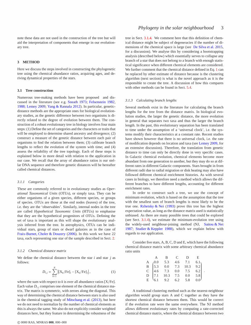
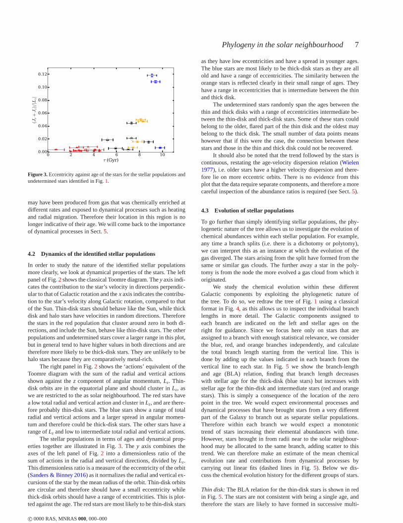
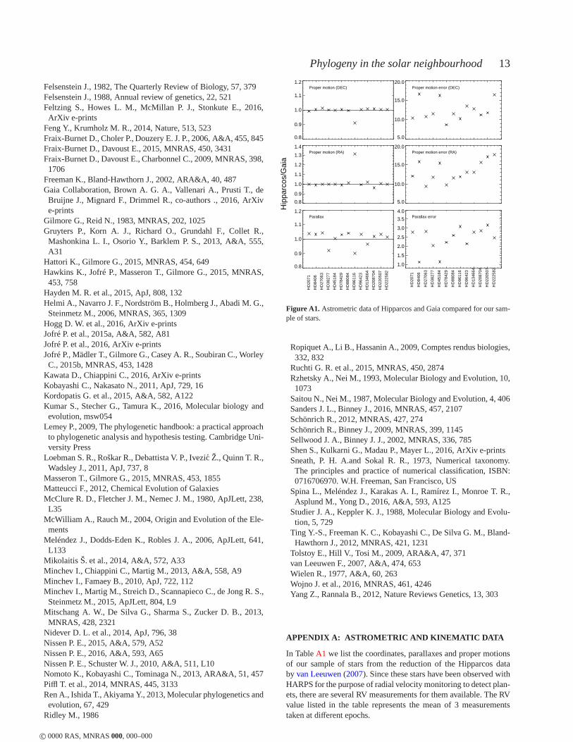
Figure A1. Astrometric data of Hipparcos and Gaia compared for our sam-ple of stars.

Ropiquet A., Li B., Hassanin A., 2009, Comptes rendus biologies,332, 832

Ruchti G. R. et al., 2015, MNRAS, 450, 2874Rzhetsky A., Nei M., 1993, Molecular Biology and Evolution,10,1073

Saitou N., Nei M., 1987, Molecular Biology and Evolution, 4,406Sanders J. L., Binney J., 2016, MNRAS, 457, 2107Schönrich R., 2012, MNRAS, 427, 274Schönrich R., Binney J., 2009, MNRAS, 399, 1145Sellwood J. A., Binney J. J., 2002, MNRAS, 336, 785Shen S., Kulkarni G., Madau P., Mayer L., 2016, ArXiv e-printsSneath, P. H. A.and Sokal R. R., 1973, Numerical taxonomy.The principles and practice of numerical classification, ISBN:0716706970. W.H. Freeman, San Francisco, US

Spina L., Meléndez J., Karakas A. I., Ramírez I., Monroe T. R.,Asplund M., Yong D., 2016, A&A, 593, A125

Studier J. A., Keppler K. J., 1988, Molecular Biology and Evolu-tion, 5, 729

Ting Y.-S., Freeman K. C., Kobayashi C., De Silva G. M., Bland-Hawthorn J., 2012, MNRAS, 421, 1231

Tolstoy E., Hill V., Tosi M., 2009, ARA&A, 47, 371van Leeuwen F., 2007, A&A, 474, 653Wielen R., 1977, A&A, 60, 263Wojno J. et al., 2016, MNRAS, 461, 4246Yang Z., Rannala B., 2012, Nature Reviews Genetics, 13, 303

APPENDIX A: ASTROMETRIC AND KINEMATIC DATA

In TableA1 we list the coordinates, parallaxes and proper motionsof our sample of stars from the reduction of the Hipparcos databy van Leeuwen(2007). Since these stars have been observed withHARPS for the purpose of radial velocity monitoring to detect plan-ets, there are several RV measurements for them available. The RVvalue listed in the table represents the mean of 3 measurementstaken at different epochs.

c© 0000 RAS, MNRAS000, 000–000

14 Jofré et al.

Star RA DEC σ V pm(RA) pm(DEC) RV[degrees] [degrees] [mas] [mas] [mag] [mas/yr] [mas/yr] [km/s]

HD2071 0.1077987647 -0.9421973172 36.72 0.64 7.27 210.72 -27.9 6.6823HD8406 0.3622254703 -0.2877530204 27.38 0.79 7.92 -136.95-176.35 -7.6766HD20782 0.8729078992 -0.5035957911 28.15 0.62 7.36 349.33-65.92 39.9666HD27063 1.1192125265 -0.0099900057 24.09 0.62 8.07 -61.2 -174.37 -9.5868HD28471 1.1569520864 -1.1184218496 23.48 0.52 7.89 -61.21321.65 54.8322HD38277 1.5022599908 -0.1748188646 24.42 0.59 7.11 65.86 -143.64 32.7339HD45184 1.6787150866 -0.5023025992 45.7 0.4 6.37 -164.99 -121.77 -3.7577HD45289 1.6772913373 -0.7478632512 35.81 0.32 6.67 -77.14777.98 56.4638HD71334 2.207072235 -0.5223749846 26.64 0.78 7.81 139.04 -292.03 17.3836HD78429 2.3851954548 -0.7590858065 26.83 0.51 7.31 48.18 179.49 65.1012HD88084 2.6578675783 -0.2704215986 29.01 0.65 7.52 -93.59-196.69 -23.5602HD92719 2.8022119328 -0.2406336934 41.97 0.47 6.79 235.35-172.56 -17.8906HD96116 2.8982366461 -1.0081901354 16.96 0.74 8.65 31.49 -35.4 31.3132HD96423 2.9074038637 -0.7744568097 31.87 0.6 7.23 87.3 -86.9 54.8541HD134664 3.9800988033 -0.5390630337 23.36 0.75 7.76 99.89-105.82 7.6595HD146233 4.2569404686 -0.1460532782 71.94 0.37 5.49 230.77 -495.53 11.8365HD183658 5.1089279481 -0.113692144 31.93 0.6 7.27 -142.51-141.03 58.286HD208704 5.7526274579 -0.2210426045 29.93 0.74 7.16 32.03 62.24 3.9277HD210918 5.8234517182 -0.7222127624 45.35 0.37 6.23 571.11 -789.84 -19.0537HD220507 6.1291695816 -0.9198146045 23.79 0.79 7.59 -17.24 -157.93 23.2956HD222582 6.2040357329 -0.1044664586 23.94 0.74 7.68 -144.88 -111.93 12.0876

Table A1. Hipparcos astrometry of the solar twins used in this work. Weindicate the name of the star, equatorial sky positions,V-band apparent magnitudes,parallaxes ( ), proper motions (PM), the radial velocities (RV).

A1 Hipparcos and Gaia

While our analysis was being performed, the first data releaseof Gaia became public (Gaia Collaboration et al. 2016). Here wecompare the astrometric data of both missions in Fig.A1. In theleft-hand panels we show the ratio of the proper motions and par-allaxes of Gaia and Hipparcos in separate panels, and each star isindicated in the x-axis. We can see that the differences between bothare usually within 10%, except few cases such as HD 96116, whoseproper motion in RA has a difference of 30%. The right-hand pan-els show the ratio of the errors of these quantities in separate panels.Here we see how Gaia data is on general 3 times more accurate inthe derived parallaxes, and up to 20 times more accurate in propermotions.

While this comparison would suggest to use Gaia data insteadof Hipparcos, we caution here that we do not have Gaia astrome-try for all the stars in our sample. Since we have solar twins only,we could have applied the twin method (Jofré et al. 2015b) to deter-mine parallaxes of the resting stars not contained in Gaia. However,in our analysis we require proper motions which are best measuredby an astrometric mission. Therefore, to keep our analysis homo-geneous and complete, we decided to use the Hipparcos astrometryfor our analysis of kinematics of stars. As we did not find anythingunusual from the kinematic behaviour of our stars, we believe thatreducing the dataset to consider Gaia data has not a favourable im-pact nor changes the conclusions of our work.

Using the data of TableA1, that is, the astrometry of Hippar-cos and the RVs from HARPS, we calculated the actions and thetotal velocity of the stars as described in Sect.3.2. These valuesare listed in TableA2, together with the ages as derived byNissen(2016) for completeness.

c© 0000 RAS, MNRAS000, 000–000

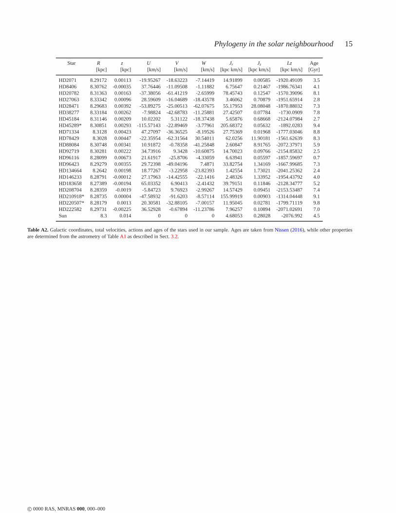
Phylogeny in the solar neighbourhood 15

Star R z U V W Jr Jz Lz Age[kpc] [kpc] [km/s] [km/s] [km/s] [kpc km/s] [kpc km/s] [kpc km/s] [Gyr]

HD2071 8.29172 0.00113 -19.95267 -18.63223 -7.14419 14.91899 0.00585 -1920.49109 3.5HD8406 8.30762 -0.00035 37.76446 -11.09508 -1.11882 6.75647 0.21467 -1986.76341 4.1HD20782 8.31363 0.00163 -37.38056 -61.41219 -2.65999 78.45743 0.12547 -1570.39096 8.1HD27063 8.33342 0.00096 28.59609 -16.04689 -18.43578 3.46062 0.70879 -1951.65914 2.8HD28471 8.29683 0.00392 -53.89275 -25.00513 -62.07675 55.17953 28.08048 -1870.88032 7.3HD38277 8.33184 0.00262 -7.98824 -42.68783 -11.25881 27.42507 0.07784 -1730.0909 7.8HD45184 8.31146 0.00209 10.02202 5.31122 -18.37438 5.65876 0.68668 -2124.07984 2.7HD45289* 8.30851 0.00293 -115.57143 -22.89469 -3.77961 205.68372 0.05632 -1892.0283 9.4HD71334 8.3128 0.00423 47.27097 -36.36525 -8.19526 27.75369 0.01968 -1777.03046 8.8HD78429 8.3028 0.00447 -22.35954 -62.31564 30.54011 62.0256 11.90181 -1561.62639 8.3HD88084 8.30748 0.00341 10.91872 -0.78358 -41.25848 2.60847 8.91765 -2072.37971 5.9HD92719 8.30281 0.00222 34.73916 9.3428 -10.60875 14.70023 0.09766 -2154.85832 2.5HD96116 8.28099 0.00673 21.61917 -25.8706 -4.33059 6.63941 0.05597 -1857.59697 0.7HD96423 8.29279 0.00355 29.72398 -49.04196 7.4871 33.82754 1.34169 -1667.99685 7.3HD134664 8.2642 0.00198 18.77267 -3.22958 -23.82393 1.42554 1.73021 -2041.25362 2.4HD146233 8.28791 -0.00012 27.17963 -14.42555 -22.1416 2.48326 1.33952 -1954.43792 4.0HD183658 8.27389 -0.00194 65.03352 6.90413 -2.41432 39.79151 0.11846 -2128.34777 5.2HD208704 8.28359 -0.0019 -5.84723 9.76923 -2.99267 14.57429 0.09451 -2153.53487 7.4HD210918* 8.28735 0.00004 -47.58932 -91.6203 -8.57114 155.99919 0.00903 -1314.04448 9.1HD220507* 8.28179 0.0013 20.30581 -32.88105 -7.00157 11.95045 0.02781 -1799.71119 9.8HD222582 8.29731 -0.00225 36.52928 -0.67894 -11.23786 7.96257 0.10894 -2071.02691 7.0Sun 8.3 0.014 0 0 0 4.68053 0.28028 -2076.992 4.5

Table A2. Galactic coordinates, total velocities, actions and ages of the stars used in our sample. Ages are taken fromNissen(2016), while other propertiesare determined from the astrometry of TableA1 as described in Sect.3.2.

c© 0000 RAS, MNRAS000, 000–000