2009PH10739-1

Cosmological Perspectives of Modified Einstein

Field Equations

R. Srivatsan 2009PH10739

Supervisor: Prof. Ajit Kumar

Abstract: The Ostrogradsky instability of higher derivative Lagrangians is derived from first principles

using Lyapunov Stability Analysis. We argue that Born-Infeld Lagrangians are viable modifications of the

Einstein-Hilbert action. The Born-Infeld (B-I) version of the FRW equations are derived and the cosmological

dynamics is studied for matter dominated closed and open universes. We compare the results with the usual

cosmology. We then investigate the quantized versions of Born Infeld electrodynamics and Born Infeld

Gravity. We derive Feynman rules for B-I electrodynamics by deriving an effective Lagrangian with the

square root removed using the Faddeev-Popov method. In the case of B-I gravity, the square root in the

Lagrangian is removed by the introduction of the Vierbien fields. This approach has the advantage that

SO(3,1) can be consistently regarded to be the gauge group of gravity. Finally, the quantum fluctuations of

the radii of spatial hypersurfaces in flat space are shown to undergo accelerated increase with time.

Email: chichieinstein@sify.com

INTRODUCTION

The light curves plotted from several hundred Type Ia supernovae [1] indicate that the

universe is expanding at an accelerated rate. In fact, the Friedmann equations derived

from Einstein‟s General Relativity, on the other hand, show that for a fluid that satisfies

the Weak Energy Condition, the universe should decelerate as it expands [2] .This

discrepancy has prompted researchers to look for phenomenological fixes for the

gravitational field equations to make theory agree with experiment.

Two choices are usually discussed at this juncture. One is to assume the existence of

an unseen dark energy [3] that presumably drives the accelerated expansion. But, in

order to make the Einstein field equation with dark matter agree with the observed

anisotropies in the cosmic microwave background, the amount of dark matter that

should be posited is eighteen times the observed ordinary matter. The implausibility of

this assumption has led to the recent interest in modifying the gravitational Lagrangian

2009PH10739-2

itself. Our aim therefore, is to investigate the possible modifications of general relativity

and their cosmological implications.

However, gravity cannot be modified in an offhand manner. There is a no-go theorem

which actually constrains the form of the Lagrangians that can be used to describe

nature. Basically, it is related to Newton‟s observation, that the equations of physics,

when written in terms of the fundamental quantities, are always second order in time [3].

This result is called Ostrogradsky‟s theorem which states that “a system whose

Lagrangian depends non-degenerately on the second and higher order derivatives of

the dynamical quantities is necessarily unstable.” The word „non-degenerately‟ means

that the higher derivatives can be solved for in terms of the lower derivatives. When this

condition is satisfied, the system has an instability.

This „theorem‟ has been invoked in the literature to support the claim that modifications

that depend on the traces of the Riemann and Ricci tensors must be excluded from

consideration [3]. But the justification of this important result has been done by bringing

ideas of second quantization into the classical setting. Moreover, the sign indefiniteness

of the energy only shows that the energy function is not a Lyapunov function. It does not

indicate that no Lyapunov function can exist. However, as we have shown, the proof

can be made more precise within classical mechanics, without discussing the particle

picture.

The quantized version of Born Infeld gravity is then investigated. For fixing ideas, the

case of Born-Infeld electrodynamics is treated. The principal difficulty in quantizing this

theory is caused by the appearance of a square root in the Lagrangian. This is removed

by the application of the Faddeev-Popov method and an effective Lagrangian is derived.

It turned out that in the case of gravity, there is a more natural procedure to remove the

square root. This is done by the introduction of Vielbien (or Tetrad) fields. The

gravitational connection then becomes a gauge field. An important point of consistency

is that throughout our work, we have been using the Palatini formalism where the metric

and connection are independent. Hence, in the language of tetrad fields, the Vielbien

(which is determined solely by the metric) and the connection (which is the gauge field)

2009PH10739-3

become independent dynamical variables. Here, we have chosen to concentrate on the

gauge field and have taken the tetrads to be those of Minkowski space where it is easier

to do quantum field theory.

THEORY AND PRINCIPLES

We briefly discuss the classical theory of general relativity. An excellent reference for

this is [2].

The field equations of general relativity can be derived from an Action principle, as was

first discovered by David Hilbert [3]. The unmodified gravitational action is given by

𝑆𝐻 = 𝑅 −𝑔 𝑑4𝑥 + 𝑆𝑀 (1)

This is called the Einstein-Hilbert Action. The 𝑅 stands for the Ricci scalar. The quantity

𝑔 represents the determinant of the metric tensor. 𝑆𝑀 represents the matter part of the

action. Two dynamical quantities enter the action given in (1). They are the metric and

the connection. The Palatini formalism results if these quantities are considered

independent degrees of freedom. We vary the action with respect to both the metric and

the connection. The explicit expression for the Ricci tensor in terms of the connection

Γ𝛽𝛾𝛼 (not necessarily a Levi-Civita connection) is given by

𝑅𝛽𝛿 = ∂αΓ𝛽𝛿𝛼 − 𝜕𝛿Γ𝛽𝛼

𝛼 + Γ𝜖𝛼𝛼 Γ𝛽𝛿

𝜖 − Γ𝜖𝛿𝛼 Γ𝛼𝛽

𝜖 (2)

The metric formalism results if we assume at the outset that the connection by default is

the Levi-Civita connection which is compatible with the metric. We vary (1) only with

respect to the metric in this case. The Levi-Civita connection is given by

Γ𝛽𝛾𝛼 =

1

2 𝑔𝛼𝛿 (𝜕𝛾𝑔𝛽𝛿 + 𝜕𝛽𝑔𝛾𝛿 − 𝜕𝛿𝑔𝛽𝛾 ) (3)

Here and in the previous equation, the repeated indices are summed. In the case of the

Einstein-Hilbert action given in (1), it can be proved [4] that the metric and the Palatini

formalism lead to the same field equations, which can be shown (after a variational

calculation) to be as given below

2009PH10739-4

𝑅𝜇𝜈 −1

2𝑔𝜇𝜈𝑅 =

8𝜋𝐺

𝑐4 𝑇𝜇𝜈 (4)

Here, 𝑇𝜇𝜈 represents the energy momentum tensor of the sources. However, this

circumstance of the metric and Palatini formalisms giving the same equations of motion

is not obtained for more general Lagrangians. For example, for the Born-Infeld Action

𝑆𝐵 = 𝜅 det 𝑔𝜇𝜈 + 𝜅𝑅𝜇𝜈 1/2

𝑑4𝑥 (5)

the metric and Palatini formalisms, give radically different equations of motion. As we

shall argue, consistency with our first result described below requires that (5) be varied

in the Palatini formalism. Varying (5) in the Palatini approach results in the following

equations of motion [5] (after varying with respect to the metric)

𝑞𝜇𝜈 = 𝑔𝜇𝜈 + 𝜅𝑅𝜇𝜈 (6)

𝑞

𝑔 𝑞𝜇𝜈 = 𝜆𝑔𝜇𝜈 − 𝜅𝑇𝜇𝜈 (7)

Here, 𝑞𝜇𝜈 represents an auxiliary metric while 𝑞𝜇𝜈 represents its inverse. 𝜅 is a coupling

constant while 𝜆 is a Cosmological constant. 𝑞 and |𝑔| are the determinants of 𝑞𝜇𝜈 and

𝑔𝜇𝜈 respectively. The variation with respect to the connection yields the following

equation

Γ𝛽𝛾𝛼 =

1

2 𝑞𝛼𝛿 (𝜕𝛾𝑞𝛽𝛿 + 𝜕𝛽𝑞𝛾𝛿 − 𝜕𝛿𝑞𝛽𝛾 ) (8)

On the other hand, varying (5) in the metric formalism yields the following mess

−𝜅𝑇𝜇𝜈 =

−1

2𝐹𝑔𝜇𝜈 + 𝑔𝜇𝜈 𝜕𝛼𝜕

𝛼 − ∇𝜇∇𝜈 𝐹𝑅 + 𝐹𝑅𝑅𝜇𝜈 + 2∇𝛼∇𝜇 𝐹𝑅𝑅𝜈𝛼 − 𝑔𝜇𝜈∇𝛽∇𝛼 𝐹𝑅𝑅

𝛼𝛽 −

𝜕𝛼𝜕𝛼 𝐹𝑅𝑅𝜇𝜈 − 2𝐹𝑅𝑅𝜈

𝛼𝑅𝜇𝛼 + 𝑔𝜇𝜈 𝜕𝛼𝜕𝛼 𝐹𝑅𝑅 − ∇𝜇∇𝜈 𝐹𝑅𝑅 + 𝐹𝑅𝑅𝑅𝜇𝜈 + …

The other quantities need not be defined as they are not used in the subsequent

discussion.

2009PH10739-5

Our work on the quantum version of B-I electrodynamics and gravity uses some new

tools which are briefly summarized here.

The Faddeev Popov [12] method uses the path integral formalism to remove redundant

infinities while performing the integral. The procedure is as follows:

The generating functional for a Quantum Field theory that is gauge invariant is given by

𝑍 = 𝐷𝐴𝜇 𝑒𝑖𝑆 (9)

Here 𝑆 is the action evaluated along a particular path in the space of the gauge field.

Since the action is gauge invariant, the generating functional above involves sums over

fields that are related to each other by gauge transformations. This over counting results

in infinities. The way to fix this is to insert unity in the form:

Δ𝐹−1 𝐴𝜇 = 𝐷𝑈 𝛿(𝐹𝑎(𝐴𝜇

𝑈)) (10)

Here, 𝐹𝑎 𝐴𝜇𝑈 = 0 is the gauge condition one would like to impose. 𝑈 is a gauge group

element, 𝐷𝑈 represents integration over the group elements. 𝛿 represents the delta

functional and 𝑎 represents a color index (in case of SU(2)). As argued in [12], the

quantity given above is gauge invariant. Finally, writing 1 as 1 = Δ𝐹(𝐴𝜇 ) 𝐷𝑈 𝛿(𝐹𝑎(𝐴𝜇𝑈))

in the generating functional, we get

𝑍 = 𝐷𝑈 𝐷𝐴𝜇 𝑒𝑖𝑆 Δ𝐹(𝐴𝜇 )𝛿(𝐹𝑎(𝐴𝜇 )) (11)

Thus the integral over the group space only contributes an overall multiplicative

constant and hence can be ignored. The correct expression is therefore,

𝑍 = 𝐷𝐴𝜇 𝑒𝑖𝑆 Δ𝐹(𝐴𝜇 )𝛿(𝐹𝑎(𝐴𝜇 )) (12)

This Δ𝐹(𝐴𝜈) is the origin of the famous Faddeev-Popov ghosts. However since the

gauge group of Electrodynamics is Abelian, this term is independent of the 𝐴𝜇 in this

case and hence can be taken out of the integral.

Another tool that is subsequently required is the Vielbien (or Tetrad) formalism for the

gravitational field. In the usual formulation of gravity, the dynamical field is taken to be

2009PH10739-6

the metric 𝑔𝜇𝜈 and the connection as stated above is the Levi-Civita connection Γ𝛽𝛾𝛼 .

We have used here the Palatini formalism that considers these quantities to be

independent. An equivalent approach to gravity would be the introduction of the Tetrad

fields 𝑒𝑎𝜇

[13,14] which have both a spacetime index 𝜇 and an internal index 𝐼. They are

defined to satisfy the following relation

𝜂𝐼𝐽 = 𝑔𝜇𝜈 𝑒𝐼𝜇𝑒𝐽𝜈 (13)

Here 𝜂𝑎𝑏 is the Minkowski metric. This equation is then inverted to obtain the following

equation which is also used as a general definition of the Cotetrad fields

𝑔𝜇𝜈 = 𝜂𝐼𝐽𝑒𝜇𝐼𝑒𝜈

𝐽 (14)

The internal indices of the Tetrad transform in such a way that the tensor 𝜂𝐼𝐽 is left

invariant. As we know, the set of all such transformations is precisely the Lorentz Group

SO(3,1). Hence, in a particular coordinate system, we treat gravity as a gauge theory

with the gauge group SO(3,1). The transformation is given by

𝑒𝜇𝐼′ (𝑥) = Λ𝐽

𝐼′ (𝑥)𝑒𝜇𝐽 (𝑥) (15)

Here, Λ𝐽𝐼′ is an element of SO(3,1) and as seen above it depends explicitly on the

spacetime point at which it is carried out since it is a local gauge transformation in the

theory. The analogue of the Riemann tensor here is the “field strength” of a gauge field

𝐴𝛼𝐼𝐽

and in perfect analogy to the Yang-Mills field is given by [13]

𝐹𝛼𝛽𝐼𝐽 = 𝜕𝛼𝐴𝛽

𝐼𝐽 − 𝜕𝛽𝐴𝛼𝐼𝐽 + 𝐴𝛼 ,𝐴𝛽

𝐼𝐽

= 𝜕𝛼𝐴𝛽𝐼𝐽− 𝜕𝛽𝐴𝛼

𝐼𝐽+ 𝑐𝑃𝑄𝑅𝑆

𝐼𝐽𝐴𝛼𝑃𝑄𝐴𝛽𝑅𝑆 (16)

where, 𝑐𝑃𝑄𝑅𝑆𝐼𝐽

are the structure constants of the SO(3,1) group. Once we have the field

strength 𝐹𝛼𝛽𝐼𝐽

, the Riemann and Ricci tensors can be defined as follows

𝑅𝛾𝛿𝛼𝛽

= 𝐹𝛾𝛿𝐼𝐽 𝑒𝐼

𝛼𝑒𝐽𝛽 (17)

2009PH10739-7

Finally, we review a theorem from control theory. This result is very important for the

subsequent discussion with regard to the proof of the Ostrogradsky instability.

Consider the following system of differential equations

𝒙 = 𝑓(𝒙) (18)

Here, 𝒙 represents an n-dimensional vector, while 𝑓(𝒙) is a scalar point function. The

dot represents a time derivative. Without losing generality, we can assume that 𝒙 = 0 is

the equilibrium point of the system [6]. We now state the result. The proof can be looked

up in [6].

Chaetev‟s Theorem [6] Let 𝒙 = 0 be an equilibrium point for (1). Let 𝑉 ∶ 𝐷 → 𝑅 be a

continuously differentiable function such that 𝑉 0 = 0 and 𝑉 𝒙0 > 0 for some 𝒙𝟎 with

arbitrarily small | 𝒙0 |. For 𝑟 > 0, let 𝐵𝑟 denote the set 𝑥 ϵ Rn 𝐱 ≤ r} contained in 𝐷

and let

𝑈 = 𝒙 𝜖 𝐵𝑟 𝑉 𝒙 > 0} (19)

With 𝑈 defined as in (10), suppose that 𝑉 > 0 throughout 𝑈. Then, the point 𝒙 = 0 is

unstable.

Here, the instability referred to, is instability in the Lyapunov sense. When translated in

terms of the particle picture, this amounts to exactly the same sense as conveyed in [3].

However, this result is more general and can be applied even to a classical field theory,

like General Relativity, which cannot be quantized unambiguously at present. Now, we

apply this result to the case of the system with a Lagrangian that depends non-

degenerately on the second and higher order derivatives of the dynamical quantities.

For simplicity and without loss of generality, we treat below the case of a system with a

finite number of degrees of freedom.

RESULTS AND DISCUSSION

Part 1 of the Thesis:

2009PH10739-8

Proof of Ostrogradsky instability: In [3], the Ostrogradsky Hamiltonian for one degree of

freedom has been constructed explicitly for a higher derivative Lagrangian 𝐿(𝑞, 𝑞 , 𝑞 ) to

be of the following form

𝐻 𝑞1,𝑞2,𝑝1,𝑝2 = 𝑝1𝑞2 + 𝜇 𝑞1,𝑞2,𝑝2 − 𝐿(𝑞1, 𝑞2, 𝜇) (20)

Here, the choice of canonical coordinates is as follows [3]:

𝑞1 = 𝑞, 𝑝1 =𝜕

𝜕𝑞 𝐿 −

𝑑

𝑑𝑡

𝜕𝐿

𝜕𝑞

𝑞2 = 𝑞 , 𝑝2 =𝜕

𝜕𝑞 𝐿 (21)

An approach to proving the instability of a system was already carried out in [7], in the

context of charged solitons. The ideas presented below are a combination of the steps

taken in that paper together with the result quoted above.

Now, we come to the crux of the result. Phase space translations are canonical

transformations [8]. Therefore, by a suitable canonical transformation, the Hamiltonian

can be thrown into the following form:

𝐻 𝑄,𝑃 = 𝑄1𝑃2 + 𝑕 𝑄,𝑃 (22)

Here, 𝑕(𝑄,𝑃) is a function that contains no linear terms. Therefore, in a neighborhood

of the origin, the first term dominates. Now, if we choose the Chaetev‟s function as

𝑉 𝑄,𝑃 = 𝑄1𝑄2, we get for the derivative of this function along the solution trajectories

𝑉 = 𝑄1 𝑄2 + 𝑄1𝑄2

, so that, using the equations of motion contained in (22),

𝑉 = 𝑄12 + 𝑢(𝑄,𝑃) (23)

Again, the function 𝑢 𝑄,𝑃 is dominated by the first term in a neighborhood of the origin.

Therefore, in a small neighborhood around the origin, the conditions of Chaetev‟s

theorem are satisfied so that this theory is unstable at the origin. Finally, by a suitable

translation, we can reach the same conclusion at any point of the trajectory. Hence, we

conclude that such a theory is unstable everywhere.

2009PH10739-9

Now that we have shown that any higher derivative Lagrangian is unstable in the

Lyapunov sense, we can return to the question of modifying gravity to explain

accelerated expansion. In the literature, 𝑓(𝑅) modifications are discussed very

extensively, where 𝑅 is the Ricci scalar [3], [9]. It is claimed that no other non-trivial

modification can satisfy the constraints imposed by the result proved above [3].

However, Born-Infeld (B-I) Lagrangians are particularly attractive because of their

intriguing properties [10].

The B-I Lagrangian made its appearance with the modification of the electrodynamic

action by Born and Infeld. This was done to remove the infinite self energy of point

charges by introducing an upper bound on the magnitude of the electric field. It was

further pointed out that the B-I electromagnetic field propagates without birefringence

[10]. Analogous work has been carried out for the case of the gravitational field.

However, the cosmology discussed has been restricted to the case where the spatial

hyperspaces are flat [11]. We have extended these results to the case where the spatial

hyperspaces can be curved. Before proceeding further, we must mention here an

important consequence of the Ostrogradsky instability.

The Born Infeld action in (5) can only be varied in the Palatini approach: This

statement can be justified by referring to (2), (3) and (5). Suppose (5) is varied in the

metric formalism. Then as stated in the introduction, the connection is fixed as the Levi

Civita connection given in (3). In that case, the determinant in (5), can be expanded in

terms of the trace as follows (upto third order):

det 𝑔𝜇𝜈 + 𝜅𝑅𝜇𝜈 ≅ 1 +1

2𝜅(𝑅 − 𝜅𝐾 − 𝜅2𝑆) (24)

where

𝐾 = 𝑅𝜇𝜈𝑅𝜇𝜈 −

1

2𝑅2 and 𝑆 = 8𝑅𝜇𝜈𝑅𝜇𝛼𝑅𝜈

𝛼 − 6𝑅𝑅𝜇𝜈𝑅𝜇𝜈 + 𝑅3 (25)

Therefore, if the metric is considered the sole dynamical quantity, the Lagrangian would

involve the second and higher derivatives of the metric. But this would result in an

unstable theory in accordance with the result proved above.

2009PH10739-10

However, in the Palatini case, only the first derivatives of the connection coefficients

appear in the expression for the Ricci tensor as can be seen from (2). Therefore, in this

case, there is no instability provided the action in (5) is varied by taking the metric and

connection as separate degrees of freedom and therefore, Born-Infeld Lagrangians are

also viable as alternative theories of gravity.

The FRW equations in Born Infeld Gravity: With the question of viability settled, we

can now set up and solve the FRW equations for B-I gravity. We generalize here the flat

space results of [11] to curved spatial hyper surfaces.

As usual, we assume that the universe is homogenous and isotropic. This results in the

following ansatz for the metric in comoving coordinates [2]

𝑔𝜇𝜈 𝑑𝑥𝜇𝑑𝑥𝜈 = − 𝑑𝑥0 2 + 𝑎 𝑡 2

𝑑𝑟 2

1−𝑘𝑟2 + 𝑟2 𝑑𝜃 2 + sin2 𝜃 𝑑𝜙 2 (26)

Here, a(t) is the cosmic radius. Other symbols have their usual meanings. For the B-I

equations, we also need an ansatz for the auxiliary metric 𝑞𝜇𝜈 . This is at once supplied

by the demand for homogeneity and isotropy as [6]

𝑞00 = −𝑈 𝑡 2 and 𝑞𝑖𝑗 = 𝑉 𝑡 2𝛾𝑖𝑗 (27)

Here, 𝛾𝑖𝑗 represents the spatial components of the metric. Equation (27) together with

(8) then determines the non-zero connection coefficients as (here, U‟ represents a time

derivative)

Γ𝑡𝑡𝑡 =

𝑈 ′

𝑈 Γ𝑟𝑟

𝑡 =𝑎2𝑉𝑉 ′

1−𝑘𝑟2 𝑈2+

𝑎𝑎 ′𝑉2

1−𝑘𝑟2 𝑈2 (28)

Γ𝜃𝜃𝑡 =

𝑎2𝑉𝑉 ′

𝑈2+

𝑎𝑎 ′𝑉2

𝑈2 Γ𝜙𝜙

𝑡 = Γ𝜃𝜃𝑡 sin2 𝜃 (29)

Γ𝑟𝑟𝑟 =

𝑘𝑟

1−𝑘𝑟2 Γ𝜃𝜃𝑟 = −𝑟 1− 𝑘𝑟2 Γ𝜙𝜙

𝑟 = Γ𝜃𝜃𝑟 sin2 𝜃 (30)

Γ𝜙𝜙𝜃 = − sin𝜃 cos 𝜃 Γ𝜙𝜃

𝜙= cot 𝜃 (31)

Γ𝜃𝑟𝜃 = Γ𝜙𝑟

𝜙=

1

𝑟 (32)

2009PH10739-11

Γ𝑟𝑡𝑟 = Γ𝜃𝑡

𝜃 = Γ𝜙𝑡𝜙

= 𝑎 ′

𝑎+

𝑉 ′

𝑉 (33)

For use in (6), we also need the 𝜇𝜈 = 00 and 11 components of the Ricci tensor, which

are given by (as usual an apostrophe represents a time derivative)

𝑅00 = 3𝐻1 𝐻 + 𝐻2 − 6𝐻𝐻2 − 3 𝑎 ′′

𝑎+

𝑉 ′′

𝑉 (34)

𝑅11 =1

1−𝑘𝑟2 2𝑘 +

𝑎2

𝑈2 2𝐻𝑉𝑉 ′ + 𝑉 ′2 + 𝑉𝑉 ′′ + 𝑉2 𝐻2 +

𝑎 ′′

𝑎 + 𝑉𝑉 ′ + 𝐻𝑉2 𝐻 + 𝐻1 −

𝐻2 (35)

Here 𝐻 =𝑎 ′

𝑎,𝐻1 =

𝑈 ′

𝑈,𝐻2 =

𝑉 ′

𝑉

For the matter distribution, we assume a perfect fluid with pressure 𝑝 and density 𝜌. It

can further be shown that the fluid satisfies the equation of continuity. Finally, we can

write the following equations of motion using (6) and (7)

1 − 𝑈2 = 𝜅 3𝐻1 𝐻 + 𝐻2 − 6𝐻𝐻2 − 3 𝑎 ′′

𝑎+

𝑉 ′′

𝑉 (36)

𝑉2 − 1 =2𝑘𝜅

𝑎2 +𝜅

𝑈2 {2𝐻𝑉𝑉 ′ + 𝑉 ′2 + 𝑉𝑉 ′′ + 𝑉2 𝐻2 +𝑎 ′′

𝑎 + 𝑉𝑉 ′ + 𝐻𝑉2 𝐻 + 𝐻1 − 𝐻2 }

(37)

𝑈𝑉 = 𝜆 + 𝜅𝑝 (38)

𝑉3

𝑈= 𝜆 + 𝜅𝜌 (39)

The fluid also has an equation of state that is given by the following relation

𝑝 = 𝑤𝜌 (40)

Finally, the continuity equation can be written as

𝜌 ′

𝜌= −3𝐻 1 + 𝑤 (41)

2009PH10739-12

We can immediately integrate (41) to yield the density as a function of radius

𝜌 = 𝜌0𝑎−3 1+𝑤 (42)

Here, 𝑤 is a constant that determines the kind of fluid that is present in the universe. It

is 0 for matter, -1 for vacuum and -1/3 for radiation. The second derivatives can be

eliminated between (36) and (37). Moreover, (38) and (39) can be solved to give 𝑈 and

𝑉 as a function of 𝜌 and hence as a function of 𝑎(𝑡) as follows

𝑉 = 𝜆 + 𝜅𝑤𝜌0𝑎−3 1+𝑤

1

4 𝜆 + 𝜅𝜌0𝑎−3 1+𝑤

1

4 (43)

𝑈 = 𝜆+𝜅𝑤𝜌0𝑎

−3 1+𝑤 34

𝜆+𝜅𝜌0𝑎−3 1+𝑤 14

(44)

After doing all the manipulations, we end up with the following first order equation for 𝑎

𝐻 =𝑎 ′

𝑎=

± 𝛼2+ 4 𝛼2+ 2𝛽+2 +𝛼𝛽 – 𝛼 𝑈

𝑉

2 𝑎2

𝜅 𝑉2−1 −2𝑘 +

(𝑈2−1)

3𝜅 −𝛼

2 𝛼2+ 2𝛽+2 +𝛼𝛽 – 𝛼 (45)

Here

𝛼 = −3𝜅𝜌 𝑎 1 + 𝑤

4

𝑤

𝜆 + 𝜅𝑤𝜌 𝑎 +

1

𝜆 + 𝑤𝜌 𝑎

𝛽 = −3𝜅𝜌 𝑎 1 + 𝑤

4

3𝑤

𝜆 + 𝜅𝑤𝜌 𝑎 −

1

𝜆 + 𝑤𝜌 𝑎

Equation (45) is therefore the final result of our work for the first part of the thesis. It

gives an equation for the evolution of 𝑎(𝑡). This can be used to discuss any differences

or similarities with the equation for the Hubble rate 𝑎 ′

𝑎 in Einstein‟s relativity. This

equation was simulated using the odeint routine in SciPy and the results are shown

below.

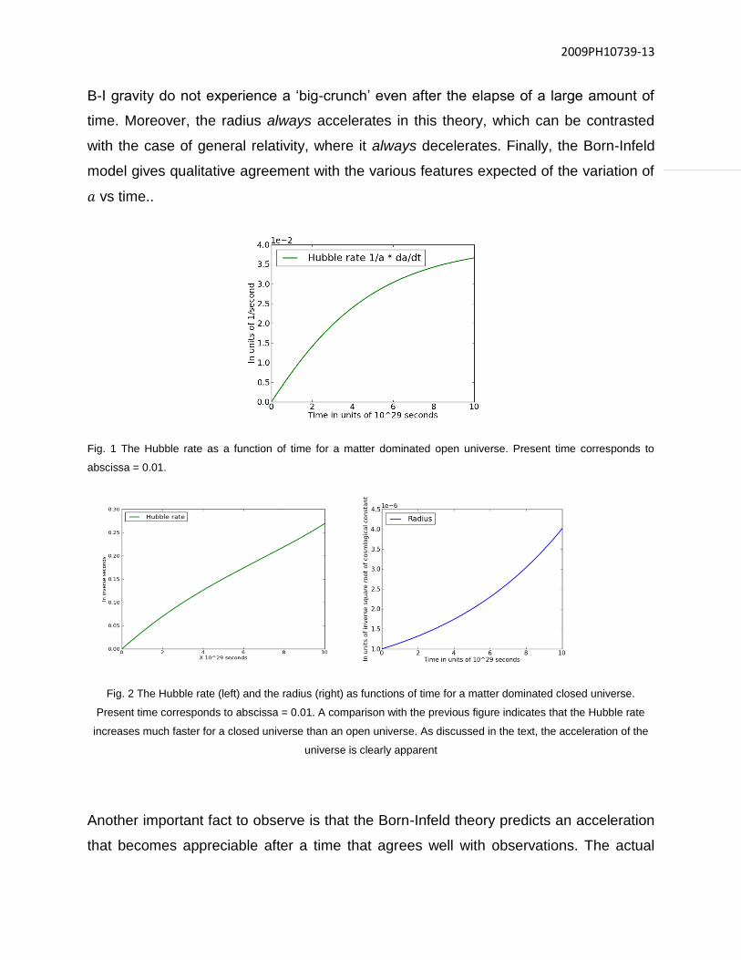
As illustrated in Figure 1 and 2, the main point of difference between the solutions of the

FLRW equations in Einstein‟s gravity and in the present case is that closed universes in

2009PH10739-13

B-I gravity do not experience a „big-crunch‟ even after the elapse of a large amount of

time. Moreover, the radius always accelerates in this theory, which can be contrasted

with the case of general relativity, where it always decelerates. Finally, the Born-Infeld

model gives qualitative agreement with the various features expected of the variation of

𝑎 vs time..

Fig. 1 The Hubble rate as a function of time for a matter dominated open universe. Present time corresponds to

abscissa = 0.01.

Fig. 2 The Hubble rate (left) and the radius (right) as functions of time for a matter dominated closed universe.

Present time corresponds to abscissa = 0.01. A comparison with the previous figure indicates that the Hubble rate

increases much faster for a closed universe than an open universe. As discussed in the text, the acceleration of the

universe is clearly apparent

Another important fact to observe is that the Born-Infeld theory predicts an acceleration

that becomes appreciable after a time that agrees well with observations. The actual

2009PH10739-14

variation of the cosmic radius and Hubble rate predicted by the B-I gravity is given

below. Therefore, by tuning the values of the coupling constant 𝜅 and the cosmological

constant 𝜆 properly, one can, in principle, make the actual values of the radius agree

with the experiment. On the other hand, an advantage of 𝑓(𝑅) modifications is that any

history of the evolution of the universe can be supported by a proper choice of the

function 𝑓(𝑅) [3]. This flexibility has been lost in the case of the Born-Infeld modification.

Nevertheless, as the preceding plots show, the history predicted by our calculations is

to a tolerable extent, consistent with observations. Figure 2 above illustrates the major

differences between conventional cosmology and B-I cosmology which were mentioned

earlier. In addition to the points indicated above, we also observe that closed universes

always accelerate. This is evident from the fact that the Hubble rate keeps on

increasing. Moreover, we have finally achieved our goal : to show that B-I cosmologies

give believable results as far as cosmology is concerned and give a natural framework

to explain the observed accelerated expansion of the universe. Moreover, as discussed

above, the tuning of the coupling constants and the cosmological constant can make

the results agree with any observed value of the acceleration.

Part 2 of the thesis:

The Quantisation of the Born-Infeld Electrodynamical Field:

The Lagrangian density for the B-I field is given by:

𝐿 = 1 +𝐹𝜇𝜈 𝐹

𝜇𝜈

𝛽2 −𝐹𝜇𝜈 𝐵

𝜇𝜈 𝐹𝜇𝜈 𝐵𝜇𝜈

𝛽4 1/2

(46)

Here, 𝛽 is a free parameter of the theory. Moreover, 𝐹𝜇𝜈 is the field strength and 𝐵𝜇𝜈 is

the dual of the field strength.

In order to remove the square root, we introduce an auxiliary field 𝜉 after [15] as follows:

𝐿 = −𝜉

2 1 +

𝐹𝜇𝜈 𝐹𝜇𝜈

𝛽2 +𝐹𝜇𝜈 𝐵

𝜇𝜈 𝐹𝜇𝜈 𝐵𝜇𝜈

𝛽4 −1

2𝜉 (47)

We observe that the 𝜉 field enters the Lagrangian without time derivatives and hence, it

has no independent dynamics. Its equations of motion are given by

2009PH10739-15

𝜕

𝜕𝜉𝐿 = 0 = −

1

2 1 +

𝐹𝜇𝜈 𝐹𝜇𝜈

𝛽2+

𝐹𝜇𝜈 𝐵𝜇𝜈 𝐹𝜇𝜈 𝐵

𝜇𝜈

𝛽4 +

1

2𝜉2= 0 (48)

This fixes 𝜉 in terms of the original dynamical fields which when substituted in the

Lagrangian, gives the same equation as the original one.

The advantage of introducing this field is that on passing to the path integral, 𝜉 can be

taken to be independent of the other fields, since in the path integral, the action is not

stationary but acquires all values with same probability.

The Faddeev-Popov procedure is then used here, and consists of exploiting the gauge

invariance to factor out the infinite volume of the Gauge space as discussed in the

Theory section. For the Abelian case of electrodynamics, this throws in a factor that is

independent of the 𝐴𝜈 and is not important for our approach. After doing all that, the

normal course is to insert an arbitrary field 𝑐 and averaging over all such fields. In our

approach, we choose as 𝑐 the extra auxiliary field which we have introduced in the

Lagrangian above. The argument for justifying this is given below:

Proof: The path integral (or the generating functional) is given by:

𝑍 = 𝐷𝜉 𝐷𝐴𝜈 𝑒𝑖𝑆 𝜉 ,𝐴𝜈 (49)

Since 𝜉 and 𝐴𝜈 are independent degrees of freedom, we can proceed with the standard

F-P integration for 𝐴𝜈 to get

𝑍 = 𝐷𝜉 𝐷𝐴𝜈 Δ𝐹 𝐴𝜈 𝛿 𝑔 𝐴𝜈 − 𝑐 𝑒𝑖𝑆 𝜉 ,𝐴𝜈 (50)

Here, Δ𝐹[𝐴𝜈 ] is the term arising out of neglecting the infinite volume element of the

gauge group space. For Abelian gauge theory, it is independent of 𝐴𝜈 and can be taken

out of the integral. Also, 𝑔(𝐴𝜇 ) is the gauge fixing condition that one would like to

impose.

The important point to observe here is that the arbitrary field 𝑐 introduced above is

completely independent of 𝐴𝜈 . Therefore, it can be taken to be 𝜉 itself. The justification

for this is that there is gauge invariance in the equations. This freedom can be used to

set the gauge function 𝑔 𝐴𝜇 equal to any arbitrary function. Explicitly,

2009PH10739-16

𝐴′𝜇 = 𝐴𝜇 + 𝜕𝜇𝜆

so that, if 𝜕𝜇𝐴𝜇 = 0, then, 𝑔 𝐴𝜇 ′ = 𝜕𝜇𝐴

𝜇 ′ = 𝜕𝜇𝜕𝜇𝜆 = 𝜉 which can be solved for 𝜆. Thus

in the path integral, the gauge fixing function can be set equal to 𝜉.

The main point of difference is that instead of the traditional gauge breaking term in the

effective Lagrangian, which is quadratic in the 𝑔(𝐴𝜈), we get the following effective

Lagrangian after integrating over the 𝜉.

𝐿𝑒𝑓𝑓 = −𝑔 𝐴𝜈

2 1 +

𝐹𝜇𝜈 𝐹𝜇𝜈

𝛽2 − 𝐹𝜇𝜈 𝐵𝜇𝜈

2

𝛽4 −1

2𝑔 𝐴𝜈 (51)

Finally, since as we said above, the auxiliary field 𝜉 is not dynamical, we can restrict to

variations of the Lagrangian such that 𝛿 𝑔 𝐴𝜇 = 0. Therefore, the first and last terms

can be neglected to get

𝐿𝑒𝑓𝑓 = 𝑔 𝐴𝜇

2 𝐹𝜇𝜈 𝐹

𝜇𝜈

𝛽2 − 𝐹𝜇𝜈 𝐵𝜇𝜈

2

𝛽4 (52)

Hence, we have achieved our aim: we have removed the square root and brought the

Lagrangian to polynomial form in the 𝐴𝜇and their derivatives. Now, we come to the

problem of getting the Feynman rules for this effective Lagrangian.

The Feynman Rules for Born-Infeld Electrodynamics

Using the effective Lagrangian derived above, we now give the derivation of the

Feynman rules for B-I Electrodynamics.

𝐿𝑒𝑓𝑓 =𝜕𝜈𝐴

𝜈

2 𝐹𝜇𝜈 𝐵

𝜇𝜈 2

𝛽4 + 𝐹𝜇𝜈 𝐹

𝜇𝜈

𝛽2 (53)

The effective action is given by

𝑆𝑒𝑓𝑓 =1

2 𝜕𝛼𝐴

𝛼 𝐹𝜇𝜈 𝐵

𝜇𝜈 2

𝛽4 + 𝐹𝜇𝜈 𝐹

𝜇𝜈

𝛽2 𝑑4𝑥 (54)

Assuming the vector fields go to zero at infinity, we can use integration by parts to

rewrite this as follows:

2009PH10739-17

𝑆𝑒𝑓𝑓 = −1

2 𝐴𝛼𝜕𝛼

𝐹𝜇𝜈 𝐵𝜇𝜈

2

𝛽4 +

𝐹𝜇𝜈 𝐹𝜇𝜈

𝛽2 𝑑4𝑥

= −1

2 𝐴𝛼

𝐹𝜇𝜈 𝐵𝜇𝜈 𝜕𝛼 𝐹𝜇𝜈 𝐵

𝜇𝜈

𝛽4 + 𝜕𝛼𝐹𝜇𝜈 𝐹

𝜇𝜈

𝛽2 𝑑4𝑥 (55)

Here, we would like to define a few symbols before proceeding further; we define

𝜖𝜇1𝜈1

𝜇𝜈 to represent the quantity that is +1 for (𝜇1𝜈1) = (𝜇𝜈) and -1 for the cyclic

permutation. 𝜖𝛼𝛽𝛾𝛿 is the usual permutation tensor defined for four indices. With these

definitions, the action above becomes

𝑆𝑒𝑓𝑓 = − 𝐴𝛼

𝛽4 𝜖𝜇𝜈𝛾𝛿 𝐹

𝜇𝜈𝐹𝛾𝛿 𝜕𝛼 𝜖𝜇1𝜈1𝛾𝛿𝐹𝜇1𝜈1𝐹𝛾𝛿 +

𝐴𝛼

𝛽2 𝐹𝜇𝜈 𝜕𝛼𝐹𝜇𝜈 𝑑4𝑥

(56)

Renaming a few indices, and expanding, we get the integrand

𝐴𝛼

𝛽4 𝜖𝜇𝜈𝛾𝛿 𝜖𝜇1𝜈1 𝜇𝜈

𝜖𝜍1𝜌1 𝛾𝛿

𝜕𝜇1𝐴𝜈1𝜕𝜍1𝐴𝜌1 𝜕𝛼 𝜖𝜇1𝜈1𝛾𝛿 𝜖𝜂𝜃𝜇1𝜈1𝜖𝛾1𝛿1

𝛾𝛿𝜕𝜂𝐴𝜃𝜕𝛾1𝐴𝛿1 𝑑4𝑥

+ 𝐴𝛼

𝛽2 𝜖𝜇1𝜈1 𝜇𝜈

𝜖𝜇𝜈 𝛼1𝛽1 𝜕𝜇1𝐴𝜈1𝜕𝛼𝜕𝛼1

𝐴𝛽1 𝑑4𝑥 (57)

We thus see that the effective action consists of two terms. One which is third order in

the field (the second term) and another which is fifth order in the field (the first term).

Writing the 𝐴 field in terms of its Fourier components, i.e.,

𝐴𝛽 𝑥𝜇 = 𝐴𝛽 𝑝𝜇 exp(𝑖𝑝𝜇𝑥𝜇 ) 𝑑4𝑝 (58)

we get for the second term in the equation above :

𝑆2𝑒𝑓𝑓= −𝑖

𝐴𝛼 𝑝1 𝜖𝜇1𝜈1

𝜇𝜈𝜖𝜇𝜈𝛼1𝛽1𝑝2

𝜇1𝐴𝜈1 𝑝2 𝑝3𝛼𝑝3𝛼1

𝐴𝛽1 𝑝3

exp(𝑖 𝑝1 + 𝑝2 + 𝑝3 𝜇𝑥𝜇 )𝑑4𝑝1𝑑

4𝑝2𝑑4𝑝3𝑑

4𝑥 (59)

The integration over the 𝑥 coordinates gives a delta function. Finally, finding the

functional derivatives [12] with respect to the 𝐴(𝑝), we get the amplitude in

momentum space for this coupling to be (i.e., the Feynman Rule for this three-

field vertex)

2009PH10739-18

𝛿3𝑆2𝑒𝑓𝑓

𝛿𝐴 𝑝1 𝛿𝐴 𝑝2 𝛿𝐴 𝑝3 = −

𝑖

𝛽2 𝛿 𝑝1 + 𝑝2 + 𝑝3 𝜖𝜇1𝜈1

𝜇𝜈𝜖𝜇𝜈𝛼1𝛽1𝑝2

𝜇1𝑝3𝛼𝑝3𝛼1

+ 𝑝𝑒𝑟𝑚𝑢𝑡𝑎𝑡𝑖𝑜𝑛𝑠

(60)

The permutations arise because the fields are indistinguishable. An important point of

difference from the Yang-Mills propagator is that the coupling amplitude is cubic in the

momentum while it is linear there; this in itself points to the intense self coupling that

occurs in our case.

Similarly the fifth order terms which occur in the first term can be handled using Fourier

Transformations to get:

𝛿5𝑆1𝑒𝑓𝑓

𝛿𝐴 𝑝1 𝛿𝐴 𝑝2 𝛿𝐴 𝑝3 𝛿𝐴 𝑝4 𝛿𝐴 𝑝5 = −

𝑖

𝛽4𝛿 𝑝1 + 𝑝2 + 𝑝3 + 𝑝4 + 𝑝5

𝜖𝜇𝜈𝛾𝛿 𝜖𝜇1𝜈1

𝜇𝜈𝜖𝜍1𝜌1

𝛾𝛿𝜖𝜇1𝜈1𝛾𝛿 𝜖𝜂𝜃

𝜇1𝜈1𝜖𝛾1𝛿1 𝛾𝛿

𝑝2𝜇1𝑝3

𝜍1𝑝4𝜂𝑝5𝛾1 𝑝4𝛼 + 𝑝5𝛼 + 𝑝𝑒𝑟𝑚𝑢𝑡𝑎𝑡𝑖𝑜𝑛𝑠

(61)

The Quantisation of Born-Infeld Gravity:

Having disposed of the Electrodynamics case, we now come to the treatment of gravity.

Here, there is a natural way in which the square root in the Lagrangian can be removed.

This is achieved as stated in the theory section, by employing Tetrad fields. In terms of

the tetrads, as shown in [16], the Lagrangian for B-I gravity is given by

𝑆 = 𝜆4 𝑑4𝑥 𝑒 + 𝜆3 𝑑4𝑥 𝑒 𝑅 +𝜆2

2! 𝑑4𝑥 𝑒 𝑅2 − 𝑅𝜇𝜈𝑅

𝜇𝜈

+𝜆

3! 𝑑4𝑥 𝑒 𝑅3 − 3𝑅𝑅𝜇𝜈𝑅𝜇𝜈 + 2𝑅𝜇𝛼𝑅𝛼𝛽𝑅𝜇

𝛽 + 𝑑4𝑥 𝑒 det𝑅𝜇𝜈

(62)

Here, 𝑒 = −𝑔 = det 𝑒𝛼𝜇, 𝑅 is the Ricci scalar, 𝑅𝜇𝜈 is the Ricci tensor. Finally 𝜆 =

2

Λ is

related to the reciprocal of the cosmological constant. We now present below the

arguments used in deriving the analogy to the Yang-Mills field.

2009PH10739-19

Analogy with the Yang-Mills field:

First we start with the observation that the cosmological constant is very small in value.

Thus only the leading order terms in 𝜆 in the Lagrangian above need to be taken into

account.

Moreover, since we are using the Palatini formalism, the Tetrad 𝑒𝛼𝜇 and the connection

𝐹𝛼𝛽𝐼𝐽

are independent. Since the signature of gravity is contained in the derivatives of the

connection and not in the metric, we assume here that the 𝑒𝛼𝜇 are non-dynamical and

have been fixed as the Tetrads of some convenient background metric (Minkowski

spacetime in our case). Thus, the first term in the action above is irrelevant. Since we

are interested in two-point correlation functions, the second term can also be neglected.

Finally, the fourth and fifth terms are ignored because of the smallness of the

cosmological constant argument above.

The interesting term is therefore, given by

𝑆 =𝜆2

2! 𝑑4𝑥 𝑅2 − 𝑅𝜇𝜈𝑅

𝜇𝜈 (63)

where 𝑒 = det 𝑒𝛼𝜇 = 1 since the Tetrads are those of flat spacetime. 𝑅𝜇𝜈 𝑅𝜇𝜈 can be

written in terms of the connection as

𝑅𝜇𝜈𝑅𝜇𝜈 = 𝑒𝑎𝜍𝑒𝑐

𝛾 𝐹𝑑𝛾𝑎𝜌𝐹𝜌𝜍𝑐𝑑 (64)

The product of the Tetrads can be decomposed as

𝑒𝑎𝜍𝑒𝑐

𝛾=

1

4𝑔𝜍𝛾𝜂𝑎𝑐 + 𝐴𝑎𝑐

𝜍𝛾 (65)

Here, 𝐴𝑎𝑐𝜍𝛾

is some tensor that depends on the metric. The only condition that should be

satisfied by this tensor is that 𝑔𝜍𝛾𝐴𝑎𝑐𝜍𝛾

= 0. If this holds, then

𝑔𝜍𝛾𝑒𝑎𝜍𝑒𝑐

𝛾= 𝜂𝑎𝑐 + 𝑔𝜍𝛾𝐴𝑎𝑐

𝜍𝛾= 𝜂𝑎𝑐 (66)

With this decomposition, the second term in the Lagrangian can be written as

2009PH10739-20

𝑅𝜇𝜈𝑅𝜇𝜈 =1

4𝑔𝜍𝛾𝜂𝑎𝑐𝐹𝑑𝜍

𝑎𝜌𝐹𝜌𝜍𝑐𝑑 + 𝐴𝑎𝑐

𝜍𝛾 𝐹𝑑𝛾𝑎𝜌𝐹𝜌𝜍𝑐𝑑 (67)

and hence, the Lagrangian can be thrown into the form

𝐿 = −1

4 𝑇𝑟 𝐹𝜇𝜈 𝐹

𝜇𝜈 + 𝐴𝑎𝑐𝜍𝛾

𝐹𝑑𝛾𝑎𝜌𝐹𝜌𝜍𝑐𝑑 (68)

Thus, we see that the first term is exactly equivalent to the kinetic energy part of Yang

Mills field except with two indices instead of one as in conventional Y-M theory. One

main difference is that the gauge group here is non-compact (SO(3,1)) unlike Y-M which

has a compact gauge group (SU(2)). Moreover, as in Y-M, there is no mass term.

Feynman Rules for Quantized B-I gravity:

From the kinetic part, we can now directly get the propagator [12] for this theory to be

𝐷𝐹 𝑥 − 𝑦 = −𝑖𝛿𝑎𝑏𝛿𝑐𝑑 𝑔𝜇𝜈𝑒−𝑖𝑘 . 𝑥−𝑦

𝑘2+𝑖𝜖 𝑑4𝑘 (69)

Note that 𝑔𝜇𝜈 is now the flat space Minkowski metric since as argued above.

To show that this is actually different from the usual Yang-Mills theory, we show below

the result of the derivation of the three vertex Feynman rule (following the method used

for B-I electrodynamics) from the kinetic part of the Lagrangian above

𝐺 𝑝, 𝑞, 𝑟 = 𝛿3𝑆𝑒𝑓𝑓

𝛿𝐴𝑎′ 𝑏′𝛼 𝑝 𝛿𝐴

𝑐′ 𝑑 ′𝛽 𝑞 𝛿𝐴

𝑒′ 𝑓′𝛾 𝑟

=

−𝑖𝛿 𝑝 + 𝑞 + 𝑟 𝑝𝛽𝑔𝛾𝛼 − 𝑝𝛾𝑔𝛽𝛼 𝜂𝑎𝑎 ′ 𝜂𝑏𝑏

′𝐶𝑎𝑏𝑐 ′ 𝑑 ′ 𝑒 ′ 𝑓 ′

+ 𝑞𝛼𝑔𝛽𝛾 − 𝑞𝛾𝑔𝛼𝛽 𝜂𝑎𝑐′𝜂𝑏𝑑′𝐶𝑎𝑏

𝑎 ′ 𝑏 ′ 𝑒 ′ 𝑓 ′+

𝑟𝛾𝑔𝛽𝛼 − 𝑟𝛽𝑔𝛼𝛾 𝜂𝑎𝑒′𝜂𝑏𝑓

′𝐶𝑎𝑏𝑎 ′ 𝑏 ′ 𝑐 ′ 𝑑 ′ (70)

Here, 𝐶𝑒𝑓𝑎𝑏𝑐𝑑 are the structure constants of the SO(3,1) group.

Equations (69) and (70) are the final results of the work of the second part of this thesis.

2009PH10739-21

A heuristic argument for the curvature fluctuations of spatial hypersurfaces:

Finally, we show that the kinetic energy part of the Lagrangian in (68) results in an

accelerated increase in the quantum fluctuations of spatial hypersurfaces. This is shown

by first considering the propagator in (69). The two point correlation function of same

components of the spatial Gauge field at a local point as a function of time are given by

𝐴𝑖 0 𝐴𝑖 𝑡 = 𝐷𝐹 𝑡 = − 𝑖𝑒 𝑖𝑘4𝑡

𝒌2− 𝑘42+𝑖𝜖

𝑑4𝑘 (71)

Using the analyticity of the path integral, we perform analytic continuation to imaginary

time and replace 𝑡 = 𝑖𝜏. Also, we use Wick rotation of the contour along which (71) is

evaluated. Under these transformations, the integral in (71) is evaluated to

𝐷𝐹 𝜏 = −𝐾

4𝜋𝜏2 = 𝐾

4𝜋𝑡2 (72)

where, again by analytic continuation, we have replaced 𝜏 by – 𝑖𝑡. Here, 𝐾 is a positive

constant. Then, 𝐷𝐹(𝑡) is proportional to the fluctuations in the extrinsic curvature of the

spatial hypersurfaces. Its reciprocal is therefore, proportional to the fluctuation in the

radius of the spatial hypersurfaces. As can clearly be seen, this fluctuation has a

positive second derivative.

FUTURE SCOPE OF THE THESIS

We have carried out an exhaustive study both of Born-Infeld Gravity and Born-Infeld

electromagnetism. Though these are certainly not new topics, interest in this area has

been renewed recently because the Born-Infeld action arises as the low-energy

effective action in open strings and as the world-volume effective action in D-3 branes

[17,18,19].

The Palatini formalism can be observed to play an important role in our work. It was

seen to provide a way to go around the constraint imposed by the Ostrogradsky

instability when the Born-Infeld modification was applied on the Einstein-Hilbert action.

But it is curious that, as has been pointed out above, the metric formalism and the

2009PH10739-22

Palatini formalism give rise to radically different equations of motion. This discrepancy

deserves to be investigated further.

Another direction in which this work can be extended is to further explore the relation

between Yang-Mills fields and Gravity. As can be seen, there is rich structure available

when tetrads are employed in the description of gravitation. We have here left the

possibility open of following the same procedure in arbitrary curved spacetimes.

Interesting effects are expected to occur because the tetrad fields are no longer trivial.

ACKNOWLEDGEMENTS

I would like to thank my thesis advisor, Prof. Ajit Kumar, for his timely and helpful

guidance without which this work would not have been possible.

REFERENCES

[1] S. Carroll et al., Is Cosmic Speed-Up Due To New Gravitational Physics? Phys. Rev. D vol. 70 Issue 4 Aug. 2004

[2] S. Carroll, Lecture Notes on General Relativity, arXiv : [gr-qc]/ 9712019v1, Dec. 1997

[3] R.P. Woodard, Avoiding Dark Matter with 1/R modifications of Gravity, Lecture Notes in Physics, Springer, vol.

720, 2007, pp 403-433

[4] S. Capozziello et al., A bird‟s eye view of f(R)-gravity, Open Astronomy Journal, ISSN 1874-3811, Oct. 2009

[5] M. Bañados and P.G. Ferreira, Eddington‟s theory of gravity and its progeny, Phys. Rev. Lett vol. 105, Issue 1,

Jul. 2010

[6] H. Khalil, Non-Linear systems, 2nd

Edition, Prentice Hall, pp. 110-115, 1996

[7] A.K. Kumar et al., Stability of Charged Solitons, International Journal of Theoretical Physics, vol. 18, Issue 6, pp

425-432, Jun. 1979

[8] Goldstein, Safko, Poole, Classical Mechanics, 3rd

Edition, Pearson Education, pp. 400-410, 2002

[9] T. Sotiriou and V. Faraoni, f(R) theories of gravity, Rev. Mod. Phys. vol. 82, Issue 1, Mar. 2010

[10] D. Tennant, Coulomb field Scattering in Born-Infeld electrodynamics Phys. Rev. D vol. 83, Issue 4, Feb. 2011

[11] M. Bañados, P.G. Ferreira and C.Skordis, Eddington-Born-Infeld gravity and the large scale structure of the

universe, Phys. Rev. D vol. 79, Issue 6, Mar. 2009

[12] L.H.Ryder, Quantum Field Theory, 2nd

Edition, Press Syndicate of the University of Cambridge, pp.240-260,

1996

2009PH10739-23

[13] M.Carmeli, Group Theory and General Relativity, 1st Edition, Imperial College Press, pp.168-190, 1977

[14] J.Baez, J.P.Muniain, Gauge Fields, Knots and Gravity, 1st Edition, World Scientific, pp.405-420, 1994

[15] M. B. Cantcheff, Eur. Phys. J. C46, 247, 2006

[16] J. Nieto, Born-Infeld Gravity in any dimension, arXiv:[hep-th]/0402071v2, June 2004

[17] G.Gibbons et al., arXiv:[hep-th]/020934

[18] S.Deser, Phys. Rev. Lett. 103, 101302 (2009)

[19] S.V. Ketov, Born-Infeld Non-Linear Electrodynamics and String theory, PIERS Proceedings, Moscow, Russia,

2009