Embed Size (px)
Citation preview
Cosmalagy and action-at-a-distance electrodynamics
F. Hoyle
102 Admirals Walk, West ClifF Road, West Cliff, Bournemouth, Dorset BH2 5HF, United Kingdom
J.V. Narlikar
Inter-University Centre for Astronomy and Astrophysics, Post Bag 4, Ganeshkhind, Pune 411 007, India
This article reviews the developments in the electrodynamics of direct interparticle action, em-phasizing the achievements in quantum as well as classical electrodynamics. It is shown that theapplication of the Wheeler-Feynman absorber theory of radiation places stringent requirements onthe asymptotic future and past light cones of the universe. All Friedmann cosmologies fail to meetthese requirements, but the steady-state and the quasi-steady-state models have the right kindof structure to make the theory work. Further, it is shown that the working theory is free fromthe problems of divergence that trouble the classical and quantum field theory. In particular, norenormalization is needed: The bare mass and bare charge of an electron are finite. A few ideasrelating to the response of the universe to a local microscopic experiment are presented as well ason possible clues to the outstanding issues of foundations of quantum theory.
CONTENTS
I. Historical BackgroundA. Prom Newton to GaussB. The formula for delayed actionC. The problems of action-at-a-distance
electrodynamicsII. The Absorber Theory of Radiation
A.
B.
C.
D.
The problems of classical field theory1. Explanation of causality2. Radiation damping3. The paradox of self-actionThe Wheeler-Feynman approach1. A simple illustrative example2. The general result3. Enter cosmologyCosmological considerations1. Action at a distance in curved spacetime2. Cosmological models3. Conformal transformationsResponse of the expanding 'universe
A.
B.C.D.
E.
The path-integral approach to quantum mechanics1. Introduction2. Path amplitudes3. The wave function4. Transition probability5. Perturbation theory6. Transition element7. Influence functionalAbsorption and stimulated emissionSpontaneous emissionThe complete influence functional and the levelshift formulaThe radiation cutofF at the absorber
IV. Relativistic Quantum ElectrodynamicsA.B.
C.
IntroductionThe motion of a Dirac particle1. The nonrelativistic propagator2. The relativistic free particleMotion in an external potential1. The perturbation expansion2. Vacuum loops
III. Quantum Electrodynamics —Nonrelativistic Process
113113114
115116116116116117117117119119120120122123123126126126127128128128129130130133
136139141141142142142143143144
D. Many particle interactions and the quantum
response of the Universe1. The problem of many particles2. The influence functional3. Self-action4. Interaction with vacuum loops
V. Cosmological Response: Some ImplicationsA. Radiative corrections
1. The electron self-energy correction2. Charge renormalization
B. Response calculation using the S-matrixformulation
C. Experimental search for advanced potentialsVI. ConclusionReferences
145145146148149150150150151
152152153154
I. HISTORICAL BACKGROUND
A. From Newton to Gauss
The foundations of theoretical physics were laid byIsaac Newton's book Philosophiae Naturalis PrincipiaMathematica published in the mid-1680s. The laws ofgravitation and dynamics described therein successfullydemonstrated how to explain the various dynamical phe-nomena ranging from the motions of terrestrial projec-tiles to the orbits of planets. They also established animportant principle: that with suitable initial conditionsthe subsequent behavior of a dynamical system can becompletely determined provided the forces acting on itare known. Until the advent of quantum mechanics inthe early part of this century, this deterministic view pre-vailed.
The next addition to fundamental physics came a cen-tury later with the discovery of the electrical force. Thelaw of electrical attraction and/or repulsion between un-like and/or like electrical charges as stated by Coulombwas strikingly similar to the inverse square law of gravita-tion. For a comparison we state Newton's and Coulomb'slaws in familiar notation:
Reviews of Modern Physics, Vol. 67, No. 1, January 1995 0034-6861/95/67(1)/113(43) /$13.45 1995 The American Physical Society
Hoyle and Nariikar: Cosmology and electrodynamics
Gmgm2N— r2
KeaC'—r2 (1.2)
. . . I mould doubtless have published my re-searches long since mere it not that at the timeI gave them up I had faiLed to find unshat I regarded as the keystone, Nil actum reputans si
quid superesset agendum: namely, the deriva-tion of the additionaL forces to be add—ed tothe interaction of eLectrical charges at rest,when they are both in motion from on —ac-tion zohich is propagated not instantaneouslybut in time as is the case with light. . .
Thus, in a sense Gauss had anticipated the future workof Maxwell but did not get down to the actual descriptionof delayed action at a distance with the speed of lightplaying the key role. In the postspecial relativity era onecould express the above requirement that the action ata distance should be a relativistically invariant concept.Evidently, with its effect traveling at infinite speed theNewton-Coulomb action at a distance was not consistentwith relativity.
B. The formula for delayed action
The problem posed by Gauss was partially solved inthe early part of this century by Schwarzschild (1903),Tetrode (1922), and Fokker (1929a, 1929b, 1932). We
[The constant K can be taken as unity by a suitablechoice of units as we shall do hereafter. ]
It is possible that Coulomb may have been inspiredto think in terms of an inverse square law because ofthe successes of the law of gravitation. However, theexperiments in electrostatics clearly pointed to such alaw. Also, in spite of their super6cial similarity therewas one fundamental difference between the two laws, adifference that led to their subsequent development alongdifFerent routes. In gravitation there is always attractionwhereas in electrostatics the presence of positive and neg-ative charges allows both repulsion and attraction to bepresent. [Note also that for like charges the rule is ofrepuLsion as opposed to attraction in gravitation. ]
The commonality between the two laws, however, ex-tends beyond the functional (inverse square) form to adeeper level in that they both assume instantaneous ac-tion at a distance. So far as gravitation was concernedthere was no apparent confIict with any observation be-cause of this assumption. In electrodynamics the situ-ation turned out to be difFerent. It became clear as aresult of several experiments on rapidly moving chargesthat the Coulomb law was not suKcient to describe allthe observed details. On March 19, 1845 Gauss in a let-ter to Weber summarized the di%culty in these words(Gauss, 1867):
restate below the Fokker formula for delayed action at adistance in a notation that will be useful for describingthe subsequent developments.
We will use the four-dimensional spacetime notationthat became common after special relativity. Thus (i =0, 1, 2, 3) will denote the four spacetime coordinates withx = ct the timelike coordinate and x" (p = 1, 2, 3) thethree spacelike ones. Here c is the speed of light whichoccasionally will be set equal to unity to simplify writing.The same will apply to the Planck symbol 6 which willbe needed in our discussions of quantum electrodynam-ics. In general the Latin indices shall take four values
0,1,2,3; while the Greek indices will take three values
1,2,3. The summation convention shall be assumed. Inspecial relativity the line element is given by
ds haik dX dX ) (1.3)
where the metric tensor rL, k = diag(1, —1, —1, —1). Ingeneral relativity, the metric tensor will be denoted by
g, I, . The line element will continue to have the signatureof Eq. (1.3) even in the latter case where the metrictensor may not be diagonal.
We will also need the Dirac delta function 8(x) whichhas the properties
h(x) = 0, for x/0;
b
e eh 8 (s~~ ) rL, g du'd b
In the above expression m is the mass of particle a ande its electric charge. da is the element of proper time ofparticle a. The erst term is the usual inertial term while
the second term is the electrodynamic interaction term.In the latter, the delta function ensures that the typicalpoints A and B on the worldlines of a and b interactif and only if they are connectible by a null ray. This is
This satisfies the identity
q'"b(s~~) „g = H~b(s~~) = —4vrh4(X, A)
where b4 is the four-dimensional delta function for space-time points X = (x') and A—:(a') and s~& is the squareof the interval between them as computed by (1.3). [AsuKx i following the comma denotes differentiation withrespect to the coordinate x'.
]
In Eq. (1.5) Cl is the wave operator and h(s~2&) isits Green's function. This identity is valid in the flatspacetime of special relativity and needs to be generalizedto the curved spacetime of general relativity which we
shall introduce in the following section. For the presentwe will work within the framework of special relativity.
Having stated our notation we now write the Fokkeraction formula which describes the interaction betweenelectric charges labeled a, b, c, . . ., etc. as follows:
Rev. Mod. Phys. , Vol. 67, No. 1, January 1995
Hoyle and Narlikar: Cosmology and electrodynamics 115
another way of saying that the interaction between A andB propagates with the speed of light. Thus conceptuallyat least the program envisioned by Gauss seems to havebeen achieved. [See Fig. 1.1.] But how does it work inpractice?
C. The problems of' action-at-a-distance electrodynamics
The formula (1.6) looks quite difFerent from the fieldtheory action which is usually stated in the form
1J= —) mda-16vra
F;I,Fi"a'4x
e A, da'.
In the above the particles a, b, c, . . . are not interacting di-rectly with one another; they do so through the mediumof a field FiA, which is defined in terms of a four-potentialA; by
AI )(X) = es h(s~~)rI;i, db",
F(b) A(b) A(b)ik k i i,k'
Thus we have a field and a potential associated with eachparticle and these identically satisfy the following rela-tions:
(1.1O)
The field has its own uncountably infinite degrees of free-dom which are called into play in describing phenomenalike radiation. What is the corresponding picture in theaction at a distance defined by the Fokker formula?
To see the correspondence with the field picture thefollowing definitions of direct particle potentials and directparticle fields are useful:
terms of these direct particle fields the variation of theworldline of a typical particle a gives us the analog of theMaxwell-Lorentz equations of motion:
d G i (b)d+
bga
Notice that the particle a is acted on by all other particles6 g a, i.e. , there is no self-action. This absence of self-action was in fact evident from the Fokker formula whichhas in the second term the summation excluding self-action.
This formulation therefore satisfies the requirementof relativistic invariance and seems to resemble theMaxwellian field theory which is already known as a suc-cessful theory of electrodynamics. There are, however,several questions that this formulation has to answer be-fore it can be accepted as a working theory. We list thembelow.
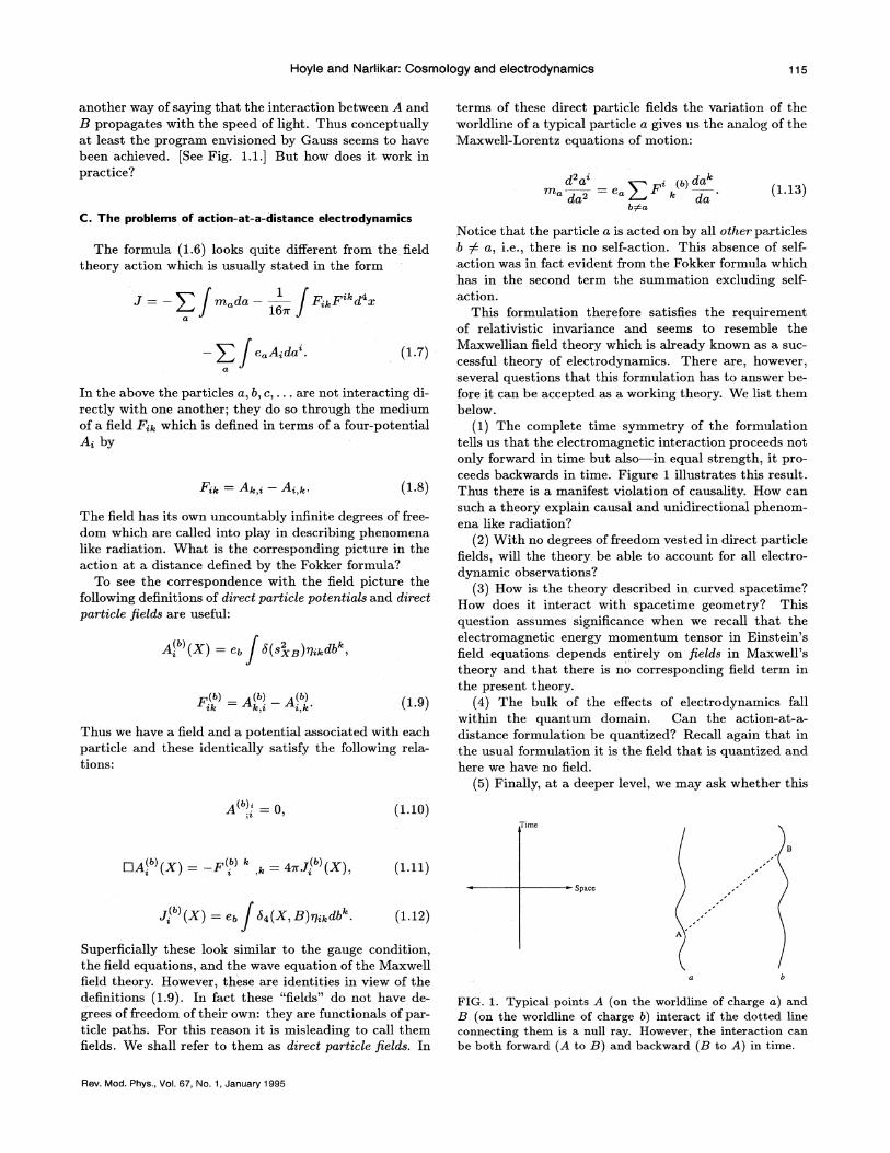
(1) The complete time symmetry of the formulationtells us that the electromagnetic interaction proceeds notonly forward in time but also—in equal strength, it pro-ceeds backwards in time. Figure 1 illustrates this result.Thus there is a manifest violation of causality. How cansuch a theory explain causal and unidirectional phenom-ena like radiation?
(2) With no degrees of freedom vested in direct particlefields, will the theory be able to account for all electro-dynamic observations' ?
(3) How is the theory described in curved spacetime'?How does it interact with spacetime geometry'? Thisquestion assumes significance when we recall that theelectromagnetic energy momentum tensor in Einstein'sfield equations depends entirely on fields in Maxwell'stheory and that there is no corresponding field term inthe present theory.
(4) The bulk of the effects of electrodynamics fallwithin the quantuxn domain. Can the action-at-a-distance formulation be quantized? Recall again that inthe usual forInulation it is the Geld that is quantized andhere we have no field.
(5) Finally, at a deeper level, we may ask whether this
TimeJi
J{)(X) = es h4(X, B)rl, i,db". (1.12)
= Space
r
rr
rrrrrr
rr
r
FIG. 1. Typical points A {on the worldline of charge a) andB {on the worldline of charge b) interact if the dotted lineconnecting them is a null ray. However, the interaction canbe both forward {A to B) and backward {Bto A) in time.
Superficially these look similar to the gauge condition,the field equations, and the wave equation of the Maxwellfield theory. However, these are identities in view of thedefinitions (1.9). In fact these "fields" do not have de-grees of freedom of their own: they are functionals of par-ticle paths. For this reason it is misleading to call themfields. We shall refer to them as direct particle fields In.Rev. Mod. Phys. , Vol. 67, No. 1, January 1995
Hoyle and Narlikar: Cosmology and electrodynamics
II. THE ABSORBER THEORY OF RADIATION
A. The plablems of classical field thealy
The issues raised above vis a vis action at a distancecan be better appreciated against the background. of theproblexns faced by the classical field theory of Maxwell.We itemize them below although they happen to be in-terrelated.
1. Explanation of causality
The wave equation satisfied by the four-potential A;in the Maxwell theory is similar to the relation (1.11)except that in this case it is a genuine equation ratherthan an identity:
A, =4+1;. (2.1)
Here the right-hand side is the current density four-vector. In terms of our direct particle definition (1.12) itis the sum of all such four vectors.
In solving any problem in Beld theory involving theabove equation, it is common practice to choose thosesolutions of Eq. (2.1) that are consistent w'ith the prin-ciple of causality. The most fundamental problem is theone referred to by Gauss (1867), viz. that of the accel-erated electric charge. It is well known that the waveequation (2.1) has two independent basic solutions, onehaving support on the future light cone (the so-calledretarded solution) and the other having support on the
new formulation fares better than the standard field the-ory.
These challenges have been addressed by various work-ers over a span of several decades. In this review we willsummarize the progress in light of the above questions.We begin with the seminal work of Wheeler and Feynmanfirst reported in this journal nearly Bfty years ago.
past light cone (the advanced solution). Symbolically we
will denote these solutions by A,' and A, , respec-
tively, for the potentials and by I",k' and I",.& for thecorresponding fields.
Now in the problem of the accelerated charge, it iscustomary to select the retarded solution to describe thephysical situation. The advanced solution is rejected onthe grounds of causality. Thus it is argued that it isphysically realistic to have the charge radiating electro-magnetic waves which travel outwards from it and reach adistant point at a later instant; and the retarded solutiondescribes this situation. The advanced solution describ-ing waves converging from infinity onto the source chargeand crossing a distant point before they reach the sourceis manifestly unrealistic. Hence the retarded solution isthe reasonable one.
While this procedure is entirely consistent with physi-cal reality, at a deeper level it is incomplete; for it doesnot take us any further towards understanding why theprinciple of causality should operate. Expressed in asomewhat diKerent form, the phenomenon of radiationby the accelerated electric charge is a unidirectional onein terms of time whereas the basic Maxwell equationsare time symmetric. The question therefore is, why dowe have an electrodynamic arrow of timeF Field theorydoes not oKer any answer. It stops at providing a scenarioconsistent with causality. The choice of the retarded so-lution is imposed ad hoc rather than deduced.
2. Radiation damping
As a result of the choice of the retarded solution andthe phenomenon of radiation by the accelerated charge,the charge loses energy and its motion is damped. Itis possible to compute the damping force on the chargeby using the law of conservation of energy and momen-tum. In the notation of the preceding section, the equa-tion of motion of a typical charge a is modified from theMaxwell-Lorentz form to the following:
(2 2)
The F'& term here denotes the external fietd acting
on the charge. The extra term on the right-hand side isthe damping force. Notice that it has not been deducedfrom the basic field theory action whose Lagrangian onlygives the Lorentz force. It has been put in from therequirement of energy loss by radiation. For example, ifwe had chosen a time-symmetric solution, i.e. , a solutionwith half the advanced plus half the retarded fields thenthere would be no emission of radiation and no damping.
In a highly perceptive discussion of the problem Dirac(1938b) had provided a new modus operandi for the com-putation of the force of radiative damping. His prescrip-
+(a)i ~ +(a) ret i +(a) adv iIc 2 k (2.3)
Here B 'k is evaluated at the electric charge a. Al-
though both the advanced and retarded fields due to themotion of a diverge on the worldline of a, their difFerenceis Bnite and as shown by Dirac, its force on the charge isexactly equal to the extra term in Eq. (2.2). Thus the
tion was as follows. To the field I"'A, used in computing
the I orentz force in Eq. (2.2) add an extra field
Rev. Mod. Phys. , Vol. 67, No. 1, January 1995
Hoyle and Narlikar: Cosmology and electrodynamics 117
m = e E'@+Ada2 da
(2.4)
with the second term apparently arising from the chargeitself.
The Dirac prescription despite its elegance was some-what mystifying, however, in that it brought in the ad-vanced solution that had been discarded as unphysical.Dirac sought to relate its presence to another outstand-ing problem of field theory, namely the problem of infiniteself-action. We will consider it next.
3. The paradox of self-action
motion of an electric charge a is given by the modifiedequations:
ical solutions. In one we have causality but infiniteself-energy while in the other the motions are finite butacausal. Not surprisingly, it was believed that the prob-lem of self-force of the charge would not be solved exceptby recourse to quantum theory.
This hope has not been fully realized. Quantum fieldtheory does alleviate the self-energy problem but can-not surmount it without introducing the renormalizationprogram. We shall consider the quantum problem in Sec.IV. For the present we will confine ourselves to the clas-sical electrodynamics.
These comments therefore underscore the fact thatthere are conceptual problems with the classical field the-ory, and thus provide further motivation for looking atthe alternative offered by action at a distance.
Dirac (1938b) highlighted the problem with the helpof an idealized situation. Imagine an electric charge a atrest and under the action of no forces until it is hit by ahammer. The hit is thus an impulsive force which sets thecharge in motion. What happens to the charge thereafterwhen it finds itself once again under no external forces?
There are two possible solutions for describing the mo-tion of the charge. The first solution has the charge mov-
ing with a uniform velocity that it acquired as a resultof the hit. The second solution is more peculiar anddescribes the charge moving with a momentum that in-creases exponentially with time, and according to the fullrelativistic treatment given by Dirac its velocity rapidlyapproaches the speed of light. This happens because ofthe self-action force introduced in Eq. (2.4).
Although the first solution appears reasonable, it isthe second that matches the prescribed initial conditions.Under the circumstances Dirac reexamined the initialconditions and argued that they need to be altered ifthe first solution is to apply. The new situation has thecharge moving from rest at infinite past and attaining thefinal velocity just before being hit; a velocity it maintainsthereafter.
The crucial mathematical point to appreciate here isthat, with the self-action included, the differential equa-tion of motion is of third rather than second order. Thus,after an impulsive force the acceleration rather than thevelocity changes discontinuously. Physically, however,the new situation seems acausal, for the charge accel-erates in anticipation of the hit in such a way that itbuilds up the right velocity just before being hit by thehammer.
This acausal behavior of the charge can be rationalizedby pointing out that the self-action force as computedby Dirac's method does include the advanced field. Inpractical terms the duration of acausality is of the ordere /m c which is not only very small but also is small bythe factor 1/137 compared to the Compton time scale as-sociated with the charge (assuming that it is an electronor a proton).
The above discussion (see also Hoyle and Narlikar,1993 for details) offers us a choice between two unphys-
B. The Wheeler-Feynman approach
Fifty years ago, Wheeler and Feynman (1945) ad-dressed the above issues in an attempt to revivethe action-at-a-distance formulation as derived bySchwarzschild, Tetrode, and Fokker (see references in theprevious section). The central themes of their argumentwere that an action-at-a-distance theory was necessarilynonlocal and that the apparent acausality in its resultsarose from inadequate attention being paid to the inter-action of a typical charge a with all the other charges inthe universe, even if they happen to be located far away.
1. A simple illustrative example
(2.5)
To simplify the picture further, Wheeler and Feynman as-suined the local region around the charge o, to be empty,in the form of a spherical cavity centered at r = 0, andextending as far as r = Band the universe beyond havingN charges per unit volume.
In vacuum the full retarded electric field of the chargea at a point P located at a large distance r from it wouldbe given by
eEs = u —sinoexp [iu(r —t)] (2 6)
To illustrate how the distant charges influence a localexperiment we will repeat briefly the simple derivationgiven by Wheeler and Feynman in their above-mentionedpaper.
We assume the universe to be static, Euclidean, witha uniform number density of charges e and with the lineelement of special relativity as given in Eq. (1.3). Letthe charge a be located near the origin 0 of sphericalpolar coordinates (r, 8, P) and suppose that its motionthere is Fourier analyzed with a typical component ofthe acceleration given by
Rev. Mod. Phys. , Vol. 67, No. 1, January 1995
118 Hoyle and Narlikar: Cosmology and electrodynamics
in the direction of increasing 0 where 0 is the angle madeby the direction OP with that of the acceleration vectoru . We have taken c = 1.
This result, however, needs to be modiBed to includethe refraction eKect at the boundary r = B of the cavityand the phase change due to the refractive index n —ikof the medium beyond. The latter is related to the eKectthe basic Beld produces on the motion of a typical chargeat P. Thus, we modify (2.6) to
2eu sin 0Es = . exp [i~(r —t+ (n —ik —l)(r —R) j],r(1+ n —ik)
(2.7)and use the field Eg to compute the acceleration of thecharge at P. This is given in the direction of Eg by
universe. Multiplying this field by the charge gives usthe standard formula for the radiative damping force
2eRe = a.
3(2.13)
y (a)ret ~(a)adv2
It can be verified that this is the nonrelativistic versionof the Dirac term in Eq. (2.2).
If instead of calculating the sum of responses at thelocation of a we had calculated it at an arbitrary pointin its neighboring region, we would have found that thefield is Dirac's extra field (2.3),
e—p(~) &s (2 8)
where p(u) is a frequency-dependent function, deter-mined in terms of the refractive index by the formula
e eEs p(w) —s—in 0 exp ( icur)—
m 2r(2.1O)
The net response of all such particles along the futurelight cone of a is given by the integral
OO & 27K
p((u) si One' "Es Nr
=R 8=0 y 0 2m'xsin8 drd0dg
2 —2'W 4——zueu e3
(2.11)
The responses normal to the acceleration vector cancelout and so we may use Eq. (2.11) to sum over all fre-
quencies and arrive at the result
2e. ..R = —a.3
(2.12)
This is the field that the charge a itself would experiencebecause of its action at a distance with the rest of the
4' Ne2(n —ik) = 1 — p(cu).m+2
The crucial step in the Wheeler-Feynman theory was torecognize that in the action-at-a-distance formulation themotion of the particle at P will generate a reaction whichwill arrive at a backwards in time, i.e. , at the instant thatthe original retarded field left it. This reaction is the halfadvanced Beld of the particle at P. Further, to study theelectrodynamics in the vicinity of a we must evaluatesuch responses from all particles lying on the future lightcone of a.
The half advanced electric field at a due to the sourceacceleration at P as given by Eq. (2.6) when resolved inthe direction of the acceleration of a then becomes
This calculation is slightly more involved and may befound in the work of Wheeler and Feynman (1945). Usingthis result, they built up a self-consistent picture of actionat a distance in the following way.
In the above calculation the net field emanating fromcharge n is the full retarded field. How is it made up7 Itis made up of two components as given below:
p(a)ret p(a)ret + p(a)adv1
2
+ ~(a) ret ~(a)adv1
2(2.15)
The first term on the right-hand side is the basic time-symmetric Geld of charge a while the second term, as wejust saw, represents the response of the universe. Thecalculation is thus self-consistent since it was the full re-tarded Beld that was used in computing the response.
We therefore see that Dirac's mysterious prescriptionreceives a natural derivation in the action at a distanceframework. We also see that the radiative reaction is nota self-force but is the combined reaction of the universeto the motion of the charge a. Further, even though ourtheory is time symmetric, we seem to have arrived at anexplanation of why retarded solutions operate in practice:it is not an ad hoc choice required by causality but forcedon us by the way the universe responds.
It might be argued that the elegant result obtainedabove may be due to our oversimpliGed choice of param-eters describing the universe. The universe is not homo-geneous. It may consist of charged particles of variousmasses (e.g. , electrons and protons). The cavity imag-ined around the charge a may not be spherical. Is theresult sensitive to these issues'
Wheeler and Feynman demonstrated that these issuesare not important. The crucial issue is that of completeabsorption. The integral in Eq. (2.11) must then con-verge to the value it has in Eq. (2.11). This is ensuredby the presence of a sufhcient number of particles to thefuture of a that can absorb the disturbance coming outfrom a and react to it. The condition may be stated thus:the universe must be a perfect absorber of all electromagnetic fields emanating from urithin. The self-consistency
Rev. Mod. Phys. , Vol. 67, No. 1, January 1995
Hoyle and Narlikar: Cosmology and electrodynamics 119
argument implied by Eq. (2.15) will not work if the uni-verse is an imperfect absorber. We will now state thisrequirement mathematically and use it to give a generalderivation of the above result.
p(b)ret p(b)adv 0b
The field acting on charge a therefore becomes
(2.19)
2. The general resulty (b)ret + y (b)adv
bga
I et us consider the universe as static and with Eu-clidean geometry. The electric charges in it are movingarbitrarily and we will denote by E( )re and P( ) theretarded and advanced Gelds of a typical charge a. Weremind the reader that the fields referred to here are di-rect particle fields and hence do not have extra degreesof freedom of their own. Thus the retarded and/or ad-vanced field implied here is well defined with respect tothe light cones future and/or past of the correspondingparticle.
We now state the property of perfect absorption as im-plied by Wheeler and Feynman (1945) as follows: Whenany arbitrary electric charge a is accelerated, all elec-tromagnetic fields arising from its motion directly orthrough its interaction with other charges —should tendto zero suKciently rapidly at great distances from a. If weconfine our attention to only such fields, then the abovecondition means
E( )" + I" ( o~ —~
as r -+ oo. (2.16).1 s,,t s d t'l1
In vacuum, a radiative field falls asymptotically as rand the more rapid fall implied by Eq. (2.16) indicatesperfect absorption. The proof given by Wheeler andFeynman that in a perfectly absorbing universe only re-tarded interactions survive is as follows.
Since in (2.16) we have a combination of incoming andoutgoing waves, for the relation to hold at all times weneed the two types of waves to vanish asymptoticallyseparately. Thus Eq. (2.16) implies two relations:
) ~(»-t2 (r)
(2.17)
) y (b)adv
r) asr Moo,
and hence also
) ~(b)ret F(»adv—"2 as r -+ oo. (2.18)
However, unlike Eq. (2.16) the above combination rep-resents a sourceless field and hence a solution of the ho-mogeneous wave equation. As such, its faster than rbehavior at infinity implies that it must vanish identicallyeverywhere. Hence
yl(»ret + y7(a)ret pl{a)adv (2 2())2
bga
The first term on the right-hand side represents the re-tarded field of all other charges b g a acting together ona while the second term is the Dirac radiative reaction.
We therefore arrive at the general version of the resultderived in the simple example considered earlier, thushighlighting the role of perfect absorption by the uni-verse. For this reason, Wheeler and Feynman called thistheory the absorber theory of radiation.
3. Enter cosmology
The apparent resolution of the causality problem in ac-tion at a distance was, however, not quite complete in itslogical framework as Wheeler and Feynman themselvespointed out. We can see the problem in the following way.In the above general argument interchange the words ad-vanced and retarded to find that the chain of reasoningstill goes through with (2.20) replaced by
) g(b) ret g(b) adv
bga
~ g(b)adv + g(a)adv g(a)ret+2bga
(2.21)
This means that the charge a is acted on by the advancedfields of all other charges and a radiative reaction that isthe exact opposite of that given by Dirac.
There is nothing to prevent us from using Eq. (2.21)instead of Eq. (2.20), but in practice it would be veryawkward. For example, in the simple example discussedearlier, we had assumed that the absorber particle wasat rest before being hit by the retarded wave from thesource. This is reflected in the first term on the right-hand side of Eq. (2.20) which is uncorrelated with themotion of a. In Eq. (2.21), on the other hand, the firstterm is highly correlated with the motion of a and hence ifwe took those correlations into account we would recoverEq. (2.20).
On the other hand, we could use Eq. (2.21) to describea new situation in which the universe admits only theadvanced solutions. The simple example of Sec. II.B.1would then have a counterpart in which the accelerationof a generates advanced, i.e., incoming waves which hitthe absorber particles before reaching the source charge.A typical absorber particle must move in such a way that
Rev. Mod. Phys. , Vol. 67, No. 1, January 1995
120 Hoyle and Narlikar: Cosmology and electrodynamics
g~(ret) + ~~(adv) (2.22)
where A. and B are constants. Now, we have seen thata full retarded solution gives the Dirac radiative reac-tion in a perfectly absorbing universe. With an absorberof efficiency f the field AF(" ) will therefore generate aradiative reaction Af times the Dirac value. Similarly,the field BI'"( ) will generate a reaction —Bp times theDirac value. For self-consistency therefore, the net radia-tive reaction (Af —Bp) times the Dirac value added tothe basic elementary field of the charge a should give usthe net field assumed in Eq. (2.22):
after the incoming wave has hit it, it comes to rest.Wheeler and Feynman argued that while a priori there
is nothing to prevent us from imagining a universe withinitial conditions set up in the above fashion, in thethermodynamic context such artificial initial conditionswould appear highly unlikely. In fact, this distinc-tion between Eqs. (2.20) and (2.21) was, according tothem, dictated by thermodynamic time asymmetry. Thetime asymmetry in electromagnetic radiation arises fromasymmetrical initial conditions that favor Eq. (2.20) overEq. (2.21), i.e. , from the time asymmetry in thermody-namics.
It turns out, however, that this recourse to thermo-dynamics is unnecessary. The crucial consideration thatbreaks the time symmetry of the action at a distancetheory comes from cosmology. This was erst pointed outby Hogarth (1962) who argued that, if due note is takenof the cosmological fact that the universe is expanding,then the symmetry between the two situations leadingto Eqs. (2.20) and (2.21) is broken. For, if we examinethe proof of the general result of Wheeler and Feynmangiven above, we notice that to prove the consistency ofretarded solutions we require perfect absorption in thefuture, and likewise we need perfect absorption in thepast for the consistency of the advanced solutions.
The early observations of Hubble (1929) based on theredshifts of the nearby galaxies and clusters have sincebeen extended to galaxies considerably farther away andthe picture of the expanding universe has come to begenerally accepted. Most cosmological models today arebased on this concept. Thus the assumption of a staticuniverse by Wheeler and Feynman was unrealistic. Hog-arth's argument can be reworded in the following way tounderscore the crucial role of cosmology in action-at-a-distance electrodynamics.
Suppose that we have a universe that has future andpast absorbers operating at different e%ciencies which weshall denote by factors f and p. Thus f = 1 denotes aperfect future absorber while p = 1 a perfect past ab-sorber. Let such a universe lead to a net self-consistentsolution of the form
Equating the coeKcients of the advanced and retardedfields in Eqs. (2.22) and (2.23) separately, we determinethe coeKcients A and B as
1 —f2 —f —p
(2.24)
C. Cosmological considerations
1. Action at a distance in curved spacetime
As discussed above we will G.rst develop the generalframework for describing the action-at-a-distance elec-trodynamics in Riemannian spacetime and then apply itto some of the standard models of the universe. Such aframework was first given by Hoyle and Narlikar (1964a)in their attempts to follow up Hogarth's lead in a morecomprehensive manner.
Thus instead of the Minkowski line element of Eq. (1.3)we have
d8 = g Idx Iz (2.25)
and the question arises, in what way can we generalize theh(s~&&) type of interaction to the above spacetime. Al-
though the square of the interval 8&& between two worldpoints A, B along the geodesic joining them (assuming itto exist and to be unique) is definable in a Riemannianspacetime, any operations of calculus on it are extremelyintricate and do not lead us to Maxwell-like equations.The correct procedure lies in the generalization of thewave equation (1.5) to curved spacetime.
Synge (1960) had developed the necessary basic frame-work which was subsequently used by Dewitt and Brehme(1961) for defining the Green's functions of the wave
equation in a Riemannian spacetime. In formulating ac-tion at a distance these Creen's functions play the basicrole of the above delta function. We will use the notationof Hoyle and Narlikar (1963) in what follows.
Accordingly we will rewrite the Fokker action (1.6) incurved spacetime in the following form:
Notice that if f = 1 we get the full retarded field asthe self-consistent answer so long as p g 1. Similarly, for
p = 1 and f g 1 we get the full advanced field as the self-consistent answer. Only for the case p = f = 1 do we runinto an ambiguous situation. This last was precisely thecase encountered by Wheeler and Feynman. Hogarth onthe other hand showed that most familiar cosmologicalmodels lead to unambiguous results.
Before we can examine the cosmological implicationsin detail, however, we have to prepare the groundworkfor describing action at a distance in curved spacetime,since cosmology uses that framework.
y (ret) + y (adv)12
(Af B ) P (ret) F(adv) (2 23)2 (2.26)
Rev. Mod. Phys. , Vol. 67, No. 1, January 1 995
Hoyle and Narlikar: Cosmology and electrodynamics 121
&A&B &B&A & (2.27)
Here the first term is a straightforward generalizationbut the second one needs some explanation. The Green'sfunction Gi„;B takes the place of the flat spacetime termh(sAB)g;k and has the following properties:
function vanishes in flat spacetime. We therefore see aconnection with the b(s2AB) term of the Fokker action.Here we briefly run through the formalism just to illus-trate how the action at a distance is describable anal-ogously to the flat spacetime version. Thus the directparticle potential and field are defined by
&xGix.-B + &;
= [—g(K, B)] ~ g;; h4(X, B) (2..28)
A( ) = 4mt. b G, i db'B,
ix I x A:x;ix ix;A:x '
(2.30)
&A&B p&A&B ( AB) + 'V&A&B ( AB) (2.29)
where p; „;B and qi„iB are two-point functions and 0 isthe Heaviside function. The latter part of the Green's
Notice first that we have attached suKxes to the ten-sor indices to indicate the spacetime point at which theyoperate. This is necessary since the property of tensorcovariance is a local one in curved spacetime. Instead offunctions of one spacetime point common in field theory,here we are forced to use quantities that are invariant orcovariant at two points where they are defined.
The relation (2.27) indicates the property of symmetrybetween the two points A, B at which Gi„;B acts as a vec-tor. It is this property that ensures time symmetry of theaction deffned above. The relation (2.28) is the identitysatisfied by the Green's function. The two-point vectoron the right-hand side is the so-called paralle/ propaga-tor introduced by Synge (1960) to describe the parallelpropagation of a vector along the geodesic joining twopoints.
For detailed properties of G;„;B see Dewitt andBrehme (1961) and Hoyle and Narlikar (1963, 1964a).For example, the Green's function has the followingstructure
and, in view of Eq. (2.28) the following relations alsohold:
(2.31)
where the current vector is de6ned as a straightforwardcurved space analog of Eq. (1.12). (Where there isno ambiguity the suffix on a tensor index is dropped. )The Lorentz force equation is likewise a generalization ofEq. (1.13) which need not be explicitly stated.
The action so formulated answers'question (3) raisedin Sec. I.C, even in relation to the effect of direct particlefield on the spacetime geometry. For a variation of themetric tensor alters the spacetime in which the Green'sfunction GiAiB is defined. As a result the Green's func-tion also changes and hence the action. It can be shownthat this variation leads to an energy momentum tensordefined in terms of direct particle fields that resemblesthe energy momentum tensor of the Maxwell field theory(Hoyle and Narlikar, 1964a).
Earlier Wheeler and Feynman (1949) had speculatedwhether the action-at-a-distance theory would producesuch a gravitational effect. Prom purely flat spacetimearguments they had arrived at two possible forms of theenergy tensor:
g(a)g(b)lm g g p(a)'ly(b)I + g(b)ily(a)kFrenkel 4 2g / ~ / ~ lm l+ l
a a(2.32)
'k ~ ~A:
Tcanonical 4'
a
~(a)adv~(b) retlm
b
g(a)adv ilg(b)ret A:
l
lm + +(b)adv+(a)ret lmlm
~(b)adv il~(a)«t A:
l (2.33)
The first one they called the FrenkeI tensor and the sec-ond the canonical tensor. They had concluded
From the standp. oint of pure electrodynamics it is not possible to choose between the twotensors The difj'erence . is of course significant for the general theory of relativity, where
energy has associated toith it a gravitationalmass. So far we have not attempted to discriminate between the two possibilities by may
of this higher standard
It was subsequently shown by Narlikar (1974) that itis the canonical tensor that arises from the above varia-
Rev. Mod. Phys. , Vol. 67, No. 1, January 1995
Hoyle and Narlikar: Cosmology and electrodynamics
tional procedure.We now leave these formal aspects of action at a dis-
tance in curved spacetime since we shall need them only
marginally. Our aim has been to demonstrate that withthe above kamework it is legitimate to talk of an ab-sorber theory in the curved spacetime of an expandinguniverse.
2. Cosmological models
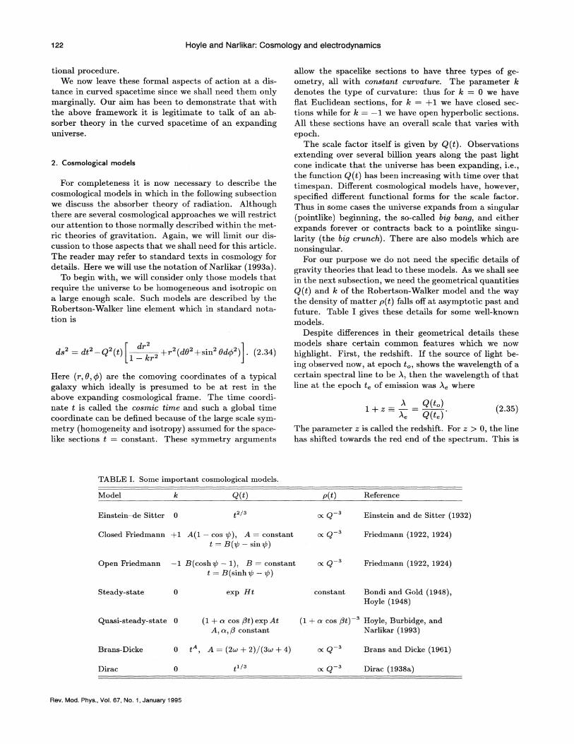
For completeness it is now necessary to describe thecosmological models in which in the following subsectionwe discuss the absorber theory of radiation. Althoughthere are several cosmological approaches we will restrictour attention to those normally described within the met-ric theories of gravitation. Again, we will limit our dis-cussion to those aspects that we shall need for this article.The reader may refer to standard texts in cosmology fordetails He.re we will use the notation of Narlikar (1993a).
To begin with, we will consider only those models thatrequire the universe to be homogeneous and isotropic ona large enough scale. Such models are described by theRobertson-Walker line element which in standard nota-tion is
2 2 2dr'
ds2 = dt2 —Q2(t) +r (do +sin Odg ) . (2.34)
Here (r, o, P) are the comoving coordinates of a typicalgalaxy which ideally is presumed to be at rest in theabove expanding cosmological frame. The time coordi-nate t is called the cosmic time and such a global timecoordinate can be defined because of the large scale sym-metry (homogeneity and isotropy) assumed for the space-like sections t = constant. These symmetry arguments
allow the spacelike sections to have three types of ge-ometry, all with constant curvature. The parameter A:
denotes the type of curvature: thus for k = 0 we haveBat Euclidean sections, for k = +1 we have closed sec-tions while for k = —I we have open hyperbolic sections.All these sections have an overall scale that varies withepoch.
The scale factor itself is given by Q(t). Observationsextending over several billion years along the past lightcone indicate that the universe has been expanding, i.e.,the function Q(t) has been increasing with time over thattimespan. Diferent cosmological models have, however,specified diferent functional forms for the scale factor.Thus in some cases the universe expands from a singular(pointlike) beginning, the so-called big bang, and eitherexpands forever or contracts back to a pointlike singu-larity (the big crunch). There are also models which arenonsingular.
For our purpose we do not need the specific details ofgravity theories that lead to these models. As we shall seein the next subsection, we need the geometrical quantitiesQ(t) and k of the Robertson-Walker model and the waythe density of matter p(t) falls off at asymptotic past andfuture. Table I gives these details for some well-knownmodels.
Despite di8'erences in their geometrical details thesemodels share certain common features which we nowhighlight. First, the redshift. If the source of light be-ing observed now, at epoch t, shows the wavelength of acertain spectral line to be A, then the wavelength of thatline at the epoch t, of emission was A, where
1+z = —= Q(t ) (2.35)A.
The parameter z is called the redshift. For z ) 0, the linehas shifted towards the red end of the spectrum. This is
TABLE I. Some important cosmological models.
Model Reference
Einstein —de Sitter 0
Closed Friedmann +1 A(l —cos @), A = constantt = B(Q —sin@)
Einstein and de Sitter (1932)
Friedmann (1922, 1924)
Open Friedmann —1 B(cosh@ —1), B = constantt = B(sinhg —vP)
Friedmann (1922, 1924)
Steady-state constant Bondi and Gold (1948),Hoyle (1948)
Quasi-steady-state 0 (1 + a cos Pt) exp AtA, o, P constant
(1+n cos Pt) Hoyle, Burbidge, andNarlikar (1993)
Brans-Dicke
Dirac
0 t, A = (2u) + 2)/(3u) + 4) Brans and Dicke (1961)
Dirac (1938a)
Rev. Mod. Phys. , Vol. 67, No. 1, January 1995
Hoyle and Narlikar: Cosmology and electrodynamics 123
invariably the case and so we conclude that observationsof all discrete extragalactic sources show that the lengthscale of the universe has increased since the time light lefta typical source. Thus in an expanding universe, lighttraveling towards the future (as in a retarded solution)is redshifted, while that traveling towards the past (as inan advanced solution) is blueshifted.
A second feature of expanding models different fromfIat spacetime is the epoch dependence of density. Asseen from Table I the density in general behaves as afunction of the epoch and thus the past absorber is phys-ically different from the future absorber. Hence, unlessone carries out explicit computations one cannot decidehow one absorber will respond based on the knowledgeof how the other does.
Thus it is clear that when discussing the interactionwith the future absorber we are dealing with low energywaves while in the case of the past absorber the inter-acting waves are of high energy. Likewise, except in thecase of the steady-state and the quasi-steady-state mod-els, and the closed Friedmann model, the future absorberhas low density and the past absorber high density ofabsorbing matter. These issues will be relevant to ourdiscussion of the absorber theory in these models.
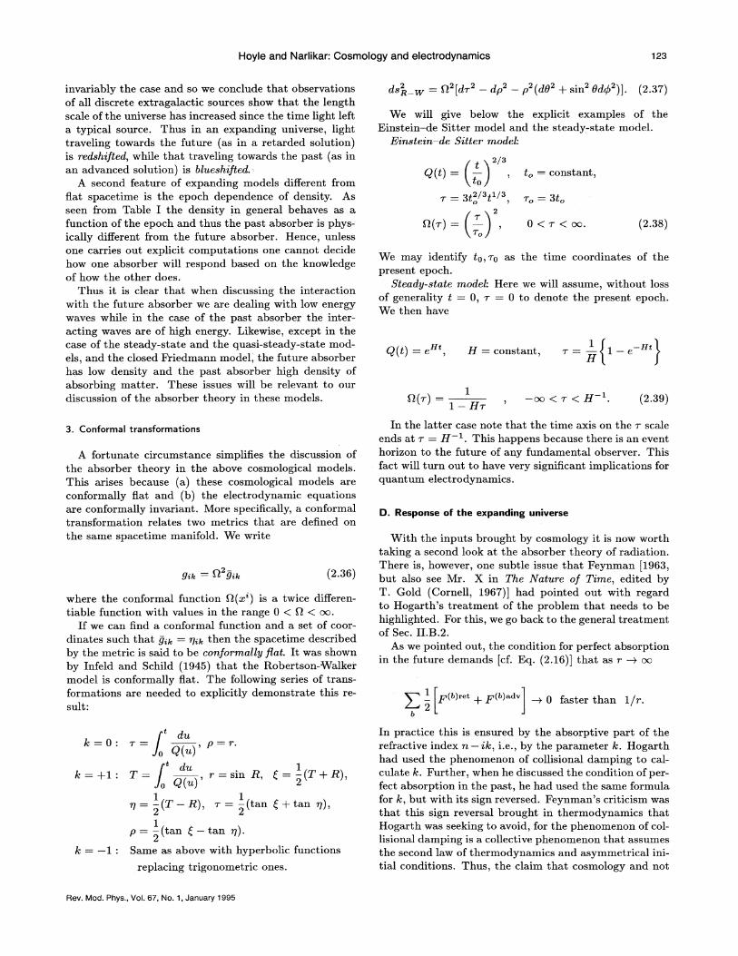
dsR ~ ——0 [dr —dp —p (d8 + sin Odg )] . (2.37)
= constant,
&O = 3&o
0&w&oo. (2.38)
We may identify t0, 70 as the time coordinates of thepresent epoch.
Steady-state model: Here we will assume, without lossof generality t = 0, v. = 0 to denote the present epoch.We then have
Q(t) = H = constant,
O(r) = 1 —oo & ~ & H (2.39)
We will give below the explicit examples of theEinstein —de Sitter model and the steady-state model.
Einstein —de Sitter model:
3. Conformal transformations
g.A:= ~~ g'k (2.36)
where the conforrnal function A(x') is a twice differen-tiable function with values in the range 0 & 0 & oo.
If we can And a conformal function and a set of coor-dinates such that g;A, ——g;I, then the spacetime describedby the metric is said to be conformally fIat. It was shown
by Infeld and Schild (1945) that the Robertson-WValker
model is conformally Bat. The following series of trans-formations are needed to explicitly demonstrate this re-sult:
A fortunate circumstance simplifies the discussion ofthe absorber theory in the above cosmological models.This arises because (a) these cosmological models areconformally flat and (b) the electrodynamic equationsare conformally invariant. More speci6cally, a conformaltransformation relates two metrics that are defined onthe same spacetime manifold. We write
In the latter case note that the time axis on the v scaleends at w = H . This happens because there is an eventhorizon to the future of any fundamental observer. Thisfact will turn out to have very significant implications forquantum electrodynamics.
D. Response of the expanding universe
With the inputs brought by cosmology it is now worthtaking a second look at the absorber theory of radiation.There is, however, one subtle issue that Feynman [1963,but also see Mr. X in The Nature of Time, edited byT. Gold (Cornell, 1967)] had pointed out with regardto Hogarth's treatment of the problem that needs to behighlighted. For this, we go back to the general treatmentof Sec. II.B.2.
As we pointed out, the condition for perfect absorptionin the future demands [cf. Eq. (2.16)] that as r + oo
) — F " + F l ~ 0 faster than 1/r2
k=0.
k=+1. T =
1 1(T —B), r = —(t—an (+tan q),
2' 2
1p = —(tan ( —tan q).
2Same as above with hyperbolic functions
replacing trigonometric ones.
In practice this is ensured by the absorptive part of therefractive index n —i k, i.e., by the parameter k. Hogarthhad used the phenomenon of collisional damping to cal-culate k. Further, when he discussed the condition of per-fect absorption in the past, he had used the same formulafor k, but with its sign reversed. Feynman s criticism wasthat this sign reversal brought in thermodynamics thatHogarth was seeking to avoid, for the phenomenon of col-lisional damping is a collective phenomenon that assumesthe second law of thermodynamics and asymmetrical ini-tial conditions. Thus, the claim that cosmology and not
Rev. Mod. Phys. , Vol. 67, No. 1, January 1995
Hoyle and Narlikar: Cosmology and electrodynamics
thermodynamics determined. the unidirectionality of elec-tromagnetic radiation was vitiated.
To get around Feynman's criticism, Hoyle and Narlikar(1963) proceeded in a difFerent way: they used the radi-ation reaction on the charge to determine the dampingparameter A:. Their approach involved first choosing aparticular combination of advanced and retarded solu-tions as the final solution and then testing it for self-consistency. Let us say that the pure retarded solutionis to be so tested. Then, given that all charges interactfinally through retarded waves, the radiation reaction isas given by Dirac [cf. Eq. (2.20)]. This reaction gives aforce of damping that, in the nonrelativistic limit, leadsto the following equation of motion for a typical absorberparticle acted on by an external electric field E:
2emr' = eE+3
(2.40)
Here e is the charge and m the mass of the particle.If we Fourier analyze with u the angular frequency of
a typical field component, then it is easy to see that therefractive index n —ik of the absorber medium is givenby the equation
In manifestly conformally Hat form this is
ds = —~
[dr —dr —r (d0 + sin Odg )]. (2.44)ro)
Let us first test for the consistency of retarded solutions.Suppose a general disturbance leaves the source at
r = G at t = tp, 7 = v, and travels along the futurelight cone. We consider a typical Fourier component ofangular frequency u of the electric field emanating fromthe accelerated source. At the source we have alreadyadjusted the conformal factor of Eq. (2.44) to be unity.Thus the frequency u measured on the t scale is the sameas that on the w scale. Since the electric field is confor-mally invariant it is convenient to work with the lineelement of Eq. (2.44) as we can take over the flat space-time solution intact in these coordinates. However, as wefound in the general treatment of Wheeler and Feynman,we need not go into specific details of the electric field butneed only verify that it does indeed fall ofF faster than1/r at large distances.
The fIat spacetime expression tells us that without theinteraction with the absorber, the field falls off as 1/r.The absorber introduces a frequency-dependent factor
4miiie' 2ie*~
)n —ik =1— 1+mes 3m ( = exp
~
+ kdr~
= exp( —I), say, (2.45)Notice that in deriving the above equation and using itfor calculating the imaginary part of the refractive indexwe have not gone beyond electrodynamics; certainly notto thermodynamics. Further, if we were testing the self-consistency of the advanced solutions we would likewiseuse Eq. (2.40) with the sign of the radiative reactionterm reversed. This would change Eq. (2.41) to
4mNe~ 2ie~~
)n —ik =1—mv jm (2.42)
This reversal of sign has no relationship to thermody-namics (as was the case with Hogarth's use of collisionaldamping), but follows logically from electrodynamics.Further, the presence of the imaginary part in the re-&active index arising from the radiative reaction termtells us that we are not dealing with a pure scatteringphenomenon.
The next step in the argument is from cosmology. Be-cause a typical wave from the source undergoes a spectralshift while traveling into the past or the future, we haveto take into account its changed frequency at the time ofits interaction with the absorber particle.
To study this eKect we will consider two explicit exam-ples from Table I. First consider the Einstein —de Sittermodel whose geometrical details were given in Eq. (2.38).We rewrite its line element in the Robertson-Walker formas
4/sd = dt —
(
—[
[dr + r (do + sin Od(j')]. (2.43)t~
r(d(r) = M 1 +—
7+(2.46)
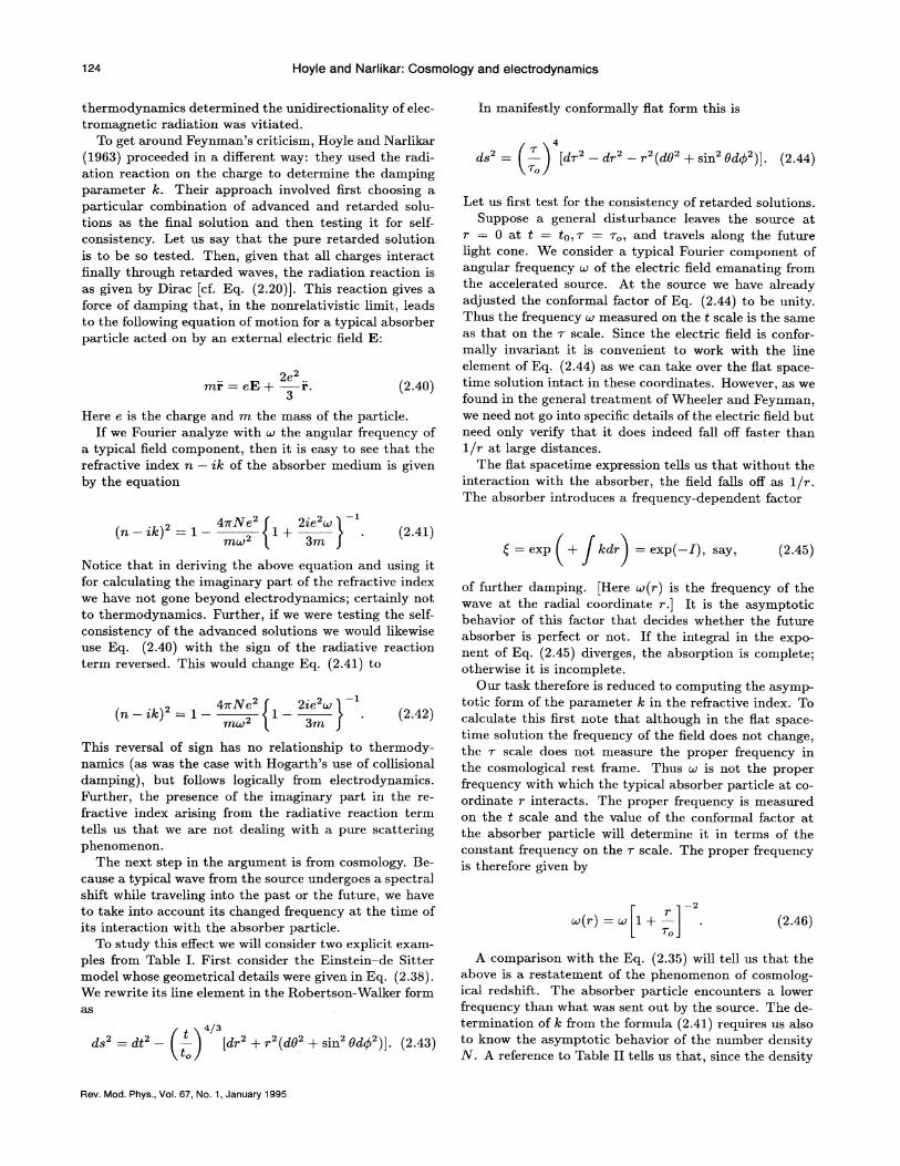
A comparison with the Eq. (2.35) will tell us that theabove is a restatement of the phenomenon of cosmolog-ical redshift. The absorber particle encounters a lowerfrequency than what was sent out by the source. The de-termination of k from the formula (2.41) requires us alsoto know the asymptotic behavior of the number density¹ A reference to Table II tells us that, since the density
of further damping. [Here w{r) is the frequency of thewave at the radial coordinate r ]It is th. e asymptoticbehavior of this factor that decides whether the futureabsorber is perfect or not. If the integral in the expo-nent of Eq. (2.45) diverges, the absorption is complete;otherwise it is incomplete.
Our task therefore is reduced to computing the asymp-totic form of the parameter A: in the refractive index. Tocalculate this first note that although in the Bat space-time solution the frequency of the field does not change,the v scale does not measure the proper frequency inthe cosmological rest frame. Thus ~ is not the properfrequency with which the typical absorber particle at co-ordinate r interacts. The proper frequency is measuredon the t scale and the value of the conformal factor atthe absorber particle will determine it in terms of theconstant frequency on the v scale. The proper frequencyis therefore given by
Rev. Mod. Phys. , Vol. 67, No. 1, January 1995
Hoyle and Narlikar: Cosmology and electrodynamics 125
TABLE II. Consistency of advanced and/or retarded solutions.
Model Future absorber Past absorber Outcome
Einstein —de Sitter
Closed Friedmann
Open Friedmann
imperfect
perfect
imperfect
perfect
perfect
perfect
advanced
ambiguous
advanced
Steady-state
Quasi-steady-state
perfect
perfect
imperfect
imperfect
retarded
retarded
Brans-Dicke
Dirac
imperfect
imperfect
perfect
perfect
advanced
advanced
p is proportional to N,
N(r) = K(0) 1+—+O
- —6
(2.47)
Using these formulas in Eq. (2.41) we find that theasymptotic value of k is given by
o, = constant (2.48)
and the integral for absorption as given in Eq. (2.45) is
OO f r tI ex~ dri1+ —
i
dr&oo.r )(2.49)
(2.50)
Note that this integral converges, thus indicating thatthe absorption is imperfect It fol. locus therefore that inthe Einstein —de Sitter cosmology, the retarded solution isnot consistent.
What about the advanced solution? We similarly con-sider the above formulas in the asymptotic limit of verylarge blueshifts. The situation at high energies is, how-
ever, not so clearcut. If we assume that interaction crosssections saturate as u -+ oo, then it can be shown [cf.Hoyle and Narlikar, 1963] that as ~ ~ oo,
We therefore have a cosmology that does distinguishbetween the past and the future absorbers, the mainpoint made by Hogarth. The final outcome, however, isthe opposite of what is found in real life. Let us now ex-amine another case from Table I, the steady-state model.
Using Eq. (2.39) it is easy to see that a retardedwave emitted at t = 0 by a source at r = 0 arrives atthe absorber particle at the coordinate r at w = r andtherefore the frequency cu at the source is redshifted tow(r) = w(1 —Hr). The number density of absorber par-ticles per unit proper volume, however, remains constantat N = No, say. Again, evaluating the parameter k in thelow frequency limit we finally get the absorption integralof Eq. (2.45) as
1 —Hr (2.52)
This integral clearly diverges, thus ensuring perfect ab-sorption in the future.
For the past absorber, a similar calculation gives theblueshifted frequency of the advanced wave at the ab-sorber particle with coordinate r to be cu(r) = w(l+ Hr).Thus again we are dealing with high frequency wavesat the asymptotic past infinity. However, the numberdensity is still constant and hence from Eq. (2.50) thelimiting value of the constant —k is oc cu(r) . So theabsorption integral of Eq. (2.45) becomes
(1+Hr) 'dr & oo. (2.53)Using the N cx u dependence and keeping in mind thefact that w is bounded below at w = 0, the integral forabsorption in the past becomes
GPI oc = +OO)0 7o P
(2.51)
i.e. , it diverges. Thus here we have the past absorberperfect and the future absorber imperfect, a situationleading to the advanced. solutions being self-consistent.
This integral converges, indicating imperfect absorption.This is another example of the past and future ab-
sorbers behaving differently. In this case, however, we doget the right answer, viz. that only the retarded solutionis self-consistent.
The calculations with regard to the response of the pastabsorber as given above carry a caveat. The determina-tion of the refractive index for very high energy wavescannot really be carried out entirely classically. Quan-
Rev. Mod. Phys. , Vol. 67, No. 1, January 1995
126 Hoyle and Narlikar: Cosmology and electrodynamics
turn efI'ects cannot be ignored. Nevertheless, as statedearlier, if the quantum cross sections converge at highenergy (as they must do) the conclusions drawn here willstand.
With regard to the models mentioned in Table I wefind a variety of answers to the above type of calculation.The results are summarized in Table II. For the cosmolog-ical models with the curvature parameter = 1 or —1 thecalculation is more involved and was carried out by Roe(1969). Davies (1972b) has also examined a whole classof cosmological models with somewhat difI'erent refrac-tive indices. His conclusions in general are similar to thatof Table II. He has, however, questioned if the trappingof redshifted waves of frequencies below the plasma fre-quency in the future absorber of the steady-state universecan be interpreted as absorption. The point, however, isthat whatever the physical process it will eventually en-sure absorption of all waves of progressively decreasingfrequencies as they travel through a future absorber ofconstant density and infinite extent. Thus the condition(2.16) is satisfied.
Davies (1973) has also pointed out that absorption willtake place by macroscopic objects at all wavelengths; i.e. ,a galaxy will absorb photons at a rate proportional tothe photon density (oc B s) and hence if R increasesslower than t ~ as in the Dirac model the time-integratedphoton absorption diverges, giving perfect absorption. Inthe Dirac model with G oc 1/t the black hole radius tendsto zero and so if all matter in galaxies, etc. , ultimatelyends in black holes the universe would not be opaque.In this sense the Dirac model in Table II is a borderlinecase.
In some cases in Table II the models give both theadvanced and retarded solutions as self-consistent. Wecall such a case ambiguous since there the cosmologicaltime asymmetry is not able to resolve the issue and we
are not better ofI' than Wheeler and Feynman workingwithin the static universe.
Can we use collisional damping to settle t;hese issues asHogarth had attempted to do? In a self-consistent pic-ture the following must hold. If retarded solutions are tobe justified, the future absorber must be perfect and thepast absorber imperfect. Now a particular cosmologicalmodel may have a perfect future absorber using colli-sional damping; but how do we judge the efIicacy of thepast absorber? Being of thermodynamic origin the na-ture of the phenomenon along the past light cone cannotbe determined unambiguously. Thus we cannot settle theissue without an extra assumption about the thermody-namic arrow of time. Hence, if we wish to work entirelywithin the framework of electrodynamics and cosmologywe have to avoid the usage of collisional damping as themeans of absorption. Once the consistency of retardedsolutions is established, however, we can use the aboveprocess to compute any actual damping.
Where there is the correct (i.e. , retarded) solutionemerging clearly we are not only better ofI' vis a visWheeler and Feynman, but we are also better ofI' com-pared to the classical field theory, because in such mod-
els we are able to link the local electrodynamic timeasymmetry to the cosmological one and are thus able todemonstrate that the choice of retarded solutions is notad hoc but forced by the universe. The analysis givenhere therefore answers the first of the questions raisedat the end of Sec. I.C. This gain is very important inrehabilitating action at a distance as a viable classicaltheory.
From Table II it is clear that cosmologies with ongo-ing creation of matter deliver the right answer, becausein their cases the future absorber has sufhcient absorb-ing matter to be perfect while the past absorber is rar-efied enough (for high frequency waves) to be imperfect.Thus, if a workable action-at-a-distance theory is to bethe decisive criterion, these theories have to be preferredto those others (like the big-bang models of Friedmann)which give wrong or ambiguous answers. Considering,however, that this verdict on cosmology is the exact op-posite to the current beliefs in the validity of big-bangmodels more has to be said in justification of action at adistance as the correct approach to electrodynamics.
In this context, the most important issues are raised inquestions 4 and 5 at the end of Sec. I.C. Can the action-at-a-distance formulation be developed at the quantumlevel and does it throw more light on issues which troublethe field theory, e.g. , the problem of self-action? We will
review the progress on these fronts next.
III. QUANTUM ELECTRODYNAMlCS-NONRELATIVISTIC PROCESS
A. The path-integral approach te quantum mechanics
1. Introduction
We have so far proceeded along classical lines. Wehave shown that the direct-particle approach to electro-magnetism works at least as well as the Maxwell Geldapproach in explaining all the classical phenomena of theinteraction of charges, and that it links with cosmologyin an interesting way. The choice of retarded potentialsis not an ad hoc choice, but is dictated by the universeat large. Moreover, the unbounded motions of chargesmoving under the self-force do not arise in this theory.
Although success in the classical domain is necessaryfor any physical theory, it; is not suKcient. Nature, aswe understand it today, is quantum in character. Inelectrodynamics, quantum theory has unearthed a vastcollection of phenomena outside the concepts of classi-cal physics. These have been explained with remark-able success by the quantized version of Maxwell's theory,although there have been conceptual and mathematicalstumbling blocks, too. Can the direct-particle theory doas well here, if not better'?
At first sight, an attempt to extend the classical direct-particle theory to include quantum phenomena seems un-likely to succeed. In Maxwell's theory we have Gelds toquantize. The degrees of freedom of these fields result inpackets of energy called "photons, " which play such an
Rev. Mod. Phys. , Vol. 67, No. 1, January 1995
Hoyle and Narlikar: Cosmology and electrodynamics 127
important part in quantum electrodynamics. We haveno analogous degrees of freedom in direct-particle fields.Thus photons do not appear to exist in the latter the-ory. The only degrees of freedom are those vested in theparticles. Can we get all the conventional quantum elec-trodynamics by a first quantization alone? If not, thetheory fails. If we can, however, the theory must be re-garded as the superior theory, because it reproduces allobservations under fewer degrees of &eedom.
Other diKculties can be anticipated concerning parti-cles and antiparticles. In classical theory all worldlinesare endless and timelike. In relativistic quantum electro-dynamics, the worldlines can go forward and backwardin time. What happens to the "identity" of a worldlineunder these circumstances? How does the rule of no self-interaction operate under such conditions?
These are some of the problems which arise when weundertake to quantize the Fokker theory. We shall pro-ceed by stages in solving them, beginning with the sim-pler nonrelativistic picture and ending with fully rela-tivistic interactions of electrons and positrons.
2. Path amplitudes
Suppose a physical system has action S. This is de-fined in terms of "paths" I' that the system can follow incoordinate space. Classical physics tells us that not all I'are permissible. In general, there is a unique path I' froma given point Pi in coordinate space to a given point P2.Writing Fo for this path, 1 o is given by the principle ofstationary action
bS = 0 for I' = I'0.
K(P2, Pq) = ) (constant) exp (iS/h),
=0, t2 & t&. (3.3)
In (3.3) the action S is computed for each path I, andthe sum is over all I' Rom Pq to P2. The constant is anormalization constant. If, as is usual, the paths form acontinuum, the sum is replaced by an integral
t2 ( t&.
where the path Fg, g, from Pi to P2 is made up of thesegment Fpg, from Pi to P and the segment 1 g, g fromP to P2. Hence
exp [iS(1'~,~, )/&] = exp [iS(1'~,~)&]exp [iS(l'QQ )/&]
(3.6)
The integral is over the continuum of paths and is morecomplicated than the Riemann or the Lebesgue integral,which are summed over sets of points. Only limitedprogress has been made toward giving a rigorous math-ematical foundation to this concept. Feynman was able,however, to obtain all required physical answers by vari-ous subtle devices. We shall draw heavily on these tech-niques. For details see Feynman and Hibbs (1965). Theconstant in (3.3) can be absorbed in the measure of 'DI .
Suppose Pq represents the spacetime point (xq, tq) andP2 the point (x2, tq) in the motion of a particle. lett2 ) ti. Any path I' &om Pq to Pq will pass throughsome intermediate point P having time coordinate t. Letthe spatial position of P be x. Since the action functionalis additive over paths, we can write
(3.5)
Earlier, we have used this mysterious prescription, andhave noted its remarkable success in classical physics. Inthe thirties Dirac (1935) suggested the interesting idea,later developed quantitatively by Feynman, that (3.1) isthe consequence of a more general principle operatingin quantum mechanics. In quantum theory the systempermits any of the paths I' from Pq to P2, but each pathhas a definite probability amplitude proportional to
The sum over all paths from P~ to P2 can be obtained bysumming all paths 1 ~~, and F~,~ and integrating overthe spatial coordinates of P. From (3.6) together with anappropriate measure for the path integral (3.4), we get
II(22 52' 21 51) f II (22 5 ' 2, 5)II2(2, t; xi 51)!Pz.
(3.7)
exp (iS/h), (3.2)
where h is Planck's constant. A11 amplitudes add, givinga total amplitude for the system that goes from Pi toP2 In the class.ical limit h ~ 0, and (3.2) oscillateswildly as we move from path to path —with the exceptionof I'0 where (3.1) holds. Paths in the neighborhood ofI'0 make a significant contribution in this limit, whereasthe contributions from other paths average out to zero.Hence the classical principle of stationary action.
Feynman carried these ideas further by introducingthe concept of the path integral. He defined the nonrel-ativistic quantum-mechanical propagator K(P2, Pq) forthe system to go from Pi to P2 by
limg+QQ & I 4 ~
T=lA„K(Q„;Q g), (3.8)
where A„ is a constant of proportionality with the dimen-sions of spatial volume. Summing over all paths gives
Together, (3.4) and (3.7) suggest an alternative way ofdefining the path amplitude. Suppose we divide F~,~,into a large number of small segments with intermediatepoints Q, (r = 1, . . . , N —1). We can define Qo ——Pqand Q~ = Pq. Over each segment (Q„q, Q„) we mayimagine S to change very slowly. We define the amplitudefor such a segment to be proportional to K(Q; Q ) ).The amplitude along the entire path is then given by theproduct
Rev. Mod. Phys. , Vol. 67, No. 1, January 1995
128 Hoyle and Narlikar: Cosmology and electrodynamics
A„K(Q; Q i)DI' = K(P2;Qiv i)K(Qiv —i; Qiv —2) .K(Q2 Qi)K(Qi Pi)d'Qiv —i
= K(P2, Pi) (3.9)
by (3.7), the integrations of d Q„being over the timesections t = t„;r = 1, . . . , % —1.
The constants A„are again absorbed in the Ineasureof I'. Because of (3.7), the definition (3.8) leads to thesame function K(P2, Pi) as before.
Sometimes we know K but not S. Then (3.8) is usefulto define a path amplitude. The original definition (3.2)is the more direct one, however. We shall use (3.8) inrelativistic path-integral theory.
l
—mx —V ldt) (3.12)
If vre substitute this in (3.4) and use (3.10), vre find that@ satisfies the differential equation
Does it satisfy the Schrodinger equation'? The answer is"yes," and we illustrate this by a simple example. For aparticle Inoving in a potential field V, we have
3. The wave functionV'2/+ V~t =ih
2 Bt(3.13)
Suppose that, instead of knowing that the particle is at(xi, ti), we only know the probability amplitude g(xi, ti)for it to be at various spatial positions xi on the timesection t = tq. We then ask, what is the probability am-plitude g(x2, t2) of finding the particle at (x2, t2)'? Thisis obtained from the vreighted mean of K(x2, t2, xi, ti),
This is the one-dimensional Schrodinger equation. Thesame argument can readily be extended to obtain thethree-dimensional Schrodinger equation.
In vievr of (3.11) and the fact that K = 0 for t2 ( ti(no propagation backward in time) (3.13) implies that Ksatisfies the equation
g(x2, t2) = K(x2, t2, xi, ti)g(x„t, )d x, .
As t2 -+ ti, @(t2) i Q(ti). T»»mp»es
(3.io) [(0/Bt2) —(ih/2m) V'2 + (i/h) V]K(x2, t2, xi, ti)= 8, (x, —x, )h(t, —t, ). (3.14)
4. Transition probability
lim K(x2, t2, xi, ti) = 83(x2 xi).t2mt1
(3.11)
The function g is the usual Schrodinger vrave function.
I et the particle be in an initial state P, (x, ti). We wishto determine the probability that it is in state Pf (x, t2)for t2 & ti. Using (3.10), the amplitude is given by
P~( 2, xt2)K( 2, xt„xti)P;( xt i)d ix2d xi
Pf(x2, t2) exp [iS(I'2i)/h]P, (xi, ti)17I2id x2d x„ (3.i5)
where the asterisk denotes complex conjugate.The transition probability from P; to Pt is given by the square of the modulus of (3.15), i.e., by
@f(x2, t2) exp [iS(I'2i)/h]P, (xi, ti)P,*. (xi, ti) exp [—iS(I'zi/h)]cg'&f (x2, t2)
x DI g] VI 2~cL xj d x2d x~d x2. (3.16)
We shall often refer to I"2~ as a conjugate path, irnply-ing that the action along I'2~ is multiplied by —i insteadof +i.5. Perturbation theory
know the behavior of a system with action So. I et thesystem be disturbed by a potential V(x, t) over the timeinterval (ti, t2). The action during this interval is there-fore
We now consider the problem of perturbation expan-sion from the path-integral point of view. Suppose we
V(x, t) dt. (3.i7)
Rev. Mod. Phys. , Vol. 67, No. 1, January 1995
Hoyle and Narlikar: Cosmology and electrodynamics 129
We now wish to determine Kv(X2, t2, xi, ti) in terms ofthe unperturbed propagator KO(x2, t2, zi, ti). We have KV(X2 t2 zi tl)
iSO(l 2i)exp
Vdt X I 2i. (3.19)
KO(x2, t2, xi, ti) = 'S.(1»)exp (3.18) Expanding the exponential involving the integral over
V, then
Kv(x„t2; x„t, ) = expiSO (I'21)
1 (./~)2
VdtI
+ . 'DI'». (3.20)
The path integral for the unity term in this expansiongives Ko. We consider the next term
~ E2
KO (x2, t2, z, t) V(x, t) KO (x, t; x„t, )d xdt.
iSO (I'21)(3.21)
(3.23)
The integral fr Vdt is over a specific path I'21, given by21a function x(t). Suppose we take a particular instant t oftime and take all paths which pass through x(t) on theirway from Pq to P2. If we sum over these paths alone, wewill get, as in the analysis leading to (3.7), the product
Ko (x2, t2; x, t) Ko (x, t; xi, ti).
If the integral over V were absent, we would simply haveobtained (3.7). But now we have to weight (3.22) with
iV(x, t)/h. —Then we have to sum over all x, to includeall paths from 1 to 2. Finally we perform the time integralto get the entire contribution:
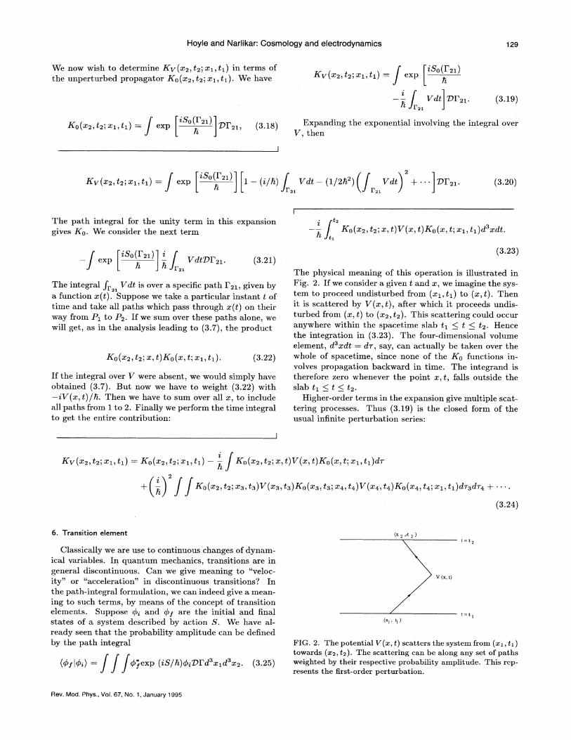
The physical meaning of this operation is illustrated inFig. 2. If we consider a given t and x, we imagine the sys-tem to proceed undisturbed from (xi, ti) to (x, t). Thenit is scattered by V(x, t), after which it proceeds undis-turbed from (x, t) to (x2, t2). This scattering could occuranywhere within the spacetime slab tq & t & tq. Hencethe integration in (3.23). The four-dimensional volumeelement, d xdt = d7, say, can actually be taken over thewhole of spacetime, since none of the Ao functions in-volves propagation backward in time. The integrand istherefore zero whenever the point x, t, falls outside theslab ti & t & t2.
Higher-order terms in the expansion give multiple scat-tering processes. Thus (3.19) is the closed form of theusual infinite perturbation series:
2KV(X2t t2i X1I tl) KO(X2t t2i X1t tl) KO(X2) t2i xi t) V(x) t)KO(zt tI xi I tl)dr
Ko(x2) t2 j x3 I t3)U(x3) 't3)K0(x3) 53I x4 it4) V(x4 I t4)K0(x4, t4j xl 'I tl)d73dT4 +
(3.24)
6. Transition element (x&,&t 2)
Classically we are use to continuous changes of dynam-ical variables. In quantum mechanics, transitions are ingeneral discontinuous. Can we give meaning to "veloc-ity" or "acceleration" in discontinuous transitions? Inthe path-integral formulation, we can indeed give a mean-ing to such terms, by means of the concept of transitionelements. Suppose P; and Py are the initial and finalstates of a system described by action S. We have al-ready seen that the probability amplitude can be definedby the path integral
/~exp (iS/h)$;VI'dsx, dsx2. (3.25)
V(x, t)
(x, , t, )
FIG. 2. The potential V(x, t) scatters the system from (xi, ti)towards (x2, t2). The scattering can be along any set of pathsfreighted by their respective probability amplitude. This rep-resents the erst-order perturbation.
Rev. Mod. Phys. , Vol. 67, No. 1, January 1995
130 Hoyle and Narlikar: Cosmology and electrodynamics
Suppose we now have a functional E[I'] of a path I'. Thenthe transition element of I' is given by
(&xl&14') = iS(I')P& exp
(61&l&*) =
As seen in this example, a transition element need notbe real even if the original dynamical variable is real.
xi[I ]y,VI d'*,d'~,
This definition means that (PylF1$;) is a certain kindof average of K[I'] over all paths suitably weighted bythe initial and final wave functions. Classically, we couldhave calculated F[I'] exactly, since we know that I' = I'o
is the unique solution. In quantum mechanics, we cannotmake such a definitive statement.
Equation (3.26) is easy to apply to simple cases. Forinstance, for a free particle of mass m, the transitionelement of velocity is given by
7. Influence functional
We come now to the concept most useful for the quan-tum development of direct-particle theories. Suppose we
have one quantum-mechanical system in interaction withanother, and suppose we are interested only in the de-tailed behavior of the Grst system regardless of what hap-pens to the second. We may speak of the second systemas the "external environment" of the Grst. To fix ideas,let the erst system be described by a coordinate q and thesecond by Q. The combined action for the two systemsis taken to be of the form
S = S,[q(t)]+ S~[q(t)]+ S,[q(t), @(t)], (3.28)
where So represents the action of the first system alone,S~ is the action of the second system alone, and SI rep-resents the interaction of the two systems. I.et P;(q;, t;)be the initial state and Py(qt, tt) the final state of thefirst system. Using (3.16), the probability of transition
P; m Pt is given by
P(P,
mph'')
= 4't(qf tf)4'*(q' t*)~'(q' t')~f(qy tt')
&«xp1
—(So[q(t)l —So[q'(t)]) I P[q q']&q&q'"qy "q'g "q'"q*' (3.29)
where
(3.30)
Here @; is the initial state of the second system. Wehave summed over all final states gt, since we are notinterested in how the environment ends up.
E[q(t), q'(t)] is called the in/uence functional and rep-resents the "force" exerted by the environment on thefirst system.
Feynman and Hibbs (1965) discuss inHuence function-als and their applications in some detail; so we shall notdiscuss them further. We expect the universe to act asthe external environment in the quantum version of theWheeler-Feynman theory. It is our aim to determine thequantum analog of the response of the universe that ear-lier we calculated classically. This response will appearin the form of an influence functional.
B. Absorption and stimulated emission
While a first quantization of particles suKces to deter-mine transition probabilities with respect to a prescribedpotential function, as in A.4 and A.5, transitions in aradiation Geld are usually considered to require a quan-tization of the Geld itself—i.e. , a resolution into photonsrather than classical wave theory. Then to match the
xP' (a', )d atd a~d a;d a,', (3.31)
where P, P are the wave functions for the states, andJ is the double path integral
S[a(t)1—S[a'(t)]k V'a(t) V'a'(t)
(3.32)
Here the path a(t) "begins" at r = a, , t = 0 and "ends"at r = at, t = T, while the path a'(t) begins at r = a', ,
t = 0 and ends at r = a&, t = T. The action S[a(t)] is a
quantization of the Geld it is usual to adopt a secondquantization of the particles. However, we shall showhere that none of this is necessary, all the standard radi-ation results being obtainable without any more quanti-zation than that given in Sec. A being needed.
In a simplified notation the probability P(m ~ n)given by (3.16) of transition in the time interval 0 (t & T from the state m to an orthogonal state n in aspecified (unquantized) external field is given by
p(m m n) = f f f 4 (ag)4 (a))JQ (a;)'„„
Rev. Mod. Phys. , Vol. 67, No. 1, January 1995
Hoyle and Narlikar: Cosmology and electrodynamics
functional of the path a(t) and is defined by
TS[a(t)] = L(a, t)dt,
0(3.33)
with the first-order term in the complex conjugate of(3.36). After a reduction that is straightforward, exceptperhaps for the calculation of the transition element ofthe velocity (Feynman and Hibbs, 1965, p. 184) one ob-tains
and similarly for S[a'(t)].We are concerned with an electronic transition and
with a situation in which
L = —ma + eV(a, t) —ea A(a, t),=1 2
2(3.34)
where e, m are the electronic charge and mass, the veloc-ity of light is taken as unity, the nonrelativistic kineticenergy is used, and V(a, t), A(a, t) are the potentials ofthe specific 6eld. In a simple one-electron atomic prob-lem the external field is made up of the electrostatic fieldwithin the atom together with the field incident on theatom. Provided the latter has no electrostatic componentit yields the vector potential A, which in the Coulombgauge satisfies
e (E„—E ) i(E„—E )t52q 5 ) o
2
x „*aa-A ad adt (3.38)
A(a, t) = /4m') (c), exp [i(k. a —kt)]
+ck exp [—i(k. a —kt)]), (3.39)
To express this result in a more familiar form expandthe incident 6eld in a Fourier series. For this step con-sider the atom as situated inside a cube with side of unitlength, the latter chosen to be very large compared withany wavelength of importance in the transition problem.Write
divA = G. (3.35)
TS)a)t)) = So)a)t)) —ej a Aett (3.36)
so that So[a(t)] is the action for the atomic field alone.Next we regard A as small enough for
~ Tie ieexp —— a Adt = 1 —— a.Adt+ . (3.37)
p p
The external field A is then wholly transverse. With thisdivision of V and A, we write
noting that k = 2'(ni, n2, ns) where ni, n2, ns are inte-gers, and that k ci, ——G because of the Coulomb gauge.Inserting (3.39) in (3.38) leads to a double sum, Pk P&,say. Waves with k g k' are regarded as coming fromdifferent oscillators and so may be regarded as being inrandom phase with respect to each other. After averag-ing gi, Pi, , thus reduces to Pi, Moreover, T is verylarge; even for allowed transitions there are a very largenumber of atomic oscillations in time T so that
Texp —(E„—E 6 hk)t dt
0
= 27rThi k + "~. (3.40)
to be rapidly convergent. The dominant term in (3.31)then involves the product of the first-order term in (3.36)
When E & E the important terms involve the minussign in the delta function, and (3.38) leads to
2 2 T 2
(4vre /h)2~
"~ ) ci, P„*(a)ae'"' P~(a)d a exp —(E„—E~ —hk)t dt
h j „" o(3.41)
where we have deferred using (3.40) until after the sum has been converted to an integral. This is the case ofabsorption.
When E & E we have the case of stimulated emission, and the corresponding result is
2 2 T 2
(4sre /5 ) ~ ~ ) ck p*(a)ae ' '
p (a)d a exp (E —E + h—k)t dt)„o (3.42)
It is not hard to see that (3.42) is the same as (3.41).Although c*e ' has replaced cI,e' the roles of thestates m, n have been switched; P is the state of lowerenergy in (3.41) whereas P is the wave function of the
lower state in (3.42). This confirms that the transitionprobability for stimulated emission in an e~ternal Beld isequal to that for absorption.
It is usual to express the transition probability in terms
Rev. Mod. Phys. , Vol. 67, No. 1, January 1995
Hoyle and Narlikar: Cosmology and electrodynamics
of the intensity of the applied field. In order to do thisit is necessary either to approximate (3.41) or to averagethe transition probability with respect to the orientationof the atom. We adopt the latter procedure. We define
Ck = Ck Rk 0'k(~) (~) (3.44)
and let n&~ i, o.&l be unit vectors which together with k/kform an orthogonal triad. Because of ck k = 0,
a „(k) = P„*(a)ae*" P (a)dsa, (3.43)
Ici, a „(k)l = Q (ci, n~'~) P„*(a)n~'l . ae*"' P (a)d a (3.45)
We have to average (3.45) with respect to orientation.It is not hard to show that the sum of
P„'(a)n„.ae*" P (a)d a. p„(a)nkvdl ae '"' p* (a)d a (3.46)
and its complex conjugate averages to zero, and that (3.45) is proportional to Ici, land can be written in the form
—Ici, l la „(k)l, where la (k)l depends on the magnitude but not the direction of k, and is equal to laI
whenthe factor exp(ik a) in (3.45) is approximated by unity. Hence the average value of (3.41) is
exp —(E —E + hk)t dt (3.47)
There are d k/(2n)s terms of this series in the elementdsk of k space. Defining Ici, I2 by
equating (3.51) to
k 3= C
d3k
we now write (3.47) in the integral form
(3.48)
dn. — I(k)dA:.kk
For this definition to hold irrespective of lckl2 we musthave
I(k) = A: Ici, I2.
exp —(E„—E —hk)t dt . d k. (3.49) Eliminating Ici, I2 between (3.49) and (3.52), and using(3.40), one easily obtains
—ExH=2) Icil kk4m
lci, l2kkd k (3.50)
and that the contribution of solid angle dO to (3.50) is
To define the intensity I(k) per unit sohd angle wenote first that dB I(k)~ia (k)~Pd~i k — "
)dk
(3.53)
for the transition per unit time. The result (3.53) appliesboth to absorption and stimulated emission, and. is theusual relation between the intensity and the transitionprobability. We can introduce separate intensities I~~i (k)for the "polarization" directions o.k by defining
lci, l2k dA:, (3.51) Il'&(k) = lci, . o. ' I2.k4 (,-)
where k lies in dO. The intensity I(k) is now defined by Evidently
Rev. Mod. Phys. , Vol. 67, No. 1, January 1995
Hoyle and Narlikar: Cosmology and electrodynamics 133
I(k) = ) IUi (k).j=l 2
(3.55)
We end the present section by introducing the conceptof opacity. Suppose there are n(k)dk atoms per unit vol-ume in state m, where E & E and (E —E )/5 liesbetween k and k+ dk. Define a mean value of Ia „(k)I2
by
&la-(k)I' n(k)dk = ).Ia-(k)l' (3.56)
Pg 4' e Pg
Ia „(k)l n(k)ds. (3.58)
Radiation traveling from Pq and P2 is reduced in inten-
sity by the factor exp[—j&' d7], it being supposed thatenough atoms are involved for the absorption probabil-ity to be averaged. It may be noted that the factorhk appears on the right-hand side of (3.57) because ofE —E = hk, not because of Geld quantization.
the summation being taken through the small volume Vfor all atoms with (E —E )/h between k and k + dk.Both Ia (k) I2 and n(k) can be functions of position aswell as of k.
Suppose radiation of frequency k travels along a three-dimensional spatial path I' connecting two points P~ andP2. Then the opacity difference between these pointsis Jr dr, where d7 is the difference for an element of thepath. To obtain &, let 8 be the three-dimensional lengthalong I' and let u(s) be the unit tangent vector at s. Theopacity differential dw(k)/ds for frequency k is defined interms of absorption by the equation
I(ku)dAdk = dOI(ku) la „(k)I2hkn(k)dk,d7. (k) 4vr e
ds 362
(3.57)
and the opacity difference is
generate spontaneous emission from the excited statesof atoms, here we have no such resource. How then isspontaneous emission to be understood and calculated' ?
To Bx ideas, let us consider the motion of particle a inthe time-interval 0 & t & T (see Fig. 3), and denote thedisplacement of a by a(t). I et b be a typical absorberparticle whose world line is intersected in intervals Aand A+, respectively, by the past and future light conesfrom the initial point [a(0), 0] and the final point [a(T), T]on the path a(t) of a. From what has been said above,the induced transitions of a arise from its interaction withthe retarded Beld of 6, i.e. , from the portion A of theworldline of 6. The action governing induced transitionsis therefore
—e A„I l (a) adt,0
(3.59)
where A„~ is the full retarded 3 potential from b. Tocalculate spontaneous transitions, we need, on the otherhand, the transitions of b induced by the full retardedBeld of a. The action governing this is
(3.60)
F[ (t) a'(t)] = F'"I (t) '(t)]e
bga(3.6i)
with a similar notation. As in the classical case, we arelooking for a self-consistent cycle of argument in whichthe net Beld is the retarded one. Throughout this calcu-lation, we shall work in a conformally Hat cosmologicalmodel with a perfect future absorber.
Our aim is to calculate the in8uence functional govern-ing the motion of a and arising from the whole universe.Since we may assume the diferent absorber particles toact independently, the inBuence functional has the form
C. Spontaneous emission
We come now to a crux in the discussion of this article,which unless it can be overcome would end the entiredevelopment. Whereas in Maxwell's theory the Beld hasindependent degrees of freedom that, after quantization,
where F[a(t), a'(t)] is the in8uence functional exerted bya typical particle b.
To calculate Fib' [a(t), a'(t)] we consider all transitionsproduced by (3.60) in the absorber particle b If g;(b) is.
the initial wave function and gf (b) any final wave func-tion of b, we have from (3.30)
~"'(~(&),a'(~)I = ) J gt(bt)gf(b'f) J~ ~g, (b;)g,*(b,')d b, d byd b', d b't, (3.62)
where
exp —(S@[b(t)] —S@[b'(t)] + SI[a(t), b(t)] —SI[a'(t), b'(t)] ) . 'Db17b'. (3.63)
With the interaction governed by (3.59), we write
Sr[a(t), b(t)] = eb A„, (b—) . bdt (3.64)
Rev. Mod. Phys. , Vol. 67, No. 1, January 1995
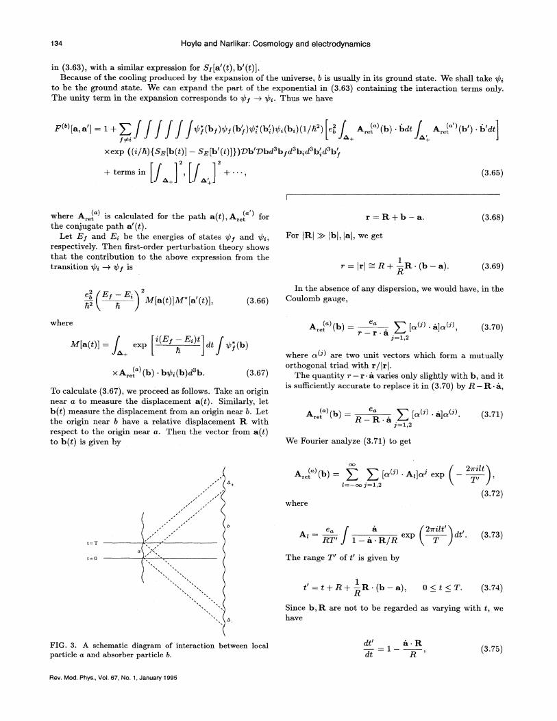
134 Hoyle and Narlikar: Cosmology and electrodynamics
in (3.63), with a similar expression for Sr[a'(t), b'(t)].Because of the cooling produced by the expansion of the universe, b is usually in its ground state. We shall take g,
to be the ground state. We can expand the part of the exponential in (3.63) containing the interaction terms only.The unity term in the expansion corresponds to gy —+ g, . Thus we have
(3.65)
r(')[a, a'] = 1+) Q~(by)gy(b't)g, *(b,')@;(b;)(1/h ) eI, A„, )(b) bdt A„, (b') b'dtfW
~I
xexp ((i/h)(S@[b(t)] —S@[b'(t)]H17b'17bd btd b;d b',.d b&- 2 - 2
+ terms in + ~ ~ ~
I
where A„I is calculated for the path a(t), A„I forthe conjugate path a'(t).
Let Et and E; be the energies of states gy and g;,respectively. Then first-order perturbation theory showsthat the contribution to the above expression from thetransltlon tP~ M (/)y 1s'
r =R+b —a.
»r IRI » lbl, lal, we g«
1r = lrl = R+ —R (b —a).R
(3.68)
'I
M[a(t)]M*[a'(t)]52( h )(3.66)
In the absence of any dispersion, we would have, in theCoulomb gauge,
M(a(t)] = j exp'
dt @~(b)i(Ey —E;)t
x A„( ) (b) . bg, (b) d b. (3.67)
To calculate (3.67), we proceed as follows. Take an originnear a to measure the displacement a(t). Similarly, letb(t) measure the displacement from an origin near 6. Letthe origin near b have a relative displacement K withrespect to the origin near a. Then the vector from a(t)to b(t) is given by
) [~(i) . a]~(i)r —r a i=1 2
where o.~~~ are two unit vectors which form a mutuallyorthogonal triad with r/lrl.
The quantity r —r a varies only slightly with b, and itis sufBciently accurate to replace it in (3.70) by R —R a,
(3.71)
We Fourier analyze (3.71) to get
///
//
///// //
//
//
// /
/
///
/
Co a k'2vrilt' )l—RT' 1 —a R/R ( T )exp
l
dt'
The range T' of t' is given by
(3.73)
A„( )(b) = ) ) [o.(') AI]o~ expl
2~iltl
l=—oo j=1,2 J(3.72)
where
1t' = t+R+ —R. (b —a)R ) 0&t&T. (3.74)
Since b, K are not to be regarded. as varying with t, wehave
FIG. 3. A schematic diagram of interaction between localparticle a and absorber particle b.
dt' a. Rdt R
Rev. Mod. Phys. , Vol. 67, No. 1, January 1995
Hoyle and Narlikar: Cosmology and electrodynamics
so that changing the variable from t' to t in (3.73) gives
e 2iril( R bT
with
T' = T —R [a(T) —a(o)]R
(3.77)
2irzl 6 a Rla exp, it — dt,T' i R (3.76)
The eÃect of dispersion in the cosmological mediumis to introduce both a phase change and damping into(3.76), modifying it to
e 1 . 2irl t' R blexp —-~, + i
2 T~( R ) o
2 iril ( a. R)a exp,~
t —~
dt, (3.7s)
the phase change being expressed by y~ and the damping by 7~.We now substitute (3.72) into (3.67). We shall make use of the fact (to be shown later) that yi is a very large phase
angle, and use this to wipe out any cross products of Ar, Ai, which arise in (3.66), except those with l = —l, giving
OC) 2 T' tf' 2
(e ei, /3R T' )[(Ef —E;) /h ] ) b;y(2irl/T') e ' exp —~Et —E; —
~
dt'hq ' T')
x )j=1 2
a Rin('&. a exp (27rli/T')/ t —I
dtR ).
, (a'. Rn(~l . a' exp 2iirl/ T'~ —t~
dt, (3.7S)R )in which we have already averaged with respect to all orientations of b to remove product terms in the components ofn(il and n( l, and where b,t( &, ) is the matrix element of b exp (i ~g,
'R ] with respect to @, and vtrf. We have also
ignored variations of b over A+ in comparison with T . Expression (3.86) can be simplified further by the results
it' ( 2~hi l, , (' 2~lhlexp —
~E, —E, —,
~
dt' = 2~T'nS~
E„—E;—T') (, T'p' (3.so)
OOsin 0! = 1.
(srl —n) 2 (3.s1)
Writing
kKhk =Ef —Ei, k=
R '
(e e~k /3R h )e "~b t(k) l )
j=1,2
and using (3.80) and (3.81), we reduce (3.7S) to the form, say,
{j} —ik a+ikt gg {j} . i ik a' —ikt~~
(3.82)
(3.s3)
[1 + ~]n(k)dkR dRdA (3.84)
Since X is very small and the index is large, we canrewrite (3.84) in the form
exp [A n(k)dkR dRdA]. (3.s5)
Suppose that at a distance R in a particular solid angledB, there are n(k) dk particles per unit volume with statesf and i such that (Ef —E,)/h lies in the range k tok + dk. Writing [b;t (k) ~2 for the average of lb;t (k)
~
forall systems satisfying this requirement, the contributionto E[a, a'] from all absorbers between R and R+ dR andin dO is
4+2 e2kd7 (k) 4ir e~ k(3.86)
the damping expressed by v (k) being due to induced up-ward transitions in the absorber. Thus (3.86) followsfrom first-order perturbation theory. Remembering thatabsorber particles contribute as a product, as in (3.61'I,we next integrate the exponent of (3.85) with respect toR and with respect to k. Using (3.86), and letting w ~ ooas B ~ oo, we obtain
The function r(k) in (3.83) is just the optical depth ofthe absorbing medium at frequency k. It is not hard toshow that
Rev. Mod. Phys. , Vol. 67, No. 1, January 1995
Hoyle and Nartikar: Cosmology and electrodynamics
exp (e /4' h)dO (j) ~
)—ik a+ikidt
T
((j) I) ik a' i—ktdt (3.87)
Integrating finally with respect to A, we obtain
E[a(t), a'(t)] = exp (e /47r 5) dOj=1 2
T
((j)
)—ik a+i@ddt
k
T
((j) ~) ik a' —iA:ddt (3.88)
The subscript k has been added to o.~~~ since we are now
integrating with respect to B, and the vectors o.~~~ changeas dO changes k is a vector in dO.
The last part of the calculation is similar to the proce-dure that led to (3.38). Expand the exponential in (3.88)and retain only the first-order term in e /h. Previouslywe had
e2 Ta Adt a'. A*dt
mould still have led to (3.38), we see that provided we
replace e2 jh2 by
e2 Ta. Adt G. Adt ) (3.89)
j=1,2
in which A was a specified field. Now we have the expo-nent of (3.88). Noting that if A in (3.89) had not been areal field
and provided we write A = o.& e ' +', the presentcase is the same as the previous one. We obtain
q~„*(a)a - n~'le'" P('a)d a
2
exp (E„—E —+ Ak)t dt (3.9I)
Using (3.40), we see that E ) E is necessary to obtain a nonzero result, and that the spontaneous emissionprobability per unit time is
(e /27rh)[(E —E ) jh] dO dk Qk=1,2
(3.92)
in agreement with the usual expression.Averaging (3.92) mith respect to solid angle and using
the same notation as in (3.53) gives
x dO. (3.93)
Nom equate the contribution from dB to (3.53) to q(k)times the contribution from dB to (3.93). This gives thefollowing definition of q(k)
(3.94)
where hk = E —E„and I(k) is separated into the tmopolarizations defined in (3.55). In the usual quantumelectrodynamics (3.94) is the relation between the fieldintensity and the average number of quanta per vacuumoscillator in the frequency range k to k+ dk. Althoughquanta do not appear explicitly in the present theory, it
is interesting that we obtain the usual formulas by takingthe spontaneous transition rate as a reference standard.It follows that, if I(k) mere to have the value appropriateto a thermodynamic radiation field at temperature T,q(k) would follow Planck's lam,
q(k) =—q(k) = (3.95)1
in which the temperature scale has been chosen so thatthe Boltzmann constant is unity.
The delta function in (3.92) gives an asymmetry be-tween emission and absorption. Spontaneous transitionsare downward because we have taken the absorber par-ticles as being in their ground levels, E, & Ef fol allf. We see therefore that the asymmetry of spontaneousemission arises from the assumption of a cold universe.We shall return to this point at the end of this section.
D. The complete influence functional and the level shiftformula
The complete influence functional mas given by (3.65),of which the two terms in the last line remain to be dis-cussed:
Rev. Mod. Phys. , Vol. 67, No. 1, January 1 995
Hoyle and Narlikar: Cosmology and electrodynamics 137
—(1/2h )
—(1/2h2) SI [a'(t), b'(t)] exp (—iSO[b'(t)]/h)@;(by)@,*. (b,'. )d byd b'. l7 b'(t).
(3.96)
It will be sufhcient to work out the erst of these terms, since the second can then be written down by inspection.Inserting (3.72) for A„I in the expression (3.64) for SI leads to
—(e /2h) )L=—ao
(A b)—27I'2lt /T dt's
(A,*.b)e "y dt'exp (iSo[b(t)]/h)Q, *(by)g, (b, )d byd b, 'D b(t). (3.97)
Using ordinary perturbation methods for second-order transitions, (3.97) can be reduced to
-("/h') ) ):[(E.-E,)jh]'l=—oo g
2 T'
vP,*. (b)(b AI)egg(b)d b exp
] [E, —E—s —( 2vrl h/T')]t' )dt'0
t'
exp)
—[Eo —E; + (2vrlh/T')]t' (dt', (3.98)
where the summation with respect to g is over all intermediate states of b.Now insert (3.78) for Ai in (3.98), to give
Eg —E; 5("/3h'~'T") ) ~
' „'~ ) [b,, (2 1/T')~"-. ( 2~hi l,
exp (i/h)~
E, —Eg — ~t' dt'T' )
exp (i/h) ~ Eg —E;+ 27rhl/T' ~t' dt' 5i
a. Rln~~i a exp —(2~ii/ T')~
t —~
dtR )
n ~ a exp (2vril/T')~
t —~
dt( a K&
B
(3.99)
after averaging with respect to the orientation of b.Although (3.99) appears complicated we shall find simplifications. For fixed @~, the main contributions come from
27r/h/T = E; —Eg. Only when this condition is satisfied can the integrals in the second line of (3.99) yield acontribution that behaves as T' . Defining
we can therefore write
E; —Eg RB' (3.1oo)
, , „) ~'~b, ,(y)~' e—.i"& —ikt' dgI
Furthermore
x )j=1 2
n{j~ . ae-ik'dtT OO
{y) ~~ik ad 2mij]!exp, (t —t —t'+t') . (3.101)
exp (t —t t'+ t') = T'b(t —t t'+ t'). — —Tl (3.1O2)
Rev. Mod. Phys. , Vo[. 67, No. 1, January 1995
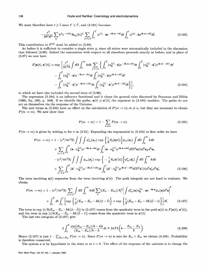
138 Hoyle and Narlikar: Cosmology and electrodynamics
We must therefore have t ) t since t' & t', and (3.101) becomes
2
, , ) k2e- (")~b,,(k)[' )g j=l,2
T t(j) ~ —ik a—iI td~ (~)
0(3.103)
This contribution to F( ) must be added to (3.88).As before it is suKcient to consider a single state g, since all states were automatically included in the discussion
that followed (3.88). Indeed the summation with respect to all absorbers proceeds exactly as before, and in place of(3.87) we now have
2
F[a(t), a'(t)] = exp dO4~'I kdk+ I (' ') "+ *'d't*
k ((j) i) ik ii' —ittt'dtlk
T(
(j))
—ik a—ietdtk
T
((j) () —ik ~'+ivtdtk
t
((j) ~
)ik a+iktdt
k
t
((j) ~ I) ik a' vktdt— (3.104)
in which we have also included the second term of (3.96).The expression (3.104) is an influence functional and it obeys the general rules discussed by Feynman and Hibbs
[1965, Eq. (99), p. 348]. If we identify the paths, a(t)—:a'(t), the exponent in (3.104) vanishes. The paths do notact on themselves via the response of the Universe.
The new terms in (3.104) have no effect on the calculation of P(m ~ n), m P n, but they are necessary to obtainP(m m m). We now show that
P(~~m) =1 —) (3.105)
P(m ~ m) is given by writing m for n in (3.31). Expanding the exponential in (3.104) to first order we have
P(m -+ m) = 1 —(e /4vr h) t('' (ag) exp So[a(t)] Ii—(a;) dn
x ) ( (j)) —ik m —iktdtk (a n„'))e*"' +'"'dt17 a(t)d a d a;
—(e'/4vr'h) &-(~', ) ~xv (—-„~0[~'(&)[)0' (~l)
j=l 2
T(~)) —ik~'+.ktdt (
~ ~ (2)) ikm' iktdt~s 1—(t)ds I ds )k k f 'c (3.106)
The term involving a(t) separates from the term involving a (t). The path integrals are not hard to evaluate. Weobtain
P(m —i m) = 1 —(e /47r h) )j=1 2
dO kdk P [(E„—E )/h] P* (a)a„') ae '" (t)„(a)d a
exp —(E —E„—hk) (t —t) + exp —(E —E„—hk) (t —t) dt.
The term in exp (i/h(E —E„—hk) (t —t) j in (3.107) comes from the quadratic term in the path a(t) in F[a(t), a (t)],and the term in exp [i/h(E —E —hk)(t —t)] comes from the quadratic term in a'(t).
The last two integrals of (3.107) give
sin[(E —E )/h —k]t ( E —E„')(E -E„)/h-k q h
(3.108)
Hence (3.107) is just 1 —P& && P(m -+ n) Since P(m ~. n) is zero for E ) E we obtain (3.105). Probabilityis therefore conserved.
The system a is by hypothesis in the state m at t = 0. The eKect of the response of the universe is to change the
Rev. Mod. Phys. , Vol. 67, No. 1, January 1995
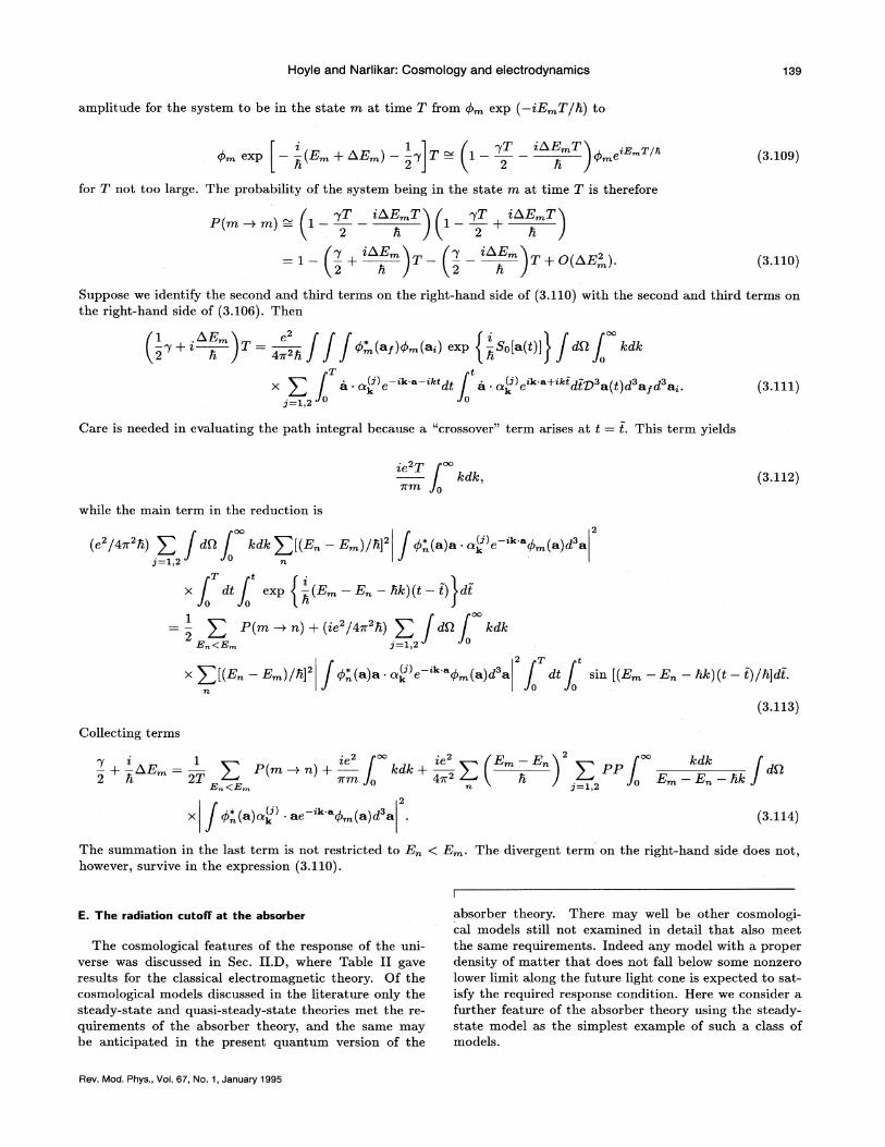
Hoyle and Narlikar: Cosmology and electrodynamics 139
amplitude for the system to be in the state m at time T from P exp (—iE T/h) to
(3.109)
for T not too large. The probability of the system being in the state m at time T is therefore
iT+ 0(b,E' ).
f pT iAE T) ( pT iAE T']Pm-+m = i1 — — 1—n )( 2 n )
iAE ) fpE2
(3.110)
Suppose we identify the second and third terms on the right-hand side of (3.110) with the second and third terms onthe right-hand side of (3.106). Then
—p+i ]T= fff 4' (at)tt (a) exp (—Ee]a(t)])f dB
Ta o,' e '"' '" dt a. o. e' ' +'" dt's a&t&~d a d a .k k af
3=12 ' 0(3.111)
Care is needed in evaluating the path integral because a "crossover" term arises at t = t. This term yields
while the main term in the reduction is
f kdk, (3.11~)
OO 2
(e /4x k) ) f dBf kdk) ](E„—E )/k] 4„'(a)a. ax e*'"'
4 (a)d a2=1,2 n
T tx dt exp (E —E —kk)—(t —t))dt
0 0
) P(m -ex)+ (te*/4x'4) ) fdBf kdk0
g —1)22 T t
P*(a)a. az(le ' '
P (a)d a Ch sin [(E —E„—hk)(t —t)/hjdt.0 0
(3.113)
Collecting terms
OO
2 h 2T—+ ~E = ) I(m~n)+ ~dk+, ) i
- "i ) ~PVlm 0 47r'
kdk
E —E„—hk
x * aok -ae ' ' ada (3.114)
I
The summation in the last term is not restricted to E ( E . The divergent term on the right-hand side does not,however, survive in the expression (3.110).
E. The radiation cutofF at the absorber
The cosmological features of the response of the uni-verse was discussed in Sec. II.D, where Table II gaveresults for the classical electromagnetic theory. Of thecosmological models discussed in the literature only thesteady-state and quasi-steady-state theories raet the re-quirements of the absorber theory, and the same maybe anticipated in the present quantum version of the
absorber theory. There may well be other cosmologi-cal models still not examined in detail that also meetthe same requirements. Indeed any model with a properdensity of matter that does not fall below some nonzerolower limit along the future light cone is expected to sat-isfy the required response condition. Here we consider afurther feature of the absorber theory using the steady-state model as the simplest example of such a class ofmodels.
Rev. Mod. Phys. , Vol. 67, No. 1, January 1995
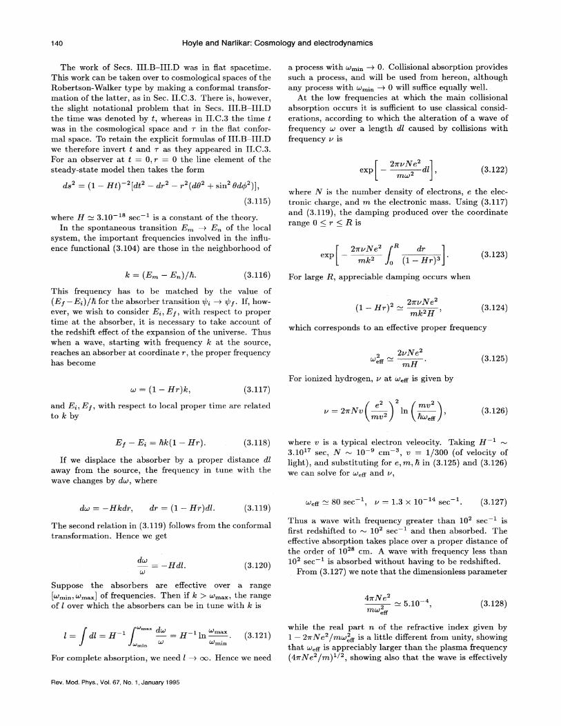
140 Hoyle and Narlikar: Cosmology and electrodynamics
The work of Secs. III.B—III.D was in Bat spacetime.This work can be taken over to cosmological spaces of theRobertson-Walker type by making a conformal transfor-mation of the latter, as in Sec. II.C.3. There is, however,the slight notational problem that in Secs. III.B—III.Dthe time was denoted by t, whereas in II.C.3 the time twas in the cosmological space and 7 in the fIat confor-mal space. To retain the explicit formulas of III.B—III.Dwe therefore invert t and T as they appeared in II.C.3.For an observer at t = O, r = 0 the line element of thesteady-state model then takes the form
ds = (1 —Ht) [dt —dr —r (dg + sin 9dg )],
(3.115)
where H 3.10 sec is a constant of the theory.In the spontaneous transition E ~ E of the local
system, the important frequencies involved in the infIu-ence functional (3.104) are those in the neighborhood of
exp2mvNe2
m(d 2 (3.122)
where K is the number density of electrons, e the elec-tronic charge, and m the electronic mass. Using (3.117)and (3.119), the damping produced over the coordinaterange 0 & r & B is
2~vNe2(3.123)
a process with ~;„~0. Collisional absorption providessuch a process, and will be used from hereon, althoughany process with ~;„m 0 will suKce equally well.
At the low frequencies at which the main collisionalabsorption occurs it is sufFicient to use classical consid-erations, according to which the alteration of a wave offrequency w over a length dl caused by collisions with&equency v is
k = (E —E„)/h.
This frequency has to be matched by the value of(Ef —E;)/h for the absorber transition Q, —+ gf. If, how-
ever, we wish to consider E, , Ef, with respect to propertime at the absorber, it is necessary to take account ofthe redshift effect of the expansion of the universe. Thuswhen a wave, starting with frequency A: at the source,reaches an absorber at coordinate r, the proper frequencyhas become
For large B, appreciable damping occurs when
2m v&e2
mI 2~ (3.124)
2vNe2efF— (3.125)
which corresponds to an efI'ective proper &equency
~ = (1 —Hr)k, (3.117)For ionized hydrogen, v at cu,g is given by
and E, , Ef, with respect to local proper time are relatedto A:by
( e' )' /mv'lv = 2vr&vi
iln
i
i mv2 ) (bc',s )(3.126)
Ef —E; = hk(1 —Hr).
If we displace the absorber by a proper distance dl
away &om the source, the frequency in tune with thewave changes by dw, where
where v is a typical electron veleocity. Taking H3.10 ~ sec, W 10 9 cm s, v = 1/300 (of velocity oflight), and substituting for e, m, 5 in (3.125) and (3.126)we can solve for ~,g and v,
dr = (1 —Hr)dl (3.119)80sec, v=13x10 sec (3.127)
The second relation in (3.119) follows from the conformaltransformation. Hence we get
(3.120)
Thus a wave with frequency greater than 102 sec —1 iserst redshifted to ~ 10 sec and then absorbed. TheefI'ective absorption takes place over a proper distance ofthe order of 10 cm. A wave with frequency less than10 sec is absorbed without having to be redshifted.
From (3.127) we note that the dimensionless parameter
Suppose the absorb ers are efI'ective over a range[w,„,cu „] of frequencies. Then if k )w, the rangeof / over which the absorbers can be in tune with k is
4' Ne25.10
mQJ g(3.12S)
&max
dl=H~min
= H ln . (3.121)~min
For complete absorption, we need l ~ chic. Hence we need
while the real part n of the refractive index given by1 —27r&e /mw, & is a little different from unity, showingthat cu ~ is appreciably larger than the plasma frequency(4vrNe /m) ~2, showing also that the @rave is effectively
Rev. Mod. Phys. , Vol. 67, No. 1, January 1995
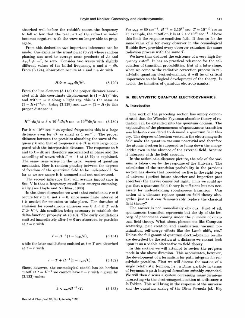
Hoyle and Narlikar: Cosmology and electrodynamics
Hdr = (u, sd k/ k. (3.129)
absorbed well before the redshift causes the frequencyto fall so low that the real part of the refractive indexbecomes negative, with the wave no longer able to prop-agate.
From this deduction two important inferences can bemade. One explains the situation at (3.79) where randomphasing was used to average cross products of A~ andA~, l g —l', to zero. Consider two waves with slightlydifferent values of the initial frequency, k and k + dk.From (3.124), absorption occurs at r and r + dr with
For w, g ——80 sec, H = 3.10 sec, T = 10 sec asan example, the cutoff on k is at 2.4 x 10 sec . Abovethis limit the response condition fails. It does so for thesame value of k for every observer in the cosmologicalHubble fI.ow, provided every observer examines the sam,radiation process with the same T.
We have thus deduced the existence of a very high fre-quency cutofF. It has no practical relevance for the cal-culation of transition probabilities. But at a later stage,when we come to the radiative correction process in rel-ativistic quantum electrodynamics, it will be of criticalimportance to the logical development of the theory. Itavoids the infinities of quantum electrodynamics.
Prom the line element (3.115) the proper distance associ-ated with this coordinate displacement is (1 —Ht) dr,and with r = t along a light ray, this is the same as(1 —Hr) dr. Using (3.129) and ~,g = (1 —Hr)k thisproper distance is
H dk/k 3 x 10 dk/k sec 10 dk/k cm. (3.130)
r = H (1 —u),s/k), (3.131)
while the later oscillations emitted at t = T are absorbedat t=r with
r = T+ H '(1 —(u.~/k). (3.132)
Since, however, the cosmological model has an horizoncutoff at k = H we cannot have C = r with r given by(3.132) unless
k ( ~,gH '/T. (3.133)
For k 10 sec at optical frequencies this is a largedistance even for dk as small as 1 sec . The properdistance between the particles absorbing the wave of fre-quency k and that of frequency k+ dk is very large com-pared with the interparticle distance. The responses to kand to k+ dk are therefore uncorrelated in phase and thecancelling of waves with /' = —l at (3.79) is explained.The same issue arises in the usual version of quantummechanics. How is random phasing between the degreesof freedom of the quantized field to be understood? Sofar as we are aware it is assumed and not understood.
The second inference that will assume importance inSec. V is that a frequency cutoff now emerges cosmolog-ically (see Hoyle and Narlikar, 1993).
In the above discussion we wrote that emission at r = 0occurs for t 0, not t = 0, since some finite interval oft is needed for emission to take place. The duration ofemission for spontaneous emission was 0 & t & T withT && k, this condition being necessary to establish thedelta-function property at (3.40). The early oscillationsemitted immediately after t = 0 are absorbed by particlesat t=r with
IV. RELATIVISTIC QUANTUM ELECTRODYNAMICS
A. Introdoction
The work of the preceding section has amply demon-strated that the Wheeler-Feynman absorber theory of ra-diation can be extended into the quantum domain. Theexplanation of the phenomenon of spontaneous transitionwas hitherto considered to demand a quantum field the-ory. The degrees of freedom vested in the electromagneticGeld make the quantum vacuum nontrivial and thereforethe atomic electron is supposed to jump down the energyladder even in the absence of the external Geld, becauseit interacts with the Geld vacuum.
In the action-at-a-distance picture, the role of the vac-uum is taken over by the response of the Universe. Thecalculation of the transition probability in the previoussection has shown that provided we live in the right typeof universe (perfect future absorber and imperfect pastabsorber) the answer comes out right. Thus we could ar-gue that a quantum field theory is sufBcient but not nec-essary for understanding spontaneous transition. Canaction at a distance replace quantum Geld theory alto-gether just as it can demonstrably replace the classicalfield theory'?
The answer is not immediately obvious. First of all,spontaneous transition represents but the tip of the ice-berg of phenomena coming under the purview of quan-tum Geld theory. What about phenomena like Comptonscattering, pair creation and annihilation, vacuum po-larization, self-energy effects like the Lamb shift, etc. '?
Unless the full gamut of quantum electrodynamic resultsare described by the action at a distance we cannot lookupon it as a viable alternative to field theory.
In this section we will attempt to review the progressmade in the above direction. This necessitates, however,the development of a formalism for path integrals for rel-ativistic particles. First we will discuss the motion of asingle relativistic fermion, i.e., a Dirac particle in termsof Feynman's path integral formalism suitably extended.We will then discuss a system containing many fermionsinteracting via the electromagnetic action at a distance ala Fokker. This will bring in the response of the universeand the quantum analog of the Dirac formula [cf. Eq.
Rev. Mod. Phys. , Vol. 6?, No. 1, January 1995
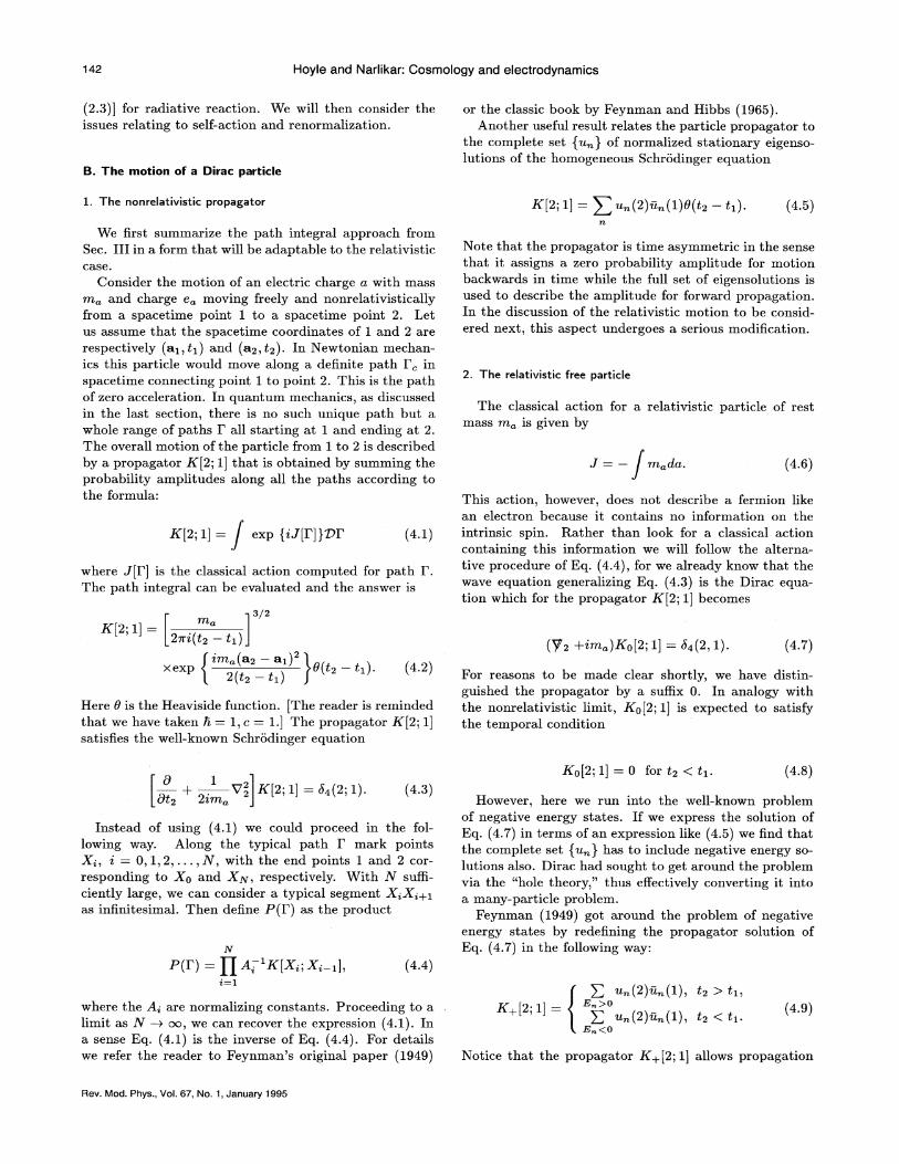
142 Hoyle and Narlikar: Cosmology and electrodynamics
(2.3)] for radiative reaction. We will then consider theissues relating to self-action and renormalization.
B. The rnotien of a Dirac particle
or the classic book by Feynman and Hibbs (1965).Another useful result relates the particle propagator to
the complete set (u ) of normalized stationary eigenso-lutions of the homogeneous Schrodinger equation
1. The nonrelativistic propagator K[2; 1] = ) u„(2)u„(1)0(t2 —t, ). (4 5)
K[2;1] = exp {iJ[1'])&I' (4 1)
where 1[I'] is the classical action computed for path I'.The path integral can be evaluated and the answer is
We first summarize the path integral approach fromSec. III in a form that will be adaptable to the relativisticcase.
Consider the motion of an electric charge a with massm and charge e moving freely and nonrelativisticallyfrom a spacetime point 1 to a spacetime point 2. I etus assume that the spacetime coordinates of 1 and 2 arerespectively (ai, ti) and (a2, t2). In Newtonian mechan-ics this particle would move along a definite path I' inspacetime connecting point 1 to point 2. This is the pathof zero acceleration. In quantum mechanics, as discussedin the last section, there is no such unique path but awhole range of paths I' all starting at 1 and ending at 2.The overall motion of the particle from 1 to 2 is describedby a propagator K[2; 1) that is obtained by summing theprobability amplitudes along all the paths according tothe formula:
2. The relativistic free particle
The classical action for a relativistic particle of restmass m is given by
J= — m da. (4.6)
This action, however, does not describe a fermion likean electron because it contains no information on theintrinsic spin. Rather than look for a classical actioncontaining this information we will follow the alterna-tive procedure of Eq. (4.4), for we already know that thewave equation generalizing Eq. (4.3) is the Dirac equa-tion which for the propagator K[2; 1] becomes
Note that the propagator is time asymmetric in the sensethat it assigns a zero probability amplitude for motionbackwards in time while the full set of eigensolutions isused to describe the amplitude for forward propagation.In the discussion of the relativistic motion to be consid-ered next, this aspect undergoes a serious modification.
K[2;1] =27ri(t2 —ti)
im. a2 —a1 'xexp 0(t2 —ti).
2(t, —t, )
Here 0 is the Heaviside function. [The reader is remindedthat we have taken 5 = 1, c = 1.] The propagator K[2; 1]satisfies the well-known Schrodinger equation
(y', +im. )Ko[2;1] = ~4(2, 1). (4 7)
For reasons to be made clear shortly, we have distin-guished the propagator by a suKx 0. In analogy withthe nonrelativistic limit, Ko[2; 1] is expected to satisfythe temporal condition
Kp[2; 1] = 0 for t2 ( ti. (4.8)
Instead of using (4.1) we could proceed in the fol-
lowing way. Along the typical path I' mark pointsX;, i = 0, 1, 2, . . . , N, with the end points 1 and 2 cor-responding to Xo and X~, respectively. With N su%-ciently large, we can consider a typical segment X,X,.+ias infinitesimal. Then define P(1) as the product
However, here we run into the well-known problemof negative energy states. If we express the solution ofEq. (4.7) in terms of an expression like (4.5) we find thatthe complete set (u ) has to include negative energy so-lutions also. Dirac had sought to get around the problemvia the "hole theory, " thus electively converting it intoa many-particle problem.
Feynman (1949) got around the problem of negativeenergy states by redefining the propagator solution ofEq. (4.7) in the following way:
P(I') = A, 'K[X;;X; i], (4.4)
where the A; are normalizing constants. Proceeding to alimit as N —+ oo, we can recover the expression (4.1). Ina sense Eq. (4.1) is the inverse of Eq. (4.4). For detailswe refer the reader to Feynman's original paper (1949)
u„(2)u„(1), t2 ) ti,K+[2;1]= &+ ' P u„(2)u„(1), t2 ( ti
E„(0(4.9)
Notice that the propagator K+[2; 1] allows propagation
Rev. Mod. Phys. , Vol. 67, No. 1, January 1995
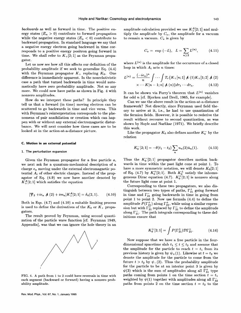
Hoyle and Narlikar: Cosmology and electrodynamics 143
backwards as well as forward in time. The positive en-ergy states (E„)0) contribute to forward propagationwhile the negative energy states (E„(0) contribute tobackward propagation. In standard language we say thata negative energy electron going backward in time cor-responds to a positive energy positron going forward intime. We shall refer to K+[2; 1] as the Feynman propa-gator.
Let us now see how all this affects our definition of theprobability amplitude if we seek to generalize Eq. (4.4)with the Feynman propagator K+ replacing Ko. Onedi8'erence is immediately apparent. In the nonrelativisticcase a path that turned backwards in time would auto-matically have zero probability amplitude. Not so anymore. We could now have paths as shown in Fig. 4 withnonzero amplitudes.
How do we interpret these paths? In principle theytell us that a forward (in time) moving electron can bescattered to go backwards in time and vice versa. Thiswith Feynman's reinterpretation corresponds to the phe-nomena of pair annihilation or creation which can hap-pen with or without any external electromagnetic distur-bance. We will next consider how these cases are to belooked at in the action-at-a-distance picture.
amplitude calculation provided we use K+ [2; 1] and mul-
tiply the amplitude by C„, the amplitude for a vacuumto remain a vacuum. C„ is given by
C = exp( —L), L=)n&2
where I & & is the amplitude for the occurrence of a closedloop in which A; acts n times:
(4.i2)
It can be shown via Furry's theorem that L~ ~ vanishesfor odd n [cf. Bjorken and Drell, 1965, for example].
Can we use the above result in the action-at-a-distanceframework'? Not directly, since Feynman used Geld the-ory to arrive at it, i.e., he had to use quantization ofthe fermion Gelds. However, it is possible to rederive theresult without recourse to second quantization, as wasshown by Hoyle and Narlikar (1971). We briefly describethis work.
Like the propagator Ko also defines another Ko by therelation
C. Motion in an external potential
1. The perturbation expansionK, [2;1] = —0(ti —t2) ) u„(2)u„(1). (4.i3)
[P2 +ie P (2) + im ]K+ [2; 1] = b4(2, 1). (4.10)
Both in Eqs. (4.7) and (4.10) a suitable limiting processis used to define the derivatives of the Ko or K+ propa-gators.
The result proved by Feynman, using second quanti-zation of the particle wave function [cf. Feynman 1949,Appendix], was that we can ignore the hole theory in an
Given the Feynman propagator for a free particle a,we next ask for a quantum-mechanical description of acharge e moving under the external electromagnetic po-tential A, of other electric charges. Instead of the prop-agator of Eq. (4.9) we now have another denoted byK++[2; 1] which satisfies the equation
Thus the Ko [2; 1] propagator describes motion back-wards in time within the past light cone at point 1. Tohave a more symmetric notation, we will denote Ko[2; 1]of Eq. (4.7) by Ko+[2; 1]. Both Ko satisfy the inhomo-geneous Dirac equation (4.7). Ko+[2; 1] is nonzero alongthe future light cone at point 1.
Corresponding to these two propagators, we also dis-tinguish between two types of paths, I && going forwardin time and I'2i going backwards in time in going frompoint 1 to point 2. Now use formula (4.4) to define theamplitude P(I'2i) along I'2i, while using a similar expres-sion but with I'2+& replaced by I'2i to deGne the amplitudealong I'2i. The path integrals corresponding to these def-initions ensure that
(4.14)
FIC. 4. A path from 1 to 2 could have reversals in time witheach segment (backward or forward) having a nonzero prob-ability amplitude.
Now suppose that we have a free particle in the four-dimensional spacetime slab ti & t & t2 and assume thatthe amplitude for the particle to reach t = ti from itsprevious history is given by g+(1). Likewise at t = t2 wedenote the amplitude for the particle to come from thefuture t ) t2 by g (2). Thus the probability amplitudefor the particle to be at an interior point 3 is given byg(3) which is the sum of amplitudes along all I'a+i typepaths coming from points 1 on the time section t = tqweighted by g(1) together with amplitudes along all I's2paths from points 2 on the time section t = t2 to the
Rev. Mod. Phys. , Vol. 67, No. 1, January 1995
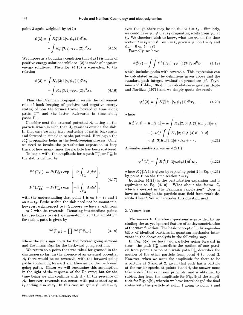
Hoyle and Narlikar: Cosmology and electrodynamics
point 3 again weighted by g(2):
g(3) = Ko [3; 1]&4/+(1)d xi
Ko [3;2]p4Q (2)d x2. (4.15)
even though there may be no Q at t = t2 . Similarly,we could have Q+ g 0 at t2 originating solely from g att2 W. e therefore wish to know, what are g+ on the timesection. t = t2 and g on t = ti given a g+ on t = ti and
= Oont=t2?Formally, we have
g(3) = K+[3; 1]p4$+(l)d x.,
K+[3;2]p4@ (2)d'x2. (4 16)
We impose as a boundary condition that g+ (1) is made ofpositive energy solutions while Q (2) is made of negativeenergy solutions. Then Eq. (4.15) is equivalent to therelation
P (12i)p4$+(1)'DI'2id xi (4.19)
which includes paths with reversals. This expression canbe calculated using the definitions given above and thestandard path integral evaluation procedure [cf. Feyn-man and Hibbs, 1965]. The calculation is given in Hoyleand Narlikar (1971) and we simply quote the result
Thus the Feynman propagator serves the convenientrole of book keeping of positive and negative energystates, of how the former travel forward in time alongpaths I'+ and the latter backwards in time alongpaths I
Consider next the external potential A; acting on theparticle which is such that A, vanishes outside the slab.In that case we may have scattering of paths backwardsand forward in time due to the potential. Here again theK+ propagator helps in the book-keeping process. Only,we need to invoke the perturbation expansion to keeptrack of how many times the particle has been scattered.
To begin with, the amplitude for a path. I'2z or I 2 lnthe slab is defined by
&"(2) = K+[2; 1]p4$+(1)d x„ (4.20)
where
+(—ie) K+[2;4] P (4)K+[4;3]
x $ (3)K+[3;1]dTsd~4+. (4»)A similar analysis gives us Q (1'):
(1') = K+[1'; l]p4@+(l)d xi, (4.22)
K~[2;1]= K+[2;1]—ie K+[2;3] $ (3)K+[3;1]d7s
P+(I'2+i) = P(I'2+i) exp ie—A, da'
P"(I'i2) = P(l"i2) exp A, da'
with the understanding that point 1 is on t = t~ and 2
on t = t2. Paths within the slab need not be monotonic,however, with respect to t. Suppose we have a path from1 to 2 with 2n reversals. Denoting intermediate pointsby i, sections i to i + 1 are monotonic, and the amplitudefor such a path is given by
P"(I'») = PA(l + (4.18)
where the plus sj.gn holds for the forward going sectionsand the minus sign for the backward going sections.
We return to a point that was taken for granted in thediscussion so far. In the absence of an external potentialA, there would be no reversals, with the forward goingpaths continuing forward and likewise for the backwardgoing paths. (Later we will reexamine this assumptionin the light of the response of the Universe; but for thetime being we will continue with it. ) In the presence ofA, , however, reversals can occur, with paths starting atti ending also at ti. In this case we get a @ at t = ti
where K+ [1'; 1] is given by replacing point 2 in Eq. (4.21)by point 1' on the time section t = t~.
Equation (4.21) is the perturbation expansion and isequivalent to Eq. (4.10). What about the factorwhich appeared in the Feynman calculation? Does ithave an analog in the particle sans field framework de-scribed here? We will consider this question next.
2. Vacuum loops
The answer to the above questions is provided by in-cluding the as yet ignored feature of antisymmetrizationof the wave function. The basic concept of indistinguisha-bility of identical particles in quantum mechanics inter-venes in the above analysis in the following way.
In Fig. 5(a) we have two particles going forward intime: the path I'zz describes the motion of one parti-cle from point 1 to point 3 while path I'24 describes themotion of the other particle from point 4 to point 2.However, when we want the amplitude for there to bea particle at 3 and at 2, given that each has a particleat the earlier epochs at points 1 and 4, the answer musttake note of the exclusion principle, and is obtained bysubtracting from the amplitude for Fig. 5(a) the amph-tude for Fig. 5(b), wherein we have interchanged the finalstates with the particle at point 1 going to point 2 and
Rev. Mod. Phys. , Vol. 67, No. 1, January 1995
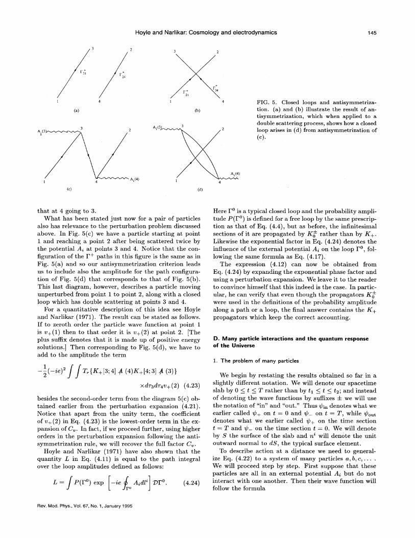
Hoyle and Narlikar: Cosmology and electrodynamics 145
A, (
(a)
I'IG. 5. Closed loops and antisymmetriza-tion. (a) and (b) illustrate the result of an-tisymmetrization, which when applied to adouble scattering process, shows how a closedloop arises in (d) from antisymmetrization of(c).
(c)
A;(4)
1 . 2———ie2
T-(If+[3;41 8 (4)I~+[4; 3] 8 (3))
xdrsdr4v+(2) (4.23)
besides the second-order term from the diagram 5(c) ob-tained earher fI'o111 the perturbatlon expa1181011 (4.21).Notice that apart from the unity term, the coefIicientof v+(2) in Eq. (4.23) is the lowest-order term in the ex-pansion of C . In fact, if we proceed further, using higherorders in the perturbation expansion following the anti-symmetrization rule, we will recover the full factor C .
Hoyle and Narlikar (1971) have also shown that thequantity L in Eq. (4.11) is equal to the path integralover the loop amplitudes defined as follows:
L = P(I' ) exp I',e A;dl' 271' . —ro
(4.24)
that at 4 going to 3.What has been stated just now for a pair of particles
also has relevance to the perturbation problem discussedabove. In Fig. 5(c) we have a particle starting at point1 and reaching a point 2 after being scattered twice bythe potential A,. at points 3 and 4. Notice that the con-figuration of the I'+ paths in this figure is the same as inFig. 5(a) and so our antisymmetrization criterion leadsus to include also the amplitude for the path configura-tion of Fig. 5(d) that corresponds to that of Fig. 5(b).This last diagram, however, describes a particle movingunperturbed from point 1 to point 2, along with a closedloop which has double scattering at points 3 and 4.
For a quantitative description of this idea see Hoyleand Narlikar (1971). The result can be stated as follows.If to zeroth order the particle wave function at point 1is v+(1) then to that order it is v+(2) at point 2. [Theplus suKx denotes that it is made up of positive energysolutions. ] Then corresponding to Fig. 5(d), we have toadd to the amplitude the term
Here I" is a typical closed loop and the probability ampli-tude P(I'o) is defined for a free loop by the same prescrip-tion as that of Eq. (4.4), but as before, the infinitesimalsections of it are propagated by Ko+ rather than by K+.I ikewise the exponential factor in Eq. (4.24) denotes theinfluence of the external potential A; on the loop I', fol-lowing the same formula as Eq. (4.17).
The expression (4.12) can now be obtained fromEq. (4.24) by expanding the exponential phase factor andusing a perturbation expansion. We leave it to the readerto convince himself that this indeed is the case. In partic-ular, he can verify that even though the propagators Ko+
were used in the definitions of the probability amplitudealong a path or a loop, the final answer contains the K+propagators which keep the correct accounting.
D. Many particle interactions and the quantum responseof the Universe
1. The problem of many particles
We begin by restating the results obtained so far in aslightly difFerent notation. We will denote our spacetimeslab by 0 & t & T rather than by t-i & t & t2., and insteadof denoting the wave functions by suKxes + we will usethe notation of "in" and "out." Thus g;„denotes what weearlier called g+ on t = 0 and itt on t = T, while g „1denotes what we earlier called Itt+ on the time sectiont = T and g on the time section t = 0. We will denoteby S the surface of the slab and n' will denote the unitoutward normal to dS, the typical surface element.
To describe action at a distance we need to general-ize Eq. (4.22) to a system of many particles a, 6, c, . . . .We will proceed step by step. First suppose that theseparticles are all in an external potential A; but do notinteract with one another. Then their wave function wIllfollow the formula
Rev. Mod. Phys. , Vol. 67, No. 1, January 1995
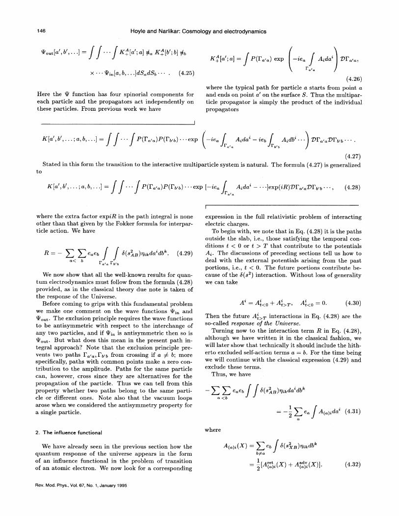
146 Hoyle and Narlikar: Cosmology and electrodynamics
4 „t[a', b', . . .] = K+"[a'; a] y. K+" [bI; b] ybK+[a';a] = P(1 ) exp —ie A;da' BI'
x . @;„[a,b, . . .]dS dSb . . (4 25)
Here the 4' function has four spinorial components foreach particle and the propagators act independently onthese particles. From previous work we have
(4.26)where the typical path for particle a starts from point aand ends on point a' on the surface S. Thus the multipar-ticle propagator is simply the product of the individualpropagators
K [a', b', . . . ; a, b, . . .] = A.,da' —iebbjb
to
(4.27)Stated in this form the transition to the interactive multiparticle system is natural. The formula (4.27) is generalized
K [a', b', . . . ; a, b, . . .] = P(I' r )P(I'b(b) exp [—ie
a'aA, da — ]exp(iB)171 171 b b (4.28)
where the extra factor expiB in the path integral is noneother than that given by the Fokker formula for interpar-ticle action. We have
B= —) ) eebb
b(s~e) q,bda*db" (4.29).
We now show that all the well-known results for quan-tum electrodynamics must follow from the formula (4.28)provided, as in the classical theory due note is taken ofthe response of the Universe.
Before coming to grips with this fundamental problemwe make one comment on the wave functions 4;„and4 „t. The exclusion principle requires the wave functionsto be antisymmetric with respect to the interchange ofany two particles, and if 0';„ is antisymmetric then so is
But what does this mean in the present path in-tegral approach? Note that the exclusion principle pre-vents two paths I', 1 b b from crossing if a g b; morespecifically, paths with common points make a zero con-tribution to the amplitude. Paths for the same particlecan, however, cross since they are alternatives for thepropagation of the particle. Thus we can tell from thisproperty whether two paths belong to the same parti-cle or di8'erent ones. Note also that the vacuum loopsarose when we considered the antisymmetry property fora single particle.
expression in the full relativistic problem of interactingelectric charges.
To begin with, we note that in Eq. (4.28) it is the pathsoutside the slab, i.e., those satisfying the temporal con-ditions t & 0 or t ) T that contribute to the potentialsA;. The discussions of preceding sections tell us how todeal with the external potentials arising from the pastportions, i.e. , t ( 0. The future portions contribute be-cause of the b'(s ) interaction. Without loss of generalitywe can take
& —&~ 0+ &~)T A«o —0. (4.3O)
e eb b(s„'~)g;b da'db"
= ——) e A( );da' (4.31)1
Then the future A~&& interactions in Eq. (4.28) are theso-called response of the Universe
Turning now' to the interaction term B in Eq. (4.28),although we have written it in the classical fashion, wewill later show that technically it should include the hith-erto excluded self-action terms a = b. For the time beingwe will continue with the classical expression (4.29) andexclude these terms.
Thus, we have
2. The influence functional where
We have already seen in the previous section how thequantum response of the universe appears in the formof an in8uence functional in the problem of transitionof an atomic electron. We now look for a corresponding
A( );(X) = ) eb b(sX~)g;bdb"bga
= —[A("),(X) + A( );(X)]. (4.32)
Rev. Mod. Phys. , Vol. 67, No. 1; January 1995
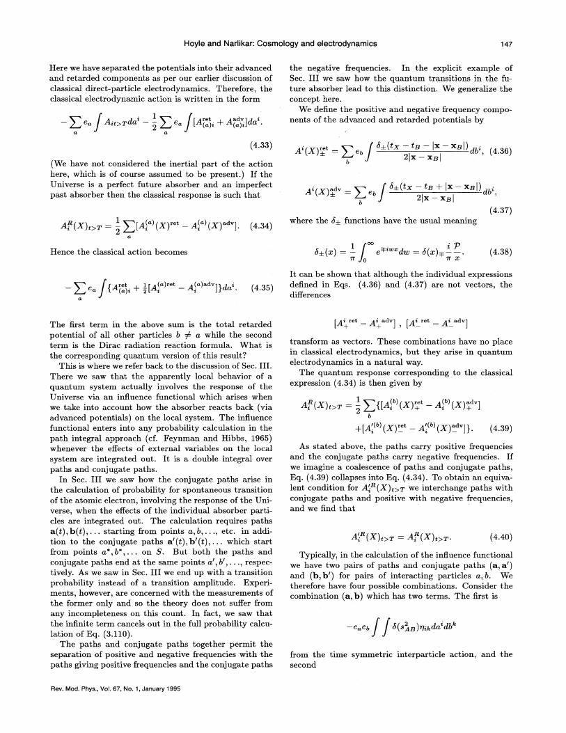
Hoyle and Narlikar: Cosmology and electrodynamics 147
Here we have separated the potentials into their advancedand retarded components as per our earlier discussion ofclassical direct-particle electrodynamics. Therefore, theclassical electrodynamic action is written in the form
the negative frequencies. In the explicit example ofSec. III we saw how the quantum transitions in the fu-ture absorber lead to this distinction. We generalize theconcept here.
We define the positive and negative &equency compo-nents of the advanced and retarded potentials by
(4.33)
(We have not considered the inertial part of the actionhere, which is of course assumed to be present. ) If theUniverse is a perfect future absorber and an imperfectpast absorber then the classical response is such that
A (X),&T = —) [A (X)"' —A (X) ]. (4.34)
f "]" " '" "'"v ]4M]b
A*(x)~ = ) ebb
4(tx —t& + Ix —x~ I)
(4.37)where the b~ functions have the usual meaning
Hence the classical action becomes (4.3S)
figI+ l]~(-)"t ~( ) ~
]iga
(4.35)
It can be shown that although the individual expressionsdefined in Eqs. (4.36) and (4.37) are not vectors, thedifferences
The first term in the above sum is the total retardedpotential of all other particles 6 g a while the secondterm is the Dirac radiation reaction formula. What isthe corresponding quantum version of this results
This is where we refer back to the discussion of Sec. III.There we saw that the apparently local behavior of aquantum system actually involves the response of theUniverse via an influence functional which arises whenwe take into account how the absorber reacts back (viaadvanced potentials) on the local system. The influencefunctional enters into any probability calculation in thepath integral approach (cf. Feynman and Hibbs, 1965)whenever the e8'ects of external variables on the localsystem are integrated out. It is a double integral overpaths and conjugate paths.
In Sec. III we saw how the conjugate paths arise inthe calculation of probability for spontaneous transitionof the atomic electron, involving the response of the Uni-verse, when the efFects of the individual absorber parti-cles are integrated out. The calculation requires pathsa(t), b(t), . . . starting from points a, b, . . ., etc. in addi-tion to the conjugate paths a'(t), b'(t), . . . which startfrom points a*,b*, . . . on S. But both the paths andconjugate paths end at the same points a', 6', . . ., respec-tively. As we saw in Sec. III we end up with a transitionprobability instead of a transition amplitude. Experi-ments, however, are concerned with the measurements ofthe former only and so the theory does not sufFer fromany incompleteness on this count. In fact, we saw thatthe infinite term cancels out in the full probability calcu-lation of Eq. (3.110).
The paths and conjugate paths together permit theseparation of positive and negative frequencies with thepaths giving positive frequencies and the conjugate paths
Ap(x)„= -') ~[AI'l(x);" —AI'~(x)'. ]b
+[A' (X)"'—A,'.'
(X) ]). (4.39)
As stated above, the paths carry positive &equenciesand the conjugate paths carry negative frequencies. Ifwe imagine a coalescence of paths and conjugate paths,Eq. (4.39) collapses into Eq. (4.34). To obtain an equiva-lent condition for A'; (X)t&T we interchange paths withconjugate paths and positive with negative frequencies,and we find that
A,'
{X)t&T = A, (X)t&z. {4.4O)
Typically, in the calculation of the influence functionalwe have two pairs of paths and conjugate paths (a, a')and (b, b') for pairs of interacting particles a, b We.therefore have four possible combinations. Consider thecombination (a, b) which has two terms. The first is
&b 0 8~~ 'l7 IcCLG l6
&om the time symmetric interparticle action, and thesecond
[Ai ret Ai adv] [Ai ret Ai adv]
transform as vectors. These combinations have no placein classical electrodynamics, but they arise in quantumelectrodynamics in a natural way.
The quantum response corresponding to the classicalexpression (4.34) is then given by
Rev. Mod. Phys. , Vol. 67, No. 1, January 1995
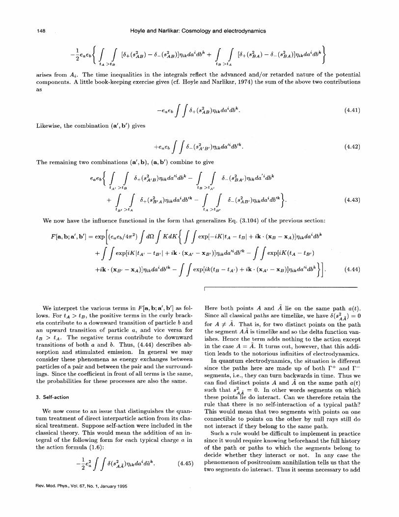
Hoyle and Narlikar: Cosmology and electrodynamics
2tw &ta
[~+(s~~) —~-("~~)]~'~«'db" + I&+(~pA) —~ ('-a~)]p ~~~ ~6")
arises from A;. The time inequalities in the integrals re8ect the advanced and/or retarded nature of the potentialcomponents. A little book-keeping exercise gives (cf. Hoyle and Narlikar, 1974) the sum of the above two contributionsas
8+ (s~~) rj, l, da'db" (4.41)
Likewise, the combination (a', b') gives
+e~eg (s~,~, )q, kdo, "db'" (4.42)
The remaining two coinbinations (a', b), (a, b') combine to give
b+ (s„',~)g;„da"db"—t~ PtA,
(s~~, )rj, l, da *db"
t~l )tQ
b+ (s~,„)g, i,da'db'"—
tA )t~l(s'„)pspd db ",o). '' (4.43)
We now have the in8uence functional in the form that generalizes Eq. (3.104) of the previous section:
pfa, b;a', b'] = exp (e eg/4m ) dB KdE( l+ik (xg —x~)]g,,da'db"
exp[i~i~~ —t~l+ ik (x& —xa )]q,y«'*db'"— exp[iK(t~ —t~ )
+'Lk (xi'~ —x~)]'g~kdn db exp[ik(t'ai —t~ ) + ik (x~ —x~)]q, j,da."db" (4.44)
3. Self-action
We now come to an issue that distinguishes the quan-tum treatment of direct interparticle action from its clas-sical treatment. Suppose self-action were included in theclassical theory. This would mean the addition of an in-tegral of the following form for each typical charge a inthe action formula (1.6):
2——e 8(s~~)g, l, do, 'do, ". (4.45)
We interpret the various terms in E[a, b; a', b'] as fol-
lows. For t~ ) t~, the positive terms in the curly brack-ets contribute to a downward transition of particle 6 andan upward transition of particle a, and vice versa for) t~. The negative terms contribute to downwardtransitions of both a and b Thus, .(4.44) describes ab-sorption and stimulated emission. In general we mayconsider these phenomena as energy exchanges betweenparticles of a pair and between the pair and the surround-ings. Since the coeKcient in front of all terms is the same,the probabilities for these processes are also the same.
Here both points A and A lie on the same path o,(t).Since all classical paths are timelike, we have b(s2 -) = 0
for A g A. That is, for two distinct points on the paththe segment AA is timelike and so the delta function van-ishes. Hence the term adds nothing to the action exceptin the case A = A. It turns out, however, that this addi-tion leads to the notorious infinities of electrodynamics.
In quantum electrodynamics, the situation is difI'erentsince the paths here are made up of both I'+ and I'segments, i.e. , they can turn backwards in time. Thus wecan find distinct points A and A on the same path a(t)such that 8 - = 0. In other words segments on whichthese points lie do interact. Can we therefore retain therule that there is no self-'interaction of a typical path?This would mean that two segments with points on oneconnectible to points on the other by null rays still donot interact if they belong to the same path.
Such a rule would be difFicult to implement in practicesince it would require knowing beforehand the full historyof the path or paths to which the segments belong todecide whether they interact or not. In any case thephenomenon of positronium annihilation tells us that thetwo segments do interact. Thus it seems necessary to add
Rev. Mod. Phys. , Vol. 67, No. 1, January 1995
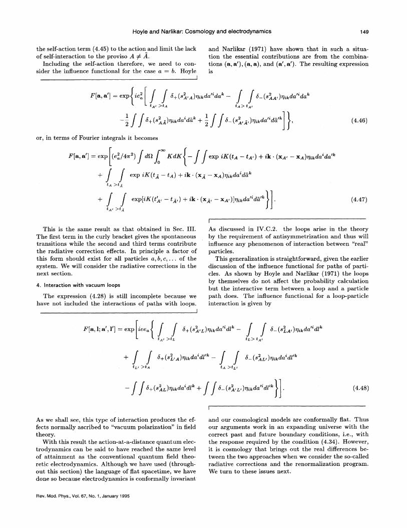
Hoyle and Narlikar: Cosmology and electrodynamics
the self-action term (4.45) to the action and limit the lackof self-interaction to the proviso A g A.
Including the self-action therefore, we need to con-sider the influence functional for the case a = b. Hoyle
I
and Narlikar (1971) have shown that in such a situa-tion the essential contributions are from the combina-tions (a, a'), (a, a), and (a', a'). The resulting expressionls
F]a, a'] = exp(te de(ss, s)st;sde"des — ftA) t~l
2b+ (s' „)g,),-da'da" +—
2(s'„, -, )g;ada" da' (4.46)
or, in terms of Fourier integrals it becomes
F]a, a'] = exp (e /4x ) fdBf KdKI —ff exp iK(ts —ts ) +ik (xs —xs)st;sd ~d e"e '
exp xK(t~ —t~) + xk. (x~ —x~)q;kda*da"
exp[i%(t&, —t&, ) +ik. (x&, —xdt, )]g;),da"da'" (4.47)
This is the same result as that obtained in Sec. III.The first term in the curly bracket gives the spontaneoustransitions while the second and third terms contributethe radiative correction effects. In principle a factor ofthis form should exist for all particles a, b, c, . . . of thesystem. We will consider the radiative corrections in thenext section.
4. Interaction with vacuum loops
The expression (4.28) is still incomplete because wehave not included the interactions of paths with loops.
I
I
As discussed in IV.C.2. the loops arise in the theoryby the requirement of antisymmetrization and thus willinfluence any phenomenon of interaction between "real"particles.
This generalization is straightforward, given the earlierdiscussion of the influence functional for paths of parti-cles. As shown by Hoyle and Narlikar (1971) the loopsby themselves do not affect the probability calculationbut the interactive term between a loop and a particlepath does. The influence functional for a loop-particleinteraction is given by
F]a, l; ', ]=aelxp ieel f
t&1 &tL,
4+(sst)stsde dl, " — f'*f 4 (sts)st;sda d!s, "tl. ) t~l
4+( , ) t dsatdxl' s—sf f 4 *( st)st;sd 'dst'se,
b+ „'~ g, I,da'dl" + (a~2, 1, )q, I, da'*dl'" (4.48)
As we shall see, this type of interaction produces the ef-fects normally ascribed to "vacuum polarization" in fieldtheory.
With this result the action-at-a-distance quantum elec-trodynamics can be said to have reached the same levelof attainment as the conventional quantum field theo-retic electrodynamics. Although we have used (through-out this section) the language of flat spacetime, we havedone so because electrodynamics is conformally invariant
and our cosmological models are conformally fat. Thusour arguments work in an expanding universe with thecorrect past and future boundary -conditions, i.e., withthe response required by the condition (4.34). However,it is cosmology that brings out the real differences be-tween the two approaches when we consider the so-calledradiative corrections and the renormalization program.We turn to these issues next.
Rev. Mod. Phys. , Vol. 67, No. 1, January 1995
150 Hoyle and Narlikar: Cosmology and electrodynamics
V. CQSMOI OGICAL RESPONSE: SOME IMPLICATIONS (5 4)
A. Radiative corrections
1. The electron self-energy correction
2——e h+ (s )rl;ada'd-a" (5.1)
describing the action of a charge a on itself. Note thatthe delta function b+ instead of 6 appears in Eq. (5.1)after we include the response of the Universe.
Any computation of a quantum electrodynamic crosssection using Eq. (5.1) leads to a divergent result if oneuses it literally as given. However, action at a distancerequires a lower cutoff of the kind
We now examine the so-called self-energy correctiondue to the radiative processes in action-at-a-distanceelectrodynamics. Recall that the classical self-energyproblem is solved in this theory by the use of advanced re-action from the rest of the Universe. The problem arisesin quantum Beld theory from the ultraviolet divergence,i.e., from the degrees of freedom of the electromagneticBeld of very high frequency. In the action-at-a-distanceversion, the self-energy problem in principle appears fromthe identification of the two legs A. , A, of the delta func-tion in the interaction
With a finite cutoff the calculation of the bare and ob-served masses of the electric charge can be performedusing the usual methods of the renormalization program.(See Hoyle and Narlikar, 1971, for details. )
The cutoff on A: at the high frequency and given by(5.3) works out to 10 sec for the atomic and cos-mological parameters described above. This cutoff mayvary from one microscopic process to another; it also islinked with the properties of the cosmic absorber. How-ever, the reasoning given above tells us that for everymicroscopic process in electrodynamics a cutoff exists.
The purely local approach to @ED demands Lorentzinvariance in every operation that may be performed.Our method, on the other hand, picks out a speciBc lo-cal reference frame, viz. the so-called cosmological restframe, to define the response of the Universe. ThusLorentz invariance is manifestly not present, althoughone can use the Lorentz transformation to describe anyprocess of @ED in a frame difFerent from the cosmologicalrest frame.
Choose the cosmological rest frame in which, by thearguments of the preceding section, all I"ourier integralsin the computations of the infiuence functional have ahigh frequency cutoff at A:, say. With c = 1, h = 1,this cutoff corresponds to a restriction in time coordinate
(5 2) ~t& —tz~ & k-.'„. (5.5)
with the cutoff vector e' having length e small comparedto the Compton wavelength of the mass m . Hoyle andNarlikar (1971) had conjectured that if a more com-
plete theory includes classical gravity then a naturalcutoff would be the Schwarzschild radius of the charge,2Gm /c . Later Padmanabhan (1985) showed that in aquantum gravity context the cutoff is the Planck length(Gh/c') '/'.
Neither of these cutoffs, however, reQect the global na-ture of the problem, i.e., the fact that any local quan-tum measurement is subject to the interference of the re-sponse of the universe. A clue to this type of cutoff wasprovided by our earlier discussion of Sec. III.E. There we
found that because of the event horizon in the future ab-sorber the response is limited to frequencies up to thosesatisfying the inequality
3e' (km b, =m~h 1+ ln
27( ( mt' )(5.6)
Notice that a similar formula comes from quantum fieldtheory but there the cutoff is a purely abstract quantityand so no numerical significance is attached to the massdifference
Zm = m.b, —m, h. (5.7)
We will shortly specify k; for the time being kremains a small quantity akin to e used in Eq. (5.2).
Using the derivation of Hoyle and Narlikar [1971: seetheir Eq. (146)] therein we find that in the cosmoIogical rest frame the observed mass m b, is related to thetheoretical mass mth of the electron by the relation
k ( u),fr/IIT, (5.3)
where' T is the time duration of the measurement. Thiswas the limit in the spontaneous transition problem.However, as we saw in Sec. IV the limit will appear in themore general inQuence functional calculated in formulas(4.44) and (4.47). This limit to high frequencies in themomentum space translates to a lower limit in the con-figuration space. Identifying the lower limit ~ in formula(5.2) with that in Eq. (5.3) we get A: 10 sec (5.8)
In the present theory k „is related to physical parame-ters and as a result it is possible to estimate it and Am,which we proceed to do now.
The upper limit on k is given by (5.3) in which we
have u,g ~ 80 sec, H 3 x 10 sec, and T a timescale large compared to the characteristic time for theprocess —in this case the free motion of the electron. Wemay take T 5/mc 10 sec. Thus we have
Rev. Mod. Phys. , Vol. 67, No. 1, January 1995
Hoyle and Narlikar: Cosmology and electrodynamics 151
Using these values, (5.6) and (5.7) give in dimensionlessform
which in turn corresponds to the current
3eln(10 ) 0.15.2' Ac
(5.9)
j'(1) = —ClqA'(1)4'= ie Tr p'K+ 13 3 K+ 31 dv3. 513
In fact, with T h/mc2, (5.9) expressed in symbols is
3n (ar.g l2~ ), II )' (5.10)
where o. is the fine-structure constant.Two comments are needed to elaborate the above con-
clusion. First, (5.10) shows clearly the cosmological inputto the correction term at which no purely local attemptto resolve the divergence problem will arrive. Second,the correction has been obtained in the cosmological restframe, and so the statement is not strictly Lorentz in-variant. This in our view is an unavoidable conclusionechoing the first comment that only a global theory canlead to the resolution of the divergence problem. In thiscontext we recall Dirac's intuitive perception when hewrote:
"With a cut off we eli-minate at once all difficulties about divergent integrals which havebeen plaguing theoretical physics for decadesThese difhculties arise only because peoplemant to have strict Iorentz invariance in animperfect theory. In doing so they are aimingfor something which may very well be impossible" [
—Dirac, 1969].
We would agree with the above sentiment with onemodification: replace the adjective "imperfect" by "in-complete" to underscore the one crucial element missedout in Beld theory, viz. the response of the Universe.
2. Charge renormalization
-(-*')(-*')ffx Tr[p'K+(2; 3) P (3)K+(3;2)]dr, dr2dr3 (5»)
with the integrations with respect to vq, w2, and v3 beingover the slab 0 & t & T. The scattering is the same asthat produced by a potential
4'(1) = ~e' ff b (s,*,)Tr(p'K (2; 3) s (3)
x K+(3; 2)]dr2drs, (5.12)
The "renormalization" of electric charge occurs in thepresent theory through the interaction of charged closedloops as intermediaries between the interaction of anytwo charges. Suppose an external potential B; scattersa particle from state ui to u2 in the presence of a loop.The loop-path inHuence functional then leads to the am-plitude
The evaluation of j'(1) is given in detail by Hoyle andNarlikar (1971) and we simply quote the result which iscutoK dependent:
2ej,(1) = ln(me) 1;(1), (5.14)
where m is the mass of the charge. The e here arisesagain from the lower limit on the separation of the twolegs of the delta function and its interpretation in terms ofthe upper limit on frequencies of the absorber responseis as given by Eqs. (5.3) and (5.4). Thus in terms ofthe cosmological parameters of the absorber we get thecharge modification Ae as
2e' (a).s lln
3~Ac (0) (5.15)
". . . this so called good theory (QED) . . . involves neglecting infinities, neglecting them inan arbitrary may. This is not sensible math-ematics. Sensible mathematics involves ne-glecting a quantity mhen it is small —not ne-glecting itjust because it is infinitely great andyou do not want it" [
—Dirac, 1978].
The proposed remedy in the present approach solvesthis outstanding difFiculty at a price that the theoreticalphysicist trained at viewing the problem in a purely lo-cal way will Bnd it difFicult to appreciate. Yet, the meritof the solution presented here should induce him to take
The result is that closed loops efFectively lower the the-oretical (or "bare" ) value of the electric charge by some0.04 fraction of its original value.
We may briefly comment on the relationship (5.4) fur-ther as follows. For A and A separated by smaller than e
the corresponding frequencies in the infIuence functionalare too high for the absorber to react and inBuence thelocal experiment. This results in slight modiBcations ofthe "bare" values of mass and charge of a typical par-ticle, for any experiment measures these values not forisolated (i.e. , bare) charges but for charges in continuousinteraction with the universe.
The renormalization program in the quantum field the-ory of charged particles has merit in that it gives an un-ambiguous way of handling infinite integrals which areonly logarithmically divergent. It has been felt that theactual values of these integrals do not contribute to ob-servable quantities and as such the success of the programis judged by how the residuals left after removing the in-finite integrals pass the observational tests. However, asDirac observed:
Rev. Mod. Phys. , Vol. 67, No. 1, January 1995
152 Hoyle and Narlikar: Cosmology and electrodynamics
into account the missing link, namely the response of theUniverse. It is this link that forces us to consider cosmo-logical boundary conditions for seemingly local problems.
B. Response calculation using the S-matrix formulation
The path integral approach of Feynman provides a nat-ural way of quantizing the %'heeler-Feynman action-at-a-distance electrodynamics, as is clear from the discussionof Secs. III and IV. Nevertheless the path integral ap-proach, especially for relativistic particles, is a relativelyunfamiliar one and one would like to see some formalcontact with the methods of quantum field theory. Thiswas provided by Davies in a series of papers (see, for ex-ample, Davies, 1970, 1971, and 1972a). We give a briefaccount of this work below.
In the first of these papers Davies discussed the ana-log of the work of Sec. III, i.e. , the formulation of thequantum response of the Universe that leads to the spon-taneous transition of the atomic electron. Starting withthe Lagrangian for the typical ath particle
L = —e ) eb b(s~~)g, ada'do,bga
and a direct particle potential due to source 6
(5.16)
AI l(X) = eg h(sx~)g;gdb",
Davies showed how to construct an S-matrix perturba-tion expansion
)-(—1)nf
x Z(X„)]de.i . dr„.
P[C(xi)C(X2)
Here P denotes a time-ordered product as usual, butthe Z(x) function cannot be the formal product of thecurrent and a potential operator since the p~ agential in
Eq. (5.17) is not a vector field in its oven rif'it. Insteadit is possible to use for 2 the basic first-order interaction
~(X) = — &l.i'(X)~(",)&l'l" (X')&,„d d '. (5.19)
Davies showed that if one uses the %'heeler-Feynmantheory and the perfect absorber condition developed inSecs. II and III above, then one can recover the usualquantum rules for direct particle fields as defined byEq. (1.9):
(o~a, (x)x„(x')~0) = —zD+(x, x') g;„, (5.2o)
(0~P [A; (X)Ak (X')]~0) = i Dp (X,X')q;g. (5.2—1)
Note that the D+ and D~ functions used here havetheir usual de6nitions in field. theory but here they have
not been used to formulate the quantum rules of A, (x)treated as operators. Instead they were deduced byDavies from the application of the response of the Uni-verse.
In subsequent papers Davies (1971, 1972a) generalizedthe formulation to give an exact expression rather than aperturbation expansion for S. In particular, in the firstof the two papers he showed that
S=Pexp —i ZX d x
=P exp —z &,"(x)D (x, x')
x ji' (W') q*"dv d7'J (5.22)
C. Experimental search for advanced potentials
Assuming the above approach to electrodynamics to bevalid, it follows that the nature of the accepted cosmologi-cal model should be consistent with the local experimentsof electrodynamics. In particular, if the cosmological re-sponse is not such as to give pure retarded solutions, thenit may be possible to detect advanced effects. There havebeen attempts to look for small advanced effects in localradiation experiments, although their interpretation it-self is shrouded in controversy.
As we saw in earlier sections, no standard big bangcosmology satisfies the absorber condition to give unam-biguous pure retarded solutions. It follows therefore thatif one of these cosmologies is right then the pure retardedsolution is untenable. Can it be that the incompletenessof future absorption would show itself through the pres-ence of small fractions of advanced effects in local exper-iments'?
Partridge (1973) attempted to detect such an effect inthe radiation of a microwave source as it alternately ra-diated into free space and a local absorber. Partridge ar-gued that advanced potentials lead to power gain ratherthan power loss in the source. Hence if a tiny fraction
gives a complete description of quantum electrodynam-ics for processes which involve only virtual photons. Notethat in the summation over all particle pairs in Eq. (5.22)the self-action is also included as was done by Hoyle andNarlikar (1971). The expression (5.22) is analogous tothat derived by Peynman (1950) by eliminating all pho-tons from the description of electrodynamics.
In the second paper Davies discussed the role of realphotons. The question is whether there are any real pho-tons at all. As Feynman put it all photons if observedover a suKciently long time scale are virtual. Thus ifthe universe is a light tight box that absorbs all photonsemitted within it then the above formalism would de-scribe all processes that apparently involve the emissionand absorption of "real" photons. The condition is basi-cally the same as that obtained by Hoyle and Narlikar,viz. that the universe should have a future absorber thatabsorbs coInpletely all photons of positive frequencies.
Rev. Mod. Phys. , Vol. 67, No. 1, January )995
Hoyle and Narlikar: Cosmology and electrodynamics 153
of radiation is via advanced potentials, the power drainfrom the source would be less than in the pure retardedcase.
Partridge set up an arrangement in which radiationwas blocked by a local absorber in one direction and wasallowed to move freely in another. The argument wasthat the local absorber will ensure pure retarded efFectswhereas the radiation into free space would travel longdistances and through an incompletely absorbing uni-verse. A switching arrangement allowed these possibil-ities alternately. Within the accuracy of the experiment(estimated at 1 part in 10 ) there was no difFerence inthe two cases. Thus Partridge claimed to have found noevidence of advanced efFects.
Subsequently, Heron and Pegg (1974) argued that Par-tridge's use of a static absorber would inevitably lead toa null result. Instead what they proposed was an exper-iment with a time asymmetric chopper absorber to alterthe boundary conditions. This would allow them to alterthe ratio of advanced to retarded components, leading toa possible detection of the former.
However, Davies (1975) has criticized both the aboveapproaches on the grounds that with proper inclusion ofthermodynamics, attempts like these are bound to givenull results. The objection raised by Davies goes in factdeeper than the specific issues relating to the proposedexperiments. Davies has argued that one cannot bypassthermodynamics as proposed by Hogarth, Hoyle, andNarlikar and that ultimately the thermodynamic asym-metry like that in the Boltzmann H theorem will have tobe included in any realistic discussion of electrodynamictime asymmetry. In other words, Davies was revertingto the explanation of time asymmetry given by Wheelerand Feynman (1945) referred to in Sec. III.
While this could be a possible line of argument itmisses the entire spirit of the action-at-a-distance theory.First, it postulates ad hoc asymmetrical initial conditionswhich are basic to the H theorem. Second, once one de-cides to work within the action-at-a-distance frameworkthe nonlocality of the problem forces one to take cog-nizance of the large scale structure of the universe, andthe cosmological considerations of Secs. III—V becomerelevant and unavoidable. The self-consistent mixtureof advanced and retarded potentials is determined by in-cluding the response of the universe. Finally, rather thanuse the statistical laws of thermodynamics as fundamen-tal laws, attempts should be made to understand themas a consequence of other more fundamental arrows oftime like electrodynamics and cosmology.
Another aspect of the Partridge-type experiment re-lates to the deeper question of a relationship of ther-modynamic and electrodynamic arrows to the expand-ing and contracting phases of a time-symmetric universe,such as the Friedmann model with A; = +1. Do thesetime arrows reverse when the universe contracts? Thisquestion, so long as one sticks to the Wheeler-Feynmanelectrodynamics, is not uniquely answered, as we saw inSec. II.C. Recently Gell-Mann and Hartle (1991) havediscussed this problem in a difFerent way. They inves-
tigate a way in which the rules of quantum mechanicsmight be adapted to impose a time symmetry on theboundary conditions. Thus when the universe enters thecontracting phase, these microscopic degrees of freedomof the universe conspire to reverse the time-asymmetricprocesses. In a reanalysis of the Partridge experimentDavies and Twamley (1993)argue that its null result goesagainst the Gell-Mann Hartle model, but suggest that amore stringent test would be to repeat the Partridge ex-periment with a laser rather than microwave antenna.This is because the universe is apparently transparentout to great distances at the 0Hz frequencies and to in-clude i'ts absorptive efFects along the future light cone ina more significant way much higher frequencies should beused.
Vl. CONCLUSION
The above remarks motivate an important extensionof the action-at-a-distance concept to all basic interac-tions of physics, so that the thermodynamics of macro-scopic systems can be understood as a consequence of thelargest scale time asymmetry, viz. the expansion of theuniverse. Thus one needs to go deeper into the controver-sial issue (see Gold, 1968, for a discussion) as to whetherin a contracting universe thermodynamics goes in the re-verse direction. There are other compelling reasons forseeking such an extension, since, so far as electrodynam-ics is concerned, action at a distance has now demon-strated the following advantages over the field theoreticdescription:
(1) The choice of retarded solutions is not ad hoc as inGeld theory but dictated by the time asymmetry of theuniverse.
(2) There is no paradox involving infinities due to self-action in the classical theory.
(3) The theory is able to account for all classical as wellas quantum electrodynamics without the extra degrees offreedom vested in free Gelds, i.e., it is more economicalin its postulates.
(4) The cosmological boundary conditions provide thecutofF at high frequencies and thereby eliminate the diver-gences that normally plague quantum electrodynamics.
(5) The concept of the response of the universe pro-vides a powerful tool for limiting viable cosmologicalmodels.
These advantages are sufhcient to motivate the gener-alization of action at a distance to other areas of physics.
There is one further hint of the possible role of the re-sponse of the universe in local phenomena, a role thattakes us beyond electrodynamics. The discussions ofSecs. III—V tell us that it is not proper to talk of a prob-ability amplitude for a local microscopic system. Thecorrect description of the physical behavior of the sys-tem follows from the probability calculation that includesthe response of the universe. Thus one is dealing with a"square of the amplitude" type of expression rather thanthe amplitude itself.
Rev. Mod. Phys. , Vot. 67, No. 1, January 1995
Hoyle and Narlikar: Cosmology and electrodynamics
This may explain the mystery that surrounds suchepistemological issues like the collapse of the urave function. What is missing from the usual discussion of theproblem is the response of the universe. The wave-function collapse represents the Bnal course of actiontaken by the system consistent with the response of theuniverse. We suggest this idea as a way of understand-ing many other conceptual issues of quantum mechan-ics. It may well be that the real nonlocal "hidden vari-ables" are contained. in the response of the universe. Fora detailed discussion of this idea see Hoyle (1982) andNarlikar (1993b).
What has been the progress towards extending theaction-at-a-distance formulation to other interactions?In the late sixties Narlikar (1968) showed how to con-struct an action-at-a-distance counterpart for a field the-ory of arbitrary spin having a quadratic Lagrangian andlinear field equations. Such a formulation will natu-rally have an absorber theory" similar to the Wheeler-Feynman theory. Earlier Narlikar (1962) had discussedan absorber theory involving neutrinos on lines similar tovirtual photons assuming that the neutrinos travel withthe speed of light and mediate in weak interactions.
Hoyle and Narlikar (1964b, 1966, and 1974) haveshown how to obtain a theory of inertia and. gravity by anatural extension to scalar conformally invariant theory.The theory reduces in the many particle approximationto general relativity with the additional demonstrationthat the sign of the gravitational constant has to be pos-itive. The theory is Machian in origin in the sense that itrelates the inertia of matter to the large scale structureof the universe.
More recently, Hoyle, Burbidge, and Narlikar (1995)have further generalized the formulation to describe thecreation of matter, including the deduction of the cosmo-logical constant. Here the creation is through the basicunit of Planck mass (hc/G) I which subsequently decaysthrough a series of high energy physics interactions tobaryonic matter —a process yet to be determined by theparticle physicists. This may very well involve a "grandunification" but through action at a distance instead ofBelds.
Perhaps the stiQ'est resistance to the concept of actionat a distance would come today not from microphysicsbut from cosmology. As we found earlier, all the popularbig bang models fail to meet the appropriate temporalboundary conditions while the steady-state model satis-Bes them. However, the latter Inodel has several difFicul-ties in explaining the observed large scale features of theuniverse. (So does the big bang idea; but it has gainedacceptance because of the belief that only it can providean explanation for the microwave background and theabundances of light nuclei, which had baReR the steady-state model. )
Recently, however, Hoyle, 8urbidge, and Narlikar(1993, 1994a, 1994b) have produced the so-called "quasi-steady-state cosmology" (QSSC) that appears to circum-vent the difFiculties faced by the steady-state model. Thismodel combines some features of the big bang model with
some of the steady-state model. It is thus able to explainobserved features like the microwave background, abun-dances of light nuclei, the redshift magnitude relation forgalaxies, radio source counts, angular size redshift rela-tion, etc. , that are normally claimed as successes of thebig bang cosmology. It also explains features which thebig bang cosmology finds hard to accommodate like theage distribution of galaxies, baryonic dark matter, rela-tionship to high energy astrophysics, and above all theexplanation of the primary creation of matter within aframework that respects the law of conservation of mat-ter and energy.
Although not claimed as "the cosmology" by its au-thors, the QSSC therefore is indicative of the kind ofcosmology that may be required to accommodate thegrowing list of extragalactic phenomena being discov-ered. For the present work, it has the merit of havingthe right kind of cosmological response. We thereforeend this article with the hope that in the growing inter-action between fundamental physics and cosmology theaction-at-a-distance approach may have a lot to oKer toboth the disciplines.
REFERENCES
Bjorken, J.D. , and S.D. Drell, 1965, Relativistic QuantumFields (McGraw Hill, New York).
Bondi, H. , and T. Gold, 1948, Mon. Not. R. Astron. Soc. 108,252.
Brans, C., and R.H. Dicke, 1961, Phys. Rev. 124, 125.Davies, P.C.W. , 1970, Proc. Camb. Phil. Soc. 68, 751.Davies, P.C.W. , 1971, 3. Phys. A 4, 836.Davies, P.C.W. , 1972a, 3. Phys. A 5, 1025.Davies, P.C.W. , 1972b, 3. Phys. A 5, 1722.Davies, P.C.W. , 1973, Mon. Not. R. Astron. Soc. 161, l.Davies, P.C.W. , 1975, 3. Phys. A 8, 272.Davies, P.C.W. , and J. Twamley, 1993, Class. Quantum Grav-
ity 10, 931.DeWitt, B.S., and R.W. Brehme, 1961, Ann. Phys. (USA) 9,
220.Dirac, P.A.M. , 1935, The Principles of Quantum Mechanics
(Clarendon, Oxford).Dirac, P.A.M. , 1938a, Proc. R. Soc. A 165, 199.Dirac, P.A.M. , 1938b, Proc. R. Soc. A 167, 148.Dirac, P.A.M. , 1969, in Eundamenta/ Interactiona at High En-
ergy, edited by T. Gudehus, G. Kaiser, and A. Perlmutter(Gordon and Breach, New York), p. 1.
Dirac, P.A.M. , 1978, in Directions in Physics (Wiley, NewYork), p. 36.
Einstein, A. , and W. deSitter, 1932, Proc. Natl. Acad. Sci.18, 213~
Feynrnan, R.P., 1949, Phys. Rev. 76, 749.Feynman, R.P., 1950, Phys. Rev. 80, 440.Feynman, R.P. , 1963, private communication.Feynman, R.P. , and A.R. Hibbs, 1965, Quantum Mechanics
and Path Integrats (McGraw Hill, New York).Fokker, A.D., 1929a, Z. Phys. 58, 386.Fokker, A.D. , 1929b, Physica 9, 33.Fokker, A.D. , 1932, Physica 12, 145.Friedrnan, A. , 1922, Z. Phys. 10, 37?.
Rev. Mod. Phys. , Yol. 6?, No. 1, January 1995
Hoyle and Narlikar: Cosmology and electrodynamics
Friedman, A. , 1924, Z. Phys. 2l. , 326.Gauss, C.F., 1867, Werke 5, 629.Gell-Mann, M. , and J.B. Hartle, 1991, Santa Barbara Report
No. UCSBTH —91—31.Gold, T., 1968, The Nature of Time (Cornell University,
Ithaca).Heron, M.L., and D.T. Pegg, 1974, J. Phys. A 7, 1965.Hogarth, J.E., 1962, Proc. R. Soc. London A 314, 529.Hoyle, F., 1948, Mon. Not. R. Astron. Soc. 108, 372.Hoyle, F., 1982, Annu. Rev. Astron. Astrophys. 20, 1.Hoyle, F., G. Burbidge, and J.V. Narlikar, 1993, Astrophys.J. 410, 437.
Hoyle, F., G. Burbidge, and J.V. Narlikar, 1994a, Mon. Not.R. Astron. Soc. 267, 1007.
Hoyle, F., G. Burbidge, and J.V. Narlikar, 1994b, Astron.Astrophys. 289, 729.
Hoyle, F., G. Burbidge, and J.V. Narlikar, 1995, Proc. R. Soc.A (in press).
Hoyle, F., and J.V. Narlikar, 1963, Proc. R. Soc. London A277 1.
Hoyle, F., and J.V. Narlikar, 1964a, Proc. R. Soc. London A282, 184.
Hoyle, F., and J.V. Narlikar, 1964b, Proc. R. Soc. London A282, 191.
Hoyle, F., and J.V. Narlikar, 1966, Proc. R. Soc. London A294) 138.
Hoyle, F., and J.V. Narlikar, 1969, Ann. Phys (NY.) 54, 207.
Hoyle, F., and J.V. Narlikar, 1971, Ann. Phys. (NY) 62, 44.Hoyle, F., and J.V. Narlikar, 1974, Action at a Die/ance in
Physics and Cosmology (Freeman, New York).Hoyle, F., and J.V. Narlikar, 1993, Proc. R. Soc. London A
442, 469.Hubble, E.P. , 1929, Proc. Nat. Acad. Sci. 15, 168.Infeld, L., and A. Schild, 1945, Phys. Rev. 68, 250.Narlikar, J.V., 1962, Proc. R. Soc.' London A 270, 553.Narlikar, J.V. , 1968, Proc. Camb. Phil. Soc. 64, 1071.Narlikar, J.V., 1974, J. Phys. A 7, 1274.Narlikar, J.V. , 1993a, Introduction to Cosmology (Cambridge
University, Cambridge, England).Narlikar, J.V., 1993b, in Philosophy of Science: Perspectives
from ¹turai and Social Sciences, edited by J.V. Narlikar, L.Banga, and C. Gupta (Indian Institute of Advanced Study,Shimla), p. 69.
Padmanabhan, T., 1985, G.B.G. Journal 17, 215.Partridge, R.B., 1973, Nature 244, 263.Roe, P.E., 1969, Mon. Not. R. Astron. Soc. 144, 219.Schwarzschild, K., 1903, Gottinger Nachrichten 128, 132.Synge, J.L., 1960, Relativity: The Genera/ Theory (North-
Holland, Amsterdam).Tetrode, H. , 1922, Z. Phys. 10, 317.Wheeler, J.A. , and R.P. Feynman, 1945, Rev. Mod. Phys. 17,
157.Wheeler, J.A. , and R.P. Feynman, 1949, Rev. Mod. Phys. 21,
425.
Rev. Mod. Phys. , Vol. 67, No. 1, January 3995