Embed Size (px)
Citation preview
.
COSMOLOGY
Lecturer: Professor Komissarov S.SRoom: 10.19 in Maths Satellite
email: [email protected]
(2012)

Contents
Contents 2
1 The Structure and Contents of Visible Universe 71.1 Structure of visible Universe . . . . . . . . . . . . . . . . . . . . . . . . . . . . . . . . . . 71.2 Expansion of visible Universe . . . . . . . . . . . . . . . . . . . . . . . . . . . . . . . . . 101.3 Contents of visible Universe . . . . . . . . . . . . . . . . . . . . . . . . . . . . . . . . . . 11
2 Gravity and Space-Time 132.1 Space and time of Newtonian physics . . . . . . . . . . . . . . . . . . . . . . . . . . . . . 13
2.1.1 Space . . . . . . . . . . . . . . . . . . . . . . . . . . . . . . . . . . . . . . . . . . 132.1.2 Time . . . . . . . . . . . . . . . . . . . . . . . . . . . . . . . . . . . . . . . . . . 152.1.3 Galilean relativity . . . . . . . . . . . . . . . . . . . . . . . . . . . . . . . . . . . . 162.1.4 The lack of speed limit . . . . . . . . . . . . . . . . . . . . . . . . . . . . . . . . . 162.1.5 Light . . . . . . . . . . . . . . . . . . . . . . . . . . . . . . . . . . . . . . . . . . 16
2.2 Special relativity . . . . . . . . . . . . . . . . . . . . . . . . . . . . . . . . . . . . . . . . 172.3 General Relativity . . . . . . . . . . . . . . . . . . . . . . . . . . . . . . . . . . . . . . . . 21
3 Friedmann’s equations 253.1 Metric of the Universe . . . . . . . . . . . . . . . . . . . . . . . . . . . . . . . . . . . . . 253.2 Derivation of Friedmann’s equations in General Relativity . . . . . . . . . . . . . . . . . . 28
4 Basic Cosmological Models 314.1 Einstein’s static Universe . . . . . . . . . . . . . . . . . . . . . . . . . . . . . . . . . . . . 314.2 Key parameters of the Universe. . . . . . . . . . . . . . . . . . . . . . . . . . . . . . . . . 32
4.2.1 Expansion and deceleration parameters . . . . . . . . . . . . . . . . . . . . . . . . 324.2.2 Critical density . . . . . . . . . . . . . . . . . . . . . . . . . . . . . . . . . . . . . 34
4.3 The Friedmann models . . . . . . . . . . . . . . . . . . . . . . . . . . . . . . . . . . . . . 364.3.1 Flat Universe . . . . . . . . . . . . . . . . . . . . . . . . . . . . . . . . . . . . . . 364.3.2 Closed Universe . . . . . . . . . . . . . . . . . . . . . . . . . . . . . . . . . . . . 374.3.3 Open Universe . . . . . . . . . . . . . . . . . . . . . . . . . . . . . . . . . . . . . 38
4.4 The Big Bang . . . . . . . . . . . . . . . . . . . . . . . . . . . . . . . . . . . . . . . . . . 394.5 Advanced topic: Cosmic microwave background radiation . . . . . . . . . . . . . . . . . . 40
4.5.1 Relic radiation . . . . . . . . . . . . . . . . . . . . . . . . . . . . . . . . . . . . . 404.5.2 Black body spectrum . . . . . . . . . . . . . . . . . . . . . . . . . . . . . . . . . . 414.5.3 History of CMB radiation . . . . . . . . . . . . . . . . . . . . . . . . . . . . . . . 424.5.4 Evolution of CMB radiation after decoupling with matter . . . . . . . . . . . . . . . 43
4.6 Some other stages of Big Bang . . . . . . . . . . . . . . . . . . . . . . . . . . . . . . . . . 444.6.1 Nucleosynthesis . . . . . . . . . . . . . . . . . . . . . . . . . . . . . . . . . . . . 444.6.2 Structure formation . . . . . . . . . . . . . . . . . . . . . . . . . . . . . . . . . . . 44
3
5 Measuring the Universe 455.1 Distances to sources with given redshift . . . . . . . . . . . . . . . . . . . . . . . . . . . . 455.2 The cosmological horizon . . . . . . . . . . . . . . . . . . . . . . . . . . . . . . . . . . . . 465.3 The angular size distance . . . . . . . . . . . . . . . . . . . . . . . . . . . . . . . . . . . . 475.4 The luminosity distance . . . . . . . . . . . . . . . . . . . . . . . . . . . . . . . . . . . . . 495.5 Supernovae and the deceleration parameter . . . . . . . . . . . . . . . . . . . . . . . . . . 51
6 Secret components of the Universe 536.1 Dark Matter . . . . . . . . . . . . . . . . . . . . . . . . . . . . . . . . . . . . . . . . . . . 536.2 Dark Energy . . . . . . . . . . . . . . . . . . . . . . . . . . . . . . . . . . . . . . . . . . . 54
7 The phase of inflation 597.1 The problems of Friedmann Cosmology . . . . . . . . . . . . . . . . . . . . . . . . . . . . 59
7.1.1 The flatness problem . . . . . . . . . . . . . . . . . . . . . . . . . . . . . . . . . . 597.1.2 The horizon problem . . . . . . . . . . . . . . . . . . . . . . . . . . . . . . . . . . 60
7.2 Inflation . . . . . . . . . . . . . . . . . . . . . . . . . . . . . . . . . . . . . . . . . . . . . 61
8 Supplemental material: Newtonian Gravity and Cosmology 638.1 Newton’s Universal Gravity . . . . . . . . . . . . . . . . . . . . . . . . . . . . . . . . . . . 63
8.1.1 The Newton’s law of gravity . . . . . . . . . . . . . . . . . . . . . . . . . . . . . . 638.1.2 Gravitational field of a spherically symmetric mass distribution . . . . . . . . . . . 65
8.2 Derivation of Friedmann’s equations from Newton’s Theory of Gravity . . . . . . . . . . . . 678.2.1 The Hubble law . . . . . . . . . . . . . . . . . . . . . . . . . . . . . . . . . . . . . 678.2.2 The Friedmann equation . . . . . . . . . . . . . . . . . . . . . . . . . . . . . . . . 688.2.3 The fluid equation . . . . . . . . . . . . . . . . . . . . . . . . . . . . . . . . . . . 698.2.4 The acceleration equation . . . . . . . . . . . . . . . . . . . . . . . . . . . . . . . 708.2.5 Newton’s law of gravity with cosmological constant . . . . . . . . . . . . . . . . . 708.2.6 The key inconsistencies of the Newtonian Cosmology . . . . . . . . . . . . . . . . 70
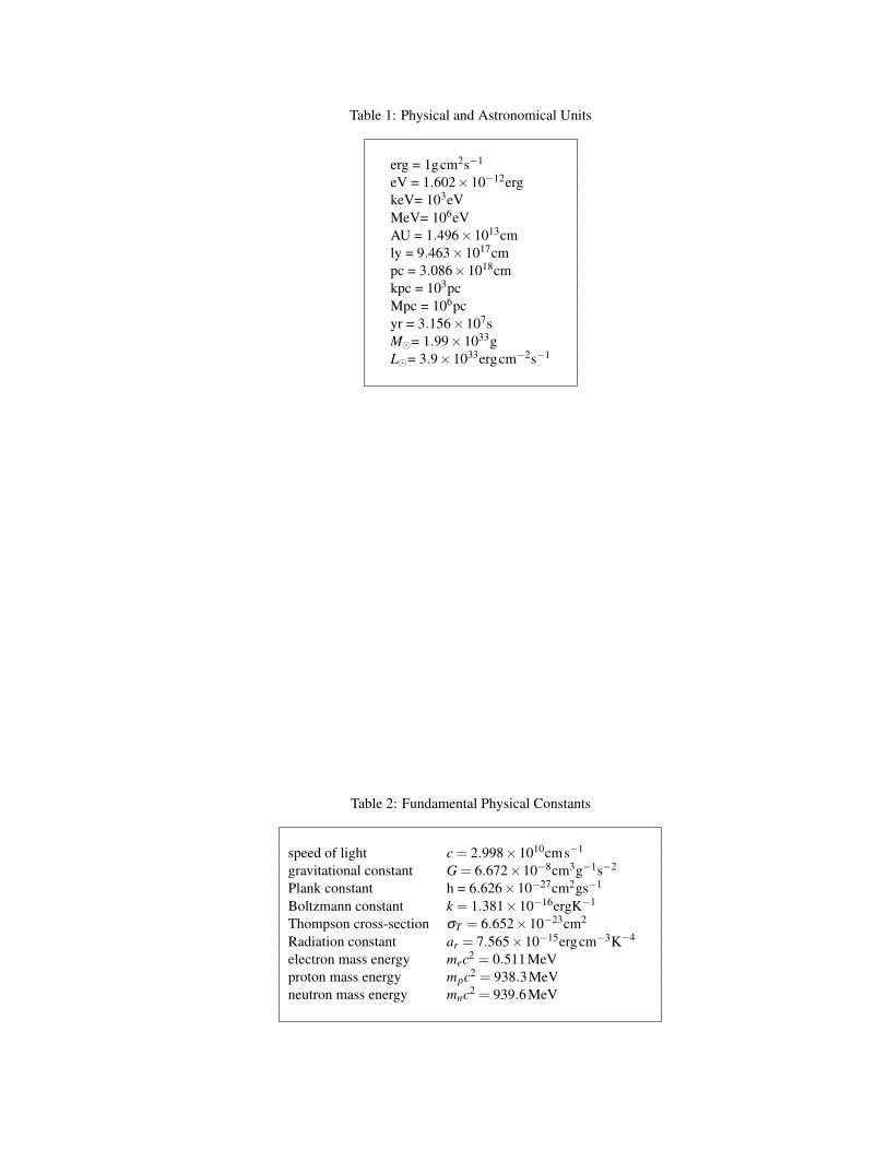
Table 1: Physical and Astronomical Units
erg = 1gcm2s−1
eV = 1.602×10⁻¹²ergkeV= 103eVMeV= 106eVAU = 1.496×10¹³cmly = 9.463×10¹⁷cmpc = 3.086×10¹⁸cmkpc = 103pcMpc = 106pcyr = 3.156×10⁷sM= 1.99×1033gL= 3.9×1033ergcm−2s−1
Table 2: Fundamental Physical Constants
speed of light c = 2.998×10¹⁰cms−1
gravitational constant G = 6.672×10⁻⁸cm3g−1s−2
Plank constant h = 6.626×10⁻²⁷cm2gs−1
Boltzmann constant k = 1.381×10⁻¹⁶ergK−1
Thompson cross-section σT = 6.652×10⁻²³cm2
Radiation constant ar = 7.565×10⁻¹⁵ergcm−3K−4
electron mass energy mec2 = 0.511MeVproton mass energy mpc2 = 938.3MeVneutron mass energy mnc2 = 939.6MeV

Chapter 1
The Structure and Contents of VisibleUniverse
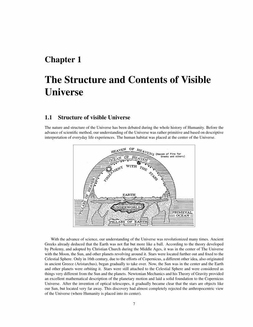
1.1 Structure of visible UniverseThe nature and structure of the Universe has been debated during the whole history of Humanity. Before theadvance of scientific method, our understanding of the Universe was rather primitive and based on descriptiveinterpretation of everyday life experiences. The human habitat was placed at the center of the Universe.
With the advance of science, our understanding of the Universe was revolutionized many times. AncientGreeks already deduced that the Earth was not flat but more like a ball. According to the theory developedby Ptolemy, and adopted by Christian Church during the Middle Ages, it was in the center of The Universewith the Moon, the Sun, and other planets revolving around it. Stars were located further out and fixed to theCelestial Sphere. Only in 16th century, due to the efforts of Copernicus, a different other idea, also originatedin ancient Greece (Aristarchus), began gradually to take over. Now, the Sun was in the center and the Earthand other planets were orbiting it. Stars were still attached to the Celestial Sphere and were considered asthings very different from the Sun and the planets. Newtonian Mechanics and his Theory of Gravity providedan excellent mathematical description of the planetary motion and laid a solid foundation to the CopernicusUniverse. After the invention of optical telescopes, it gradually became clear that the stars are objects likeour Sun, but located very far away. This discovery had almost completely rejected the anthropocentric viewof the Universe (where Humanity is placed into its center).
7
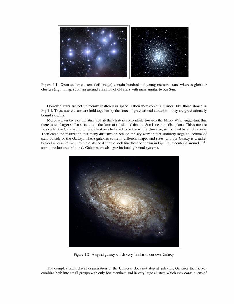
Figure 1.1: Open stellar clusters (left image) contain hundreds of young massive stars, whereas globularclusters (right image) contain around a million of old stars with mass similar to our Sun.
However, stars are not uniformly scattered in space. Often they come in clusters like those shown inFig.1.1. These star clusters are hold together by the force of gravitational attraction - they are gravitationallybound systems.
Moreover, on the sky the stars and stellar clusters concentrate towards the Milky Way, suggesting thatthere exist a larger stellar structure in the form of a disk, and that the Sun is near the disk plane. This structurewas called the Galaxy and for a while it was believed to be the whole Universe, surrounded by empty space.Then came the realization that many diffusive objects on the sky were in fact similarly large collections ofstars outside of the Galaxy. These galaxies come in different shapes and sizes, and our Galaxy is a rathertypical representative. From a distance it should look like the one shown in Fig.1.2. It contains around 1011
stars (one hundred billions). Galaxies are also gravitationally bound systems.
Figure 1.2: A spiral galaxy which very similar to our own Galaxy.
The complex hierarchical organization of the Universe does not stop at galaxies, Galaxies themselvescombine both into small groups with only few members and in very large clusters which may contain tens of
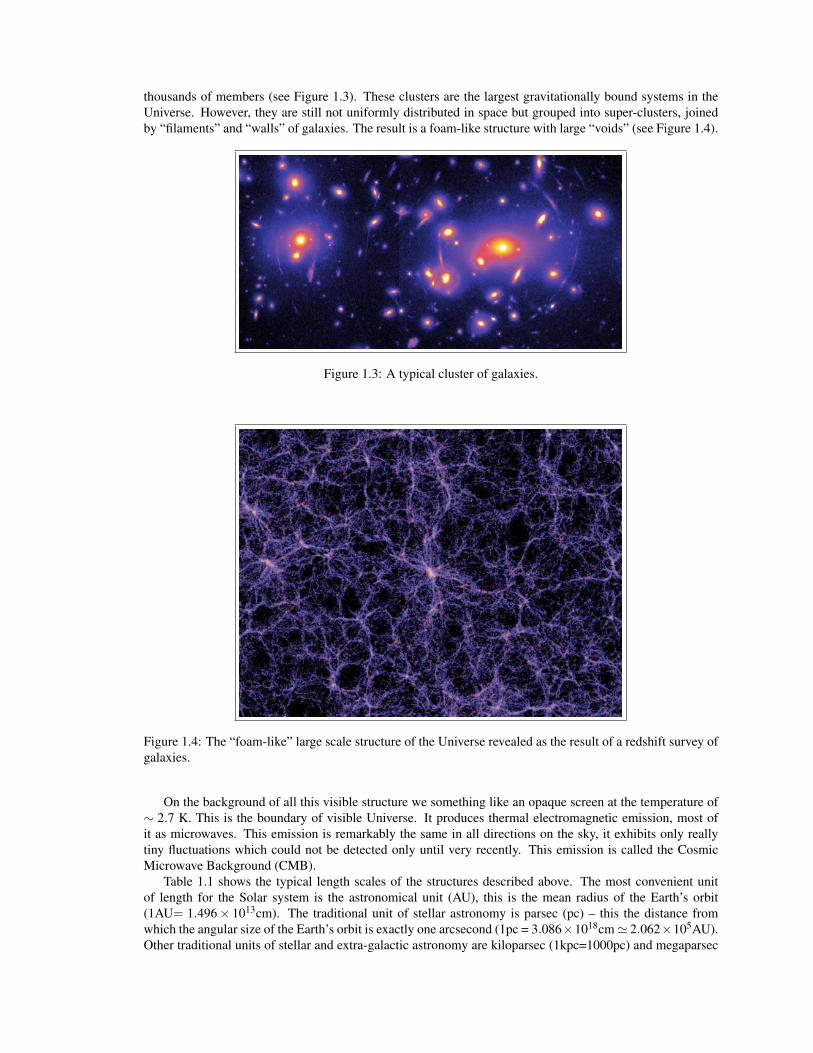
thousands of members (see Figure 1.3). These clusters are the largest gravitationally bound systems in theUniverse. However, they are still not uniformly distributed in space but grouped into super-clusters, joinedby “filaments” and “walls” of galaxies. The result is a foam-like structure with large “voids” (see Figure 1.4).
Figure 1.3: A typical cluster of galaxies.
Figure 1.4: The “foam-like” large scale structure of the Universe revealed as the result of a redshift survey ofgalaxies.
On the background of all this visible structure we something like an opaque screen at the temperature of∼ 2.7 K. This is the boundary of visible Universe. It produces thermal electromagnetic emission, most ofit as microwaves. This emission is remarkably the same in all directions on the sky, it exhibits only reallytiny fluctuations which could not be detected only until very recently. This emission is called the CosmicMicrowave Background (CMB).
Table 1.1 shows the typical length scales of the structures described above. The most convenient unitof length for the Solar system is the astronomical unit (AU), this is the mean radius of the Earth’s orbit(1AU= 1.496× 1013cm). The traditional unit of stellar astronomy is parsec (pc) – this the distance fromwhich the angular size of the Earth’s orbit is exactly one arcsecond (1pc = 3.086×1018cm' 2.062×10⁵AU).Other traditional units of stellar and extra-galactic astronomy are kiloparsec (1kpc=1000pc) and megaparsec
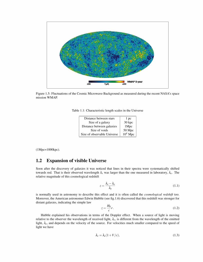
Figure 1.5: Fluctuations of the Cosmic Microwave Background as measured during the recent NASA’s spacemission WMAP.
Table 1.1: Characteristic length scales in the Universe
Distance between stars 1 pcSize of a galaxy 30 kpc
Distance between galaxies 1MpcSize of voids 50 Mpc
Size of observable Universe 104 Mpc
(1Mpc=1000kpc).
1.2 Expansion of visible UniverseSoon after the discovery of galaxies it was noticed that lines in their spectra were systematically shiftedtowards red. That is their observed wavelength λr was larger than the one measured in laboratory, λe. Therelative magnitude of this cosmological redshift
z =λr−λe
λe(1.1)
is normally used in astronomy to describe this effect and it is often called the cosmological redshift too.Moreover, the American astronomer Edwin Hubble (see fig.1.6) discovered that this redshift was stronger fordistant galaxies, indicating the simple law
z =H0
cr . (1.2)
Hubble explained his observations in terms of the Doppler effect. When a source of light is movingrelative to the observer the wavelength of received light, λr, is different from the wavelength of the emittedlight, λe, and depends on the velocity of the source. For velocities much smaller compared to the speed oflight we have
λr = λe(1+V/c), (1.3)
andz =
Vc
(1.4)
where c is the speed of light and V is the radial component of velocity (positive when the distance increasesand negative otherwise). This is known as the Doppler effect. It can be used to measure the source motionwhen most other methods fail and it is particularly useful in astronomy, dealing with very distant sources.(In fact, when the spectrum of the source radiation is a featureless continuum this effect is not easy to useeither. Fortunately, in many cases the spectrum contains very fine features, emission and absorption lines,reflecting the quantum nature of atoms, and this allows to make very accurate speed measurements.) Onecan see that if the source is moving away than λr > λe, and thus the optical lines are shifted towards longerwavelengths, or towards the red end of the spectrum. So Hubble concluded that distant galaxies move awayfrom us. Combining Eq.1.2 with Eq.1.4 we find that
V = H0r . (1.5)
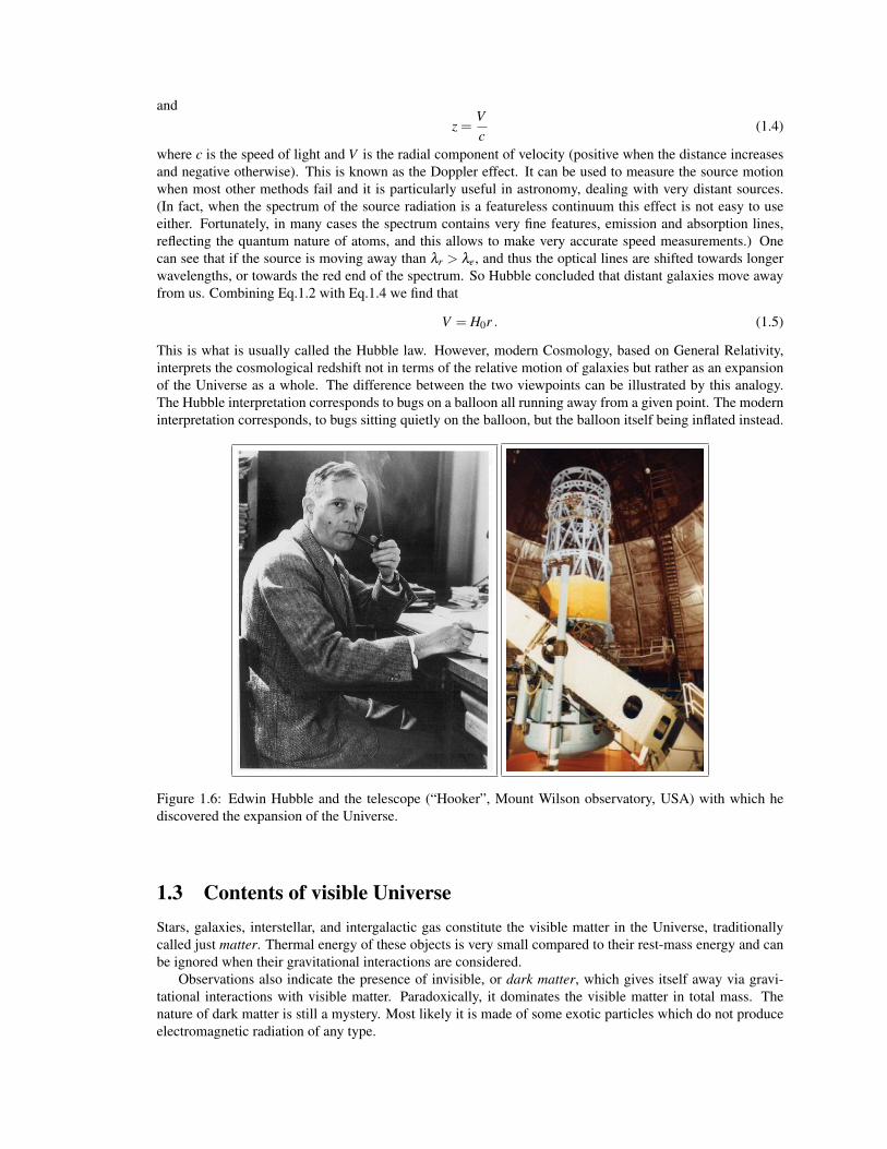
This is what is usually called the Hubble law. However, modern Cosmology, based on General Relativity,interprets the cosmological redshift not in terms of the relative motion of galaxies but rather as an expansionof the Universe as a whole. The difference between the two viewpoints can be illustrated by this analogy.The Hubble interpretation corresponds to bugs on a balloon all running away from a given point. The moderninterpretation corresponds, to bugs sitting quietly on the balloon, but the balloon itself being inflated instead.
Figure 1.6: Edwin Hubble and the telescope (“Hooker”, Mount Wilson observatory, USA) with which hediscovered the expansion of the Universe.
1.3 Contents of visible UniverseStars, galaxies, interstellar, and intergalactic gas constitute the visible matter in the Universe, traditionallycalled just matter. Thermal energy of these objects is very small compared to their rest-mass energy and canbe ignored when their gravitational interactions are considered.
Observations also indicate the presence of invisible, or dark matter, which gives itself away via gravi-tational interactions with visible matter. Paradoxically, it dominates the visible matter in total mass. Thenature of dark matter is still a mystery. Most likely it is made of some exotic particles which do not produceelectromagnetic radiation of any type.
Then there is electromagnetic radiation (photons), Cosmic Rays and other relativistic particles which aresimilar in some important respects to photons. To be more specific, their rest mass-energy is only a smallfraction of their total mass-energy, and therefore can ignored in gravitational interactions. We will explain themeaning of rest mass-energy later on. In Cosmology, all these relativistic components are generally referredto as radiation.
Finally, there seems to exist another exotic component which dominates even the dark matter in terms ofits effect on the evolution of the Universe at present time – the so called dark energy. In contrast to all othercomponents it’s gravity is repulsive. We will discuss both the dark matter and dark energy later in the course.
Chapter 2
Gravity and Space-Time
The evolution of the Universe is described by the Einstein’s General Relativity. This is a rather complicatedtheory and requires a high level of mathematical preparation. Therefore, only a very brief description of theTheory of Relativity and its application to Cosmology will be given here, with most results presented withoutderivation.
2.1 Space and time of Newtonian physics
2.1.1 SpaceThe abstract notion of physical space reflects the properties of physical objects to have sizes and physicalevents to be located at different places relative to each other. In Newtonian physics, the physical space wasconsidered as a fundamental component of the world around us, which exists by itself independently of otherphysical bodies and normal matter of any kind. It was assumed that 1) one could “interact” with this spaceand unambiguously determine the motion of objects in this space, in addition to the easily observed motionof physical bodies relative to each other, 2) that one may introduce points of this space, and determine atwhich point any particular event took place. The actual ways of doing this remained mysterious though. Itwas often thought that the space is filled with a primordial substance, called “ether” or “plenum”, which canbe detected one way or another, and that “atoms” of ether correspond to points of physical space and thatmotion relative to these atoms is the motion in physical space. This idea of physical space was often called“the absolute space” and the motion in this space “the absolute motion”.
There also was a consensus that the best mathematical model for the absolute space was the 3-dimensionalEuclidean space. By definition, in such space one can construct cuboids, rectangular parallelepipeds, suchthat the lengths of their edges, a,b, and c, and the diagonal l satisfy the following equation
l2 = a2 +b2 + c2, (2.1)
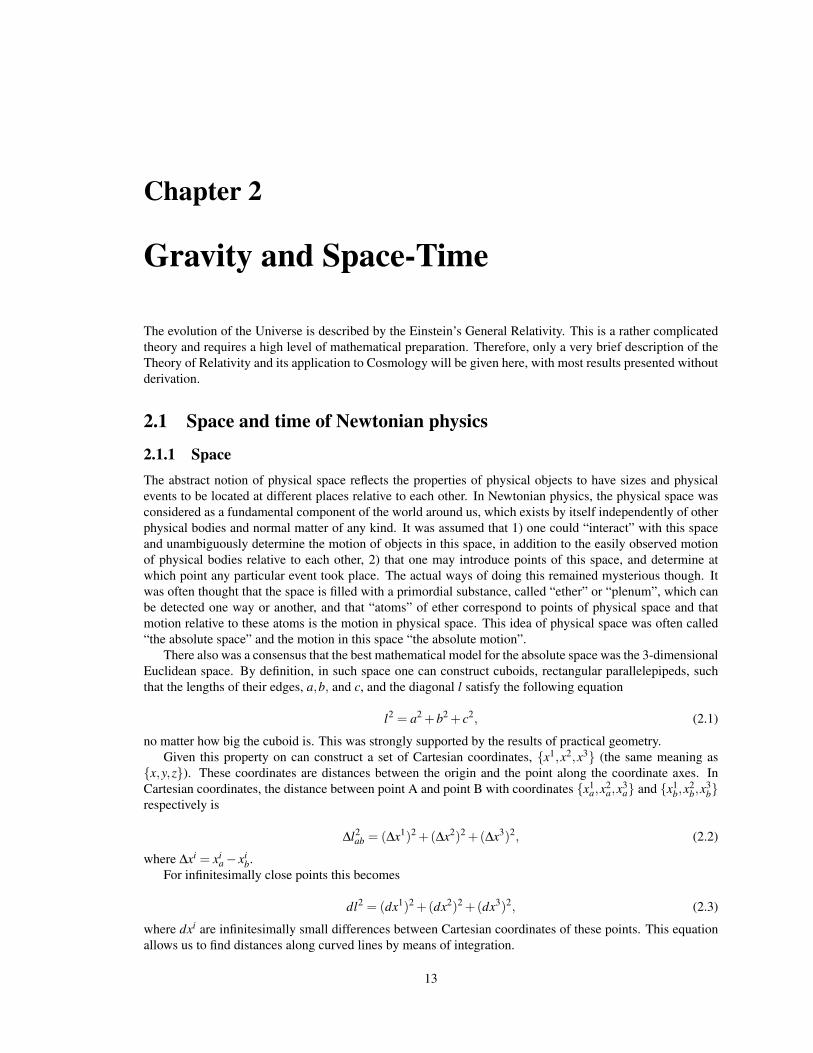
no matter how big the cuboid is. This was strongly supported by the results of practical geometry.Given this property on can construct a set of Cartesian coordinates, x1,x2,x3 (the same meaning as
x,y,z). These coordinates are distances between the origin and the point along the coordinate axes. InCartesian coordinates, the distance between point A and point B with coordinates x1
a,x2a,x
3a and x1
b,x2b,x
3b
respectively is
∆l2ab = (∆x1)2 +(∆x2)2 +(∆x3)2, (2.2)
where ∆xi = xia− xi
b.For infinitesimally close points this becomes
dl2 = (dx1)2 +(dx2)2 +(dx3)2, (2.3)
where dxi are infinitesimally small differences between Cartesian coordinates of these points. This equationallows us to find distances along curved lines by means of integration.
13
xx
x
x
x
x
Figure 2.1: Cartesian coordinates
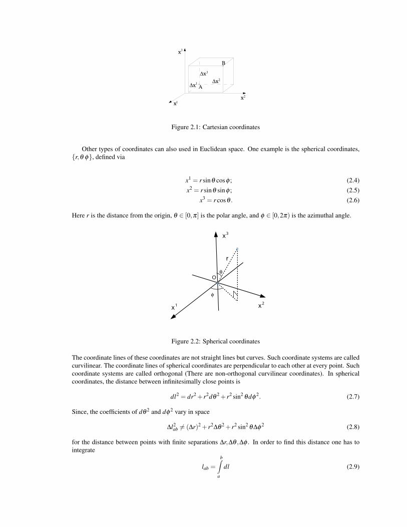
Other types of coordinates can also used in Euclidean space. One example is the spherical coordinates,r,θ φ, defined via
x1 = r sinθ cosφ ; (2.4)x2 = r sinθ sinφ ; (2.5)
x3 = r cosθ . (2.6)
Here r is the distance from the origin, θ ∈ [0,π] is the polar angle, and φ ∈ [0,2π) is the azimuthal angle.
O
x
x
1
3
r
x2
Figure 2.2: Spherical coordinates
The coordinate lines of these coordinates are not straight lines but curves. Such coordinate systems are calledcurvilinear. The coordinate lines of spherical coordinates are perpendicular to each other at every point. Suchcoordinate systems are called orthogonal (There are non-orthogonal curvilinear coordinates). In sphericalcoordinates, the distance between infinitesimally close points is
dl2 = dr2 + r2dθ2 + r2 sin2
θdφ2. (2.7)
Since, the coefficients of dθ 2 and dφ 2 vary in space
∆l2ab 6= (∆r)2 + r2∆θ
2 + r2 sin2θ∆φ
2 (2.8)
for the distance between points with finite separations ∆r,∆θ ,∆φ . In order to find this distance one has tointegrate
lab =
b∫a
dl (2.9)
along the line connecting these points. For example the circumference of a circle of radius r0 is
∆l =∫
dl = 2π∫
0
r0dθ = 2πr0 . (2.10)
(Notice that we selected such coordinates that the circle is centered on the origin, r = r0, and it is in ameridional plane, φ =const. As the result, along the circle dl = r0dθ .)
In the generic case of curvilinear coordinates, the distance between infinitesimally close points is givenby the positive-definite quadratic form
dl2 =3
∑i=1
3
∑j=1
gi jdxidx j, (2.11)
where the coefficients gi j = g ji are normally functions of the coordinates xi. Such quadratic forms are calledmetric forms. gi j are in fact the components of so-called metric tensor in the coordinate basis of utilizedcoordinates. It is easy to see that in a Cartesian basis
gi j = δi j =
1 if i = j0 if i 6= j (2.12)
Not all positive definite metric forms correspond to Euclidean space. If there does not exist a coordinatetransformation which reduces a given metric form to that of Eq.2.3 then the space with such metric form isnot Euclidean. This mathematical result is utilized in General Relativity.
2.1.2 TimeThe notion of time reflects our everyday-life observation that all events can be placed in a particular orderreflecting their causal connection. In this order, event A appears before event B if A caused B or could causeB. This causal order seems to be completely independent on the individual analyzing these events. This notionalso reflects the obvious fact that one event can last longer then another one. In Newtonian physics, time wasconsidered as a kind of fundamental ever going process, presumably periodic, so that one can compare therate of this process to rates of all other processes. Although the nature of this process remained mysteriousit was assumed that all other periodic processes, like the Earth rotation, reflected it. Given the fundamentalnature of time it would be natural to assume that this process occurs in ether.
This understanding of time has lead naturally to the absolute meaning of simultaneity. That is one couldunambiguously decide whether two events were simultaneous or not. Similarly, physical events could beplaced in only one particular order, so that if event A precedes event B according to the observation of someobserver, this has to be the same for all other observers, unless a mistake is made. Similarly, any event couldbe described by only one duration, when the same unit of time is used to quantify it. These are the reasonsfor the time of Newtonian physics to be called the “absolute time”. There is only one time for everyone.
Both in theoretical and practical terms, a unique temporal order of events could only be established if thereexisted signals propagating with infinite speed. In this case, when an event occurs in a remote place everyonecan become aware of it instantaneously by means of such “super-signals”. Then all events immediately divideinto three groups with respect to this event: (i) The events simultaneous with it – they occur at the same instantas the arrival of the super-signal generated by the event; (ii) The events preceding it – they occur before thearrival of this super-signal and could not be caused by it. But they could have caused the original event; (iii)The events following it – they occur after the arrival of this super-signal and can be caused by it. But theycannot cause the original event.
If, however, there are no such super-signals, things become highly complicated as one needs to know notonly the distances to the events but also the motion of the observer and how exactly the signals propagatedthrough the space separating the observer and these events. Newtonian physics assumes that such infinitespeed signals do exist and they play fundamental role in interaction between physical bodies. This is howin the Newtonian theory of gravity, the gravity force depends only on the current location of the interactingmasses.
2.1.3 Galilean relativity
Galileo, who is regarded to be the first true natural scientist, made a simple observation which turned out tohave far reaching consequences for modern physics. He noticed that it was difficult to tell whether a ship wasanchored or coasting at sea by means of mechanical experiments carried out on board of this ship.
It is easy to determine where a body is moving through air – in the case of motion, it experiences the airresistance, the drag and lift forces. But here we are dealing only with a motion relative to air. What about themotion relative to the absolute space and the interaction with ether? If such an interaction occurred then onecould measure the “absolute motion”. Galileo’s observation tells us that this must be at least a rather weekinteraction. No other mechanical experiment, made after Galileo, has been able to detect such an interaction.Newtonian mechanics adopts the Galilean relativity via introducing the so-called inertial frames, which coastwith constant speed through the absolute space. All laws of Newtonian mechanics have exactly the same formin all these frames. For example, the motion of a physical body which does not interact with other bodiesremains unchanged. It moves with constant speed along straight line. This means that one cannot determinethe motion through absolute space by mechanical means. Only the relative motion between physical bodiescan be determined this way.
2.1.4 The lack of speed limit
Is there any speed limit a physical body can have in Newtonian mechanics? The answer to this question isNo. To see this consider a particle of mass m under the action of constant force f . According to the secondlaw of Newton its speed then grows linearly,
v = v0 +fm
t,
without a limit.This conclusion also agrees with the Galilean principle of relativity. Indeed, suppose the is a maximum
allowed speed, say vmax. According to this principle it must be the same for all inertial frames. Now considera body moving with such a speed to the right of the frame S. This frame can also move with speed vmax tothe right relative to the frame S. Then according to the Galilean velocity addition this body moves relative tothe frame S with speed 2vmax. This contradicts to our assumption that there exist a speed limit, and hence thisassumption has to be discarded.
2.1.5 Light
The nature of light was a big mystery in Newtonian physics and a subject of heated debates between scientists.One point of view was that light is made by waves propagating in ether, by analogy with sound which ismade by waves in air. The speed of light waves was a subject of great interest to scientists. The most naturalexpectation for waves in ether is to have infinite speed. Indeed, waves with infinite speed fit nicely the conceptof absolute time, and if such waves exist then there is no more natural medium for such waves as the etherof absolute space. However, the light turned out to have finite speed. Dutch astronomer Roemer noticed thatthe motion of Jupiter’s moons had systematic variation, which could be easily explained only if one assumedthat light had finite, though very large, speed. Since then, many other measurements have been made whichall agree on the value for the speed of light
c' 3×1010cm/s .
The development of mathematical theory of electromagnetism resulted in the notions of electric and mag-netic fields, which exist around electrically charged bodies. These fields do not manifest themselves in anyother ways but via forces acting on other electrically charged bodies. Attempts do describe the properties ofthese fields mathematically resulted in Maxwell’s equations, which agreed with experiments most perfectly.
What is the nature of electric and magnetic field? They could just reflect some internal properties ofmatter, like air, surrounding the electrically charged bodies. Indeed, it was found that the electric and mag-netic fields depended on the chemical and physical state of surrounding matter. However, the experiments
clearly indicated that the electromagnetic fields could also happily exist in vacuum (empty space). This factprompted suggestions that in electromagnetism we are dealing with ether.
Analysis of Maxwell equations shows that electric and magnetic fields change via waves propagating withfinite speed. In vacuum the speed of these waves is the same in all direction and equal to the known speedof light! When this had been discovered, Maxwell immediately interpreted light as electromagnetic waves orether waves. Since according to the Galilean transformation the result of any speed measurement depends onthe selection of inertial frame, the fact that Maxwell equations yielded a single speed could only mean thatthey are valid only in one particular frame, the rest frame of ether and absolute space. On the other hand, thefact that the astronomical observations and laboratory experiments did not find any variation of the speed oflight as well seemed to indicate that Earth was almost at rest in the absolute space.
SunEarth
Vorb
VorbSun
Earth Vorb
2Vorb
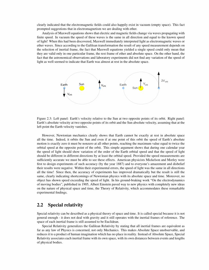
Figure 2.3: Left panel: Earth’s velocity relative to the Sun at two opposite points of its orbit. Right panel:Earth’s absolute velocity at two opposite points of its orbit and the Sun absolute velocity, assuming that at theleft point the Earth velocity vanishes.
However, Newtonian mechanics clearly shows that Earth cannot be exactly at rest in absolute spaceall the time. Indeed, it orbits the Sun and even if at one point of this orbit the speed of Earth’s absolutemotion is exactly zero it must be nonzero at all other points, reaching the maximum value equal to twice theorbital speed at the opposite point of the orbit. This simple argument shows that during one calendar yearthe speed of light should show variation of the order of the Earth orbital speed and that the speed of lightshould be different in different directions by at least the orbital speed. Provided the speed measurements aresufficiently accurate we must be able to see these effects. American physicists Mickelson and Morley werefirst to design experiments of such accuracy (by the year 1887) and to everyone’s amazement and disbelieftheir results were negative. Within their experimental errors, the speed of light was the same in all directionsall the time! Since then, the accuracy of experiments has improved dramatically but the result is still thesame, clearly indicating shortcomings of Newtonian physics with its absolute space and time. Moreover, noobject has shown speed exceeding the speed of light. In his ground-braking work “On the electrodynamicsof moving bodies”, published in 1905, Albert Einstein paved way to new physics with completely new ideason the nature of physical space and time, the Theory of Relativity, which accommodates these remarkableexperimental findings.
2.2 Special relativity
Special relativity can be described as a physical theory of space and time. It is called special because it is notgeneral enough - it does not deal with gravity and it still operates with the inertial frames of reference. Thespace of each inertial frame is still assumed to be Euclidean.
Special Relativity generalizes the Galilean Relativity by stating that all inertial frames are equivalent asfar as any law of Physics is concerned, not only Mechanics. This makes Absolute Space unobservable, andreduces it to a product of human imagination which has no place in reality. Instead of Absolute Space, SpecialRelativity associates each inertial frame with its own space, with its own distances between events and lengthsof physical bodies.
As an example of application of this principle suppose that in a particular frame it is established that thereis maximum possible speed that a physical object can have. Then in any other frame there must exist exactlythe same maximum possible speed. In fact, Special Relativity yields such speed. It equals to the speed oflight in vacuum, c. Our every day experience speaks against this idea. For example the speed of a car movingalong the road as measured relative to a stationary police patrol car is different from that measured relativeto a moving patrol car. However, in our every day life we are dealing with speeds which are much less thanc. This is a singular limit where the true nature of motion is not revealed. On the other hand, the physicalexperiments designed to deal with very high speeds show that the speed of light is indeed invariant. Moreover,there has been no observations of speeds exceeding the speed of light so far.
The requirement for the speed of light to be the same in all inertial frames immediately leads to a numberof spectacular results.
• Relativity of simultaneity: Events simultaneous in one frame may not be simultaneous in another. Thisimplies that time interval between events depends on the inertial frame used for time measurements(recall that all frames are equipped with clocks manufactured to the same standards). That there is nounique temporal order of physical events and that each inertial frame has its own time.
• Time dilation: Consider a standard clock moving relative to some inertial frame with speed v. Supposethat the time displayed by the clock’s screen increases from τ to τ +∆τ (τ is called the proper time ofthis clock). The corresponding time interval recorded by the clock grid of this frame, ∆t, is larger bythe factor
γ = (1− v2/c2)−1/2,
which is called the Lorentz factor. That is,
∆t = γ∆τ. (2.13)
• Length contraction: Consider a solid rod of length l0 as measured using standard measuring toolsmoving together with the rod, this is called the proper length of the rod. When identical standardmeasuring tools are used by observers at rest in the inertial frame relative to which the rod is movingwith speed v the result depend on the rod orientation. When the rod is positioned perpendicular to thedirection of motion its length is the same,
l = l0. (2.14)
When the rod is aligned with the direction of motion its length is smaller,
l =l0γ. (2.15)
For intermediate angles l0/γ < l < l0.
• Invariance of the spacetime interval. Consider any two events and measure their separation in spaceand time, ∆l and ∆t. The effects of time dilation and length contraction show that these quantities aredifferent in different inertial frames. However, their combination
∆s2 =−c2∆t2 +∆l2. (2.16)
turns out to be the same! Surely, this remarkable result must be significant! In fact, it tells us thatspace and time can be united into a single 4-dimensional metric space with ∆s being the generalizeddistance between points (events) in this space. This space is called Minkowskian spacetime, after themathematician who introduced it.
Since ∆l2 = ∆x2 +∆y2 +∆z2 we can write
∆s2 =−c2∆t2 +∆x2 +∆y2 +∆z2. (2.17)
For infinitesimally closed points this becomes
ds2 =−c2dt2 +dx2 +dy2 +dz2. (2.18)
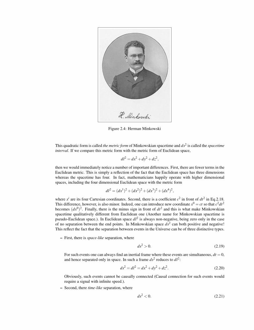
Figure 2.4: Herman Minkowski
This quadratic form is called the metric form of Minkowskian spacetime and ds2 is called the spacetimeinterval. If we compare this metric form with the metric form of Euclidean space,
dl2 = dx2 +dy2 +dz2,
then we would immediately notice a number of important differences. First, there are fewer terms in theEuclidean metric. This is simply a reflection of the fact that the Euclidean space has three dimensionswhereas the spacetime has four. In fact, mathematicians happily operate with higher dimensionalspaces, including the four dimensional Euclidean space with the metric form
dl2 = (dx1)2 +(dx2)2 +(dx3)2 +(dx4)2,
where xi are its four Cartesian coordinates. Second, there is a coefficient c2 in front of dt2 in Eq.2.18.This difference, however, is also minor. Indeed, one can introduce new coordinate x0 = ct so that c2dt2
becomes (dx0)2. Finally, there is the minus sign in front of dt2 and this is what make Minkowskianspacetime qualitatively different from Euclidean one (Another name for Minkowskian spacetime ispseudo-Euclidean space.). In Euclidean space dl2 is always non-negative, being zero only in the caseof no separation between the end points. In Minkowskian space ds2 can both positive and negative!This reflect the fact that the separation between events in the Universe can be of three distinctive types.
– First, there is space-like separation, where
ds2 > 0. (2.19)
For such events one can always find an inertial frame where these events are simultaneous, dt = 0,and hence separated only in space. In such a frame ds2 reduces to dl2:
ds2 = dl2 = dx2 +dy2 +dz2. (2.20)
Obviously, such events cannot be causally connected (Causal connection for such events wouldrequire a signal with infinite speed.).
– Second, there time-like separation, where
ds2 < 0. (2.21)
For such events one can always find an inertial frame where these events occur at the same place,dl = 0, and hence they are separated only in time. This time is the proper time of the standardclock of this frame, dτ . Thus, we have
ds2 =−c2dτ2 or dτ =
√−ds2/c. (2.22)
Obviously, such events can be causally connected.
– Finally, for some events one can haveds2 = 0 (2.23)
even if these events are different. This type of separation is called null. From Eq.2.16 one can seethat in this case
c2dt2 = dl2 or dl/dt = c. (2.24)
Thus, these two events can be events in the life of a photon, a particle moving with speed c.
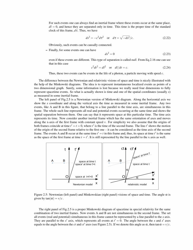
The difference between the Newtonian and relativistic visions of space and time is nicely illustrated withthe help of the Minkowski diagrams. The idea is to represent instantaneous localized events as points of atwo dimensional graph. Surely, some information is lost because we really need four dimensions to fullyrepresent spacetime events. So what is actually shown is time and one of the spatial coordinates (usually x)as measured in some inertial frame.
The left panel of Fig.2.5 is a Newtonian version of Minkowski diagram. Along the horizontal axis weshow the x coordinate and along the vertical axis the time as measured in some inertial frame. Any twoevents, like A and B in this figure, that belong to a line parallel to the time axis, are simultaneous in thisframe. The whole such line represents all real and potential events occurring at the same time and shows thespatial separation between them. One can say that it represents space at this particular time. The time axisrepresents its time. Now consider another inertial frame which has the same orientation of axes and movesalong the x-axis of the first frame with constant speed v. For simplicity we also assume that the origins ofboth frames coincide at time t ′ = t = 0, where t ′ is the time of the second frame. The line t ′ shows the motionof the origin of the second frame relative to the first one – it can be considered as the time axis of the secondframe. The events A and B occur at the same time t ′ = t in this frame and, thus, its space at time t ′ is the sameas the space of the first frame at time t = t ′. It is still represented by the line parallel to the x axis as well.
x
space at time t
t t'
O space at t=t'=0
A B
Newtonian model
space' at time t'=t
x'
x
space at time t
ct ct'
O
A Bspace' at time t'
x'
relativistic model
Figure 2.5: Newtonian (left panel) and Minkowskian (right panel) visions of space and time. The angle α isgiven by tan(α) = v/c .
The right panel of Fig.2.5 is a proper Minkowski diagram of spacetime in special relativity for the samecombination of two inertial frames. Now events A and B are not simultaneous in the second frame. The setall events (real and potential) simultaneous in this frame cannot be represented by a line parallel to the x axis.They are parallel to the x′ axis, which represents all events at t ′ = 0. The angle between the x and x′ axesequals to the angle between the ct and ct ′ axes (see Figure 2.5). If we denote this angle as α , then tanα = v/c.

Thus, the space of the second frame, is different from the space of the first frame. The spacetime is the same,but for each inertial frame it splits into space and time specific to this frame.
The revolutionized notions of space and time in Special Relativity have dramatic implications for physicsin general and particle dynamics in particular. One of the most important results is the equivalence of massand energy,
E = mc2, (2.25)
where E is the total energy of the particle and m is its inertial mass. One one hand, this famous equation tellsus that there is energy, E0, associated with the rest mass of the particle, m0, that is the inertial mass of thisparticle in the frame where it is at rest. In principle, this energy can be released and converted into other kindsof energy, for example in nuclear reactions. On the other hand, it tells us that the inertial mass, m, of movingparticle is higher than its rest mass due to the contribution from its kinetic energy. In fact, one can show that
m2 = m20 + p2/c2, (2.26)
where p is the particle momentum, p = mv, or
m = m0γ. (2.27)
This has an important implication for the inertial mass-energy density of hot gas (fluid), as the particles ofhot gas move around and hence have non-vanishing kinetic energy. Consider a frame there the macroscopicspeed of gas is zero, the so-called comoving frame. In Newtonian physics, the inertial mass density of gas inthis frame is
ρ = ρ0 = m0n,
where m0 is the rest mass of a single gas particle and n is the number density of gas particles (the number ofparticles per unit volume). In relativity, we also need to take into account the contribution due to the thermalmotion of these particles,
et =1
Γ−1P, (2.28)
where P is the gas thermal pressure and 1 < Γ < 2 is the so-called ratio of specific heats. This leads to theresult
ρ = ρ0 +(et/c2) = ρ0 +1
Γ−1(P/c2). (2.29)
The quantity given by Eq.2.29 is called the proper or comoving mass density1. For a non-relativistic gas,where the speed of thermal motion is low compared to the speed of light, vt c and the correspondingLorentz factor thermal motion γt ' 1, one has et ρ0c2, and ρ = ρ0. For an ultra-relativistically hot gas, thatis gas with the Lorentz factor of thermal motion, γt 1, the second term on the right hand side of Eq.2.26and hence the second term on the right hand side in Eq.2.29 dominate. Moreover, in this regime Γ = 4/3.Thus, one may ignore the contribution due to the rest mass and assume that
ρ = 3P/c2. (2.30)
Photons, or the particles of light, move exactly with the speed of light. Then Eqs.2.25 and 2.27 imply thatthe photon’s rest mass density m0 = 0 (otherwise its energy would be infinite). Thus, Eq.2.30, is exact forradiation, which can be considered as gas of photons.
2.3 General RelativityMass m that appears in the second law of Newtonian mechanics (Eq.8.2) is the inertial mass. The same massappears in the right hand side of the Newton’s law of gravity, Eq.8.1, where it determines the strength ofgravitational force. There is no mathematical reason for this. In fact, by analogy with electromagnetism, thelaw of gravity could involve not the inertial mass but a different quantity, that could be called gravitational
1In frames where the macroscopic speed of gas is not zero the inertial mass density is different because of the length contractioneffect and the contribution to mass due to the kinetic energy of the macroscopic motion.
charge or gravitational mass, mg. Some particles could have it, some not. Two particles with the same inertialmass could have different gravitational mass. However, in Nature
mg = m. (2.31)
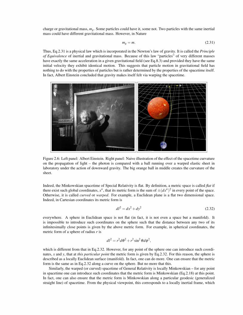
Thus, Eq.2.31 is a physical law which is incorporated in the Newton’s law of gravity. It is called the Principleof Equivalence of inertial and gravitational mass. Because of this law “particles” of very different masseshave exactly the same acceleration in a given gravitational field (see Eq.8.3) and provided they have the sameinitial velocity they exhibit identical motion. This suggests that particle motion in gravitational field hasnothing to do with the properties of particles but is rather determined by the properties of the spacetime itself.In fact, Albert Einstein concluded that gravity makes itself felt via warping the spacetime.
Figure 2.6: Left panel: Albert Einstein. Right panel: Naive illustration of the effect of the spacetime curvatureon the propagation of light – the photon is compared with a ball running over a warped elastic sheet inlaboratory under the action of downward gravity. The big orange ball in middle creates the curvature of thesheet.
Indeed, the Minkowskian spacetime of Special Relativity is flat. By definition, a metric space is called flat ifthere exist such global coordinates, xν , that its metric form is the sum of ±(dxν)2 in every point of the space.Otherwise, it is called curved or warped. For example, a Euclidean plane is a flat two dimensional space.Indeed, in Cartesian coordinates its metric form is
dl2 = dx2 +dy2 (2.32)
everywhere. A sphere in Euclidean space is not flat (in fact, it is not even a space but a manifold). Itis impossible to introduce such coordinates on the sphere such that the distance between any two of itsinfinitesimally close points is given by the above metric form. For example, in spherical coordinates, themetric form of a sphere of radius r is
dl2 = r2dθ2 + r2 sin2
θdφ2,
which is different from that in Eq.2.32. However, for any point of the sphere one can introduce such coordi-nates, x and y, that at this particular point the metric form is given by Eq.2.32. For this reason, the sphere isdescribed as a locally Euclidean surface (manifold). In fact, one can do more. One can ensure that the metricform is the same as in Eq.2.32 along a curve on the sphere. But no more that this.
Similarly, the warped (or curved) spacetime of General Relativity is locally Minkowskian – for any pointin spacetime one can introduce such coordinates that the metric form is Minkowskian (Eq.2.18) at this point.In fact, one can also ensure that the metric form is Minkowskian along a particular geodesic (generalizedstraight line) of spacetime. From the physical viewpoint, this corresponds to a locally inertial frame, which
you can imagine as a small free flying laboratory with its small Cartesian grid (confined within the labora-tory’s walls) and standard clocks. Within the walls of this laboratory the spacetime curvature has a very littleeffect and all physical phenomena are not effected by gravity. However, it is generally impossible to extendthis grid well outside of the laboratory without destroying its nice properties.
In most problems the metric form is not known before hand. So often it is written in the most generalform
ds2 =3
∑ν=0
3
∑µ=0
gνµ dxν dxµ . (2.33)
Here xν are some coordinates of spacetime (traditionally the indexes vary not from 1 to 4 but from 0 to 3),and the coefficients gνµ are functions of these coordinates. In fact, these coefficients are the components ofthe so-called metric tensor
However, this general form hides the difference between spacetime, with its time-like and space-likedirections, and other kinds of four dimensional metric manifolds. More transparent is the so-called 3+ 1representation
ds2 =−αc2dt2 +3
∑1
βidxidt +3
∑i=1
3
∑j=1
γi jdxidx j. (2.34)
Here t is considered as the global time coordinate. The hyper-surface t = t0 is considered as the global spaceat time t0. In general it is not Euclidean but warped (see the right panel of Fig.2.6). Its metric form is
dl2 =3
∑i=1
3
∑j=1
γi jdxidx j, (2.35)
with xi considered as coordinates of space (i=1,2,3). The coefficient α > 0 is called the lapse function. Inorder to understand its meaning, consider a standard clock attached to the spatial grid and consider two eventsin the life of this clock separated by the proper time dτ (the time measured by this clock). For these eventsds2 =−c2dτ2 (see Eq.2.22). On the other hand dxi = 0 and hence ds2 =−αc2dt2. Thus, we have
−c2dτ2 =−αc2dt2 or α =
(dτ
dt
)2
. (2.36)
Thus, the lapse function gives the rate of standard clocks attached to the spatial grid compared to the rate ofglobal time.
At any point of the global space one can have many different local inertial frames (or fiducial inertialobservers), each with their own local Euclidean Space. One of these frames can be considered as being atrest in the global space. Its local Euclidean space is essentially a part of the global space, meaning that eventswith dt = 0 appear simultaneous in this local inertial frame.2 Vector β , called the shift vector, gives thevelocity dxi/dt of such inertial frame relative to the global spacial grid. In general, it is impossible to haveβ = 0 everywhere.
The key equation of General Relativity is the celebrated Einstein’s equation
Rνµ −12
Rgνµ =8πGc4 Tνµ , (2.37)
which Einstein discovered in 1915. Here Rνµ is the Ricci tensor, R is the scalar curvature – they describeproperties of spacetime. In Minkowskian spacetime Rνµ = 0 and R = 0 everywhere. T νµ is called the stress-energy-momentum tensor. It describes the distribution of energy, momentum, and stresses associated withmatter, radiation, and all sorts of force fields.
The simple appearance of Einstein equation is deceptive. In fact, this is one of the most difficult equationsof Mathematical Physics, which can be solved analytically only in very limited cases of highly symmetricproblems. Only during the last decade mathematicians figured out how to solve this equation numerically. Sohere I only briefly discuss its nature.
2In mathematics, the Euclidean space of this local inertial frame is called “tangent” to the hyper-surface t = t0.
Since ν ,µ = 0 . . .3 we have sixteen equations in Eq.2.37. The Ricci tensor and the curvature scalar arefunctions of gνµ , its first and second order derivatives with respect to all four coordinates. Thus, we aredealing not with one equation but with a system of sixteen simultaneous second order partial differentialequations. The unknown functions of coordinates in these equations are gνµ and Tνµ – the Einstein equationnot only describes how matter warps spacetime but also how matter evolves in this warped spacetime.
If correct, the Einstein equation should also describe the Universe, which is filled with gravitationallyinteracting matter. In 1915 the Universe and the Milky Way (our Galaxy) were considered as the samething, and the Milky Way appeared to be very much static. Einstein analyses models of static Universe andconcluded that such Universe cannot be infinite. Instead, it must be finite but without boundaries - the spacemust be wrapped onto itself like a sphere in Euclidean geometry. Later however, he run into difficulty ashis equation 2.37 did not allow such a static solution. So he modified this equation by adding the so calledCosmological term:
Rνµ −12
Rgνµ =8πGc4 Tνµ −
Λc2 gνµ , (2.38)
where Λ is called the Cosmological constant. (In Newtonian Physics this is equivalent to introduction of arepulsive force to balance gravity.) After the Hubble’s discovery Einstein abandoned his work on the Cosmo-logical term, and called it his “biggest blunder”. However, the modern data indicate that the Cosmologicalterm is in fact needed to explain the observations.
Chapter 3
Friedmann’s equations
3.1 Metric of the UniverseThe simplest from the mathematical view point model of the Universe is where it is uniform, that is where itsgeometry is the same at every point. From the observational prospective it is not obvious that our Universe isuniform. Indeed, the very existence of the boundary of visible Universe (the CMB “screen”) seem to indicatethat it is not uniform. However, as we shell see later this observations are easily explained in the relativisticmodels of the Universe where it is assumed uniform. These models predict the observed Universe to appearisotropic (or almost isotropic) and this prediction agrees with the observations very well indeed.
What is the spacetime metric of such a Universe? As we have seen, metric of any spacetime can bewritten as
ds2 =−αc2dt2 +3
∑i=1
βidxidt +dl2, (3.1)
where dl is the line element of space (see Sec.2.3). The uniformity of universe means that one can introducesuch spacetime coordinates, t and xi, that neither α nor β depend on the spatial coordinates, but only on time.Such a coordinate system is obviously preferable. In fact there are many such coordinate systems. Amongthem are those where α = 1. Indeed, if α 6= 1 we just redefine the time coordinate so that dt ′ =
√αdt. Thus,
one can prescribe the metric as
ds2 =−c2dt ′2 +3
∑1
β′i dxidt ′+dl2. (3.2)
There are still many different coordinate systems which allow such a metric form. The isotropy of universetells us that among them there are systems where the metric form is isotropic, that is for dxi = dxi
0 anddxi =−dxi
0 we should have the same dl2 and ds2. This requires βi = 0. The result is
ds2 =−c2dt2 +dl2. (3.3)
Let us analyze this. Consider a standard clock with fixed spatial coordinates xi. If τ is the proper time of sucha clock then the spacetime interval between any two events in its life is ds2 =−c2dτ2 (see Eq.2.22). On theother hand Eq.3.16 gives ds2 = −c2dt2 for the same two events. Thus, dt = dτ , that the cosmological timet in Eq.3.16 “ticks” at the same rate as the time of standard clocks at rest relative to the spatial grid. Sincethe shift vector βi is zero the spatial grid is at rest in space. In particular, if the universe is expanding then sodoes the grid, and at exactly the same rate. Just imagine inflating a spherical balloon with a coordinate gridprinted on it and you will get the meaning of this. Our interpretation of the Hubble’s discovery will be thatthe distant galaxies are at rest in space, and hence have fixed spatial coordinates, but the distance betweenthem is increasing.
Finally, we need to figure out the metric form of the space (the hyper-surface of the spacetime determinedby the equation t =const). When Einstein was constructing his first model of the Universe he reasoned alongthe following lines. First, because of matter the spacetime and the space have to be curved. Uniformity ofthe Universe means that the curvature of space must be the same at every point. In order to guess what such
25
spaces could be, consider surfaces of 3-dimensional Euclidean space. The only two types of surfaces withuniform curvature are planes and spheres. Planes have to be excluded as they have zero curvature (they areflat). So the only relevant case is a sphere. This suggests that the geometry of the Universe must be the sameas that of a three-dimensional hyper-sphere of four-dimensional Euclidean space!
What exactly is this hyper-sphere? If xi where i = 1 . . .4 are the four Cartesian coordinates of the four-dimensional Euclidean space, centered on center of the hyper-sphere of radius R, then its equation is
(x1)2 +(x2)2 +(x3)2 +(x4)2 = R2.
Thus, the hyper-sphere is the set of all point located at the distance R from the origin. What is the metricform of such a hyper-surface? We can find it following the same steps we do in order to find the metric formof a normal sphere in three-dimensional Euclidean space.
'
O
A
x4
3D Euclidean space
4D Euclidean space
A'
'
O
A
x3
2D Euclidean space
3D Euclidean space
''
'A ''x1
x2
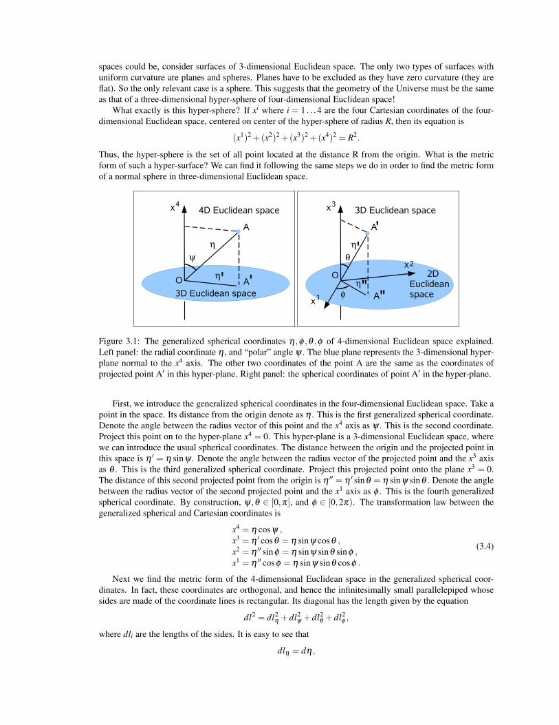
Figure 3.1: The generalized spherical coordinates η ,φ ,θ ,φ of 4-dimensional Euclidean space explained.Left panel: the radial coordinate η , and “polar” angle ψ . The blue plane represents the 3-dimensional hyper-plane normal to the x4 axis. The other two coordinates of the point A are the same as the coordinates ofprojected point A′ in this hyper-plane. Right panel: the spherical coordinates of point A′ in the hyper-plane.
First, we introduce the generalized spherical coordinates in the four-dimensional Euclidean space. Take apoint in the space. Its distance from the origin denote as η . This is the first generalized spherical coordinate.Denote the angle between the radius vector of this point and the x4 axis as ψ . This is the second coordinate.Project this point on to the hyper-plane x4 = 0. This hyper-plane is a 3-dimensional Euclidean space, wherewe can introduce the usual spherical coordinates. The distance between the origin and the projected point inthis space is η ′ = η sinψ . Denote the angle between the radius vector of the projected point and the x3 axisas θ . This is the third generalized spherical coordinate. Project this projected point onto the plane x3 = 0.The distance of this second projected point from the origin is η ′′ = η ′ sinθ = η sinψ sinθ . Denote the anglebetween the radius vector of the second projected point and the x1 axis as φ . This is the fourth generalizedspherical coordinate. By construction, ψ,θ ∈ [0,π], and φ ∈ [0,2π). The transformation law between thegeneralized spherical and Cartesian coordinates is
x4 = η cosψ ,x3 = η ′ cosθ = η sinψ cosθ ,x2 = η ′′ sinφ = η sinψ sinθ sinφ ,x1 = η ′′ cosφ = η sinψ sinθ cosφ .
(3.4)
Next we find the metric form of the 4-dimensional Euclidean space in the generalized spherical coor-dinates. In fact, these coordinates are orthogonal, and hence the infinitesimally small parallelepiped whosesides are made of the coordinate lines is rectangular. Its diagonal has the length given by the equation
dl2 = dl2η +dl2
ψ +dl2θ +dl2
φ ,
where dli are the lengths of the sides. It is easy to see that
dlη = dη ,
dlψ = ηdψ,
dlθ = η′dθ = η sinψdθ ,
dlφ = η′′dφ = η sinψ sinθdφ .
Thus, the metric form is
dl2 = dη2 +η
2dψ2 +η
2 sin2ψ(dθ
2 + sin2θdφ
2). (3.5)
Now we can find the metric form of the hyper-sphere of radius R. Since on the hyper-surface η = R anddη = 0, we have
dl2 = R2 (dψ2 + sin2
ψ(dθ2 + sin2
θdφ2)). (3.6)
Clearly, Rψ is the distance from the north pole of the hyper-sphere along the ψ coordinate line. Denote thisas r ( r varies from 0 to πR.). Then the metric form (3.6) reads
dl2 = dr2 +R2 sin2( r
R
)(dθ
2 + sin2θdφ
2) . (3.7)
This looks familiar. In fact, for r R, we have sin(r/R)→ r/R and the metric form (3.7) becomes
dl2 = dr2 + r2(dθ2 + sin2
θdφ2) , (3.8)
which is the metric form of 3-dimensional Euclidean space in spherical coordinates. Thus, our r,θ and φ areanalogues of the spherical coordinates It is illuminating to compare (3.7) with the metric form of a normalsphere in the “polar” coordinates, which we derived earlier in class,
dl2 = dρ2 +R2 sin2
(ρ
R
)dφ
2 . (3.9)
For ρ R this reduces to the metric form of 2-dimensional Euclidean space in polar coordinates. Thesimilarity is striking, but expected.
The fact that we considered a hyper-sphere of a 4-dimensional Euclidean space does not necessarilymean that our physical space is embedded into some higher dimensional physical space. We simply usedthis approach to derive the metric of a 3-dimensional space (or rather a manifold) with constant curvature.No additional physical spatial dimensions are really needed to be introduced here. (Though they may beintroduced, and they are introduced in modern physics, but for other reasons.).
Are there any other types of uniformly curved 3-dimensional manifolds? Yes. First, the trivial case of3-dimensional Euclidean space, which has zero curvature everywhere. Its metric form is given by Eq.3.8 andcan also be written as
dl2 = R2 (dψ2 +ψ
2(dθ2 + sin2
θdφ2)), (3.10)
where ψ = r/R varies from 0 to +∞. Finally, there is the so-called hyperbolic space with the metric
dl2 = R2 (dψ2 + sinh2
ψ(dθ2 + sin2
θdφ2)), (3.11)
where Ψ also varies from 0 to +∞. This also corresponds to a hyper-surface but now in the Minkowskianspacetime (also known as pseudo-Euclidean space). Its geometric properties are similar to those of a saddle-like surface in Euclidean space (see Figure 3.2).
In fact, all these three metric forms, Eqs.3.6, 3.10, and 3.11, can be written in a very similar form. Indeed,Eq.3.6 can be written as
dl2 = R2(
dχ2
1−χ2 +χ2(dθ
2 + sin2θdφ
2)
), (3.12)
where χ = sinψ ∈ [0,1], Eq.3.10 as
dl2 = R2 (dχ2 +χ
2(dθ2 + sin2
θdφ2)), (3.13)
where χ = ψ ∈ [0,+∞), and Eq.3.11 as
dl2 = R2(
dχ2
1+χ2 +χ2(dθ
2 + sin2θdφ
2)
), (3.14)
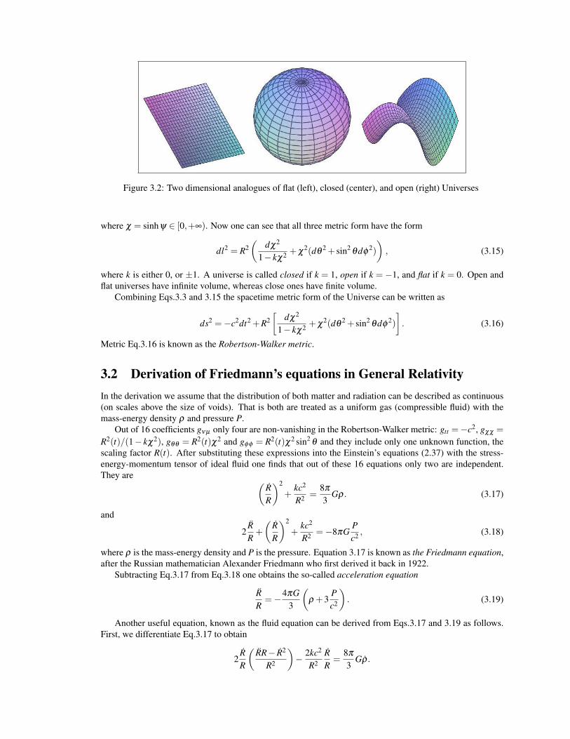
Figure 3.2: Two dimensional analogues of flat (left), closed (center), and open (right) Universes
where χ = sinhψ ∈ [0,+∞). Now one can see that all three metric form have the form
dl2 = R2(
dχ2
1− kχ2 +χ2(dθ
2 + sin2θdφ
2)
), (3.15)
where k is either 0, or ±1. A universe is called closed if k = 1, open if k = −1, and flat if k = 0. Open andflat universes have infinite volume, whereas close ones have finite volume.
Combining Eqs.3.3 and 3.15 the spacetime metric form of the Universe can be written as
ds2 =−c2dt2 +R2[
dχ2
1− kχ2 +χ2(dθ
2 + sin2θdφ
2)
]. (3.16)
Metric Eq.3.16 is known as the Robertson-Walker metric.
3.2 Derivation of Friedmann’s equations in General RelativityIn the derivation we assume that the distribution of both matter and radiation can be described as continuous(on scales above the size of voids). That is both are treated as a uniform gas (compressible fluid) with themass-energy density ρ and pressure P.
Out of 16 coefficients gνµ only four are non-vanishing in the Robertson-Walker metric: gtt =−c2, gχχ =
R2(t)/(1− kχ2), gθθ = R2(t)χ2 and gφφ = R2(t)χ2 sin2θ and they include only one unknown function, the
scaling factor R(t). After substituting these expressions into the Einstein’s equations (2.37) with the stress-energy-momentum tensor of ideal fluid one finds that out of these 16 equations only two are independent.They are (
RR
)2
+kc2
R2 =8π
3Gρ. (3.17)
and
2RR+
(RR
)2
+kc2
R2 =−8πGPc2 , (3.18)
where ρ is the mass-energy density and P is the pressure. Equation 3.17 is known as the Friedmann equation,after the Russian mathematician Alexander Friedmann who first derived it back in 1922.
Subtracting Eq.3.17 from Eq.3.18 one obtains the so-called acceleration equation
RR=−4πG
3
(ρ +3
Pc2
). (3.19)
Another useful equation, known as the fluid equation can be derived from Eqs.3.17 and 3.19 as follows.First, we differentiate Eq.3.17 to obtain
2RR
(RR− R2
R2
)− 2kc2
R2RR=
8π
3Gρ.

Figure 3.3: Alexander Friedmann
Then we substitute in the result the expressions for R from the acceleration equation and kc2/R2 from theFriedmann equation. This gives us the fluid equation
ρ =−3(
RR
)(ρ +
Pc2
). (3.20)
When the Einstein equation with the cosmological term (Eq.2.38) is used instead of the original Eq.2.37,the Friedmann and the acceleration equations become(
RR
)2
+kc2
R2 =8π
3Gρ +
Λ3, (3.21)
RR=−4πG
3
(ρ +3
Pc2
)+
Λ3. (3.22)
respectively, whereas the fluid remains unchanged.

Chapter 4
Basic Cosmological Models
4.1 Einstein’s static UniverseBack in 1917 Albert Einstein investigated whether his General Relativity can explain the observed stationaryUniverse, the contemporary astronomical data suggested that the Universe and the Milky Way were the samething. For a stationary Universe the scaling factor R must be constant and hence all its time derivatives mustvanish. However, the acceleration equation (Eq.3.19) shows that
R < 0,
as ρ,P > 0. This was the reason that had led Einstein to introduce his “cosmological term”. With this term,the Friedmann equations read (
RR
)2
+kc2
R2 =8π
3Gρ +
Λ3, (4.1)
RR=−4πG
3
(ρ +3
Pc2
)+
Λ3, (4.2)
ρ =−3(
RR
)(ρ +
Pc2
). (4.3)
Since the Milky is made of nonrelativistic matter (e.g. stars, planets, interstellar gas) P/c2 ρ and can beignored. Then Eq.4.3 becomes
ρ =−3(
RR
)ρ or
dρ
ρ=−3
dRR
.
This separable equation is easily integrated:
4π
3ρR3 = M = const. (4.4)
This result simply says that the mass of a sphere expanding with the Universe is constant. Given this we canrewrite Eqs.4.1 and 4.2 as (
RR
)2
+kc2
R2 =2GM
R3 +Λ3, (4.5)
RR=−GM
R3 +Λ3. (4.6)
Let us see if these equations allow the stationary solution
R(t) = R0.
When we substitute this into Eq.4.6 we findGMR3
0=
Λ3. (4.7)
31
Thus, the stationary solution is only possible for Λ > 0 ! Similarly, from Eq.4.5 we find that
kc2
R20=
2GMR3
0G+
Λ3
and using Eq.4.7 obtainkc2
R20= Λ. (4.8)
Thus, the stationary solution requires k = 1, which means that the Universe must be closed (see Sec.3.2)!However, this solution is unstable, as was first shown by Friedmann in 1922. To see this will use the
technique of linear stability analysis. First, consider a small perturbation around this stationary solution
R(t) = R0(1+ ε(t)) where ε 1.
Then Eq.4.6 becomes the differential equation governing the evolution of ε(t).
d2
dt2 (R0(1+ ε)) =−GMR2
0(1+ ε)−2 +
Λ3
R0(1+ ε).
Next expand (1+ ε)−2 in Taylor series keeping only the first two terms
(1+ ε)−2 = 1−2ε.
This gives us
R0ε =−GMR2
0+
Λ3
R0 +2GM
R20
ε +Λ3
R0ε.
The first two terms in the right hand side of this equation give zero (see Eq.4.7) and so we end up with theevolution equation for ε
ε = a2ε, (4.9)
wherea2 =
2GMR3
0+
Λ3> 0.
The general solution of Eq.4.9 isε =C1e+at +C2e−at ,
where C1 and C2 are constants and without any loss of generality we may assume a> 0. From this solution wecan see that at large time the perturbation grows exponentially, which shows the instability of the Einstein’sstationary solution.
4.2 Key parameters of the Universe.
4.2.1 Expansion and deceleration parametersFor non-stationary Universe, it’s key kinematic parameters are the expansion (or contraction) and deceleration(or acceleration) rates Using the Taylor expansion of R(t) for |t− t0| t0, where t0 is the current time, onehas
R(t)' R(t0)+ R0(t− t0)+12
R0(t− t0)2 = R0
[1+H0(t− t0)−
q0
2H2
0 (t− t0)2], (4.10)
where
H0 =R0
R0(4.11)
and
q0 =−R0
R0H20. (4.12)
Obviously, H0 > 0 corresponds to expanding Universe and H0 < 0 to contracting one. q0 > 0 corresponds todecelerating expansion of the Universe and q0 < 0 to its accelerating expansion. q0 is called the decelerationparameter. For Einstein’s static Universe H0 = 0 and q0 = 0.
q0 is a dimensionless parameter. The physical dimension of H0 is 1/T , the same as the dimension of theHubble constant. This is indeed the Hubble constant. In order to show this, consider two points in spaceparticipating in the expansion of the Universe. At one point we have a source of light and at the other anobserver (us). Let us use spherical coordinates centered on the observer, so that the comoving coordinate ofthe observer is χ = 0 and the comoving coordinate of the source is χe. Let us analyze the propagation of aphoton emitted by the source at time te and received at time t0. As the photon propagates radially towardsthe observer, along its trajectory in space, and hence along its worldline in spacetime we have θ =const andφ =const. Moreover, along the worldlines of photons
ds2 = 0
(see Sec.2.2). Then from the Robertson-Walker metric of the Universe, Eq.3.16, we have
−c2dt2 +R2(t)dχ2
1− kχ2 = 0.
Thus,
cdt =− R(t)dχ√1− kχ2
.
andt0∫
te
cdtR(t)
=
χe∫0
dχ√1− kχ2
. (4.13)
Now consider another photon, which is emitted a bit later, at time te +dte. It will be received a bit later too,at time t0 +dtr. Repeating the above calculations we then find
t0+dtr∫te+dte
cdtR(t)
=
χe∫0
dχ√1− kχ2
. (4.14)
From the last two equation we see that
t0+dtr∫te+dte
cdtR(t)−
t0∫te
cdtR(t)
= 0 . (4.15)
From the definition of definite integral, for any function f (t)
t0+dtr∫te+dte
f (t)dt =− f (te)dte +
t0+dtr∫te
f (t)dt =+ f (t0)dtr− f (te)dte +
t0∫te
f (t)dt.
Thus, from Eq.4.15 we havecdtrR0− cdte
R(te)= 0 or
dtrdte
=R0
R(te). (4.16)
Now imagine that instead of two separate pulses of light we are dealing with two successive crests of a lightwave with period at the source Te = dte. At the receiver its period will be Tr = dtr. Then Eq.4.16 becomes
Tr
Te=
R0
R(te).
Since the wavelength and period of a light wave are related via T = λ/c this leads to
λr
λe=
R0
R(te). (4.17)
Because t0 > te, for the expanding Universe we have R0/R(te)> 1 and thus at the receiver the wavelength islonger, explaining the effect of cosmological redshift. Using the redshift parameter z this result reads
R0
R(te)= 1+ z. (4.18)
Remarkably, the curvature of space does not appear in the final result.Equation 4.18 shows that the redshift of a distant source is a measure of the total expansion of the Universe
that has occurred while the light was travelling between the source and the observer. It does not tell us thedistance to the source or how long ago the light was emitted. These quantities depend on the precise nature ofthe Universe expansion between the instances of emission and observation. In different cosmological modelswe obtain different results for the same redshift. In the next section we give one particular example, whichturns out to be very important.
Obviously, Eq.4.18 is different from Eq.1.4, which we naively used to explain the Hubble’s observationsat first. No velocity is present here. However, Eq.1.2 also does not involve velocity and one can show thatthis equation is an approximation of Eq.4.18 for close sources, meaning that R(te) is not much different fromR0, te is close to t0, and the redshift z 1. Using the first two terms of the Taylor expansion (4.10) for R(t)we have
R(te)/R(t0)' 1+H0(te− t0), (4.19)
where H0 = R0/R0. Thus,
1+ z' 11+H0(te− t0)
.
Since z 1, this shows that H0(te− t0) 1, and we can use the method of truncated Taylor series once moreto write
1+ z' 1−H0(te− t0).
Finally, for close sources we can approximate (te− t0)'−r/c, which holds for all cosmological models, andobtain
z' H0
cr . (4.20)
This is indeed the Hubble law Eq.1.2.The frequency of a photon is f = c/λ . From Eq.4.17 it follows that as a photon travels across our
expanding Universe its wavelength increases and its frequency decreases as
λ (t) ∝ R(t) and f (t) ∝ 1/R(t).
Thus, the energy of the photon also decreases
E(t) = h f (t) ∝ 1/R(t) . (4.21)
The expression (1.4) and Hubble’s interpretation of the cosmological redshift based on the Doppler effectare inadequate. In General Relativity, only the relative velocity between close objects (essentially with thesame spatial location) has well defined meaning. The new explanation, which we have presented in thissection, does not appeal to the relative motion and hence is fully consistent with General Relativity. As wehave already commented, in Hubble’s interpretation galaxies correspond to bugs on a balloon all runningaway from a given point. In the modern interpretation, these bugs are sitting quietly on the balloon surface,but the balloon itself is being inflated instead.
4.2.2 Critical densitySince the stationary Universe is physically impossible, and seems to be in conflict with the observations ofdistant galaxies, it makes sense to go back to the cosmological equations without the cosmological constantand explore their solutions. This is exactly where the attention of cosmologists turned to after the Hubble’sdiscovery.
Consider the Friedmann equation
(RR
)2
=8π
3Gρ− kc2
R2 , (4.22)
and the acceleration equationRR=−4πG
3
(ρ +3
Pc2
)(4.23)
without the cosmological constant. Since both for matter and radiationρ > 0 and P > 0, the accelerationequation shows that R < 0 (q0 > 0). Hence, we conclude that, without the cosmological constant, Universe’sexpansion must be slowing down!
What is even more interesting, the Friedmann equation shows that the actual geometry of the Universewithout the cosmological constant can be deduced from it’s current density ρ0 and the Hubble constant.Indeed, from Eq.4.22 we have that
H20 =
8π
3Gρ0−
kc2
R20, (4.24)
or
ρ0−ρc =3c2
8πGR20
k , (4.25)
where
ρc =3H2
08πG
. (4.26)
Now one can see that the Universe is closed is ρ0 > ρc, flat if ρ0 = ρc, and open if ρ0 < ρc. For this reasonρc is called the critical density. It is convenient to describe how close the current density in the Universe tothe critical value by the dimensionless parameter
Ω0 =ρ0
ρc. (4.27)
It is called the critical parameter. If Ω0 < 1 then ρ0 < ρc and k < 0 – the Universe is open. If Ω0 > 1 thenρ0 > ρc and k > 0 – the Universe is closed. If Ω0 = 1 then the Universe is flat.
Let us see what are the numbers according to the astronomical observations. First, the Hubble constant.In the Hubble law, v = H0r, the most convenient unit for the velocity is km/s and for the distance is Mpc(see the list of units before Chapter 1). This explains the rather peculiar traditional expression for the Hubbleconstant
H = 100hkm/sMpc
,
where the dimensionless factor h is introduced to accommodate the current uncertainty in H. The mostaccurate measurements to date give
h = 0.72±0.08.
The corresponding critical density in CGS units is
ρc = 1.88h210−29gcm−3.
The number is startlingly small because the CGS units are tailored to our Earthly conditions rather than tothe vastness of the Universe. More suitable is to measure mass in galaxies ( 1011 solar masses) and length inMpc. Then
ρc = 2.78h2 galaxiesMpc3 .
From astronomical observations, the visible matter in the local Universe gives
Ωvm ' 0.02h−2.
The contribution of radiation is even smaller,
Ωr ' 4×10⁻⁵h−2.
Thus, based on these data alone one would conclude that our Universe is open. However, this is not the fullstory. In addition to the visible matter and radiation there are other gravitating elements in the Universe, thedark matter and the dark energy. Then they are accounted for, the critical parameter of the Universe becomesvery close to unity, pointing towards our Universe being almost flat. We will come back to this issue later.
4.3 The Friedmann modelsWill the deceleration be able eventually to stop the expansion and turn it into a contraction? At this pointR would vanish. However, Eq.4.22 shows that this is not possible if k ≤ 0. Thus, both the flat and theopen Universes are destined to expand forever. For the closed Universe this equation suggests that it may bepossible to reach the state where R = 0. Since R < 0 this is a maximum of R(t) and the Universe will beginto contract after this point.
Since at present the radiation makes only a very small contribution to the energy-density, it makes senseto ignore it and consider the models with P = 0. This is exactly what was done by Alexander Friedmann inhis study. In this case the Friedmann equations read(
RR
)2
=8π
3Gρ− kc2
R2 , (4.28)
RR=−4πG
3ρ, (4.29)
and
ρ =−3RR
ρ. (4.30)
Integrating Eq.4.30 we find thatρR3
ρ0R30 = const. (4.31)
Substituting this result into Eq.4.28 we obtain the differential equation for R
R2 = c2(α2
R− k), (4.32)
where
α2 =
8πG3
ρ0R30
c2 .
Below, we integrate separately for the all three possible values of k.Before this we note that from Eqs.4.29 it follows that
R0
R0=−4πG
3ρ0.
When combined with the definition of the deceleration parameter, this result means that
ρ0 =3H2
04πG
q0 = 2q0ρc. (4.33)
Thus, in all Friedmann’s modelsΩ0 = 2q0. (4.34)
4.3.1 Flat UniverseIn this case k = 0, Ω0 = 1, q0 = 1/2, and Eq.4.32 reads
R2 =α2c2
R. (4.35)
Integrating this equation we findR3/2 = at +C.
where a =√
α2c2 and C is the integration constant. From this it is clear that at some time tBB we have R = 0.Resetting the clocks so this time becomes t = 0 ( which is equivalent to imposing the boundary conditionR(0) = 0 ) we obtain
R = At2/3 , (4.36)
where A is constant. Thus, the Universe expands forever, as we have already argued. From the last equationwe also find that
R =23
Rt.
Thus,
H0 =R0
R0=
23t0
, (4.37)
which shows that the current age of the Universe is
t0 =2
3H0= 6.51×10⁹h−1yr. (4.38)
4.3.2 Closed UniverseIn this case k = 1, ρ0 > ρc, Ω0 > 1, q0 > 1/2, and Eq.4.32 reads
R = c(
α2
R−1)1/2
. (4.39)
Integrating this equation we find ∫ √RdR√
α2−R= ct +C ,
where C is the constant of integration. Via the substitution
R = α2 sin2(x), (4.40)
the integral on the left-hand side of this equation is reduced to
2α2∫
sin2(x)dx = α2(x− sin(2x)/2) ,
where we used ∫sin2 xdx = (1/2)(x− sinxcosx) ,
Henceα
2(x− sin(2x)/2) = ct +C .
Here again we see that δ = 0 and hence R = 0 at time t = −C/c. Resetting the clocks so that R(0) = 0 att = 0 we obtain C = 0 and
α2(x− sin(2x)/2) = ct . (4.41)
Equations 4.40 and 4.41 determine R as an implicit function of t. Let us analyze this result. Since
x =c
α2(1− cos2x)> 0
x(t) is an increasing function of t. Then Eq.4.40 shows that the initial expansion of the Universe terminateswhen x reaches π/2 and then the Universe begins to contract, eventually collapsing when x = π , as weanticipated. The corresponding times are tmax = πα2/2c and tcoll = πα2/c respectively.
α2 can be expressed in terms of H0 and q0. Using Eqs.4.28 we obtain
H20 =
8π
3Gρ0−
c2
R20.
Combining this result with Eq.4.33 we find that
R0 =c
H0(2q0−1)1/2 ,
and
α2 =
2q0cH0(2q0−1)3/2 . (4.42)
Simple asymptotic analysis of the obtained solution shows that for t α2/c
R ∝ t2/3,
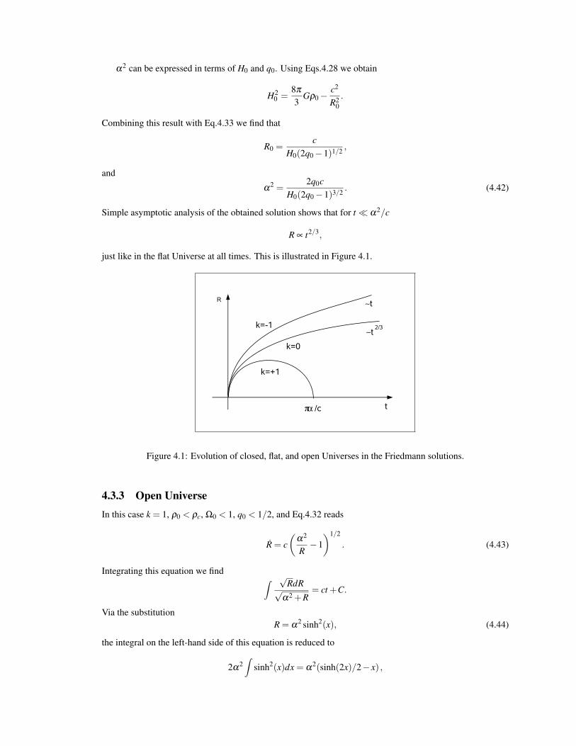
just like in the flat Universe at all times. This is illustrated in Figure 4.1.
R
t
t
t
2/3
k=+1
k=-1
k=0
/c
Figure 4.1: Evolution of closed, flat, and open Universes in the Friedmann solutions.
4.3.3 Open UniverseIn this case k = 1, ρ0 < ρc, Ω0 < 1, q0 < 1/2, and Eq.4.32 reads
R = c(
α2
R−1)1/2
. (4.43)
Integrating this equation we find ∫ √RdR√
α2 +R= ct +C.
Via the substitutionR = α
2 sinh2(x), (4.44)
the integral on the left-hand side of this equation is reduced to
2α2∫
sinh2(x)dx = α2(sinh(2x)/2− x) ,
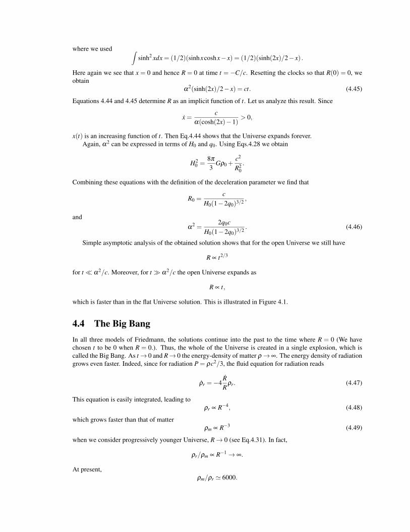
where we used ∫sinh2 xdx = (1/2)(sinhxcoshx− x) = (1/2)(sinh(2x)/2− x) .
Here again we see that x = 0 and hence R = 0 at time t = −C/c. Resetting the clocks so that R(0) = 0, weobtain
α2(sinh(2x)/2− x) = ct. (4.45)
Equations 4.44 and 4.45 determine R as an implicit function of t. Let us analyze this result. Since
x =c
α(cosh(2x)−1)> 0,
x(t) is an increasing function of t. Then Eq.4.44 shows that the Universe expands forever.Again, α2 can be expressed in terms of H0 and q0. Using Eqs.4.28 we obtain
H20 =
8π
3Gρ0 +
c2
R20.
Combining these equations with the definition of the deceleration parameter we find that
R0 =c
H0(1−2q0)3/2 ,
andα
2 =2q0c
H0(1−2q0)3/2 . (4.46)
Simple asymptotic analysis of the obtained solution shows that for the open Universe we still have
R ∝ t2/3
for t α2/c. Moreover, for t α2/c the open Universe expands as
R ∝ t,
which is faster than in the flat Universe solution. This is illustrated in Figure 4.1.
4.4 The Big BangIn all three models of Friedmann, the solutions continue into the past to the time where R = 0 (We havechosen t to be 0 when R = 0.). Thus, the whole of the Universe is created in a single explosion, which iscalled the Big Bang. As t→ 0 and R→ 0 the energy-density of matter ρ→∞. The energy density of radiationgrows even faster. Indeed, since for radiation P = ρc2/3, the fluid equation for radiation reads
ρr =−4RR
ρr. (4.47)
This equation is easily integrated, leading toρr ∝ R−4, (4.48)
which grows faster than that of matterρm ∝ R−3 (4.49)
when we consider progressively younger Universe, R→ 0 (see Eq.4.31). In fact,
ρr/ρm ∝ R−1→ ∞.
At present,ρm/ρr ' 6000.
Thus, we have equipartition, ρm = ρr, when R = Req, where
Req ' R0/6000
and for R < Req the Universe is dominated by radiation. Moreover, the temperature of matter
T ∝Pρ
∝ ρΓ−1 (4.50)
also grows as R→ 0 since Γ> 1. At some point it becomes relativistic and the properties of matter become thesame as those of radiation, with Pm = ρmc2/3. Can the fact that the Universe becomes radiation-dominatedchange the conclusion about the Big Bang? It turns out that it does not. For example consider the case of flatUniverse. Assuming that ρ = ρr the Friedmann equation (Eq.4.28) reads
RR=
aR2 ,
where a is constant. Given the initial condition R(t0) = R0 the solution of this equation is
R2−R20 = 2a(t− t0).
From this result one can see that at finite time
tBB = t0−R2
02a
the scaling factor vanishes,R(tBB) = 0.
Reseting the cosmological time so that tBB = 0, we find
R ∝ t1/2, (4.51)
ρr ∝ R−4 ∝ t−2, (4.52)
ρm ∝ R−3 ∝ t−3/2, (4.53)
H ≡ RR=
12t. (4.54)
(Notice that the Hubble constant is not really a constant – it varies with time!) Thus, the Universe againemerges from a singularity with infinite density and temperature. Immediately after the creation, we cannotpossibly have individual stars or galaxies – all this structure must have been formed much much later. Initially,all there could be is just some very hot “sea” of matter and radiation, dominated by radiation. In fact, closeto the Big Bang the conditions are so extreme that they are beyond the realm of modern Physics, making theFriedmann equations unjustified.
4.5 Advanced topic: Cosmic microwave background radiation
4.5.1 Relic radiationWhen you heat a piece of metal to high temperature it begins to glow, to emit light. In fact, baryonic (orjust normal) matter emits thermal electromagnetic radiation at any temperature, but not always as visiblelight. In fact, higher temperature lead to higher frequency and higher intensity of the thermal emission. Asthe Universe must have been very hot in the past (see Eq.4.50), its matter was producing a lot of radiation.Where is it now? At present, the Universe is transparent to electromagnetic radiation, it is mostly empty.However, the opacity increases with density and in the past the Universe must have been opaque, with photonsbeing absorbed soon after their emission. We should see the photons produced at the time of transition totransparency.
In 1965 two American radio astronomers, Penzias and Wilson, accidently discovered some strange mi-crowave radiation, apparently coming to the Earth from every direction in the sky. Now, this radiation iscalled the cosmic microwave background (CMB) radiation. It has the classical black body thermal spectrumcorresponding to a very low temperature, only ≈ 2.7K. There is no other plausible explanation for it, otherthan cosmological – that this is the radiation left from the early Universe, “the relic radiation”. But why is itstemperature so low if the early Universe was very hot?
4.5.2 Black body spectrum.
By the black body we mean here, we mean a body that does not reflect light. Instead it absorbs andreprocesses any incident electromagnetic radiation. The energy distribution of the black body radiation isgiven by
ε( f ) =8πhc3
f 3
eh f/kT −1, (4.55)
where f is the frequency of radiation, h is the Planck’s constant, k is the Boltzmann constant and T is thetemperature. The meaning of this function is explained by this equation
de = ε( f )dV d f ,
where de is the total energy of photons with the frequencies from f to f +d f within volume dV . That is ε( f )is the radiation energy per unit volume and unit frequency range. The energy of an individual photon withfrequency f is
E = h f (4.56)
Equation 4.55 can be written as
ε( f ) =8πk3T 3
c3h2 F(x) , (4.57)
where x = h f/kT and
F(x) =x3
ex−1.
This function is shown in Figure 4.2. It has a maximum at x ' 2.8, which corresponds to the photon energyE ' 2.8kT . For x 1, F(x) ∝ x2, and for x 1, F(x) ∝ x3e−x.
The number of photons per unit volume and unit frequency range is
n( f ) =ε( f )h f
=8π
c3f 2
eh f/kT −1. (4.58)
Integrating ε( f ) over the whole range of frequencies, which requires a lot of skill, one finds the total energyand mass densities of the radiation
er =
∞∫0
ε( f )d f = arT 4 and ρr = (ar/c2)T 4, (4.59)
where ar = 8π5k4/15h3c3 ' 7.565×10⁻¹⁵ergcm−3K−4 is called the radiation constant. Similarly, one findsthe number density of photons
nr =
∞∫0
n( f )d f = brT 3, (4.60)
where br = 20.3cm−3K−3. The mean energy of photons is
〈E〉= er
nr' 3kT. (4.61)
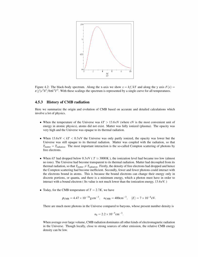
Figure 4.2: The black-body spectrum. Along the x-axis we show x = h f/kT and along the y axis F(x) =ε( f )c3h2/8πk3T 3. With these scalings the spectrum is represented by a single curve for all temperatures.
4.5.3 History of CMB radiation
Here we summarize the origin and evolution of CMB based on accurate and detailed calculations whichinvolve a lot of physics.
• When the temperature of the Universe was kT > 13.6 eV (where eV is the most convenient unit ofenergy in atomic physics), atoms did not exist. Matter was fully ionized (plasma). The opacity wasvery high and the Universe was opaque to its thermal radiation.
• When 13.6eV < kT < 0.3eV the Universe was only partly ionized, the opacity was lower but theUniverse was still opaque to its thermal radiation. Matter was coupled with the radiation, so thatTmatter = Tradiation. The most important interaction is the so-called Compton scattering of photons byfree electrons.
• When kT had dropped below 0.3eV ( T ' 3000K ), the ionization level had became too low (almostno ions). The Universe had become transparent to its thermal radiation. Matter had decoupled from itsthermal radiation, so that Tmatter 6= Tradiation. Firstly, the density of free electrons had dropped and hencethe Compton scattering had become inefficient. Secondly, fewer and fewer photons could interact withthe electrons bound in atoms. This is because the bound electrons can change their energy only indiscrete portions, or quanta, and there is a minimum energy, which a photon must have in order tointeract with a bound electron ( Its value is not much lower than the ionization energy, 13.6eV. )
• Today, for the CMB temperature of T = 2.7K, we have
ρCMB = 4.47×10⁻³⁴gcm−3, nCMB = 400cm−3, 〈E〉= 7×10⁻⁴eV.
There are much more photons in the Universe compared to baryons, whose present number density is
nb = 2.2×10⁻⁵cm−3.
When average over large volume, CMB radiation dominates all other kinds of electromagnetic radiationin the Universe. Though locally, close to strong sources of other emission, the relative CMB energydensity can be low.
4.5.4 Evolution of CMB radiation after decoupling with matterHere we show that in transparent expanding Universe the black body spectrum of CMB is preserved, but at alower temperature. As we have seen in Sec.4.4, for radiation
ρr ∝ R−4.
Since photons are stable particles and do not decay spontaneously their number is conserved and hence
nr ∝ R−3.
Thus, the energy of a single photon
E = h f ∝ρr
nr∝ R−1 and f ∝ R−1. (4.62)
This is exactly the result we have already derived in Eq.4.21. Suppose that at time t = t1 the scale factorR = R1 and the radiation has the black body spectrum
n1( f1, t1) =8π
c3f 21
eh f1/kT1 −1
with temperature T = T1. Consider a small element of the cosmological fluid, expanding with the Universe,Denote as dV1 its volume at time t1. The total number of photons with frequency between f1 and f1 +d f1 inthis volume is
dN = n1( f1, t1)dV1d f1.
As the Universe expands and its scaling factor increases to R2 = αR1 (α > 1), the volume of the fluid elementbecomes
dV2 = dV1α3.
The frequency of photons decreases tof2 = f1/α,
so their move into the frequency “window” d f2 = d f1/α . Thus, the total number of photons within thevolume dV2 and the frequency range ( f2, f2 + d f2) at time t2 is the same it was within the volume dV1 andthe frequency range ( f1, f2 +d f1) at time t1. That is
n1( f1, t1)dV1d f1 = n2( f2, t2)dV2d f2.
Thus,
n2( f2, t2) = n1( f1, t1)dV1
dV2
d f1
d f2= n1( f1, t1)α−2.
The next step is to use the black-body spectrum formula for n1( f1, t1), which gives us
n2( f2) =8π
c3α−2 f 2
1h f1/kT1 −1
=8π
c3f 22
eh f2α/kT1 −1.
This, the black body spectrum for the temperature T2 = T1/α = T1R1/R2. Thus, the black body spectrum ofphotons is preserved, but at a lower temperature, which depends on the scaling factor as
T ∝ R−1. (4.63)
From Eq.4.63, one can conclude that at the time of decoupling the radius of the Universe was
Rdec =2.7
3000R0 ' 10−3R0,
where R0 is its current value. This is about six times larger compared to the scale of the equipartition and,thus, at this point the Universe is already matter-dominated.
4.6 Some other stages of Big Bang
4.6.1 NucleosynthesisThe typical binding energy of complex atomic nuclei is around 1MeV. Thus, in a very hot young Universe,with kT > 1MeV, atomic nuclei could not survive the constant bombardment by extremely energetic particlesand baryons, particles which assemble to make nuclei, were free. As the Universe expanded and cooledto kT 1MeV, nuclei were formed. The detailed analysis of this primordial nucleosynthesis shows thatonly light elements were formed and the early Universe was made mainly of hydrogen. Heavier elements,including carbon, were produced much later by stars.
4.6.2 Structure formationIf soon after Big Bang the Universe was a uniform “sea” of hot plasma then how has all this presently observedstructure, stars, galaxies etc., been formed ? The basic picture is similar to that of the currently observed starformation in the galactic molecular clouds and the key process is the gravitational instability.
Consider the freely expanding Cosmological fluid. There is no gravity force acting on any fluid element.Now imagine that some fluid element is slightly compressed, and hence its mass density is slightly highercompared to its surrounding. The Universe is no longer exactly homogeneous and the gravitational force isno longer vanishing. The fluid element begins to feel its enhanced self-gravity. This force promotes furthercompression leading to even stronger self-gravity and so on. When the fluid is cold this instability alwaysdevelops. However, in hot fluid it is stabilized by the pressure force. As the fluid element gets compressed,its pressure increases and tends to restore the initial volume.
Before the decoupling between matter and radiation in the Universe, the pressure was very high, domi-nated by the radiation pressure Pr = er/3, preventing the development of the gravitational instability. Instead,only sound waves were excited. At the decoupling, the pressure suddenly dropped, as the radiation was nolonger contributing to it. After this, the gravitational instability was winning on many length scales, leadingto the structure we see today.
The spectrum of sound waves generated before the time of decoupling can be determined rather accuratelyusing well known physics. Because of these waves, the Universe was not completely homogeneous at the timeof decoupling and hence the microwave background emission cannot be completely isotropic. Instead, theremust be small fluctuations in its brightness, and hence temperature on the sky. Astronomers were lookingfor such fluctuations for many for years, but all in vain. Only in 1992 they had been finally found with aninstrument on board of the COBE satellite. This was a real triumph of modern Cosmology. The amplitude ofthe fluctuations is very small indeed,
δTT' 10−5,
where T is the temperature.Moreover, the study of the anisotropy has proved to be crucial for determining the geometry of our
Universe. The angular scale of the fluctuations strongly depends on the spatial curvature. The fitting of theobservational data with theoretical models has allowed cosmologists to conclude that within observationalerrors our Universe is flat.
Chapter 5
Measuring the Universe
5.1 Distances to sources with given redshiftIn the case of distant sources, the relation between the source redshift and its distance from us is differentfrom that of Eq.1.2. Consider as an example the case of matter-dominated flat Universe. From the resultsobtained in Sec.4.4 we know that in this case
R(t) = R0
(tt0
)2/3
, (5.1)
where as usual t0 and R0 are the current time and scale factor of the Universe. Combining this result withEq.4.18 we find the time of emission as a function of the redshift
te = t0(1+ z)−3/2. (5.2)
Substituting R(t) from Eq.5.1 into Eq.4.13 and integrating, we find that
χe =3ct2/3
0R0
(t1/30 − t1/3
e ). (5.3)
Next we use the result Eq.5.2 in order to replace te with z and find that
χe =3ct0R0
(1− (1+ z)−1/2). (5.4)
This equations tells us the comoving coordinate of the source with known redshift. In order to find the currentmetric distance to the source, we notice that the distance along the radial direction in flat Universe is simplydl = dr = R0dχ and hence
r(z) = R0χe = 3ct0(1− (1+ z)−1/2). (5.5)
Combining this result with Eq.4.37 for the age of the matter-dominated flat Universe we finally find
r(z) =2cH0
(1− (1+ z)−1/2), (5.6)
which is indeed different from the Hubble law Eq.1.2. However, It is easy to check that the Hubble law isrecovered from this result in the limit z 1. Indeed, using the first two terms of Taylor’s expansion we obtain
(1− (1+ z)−1/2)∼ 1− (1− (1/2)z) = (1/2)z,
and thusr(z)∼ c
H0z . (5.7)
45
5.2 The cosmological horizonThe Universe may be finite or infinite but can we actually verify this? How far can we “see”? Or to be moreaccurate, how far are the objects in the Universe which have had enough time since the birth of the Universeto communicate their presence to us, at least in principle? In order to answer this question, or even to seeif this question makes sense, we need to find out is how far the fastest possible signal can reach since theBig Bang. Obviously, this has to be a signal propagating with the speed of light along a “straight line” ( ageodesic to be more accurate). In fact, we have already derived the required equation – this is Eq.4.13 withte = 0
t∫0
cdtR(t)
=
χh∫0
dχ√1− kχ2
. (5.8)
Indeed, this equation defines the comoving radial coordinate χh(t) at time t of the signal that was produced attime t = 0 at the origin of the coordinate grid. Obviously, the result depends on the geometry of the Universe,which we need to know in order to evaluate the integral on the right hand side of Eq.5.8, and on the historyof the Universe, as we need to know R(t) as well.
Consider, as an example, the model of flat matter-dominated Universe. Since k = 0, we have
χh∫0
dχ√1− kχ2
= χ .
In addition,R(t) = At2/3 (5.9)
(see Sec.4.4), which leads to
t0∫0
cdtR(t)
=3cA
t1/3 . (5.10)
Thus, we have
χh(t) =3cA
t1/3. (5.11)
This result shows that we can explore only a finite part of the Universe. The rest is, so to speak, beyond the“horizon”. This is why χh(t) is called the comoving radius of the cosmological horizon. As the Universe getsolder, the horizon expands, allowing us to see more of the Universe. However, this is still only an insignificantfraction as the Universe is infinite. The metric radius of the horizon in this model is
rh(t) = R(t)χh(t) = 3ct . (5.12)
At first glance this result appears rather odd as rh is larger than the speed of light times the propagationtime, which seems to be in conflict with the Theory of Relativity. However, there is no conflict. Indeed, asthe signal propagates the length of any given section of the path it has already made increases due to theexpansion of the Universe.
In order to convert χh(t) into rh(t) for other models, we note that along the path of the signal both θ andφ are constant, and hence the line element of this path is
dl = R(t)dχ√
1− kχ2. (5.13)
Thus,
rh(t) = R(t)
χh(t)∫0
dχ√1− kχ2
. (5.14)
For the closed Universe ( k = 1 )rh(t) = R(t)sin−1(χh(t)) ; (5.15)
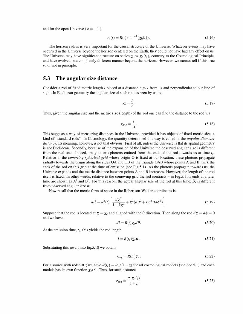
and for the open Universe ( k =−1 )
rh(t) = R(t)sinh−1(χh(t)) . (5.16)
The horizon radius is very important for the causal structure of the Universe. Whatever events may haveoccurred in the Universe beyond the horizon centered on the Earth, they could not have had any effect on us.The Universe may have significant structure on scales χ χh(t0), contrary to the Cosmological Principle,and have evolved in a completely different manner beyond the horizon. However, we cannot tell if this trueso or not in principle.
5.3 The angular size distanceConsider a rod of fixed metric length l placed at a distance r l from us and perpendicular to our line ofsight. In Euclidean geometry the angular size of such rod, as seen by us, is
α =lr. (5.17)
Thus, given the angular size and the metric size (length) of the rod one can find the distance to the rod via
rang =lα. (5.18)
This suggests a way of measuring distances in the Universe, provided it has objects of fixed metric size, akind of “standard rods”. In Cosmology, the quantity determined this way is called in the angular diameterdistance. Its meaning, however, is not that obvious. First of all, unless the Universe is flat its spatial geometryis not Euclidean. Secondly, because of the expansion of the Universe the observed angular size is differentfrom the real one. Indeed, imagine two photons emitted from the ends of the rod towards us at time te.Relative to the comoving spherical grid whose origin O is fixed at our location, these photons propagateradially towards the origin along the sides OA and OB of the triangle OAB whose points A and B mark theends of the rod on this grid at the time of emission (see Fig.5.1). As the photons propagate towards us, theUniverse expands and the metric distance between points A and B increases. However, the length of the roditself is fixed. In other words, relative to the comoving grid the rod contracts – in Fig.5.1 its ends at a latertime are shown as A′ and B′. For this reason, the actual angular size of the rod at this time, β , is differentfrom observed angular size α .
Now recall that the metric form of space in the Robertson-Walker coordinates is
dl2 = R2(t)[
dχ2
1− kχ2 +χ2(dθ
2 + sin2θdφ
2)
]. (5.19)
Suppose that the rod is located at χ = χe and aligned with the θ direction. Then along the rod dχ = dφ = 0and we have
dl = R(t)χedθ . (5.20)
At the emission time, te, this yields the rod length
l = R(te)χeα. (5.21)
Substituting this result into Eq.5.18 we obtain
rang = R(te)χe . (5.22)
For a source with redshift z we have R(te) = R0/(1+ z) for all cosmological models (see Sec.5.1) and eachmodels has its own function χe(z). Thus, for such a source
rang =R0χe(z)
1+ z. (5.23)
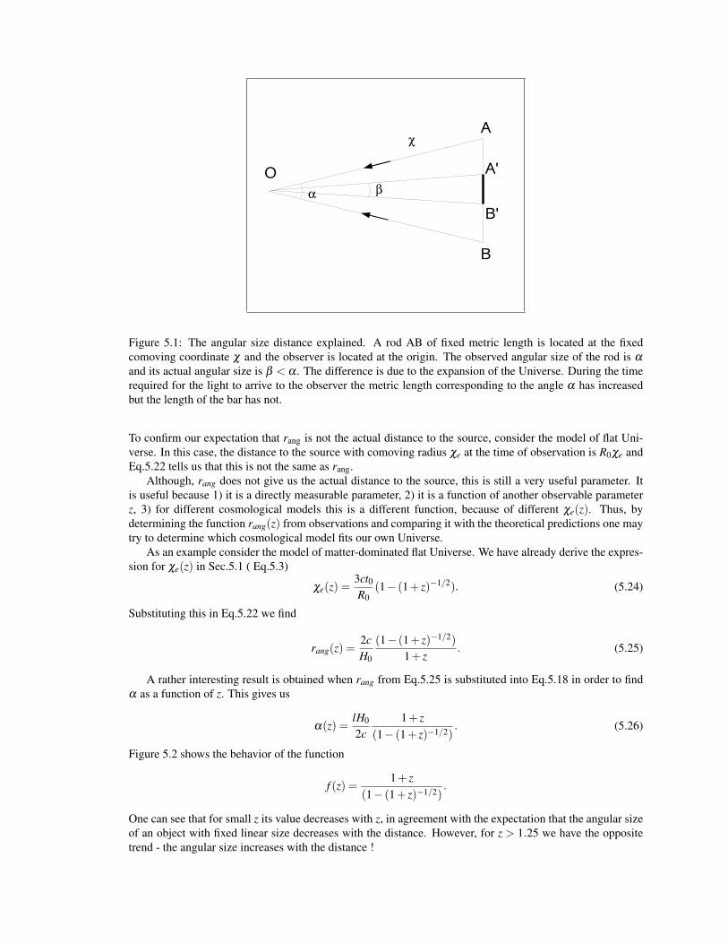
A
B
A'
B'
O
Figure 5.1: The angular size distance explained. A rod AB of fixed metric length is located at the fixedcomoving coordinate χ and the observer is located at the origin. The observed angular size of the rod is α
and its actual angular size is β < α . The difference is due to the expansion of the Universe. During the timerequired for the light to arrive to the observer the metric length corresponding to the angle α has increasedbut the length of the bar has not.
To confirm our expectation that rang is not the actual distance to the source, consider the model of flat Uni-verse. In this case, the distance to the source with comoving radius χe at the time of observation is R0χe andEq.5.22 tells us that this is not the same as rang.
Although, rang does not give us the actual distance to the source, this is still a very useful parameter. Itis useful because 1) it is a directly measurable parameter, 2) it is a function of another observable parameterz, 3) for different cosmological models this is a different function, because of different χe(z). Thus, bydetermining the function rang(z) from observations and comparing it with the theoretical predictions one maytry to determine which cosmological model fits our own Universe.
As an example consider the model of matter-dominated flat Universe. We have already derive the expres-sion for χe(z) in Sec.5.1 ( Eq.5.3)
χe(z) =3ct0R0
(1− (1+ z)−1/2). (5.24)
Substituting this in Eq.5.22 we find
rang(z) =2cH0
(1− (1+ z)−1/2)
1+ z. (5.25)
A rather interesting result is obtained when rang from Eq.5.25 is substituted into Eq.5.18 in order to findα as a function of z. This gives us
α(z) =lH0
2c1+ z
(1− (1+ z)−1/2). (5.26)
Figure 5.2 shows the behavior of the function
f (z) =1+ z
(1− (1+ z)−1/2).
One can see that for small z its value decreases with z, in agreement with the expectation that the angular sizeof an object with fixed linear size decreases with the distance. However, for z > 1.25 we have the oppositetrend - the angular size increases with the distance !
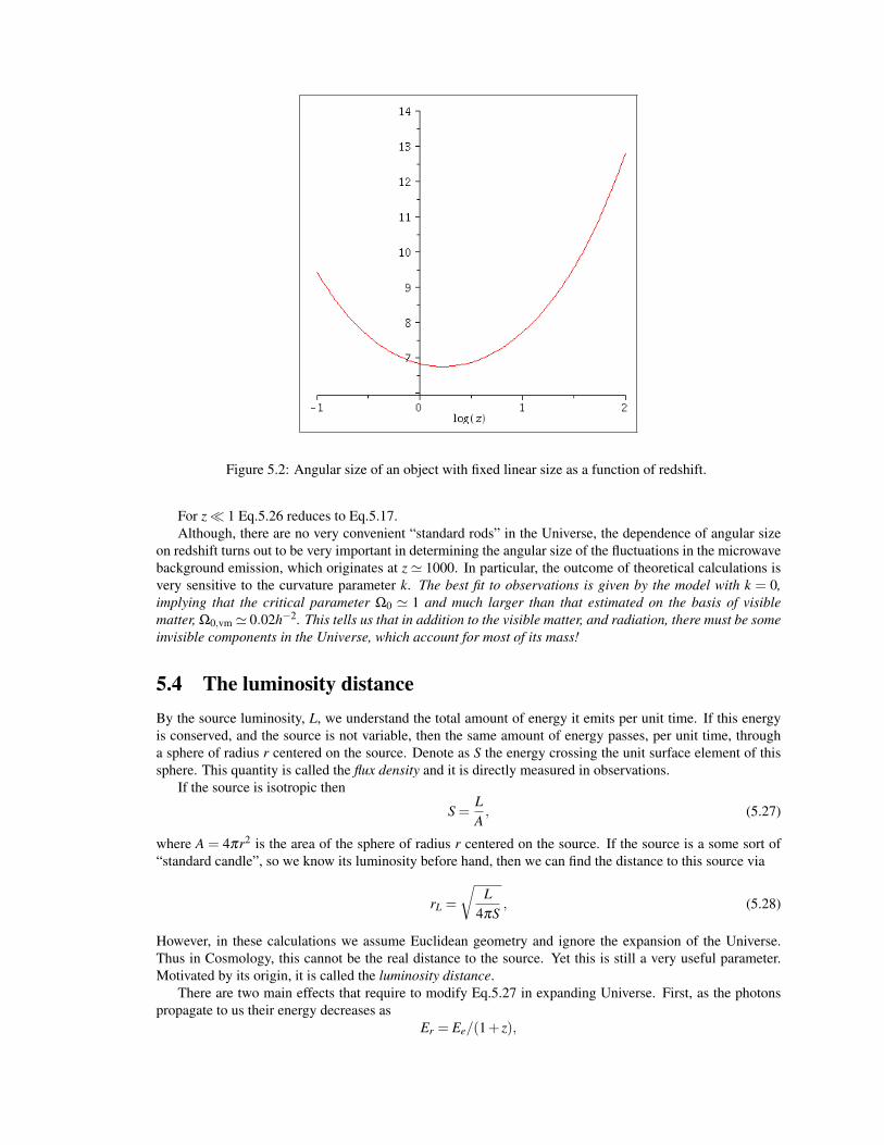
Figure 5.2: Angular size of an object with fixed linear size as a function of redshift.
For z 1 Eq.5.26 reduces to Eq.5.17.Although, there are no very convenient “standard rods” in the Universe, the dependence of angular size
on redshift turns out to be very important in determining the angular size of the fluctuations in the microwavebackground emission, which originates at z ' 1000. In particular, the outcome of theoretical calculations isvery sensitive to the curvature parameter k. The best fit to observations is given by the model with k = 0,implying that the critical parameter Ω0 ' 1 and much larger than that estimated on the basis of visiblematter, Ω0,vm ' 0.02h−2. This tells us that in addition to the visible matter, and radiation, there must be someinvisible components in the Universe, which account for most of its mass!
5.4 The luminosity distanceBy the source luminosity, L, we understand the total amount of energy it emits per unit time. If this energyis conserved, and the source is not variable, then the same amount of energy passes, per unit time, througha sphere of radius r centered on the source. Denote as S the energy crossing the unit surface element of thissphere. This quantity is called the flux density and it is directly measured in observations.
If the source is isotropic then
S =LA, (5.27)
where A = 4πr2 is the area of the sphere of radius r centered on the source. If the source is a some sort of“standard candle”, so we know its luminosity before hand, then we can find the distance to this source via
rL =
√L
4πS, (5.28)
However, in these calculations we assume Euclidean geometry and ignore the expansion of the Universe.Thus in Cosmology, this cannot be the real distance to the source. Yet this is still a very useful parameter.Motivated by its origin, it is called the luminosity distance.
There are two main effects that require to modify Eq.5.27 in expanding Universe. First, as the photonspropagate to us their energy decreases as
Er = Ee/(1+ z),
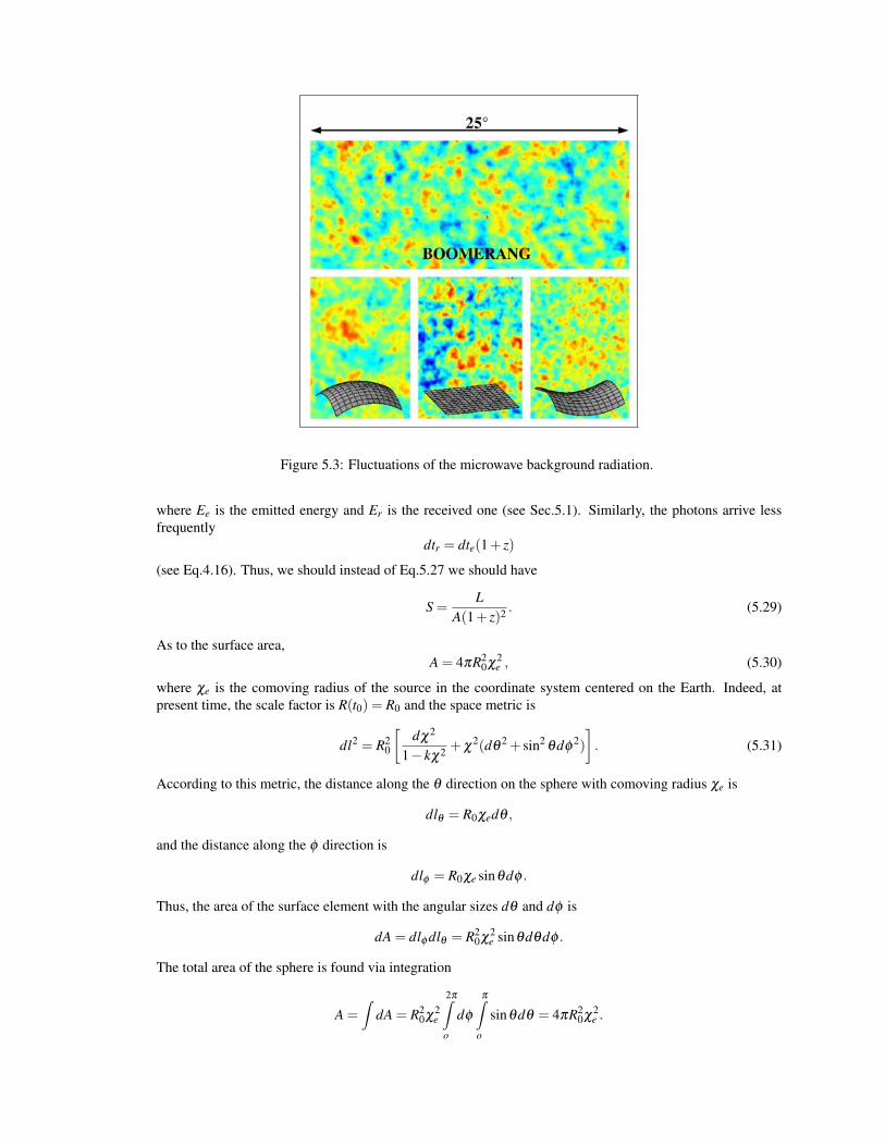
Figure 5.3: Fluctuations of the microwave background radiation.
where Ee is the emitted energy and Er is the received one (see Sec.5.1). Similarly, the photons arrive lessfrequently
dtr = dte(1+ z)
(see Eq.4.16). Thus, we should instead of Eq.5.27 we should have
S =L
A(1+ z)2 . (5.29)
As to the surface area,A = 4πR2
0χ2e , (5.30)
where χe is the comoving radius of the source in the coordinate system centered on the Earth. Indeed, atpresent time, the scale factor is R(t0) = R0 and the space metric is
dl2 = R20
[dχ2
1− kχ2 +χ2(dθ
2 + sin2θdφ
2)
]. (5.31)
According to this metric, the distance along the θ direction on the sphere with comoving radius χe is
dlθ = R0χedθ ,
and the distance along the φ direction is
dlφ = R0χe sinθdφ .
Thus, the area of the surface element with the angular sizes dθ and dφ is
dA = dlφ dlθ = R20χ
2e sinθdθdφ .
The total area of the sphere is found via integration
A =∫
dA = R20χ
2e
2π∫o
dφ
π∫o
sinθdθ = 4πR20χ
2e .
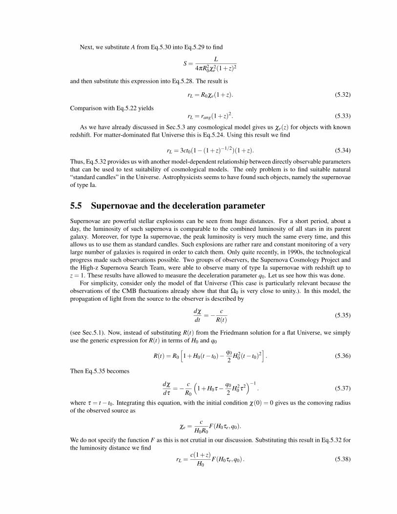
Next, we substitute A from Eq.5.30 into Eq.5.29 to find
S =L
4πR20χ2
e (1+ z)2
and then substitute this expression into Eq.5.28. The result is
rL = R0χe(1+ z). (5.32)
Comparison with Eq.5.22 yieldsrL = rang(1+ z)2. (5.33)
As we have already discussed in Sec.5.3 any cosmological model gives us χe(z) for objects with knownredshift. For matter-dominated flat Universe this is Eq.5.24. Using this result we find
rL = 3ct0(1− (1+ z)−1/2)(1+ z). (5.34)
Thus, Eq.5.32 provides us with another model-dependent relationship between directly observable parametersthat can be used to test suitability of cosmological models. The only problem is to find suitable natural“standard candles” in the Universe. Astrophysicists seems to have found such objects, namely the supernovaeof type Ia.
5.5 Supernovae and the deceleration parameterSupernovae are powerful stellar explosions can be seen from huge distances. For a short period, about aday, the luminosity of such supernova is comparable to the combined luminosity of all stars in its parentgalaxy. Moreover, for type Ia supernovae, the peak luminosity is very much the same every time, and thisallows us to use them as standard candles. Such explosions are rather rare and constant monitoring of a verylarge number of galaxies is required in order to catch them. Only quite recently, in 1990s, the technologicalprogress made such observations possible. Two groups of observers, the Supernova Cosmology Project andthe High-z Supernova Search Team, were able to observe many of type Ia supernovae with redshift up toz = 1. These results have allowed to measure the deceleration parameter q0. Let us see how this was done.
For simplicity, consider only the model of flat Universe (This case is particularly relevant because theobservations of the CMB fluctuations already show that that Ω0 is very close to unity.). In this model, thepropagation of light from the source to the observer is described by
dχ
dt=− c
R(t)(5.35)
(see Sec.5.1). Now, instead of substituting R(t) from the Friedmann solution for a flat Universe, we simplyuse the generic expression for R(t) in terms of H0 and q0
R(t) = R0
[1+H0(t− t0)−
q0
2H2
0 (t− t0)2]. (5.36)
Then Eq.5.35 becomes
dχ
dτ=− c
R0
(1+H0τ− q0
2H2
0 τ2)−1
. (5.37)
where τ = t− t0. Integrating this equation, with the initial condition χ(0) = 0 gives us the comoving radiusof the observed source as
χe =c
H0R0F(H0τe,q0).
We do not specify the function F as this is not crutial in our discussion. Substituting this result in Eq.5.32 forthe luminosity distance we find
rL =c(1+ z)
H0F(H0τe,q0) . (5.38)
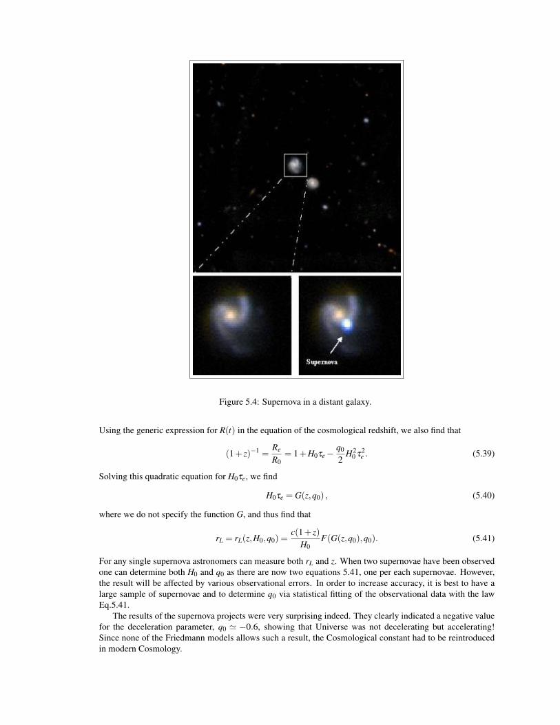
Figure 5.4: Supernova in a distant galaxy.
Using the generic expression for R(t) in the equation of the cosmological redshift, we also find that
(1+ z)−1 =Re
R0= 1+H0τe−
q0
2H2
0 τ2e . (5.39)
Solving this quadratic equation for H0τe, we find
H0τe = G(z,q0) , (5.40)
where we do not specify the function G, and thus find that
rL = rL(z,H0,q0) =c(1+ z)
H0F(G(z,q0),q0). (5.41)
For any single supernova astronomers can measure both rL and z. When two supernovae have been observedone can determine both H0 and q0 as there are now two equations 5.41, one per each supernovae. However,the result will be affected by various observational errors. In order to increase accuracy, it is best to have alarge sample of supernovae and to determine q0 via statistical fitting of the observational data with the lawEq.5.41.
The results of the supernova projects were very surprising indeed. They clearly indicated a negative valuefor the deceleration parameter, q0 ' −0.6, showing that Universe was not decelerating but accelerating!Since none of the Friedmann models allows such a result, the Cosmological constant had to be reintroducedin modern Cosmology.
Chapter 6
Secret components of the Universe
As this has been noted in Sec.5.3, the observed fluctuations of the Cosmic microwave background radiationimply that the density parameter is very close to unity
Ω0 ' 1,
and the question arises if this result is consistent with the astronomical observations. Indeed, these observa-tions allows us to measure the local density of the Universe directly.
6.1 Dark MatterIn galaxies, most of the visible mass is present in the form of stars. Many researchers looked into the issueof stellar contribution to the density parameter. They converged to the conclusion that it is very small,Ω0,stars = ρstars/ρc ' 0.01 . Spiral galaxies also have a substantial mass in the form of interstellar gas butthis is still smaller compared to their stellar mass. A substantial amount of gas is also present in clusters ofgalaxies, the intergalactic gas, where its total mass can even exceed the stellar mass but not by much. In total,the visible matter in the Universe can only yield
Ω0,vm = 0.05 . (6.1)
If there is a massive invisible material component, the so-called dark matter, in the Universe then its pres-ence will be felt by visible matter via the gravitational field of the dark matter. In particular the characteristicspeeds of stars in galaxies, and galaxies in clusters of galaxies will be higher than expected. The gravity ofthis dark matter will also effect the quasi-hydrostatic equilibrium of the gaseous components. This is indeedwhat is observed.
In particular, the rotation of spiral galaxies is too fast to be explained by the gravity of the visible compo-nent alone. In fact, the motion of individual stars in galaxies is very accurately described by the Newtoniantheory. According to this theory the centrifugal acceleration is provided by the gravitational pull so that
v2
r=
GM(r)r2 , (6.2)
where v is the orbital velocity, r is the distance from the center of the galaxy, and M(r) is the total masscontained within sphere of radius r (see Sec.8.1). Thus by measuring the orbital motion of its stars, onecan determine the distribution of mass in the galaxy. Studies conducted along these lines have concludedthat galaxies must contain invisible matter in the form of extended and more or less spherical halos (seeFig.6.1). Moreover, its mass exceeds that of visible matter by a factor ranging from five to ten. Yet, thedensity parameter due to the contribution of dark galactic halos is still much lower then unity,
Ω0,halo ' 0.1 .
Similar studies, where individual galaxies played the role of test particles, have deduced the presence ofmassive invisible component on the scale of galactic clusters. In fact, there are other methods that can be
53
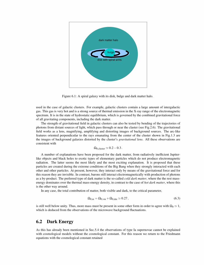
bulge
disk with spiral arms
dark matter halo
Figure 6.1: A spiral galaxy with its disk, bulge and dark matter halo.
used in the case of galactic clusters. For example, galactic clusters contain a large amount of intergalacticgas. This gas is very hot and is a strong source of thermal emission in the X-ray range of the electromagneticspectrum. It is in the state of hydrostatic equilibrium, which is governed by the combined gravitational forceof all gravitating components, including the dark matter.
The strength of gravitational field in galactic clusters can also be tested by bending of the trajectories ofphotons from distant sources of light, which pass through or near the claster (see Fig.2.6). The gravitationalfield works as a lens, magnifying, amplifying and distorting images of background sources. The arc-likefeatures oriented perpendicular to the rays emanating from the center of the cluster shown in Fig.1.3 arethe images of background galaxies distorted by the cluster’s gravitational lens. All these observations areconsistent with
Ω0,cluster ' 0.2−0.3 .
A number of explanations have been proposed for the dark matter, from radiatively inefficient Jupiter-like objects and black holes to exotic types of elementary particles which do not produce electromagneticradiation. The latter seems the most likely and the most exciting explanation. It is proposed that theseparticles are created during the extreme conditions of the Big Bang when they strongly interacted with eachother and other particles. At present, however, they interact only by means of the gravitational force and forthis reason they are invisible. In contrast, barons still interact electromagnetically with production of photonsas a by-product. The preferred type of dark matter is the so-called cold dark matter, where the the rest mass-energy dominates over the thermal mass-energy density, in contrast to the case of hot dark matter, where thisis the other way around.
In any case, the total contribution of matter, both visible and dark, to the critical parameter,
Ω0,m = Ω0,vm +Ω0,dm ' 0.27 , (6.3)
is still well below unity. Thus, more mass must be present in some other form in order to agree with Ω0 ' 1,which is deduced from the observations of the microwave background fluctuations.
6.2 Dark EnergyAs this has already been mentioned in Sec.5.4 the observations of type Ia supernovae cannot be explainedwith cosmological models without the cosmological constant. For this reason we return to the Friedmannequations with the cosmological constant retained
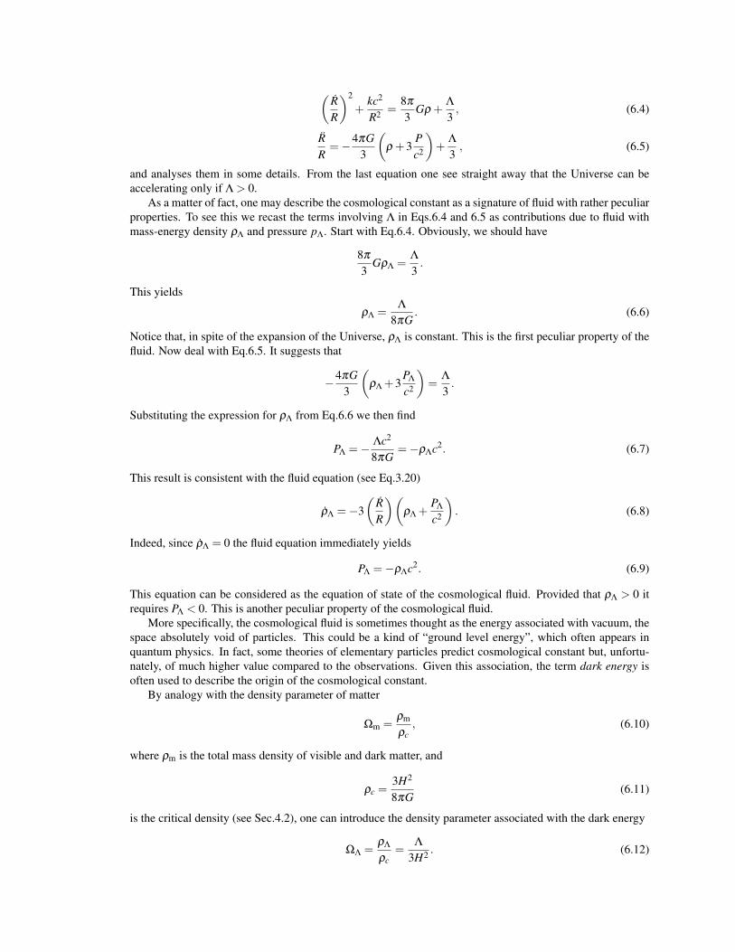
(RR
)2
+kc2
R2 =8π
3Gρ +
Λ3, (6.4)
RR=−4πG
3
(ρ +3
Pc2
)+
Λ3, (6.5)
and analyses them in some details. From the last equation one see straight away that the Universe can beaccelerating only if Λ > 0.
As a matter of fact, one may describe the cosmological constant as a signature of fluid with rather peculiarproperties. To see this we recast the terms involving Λ in Eqs.6.4 and 6.5 as contributions due to fluid withmass-energy density ρΛ and pressure pΛ. Start with Eq.6.4. Obviously, we should have
8π
3GρΛ =
Λ3.
This yields
ρΛ =Λ
8πG. (6.6)
Notice that, in spite of the expansion of the Universe, ρΛ is constant. This is the first peculiar property of thefluid. Now deal with Eq.6.5. It suggests that
−4πG3
(ρΛ +3
PΛc2
)=
Λ3.
Substituting the expression for ρΛ from Eq.6.6 we then find
PΛ =− Λc2
8πG=−ρΛc2. (6.7)
This result is consistent with the fluid equation (see Eq.3.20)
ρΛ =−3(
RR
)(ρΛ +
PΛc2
). (6.8)
Indeed, since ρΛ = 0 the fluid equation immediately yields
PΛ =−ρΛc2. (6.9)
This equation can be considered as the equation of state of the cosmological fluid. Provided that ρΛ > 0 itrequires PΛ < 0. This is another peculiar property of the cosmological fluid.
More specifically, the cosmological fluid is sometimes thought as the energy associated with vacuum, thespace absolutely void of particles. This could be a kind of “ground level energy”, which often appears inquantum physics. In fact, some theories of elementary particles predict cosmological constant but, unfortu-nately, of much higher value compared to the observations. Given this association, the term dark energy isoften used to describe the origin of the cosmological constant.
By analogy with the density parameter of matter
Ωm =ρm
ρc, (6.10)
where ρm is the total mass density of visible and dark matter, and
ρc =3H2
8πG(6.11)
is the critical density (see Sec.4.2), one can introduce the density parameter associated with the dark energy
ΩΛ =ρΛρc
=Λ
3H2 . (6.12)
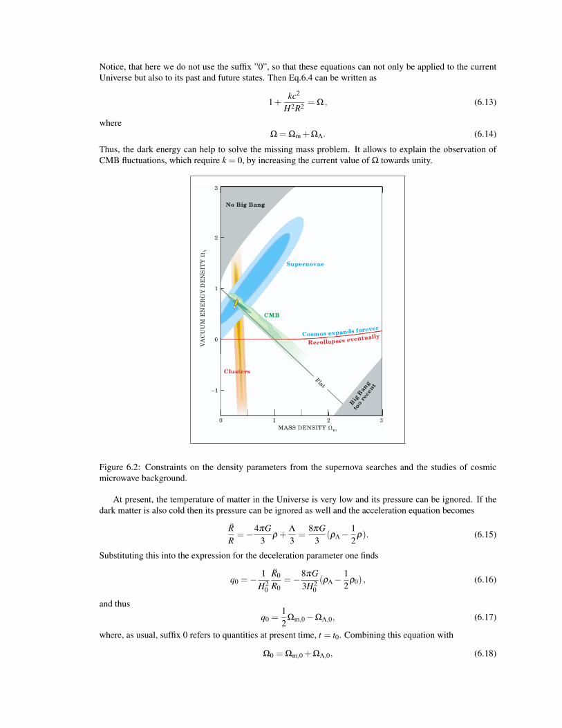
Notice, that here we do not use the suffix ”0”, so that these equations can not only be applied to the currentUniverse but also to its past and future states. Then Eq.6.4 can be written as
1+kc2
H2R2 = Ω , (6.13)
whereΩ = Ωm +ΩΛ. (6.14)
Thus, the dark energy can help to solve the missing mass problem. It allows to explain the observation ofCMB fluctuations, which require k = 0, by increasing the current value of Ω towards unity.
Figure 6.2: Constraints on the density parameters from the supernova searches and the studies of cosmicmicrowave background.
At present, the temperature of matter in the Universe is very low and its pressure can be ignored. If thedark matter is also cold then its pressure can be ignored as well and the acceleration equation becomes
RR=−4πG
3ρ +
Λ3=
8πG3
(ρΛ−12
ρ). (6.15)
Substituting this into the expression for the deceleration parameter one finds
q0 =−1
H20
R0
R0=−8πG
3H20(ρΛ−
12
ρ0) , (6.16)
and thusq0 =
12
Ωm,0−ΩΛ,0, (6.17)
where, as usual, suffix 0 refers to quantities at present time, t = t0. Combining this equation with
Ω0 = Ωm,0 +ΩΛ,0, (6.18)
we find thatΩΛ,0 =
13
Ω0−23
q0 (6.19)
andΩm,0 =
23
Ω0 +23
q0 . (6.20)
Thus, the observational data on q0 and Ω0 can be used to find the values of Ωm,0 and ΩΛ,0. The current datashow that
Ωm,0 ' 0.27 and ΩΛ,0 ' 0.73
(see Figure 6.2). This value of Ωm,0 agrees very well with the astronomical observations of the local Universe.

Chapter 7
The phase of inflation
7.1 The problems of Friedmann CosmologyThere are a number of puzzling issues in the Friedmann Cosmology. Here we discuss only two of them,the flatness problem and the horizon problem. Other issues are a bit more complex and require a very goodbackground in physics.
7.1.1 The flatness problemAccording to the cosmological observations, the critical parameter is very close to unity. Why is this? Unlessthe Universe is exactly flat ( k = 0 ), we should have Ω 6= 1. What was the value of Ω in the past? Could ithave evolved naturally towards unity when the Universe was very young? If it could then this observationalresult would have a simple explanation. If not, then this becomes a mystery.
From Eq.6.13 we have
|1−Ω|= |k|c2
H2R2 . (7.1)
Thus, the evolution of Ω is determined by the evolution of HR.For a young Universe, both the curvature term and the cosmological terms in the Friedmann equations
can be ignored. Indeed, Λ is constant, whereas ρ evolves as R−3 in a matter-dominated Universe, and as R−4
in a radiation dominated Universe. Thus, for small R the Friedmann equation(RR
)2
+kc2
R2 =8π
3Gρ +
Λ3
(7.2)
reduces to (RR
)2
+kc2
R2 =8π
3Gρ. (7.3)
The curvature term grows only as R−2 when R decreases and therefore for sufficiently small R it also becomessmall compared to the matter/radiation term (the term on the right-hand side of this equation). Thus, theFriedmann equation for a young Universe is very simple(
RR
)2
=8π
3Gρ. (7.4)
Finally, since ρradiation/ρmatter ∝ R−1, we may focus only on the case of radiation-dominated Universe, forwhich this equation gives the solution
R ∝ t1/2 and HR ∝ t−1/2. (7.5)
Substituting this result into Eq.7.1 we find that
|1−Ω| ∝ t. (7.6)
59
Thus, Ω does not evolve naturally towards unity as the Universe expands. On the contrary, it moves awayfrom it and in order to have Ω0 ' 1 at present, Ω has to be extremely close to unity in the past. This is theflatness problem of Big Bang Cosmology.
7.1.2 The horizon problemWhy is the Universe uniform? Is there a natural explanation to this, hinted by the Friedmann solutions?Well, the uniformity could imply an efficient mechanism of erasing inhomogeneities in the early Universe.However, no matter what actual physical processes are involved in this, in order for them to work an effectivecommunication between different parts of the now observable Universe must have existed in the past.
In order to see this, consider a box, which has been filled with gas through a number of holes in its walls.Given time, the gas distribution in the box becomes uniform. It is the gas pressure which becomes uniformfirst and this process involves sound waves crossing the box from one end to another, back and forward.For the density to become uniform even more time is required because this involves slower processes, likediffusion and thermal conductivity. Thus, the time, which is required to reach a uniform state in the box islarger than the sound wave crossing time of the box. Since no wave can propagate faster than light, the lightcrossing time sets the lowest possible limit on the time of settling to a uniform state.
At present, we can observe the Universe up to the CMB sphere, beyond which the Universe is not trans-parent to the electromagnetic radiation (light). The CMB photons, which are reaching the Earth now, wereproduced at this sphere at the time of decoupling of matter and radiation. With time, the comoving radius ofthe CMB sphere increases, and larger part of the Universe becomes accessible to observational studies. Thesize of causally connected regions of the Universe is given by the radius of the cosmological horizon ( seeSec.5.2 ). The fact that there are no significant variations of the CMB emission in the sky means that thecomoving radius of the horizon at the time of decoupling was much larger compared to the current comovingradius of the CMB sphere.
One can formulate this condition in terms of metric radii rather than the comoving ones, which is in facta bit more convenient. For this we simply need to convert the comoving radii into the metric ones using thesame value of the scaling factor. For example, we may use the scaling factor at the time of decoupling. Thiswill give us the metric radius of the horizon at the time of decoupling and the metric radius which the currentCMB sphere had at that time. The isotropy of CMB requires the horizon radius to be much larger. It turnsout that this is in conflict with the Friedmann models.
The comoving radius of the cosmological horizon χh(t) is given by the equation
t∫0
cdtR(t)
=
χh(t)∫0
dχ√1− kχ2
(7.7)
( see Sec.5.2 ). The corresponding metric radius at this time is
rh(t) = R(t)
χh(t)∫0
dχ√1− kχ2
(7.8)
Thus, we havet∫
0
cdtR(t)
=rh(t)R(t)
. (7.9)
Both the matter-dominated and the radiation-dominated solutions of the Friedmann equations give
R(t)' R0
(tt0
)α
, (7.10)
with 1/2 < α < 2/3. This is because α = 2/3 for the matter-dominated model and α = 1/2 for the radiation-dominated model. In this case
H(t) =RR=
α
t. (7.11)
Substituting R(t) from Eq.7.10 into the left-hand side of Eq.7.9 and integrating, one finds that
rh(t) =ct
1−α=
(α
α−1
)c
H(t)' c
H(t). (7.12)
Thus, at the time of decouplingrh(tdec)'
cH(tdec)
. (7.13)
The current comoving radius of the CMB sphere, χCMB, is given by
t0∫tdec
cdtR(t)
=
χCMB∫0
dχ√1− kχ2
. (7.14)
The corresponding metric radius at the time of decoupling is
rCMB(tdec) = R(tdec)
χCMB∫0
dχ√1− kχ2
. (7.15)
Thus, we havet0∫
tdec
cdtR(t)
=rCMB(tdec)
R(tdec). (7.16)
Substituting into this equation R(t) from Eq.7.10 and integrating, we obtain
rCMB(tdec) =α
α−1R(tdec)
R0
cH0' R(tdec)
R0
cH0
. (7.17)
Thus,rh
rCMB(tdec)' R0
R(tdec)
H0
H(tdec). (7.18)
Using Eqs.7.10 and 7.11H0
H(tdec)=
tdec
t0=
(R(tdec)
R0
)1/α
and we finally obtainrh
rCMB(tdec)'(
R(tdec)
R0
)1/α−1
1 (7.19)
because R(tdec) R0 ( see Sec.4.5). Thus, the observed CMB radiation is produced by causally disconnectedparts of the Universe! This means that the observed uniformity of the Universe cannot be established naturallyin the Friedmann cosmology! This result is known as the horizon problem.
7.2 InflationAccording to the Friedmann equation, (
RR
)2
+kc2
R2 =8π
3Gρ +
Λ3, (7.20)
the dynamics of the Universe will eventually be dominated by Cosmological constant. Indeed, both thecurvature and the matter/radiation terms decrease with R, whereas the cosmological constant term remainsconstant. In this limit (
RR
)2
=Λ3, (7.21)
which yields the solution
R = Aexp
(√Λ3
t
), (7.22)
where A is the constant of integration. Thus, the Universe expands exponentially.What is the evolution of the critical parameter during this expansion? The Hubble constant
H =R(t)R(t)
=
√Λ3
(7.23)
is constant, and
HR ∝ exp
(√Λ3
t
).
This implies that
|1−Ω|= |k|c2
H2R2 ∝ exp
(−2
√Λ3
t
). (7.24)
Thus, Ω is driven towards unity. This analysis suggests that the flatness problem of the Friedmann Cosmologycan be solved if soon after the Big Bang instead of the usual matter and radiation the Universe was filled witha “fluid” similar to the one associated with the Cosmological constant (see Sec.6.2). The corresponding phaseof exponential expansion is called the inflation. At the end of this phase, a some kind of phase transition takesplace, where this hypothetical exotic fluid is transformed into the usual mixture of radiation and matter.
What is about the horizon problem? First, we notice that from Eq.7.22 R(t)→ 0 only as t→−∞, implyinginfinitely long phase of inflation. If the lifetime of the Universe is in fact finite, then the phase of inflationhad a beginning, where it replaced some other previous phase in the evolution of the Universe. Without lossof generality we may put t = 0 at the start of the inflation. Assuming that the horizon radius at this point wassmall, χh(0)' 0, we may compute its further evolution via
t∫0
cdtR
=
χh∫0
dχ√1− kχ2
=rh
R(7.25)
as before (see Eq.7.9). Substituting into the left-hand side of this equation R(t) from Eq.7.22 and integratingwe obtain
rh = RcA
√3Λ
[1− exp(−
√Λ3
t)
]. (7.26)
For t√
3/Λ this gives us
rh = RcA
√3Λ
=cH
exp(
√Λ3
t) cH
. (7.27)
Comparing this result with Eq.7.12 we can see that the radius of the cosmological horizon at the end ofinflation can easily exceed that of standard Friedmann cosmology by many orders of magnitude and hencecan easily exceed the radius of the CMB sphere at the time of decoupling. This is simply because the Universeexpands very slowly during the inflation, whereas the cosmological horizon keeps expanding with the speedof light as before. As the result it encloses much larger volume of the Universe.
The theory of inflation successfully resolves many other problems of the Friedmann Cosmology, whichwe can not discuss within the limited scope of this module. In fact it remains a very hot topical issue inmodern Cosmology.
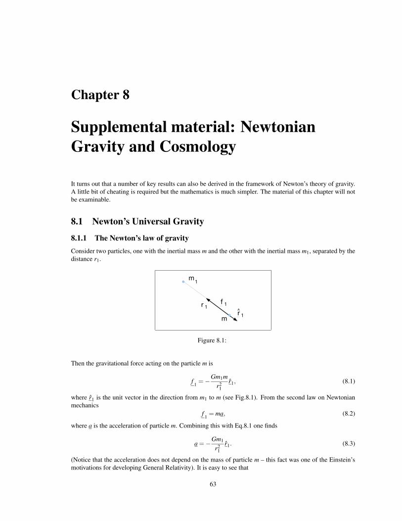
Chapter 8
Supplemental material: NewtonianGravity and Cosmology
It turns out that a number of key results can also be derived in the framework of Newton’s theory of gravity.A little bit of cheating is required but the mathematics is much simpler. The material of this chapter will notbe examinable.
8.1 Newton’s Universal Gravity
8.1.1 The Newton’s law of gravityConsider two particles, one with the inertial mass m and the other with the inertial mass m1, separated by thedistance r1.
m
m1
f 1r 1
r 1^
Figure 8.1:
Then the gravitational force acting on the particle m is
f1=−Gm1m
r21
r1, (8.1)
where r1 is the unit vector in the direction from m1 to m (see Fig.8.1). From the second law on Newtonianmechanics
f1= ma, (8.2)
where a is the acceleration of particle m. Combining this with Eq.8.1 one finds
a =−Gm1
r21
r1. (8.3)
(Notice that the acceleration does not depend on the mass of particle m – this fact was one of the Einstein’smotivations for developing General Relativity). It is easy to see that
63
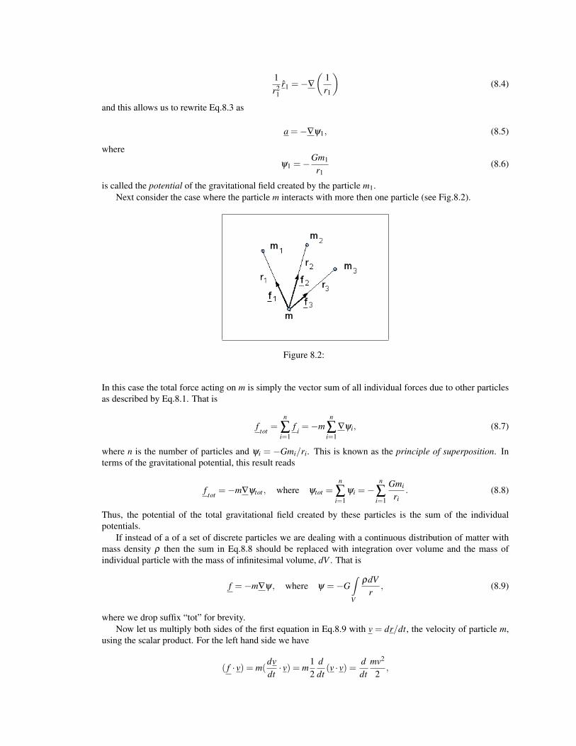
1r2
1r1 =−∇
(1r1
)(8.4)
and this allows us to rewrite Eq.8.3 as
a =−∇ψ1, (8.5)
where
ψ1 =−Gm1
r1(8.6)
is called the potential of the gravitational field created by the particle m1.Next consider the case where the particle m interacts with more then one particle (see Fig.8.2).
Figure 8.2:
In this case the total force acting on m is simply the vector sum of all individual forces due to other particlesas described by Eq.8.1. That is
ftot
=n
∑i=1
fi=−m
n
∑i=1
∇ψi, (8.7)
where n is the number of particles and ψi = −Gmi/ri. This is known as the principle of superposition. Interms of the gravitational potential, this result reads
ftot
=−m∇ψtot , where ψtot =n
∑i=1
ψi =−n
∑i=1
Gmi
ri. (8.8)
Thus, the potential of the total gravitational field created by these particles is the sum of the individualpotentials.
If instead of a of a set of discrete particles we are dealing with a continuous distribution of matter withmass density ρ then the sum in Eq.8.8 should be replaced with integration over volume and the mass ofindividual particle with the mass of infinitesimal volume, dV . That is
f =−m∇ψ, where ψ =−G∫V
ρdVr
, (8.9)
where we drop suffix “tot” for brevity.Now let us multiply both sides of the first equation in Eq.8.9 with v = dr/dt, the velocity of particle m,
using the scalar product. For the left hand side we have
( f · v) = m(dvdt· v) = m
12
ddt(v · v) = d
dtmv2
2,
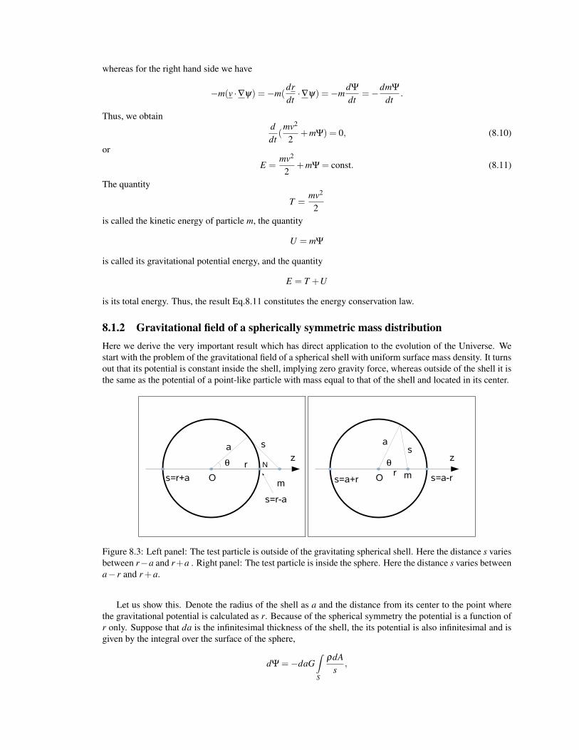
whereas for the right hand side we have
−m(v ·∇ψ) =−m(drdt·∇ψ) =−m
dΨdt
=−dmΨdt
.
Thus, we obtainddt(
mv2
2+mΨ) = 0, (8.10)
or
E =mv2
2+mΨ = const. (8.11)
The quantity
T =mv2
2is called the kinetic energy of particle m, the quantity
U = mΨ
is called its gravitational potential energy, and the quantity
E = T +U
is its total energy. Thus, the result Eq.8.11 constitutes the energy conservation law.
8.1.2 Gravitational field of a spherically symmetric mass distributionHere we derive the very important result which has direct application to the evolution of the Universe. Westart with the problem of the gravitational field of a spherical shell with uniform surface mass density. It turnsout that its potential is constant inside the shell, implying zero gravity force, whereas outside of the shell it isthe same as the potential of a point-like particle with mass equal to that of the shell and located in its center.
a
r
s
mOs=r+a
s=r-a
Nz
a
r
s
mO s=a-rs=a+r
z
Figure 8.3: Left panel: The test particle is outside of the gravitating spherical shell. Here the distance s variesbetween r−a and r+a . Right panel: The test particle is inside the sphere. Here the distance s varies betweena− r and r+a.
Let us show this. Denote the radius of the shell as a and the distance from its center to the point wherethe gravitational potential is calculated as r. Because of the spherical symmetry the potential is a function ofr only. Suppose that da is the infinitesimal thickness of the shell, the its potential is also infinitesimal and isgiven by the integral over the surface of the sphere,
dΨ =−daG∫S
ρdAs
,
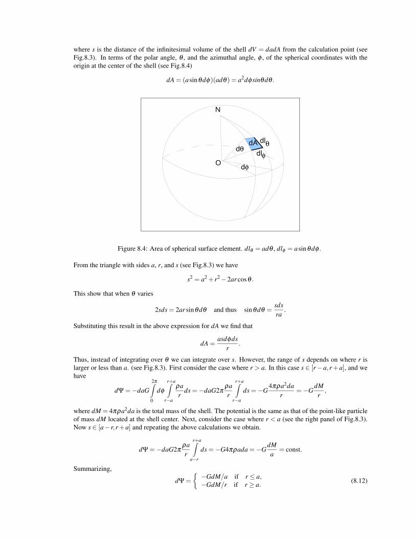
where s is the distance of the infinitesimal volume of the shell dV = dadA from the calculation point (seeFig.8.3). In terms of the polar angle, θ , and the azimuthal angle, φ , of the spherical coordinates with theorigin at the center of the shell (see Fig.8.4)
dA = (asinθdφ)(adθ) = a2dφsinθdθ .
d
ddA
O
N
dl
dl
Figure 8.4: Area of spherical surface element. dlθ = adθ , dlφ = asinθdφ .
From the triangle with sides a, r, and s (see Fig.8.3) we have
s2 = a2 + r2−2ar cosθ .
This show that when θ varies
2sds = 2ar sinθdθ and thus sinθdθ =sdsra
.
Substituting this result in the above expression for dA we find that
dA =asdφds
r.
Thus, instead of integrating over θ we can integrate over s. However, the range of s depends on where r islarger or less than a. (see Fig.8.3). First consider the case where r > a. In this case s ∈ [r−a,r+a], and wehave
dΨ =−daG2π∫0
dφ
r+a∫r−a
ρar
ds =−daG2πρar
r+a∫r−a
ds =−G4πρa2da
r=−G
dMr
,
where dM = 4πρa2da is the total mass of the shell. The potential is the same as that of the point-like particleof mass dM located at the shell center. Next, consider the case where r < a (see the right panel of Fig.8.3).Now s ∈ [a− r,r+a] and repeating the above calculations we obtain.
dΨ =−daG2πρar
r+a∫a−r
ds =−G4πρada =−GdMa
= const.
Summarizing,
dΨ =
−GdM/a if r ≤ a,−GdM/r if r ≥ a. (8.12)
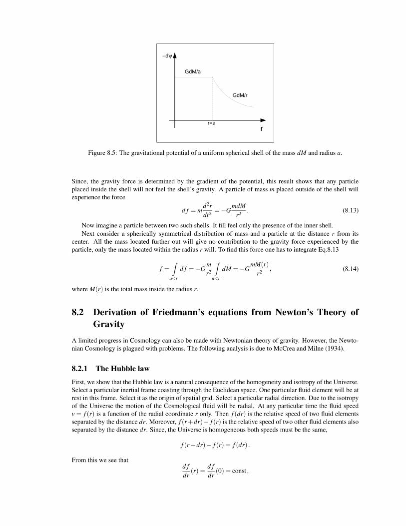
d
GdM/a
GdM/r
rr=a
Figure 8.5: The gravitational potential of a uniform spherical shell of the mass dM and radius a.
Since, the gravity force is determined by the gradient of the potential, this result shows that any particleplaced inside the shell will not feel the shell’s gravity. A particle of mass m placed outside of the shell willexperience the force
d f = md2rdt2 =−G
mdMr2 . (8.13)
Now imagine a particle between two such shells. It fill feel only the presence of the inner shell.Next consider a spherically symmetrical distribution of mass and a particle at the distance r from its
center. All the mass located further out will give no contribution to the gravity force experienced by theparticle, only the mass located within the radius r will. To find this force one has to integrate Eq.8.13
f =∫
a<r
d f =−Gmr2
∫a<r
dM =−GmM(r)
r2 , (8.14)
where M(r) is the total mass inside the radius r.
8.2 Derivation of Friedmann’s equations from Newton’s Theory ofGravity
A limited progress in Cosmology can also be made with Newtonian theory of gravity. However, the Newto-nian Cosmology is plagued with problems. The following analysis is due to McCrea and Milne (1934).
8.2.1 The Hubble law
First, we show that the Hubble law is a natural consequence of the homogeneity and isotropy of the Universe.Select a particular inertial frame coasting through the Euclidean space. One particular fluid element will be atrest in this frame. Select it as the origin of spatial grid. Select a particular radial direction. Due to the isotropyof the Universe the motion of the Cosmological fluid will be radial. At any particular time the fluid speedv = f (r) is a function of the radial coordinate r only. Then f (dr) is the relative speed of two fluid elementsseparated by the distance dr. Moreover, f (r+dr)− f (r) is the relative speed of two other fluid elements alsoseparated by the distance dr. Since, the Universe is homogeneous both speeds must be the same,
f (r+dr)− f (r) = f (dr) .
From this we see thatd fdr
(r) =d fdr
(0) = const ,
and hence f (r) is a linear function. Denoting the constant as H0 and noticing that f(0)=0, we obtain theHubble law
v = H0r. (8.15)
Notice, that this argument allows H0 to be a function of time.Integrating Eq.8.15 we find that
r = S(t)r0 , (8.16)
where
S(t) = exp(t∫
t0
H0(t)dt).
and r0 = r(t0). Thus, the distance between any two fluid elements grows in time as S(t). r0 is an example ofso-called Lagrangian coordinates of fluid elements, coordinates which do not change in time. S(t) is simplythe scaling factor which relates this coordinate with the coordinate r.
From the last equation it follows that
H0 =SS. (8.17)
8.2.2 The Friedmann equationSince the Universe is uniform its mass distribution is obviously spherically symmetric with respect to anypoint, which can be considered as a center of symmetry. So if we take a fluid element of mass δm at thedistance r from center, then it will feel only the gravity force due to the mass M = (4π/3)r3ρ inside thesphere of radius r (see Sec.8.1.2). Thus,
δmd2rdt2 =−G
δmMr2 or r =−G
Mr2 , (8.18)
where use the familiar notation r = dr/dt, r = d2r/dt2, etc. Since this particle is simply participating inthe global expansion of the cosmological fluid, the mass M remains constant even if r increases with time.1
Thus, we are dealing with a relatively simple second order ordinary differential equation (ODE). Repeatingthe calculation leading to the energy conservation law Eq.8.11 we find
(r)2
2=
GMr−C, (8.19)
where C is a constant. Let us analyze this result. Suppose that r is positive, which corresponds to the currentlyobserved expansion of the Universe. Will it stay positive all the time or at some point the expansion will turninto a contraction? The answer depends of the sign of the constant C. Indeed, at the turning point r = 0 andthus we need to see if the right hand side of Eq.8.19 can vanish. Obviously, it cannot if C < 0 – in this case theUniverse will expand forever. It will keep expanding even if C = 0, simply because GM/r > 0. If, however,C > 0, no matter by how much, there will be a turning point. Indeed, as r increases GM/r tends to zero andthe right hand side of Eq.8.19 will eventually vanish. At this point, the Universe will begin to contract. Infact, the speed corresponding to C = 0,
v =
√2GM
r, (8.20)
is known in the Newton’s theory of gravity as the escape speed. This is the minimum speed in the radialdirection a projectile must have in order to escape from the gravitational field of mass M, whose center islocated at distance r from the projectile.
We can rewrite Eq.8.19 in a somewhat more convenient form if we substitute the expression for M andmultiply both sides by 2/r2. This gives (
rr
)2
=8π
3Gρ− 2C
r2 . (8.21)
1In fact, as we shell see later, the inclusion of mass-energy associated with heat allows M to vary, so here we are cheating a bit.
Substituting into this equation the expression for r from Eq.8.16 we obtain(SS
)2
=8π
3Gρ− 2C
r20S2 .
This shows that Eq.8.21 is consistent with the uniform expansion if C ∝ r20 (only in this case we have the
same equation for the scaling factor for any r0). So we may put C = r20(A/2), where A is the same constant
for all r0, and obtain (SS
)2
=8π
3Gρ− A
S2 .
This equation already has the form similar to that of the Friedmann equation. It can take exactly the sameform after a simple rescaling. Indeed, introduce new scaling factor R(t) via
R =
cS if A = 0cS/√
A if A > 0cS/√−A if A < 0
Then the above equation becomes (RR
)2
=8π
3Gρ− kc2
R2 , (8.22)
where k is either 0, +1, or -1. This change of scaling requires to change the Lagrangian coordinate to
χ =
r0/c if A = 0(r0/c)
√A if A > 0
(r0/c)√−A if A < 0
,
so thatr = R(t)χ.
One can see that the Lagrangian coordinate χ can be interpreted as the radial coordinate at the time t0 whenR = 1.
It is easy to see that (RR
)= H0
for all three possible values of k.
8.2.3 The fluid equationThe Friedmann equation can be solved for R(t) provided we know ρ(t). Thus we need an additional equationto determine the evolution of the inertial, and hence the gravitational, mass density of the cosmological fluid.According to the first law of thermodynamics, when a fluid is expanding adiabatically
dE =−PdV (8.23)
where P is the fluid pressure, V is its volume, and E is its internal energy. In fact this is the energy conservationlaw: as the fluid expands it carries out work PdV on its surrounding, at the expense of its internal energy. Forexample, consider gas in a cylinder containing a piston with area A. The pressure force acting on the pistonis pA. When the piston moves by dx, the work done by the gas is PAdx = PdV .
Equation 8.23 can be written in terms of time derivatives as
E =−PV . (8.24)
This law can be applied to the sphere of expanding cosmological fluid. Its volume is
V =43
πr3 =43
πR3χ
3.
At this point we cheat a bit again and use the relativistic mass-energy equation:
E = Mc2 = ρc2V =43
πR3χ
3ρc2.
Substituting these expressions into Eq.8.24 we obtain
ρ =−3(
RR
)(ρ +
Pc2
), (8.25)
(recall that χ=const and hence χ = 0) which is exactly the same as Eq.3.20.
8.2.4 The acceleration equationIn order to obtain the acceleration equation we first differentiate the Friedmann equation (Eq.8.22) withrespect to time
2RR
(RR− R2
R2
)− 2kc2
R2RR=
8π
3Gρ.
Next we substitute in this equation the expression for 2kc2/R2 from the Friedmann equation and obtain
2RR
[RR− 8π
3Gρ
]=
8π
3Gρ.
Finally, we substitute the expression for ρ from the fluid equation and simplify the result by cancelling thecommon factor R/R and rearranging the terms. This gives us
RR=−4πG
3
(ρ +3
Pc2
), (8.26)
which is the acceleration equation Eq.3.19.
8.2.5 Newton’s law of gravity with cosmological constantIn order do derive the Friedmann equation with the cosmological term we need to modify the Newton’s lawof gravity (Eq.8.1) by including a term with the cosmological constant. The modified equation is
f1=−Gm1m
r21
r1 +13
Λmr1r1. (8.27)
Notice that for Λ> 0 the new term corresponds to a repulsion force. Via repeating the calculations of Sections8.1 and 8.2.2 one can derive Eq.3.21.
8.2.6 The key inconsistencies of the Newtonian CosmologyThe argument that one can choose any point in space as a center of spherical symmetry and then apply theresults obtained in Sec,8.1.2 is wrong as it leads to conflict with the assumption of homogeneous Universe.Indeed, all gravity force vectors point towards one point in space, the selected center of spherical symmetry.This makes this point very special, which in clear conflict with the assumption of homogeneous Universe.Only the everywhere vanishing gravity force is consistent with the homogeneity and isotropy of the Universe.In Newtonian cosmology, equation 8.18 makes sense only if the Universe has a center (and the Earth islocated close to it).
Second, although the theory of relativity is utilized in the derivation of the fluid equation (see Sec.8.2.3),the Newtonian cosmology is inconsistent with the speed of light being the highest possible speed. Indeed,Eq.8.15 shows that v→ ∞ when r→ ∞. (Notice that because the space of Newtonian theory is Euclidean rvaries from 0 to ∞.)


![[esoteric] Musical Theory and Ancient Cosmology.pdf](https://img.pdfslide.net/doc/110x75/55cf9936550346d0339c365c/esoteric-musical-theory-and-ancient-cosmologypdf.jpg)