Embed Size (px)
Citation preview
Cosmos DB for MongoDB Developers
Migrating to Azure Cosmos DB and Using the MongoDB API—Manish Sharma
www.allitebooks.com
Cosmos DB for MongoDB DevelopersMigrating to Azure Cosmos DB
and Using the MongoDB API
Manish Sharma
www.allitebooks.com
Cosmos DB for MongoDB Developers: Migrating to Azure Cosmos DB and Using the MongoDB API
ISBN-13 (pbk): 978-1-4842-3681-9 ISBN-13 (electronic): 978-1-4842-3682-6https://doi.org/10.1007/978-1-4842-3682-6
Library of Congress Control Number: 2018953685
Copyright © 2018 by Manish Sharma
This work is subject to copyright. All rights are reserved by the Publisher, whether the whole or part of the material is concerned, specifically the rights of translation, reprinting, reuse of illustrations, recitation, broadcasting, reproduction on microfilms or in any other physical way, and transmission or information storage and retrieval, electronic adaptation, computer software, or by similar or dissimilar methodology now known or hereafter developed.
Trademarked names, logos, and images may appear in this book. Rather than use a trademark symbol with every occurrence of a trademarked name, logo, or image, we use the names, logos, and images only in an editorial fashion and to the benefit of the trademark owner, with no intention of infringement of the trademark.
The use in this publication of trade names, trademarks, service marks, and similar terms, even if they are not identified as such, is not to be taken as an expression of opinion as to whether or not they are subject to proprietary rights.
While the advice and information in this book are believed to be true and accurate at the date of publication, neither the author nor the editors nor the publisher can accept any legal responsibility for any errors or omissions that may be made. The publisher makes no warranty, express or implied, with respect to the material contained herein.
Managing Director, Apress Media LLC: Welmoed SpahrAcquisitions Editor: Smriti SrivastavaDevelopment Editor: Matthew MoodieCoordinating Editor: Divya Modi
Cover designed by eStudioCalamar
Cover image designed by Freepik (www.freepik.com)
Distributed to the book trade worldwide by Springer Science+Business Media New York, 233 Spring Street, 6th Floor, New York, NY 10013. Phone 1-800-SPRINGER, fax (201) 348-4505, e-mail [email protected], or visit www.springeronline.com. Apress Media, LLC is a California LLC and the sole member (owner) is Springer Science+Business Media Finance Inc (SSBM Finance Inc). SSBM Finance Inc is a Delaware corporation.
For information on translations, please e-mail [email protected], or visit www.apress.com/rights-permissions.
Apress titles may be purchased in bulk for academic, corporate, or promotional use. eBook versions and licenses are also available for most titles. For more information, reference our Print and eBook Bulk Sales web page at www.apress.com/bulk-sales.
Any source code or other supplementary material referenced by the author in this book is available to readers on GitHub via the book’s product page, located at www.apress.com/9781484236819. For more detailed information, please visit www.apress.com/source-code.
Printed on acid-free paper
Manish SharmaFaridabad, Haryana, India
www.allitebooks.com

For Shweta, my sweetheart, unfailing support and my ocean of emotions
www.allitebooks.com
v
Table of Contents
Chapter 1: Why NoSQL? ������������������������������������������������������������������������1
Types of NoSQL �����������������������������������������������������������������������������������������������������2
Key-Value Pair �������������������������������������������������������������������������������������������������2
Columnar ���������������������������������������������������������������������������������������������������������3
Document ��������������������������������������������������������������������������������������������������������3
Graph ���������������������������������������������������������������������������������������������������������������4
What to Expect from NoSQL ����������������������������������������������������������������������������������6
Atomicity ��������������������������������������������������������������������������������������������������������6
Consistency �����������������������������������������������������������������������������������������������������6
Isolation �����������������������������������������������������������������������������������������������������������6
Durability ���������������������������������������������������������������������������������������������������������6
Consistency �����������������������������������������������������������������������������������������������������7
Availability �������������������������������������������������������������������������������������������������������7
Partition Tolerance �������������������������������������������������������������������������������������������7
Example 1: Availability �������������������������������������������������������������������������������������8
Example 2: Consistency �����������������������������������������������������������������������������������8
About the Author ���������������������������������������������������������������������������������xi
About the Technical Reviewer �����������������������������������������������������������xiii
Acknowledgments ������������������������������������������������������������������������������xv
Introduction ��������������������������������������������������������������������������������������xvii
www.allitebooks.com
vi
NoSQL and Cloud ��������������������������������������������������������������������������������������������������8
IaaS������������������������������������������������������������������������������������������������������������������9
PaaS ����������������������������������������������������������������������������������������������������������������9
SaaS ��������������������������������������������������������������������������������������������������������������10
Conclusion ����������������������������������������������������������������������������������������������������������10
Chapter 2: Azure Cosmos DB Overview ����������������������������������������������11
Data Model Overview ������������������������������������������������������������������������������������������12
Provisioning Azure Cosmos DB ���������������������������������������������������������������������������13
Turnkey Global Distribution ���������������������������������������������������������������������������������25
Latency ����������������������������������������������������������������������������������������������������������29
Consistency ���������������������������������������������������������������������������������������������������30
Throughput ����������������������������������������������������������������������������������������������������30
Availability �����������������������������������������������������������������������������������������������������30
Reliability �������������������������������������������������������������������������������������������������������31
Protocol Support and Multimodal API �����������������������������������������������������������������32
Table Storage API �������������������������������������������������������������������������������������������32
SQL (DocumentDB) API ����������������������������������������������������������������������������������34
MongoDB API ������������������������������������������������������������������������������������������������38
Graph API �������������������������������������������������������������������������������������������������������41
Cassandra API ������������������������������������������������������������������������������������������������48
Elastic Scale ��������������������������������������������������������������������������������������������������������49
Throughput ����������������������������������������������������������������������������������������������������49
Storage ����������������������������������������������������������������������������������������������������������49
Consistency ���������������������������������������������������������������������������������������������������������50
Strong ������������������������������������������������������������������������������������������������������������50
Performance ��������������������������������������������������������������������������������������������������54
Table of ConTenTsTable of ConTenTs
vii
Service Level Agreement (SLA) ���������������������������������������������������������������������������55
Availability SLA ����������������������������������������������������������������������������������������������55
Throughput SLA ���������������������������������������������������������������������������������������������56
Consistency SLA ��������������������������������������������������������������������������������������������58
Latency SLA ���������������������������������������������������������������������������������������������������59
Conclusion ����������������������������������������������������������������������������������������������������������59
Chapter 3: Azure Cosmos DB Geo-Replication ������������������������������������61
Database Availability (DA) �����������������������������������������������������������������������������������62
MongoDB Replication ������������������������������������������������������������������������������������������62
Data-Bearing Nodes ��������������������������������������������������������������������������������������62
Arbiter Nodes �������������������������������������������������������������������������������������������������64
Azure Cosmos DB Replication �����������������������������������������������������������������������������67
Auto-Shifting Geo APIs ����������������������������������������������������������������������������������������72
Consistency and Global Distribution �������������������������������������������������������������������78
Conclusion ����������������������������������������������������������������������������������������������������������79
Chapter 4: Indexing ����������������������������������������������������������������������������81
Indexing in MongoDB ������������������������������������������������������������������������������������������81
Single Field Index ������������������������������������������������������������������������������������������82
Compound Index ��������������������������������������������������������������������������������������������87
Multikey Index �����������������������������������������������������������������������������������������������88
Geospatial Index ��������������������������������������������������������������������������������������������88
Text Index ������������������������������������������������������������������������������������������������������91
Hashed Index �������������������������������������������������������������������������������������������������93
Indexing in Azure Cosmos DB �����������������������������������������������������������������������������93
TTL Indexes ���������������������������������������������������������������������������������������������������95
Array Indexes �������������������������������������������������������������������������������������������������96
Table of ConTenTsTable of ConTenTs
viii
Sparse Indexes ����������������������������������������������������������������������������������������������97
Unique Indexes ����������������������������������������������������������������������������������������������97
Custom Indexing �������������������������������������������������������������������������������������������������98
Indexing Modes ���������������������������������������������������������������������������������������������99
Indexing Paths ���������������������������������������������������������������������������������������������104
Index Kinds ��������������������������������������������������������������������������������������������������105
Index Precision ��������������������������������������������������������������������������������������������108
Data Types ���������������������������������������������������������������������������������������������������108
Conclusion ��������������������������������������������������������������������������������������������������������108
Chapter 5: Partitioning ���������������������������������������������������������������������109
Sharding ������������������������������������������������������������������������������������������������������������109
Partitioning in Azure Cosmos DB�����������������������������������������������������������������������113
Optimizations ����������������������������������������������������������������������������������������������������122
Selecting a Partition Key �����������������������������������������������������������������������������������126
Use Case ������������������������������������������������������������������������������������������������������126
Evaluate Every Field to Be a Potential Partition Key ������������������������������������127
Selection of the Partition Key ����������������������������������������������������������������������128
Conclusion ��������������������������������������������������������������������������������������������������������135
Chapter 6: Consistency ���������������������������������������������������������������������137
Consistency in Distributed Databases���������������������������������������������������������������137
Consistency in MongoDB ����������������������������������������������������������������������������������140
Consistency in Azure Cosmos DB ����������������������������������������������������������������������142
Consistent Reads/Writes �����������������������������������������������������������������������������142
High Throughput ������������������������������������������������������������������������������������������148
Conclusion ��������������������������������������������������������������������������������������������������������153
Table of ConTenTsTable of ConTenTs
ix
Chapter 7: Sizing ������������������������������������������������������������������������������155
Request Units (RUs) ������������������������������������������������������������������������������������������155
Allocation of RUs �����������������������������������������������������������������������������������������������156
Calculating RUs �������������������������������������������������������������������������������������������������159
Optimizing RU Consumption �����������������������������������������������������������������������������164
Document Size and Complexity ������������������������������������������������������������������164
Data Consistency ����������������������������������������������������������������������������������������168
Indexing ������������������������������������������������������������������������������������������������������171
Query Patterns ��������������������������������������������������������������������������������������������176
Conclusion ��������������������������������������������������������������������������������������������������������177
Chapter 8: Migrating to Azure Cosmos DB–MongoDB API ����������������179
Migration Strategies �����������������������������������������������������������������������������������������179
mongoexport and mongoimport ������������������������������������������������������������������180
For Windows mongodump/mongorestore ���������������������������������������������������181
Application Switch ��������������������������������������������������������������������������������������������184
Optimization ������������������������������������������������������������������������������������������������������186
Conclusion ��������������������������������������������������������������������������������������������������������188
Chapter 9: Azure Cosmos DB–MongoDB API Advanced Services �����191
Aggregation Pipeline �����������������������������������������������������������������������������������������191
Spark Connector �����������������������������������������������������������������������������������������������196
Conclusion ��������������������������������������������������������������������������������������������������������204
Index �������������������������������������������������������������������������������������������������205
Table of ConTenTsTable of ConTenTs
xi
About the Author
Manish Sharma is a senior technology
evangelist at Microsoft. He has 14 years
of experience at various organizations
and is primarily involved in technological
enhancements. He is a certified Azure
solutions architect, AWS-certified solutions
architect, cloud data architect, .NET solutions
developer, and PMP-certified project manager.
He is a regular speaker at various technical
conferences organized by Microsoft (Future
Decoded, Azure, and specialized webinars)
and its community (GIDS, Docker, etc.) on
client-server, cloud, and data technologies.
xiii
About the Technical Reviewer
Andre Essing advises customers on all
topics related to the Microsoft data platform,
in his capacity as a technology solutions
professional. Since version 7.0, Andre has
acquired experience with the SQL Server
product family, for which he has focused on
infrastructure topics, mission-critical systems,
and security. Today, Andre concentrates
on working with data in the cloud, such as
modern data warehouse architectures, artificial intelligence, and new
scalable database systems, such as Azure Cosmos DB.
In addition to his work at Microsoft, Andre is engaged in the
community as a leader of the Bavaria, Germany, chapter of the
Professional Association for SQL Server (PASS). You can find him as a
speaker at various user groups and international conferences.
xv
Acknowledgments
I would like to express appreciation to my special team: Govind Kanshi,
who helped me along the entire journey, and Sandeep Alur, through whose
inspiration I was able to write this book.
xvii
Introduction
It was a wonderful experience when I first encountered Azure Cosmos
DB–MongoDB API, as this is a new entrant to the technological world with
a promising future. While writing this book, I was able to experience a few
pre-released features, now available, which I have referred to in the text.
During my sessions, I always suggest that architects do their due
diligence while architecting solutions, as any technology can make or
break a system drastically.
This book is specifically focused on making sure that, coming from a
MongoDB background, you will avoid roadblocks and will make informed
decisions. You have made the right choice by starting to learn Azure
Cosmos DB–MongoDB API, which will take your existing skills to the next
level and give you an edge in the cloud era.
MongoDB has been used in the industry for quite a while and has
already hit the roof on-premises worldwide. With the inception of cloud
native databases such as Azure Cosmos DB, any NoSQL must now offer
unlimited scaling, be always on, and have multiple data centers. This book
will guide you in identifying the whys and hows that you can employ in
your applications and help in achieving extraordinary success.
The structure of this book provides an inside look into each aspect of
Azure Cosmos DB. If you are new to NoSQL, I will suggest you start from
Chapter 1; otherwise, jump directly to Chapter 2. Chapters 3 to 6 provide
specialized coverage, respectively, of the topics introduced in Chapter 1.
Chapter 7 is important, as before adopting to modern technology, we
must discuss how much it costs. I recommend that you perform some
experiments, based on your specific situation, before arriving at actual
xviii
costs. Chapter 8 covers aspects related to data migration. Chapter 9
provides detailed information about one of the most loved MongoDB
features, the aggregation pipeline.
Feeling Excited? Cool.
Now it’s time to turn the page and start your journey.
InTroduCTIonInTroduCTIon
1© Manish Sharma 2018 M. Sharma, Cosmos DB for MongoDB Developers, https://doi.org/10.1007/978-1-4842-3682-6_1
CHAPTER 1
Why NoSQL?Since schooling most of us are taught to structure information, such
that it can be represented in tabular form. But not all information can
follow that structure, hence the existence of NULL values. The NULL value
represents cells without information. To avoid NULLs, we must split one
table into multiples, thus introducing the concept of normalization. In
normalization, we split the tables, based on the level of normalization
we select. These levels are 1NF (first normal form), 2NF, 3NF, BCNF
(Boyce–Codd normal form, or 3.5NF), 4NF, and 5NF, to name just a few.
Every level dictates the split, and, most commonly, people use 3NF,
which is largely free of insert, update, and delete anomalies.
To achieve normalization, one must split information into multiple
tables and then, while retrieving, join all the tables to make sense of the
split information. This concept poses few problems, and it is still perfect
for online transaction processing (OLTP).
Working on a system that handles data populated from multiple data
streams and adheres to one defined structure is extremely difficult to
implement and maintain. The volume of data is often humongous and
mostly unpredictable. In such cases, splitting data into multiple pieces
while inserting and joining the tables during data retrieval will add
excessive latency.
We can solve this problem by inserting the data in its natural form.
As there is no or minimal transformation required, the latency during
inserting, updating, deleting, and retrieving will be drastically reduced.

2
With this, scaling up and scaling out will be quick and manageable.
Given the flexibility of this solution, it is the most appropriate one for the
problem defined. The solution is NoSQL, also referred to as not only, or
non-relational, SQL.
One can further prioritize performance over consistency, which is
possible with a NoSQL solution and defined by the CAP (consistency,
availability, and partition tolerance) theorem. In this chapter, I will
discuss NoSQL, its diverse types, its comparison with relational database
management systems (RDBMS), and its future applications.
Types of NoSQLIn NoSQL, data can be represented in multiple forms. Many forms of
NoSQL exist, and the most commonly used ones are key-value, columnar,
document, and graph. In this section, I will summarize the forms most
commonly used.
Key-Value PairThis is the simplest data structure form but offers excellent performance.
All the data is referred only through keys, making retrieval very
straightforward. The most popular database in this category is Redis
Cache. An example is shown in Table 1-1.
Table 1-1. Key-Value Representation
Key Value
C1 XXX XXXX XXXX
C2 123456789
C3 10/01/2005
C4 ZZZ ZZZZ ZZZZ
Chapter 1 Why NoSQL?
3
The keys are in the ordered list, and a HashMap is used to locate the
keys effectively.
ColumnarThis type of database stores the data as columns instead of rows (as
RDBMS do) and are optimized for querying large data sets. This type of
database is generally known as a wide column store. Some of the most
popular databases in this category include Cassandra, Apache Hadoop’s
HBase, etc.
Unlike key-value pair databases, columnar databases can store
millions of attributes associated with the key forming a table, but stored
as columns. However, being a NoSQL database, it will not have any fixed
name or number of columns, which makes it a true schema-free database.
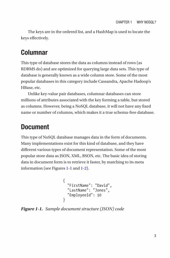
DocumentThis type of NoSQL database manages data in the form of documents.
Many implementations exist for this kind of database, and they have
different various types of document representation. Some of the most
popular store data as JSON, XML, BSON, etc. The basic idea of storing
data in document form is to retrieve it faster, by matching to its meta
information (see Figures 1-1 and 1-2).
{ "FirstName": "David", "LastName": "Jones", "EmployeeId": 10 }
Figure 1-1. Sample document structure (JSON) code
Chapter 1 Why NoSQL?
4
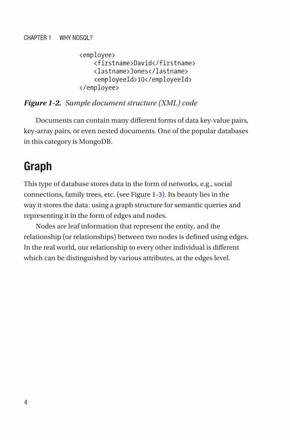
Documents can contain many different forms of data key-value pairs,
key-array pairs, or even nested documents. One of the popular databases
in this category is MongoDB.
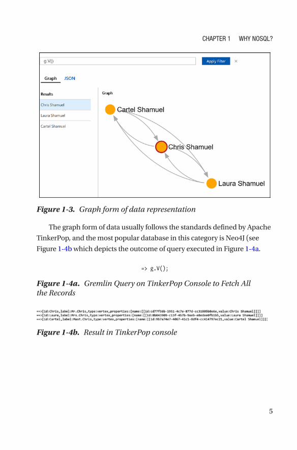
GraphThis type of database stores data in the form of networks, e.g., social
connections, family trees, etc. (see Figure 1-3). Its beauty lies in the
way it stores the data: using a graph structure for semantic queries and
representing it in the form of edges and nodes.
Nodes are leaf information that represent the entity, and the
relationship (or relationships) between two nodes is defined using edges.
In the real world, our relationship to every other individual is different
which can be distinguished by various attributes, at the edges level.
<employee> <firstname>David</firstname> <lastname>Jones</lastname> <employeeId>10</employeeId> </employee>
Figure 1-2. Sample document structure (XML) code
Chapter 1 Why NoSQL?
5
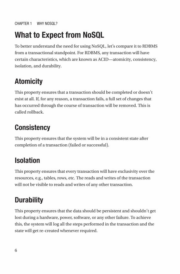
The graph form of data usually follows the standards defined by Apache
TinkerPop, and the most popular database in this category is Neo4J (see
Figure 1-4b which depicts the outcome of query executed in Figure 1-4a.
Figure 1-3. Graph form of data representation
Figure 1-4a. Gremlin Query on TinkerPop Console to Fetch All the Records
Figure 1-4b. Result in TinkerPop console
Chapter 1 Why NoSQL?
6
What to Expect from NoSQLTo better understand the need for using NoSQL, let’s compare it to RDBMS
from a transactional standpoint. For RDBMS, any transaction will have
certain characteristics, which are known as ACID—atomicity, consistency,
isolation, and durability.
Atomicity This property ensures that a transaction should be completed or doesn’t
exist at all. If, for any reason, a transaction fails, a full set of changes that
has occurred through the course of transaction will be removed. This is
called rollback.
ConsistencyThis property ensures that the system will be in a consistent state after
completion of a transaction (failed or successful).
IsolationThis property ensures that every transaction will have exclusivity over the
resources, e.g., tables, rows, etc. The reads and writes of the transaction
will not be visible to reads and writes of any other transaction.
DurabilityThis property ensures that the data should be persistent and shouldn’t get
lost during a hardware, power, software, or any other failure. To achieve
this, the system will log all the steps performed in the transaction and the
state will get re-created whenever required.
Chapter 1 Why NoSQL?
7
By contrast, NoSQL relies on the concept of the CAP theorem, as
follows.
ConsistencyThis ensures that the read performed by any transaction has the latest
information/data for all the nodes. It is a bit different from the consistency
defined in ACID, as ACID’s consistency states that all the data changes
should provide a consistent data view for database connections.
AvailabilityEvery time data is requested, a response is given without a guarantee of the
latest data. This is critical for systems that require high performance and
tolerate eventuality of data.
Partition ToleranceThis property will ensure that network failure between nodes will not
impact the system failure or performance. It will help ensuring the
availability of the system and consistent performance.
Most of the time, in a durable distributed system, network durability
will be built in, which helps make all the nodes (partitions) available all the
time. This means we are left with two choices, consistency or availability.
When we choose availability, the system will always process the query and
return the latest data, even if it can’t guarantee the concurrency of the data.
Another theorem, PACELC, is an extension of CAP and states that
if a system is running normally in the absence of partitions, one must
choose between latency and consistency. If the system is designed for
high availability, one must replicate it, then a trade-off occurs between
consistency and latency.
Chapter 1 Why NoSQL?
8
Architects must, therefore, choose the right balance between
availability, consistency, and latency while defining the partition tolerance.
Following are a few examples.
Example 1: AvailabilityConsider, for example, a device installed on an elevator for the purpose of
monitoring that elevator. The device posts messages to the main server to
provide a status report. If something goes wrong, it will alert the relevant
personnel to perform an emergency response. Losing such a message
will jeopardize the entire emergency response system, thus selecting
availability over consistency in this case will make the most sense.
Example 2: ConsistencyConsider a reward catalog system that keeps track of allocation and
redemption of reward points. During redemption, the system must take
care of rewards accumulated at point-in-time, and the transaction should
be consistent. Otherwise, one can redeem rewards multiple times. In this
case, selection of consistency is most critical.
NoSQL and CloudNoSQL is designed to do scale out and can span thousands of computer
nodes. It has been used for quite a while and is gaining popularity because
of its unmatchable performance. However, there is no such thing as a
universal database. Hence, we should pick the best technology for the
given use case. By design, NoSQL doesn’t have rigid boundaries, unlike
other traditional systems, but it can easily hit the roof in on-premise
situations.
Chapter 1 Why NoSQL?
9
Today, industry’s needs are growing, and the focus is shifting from
capital expenditure (Capex) to operating expenses (Opex), which means
no one really wants to pay up front. This makes cloud an obvious choice
for an architect, but even in cloud, services are divided into three main
categories: infrastructure as a service (IaaS), platform as a service (PaaS),
and software as a service (SaaS). Let us look at these terms more closely.
IaaSThis is the simplest and most straightforward way to get started in the
cloud and is favored in lift-and-shift scenarios. In such scenarios, a cloud
service provider is responsible for everything up to virtualization, e.g.,
power, real estate, cooling, hardware, virtualization, etc. The onus for
everything else is on users. They must take care of the operating system,
application server, applications, etc. Example of such services include
the general-purpose virtual machine for Windows/Linux, the specialized
virtual machine for SQL Server, SharePoint, etc.
PaaSThis is best suited to application’s developers who wish to focus only on
the application and offload everything else to a cloud service provider.
PaaS will help to gain maximum scalability and performance without the
worry over the availability of end points. In this case, the cloud service
provider protects the developer up to the platform level, meaning the
base platform, e.g., the application server, database server, etc. Examples
of these services are database as a service and cache as a service, among
others.
Chapter 1 Why NoSQL?
10
SaaSIn this scenario, even the responsibility of software lies with the cloud
service provider. Everything will be offloaded to the cloud service provider,
but developers can still upload his or her customizations or integrate them
through APIs. Examples of these services include Office 365, Dynamics
365, etc.
All the previously mentioned services have their own advantages and
disadvantages. However, there is absolutely no need to stick with one type
of service. Instead, one can choose a combination of them for different
purposes. An example could be that the main application is deployed
onto the SaaS, which is integrated with Office 365. The application’s legacy
components could be deployed onto a virtual machine (IaaS), and the
database deployed onto a database as a service PaaS.
ConclusionPaaS, is the developer friendly option which is the best for application’s
developers as it will give them freedom from infrastructure management
headaches which includes availability of the database service, database
service support, management of storage, monitoring tools, etc.
I will discuss industry’s most widely and quickly adopted NoSQL
database, which is discussed as a PaaS in subsequent chapters.
Chapter 1 Why NoSQL?
11© Manish Sharma 2018 M. Sharma, Cosmos DB for MongoDB Developers, https://doi.org/10.1007/978-1-4842-3682-6_2
CHAPTER 2
Azure Cosmos DB OverviewNoSQL was conceived to address issues related to scalability, durability,
and performance. However, even highly performant systems are limited by
the computing capacity available from an on-premise machine or a virtual
machine in the cloud. In the cloud, having a massive compute-capacity
PaaS is the most desirable option, as, in this case, one needn’t worry about
scalability, performance, and availability. All of these will be provided by
the cloud service provider.
Cosmos DB is one of many PaaS services in Azure, Azure is the
name of Microsoft's public cloud offering. It was designed to consider six
key aspects: global distribution, elastic scale, throughput, well-defined
consistency models, availability, guaranteed low latency and performance,
and easy migration.
Let’s look at each aspect in detail.
12
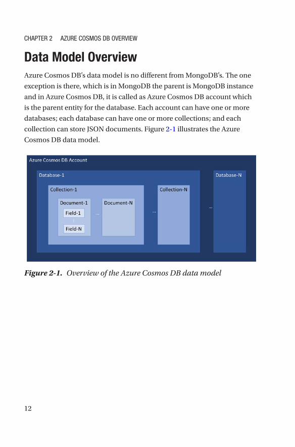
Data Model OverviewAzure Cosmos DB’s data model is no different from MongoDB’s. The one
exception is there, which is in MongoDB the parent is MongoDB instance
and in Azure Cosmos DB, it is called as Azure Cosmos DB account which
is the parent entity for the database. Each account can have one or more
databases; each database can have one or more collections; and each
collection can store JSON documents. Figure 2- 1 illustrates the Azure
Cosmos DB data model.
Figure 2-1. Overview of the Azure Cosmos DB data model
Chapter 2 azure Cosmos DB overview
13
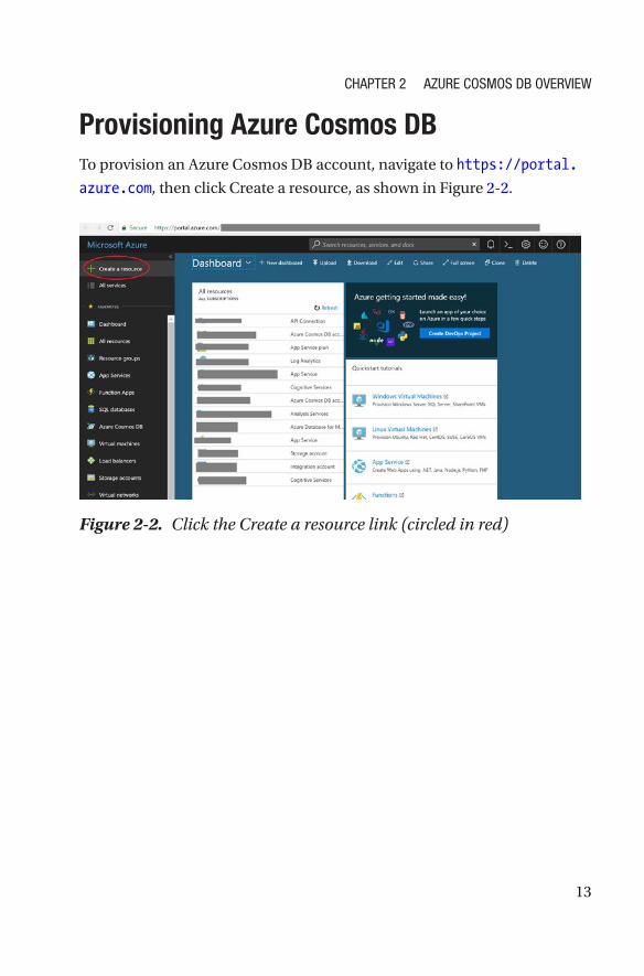
Provisioning Azure Cosmos DBTo provision an Azure Cosmos DB account, navigate to https://portal.
azure.com, then click Create a resource, as shown in Figure 2-2.
Figure 2-2. Click the Create a resource link (circled in red)
Chapter 2 azure Cosmos DB overview
14
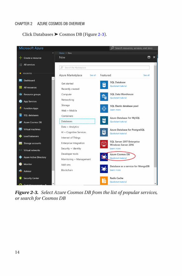
Click Databases ➤ Cosmos DB (Figure 2-3).
Figure 2-3. Select Azure Cosmos DB from the list of popular services, or search for Cosmos DB
Chapter 2 azure Cosmos DB overview
15
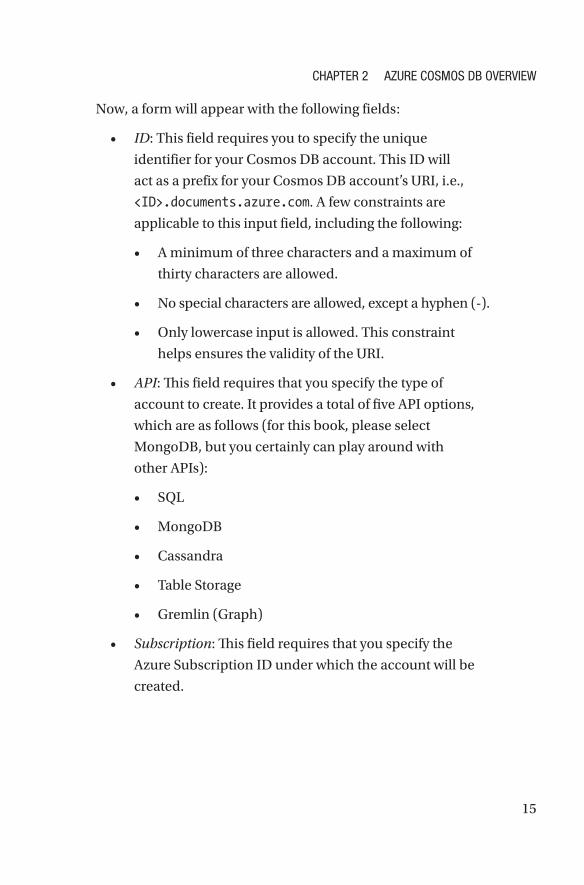
Now, a form will appear with the following fields:
• ID: This field requires you to specify the unique
identifier for your Cosmos DB account. This ID will
act as a prefix for your Cosmos DB account’s URI, i.e.,
<ID>.documents.azure.com. A few constraints are
applicable to this input field, including the following:
• A minimum of three characters and a maximum of
thirty characters are allowed.
• No special characters are allowed, except a hyphen (-).
• Only lowercase input is allowed. This constraint
helps ensures the validity of the URI.
• API: This field requires that you specify the type of
account to create. It provides a total of five API options,
which are as follows (for this book, please select
MongoDB, but you certainly can play around with
other APIs):
• SQL
• MongoDB
• Cassandra
• Table Storage
• Gremlin (Graph)
• Subscription: This field requires that you specify the
Azure Subscription ID under which the account will be
created.
Chapter 2 azure Cosmos DB overview
16
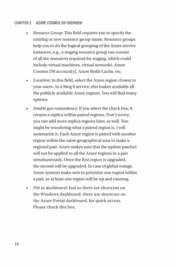
• Resource Group: This field requires you to specify the
existing or new resource group name. Resource groups
help you to do the logical grouping of the Azure service
instances, e.g., a staging resource group can consist
of all the resources required for staging, which could
include virtual machines, virtual networks, Azure
Cosmos DB account(s), Azure Redis Cache, etc.
• Location: In this field, select the Azure region closest to
your users. As a Ring 0 service, this makes available all
the publicly available Azure regions. You will find many
options.
• Enable geo-redundancy: If you select the check box, it
creates a replica within paired regions. Don’t worry;
you can add more replica regions later, as well. You
might be wondering what a paired region is. I will
summarize it. Each Azure region is paired with another
region within the same geographical area to make a
regional pair. Azure makes sure that the update patches
will not be applied to all the Azure regions in a pair
simultaneously. Once the first region is upgraded,
the second will be upgraded. In case of global outage,
Azure systems make sure to prioritize one region within
a pair, so at least one region will be up and running.
• Pin to dashboard: Just as there are shortcuts on
the Windows dashboard, there are shortcuts on
the Azure Portal dashboard, for quick access.
Please check this box.
Chapter 2 azure Cosmos DB overview
17
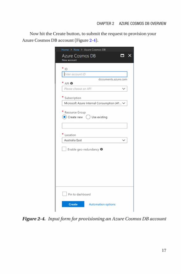
Now hit the Create button, to submit the request to provision your
Azure Cosmos DB account (Figure 2-4).
Figure 2-4. Input form for provisioning an Azure Cosmos DB account
Chapter 2 azure Cosmos DB overview
18
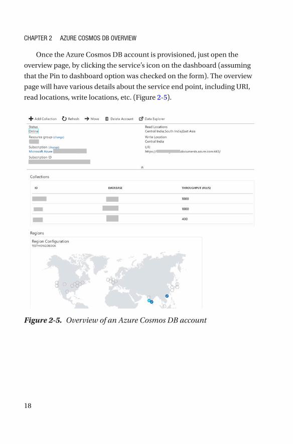
Once the Azure Cosmos DB account is provisioned, just open the
overview page, by clicking the service’s icon on the dashboard (assuming
that the Pin to dashboard option was checked on the form). The overview
page will have various details about the service end point, including URI,
read locations, write locations, etc. (Figure 2-5).
Figure 2-5. Overview of an Azure Cosmos DB account
Chapter 2 azure Cosmos DB overview
19
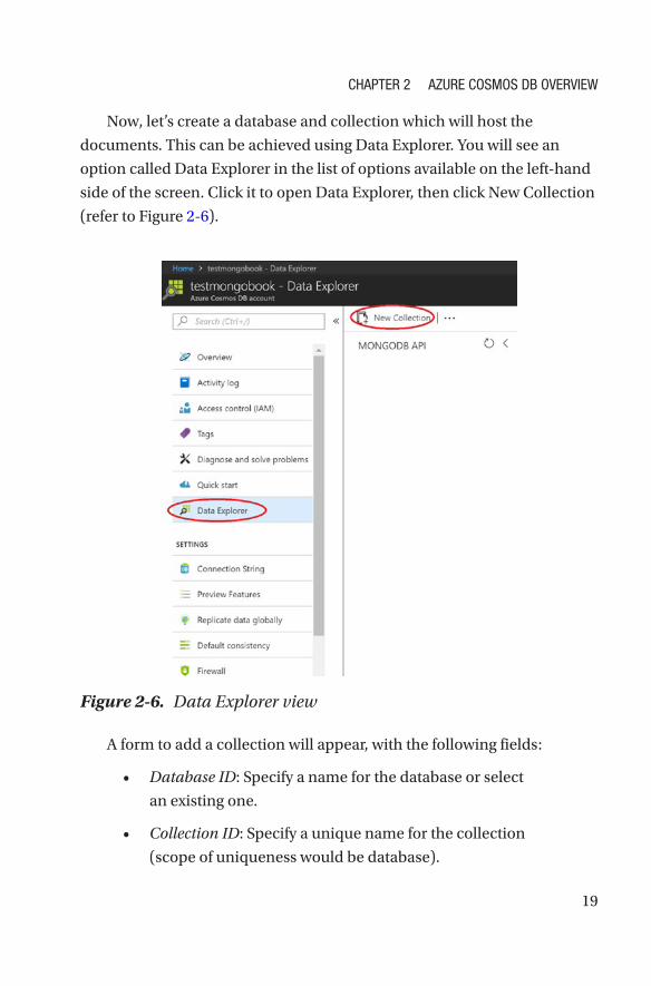
Now, let’s create a database and collection which will host the
documents. This can be achieved using Data Explorer. You will see an
option called Data Explorer in the list of options available on the left-hand
side of the screen. Click it to open Data Explorer, then click New Collection
(refer to Figure 2-6).
Figure 2-6. Data Explorer view
A form to add a collection will appear, with the following fields:
• Database ID: Specify a name for the database or select
an existing one.
• Collection ID: Specify a unique name for the collection
(scope of uniqueness would be database).
Chapter 2 azure Cosmos DB overview
20
• Storage capacity: Two options are available: Fixed
and Unlimited. With a fixed storage capacity, the size
of a collection cannot exceed 10GB. This option is
recommended if you have lean collections and would
like to pay less. Typically, this means one partition
(refer to MongoDB shard), and the maximum amount
of throughput, which is to be specified in terms of
request units (see Chapter 7 for additional information
on request units[RUs]), will also be limited in this case
(refer to the following field). To understand partitioning
in detail, see Chapter 5. The second storage capacity
option is Unlimited, whereby storage can be scaled as
required and have a wider range for request units. This
is because, multiple partitions are created behind the
scenes, to cater to your scaling requirements.
• Shard key: If the Unlimited storage option is selected, this
field will become visible (see Figure 2-7). For unlimited
storage, Azure Cosmos DB performs horizontal scaling,
which means it will have multiple partitions (shards
in MongoDB) behind the scenes. Here, Azure Cosmos
DB expects a partition key, which should be in all the
records and shouldn’t have \ & * as part of the key. The
shard key should be the field name, e.g., that of a city or a
customer address (for a nested document), etc.
• Throughput: This field is to specify initial allocation of
RUs, which are a combination of compute + memory
+ IOPS. If you have selected the Fixed storage option,
the range is from 400 to 10,000 RUs, which can’t be
extended. With the Unlimited storage option, the range
is from 1000 RUs to 100,000 RUs, which can be further
expanded by raising an Azure support call.
Chapter 2 azure Cosmos DB overview
21
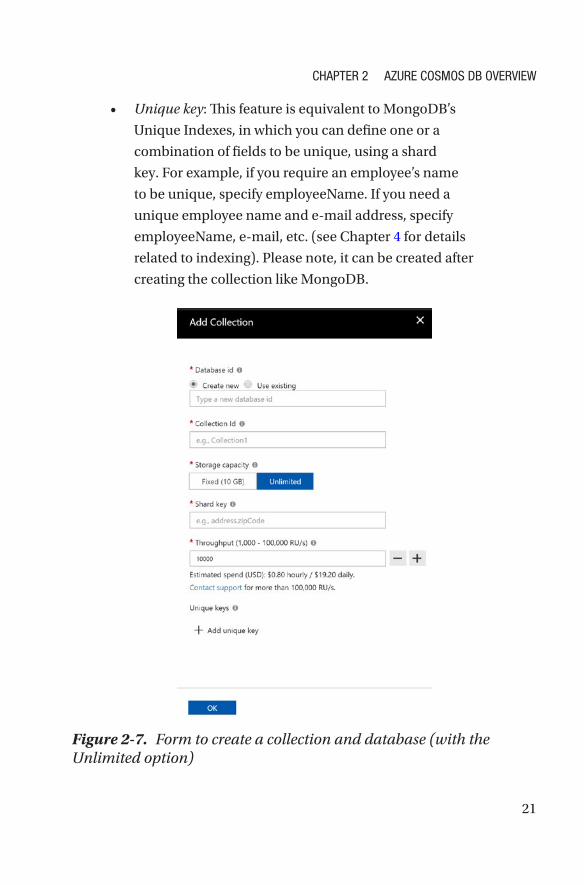
• Unique key: This feature is equivalent to MongoDB’s
Unique Indexes, in which you can define one or a
combination of fields to be unique, using a shard
key. For example, if you require an employee’s name
to be unique, specify employeeName. If you need a
unique employee name and e-mail address, specify
employeeName, e-mail, etc. (see Chapter 4 for details
related to indexing). Please note, it can be created after
creating the collection like MongoDB.
Figure 2-7. Form to create a collection and database (with the Unlimited option)
Chapter 2 azure Cosmos DB overview
22
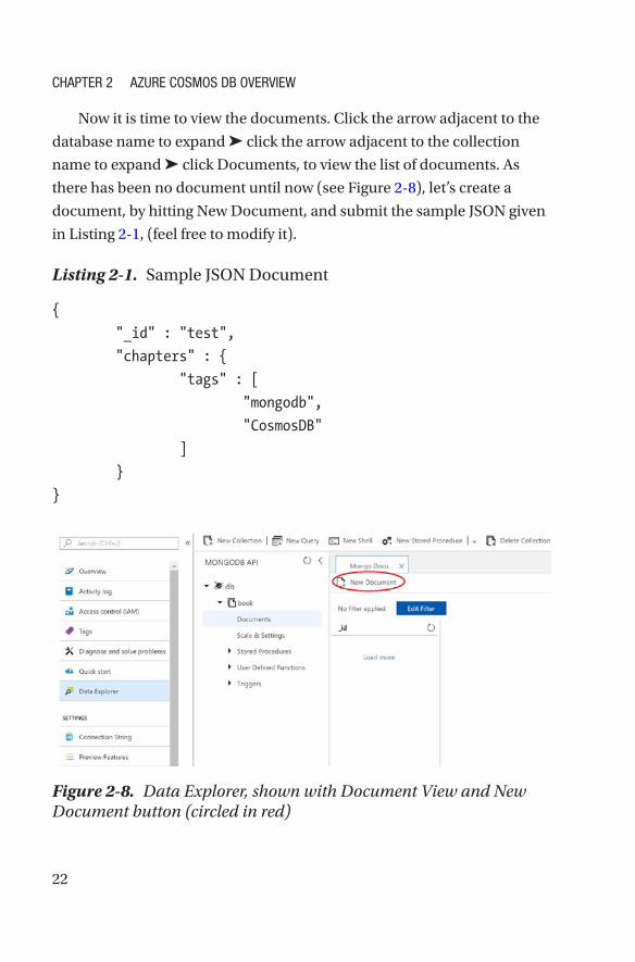
Now it is time to view the documents. Click the arrow adjacent to the
database name to expand ➤ click the arrow adjacent to the collection
name to expand ➤ click Documents, to view the list of documents. As
there has been no document until now (see Figure 2-8), let’s create a
document, by hitting New Document, and submit the sample JSON given
in Listing 2-1, (feel free to modify it).
Listing 2-1. Sample JSON Document
{
"_id" : "test",
"chapters" : {
"tags" : [
"mongodb",
"CosmosDB"
]
}
}
Figure 2-8. Data Explorer, shown with Document View and New Document button (circled in red)
Chapter 2 azure Cosmos DB overview
23
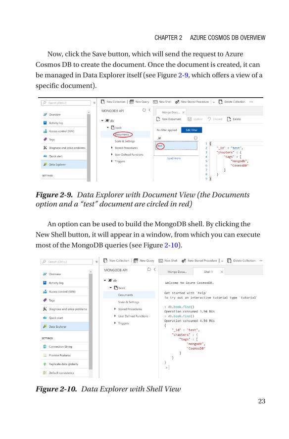
Now, click the Save button, which will send the request to Azure
Cosmos DB to create the document. Once the document is created, it can
be managed in Data Explorer itself (see Figure 2-9, which offers a view of a
specific document).
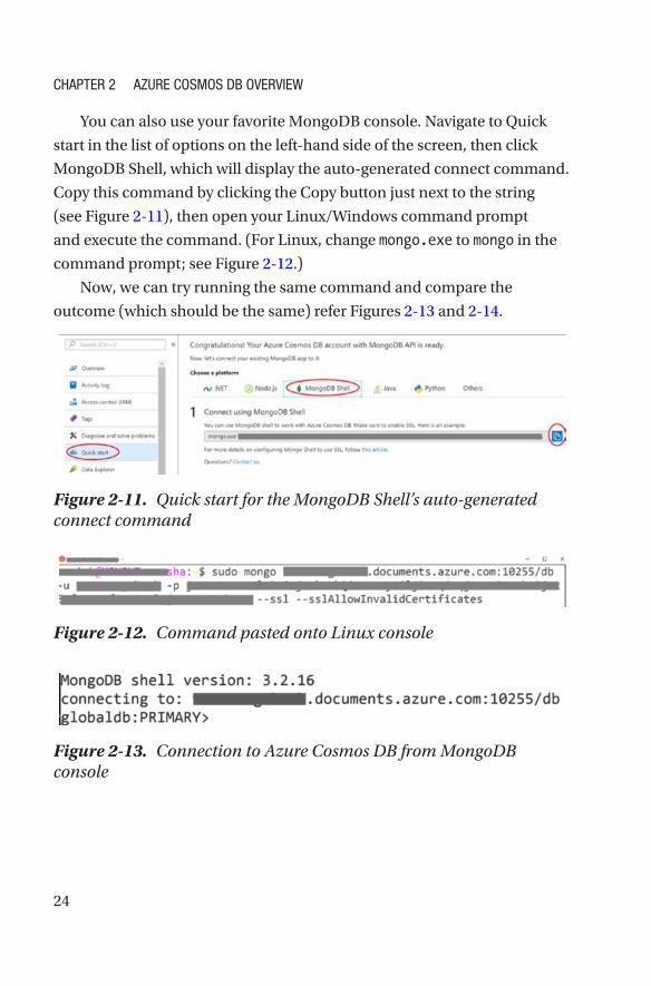
An option can be used to build the MongoDB shell. By clicking the
New Shell button, it will appear in a window, from which you can execute
most of the MongoDB queries (see Figure 2-10).
Figure 2-9. Data Explorer with Document View (the Documents option and a “test” document are circled in red)
Figure 2-10. Data Explorer with Shell View
Chapter 2 azure Cosmos DB overview
24
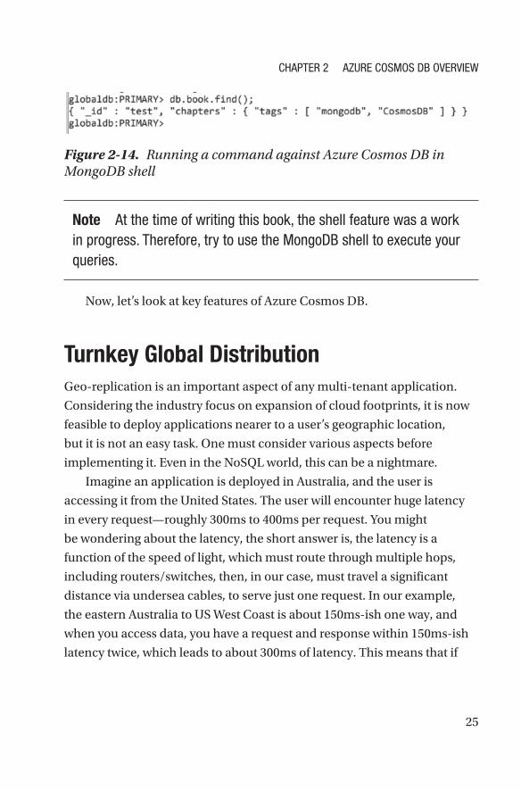
You can also use your favorite MongoDB console. Navigate to Quick
start in the list of options on the left-hand side of the screen, then click
MongoDB Shell, which will display the auto-generated connect command.
Copy this command by clicking the Copy button just next to the string
(see Figure 2-11), then open your Linux/Windows command prompt
and execute the command. (For Linux, change mongo.exe to mongo in the
command prompt; see Figure 2-12.)
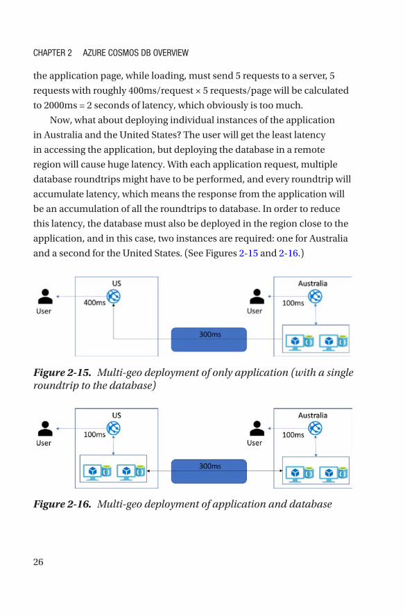
Now, we can try running the same command and compare the
outcome (which should be the same) refer Figures 2-13 and 2-14.
Figure 2-11. Quick start for the MongoDB Shell’s auto-generated connect command
Figure 2-12. Command pasted onto Linux console
Figure 2-13. Connection to Azure Cosmos DB from MongoDB console
Chapter 2 azure Cosmos DB overview
25
Note at the time of writing this book, the shell feature was a work in progress. therefore, try to use the mongoDB shell to execute your queries.
Now, let’s look at key features of Azure Cosmos DB.
Turnkey Global DistributionGeo-replication is an important aspect of any multi-tenant application.
Considering the industry focus on expansion of cloud footprints, it is now
feasible to deploy applications nearer to a user’s geographic location,
but it is not an easy task. One must consider various aspects before
implementing it. Even in the NoSQL world, this can be a nightmare.
Imagine an application is deployed in Australia, and the user is
accessing it from the United States. The user will encounter huge latency
in every request—roughly 300ms to 400ms per request. You might
be wondering about the latency, the short answer is, the latency is a
function of the speed of light, which must route through multiple hops,
including routers/switches, then, in our case, must travel a significant
distance via undersea cables, to serve just one request. In our example,
the eastern Australia to US West Coast is about 150ms-ish one way, and
when you access data, you have a request and response within 150ms-ish
latency twice, which leads to about 300ms of latency. This means that if
Figure 2-14. Running a command against Azure Cosmos DB in MongoDB shell
Chapter 2 azure Cosmos DB overview
26
the application page, while loading, must send 5 requests to a server, 5
requests with roughly 400ms/request × 5 requests/page will be calculated
to 2000ms = 2 seconds of latency, which obviously is too much.
Now, what about deploying individual instances of the application
in Australia and the United States? The user will get the least latency
in accessing the application, but deploying the database in a remote
region will cause huge latency. With each application request, multiple
database roundtrips might have to be performed, and every roundtrip will
accumulate latency, which means the response from the application will
be an accumulation of all the roundtrips to database. In order to reduce
this latency, the database must also be deployed in the region close to the
application, and in this case, two instances are required: one for Australia
and a second for the United States. (See Figures 2-15 and 2-16.)
Figure 2-15. Multi-geo deployment of only application (with a single roundtrip to the database)
Figure 2-16. Multi-geo deployment of application and database
Chapter 2 azure Cosmos DB overview
27
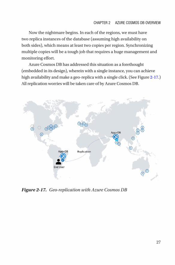
Now the nightmare begins. In each of the regions, we must have
two replica instances of the database (assuming high availability on
both sides), which means at least two copies per region. Synchronizing
multiple copies will be a tough job that requires a huge management and
monitoring effort.
Azure Cosmos DB has addressed this situation as a forethought
(embedded in its design), wherein with a single instance, you can achieve
high availability and make a geo-replica with a single click. (See Figure 2- 17.)
All replication worries will be taken care of by Azure Cosmos DB.
Figure 2-17. Geo-replication with Azure Cosmos DB
Chapter 2 azure Cosmos DB overview
28
However, there are various aspects one must consider for
geo- replication.
1. Azure is growing rapidly and expanding its
footprint as fast as possible. Azure Cosmos DB, as
one of the most prioritized services, is designated
as a Ring 0 service, which means that once a newly
added Azure region is ready for business, Azure
Cosmos DB should be available in that region. This
helps to ensure a maximum geo-spread for any
geo- replication scenario.
2. In Azure Cosmos DB, there is no limit to the
number of regions being added. It will be limited
only by the number of regions Azure has at a given
point in time.
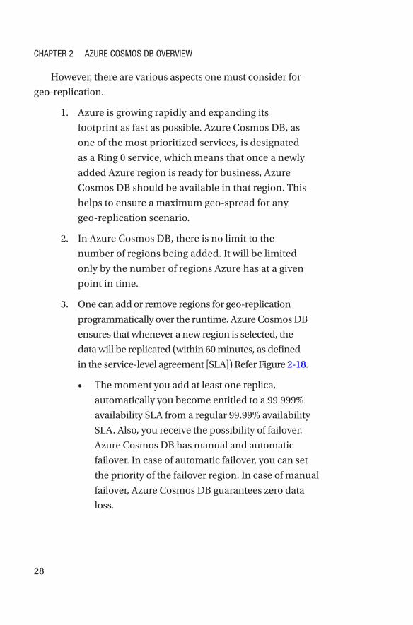
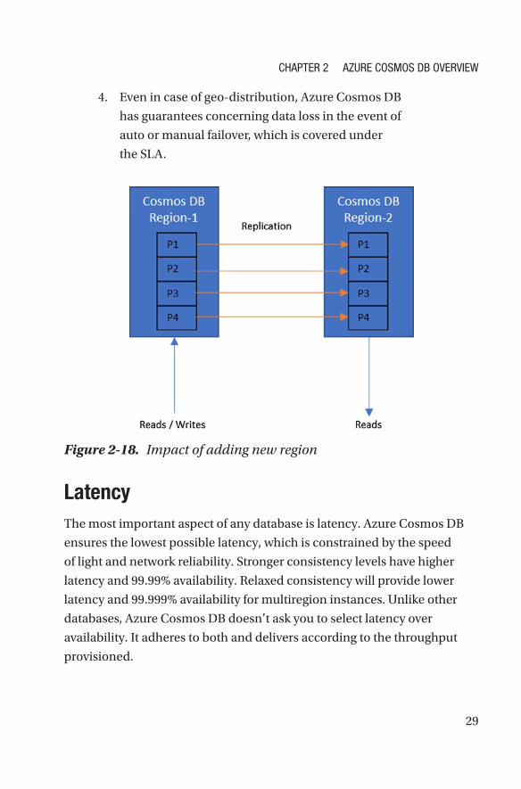
3. One can add or remove regions for geo-replication
programmatically over the runtime. Azure Cosmos DB
ensures that whenever a new region is selected, the
data will be replicated (within 60 minutes, as defined
in the service-level agreement [SLA]) Refer Figure 2-18.
• The moment you add at least one replica,
automatically you become entitled to a 99.999%
availability SLA from a regular 99.99% availability
SLA. Also, you receive the possibility of failover.
Azure Cosmos DB has manual and automatic
failover. In case of automatic failover, you can set
the priority of the failover region. In case of manual
failover, Azure Cosmos DB guarantees zero data
loss.
Chapter 2 azure Cosmos DB overview
29
4. Even in case of geo-distribution, Azure Cosmos DB
has guarantees concerning data loss in the event of
auto or manual failover, which is covered under
the SLA.
LatencyThe most important aspect of any database is latency. Azure Cosmos DB
ensures the lowest possible latency, which is constrained by the speed
of light and network reliability. Stronger consistency levels have higher
latency and 99.99% availability. Relaxed consistency will provide lower
latency and 99.999% availability for multiregion instances. Unlike other
databases, Azure Cosmos DB doesn’t ask you to select latency over
availability. It adheres to both and delivers according to the throughput
provisioned.
Figure 2-18. Impact of adding new region
Chapter 2 azure Cosmos DB overview
30
ConsistencyThis is a very critical aspect of the database and can affect its quality.
Let’s say if one has selected a certain level of consistency and enables the
geo-replication, there could be a concern over how Azure Cosmos DB will
guarantee it. To address that concern, let’s look at the implementation
closely. It is proven by the CAP theorem that it is impossible for a system
to maintain consistency and availability in cases of failures. Hence, the
system could be either CP (consistency and partition tolerant) or AP
(availability and partition tolerant). The Azure Cosmos DB adheres to
consistency, which makes it CP.
ThroughputAzure Cosmos DB scales infinitely and ensures predictable throughput. To
scale it would require a partition key, which will segregate the data into a
logical/physical partition, which is completely managed by Azure Cosmos
DB. Based on the consistency level partition set, it will be configured
dynamically, using different topologies (e.g., start, daisy chain, tree, etc.).
In the case of geo-replication, the partition key plays a major role, as each
partition set will be distributed across multiple regions.
AvailabilityAzure Cosmos DB offers an availability of 99.99% (a possible unavailability
of 52 minutes, 35.7 seconds a year) for a single region and 99.999% (a
possible unavailability of 5 minutes, 15.6 seconds a year) availability for
multiregions. It ensures availability by considering the upper boundary
of latency on every operation, which doesn’t change when you add a
new replica or have many replicas. It doesn’t matter whether manual
failover is applied or automatic failover is called. The term multi-homing
Chapter 2 azure Cosmos DB overview
31
API (application programming interface) describes failovers transparent
to the application that don’t require the application to be redeployed or
configured after the failover occurs.
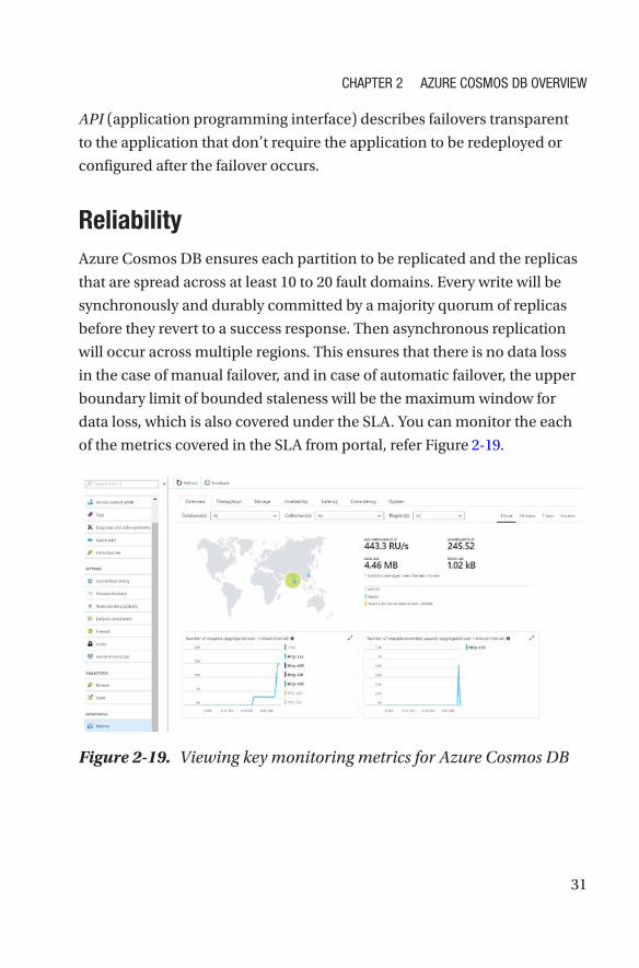
ReliabilityAzure Cosmos DB ensures each partition to be replicated and the replicas
that are spread across at least 10 to 20 fault domains. Every write will be
synchronously and durably committed by a majority quorum of replicas
before they revert to a success response. Then asynchronous replication
will occur across multiple regions. This ensures that there is no data loss
in the case of manual failover, and in case of automatic failover, the upper
boundary limit of bounded staleness will be the maximum window for
data loss, which is also covered under the SLA. You can monitor the each
of the metrics covered in the SLA from portal, refer Figure 2-19.
Figure 2-19. Viewing key monitoring metrics for Azure Cosmos DB
Chapter 2 azure Cosmos DB overview
32
Protocol Support and Multimodal APIAzure Cosmos DB provides multimodal API, which helps developers to
migrate from various NoSQL databases to Azure Cosmos DB, without
changing their application’s code. Currently, Cosmos DB supports SQL
API, MongoDB, Cassandra, Gremlin, and Azure Table Storage API.
In addition to API support, Azure Cosmos DB provides multimodel
implementation. This means that you can store data in various structures,
i.e., document, key-value, columnar, and graph.
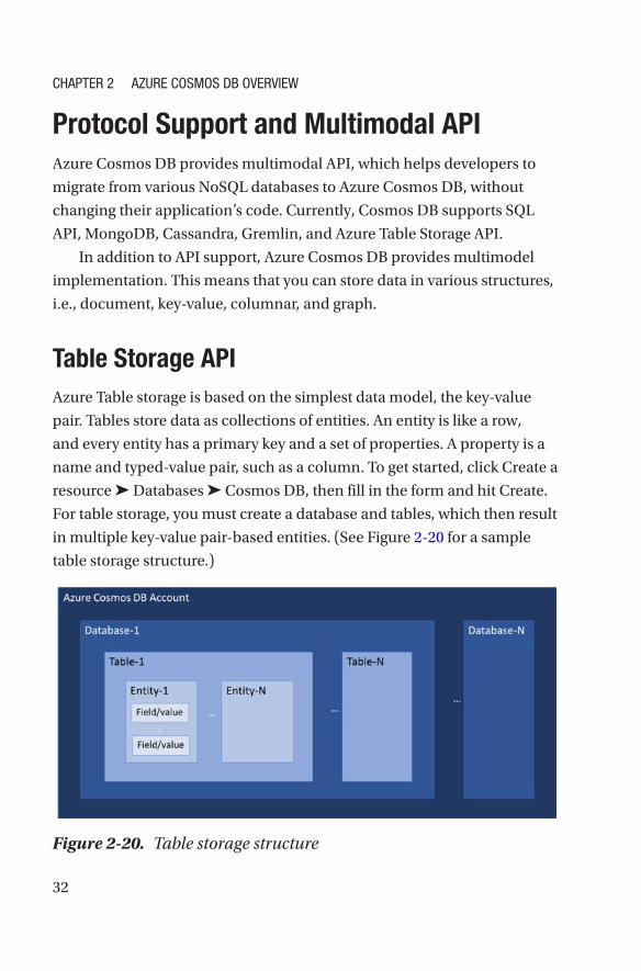
Table Storage APIAzure Table storage is based on the simplest data model, the key-value
pair. Tables store data as collections of entities. An entity is like a row,
and every entity has a primary key and a set of properties. A property is a
name and typed-value pair, such as a column. To get started, click Create a
resource ➤ Databases ➤ Cosmos DB, then fill in the form and hit Create.
For table storage, you must create a database and tables, which then result
in multiple key-value pair-based entities. (See Figure 2-20 for a sample
table storage structure.)
Figure 2-20. Table storage structure
Chapter 2 azure Cosmos DB overview
33
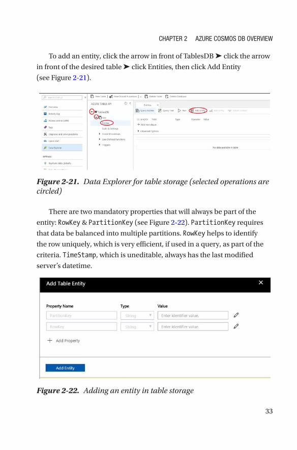
To add an entity, click the arrow in front of TablesDB ➤ click the arrow
in front of the desired table ➤ click Entities, then click Add Entity
(see Figure 2-21).
There are two mandatory properties that will always be part of the
entity: RowKey & PartitionKey (see Figure 2-22). PartitionKey requires
that data be balanced into multiple partitions. RowKey helps to identify
the row uniquely, which is very efficient, if used in a query, as part of the
criteria. TimeStamp, which is uneditable, always has the last modified
server’s datetime.
Figure 2-21. Data Explorer for table storage (selected operations are circled)
Figure 2-22. Adding an entity in table storage
Chapter 2 azure Cosmos DB overview
34
One can also use .NET, JAVA, NodeJs, Python, F#, C++, Ruby, or REST
API to interact with TableStorage API.
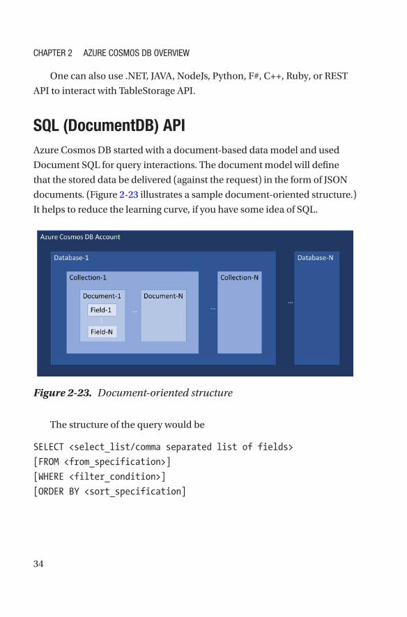
SQL (DocumentDB) APIAzure Cosmos DB started with a document-based data model and used
Document SQL for query interactions. The document model will define
that the stored data be delivered (against the request) in the form of JSON
documents. (Figure 2-23 illustrates a sample document-oriented structure.)
It helps to reduce the learning curve, if you have some idea of SQL.
The structure of the query would be
SELECT <select_list/comma separated list of fields>
[FROM <from_specification>]
[WHERE <filter_condition>]
[ORDER BY <sort_specification]
Figure 2-23. Document-oriented structure
Chapter 2 azure Cosmos DB overview
35
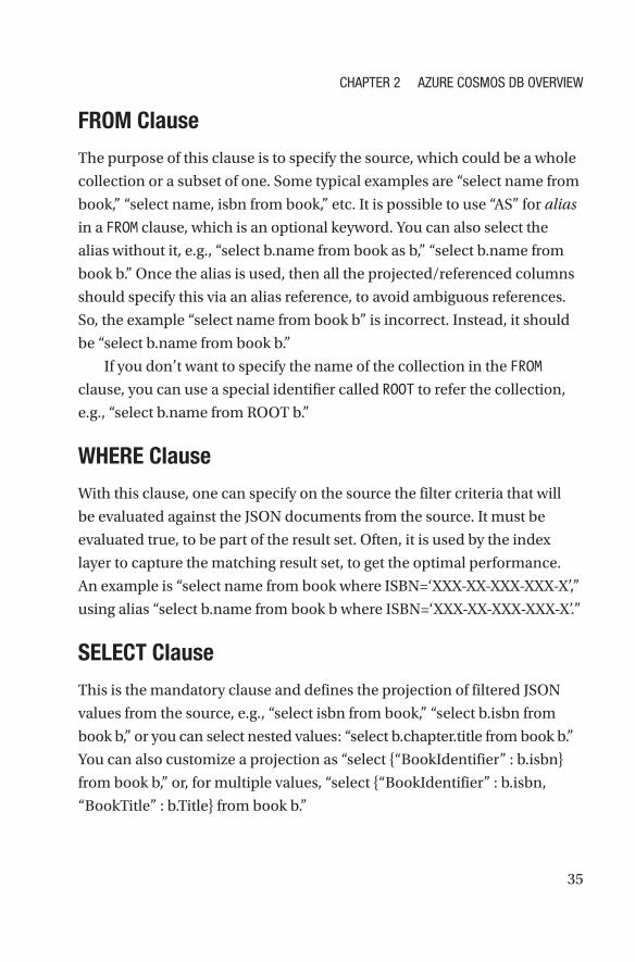
FROM Clause
The purpose of this clause is to specify the source, which could be a whole
collection or a subset of one. Some typical examples are “select name from
book,” “select name, isbn from book,” etc. It is possible to use “AS” for alias
in a FROM clause, which is an optional keyword. You can also select the
alias without it, e.g., “select b.name from book as b,” “select b.name from
book b.” Once the alias is used, then all the projected/referenced columns
should specify this via an alias reference, to avoid ambiguous references.
So, the example “select name from book b” is incorrect. Instead, it should
be “select b.name from book b.”
If you don’t want to specify the name of the collection in the FROM
clause, you can use a special identifier called ROOT to refer the collection,
e.g., “select b.name from ROOT b.”
WHERE Clause
With this clause, one can specify on the source the filter criteria that will
be evaluated against the JSON documents from the source. It must be
evaluated true, to be part of the result set. Often, it is used by the index
layer to capture the matching result set, to get the optimal performance.
An example is “select name from book where ISBN=‘XXX-XX-XXX-XXX-X’,”
using alias “select b.name from book b where ISBN=‘XXX-XX-XXX-XXX-X’.”
SELECT Clause
This is the mandatory clause and defines the projection of filtered JSON
values from the source, e.g., “select isbn from book,” “select b.isbn from
book b,” or you can select nested values: “select b.chapter.title from book b.”
You can also customize a projection as “select {“BookIdentifier” : b.isbn}
from book b,” or, for multiple values, “select {“BookIdentifier” : b.isbn,
“BookTitle” : b.Title} from book b.”
Chapter 2 azure Cosmos DB overview
36
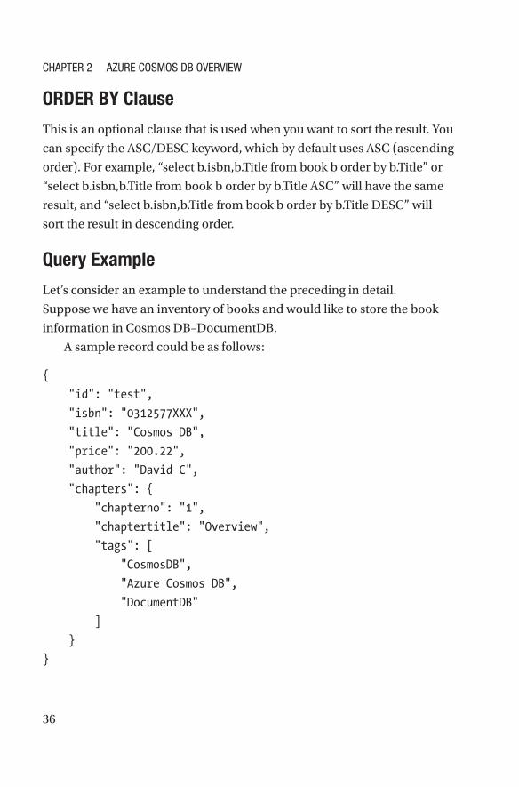
ORDER BY Clause
This is an optional clause that is used when you want to sort the result. You
can specify the ASC/DESC keyword, which by default uses ASC (ascending
order). For example, “select b.isbn,b.Title from book b order by b.Title” or
“select b.isbn,b.Title from book b order by b.Title ASC” will have the same
result, and “select b.isbn,b.Title from book b order by b.Title DESC” will
sort the result in descending order.
Query Example
Let’s consider an example to understand the preceding in detail.
Suppose we have an inventory of books and would like to store the book
information in Cosmos DB–DocumentDB.
A sample record could be as follows:
{
"id": "test",
"isbn": "0312577XXX",
"title": "Cosmos DB",
"price": "200.22",
"author": "David C",
"chapters": {
"chapterno": "1",
"chaptertitle": "Overview",
"tags": [
"CosmosDB",
"Azure Cosmos DB",
"DocumentDB"
]
}
}
Chapter 2 azure Cosmos DB overview
37
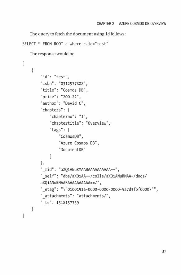
The query to fetch the document using id follows:
SELECT * FROM ROOT c where c.id="test"
The response would be
[
{
"id": "test",
"isbn": "0312577XXX",
"title": "Cosmos DB",
"price": "200.22",
"author": "David C",
"chapters": {
"chapterno": "1",
"chaptertitle": "Overview",
"tags": [
"CosmosDB",
"Azure Cosmos DB",
"DocumentDB"
]
},
"_rid": "aXQ1ANuRMAABAAAAAAAAAA==",
"_self": "dbs/aXQ1AA==/colls/aXQ1ANuRMAA=/docs/
aXQ1ANuRMAABAAAAAAAAAA==/",
"_etag": "\"0100191a-0000-0000-0000-5a7d3fbf0000\"",
"_attachments": "attachments/",
"_ts": 1518157759
}
]
Chapter 2 azure Cosmos DB overview
38
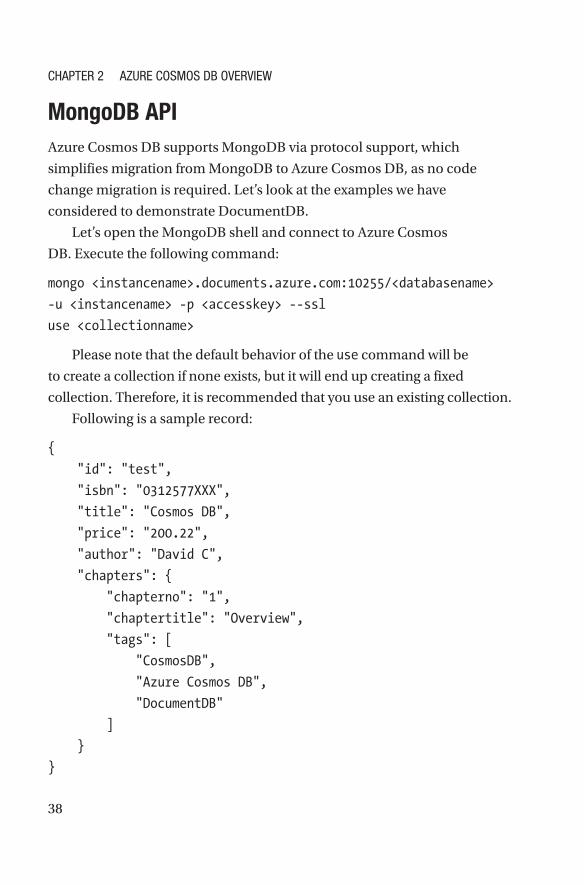
MongoDB API Azure Cosmos DB supports MongoDB via protocol support, which
simplifies migration from MongoDB to Azure Cosmos DB, as no code
change migration is required. Let’s look at the examples we have
considered to demonstrate DocumentDB.
Let’s open the MongoDB shell and connect to Azure Cosmos
DB. Execute the following command:
mongo <instancename>.documents.azure.com:10255/<databasename>
-u <instancename> -p <accesskey> --ssl
use <collectionname>
Please note that the default behavior of the use command will be
to create a collection if none exists, but it will end up creating a fixed
collection. Therefore, it is recommended that you use an existing collection.
Following is a sample record:
{
"id": "test",
"isbn": "0312577XXX",
"title": "Cosmos DB",
"price": "200.22",
"author": "David C",
"chapters": {
"chapterno": "1",
"chaptertitle": "Overview",
"tags": [
"CosmosDB",
"Azure Cosmos DB",
"DocumentDB"
]
}
}
Chapter 2 azure Cosmos DB overview
39
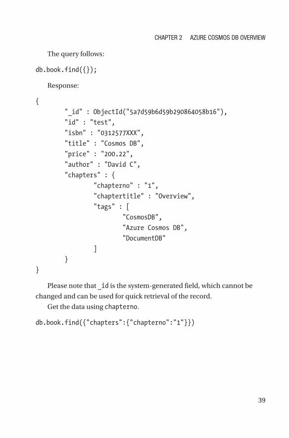
The query follows:
db.book.find({});
Response:
{
"_id" : ObjectId("5a7d59b6d59b290864058b16"),
"id" : "test",
"isbn" : "0312577XXX",
"title" : "Cosmos DB",
"price" : "200.22",
"author" : "David C",
"chapters" : {
"chapterno" : "1",
"chaptertitle" : "Overview",
"tags" : [
"CosmosDB",
"Azure Cosmos DB",
"DocumentDB"
]
}
}
Please note that _id is the system-generated field, which cannot be
changed and can be used for quick retrieval of the record.
Get the data using chapterno.
db.book.find({"chapters":{"chapterno":"1"}})
Chapter 2 azure Cosmos DB overview
40
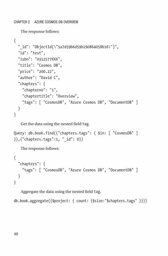
The response follows:
{
"_id": "ObjectId(\"5a7d59b6d59b290864058b16\")",
"id": "test",
"isbn": "0312577XXX",
"title": "Cosmos DB",
"price": "200.22",
"author": "David C",
"chapters": {
"chapterno": "1",
"chaptertitle": "Overview",
"tags": [ "CosmosDB", "Azure Cosmos DB", "DocumentDB" ]
}
}
Get the data using the nested field tag.
Query: db.book.find({"chapters.tags": { $in: [ "CosmosDB" ]
}},{"chapters.tags":1, "_id": 0})
The response follows:
{
"chapters": {
"tags": [ "CosmosDB", "Azure Cosmos DB", "DocumentDB" ]
}
}
Aggregate the data using the nested field tag.
db.book.aggregate({$project: { count: {$size:"$chapters.tags" }}})
Chapter 2 azure Cosmos DB overview
41
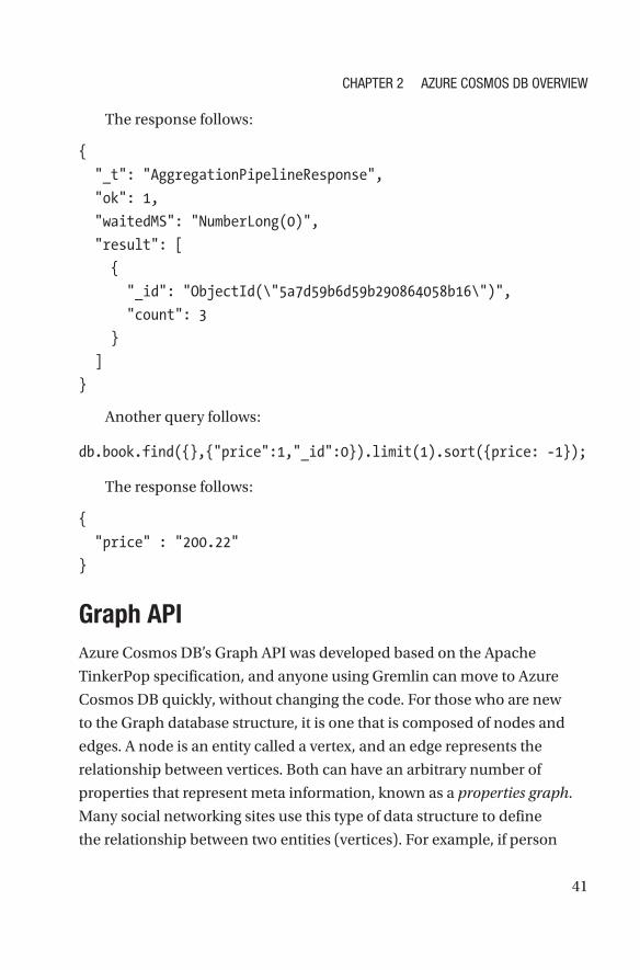
The response follows:
{
"_t": "AggregationPipelineResponse",
"ok": 1,
"waitedMS": "NumberLong(0)",
"result": [
{
"_id": "ObjectId(\"5a7d59b6d59b290864058b16\")",
"count": 3
}
]
}
Another query follows:
db.book.find({},{"price":1,"_id":0}).limit(1).sort({price: -1});
The response follows:
{
"price" : "200.22"
}
Graph APIAzure Cosmos DB’s Graph API was developed based on the Apache
TinkerPop specification, and anyone using Gremlin can move to Azure
Cosmos DB quickly, without changing the code. For those who are new
to the Graph database structure, it is one that is composed of nodes and
edges. A node is an entity called a vertex, and an edge represents the
relationship between vertices. Both can have an arbitrary number of
properties that represent meta information, known as a properties graph.
Many social networking sites use this type of data structure to define
the relationship between two entities (vertices). For example, if person
Chapter 2 azure Cosmos DB overview
42
A knows person B, wherein person A and person B are the vertex, the
relationship “knows” will be the edge. Person A can have a name, age,
and address as properties, and the edge can have properties such as
commonInterest, etc.
The Azure Cosmos DB Graph API uses the GraphSON format for
returning the result. It is the standard Gremlin format with which to
represent vertices, edges, and properties, using JSON.
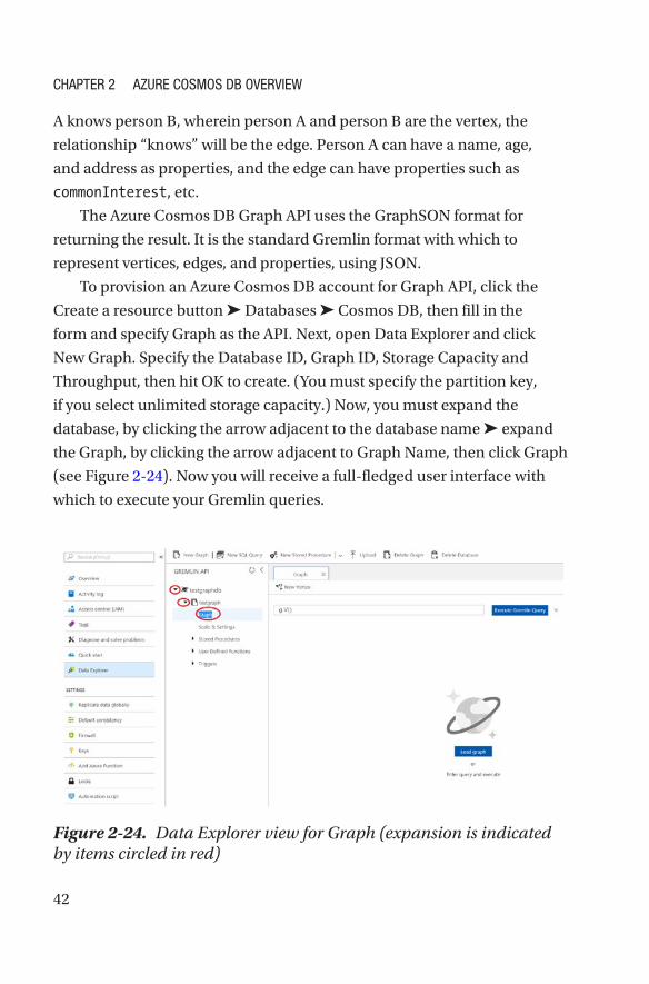
To provision an Azure Cosmos DB account for Graph API, click the
Create a resource button ➤ Databases ➤ Cosmos DB, then fill in the
form and specify Graph as the API. Next, open Data Explorer and click
New Graph. Specify the Database ID, Graph ID, Storage Capacity and
Throughput, then hit OK to create. (You must specify the partition key,
if you select unlimited storage capacity.) Now, you must expand the
database, by clicking the arrow adjacent to the database name ➤ expand
the Graph, by clicking the arrow adjacent to Graph Name, then click Graph
(see Figure 2-24). Now you will receive a full-fledged user interface with
which to execute your Gremlin queries.
Figure 2-24. Data Explorer view for Graph (expansion is indicated by items circled in red)
Chapter 2 azure Cosmos DB overview
43
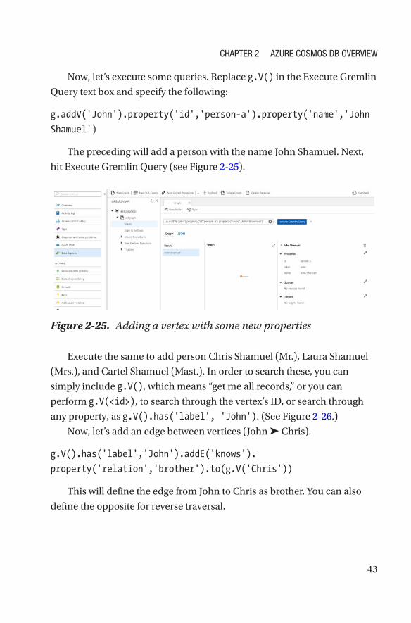
Now, let’s execute some queries. Replace g.V() in the Execute Gremlin
Query text box and specify the following:
g.addV('John').property('id','person-a').property('name','John
Shamuel')
The preceding will add a person with the name John Shamuel. Next,
hit Execute Gremlin Query (see Figure 2-25).
Figure 2-25. Adding a vertex with some new properties
Execute the same to add person Chris Shamuel (Mr.), Laura Shamuel
(Mrs.), and Cartel Shamuel (Mast.). In order to search these, you can
simply include g.V(), which means “get me all records,” or you can
perform g.V(<id>), to search through the vertex’s ID, or search through
any property, as g.V().has('label', 'John'). (See Figure 2-26.)
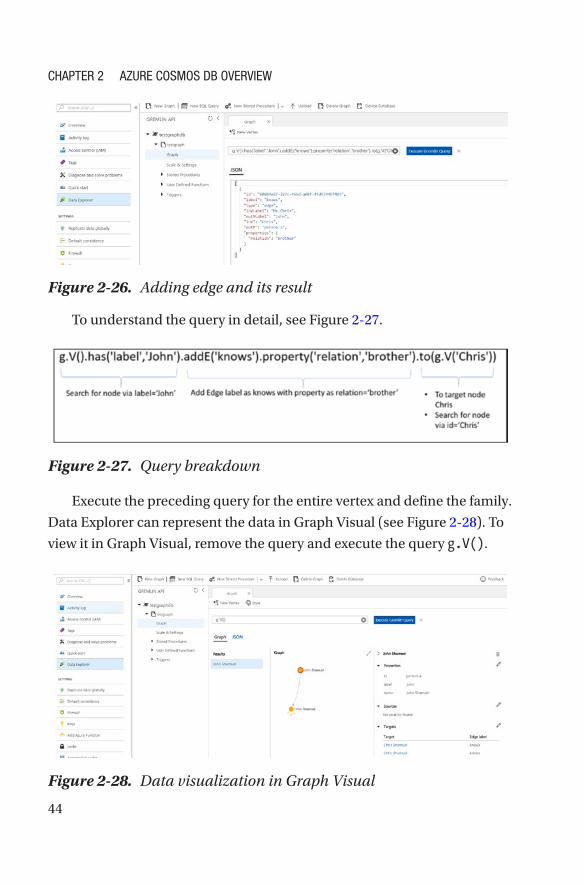
Now, let’s add an edge between vertices (John ➤ Chris).
g.V().has('label','John').addE('knows').
property('relation','brother').to(g.V('Chris'))
This will define the edge from John to Chris as brother. You can also
define the opposite for reverse traversal.
Chapter 2 azure Cosmos DB overview
44
To understand the query in detail, see Figure 2-27.
Execute the preceding query for the entire vertex and define the family.
Data Explorer can represent the data in Graph Visual (see Figure 2-28). To
view it in Graph Visual, remove the query and execute the query g.V().
Figure 2-26. Adding edge and its result
Figure 2-27. Query breakdown
Figure 2-28. Data visualization in Graph Visual
Chapter 2 azure Cosmos DB overview
45
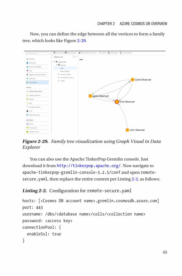
Now, you can define the edge between all the vertices to form a family
tree, which looks like Figure 2-29.
Figure 2-29. Family tree visualization using Graph Visual in Data Explorer
You can also use the Apache TinkerPop Gremlin console. Just
download it from http://tinkerpop.apache.org/. Now navigate to
apache-tinkerpop-gremlin-console-3.2.5/conf and open remote-
secure.yaml, then replace the entire content per Listing 2-2, as follows:
Listing 2-2. Configuration for remote-secure.yaml
hosts: [<Cosmos DB account name>.gremlin.cosmosdb.azure.com]
port: 443
username: /dbs/<database name>/colls/<collection name>
password: <access key>
connectionPool: {
enableSsl: true
}
Chapter 2 azure Cosmos DB overview
46
serializer: { className: org.apache.tinkerpop.gremlin.
driver.ser.GraphSONMessageSerializerV1d0, config: {
serializeResultToString: true }}
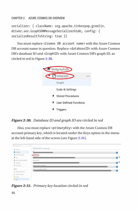
You must replace <Cosmos DB account name> with the Azure Cosmos
DB account name in question. Replace <databaseID> with Azure Cosmos
DB’s database ID and <GraphID> with Azure Cosmos DB’s graph ID, as
circled in red in Figure 2-30.
Figure 2-30. Database ID and graph ID are circled in red
Figure 2-31. Primary key location circled in red
Also, you must replace <primaryKey> with the Azure Cosmos DB
account primary key, which is located under the Keys option in the menu
at the left-hand side of the screen (see Figure 2-31).
Chapter 2 azure Cosmos DB overview
47
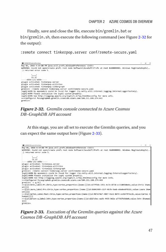
Finally, save and close the file, execute bin/gremlin.bat or
bin/gremlin.sh, then execute the following command (see Figure 2-32 for
the output):
:remote connect tinkerpop.server conf/remote-secure.yaml
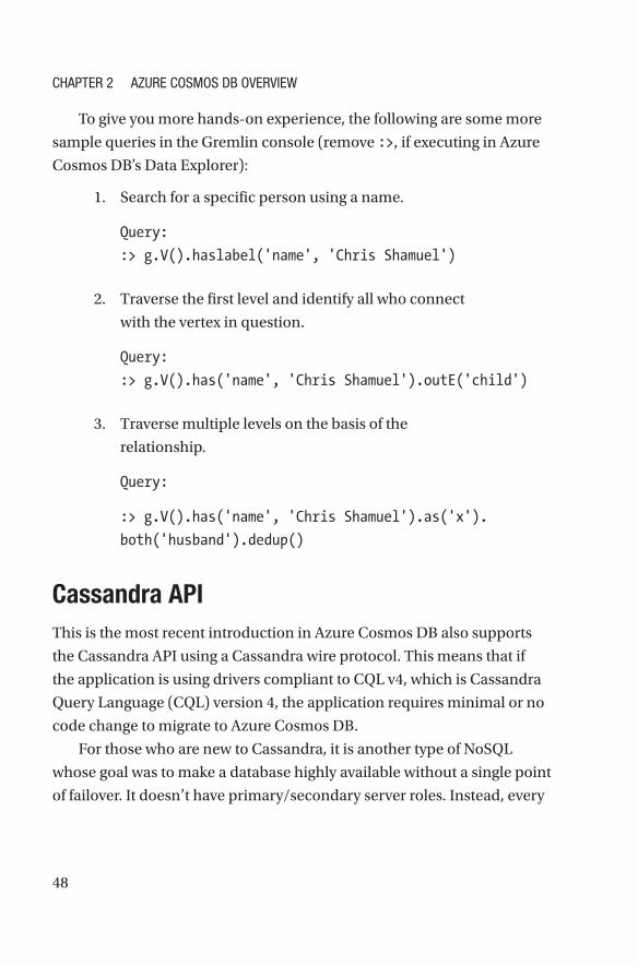
At this stage, you are all set to execute the Gremlin queries, and you
can expect the same output here (Figure 2-33).
Figure 2-32. Gremlin console connected to Azure Cosmos DB–GraphDB API account
Figure 2-33. Execution of the Gremlin queries against the Azure Cosmos DB–GraphDB API account
Chapter 2 azure Cosmos DB overview
48
To give you more hands-on experience, the following are some more
sample queries in the Gremlin console (remove :>, if executing in Azure
Cosmos DB’s Data Explorer):
1. Search for a specific person using a name.
Query:
:> g.V().haslabel('name', 'Chris Shamuel')
2. Traverse the first level and identify all who connect
with the vertex in question.
Query:
:> g.V().has('name', 'Chris Shamuel').outE('child')
3. Traverse multiple levels on the basis of the
relationship.
Query:
:> g.V().has('name', 'Chris Shamuel').as('x').
both('husband').dedup()
Cassandra APIThis is the most recent introduction in Azure Cosmos DB also supports
the Cassandra API using a Cassandra wire protocol. This means that if
the application is using drivers compliant to CQL v4, which is Cassandra
Query Language (CQL) version 4, the application requires minimal or no
code change to migrate to Azure Cosmos DB.
For those who are new to Cassandra, it is another type of NoSQL
whose goal was to make a database highly available without a single point
of failover. It doesn’t have primary/secondary server roles. Instead, every
Chapter 2 azure Cosmos DB overview
49
server is equivalent and has the capability to add or remove nodes over the
runtime. While writing the book, this API was just being announced and
was not available publicly.
Elastic ScaleAzure Cosmos DB is infinitely scalable, without losing latency. Scaling has
two variables: throughput and storage. Cosmos DB can scale using both,
and the best part is that there is no need to club these together, so scaling
can be done independent of other parameters.
ThroughputIncreasing compute throughput is easy. One can navigate to the Azure
portal and increase request units (RUs) or use CLI to do it without any
downtime. In case more compute throughput is required, one can scale
up, or scale down, if less throughput is required, without any downtime.
Following is the Azure CLI command that can be used to scale the
throughput:
az cosmosdb collection update --collection-name $collectionName
--name $instanceName --db-name $databaseName --resource-group
$resourceGroupName --throughput $newThroughput
StorageAzure Cosmos DB provides two options to configure a collection. One is to
have limited storage (up to 10GB). The other is to have unlimited storage.
In case of unlimited storage, the distribution of data depends on the shard
key provided. I will discuss partitioning in detail later in Chapter 3.
Chapter 2 azure Cosmos DB overview
50
Following is the Azure CLI command that can be used to create a
collection with unlimited storage:
az cosmosdb collection create --collection-name 'mycollection
--name 'mycosmosdb' --db-name 'mydb' --resource-group
'samplerg' --throughput 11000 --partition-key-path '/pkey'
ConsistencyAzure Cosmos DB provides five levels of consistency: strong, bounded
staleness, session, consistent prefix, and eventual.
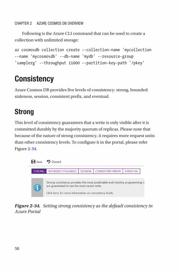
StrongThis level of consistency guarantees that a write is only visible after it is
committed durably by the majority quorum of replicas. Please note that
because of the nature of strong consistency, it requires more request units
than other consistency levels. To configure it in the portal, please refer
Figure 2-34.
Figure 2-34. Setting strong consistency as the default consistency in Azure Portal
Chapter 2 azure Cosmos DB overview
51
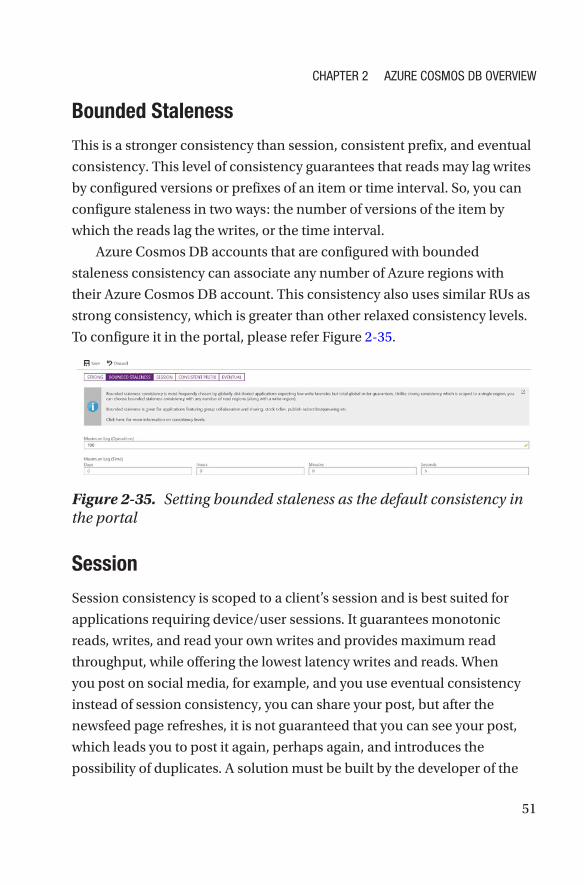
Bounded Staleness
This is a stronger consistency than session, consistent prefix, and eventual
consistency. This level of consistency guarantees that reads may lag writes
by configured versions or prefixes of an item or time interval. So, you can
configure staleness in two ways: the number of versions of the item by
which the reads lag the writes, or the time interval.
Azure Cosmos DB accounts that are configured with bounded
staleness consistency can associate any number of Azure regions with
their Azure Cosmos DB account. This consistency also uses similar RUs as
strong consistency, which is greater than other relaxed consistency levels.
To configure it in the portal, please refer Figure 2-35.
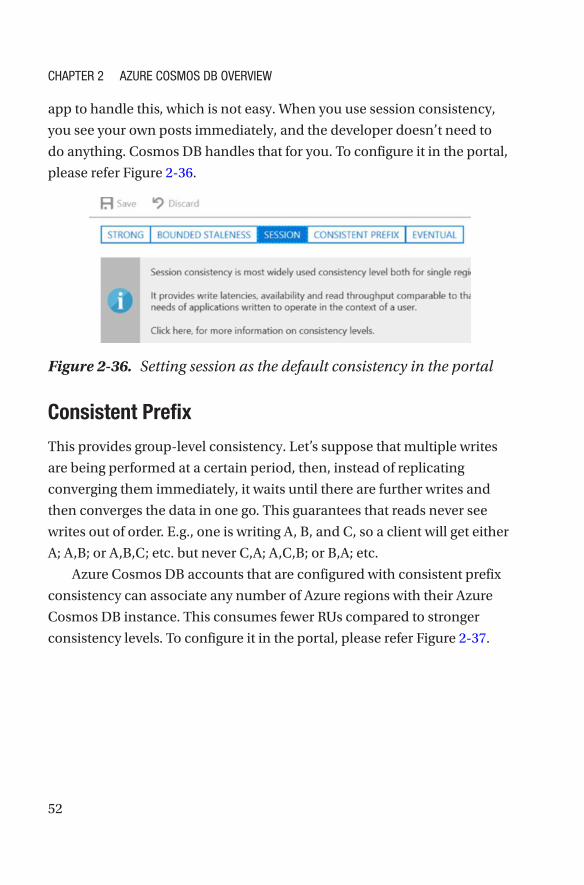
Session
Session consistency is scoped to a client’s session and is best suited for
applications requiring device/user sessions. It guarantees monotonic
reads, writes, and read your own writes and provides maximum read
throughput, while offering the lowest latency writes and reads. When
you post on social media, for example, and you use eventual consistency
instead of session consistency, you can share your post, but after the
newsfeed page refreshes, it is not guaranteed that you can see your post,
which leads you to post it again, perhaps again, and introduces the
possibility of duplicates. A solution must be built by the developer of the
Figure 2-35. Setting bounded staleness as the default consistency in the portal
Chapter 2 azure Cosmos DB overview
52
app to handle this, which is not easy. When you use session consistency,
you see your own posts immediately, and the developer doesn’t need to
do anything. Cosmos DB handles that for you. To configure it in the portal,
please refer Figure 2-36.
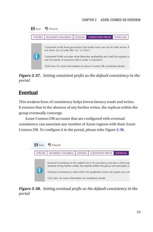
Consistent Prefix
This provides group-level consistency. Let’s suppose that multiple writes
are being performed at a certain period, then, instead of replicating
converging them immediately, it waits until there are further writes and
then converges the data in one go. This guarantees that reads never see
writes out of order. E.g., one is writing A, B, and C, so a client will get either
A; A,B; or A,B,C; etc. but never C,A; A,C,B; or B,A; etc.
Azure Cosmos DB accounts that are configured with consistent prefix
consistency can associate any number of Azure regions with their Azure
Cosmos DB instance. This consumes fewer RUs compared to stronger
consistency levels. To configure it in the portal, please refer Figure 2-37.
Figure 2-36. Setting session as the default consistency in the portal
Chapter 2 azure Cosmos DB overview
53
Figure 2-37. Setting consistent prefix as the default consistency in the portal
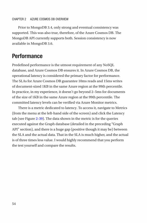
Eventual
This weakest form of consistency helps lowest latency reads and writes.
It ensures that in the absence of any further writes, the replicas within the
group eventually converge.
Azure Cosmos DB accounts that are configured with eventual
consistency can associate any number of Azure regions with their Azure
Cosmos DB. To configure it in the portal, please refer Figure 2-38.
Figure 2-38. Setting eventual prefix as the default consistency in the portal
Chapter 2 azure Cosmos DB overview
54
Prior to MongoDB 3.4, only strong and eventual consistency was
supported. This was also true, therefore, of the Azure Cosmos DB. The
MongoDB API currently supports both. Session consistency is now
available in MongoDB 3.6.
PerformancePredefined performance is the utmost requirement of any NoSQL
database, and Azure Cosmos DB ensures it. In Azure Cosmos DB, the
operational latency is considered the primary factor for performance.
The SLAs for Azure Cosmos DB guarantee 10ms reads and 15ms writes
of document-sized 1KB in the same Azure region at the 99th percentile.
In practice, in my experience, it doesn’t go beyond 2–5ms for documents
of the size of 1KB in the same Azure region at the 99th percentile. The
committed latency levels can be verified via Azure Monitor metrics.
There is a metric dedicated to latency. To access it, navigate to Metrics
(from the menu at the left-hand side of the screen) and click the Latency
tab (see Figure 2-39). The data shown in the metric is for the queries
executed against the Graph database (detailed in the preceding “Graph
API” section), and there is a huge gap (positive though it may be) between
the SLA and the actual data. That in the SLA is much higher, and the actual
is of three times less value. I would highly recommend that you perform
the test yourself and compare the results.
Chapter 2 azure Cosmos DB overview

55
If by doing so you note the example at P99 level, we were receiving the
latency under the commitment level.
Service Level Agreement (SLA)Azure Cosmos DB is an enterprise-grade NoSQL database. It covers, in
financial-backed SLAs, all the aspects I have explained so far. The SLAs are
categorized as follows.
Availability SLAAzure Cosmos DB provides availability to 99.99%, if configured with no
geo-replication, and provides 99.999%, if configured with a minimum of
one additional Azure region. In case something goes wrong on the read
region, there will be no impact on the other regions and no loss of data
available in any other region. However, in case something goes wrong on
the write region, there will be two options available for failover: manual
Figure 2-39. Outcome of 99th percentile latency test
Chapter 2 azure Cosmos DB overview

56
failover and automatic failover. In case of manual failover, the guarantee
for data loss is 100%, which means no data loss. and for automatic failover,
data loss is the upper bound of bounded staleness, which means the
data written to group and not replicated at the disaster. You can monitor
availability through one of the metrics, called Availability (see Figure 2-40).
To ensure durability of each instance of Azure Cosmos DB, each
partition will be replicated across at least 10–20 fault domains. I will
discuss how to ensure minimal or no impact in the application in
Chapter 3.
Throughput SLAAzure Cosmos DB generates the error “Throughput failed requests” when
the compute unit is consumed to the maximum configured. If in any case
it generates this error without reaching the upper limit, it is considered an
error rate and calculated against the number of requests made during an
hourly interval. The guarantee of such a case not happening is 99.99%. To
monitor the throughput in Azure Portal, navigate to Metrics ➤ Throughput
tab, refer Figure 2-41.
Figure 2-40. Azure Cosmos DB monitoring metrics for Availability
Chapter 2 azure Cosmos DB overview
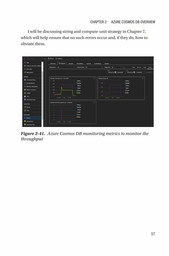
57
Figure 2-41. Azure Cosmos DB monitoring metrics to monitor the throughput
I will be discussing sizing and compute-unit strategy in Chapter 7,
which will help ensure that no such errors occur and, if they do, how to
obviate them.
Chapter 2 azure Cosmos DB overview
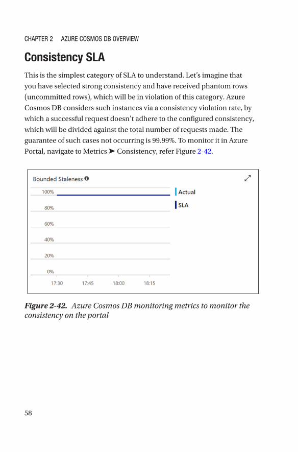
58
Figure 2-42. Azure Cosmos DB monitoring metrics to monitor the consistency on the portal
Consistency SLAThis is the simplest category of SLA to understand. Let’s imagine that
you have selected strong consistency and have received phantom rows
(uncommitted rows), which will be in violation of this category. Azure
Cosmos DB considers such instances via a consistency violation rate, by
which a successful request doesn’t adhere to the configured consistency,
which will be divided against the total number of requests made. The
guarantee of such cases not occurring is 99.99%. To monitor it in Azure
Portal, navigate to Metrics ➤ Consistency, refer Figure 2-42.
Chapter 2 azure Cosmos DB overview
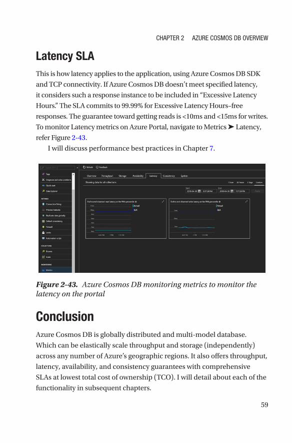
59
Figure 2-43. Azure Cosmos DB monitoring metrics to monitor the latency on the portal
Latency SLAThis is how latency applies to the application, using Azure Cosmos DB SDK
and TCP connectivity. If Azure Cosmos DB doesn’t meet specified latency,
it considers such a response instance to be included in “Excessive Latency
Hours.” The SLA commits to 99.99% for Excessive Latency Hours–free
responses. The guarantee toward getting reads is <10ms and <15ms for writes.
To monitor Latency metrics on Azure Portal, navigate to Metrics ➤ Latency,
refer Figure 2-43.
I will discuss performance best practices in Chapter 7.
ConclusionAzure Cosmos DB is globally distributed and multi-model database.
Which can be elastically scale throughput and storage (independently)
across any number of Azure’s geographic regions. It also offers throughput,
latency, availability, and consistency guarantees with comprehensive
SLAs at lowest total cost of ownership (TCO). I will detail about each of the
functionality in subsequent chapters.
Chapter 2 azure Cosmos DB overview
61© Manish Sharma 2018 M. Sharma, Cosmos DB for MongoDB Developers, https://doi.org/10.1007/978-1-4842-3682-6_3
CHAPTER 3
Azure Cosmos DB Geo-ReplicationAvailability of the database is of utmost importance to any application’s
experience. In cases where the user engagement is critical, and the
availability of the database in data-driven application is most important, one
must ensure the availability and scalability of the database. Among examples
of data-driven applications could be the following: an e-commerce
application with a plethora of easy-to-use and marquee features, going
down every time a user tries to make a purchase, because the database is
not available; a billing solution for a hospital that leaves patients standing in
line to make payments, owing to a database instance not being available; or
a transport company with footprints across the globe seeking to access the
system, but apart from that at the main location, the system performs badly,
owing to latency issues. So, how do you ensure that a database is available?
How do you ensure that the database is always deployed nearest to the
relevant application? And how do you achieve the lowest possible latency?
In this chapter, I will attempt to answer the queries related to database
availability. Also, I will go through Azure Cosmos DB’s global distribution
capability and discuss how it can help address availability challenges.
62
Database Availability (DA)To ensure database availability, we must ensure availability of the instance
running the database. We can achieve this by setting up high availability
(HA). This simply means that more than two instances should be running
a given workload. Running two or more instances of the same database
will be a tough job, as all the instances should be in sync, such that if one
instance goes offline, the second instance will be up and running, with
all the required data. This can be achieved by data replication, which is of
two types: master/slave and master/master. In the case of master/slave
data replication, there is one main database instance, which can perform
read and write transactions, and second or subsequent instances will
have a copy of the same data as the main instance but perform only read
transactions. In master/master replication, there is no main instance. All
the instances have equal privileges and can perform the read and write
transactions.
MongoDB ReplicationIn MongoDB, high availability (master/slave-based architecture) can be
configured via a replica set. In a replica set, data in the primary instance
will be replicated in secondary instances. The primary instance serves all
the write and read transactions, and the secondary node(s) serves read
transactions. The secondary nodes are further divided into two types:
data-bearing nodes and arbiter nodes. Let’s look at some of their
low-level details.
Data-Bearing NodesData-bearing nodes are those that carry the data set. All healthy data-
bearing nodes will continuously send pings to each other to check their
state of health. The replication of data from primary nodes occurs by
Chapter 3 azure Cosmos DB Geo-repliCation
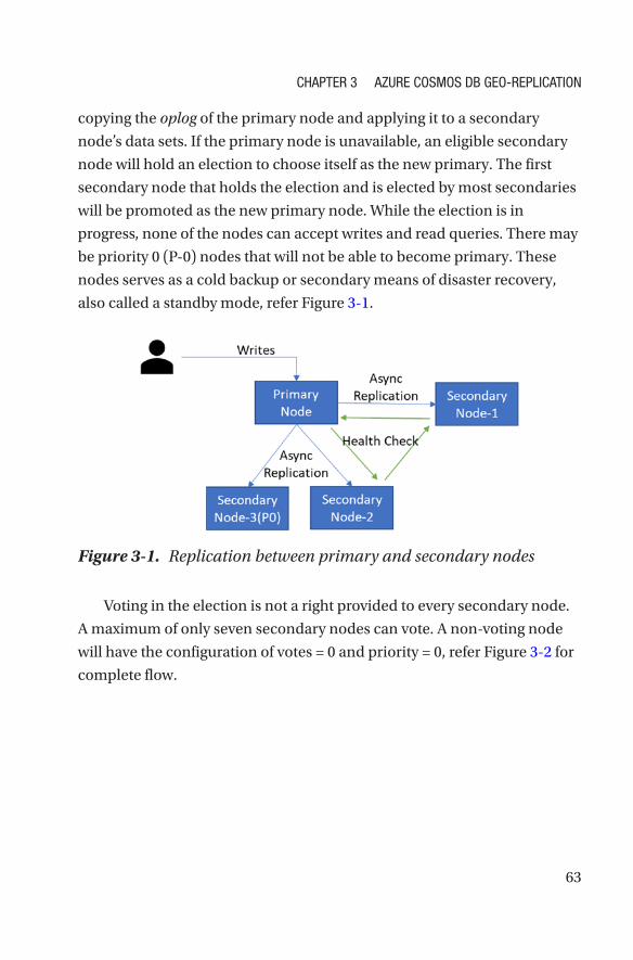
63
copying the oplog of the primary node and applying it to a secondary
node’s data sets. If the primary node is unavailable, an eligible secondary
node will hold an election to choose itself as the new primary. The first
secondary node that holds the election and is elected by most secondaries
will be promoted as the new primary node. While the election is in
progress, none of the nodes can accept writes and read queries. There may
be priority 0 (P-0) nodes that will not be able to become primary. These
nodes serves as a cold backup or secondary means of disaster recovery,
also called a standby mode, refer Figure 3-1.
Voting in the election is not a right provided to every secondary node.
A maximum of only seven secondary nodes can vote. A non-voting node
will have the configuration of votes = 0 and priority = 0, refer Figure 3-2 for
complete flow.
Figure 3-1. Replication between primary and secondary nodes
Chapter 3 azure Cosmos DB Geo-repliCation
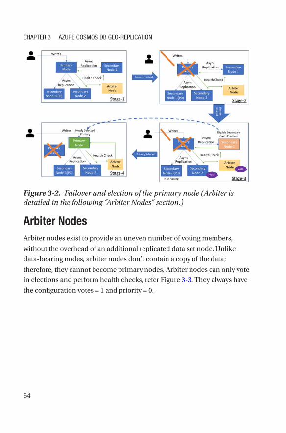
64
Arbiter NodesArbiter nodes exist to provide an uneven number of voting members,
without the overhead of an additional replicated data set node. Unlike
data-bearing nodes, arbiter nodes don’t contain a copy of the data;
therefore, they cannot become primary nodes. Arbiter nodes can only vote
in elections and perform health checks, refer Figure 3-3. They always have
the configuration votes = 1 and priority = 0.
Figure 3-2. Failover and election of the primary node (Arbiter is detailed in the following “Arbiter Nodes” section.)
Chapter 3 azure Cosmos DB Geo-repliCation
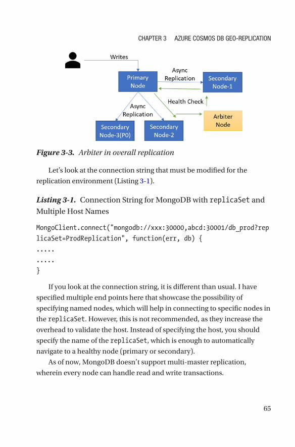
65
Let’s look at the connection string that must be modified for the
replication environment (Listing 3-1).
Listing 3-1. Connection String for MongoDB with replicaSet and
Multiple Host Names
MongoClient.connect("mongodb://xxx:30000,abcd:30001/db_prod?rep
licaSet=ProdReplication", function(err, db) {
.....
.....
}
If you look at the connection string, it is different than usual. I have
specified multiple end points here that showcase the possibility of
specifying named nodes, which will help in connecting to specific nodes in
the replicaSet. However, this is not recommended, as they increase the
overhead to validate the host. Instead of specifying the host, you should
specify the name of the replicaSet, which is enough to automatically
navigate to a healthy node (primary or secondary).
As of now, MongoDB doesn’t support multi-master replication,
wherein every node can handle read and write transactions.
Figure 3-3. Arbiter in overall replication
Chapter 3 azure Cosmos DB Geo-repliCation
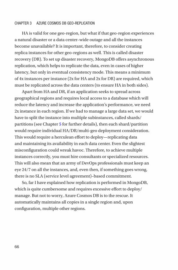
66
HA is valid for one geo-region, but what if that geo-region experiences
a natural disaster or a data center–wide outage and all the instances
become unavailable? It is important, therefore, to consider creating
replica instances for other geo-regions as well. This is called disaster
recovery (DR). To set up disaster recovery, MongoDB offers asynchronous
replication, which helps to replicate the data, even in cases of higher
latency, but only in eventual consistency mode. This means a minimum
of 4x instances per instance (2x for HA and 2x for DR) are required, which
must be replicated across the data centers (to ensure HA in both sides).
Apart from HA and DR, if an application seeks to spread across
geographical regions and requires local access to a database which will
reduce the latency and increase the application’s performance, we need
2x instance in each region. If we had to manage a large data set, we would
have to split the instance into multiple subinstances, called shards/
partitions (see Chapter 5 for further details), then each shard/partition
would require individual HA/DR/multi-geo deployment consideration.
This would require a herculean effort to deploy—replicating data
and maintaining its availability in each data center. Even the slightest
misconfiguration could wreak havoc. Therefore, to achieve multiple
instances correctly, you must hire consultants or specialized resources.
This will also mean that an army of DevOps professionals must keep an
eye 24/7 on all the instances, and, even then, if something goes wrong,
there is no SLA (service level agreement)–based commitment.
So, far I have explained how replication is performed in MongoDB,
which is quite cumbersome and requires excessive effort to deploy/
manage. But not to worry, Azure Cosmos DB is to the rescue. It
automatically maintains all copies in a single region and, upon
configuration, multiple other regions.
Chapter 3 azure Cosmos DB Geo-repliCation
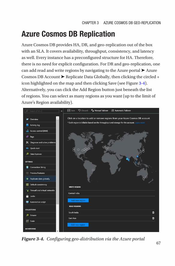
67
Azure Cosmos DB ReplicationAzure Cosmos DB provides HA, DR, and geo-replication out of the box
with an SLA. It covers availability, throughput, consistency, and latency
as well. Every instance has a preconfigured structure for HA. Therefore,
there is no need for explicit configuration. For DR and geo-replication, one
can add read and write regions by navigating to the Azure portal ➤ Azure
Cosmos DB Account ➤ Replicate Data Globally, then clicking the circled +
icon highlighted on the map and then clicking Save (see Figure 3-4).
Alternatively, you can click the Add Region button just beneath the list
of regions. You can select as many regions as you want (up to the limit of
Azure’s Region availability).
Figure 3-4. Configuring geo-distribution via the Azure portal
Chapter 3 azure Cosmos DB Geo-repliCation
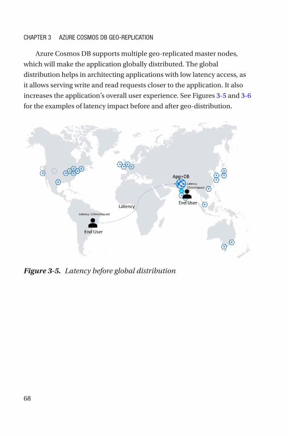
68
Azure Cosmos DB supports multiple geo-replicated master nodes,
which will make the application globally distributed. The global
distribution helps in architecting applications with low latency access, as
it allows serving write and read requests closer to the application. It also
increases the application’s overall user experience. See Figures 3-5 and 3-6
for the examples of latency impact before and after geo-distribution.
Figure 3-5. Latency before global distribution
Chapter 3 azure Cosmos DB Geo-repliCation
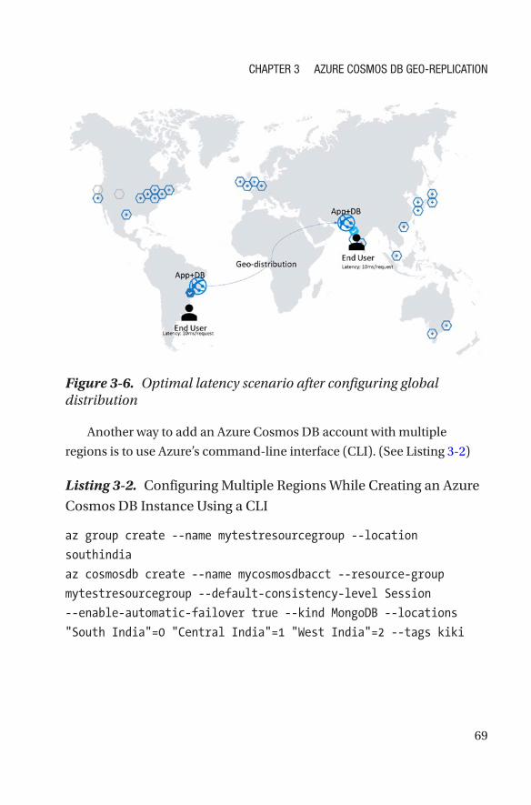
69
Another way to add an Azure Cosmos DB account with multiple
regions is to use Azure’s command-line interface (CLI). (See Listing 3-2)
Listing 3-2. Configuring Multiple Regions While Creating an Azure
Cosmos DB Instance Using a CLI
az group create --name mytestresourcegroup --location
southindia
az cosmosdb create --name mycosmosdbacct --resource-group
mytestresourcegroup --default-consistency-level Session
--enable-automatic-failover true --kind MongoDB --locations
"South India"=0 "Central India"=1 "West India"=2 --tags kiki
Figure 3-6. Optimal latency scenario after configuring global distribution
Chapter 3 azure Cosmos DB Geo-repliCation
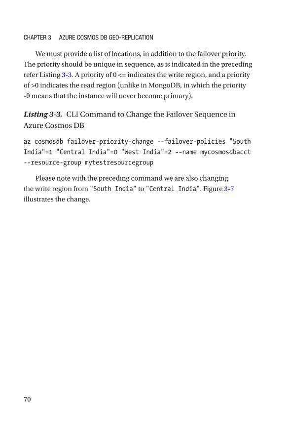
70
We must provide a list of locations, in addition to the failover priority.
The priority should be unique in sequence, as is indicated in the preceding
refer Listing 3-3. A priority of 0 <= indicates the write region, and a priority
of >0 indicates the read region (unlike in MongoDB, in which the priority
-0 means that the instance will never become primary).
Listing 3-3. CLI Command to Change the Failover Sequence in
Azure Cosmos DB
az cosmosdb failover-priority-change --failover-policies "South
India"=1 "Central India"=0 "West India"=2 --name mycosmosdbacct
--resource-group mytestresourcegroup
Please note with the preceding command we are also changing
the write region from "South India" to "Central India". Figure 3-7
illustrates the change.
Chapter 3 azure Cosmos DB Geo-repliCation
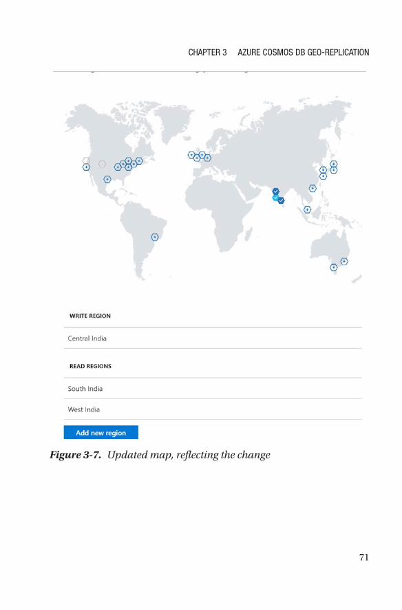
71
Figure 3-7. Updated map, reflecting the change
Chapter 3 azure Cosmos DB Geo-repliCation
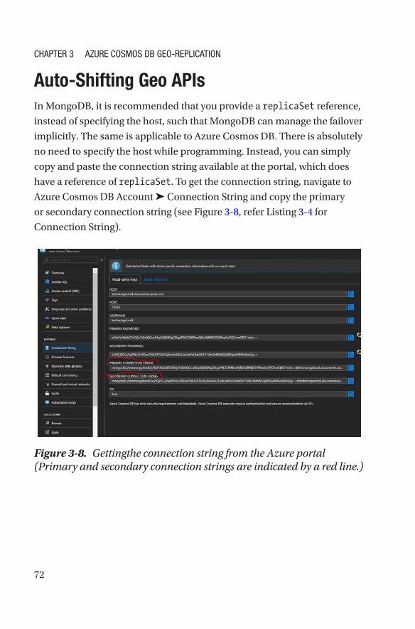
72
Auto-Shifting Geo APIsIn MongoDB, it is recommended that you provide a replicaSet reference,
instead of specifying the host, such that MongoDB can manage the failover
implicitly. The same is applicable to Azure Cosmos DB. There is absolutely
no need to specify the host while programming. Instead, you can simply
copy and paste the connection string available at the portal, which does
have a reference of replicaSet. To get the connection string, navigate to
Azure Cosmos DB Account ➤ Connection String and copy the primary
or secondary connection string (see Figure 3-8, refer Listing 3-4 for
Connection String).
Figure 3-8. Gettingthe connection string from the Azure portal (Primary and secondary connection strings are indicated by a red line.)
Chapter 3 azure Cosmos DB Geo-repliCation
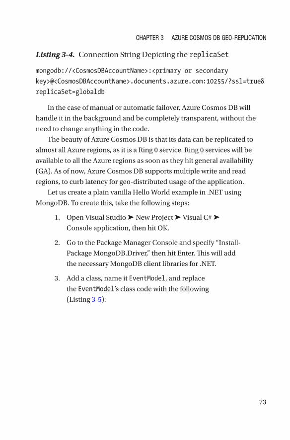
73
Listing 3-4. Connection String Depicting the replicaSet
mongodb://<CosmosDBAccountName>:<primary or secondary
key>@<CosmosDBAccountName>.documents.azure.com:10255/?ssl=true&
replicaSet=globaldb
In the case of manual or automatic failover, Azure Cosmos DB will
handle it in the background and be completely transparent, without the
need to change anything in the code.
The beauty of Azure Cosmos DB is that its data can be replicated to
almost all Azure regions, as it is a Ring 0 service. Ring 0 services will be
available to all the Azure regions as soon as they hit general availability
(GA). As of now, Azure Cosmos DB supports multiple write and read
regions, to curb latency for geo-distributed usage of the application.
Let us create a plain vanilla Hello World example in .NET using
MongoDB. To create this, take the following steps:
1. Open Visual Studio ➤ New Project ➤ Visual C# ➤
Console application, then hit OK.
2. Go to the Package Manager Console and specify “Install-
Package MongoDB.Driver,” then hit Enter. This will add
the necessary MongoDB client libraries for .NET.
3. Add a class, name it EventModel, and replace
the EventModel’s class code with the following
(Listing 3-5):
Chapter 3 azure Cosmos DB Geo-repliCation
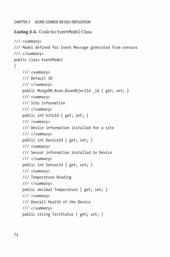
74
Listing 3-5. Code for EventModel Class
/// <summary>
/// Model defined for Event Message generated from sensors
/// </summary>
public class EventModel
{
/// <summary>
/// Default ID
/// </summary>
public MongoDB.Bson.BsonObjectId _id { get; set; }
/// <summary>
/// Site information
/// </summary>
public int SiteId { get; set; }
/// <summary>
/// Device information installed for a site
/// </summary>
public int DeviceId { get; set; }
/// <summary>
/// Sensor information installed in Device
/// </summary>
public int SensorId { get; set; }
/// <summary>
/// Temperature Reading
/// </summary>
public decimal Temperature { get; set; }
/// <summary>
/// Overall Health of the Device
/// </summary>
public string TestStatus { get; set; }
Chapter 3 azure Cosmos DB Geo-repliCation
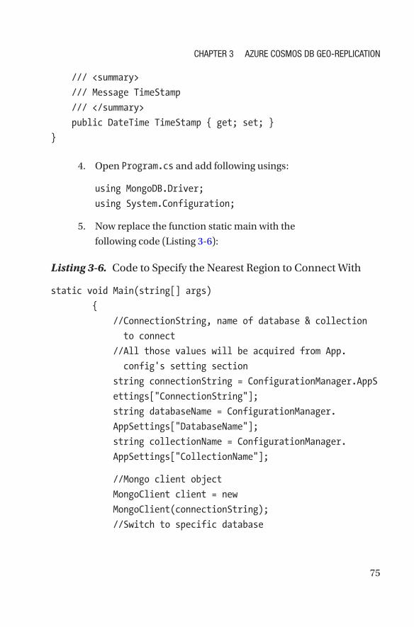
75
/// <summary>
/// Message TimeStamp
/// </summary>
public DateTime TimeStamp { get; set; }
}
4. Open Program.cs and add following usings:
using MongoDB.Driver;
using System.Configuration;
5. Now replace the function static main with the
following code (Listing 3-6):
Listing 3-6. Code to Specify the Nearest Region to Connect With
static void Main(string[] args)
{
// ConnectionString, name of database & collection
to connect
// All those values will be acquired from App.
config's setting section
string connectionString = ConfigurationManager.AppS
ettings["ConnectionString"];
string databaseName = ConfigurationManager.
AppSettings["DatabaseName"];
string collectionName = ConfigurationManager.
AppSettings["CollectionName"];
//Mongo client object
MongoClient client = new
MongoClient(connectionString);
//Switch to specific database
Chapter 3 azure Cosmos DB Geo-repliCation
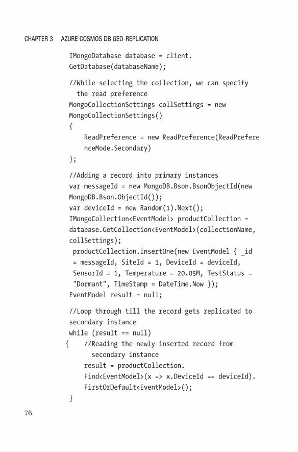
76
IMongoDatabase database = client.
GetDatabase(databaseName);
// While selecting the collection, we can specify
the read preference
MongoCollectionSettings collSettings = new
MongoCollectionSettings()
{
ReadPreference = new ReadPreference(ReadPrefere
nceMode.Secondary)
};
//Adding a record into primary instances
var messageId = new MongoDB.Bson.BsonObjectId(new
MongoDB.Bson.ObjectId());
var deviceId = new Random(1).Next();
IMongoCollection<EventModel> productCollection =
database.GetCollection<EventModel>(collectionName,
collSettings);
productCollection.InsertOne(new EventModel { _id
= messageId, SiteId = 1, DeviceId = deviceId,
SensorId = 1, Temperature = 20.05M, TestStatus =
"Dormant", TimeStamp = DateTime.Now });
EventModel result = null;
//Loop through till the record gets replicated to
secondary instance
while (result == null)
{ // Reading the newly inserted record from
secondary instance
result = productCollection.
Find<EventModel>(x => x.DeviceId == deviceId).
FirstOrDefault<EventModel>();
}
Chapter 3 azure Cosmos DB Geo-repliCation
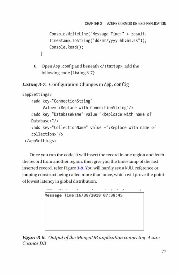
77
Console.WriteLine("Message Time:" + result.
TimeStamp.ToString("dd/mm/yyyy hh:mm:ss"));
Console.Read();
}
6. Open App.config and beneath </startup>, add the
following code (Listing 3-7):
Listing 3-7. Configuration Changes in App.config
<appSettings>
<add key="ConnectionString"
Value="<Replace with ConnectionString"/>
<add key="DatabaseName" value="<Replcace with name of
Database>"/>
<add key="CollectionName" value ="<Replace with name of
collection>"/>
</appSettings>
Once you run the code, it will insert the record in one region and fetch
the record from another region, then give you the timestamp of the last
inserted record, refer Figure 3-9. You will hardly see a NULL reference or
looping construct being called more than once, which will prove the point
of lowest latency in global distribution.
Figure 3-9. Output of the MongoDB application connecting Azure Cosmos DB
Chapter 3 azure Cosmos DB Geo-repliCation
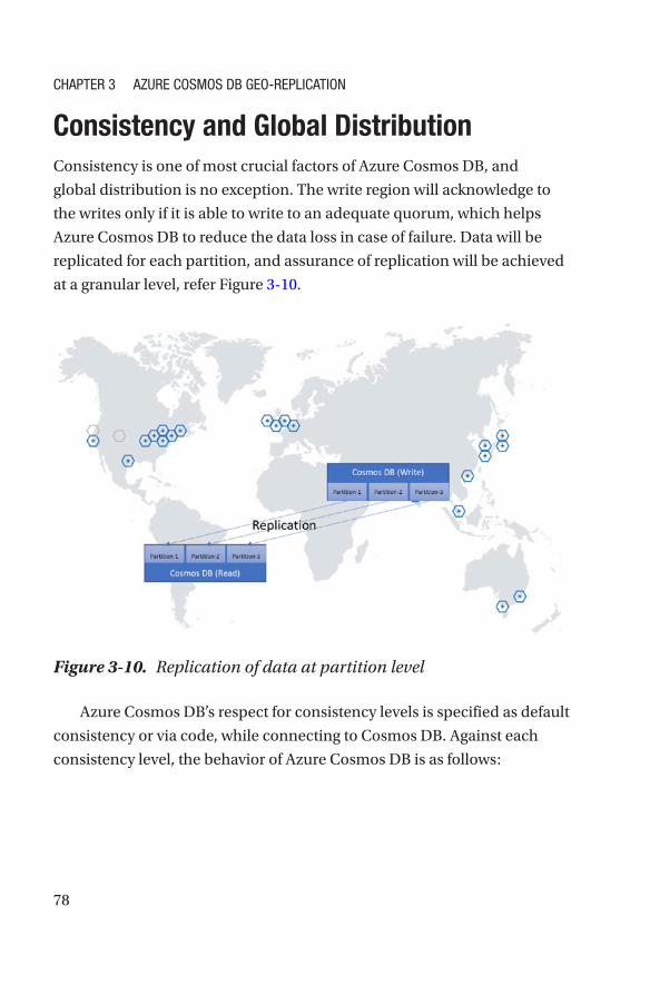
78
Consistency and Global DistributionConsistency is one of most crucial factors of Azure Cosmos DB, and
global distribution is no exception. The write region will acknowledge to
the writes only if it is able to write to an adequate quorum, which helps
Azure Cosmos DB to reduce the data loss in case of failure. Data will be
replicated for each partition, and assurance of replication will be achieved
at a granular level, refer Figure 3-10.
Azure Cosmos DB’s respect for consistency levels is specified as default
consistency or via code, while connecting to Cosmos DB. Against each
consistency level, the behavior of Azure Cosmos DB is as follows:
Figure 3-10. Replication of data at partition level
Chapter 3 azure Cosmos DB Geo-repliCation
79
• Strong consistency: The write region will acknowledge
this once it is able to write to all regions. It is one of the
costliest operations in terms of number of RUs being
consumed. In this case, the synchronous replication
increases the overall latency.
• Bounded staleness: This is preferred if you require
strong consistency with geo-replication. It will have a
lower cost impact compared to strong consistency on
writes. It will replicate the data async, and the time lag
will be equivalent to the specified interval. In the case
of automatic failover, the guarantee of data loss refers to
this interval.
• Session consistency: In this case, the scope of
consistency is limited to the user’s session, and
replication will be performed asynchronously.
• Consistent prefix: This is another form of eventual
consistency, except that it maintains the sequence of
writes during the replication.
• Eventual: This form of consistency is always the fastest
and cheapest, because the cost is less, and the latency
is lower.
ConclusionIn this chapter I have addressed various aspects of geo-replication in Azure
Cosmos DB and touched on various aspects that are specific to Azure
Cosmos DB. As we have seen through numerous examples, Azure Cosmos
DB–MongoDB API doesn’t introduce new jargon or syntax, which reduces
the learning curve during the migration from MongoDB. In subsequent
chapters, I will cover indexing, sizing, partition, and other key scenarios
that may refer to this chapter.
Chapter 3 azure Cosmos DB Geo-repliCation
81© Manish Sharma 2018 M. Sharma, Cosmos DB for MongoDB Developers, https://doi.org/10.1007/978-1-4842-3682-6_4
CHAPTER 4
IndexingIndexing is an inherent part of any database, so it is with MongoDB.
Indexing data is necessary to help reduce the scan overhead when finding
the values, for which there is a proverbial, “needle in a haystack.” In this
chapter, I will discuss how indexing works, indexing policies, possibilities
of customization, and indexing optimization.
Indexing in MongoDBIn MongoDB, users must define which path is to be indexed, and how.
This decision defines the performance of the query. However, indexes
have their own overhead. This creates a separate parallel tree structure
that consumes RAM, storage, and CPU while creating/updating/deleting
documents. Therefore, it’s important to make sure the maximum usage
of the index, but in practice, there might be some queries that don’t use
indexes. In such cases, MongoDB performs collection scans, which will
result in un-optimal performance. Such scenarios can be identified by
using the explain() method in MongoDB.
By default, MongoDB has an _id field with a unique index to identify
documents specifically. This unique index cannot be dropped. Distinct
types of indexes exist in MongoDB that serve different purposes, including
single field, compound, multikey, geospatial, text, and hashed indexes.
Let’s explore each of them.
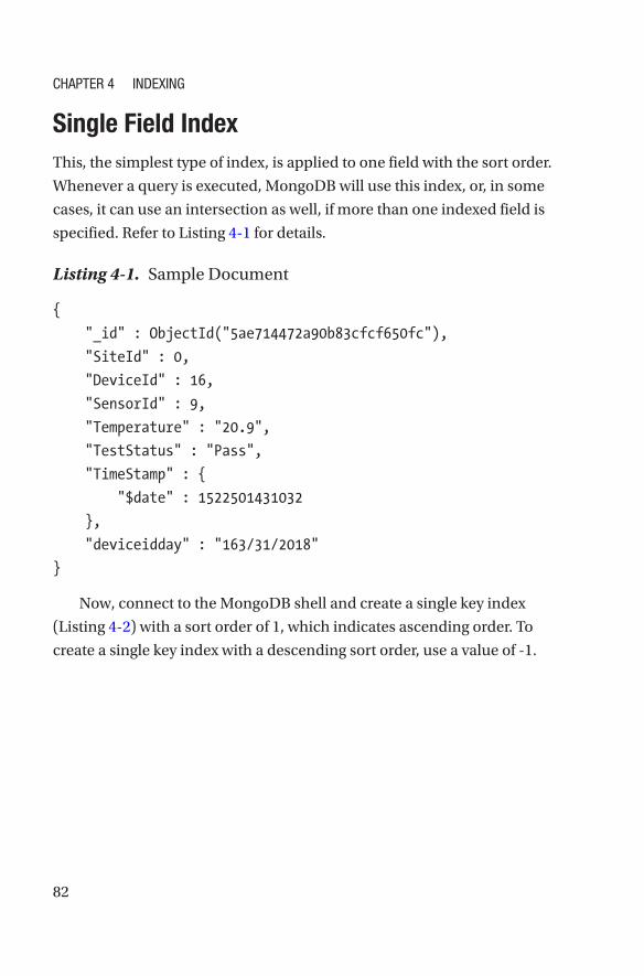
82
Single Field IndexThis, the simplest type of index, is applied to one field with the sort order.
Whenever a query is executed, MongoDB will use this index, or, in some
cases, it can use an intersection as well, if more than one indexed field is
specified. Refer to Listing 4-1 for details.
Listing 4-1. Sample Document
{
"_id" : ObjectId("5ae714472a90b83cfcf650fc"),
"SiteId" : 0,
"DeviceId" : 16,
"SensorId" : 9,
"Temperature" : "20.9",
"TestStatus" : "Pass",
"TimeStamp" : {
"$date" : 1522501431032
},
"deviceidday" : "163/31/2018"
}
Now, connect to the MongoDB shell and create a single key index
(Listing 4-2) with a sort order of 1, which indicates ascending order. To
create a single key index with a descending sort order, use a value of -1.
Chapter 4 IndexIng
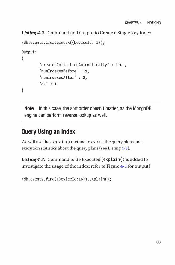
83
Listing 4-2. Command and Output to Create a Single Key Index
>db.events.createIndex({DeviceId: 1});
Output:
{
"createdCollectionAutomatically" : true,
"numIndexesBefore" : 1,
"numIndexesAfter" : 2,
"ok" : 1
}
Note In this case, the sort order doesn’t matter, as the MongodB engine can perform reverse lookup as well.
Query Using an Index
We will use the explain() method to extract the query plans and
execution statistics about the query plans (see Listing 4-3).
Listing 4-3. Command to Be Executed (explain() is added to
investigate the usage of the index; refer to Figure 4-1 for output)
>db.events.find({DeviceId:16}).explain();
Chapter 4 IndexIng
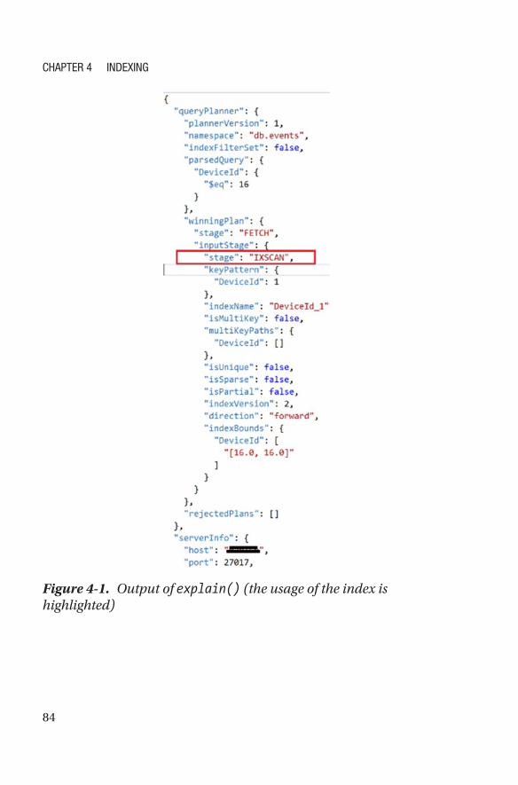
84
Figure 4-1. Output of explain() (the usage of the index is highlighted)
Chapter 4 IndexIng
85
In the explain() method, under winningPlan ➤ inputStage ➤ stage,
are the following five possible operations:
1. COLLSCAN: This represents the query that is to
perform the collection scan.
2. IXSCAN: This represents the usage of the index
(scanning index keys).
3. FETCH: This represents the operation retrieving the
documents.
4. SHARD_MERGE: This represents the merging of results
from the shards.
5. SHARDING_FILTER: This filters out the orphan
documents from shards.
As you can see in Figure 4-1, the winningPlan ➤ stage using IXSCAN
shows that the query is using indexes.
Query Not Using an Index
Now, let’s consider an example in which the field we have selected is not
using an index. See Listing 4-4 for details.
Listing 4-4. Execution of find with explain() and Its Output
> db.events.find( { "SensorId": 9 }).explain();
Output:
{
"queryPlanner": {
"plannerVersion": 1,
"namespace": "db.events",
"indexFilterSet": false,
"parsedQuery": {
Chapter 4 IndexIng
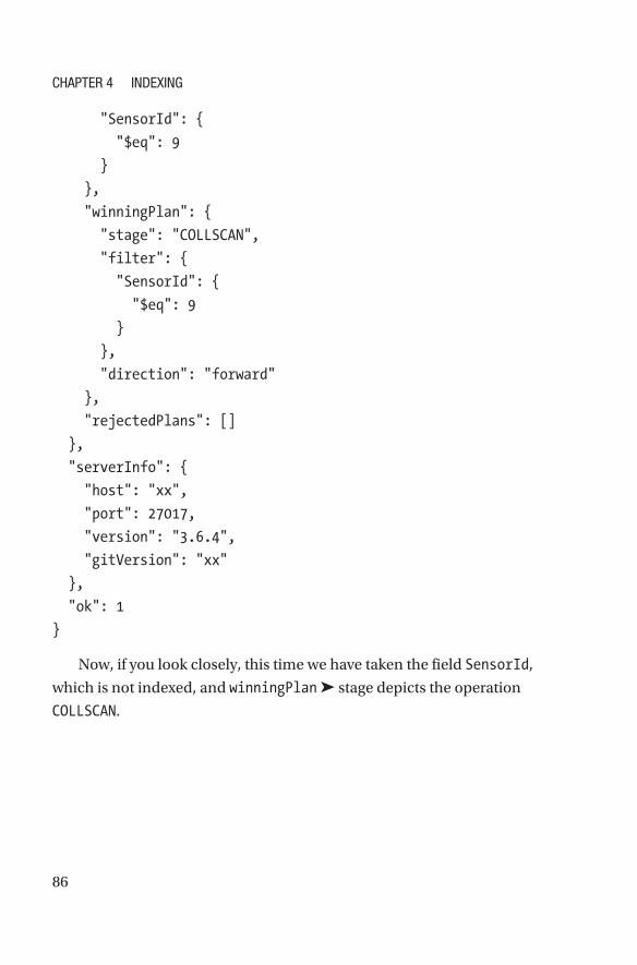
86
"SensorId": {
"$eq": 9
}
},
"winningPlan": {
"stage": "COLLSCAN",
"filter": {
"SensorId": {
"$eq": 9
}
},
"direction": "forward"
},
"rejectedPlans": []
},
"serverInfo": {
"host": "xx",
"port": 27017,
"version": "3.6.4",
"gitVersion": "xx"
},
"ok": 1
}
Now, if you look closely, this time we have taken the field SensorId,
which is not indexed, and winningPlan ➤ stage depicts the operation
COLLSCAN.
Chapter 4 IndexIng
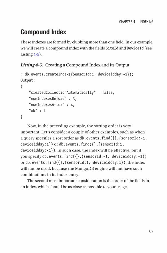
87
Compound IndexThese indexes are formed by clubbing more than one field. In our example,
we will create a compound index with the fields SiteId and DeviceId (see
Listing 4-5).
Listing 4-5. Creating a Compound Index and Its Output
> db.events.createIndex({SensorId:1, deviceidday:-1});
Output:
{
"createdCollectionAutomatically" : false,
"numIndexesBefore" : 3,
"numIndexesAfter" : 4,
"ok" : 1
}
Now, in the preceding example, the sorting order is very
important. Let’s consider a couple of other examples, such as when
a query specifies a sort order as db.events.find({},{sensorId:-1,
deviceidday:1}) or db.events.find({},{sensorId:1,
deviceidday:-1}). In such case, the index will be effective, but if
you specify db.events.find({},{sensorId:-1, deviceidday:-1})
or db.events.find({},{sensorId:1, deviceidday:1}), the index
will not be used, because the MongoDB engine will not have such
combinations in its index entry.
The second most important consideration is the order of the fields in
an index, which should be as close as possible to your usage.
Chapter 4 IndexIng
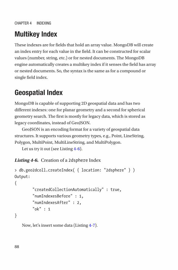
88
Multikey IndexThese indexes are for fields that hold an array value. MongoDB will create
an index entry for each value in the field. It can be constructed for scalar
values (number, string, etc.) or for nested documents. The MongoDB
engine automatically creates a multikey index if it senses the field has array
or nested documents. So, the syntax is the same as for a compound or
single field index.
Geospatial IndexMongoDB is capable of supporting 2D geospatial data and has two
different indexes: one for planar geometry and a second for spherical
geometry search. The first is mostly for legacy data, which is stored as
legacy coordinates, instead of GeoJSON.
GeoJSON is an encoding format for a variety of geospatial data
structures. It supports various geometry types, e.g., Point, LineString,
Polygon, MultiPoint, MultiLineString, and MultiPolygon.
Let us try it out (see Listing 4-6).
Listing 4-6. Creation of a 2dsphere Index
> db.geo2dcoll.createIndex( { location: "2dsphere" } )
Output:
{
"createdCollectionAutomatically" : true,
"numIndexesBefore" : 1,
"numIndexesAfter" : 2,
"ok" : 1
}
Now, let’s insert some data (Listing 4-7).
Chapter 4 IndexIng

89
Listing 4-7. Inserting Some Coordinates in the 2dsphere Index
> db.geo2dcoll.insertOne({location: {type: "Point",
coordinates: [28.354153, 77.373746]}});
> db.geo2dcoll.insertOne({location: {type: "Point",
coordinates: [28.370091, 77.315462]}});
To find the nearest point within 6.5 kilometers, refer to Listing 4-8.
Listing 4-8. Search for Nearest Point
>db.geo2dcoll.find({ location: { $near: { $geometry:
{ type: "Point", coordinates: [
28.354153, 77.373746 ] }, $maxDistance:
6500, $minDistance: 300 } } });
Output:
{ "_id" : ObjectId("5afdc37f83ae6a55a8f185ba"), "location" : {
"type" : "Point", "coordinates" : [ 28.370091, 77.315462 ] } }
Let’s now try using the 2D index. Refer to Listing 4-9 to create the index.
Listing 4-9. Creation of a 2D Index
> db.geo2dcoll1.createIndex( { location: "2d" } )
{
"createdCollectionAutomatically" : true,
"numIndexesBefore" : 1,
"numIndexesAfter" : 2,
"ok" : 1
}
Insert some locations (Listing 4-10).
Chapter 4 IndexIng
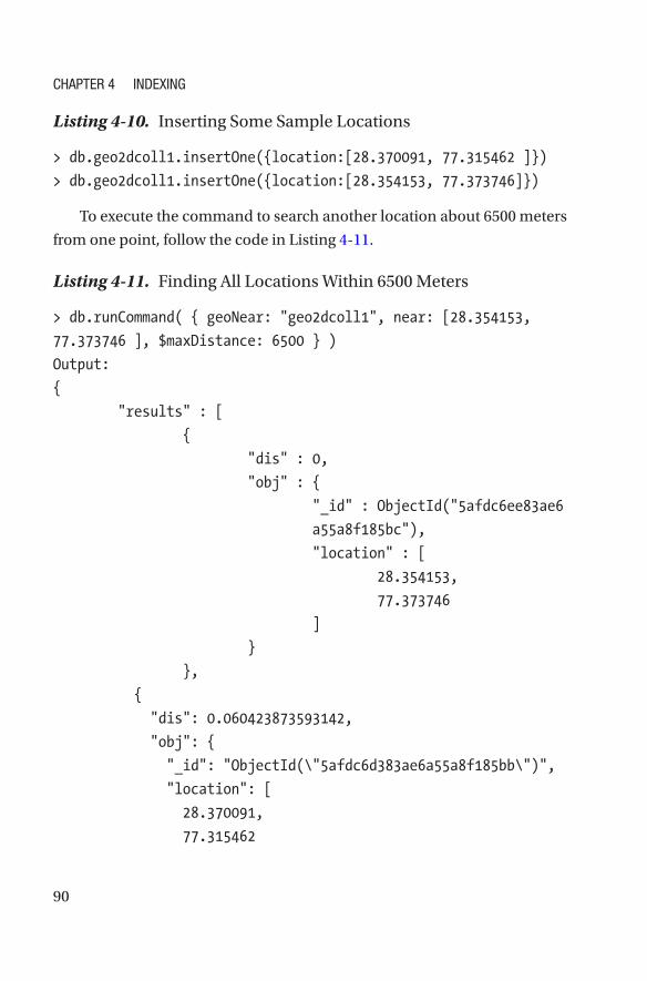
90
Listing 4-10. Inserting Some Sample Locations
> db.geo2dcoll1.insertOne({location:[28.370091, 77.315462 ]})
> db.geo2dcoll1.insertOne({location:[28.354153, 77.373746]})
To execute the command to search another location about 6500 meters
from one point, follow the code in Listing 4-11.
Listing 4-11. Finding All Locations Within 6500 Meters
> db.runCommand( { geoNear: "geo2dcoll1", near: [28.354153,
77.373746 ], $maxDistance: 6500 } )
Output:
{
"results" : [
{
"dis" : 0,
"obj" : {
"_id" : ObjectId("5afdc6ee83ae6
a55a8f185bc"),
"location" : [
28.354153,
77.373746
]
}
},
{
"dis": 0.060423873593142,
"obj": {
"_id": "ObjectId(\"5afdc6d383ae6a55a8f185bb\")",
"location": [
28.370091,
77.315462
Chapter 4 IndexIng
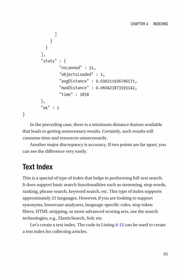
91
]
}
}
],
"stats" : {
"nscanned" : 31,
"objectsLoaded" : 2,
"avgDistance" : 0.030211936796571,
"maxDistance" : 0.060423873593142,
"time" : 1858
},
"ok" : 1
}
In the preceding case, there is a minimum distance feature available
that leads to getting unnecessary results. Certainly, such results will
consume time and resources unnecessarily.
Another major discrepancy is accuracy. If two points are far apart, you
can see the difference very easily.
Text IndexThis is a special of type of index that helps in performing full-text search.
It does support basic search functionalities such as stemming, stop words,
ranking, phrase search, keyword search, etc. This type of index supports
approximately 21 languages. However, if you are looking to support
synonyms, lowercase analyzers, language-specific rules, stop token
filters, HTML stripping, or more advanced scoring sets, use the search
technologies, e.g., ElasticSearch, Solr, etc.
Let’s create a text index. The code in Listing 4-12 can be used to create
a text index for collecting articles.
Chapter 4 IndexIng
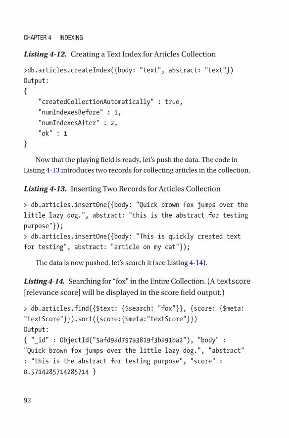
92
Listing 4-12. Creating a Text Index for Articles Collection
>db.articles.createIndex({body: "text", abstract: "text"})
Output:
{
"createdCollectionAutomatically" : true,
"numIndexesBefore" : 1,
"numIndexesAfter" : 2,
"ok" : 1
}
Now that the playing field is ready, let’s push the data. The code in
Listing 4-13 introduces two records for collecting articles in the collection.
Listing 4-13. Inserting Two Records for Articles Collection
> db.articles.insertOne({body: "Quick brown fox jumps over the
little lazy dog.", abstract: "this is the abstract for testing
purpose"});
> db.articles.insertOne({body: "This is quickly created text
for testing", abstract: "article on my cat"});
The data is now pushed, let’s search it (see Listing 4-14).
Listing 4-14. Searching for “fox” in the Entire Collection. (A textscore
[relevance score] will be displayed in the score field output.)
> db.articles.find({$text: {$search: "fox"}}, {score: {$meta:
"textScore"}}).sort({score:{$meta:"textScore"}})
Output:
{ "_id" : ObjectId("5afd9ad797a3819f3ba91ba2"), "body" :
"Quick brown fox jumps over the little lazy dog.", "abstract"
: "this is the abstract for testing purpose", "score" :
0.5714285714285714 }
Chapter 4 IndexIng

93
Hashed IndexThis type of index is used for sharding a database that uses a hashing
function to hash the value of the field, to distribute data across shards.
The most important thing to keep in mind in hashed indexes is that they
don’t support multikey indexes, and an application is not required to
know about the hash function, as the MongoDB database engine does the
necessary conversions automatically.
Use the code in Listing 4-15 to create a hashed index.
Listing 4-15. Creating a Hashed Index
> db.articles.createIndex( { _id: "hashed" } )
Output:
{
"createdCollectionAutomatically" : false,
"numIndexesBefore" : 2,
"numIndexesAfter" : 3,
"ok" : 1
}
Indexing in Azure Cosmos DBHaving so many types of indexes and then selecting and managing them
can be a headache. What if we could offload all our worries? There is
an answer. It is none other than Azure Cosmos DB. It will solve all your
indexing worries by automatically indexing everything (by default, the
indexing is enabled on all fields), whatever you push, so it will help to
reduce the cost per read. It has special indexes for spatial data, unique
indexing capabilities that you can define selectively, arrays, nested
documents, and, most important, it does sharding automatically. (See
Chapter 5 for further details.) This makes Azure Cosmos DB a completely
schema-free NoSQL database engine.
Chapter 4 IndexIng
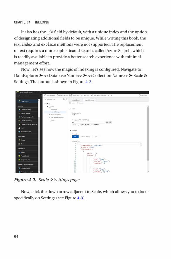
94
Now, click the down arrow adjacent to Scale, which allows you to focus
specifically on Settings (see Figure 4-3).
It also has the _id field by default, with a unique index and the option
of designating additional fields to be unique. While writing this book, the
text index and explain methods were not supported. The replacement
of text requires a more sophisticated search, called Azure Search, which
is readily available to provide a better search experience with minimal
management effort.
Now, let’s see how the magic of indexing is configured. Navigate to
DataExplorer ➤ <<Database Name>> ➤ <<Collection Name>> ➤ Scale &
Settings. The output is shown in Figure 4-2.
Figure 4-2. Scale & Settings page
Chapter 4 IndexIng
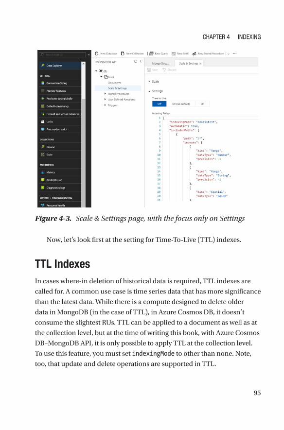
95
Figure 4-3. Scale & Settings page, with the focus only on Settings
Now, let’s look first at the setting for Time-To-Live (TTL) indexes.
TTL IndexesIn cases where-in deletion of historical data is required, TTL indexes are
called for. A common use case is time series data that has more significance
than the latest data. While there is a compute designed to delete older
data in MongoDB (in the case of TTL), in Azure Cosmos DB, it doesn’t
consume the slightest RUs. TTL can be applied to a document as well as at
the collection level, but at the time of writing this book, with Azure Cosmos
DB–MongoDB API, it is only possible to apply TTL at the collection level.
To use this feature, you must set indexingMode to other than none. Note,
too, that update and delete operations are supported in TTL.
Chapter 4 IndexIng
96
Now it’s time to use the same MongoDB shell for Cosmos DB. Open
the shell and execute the code in Listings 4-16 and 4-17.
Listing 4-16. Connecting Azure Cosmos DB Account from
MongoDB Shell
>sudo mongo <CosmosDBAccount>.documents.azure.
com:10255/<dbname> -u <CosmosDBAccount> -p <primary/secondary
key> --ssl --sslAllowInvalidCertificates
Listing 4-17. Create TTL Index Using the Shell Command
globaldb:PRIMARY> db.tscollection.createIndex( { "_ts": 1 }, {
expireAfterSeconds: 3600 } )
Output:
{
"createdCollectionAutomatically" : true,
"numIndexesBefore" : 1,
"numIndexesAfter" : 2,
"ok" : 1
}
Other indexes are supported by Azure Cosmos DB, which helps in
handling specific use cases. We’ll explore some of these in more detail in
the subsequent sections of this chapter.
Array IndexesThese types of indexes address query optimization for fields that consist of
array values. Each array value is indexed individually. In MongoDB, there
is no need for you to write a separate index for each array. If a field consists
of an array, it is included in an array index. For path strings, you must
specify the path of the array index, and it will index it like an array index.
Chapter 4 IndexIng
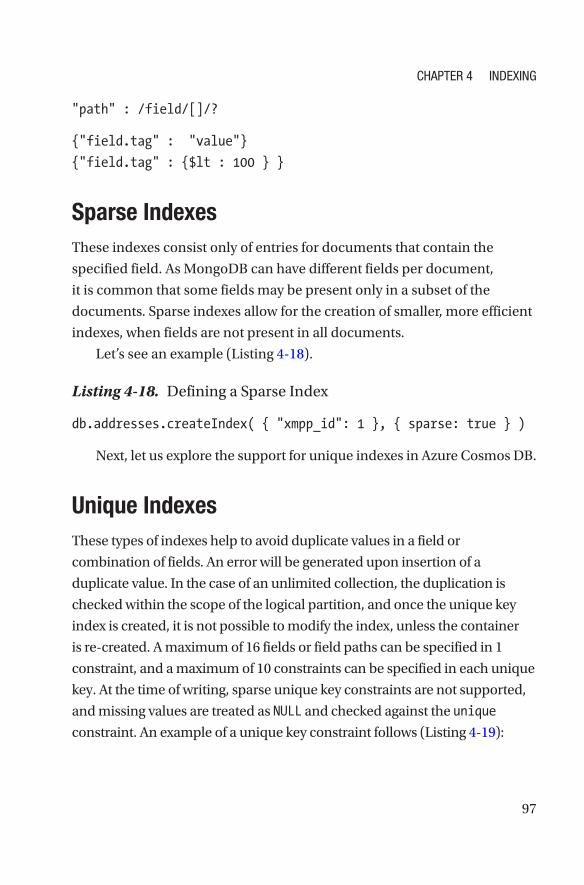
97
"path" : /field/[]/?
{"field.tag" : "value"}
{"field.tag" : {$lt : 100 } }
Sparse IndexesThese indexes consist only of entries for documents that contain the
specified field. As MongoDB can have different fields per document,
it is common that some fields may be present only in a subset of the
documents. Sparse indexes allow for the creation of smaller, more efficient
indexes, when fields are not present in all documents.
Let’s see an example (Listing 4-18).
Listing 4-18. Defining a Sparse Index
db.addresses.createIndex( { "xmpp_id": 1 }, { sparse: true } )
Next, let us explore the support for unique indexes in Azure Cosmos DB.
Unique IndexesThese types of indexes help to avoid duplicate values in a field or
combination of fields. An error will be generated upon insertion of a
duplicate value. In the case of an unlimited collection, the duplication is
checked within the scope of the logical partition, and once the unique key
index is created, it is not possible to modify the index, unless the container
is re-created. A maximum of 16 fields or field paths can be specified in 1
constraint, and a maximum of 10 constraints can be specified in each unique
key. At the time of writing, sparse unique key constraints are not supported,
and missing values are treated as NULL and checked against the unique
constraint. An example of a unique key constraint follows (Listing 4-19):
Chapter 4 IndexIng
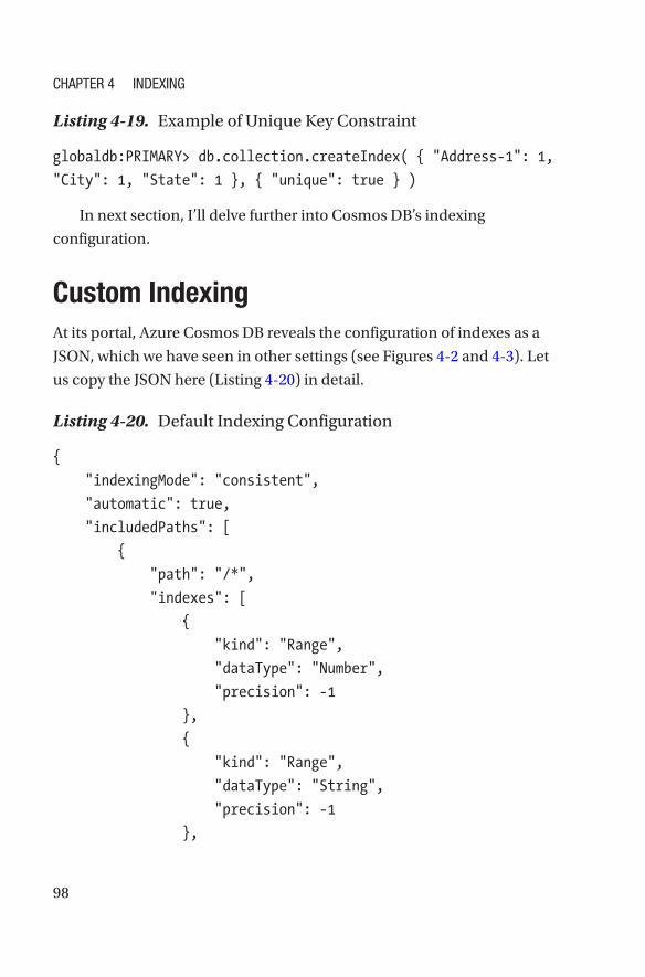
98
Listing 4-19. Example of Unique Key Constraint
globaldb:PRIMARY> db.collection.createIndex( { "Address-1": 1,
"City": 1, "State": 1 }, { "unique": true } )
In next section, I’ll delve further into Cosmos DB’s indexing
configuration.
Custom IndexingAt its portal, Azure Cosmos DB reveals the configuration of indexes as a
JSON, which we have seen in other settings (see Figures 4-2 and 4-3). Let
us copy the JSON here (Listing 4-20) in detail.
Listing 4-20. Default Indexing Configuration
{
"indexingMode": "consistent",
"automatic": true,
"includedPaths": [
{
"path": "/*",
"indexes": [
{
"kind": "Range",
"dataType": "Number",
"precision": -1
},
{
"kind": "Range",
"dataType": "String",
"precision": -1
},
Chapter 4 IndexIng
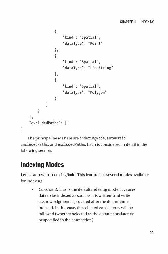
99
{
"kind": "Spatial",
"dataType": "Point"
},
{
"kind": "Spatial",
"dataType": "LineString"
},
{
"kind": "Spatial",
"dataType": "Polygon"
}
]
}
],
"excludedPaths": []
}
The principal heads here are indexingMode, automatic,
includedPaths, and excludedPaths. Each is considered in detail in the
following section.
Indexing ModesLet us start with indexingMode. This feature has several modes available
for indexing.
• Consistent: This is the default indexing mode. It causes
data to be indexed as soon as it is written, and write
acknowledgment is provided after the document is
indexed. In this case, the selected consistency will be
followed (whether selected as the default consistency
or specified in the connection).
Chapter 4 IndexIng
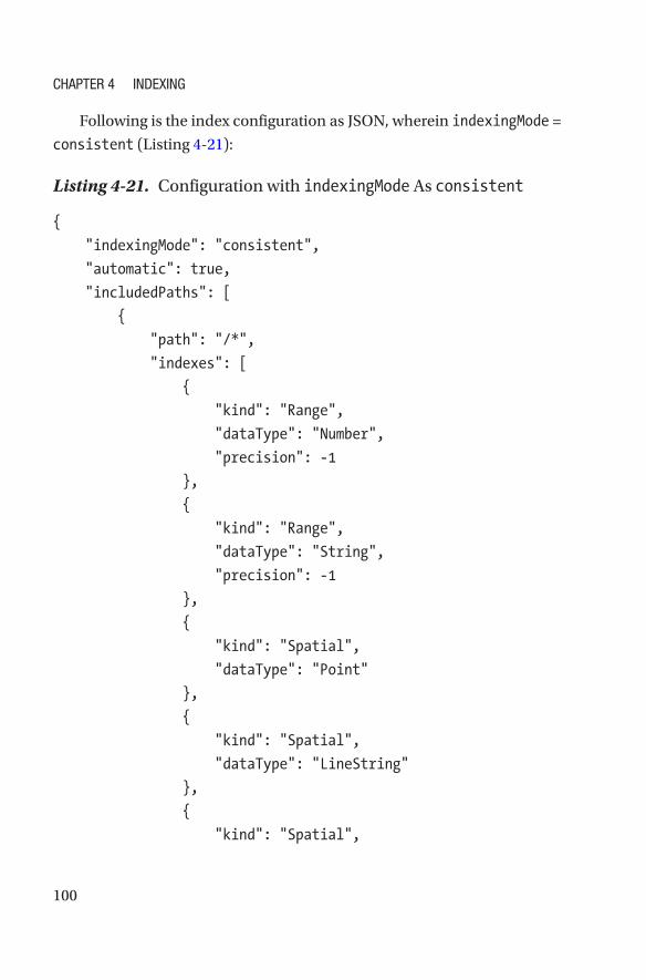
100
Following is the index configuration as JSON, wherein indexingMode =
consistent (Listing 4-21):
Listing 4-21. Configuration with indexingMode As consistent
{
"indexingMode": "consistent",
"automatic": true,
"includedPaths": [
{
"path": "/*",
"indexes": [
{
"kind": "Range",
"dataType": "Number",
"precision": -1
},
{
"kind": "Range",
"dataType": "String",
"precision": -1
},
{
"kind": "Spatial",
"dataType": "Point"
},
{
"kind": "Spatial",
"dataType": "LineString"
},
{
"kind": "Spatial",
Chapter 4 IndexIng
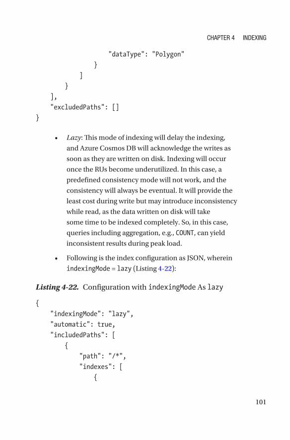
101
"dataType": "Polygon"
}
]
}
],
"excludedPaths": []
}
• Lazy: This mode of indexing will delay the indexing,
and Azure Cosmos DB will acknowledge the writes as
soon as they are written on disk. Indexing will occur
once the RUs become underutilized. In this case, a
predefined consistency mode will not work, and the
consistency will always be eventual. It will provide the
least cost during write but may introduce inconsistency
while read, as the data written on disk will take
some time to be indexed completely. So, in this case,
queries including aggregation, e.g., COUNT, can yield
inconsistent results during peak load.
• Following is the index configuration as JSON, wherein
indexingMode = lazy (Listing 4-22):
Listing 4-22. Configuration with indexingMode As lazy
{
"indexingMode": "lazy",
"automatic": true,
"includedPaths": [
{
"path": "/*",
"indexes": [
{
Chapter 4 IndexIng
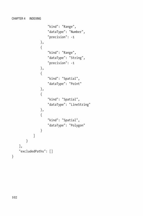
102
"kind": "Range",
"dataType": "Number",
"precision": -1
},
{
"kind": "Range",
"dataType": "String",
"precision": -1
},
{
"kind": "Spatial",
"dataType": "Point"
},
{
"kind": "Spatial",
"dataType": "LineString"
},
{
"kind": "Spatial",
"dataType": "Polygon"
}
]
}
],
"excludedPaths": []
}
Chapter 4 IndexIng
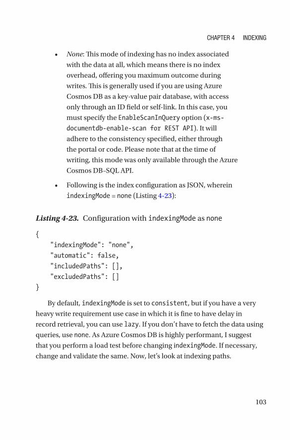
103
• None: This mode of indexing has no index associated
with the data at all, which means there is no index
overhead, offering you maximum outcome during
writes. This is generally used if you are using Azure
Cosmos DB as a key-value pair database, with access
only through an ID field or self-link. In this case, you
must specify the EnableScanInQuery option (x-ms-
documentdb-enable-scan for REST API). It will
adhere to the consistency specified, either through
the portal or code. Please note that at the time of
writing, this mode was only available through the Azure
Cosmos DB–SQL API.
• Following is the index configuration as JSON, wherein
indexingMode = none (Listing 4-23):
Listing 4-23. Configuration with indexingMode as none
{
"indexingMode": "none",
"automatic": false,
"includedPaths": [],
"excludedPaths": []
}
By default, indexingMode is set to consistent, but if you have a very
heavy write requirement use case in which it is fine to have delay in
record retrieval, you can use lazy. If you don’t have to fetch the data using
queries, use none. As Azure Cosmos DB is highly performant, I suggest
that you perform a load test before changing indexingMode. If necessary,
change and validate the same. Now, let’s look at indexing paths.
Chapter 4 IndexIng
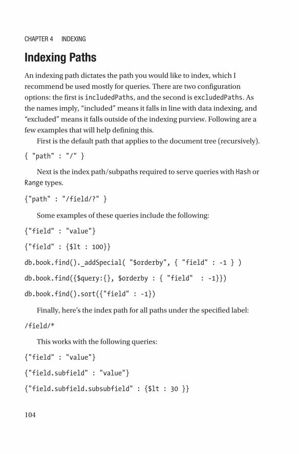
104
Indexing PathsAn indexing path dictates the path you would like to index, which I
recommend be used mostly for queries. There are two configuration
options: the first is includedPaths, and the second is excludedPaths. As
the names imply, “included” means it falls in line with data indexing, and
“excluded” means it falls outside of the indexing purview. Following are a
few examples that will help defining this.
First is the default path that applies to the document tree (recursively).
{ "path" : "/" }
Next is the index path/subpaths required to serve queries with Hash or
Range types.
{"path" : "/field/?" }
Some examples of these queries include the following:
{"field" : "value"}
{"field" : {$lt : 100}}
db.book.find()._addSpecial( "$orderby", { "field" : -1 } )
db.book.find({$query:{}, $orderby : { "field" : -1}})
db.book.find().sort({"field" : -1})
Finally, here’s the index path for all paths under the specified label:
/field/*
This works with the following queries:
{"field" : "value"}
{"field.subfield" : "value"}
{"field.subfield.subsubfield" : {$lt : 30 }}
Chapter 4 IndexIng
105
Index KindsAs with MongoDB, Azure Cosmos DB includes the following indexes:
Hash Indexes
Azure Cosmos DB performs hash-based indexing, which supports equality
queries and join queries efficiently. A built-in Hash function performs
mapping of hash values with the index key. By default, for all the string
data types, hash indexes are used.
Following is an example (Listing 4-24):
Listing 4-24. Sample Query That Uses a Hash Index
globaldb:PRIMARY> db.book.find({TestStatus : "Pass"});
Range Indexes
For range queries having operations (e.g., $lt, $gt,$ lte, $gte, $ne) or sort
order or equality, a range index will be used. It is a default index type for all
non-string and spatial data types.
Following are sample queries using a range key index (Listing 4-25):
Listing 4-25. Sample Queries Using a Range Index
globaldb:PRIMARY> db.book.find({DeviceId : {"$gt":1}});
globaldb:PRIMARY> db.book.find({DeviceId : {"$gt":1}},{},
{_SiteId:-1});
Geospatial Indexes
These types of indexes help to optimize queries related to location within
a two-dimensional space, such as projection systems for the earth.
Example of such queries would be those that contain a polygon or points
that are closest to a given point or line; those within a circle, rectangle,
Chapter 4 IndexIng
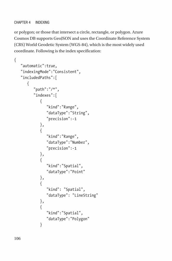
106
or polygon; or those that intersect a circle, rectangle, or polygon. Azure
Cosmos DB supports GeoJSON and uses the Coordinate Reference System
(CRS) World Geodetic System (WGS-84), which is the most widely used
coordinate. Following is the index specification:
{ "automatic":true, "indexingMode":"Consistent", "includedPaths":[ { "path":"/*", "indexes":[ { "kind":"Range", "dataType":"String", "precision":-1 }, { "kind":"Range", "dataType":"Number", "precision":-1 }, { "kind":"Spatial", "dataType":"Point" }, { "kind": "Spatial", "dataType": "LineString" }, { "kind":"Spatial", "dataType":"Polygon" }
Chapter 4 IndexIng

107
] } ], "excludedPaths":[ ]
}
Currently, the data type support available for spatial indexes includes
Point, Polygon, or LineString. Following are some examples you can use
(Listing 4-26):
Listing 4-26. Inserting Some Coordinates
> db.geo2dcoll.insertOne({location: {type: "Point",
coordinates: [28.354153, 77.373746]}});
> db.geo2dcoll.insertOne({location: {type: "Point",
coordinates: [28.370091, 77.315462]}});
Now, find the nearest point within 6.5 kilometers, using the code in
Listing 4-27.
Listing 4-27. Searching for the Nearest Point
>db.geo2dcoll.
find({ location: { $near: { $geometry:
{ type: "Point" , coordinates: [ 28.354153,
77.373746 ] }, $maxDistance:
6500, $minDistance: 300 } } });
Output:
{ "_id" : ObjectId("5afdc37f83ae6a55a8f185ba"), "location" : {
"type" : "Point", "coordinates" : [ 28.370091, 77.315462 ] } }
Chapter 4 IndexIng
108
Index PrecisionThis is important for balancing index storage vs. query performance. Better
precision means higher storage. However, this is practical only for string
data types. As for numbers, JSON consists of a minimum of 8 bytes, and
using 1–7 will reduce the precision and inhibit the reduction of storage
overhead. Spatial changing precision is not allowed. In string, this is useful,
because the length of a string can be arbitrary, and, by default, the scope
is full. However, if there is any use case that doesn’t require the entire
text to be indexed, you can configure it as 1–100 and -1 (maximum). No
equivalent exists in MongoDB.
Data TypesData types in index paths support String, Number, Point, Polygon, or
LineString. (One of these can be specified in one path.)
ConclusionBy default in Azure Cosmos DB, all data will be indexed automatically with
the optimal configuration, which provides flexibility in making schematic
changes and helps to achieve maximum performance. Also, it doesn’t limit
users only to automatic indexing. Instead, it provides greater flexibility of
customization.
Chapter 4 IndexIng
109© Manish Sharma 2018 M. Sharma, Cosmos DB for MongoDB Developers, https://doi.org/10.1007/978-1-4842-3682-6_5
CHAPTER 5
PartitioningScale, scale, scale…For most of the professional life span of a database
architect, these words reverberate whenever a new application is being
developed. The most difficult challenge is to design a database in
elastic mode. In the world of relational database management systems
(RDBMSs), this can occasionally be a nightmare, and it is a difficult task
in realm of NoSQL too. In this chapter, you are going to learn how, using
partitioning, Azure Cosmos DB scales databases.
ShardingIn MongoDB, scaling is handled through a process called sharding. This is
a manual configuration process that helps in scaling a MongoDB instance,
by adding more compute and storage. MongoDB executes the sharding of
data at a collection level; therefore, each collection is spread to multiple
shards, refer Figure 5-1.
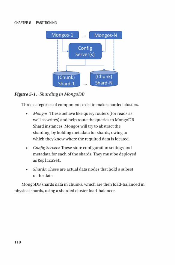
110
Three categories of components exist to make sharded clusters.
• Mongos: These behave like query routers (for reads as
well as writes) and help route the queries to MongoDB
Shard instances. Mongos will try to abstract the
sharding, by holding metadata for shards, owing to
which they know where the required data is located.
• Config Servers: These store configuration settings and
metadata for each of the shards. They must be deployed
as ReplicaSet.
• Shards: These are actual data nodes that hold a subset
of the data.
MongoDB shards data in chunks, which are then load-balanced in
physical shards, using a sharded cluster load-balancer.
Figure 5-1. Sharding in MongoDB
Chapter 5 partitioning
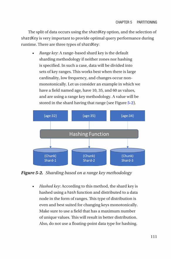
111
The split of data occurs using the shardKey option, and the selection of
shardKey is very important to provide optimal query performance during
runtime. There are three types of shardKey:
• Range key: A range-based shard key is the default
sharding methodology if neither zones nor hashing
is specified. In such a case, data will be divided into
sets of key ranges. This works best when there is large
cardinality, low frequency, and changes occur non-
monotonically. Let us consider an example in which we
have a field named age, have 10, 35, and 60 as values,
and are using a range key methodology. A value will be
stored in the shard having that range (see Figure 5-2).
• Hashed key: According to this method, the shard key is
hashed using a hash function and distributed to a data
node in the form of ranges. This type of distribution is
even and best suited for changing keys monotonically.
Make sure to use a field that has a maximum number
of unique values. This will result in better distribution.
Also, do not use a floating-point data type for hashing.
Figure 5-2. Sharding based on a range key methodology
Chapter 5 partitioning
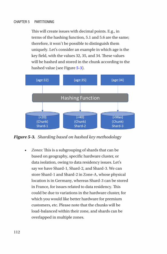
112
This will create issues with decimal points. E.g., in
terms of the hashing function, 5.1 and 5.6 are the same;
therefore, it won’t be possible to distinguish them
uniquely. Let’s consider an example in which age is the
key field, with the values 32, 35, and 34. These values
will be hashed and stored in the chunk according to the
hashed value (see Figure 5-3).
• Zones: This is a subgrouping of shards that can be
based on geography, specific hardware cluster, or
data isolation, owing to data residency issues. Let’s
say we have Shard-1, Shard-2, and Shard-3. We can
store Shard-1 and Shard-2 in Zone-A, whose physical
location is in Germany, whereas Shard-3 can be stored
in France, for issues related to data residency. This
could be due to variations in the hardware cluster, for
which you would like better hardware for premium
customers, etc. Please note that the chunks will be
load-balanced within their zone, and shards can be
overlapped in multiple zones.
Figure 5-3. Sharding based on hashed key methodology
Chapter 5 partitioning
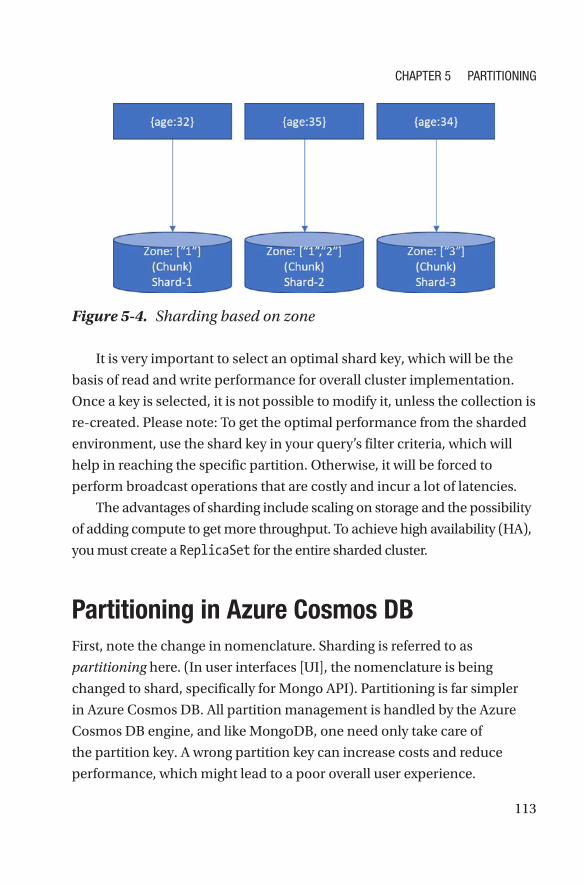
113
It is very important to select an optimal shard key, which will be the
basis of read and write performance for overall cluster implementation.
Once a key is selected, it is not possible to modify it, unless the collection is
re-created. Please note: To get the optimal performance from the sharded
environment, use the shard key in your query’s filter criteria, which will
help in reaching the specific partition. Otherwise, it will be forced to
perform broadcast operations that are costly and incur a lot of latencies.
The advantages of sharding include scaling on storage and the possibility
of adding compute to get more throughput. To achieve high availability (HA),
you must create a ReplicaSet for the entire sharded cluster.
Partitioning in Azure Cosmos DBFirst, note the change in nomenclature. Sharding is referred to as
partitioning here. (In user interfaces [UI], the nomenclature is being
changed to shard, specifically for Mongo API). Partitioning is far simpler
in Azure Cosmos DB. All partition management is handled by the Azure
Cosmos DB engine, and like MongoDB, one need only take care of
the partition key. A wrong partition key can increase costs and reduce
performance, which might lead to a poor overall user experience.
Figure 5-4. Sharding based on zone
Chapter 5 partitioning
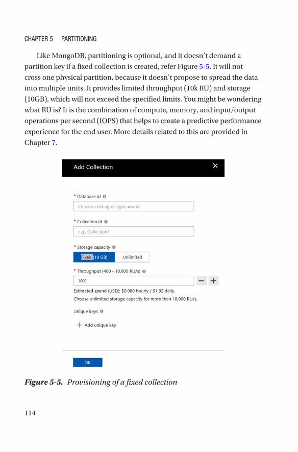
114
Figure 5-5. Provisioning of a fixed collection
Like MongoDB, partitioning is optional, and it doesn’t demand a
partition key if a fixed collection is created, refer Figure 5-5. It will not
cross one physical partition, because it doesn’t propose to spread the data
into multiple units. It provides limited throughput (10k RU) and storage
(10GB), which will not exceed the specified limits. You might be wondering
what RU is? It is the combination of compute, memory, and input/output
operations per second (IOPS) that helps to create a predictive performance
experience for the end user. More details related to this are provided in
Chapter 7.
Chapter 5 partitioning
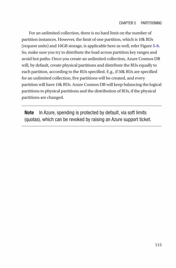
115
For an unlimited collection, there is no hard limit on the number of
partition instances. However, the limit of one partition, which is 10k RUs
(request units) and 10GB storage, is applicable here as well, refer Figure 5-6.
So, make sure you try to distribute the load across partition key ranges and
avoid hot paths. Once you create an unlimited collection, Azure Cosmos DB
will, by default, create physical partitions and distribute the RUs equally to
each partition, according to the RUs specified. E.g., if 50k RUs are specified
for an unlimited collection, five partitions will be created, and every
partition will have 10k RUs. Azure Cosmos DB will keep balancing the logical
partitions to physical partitions and the distribution of RUs, if the physical
partitions are changed.
Note in azure, spending is protected by default, via soft limits (quotas), which can be revoked by raising an azure support ticket.
Chapter 5 partitioning
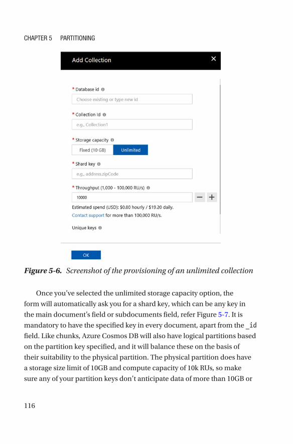
116
Figure 5-6. Screenshot of the provisioning of an unlimited collection
Once you’ve selected the unlimited storage capacity option, the
form will automatically ask you for a shard key, which can be any key in
the main document’s field or subdocuments field, refer Figure 5-7. It is
mandatory to have the specified key in every document, apart from the _id
field. Like chunks, Azure Cosmos DB will also have logical partitions based
on the partition key specified, and it will balance these on the basis of
their suitability to the physical partition. The physical partition does have
a storage size limit of 10GB and compute capacity of 10k RUs, so make
sure any of your partition keys don’t anticipate data of more than 10GB or
Chapter 5 partitioning
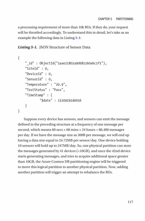
117
a processing requirement of more than 10k RUs. If they do, your request
will be throttled accordingly. To understand this in detail, let’s take as an
example the following data in Listing 5-1:
Listing 5-1. JSON Structure of Sensor Data
{
"_id" : ObjectId("5aae21802a90b85160a6c1f1"),
"SiteId" : 0,
"DeviceId" : 0,
"SensorId" : 0,
"Temperature" : "20.9",
"TestStatus" : "Pass",
"TimeStamp" : {
"$date" : 1520929246056
}
}
Suppose every device has sensors, and sensors can emit the message
defined in the preceding structure at a frequency of one message per
second, which means 60 secs × 60 mins × 24 hours = 86,400 messages
per day. If we have the message size as 300B per message, we will end up
having a data size equal to 24.72MB per sensor/day. One device holding
10 sensors will hold up to 247MB/day. So, one physical partition can store
the messages generated by 41 devices (<10GB), and once the 42nd device
starts generating messages, and tries to acquire additional space greater
than 10GB, the Azure Cosmos DB partitioning engine will be triggered
to move this logical partition to another physical partition. Now, adding
another partition will trigger an attempt to rebalance the RUs.
Chapter 5 partitioning
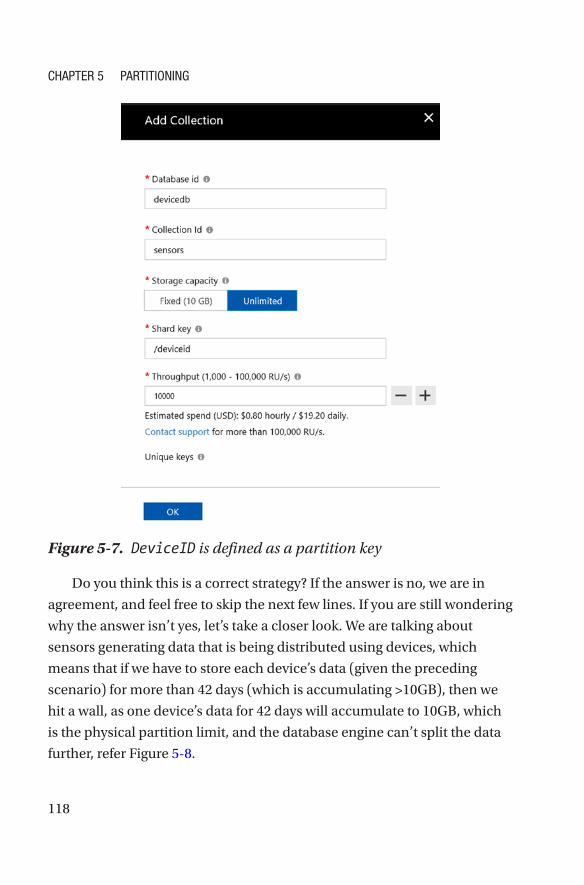
118
Do you think this is a correct strategy? If the answer is no, we are in
agreement, and feel free to skip the next few lines. If you are still wondering
why the answer isn’t yes, let’s take a closer look. We are talking about
sensors generating data that is being distributed using devices, which
means that if we have to store each device’s data (given the preceding
scenario) for more than 42 days (which is accumulating >10GB), then we
hit a wall, as one device’s data for 42 days will accumulate to 10GB, which
is the physical partition limit, and the database engine can’t split the data
further, refer Figure 5-8.
Figure 5-7. DeviceID is defined as a partition key
Chapter 5 partitioning
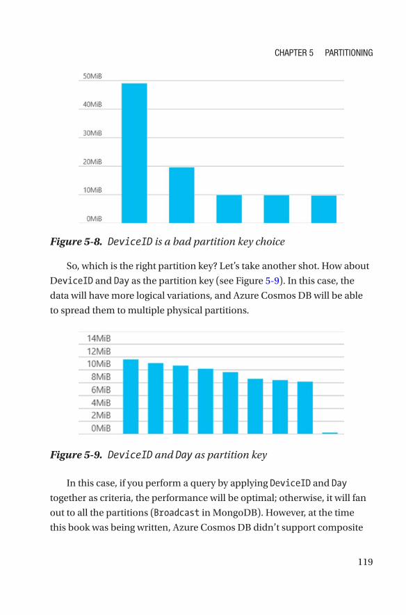
119
Figure 5-9. DeviceID and Day as partition key
So, which is the right partition key? Let’s take another shot. How about
DeviceID and Day as the partition key (see Figure 5-9). In this case, the
data will have more logical variations, and Azure Cosmos DB will be able
to spread them to multiple physical partitions.
Figure 5-8. DeviceID is a bad partition key choice
In this case, if you perform a query by applying DeviceID and Day
together as criteria, the performance will be optimal; otherwise, it will fan
out to all the partitions (Broadcast in MongoDB). However, at the time
this book was being written, Azure Cosmos DB didn’t support composite
Chapter 5 partitioning
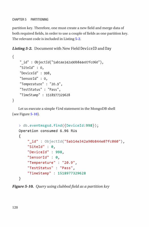
120
partition key. Therefore, one must create a new field and merge data of
both required fields, in order to use a couple of fields as one partition key.
The relevant code is included in Listing 5-2.
Listing 5-2. Document with New Field DeviceID and Day
{
"_id" : ObjectId("5ab14e342a90b844e07fc060"),
"SiteId" : 0,
"DeviceId" : 998,
"SensorId" : 0,
"Temperature" : "20.9",
"TestStatus" : "Pass",
"TimeStamp" : 1518977329628
}
Let us execute a simple find statement in the MongoDB shell
(see Figure 5-10).
Figure 5-10. Query using clubbed field as a partition key
Chapter 5 partitioning
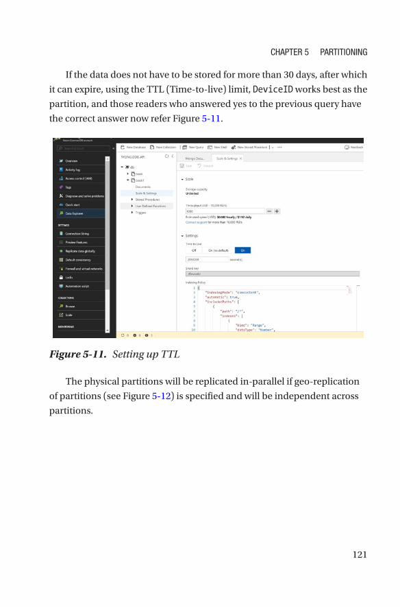
121
If the data does not have to be stored for more than 30 days, after which
it can expire, using the TTL (Time-to-live) limit, DeviceID works best as the
partition, and those readers who answered yes to the previous query have
the correct answer now refer Figure 5-11.
Figure 5-11. Setting up TTL
The physical partitions will be replicated in-parallel if geo-replication
of partitions (see Figure 5-12) is specified and will be independent across
partitions.
Chapter 5 partitioning
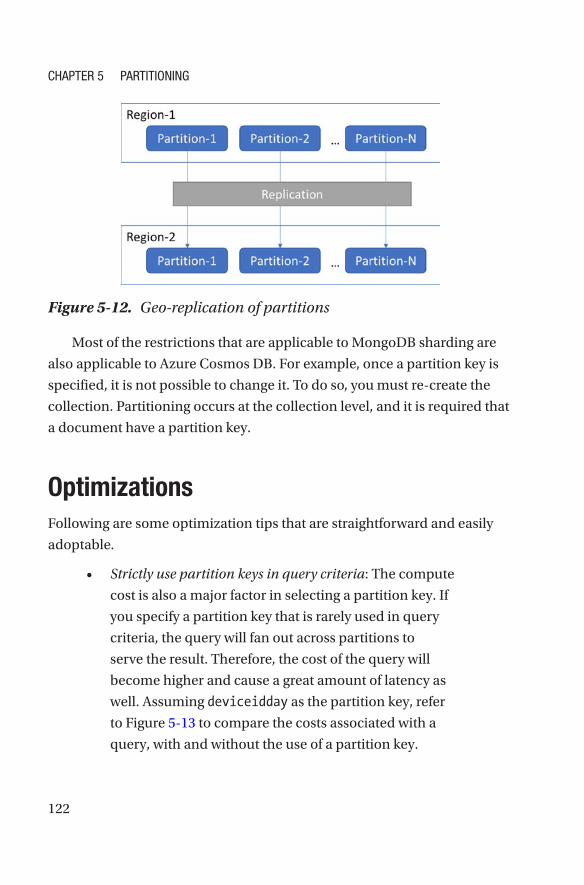
122
Most of the restrictions that are applicable to MongoDB sharding are
also applicable to Azure Cosmos DB. For example, once a partition key is
specified, it is not possible to change it. To do so, you must re-create the
collection. Partitioning occurs at the collection level, and it is required that
a document have a partition key.
OptimizationsFollowing are some optimization tips that are straightforward and easily
adoptable.
• Strictly use partition keys in query criteria: The compute
cost is also a major factor in selecting a partition key. If
you specify a partition key that is rarely used in query
criteria, the query will fan out across partitions to
serve the result. Therefore, the cost of the query will
become higher and cause a great amount of latency as
well. Assuming deviceidday as the partition key, refer
to Figure 5-13 to compare the costs associated with a
query, with and without the use of a partition key.
Figure 5-12. Geo-replication of partitions
Chapter 5 partitioning
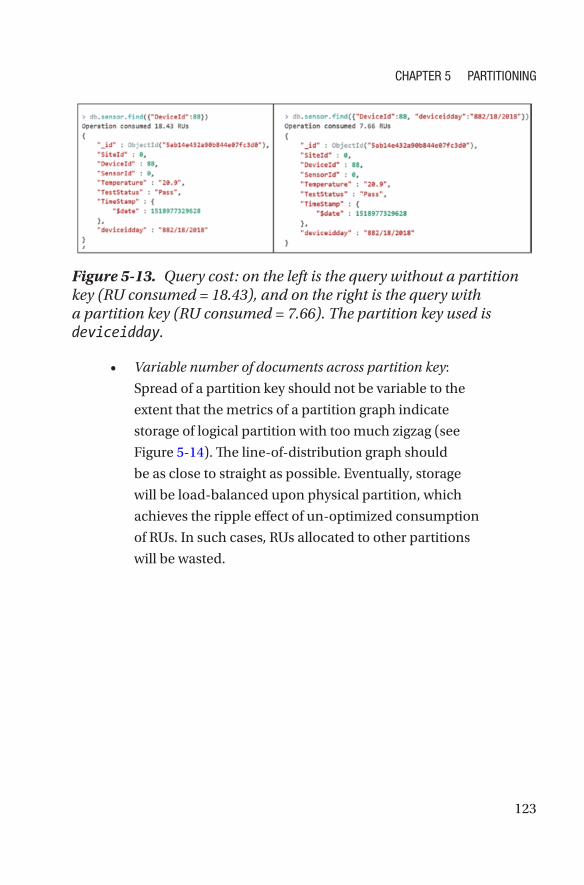
123
• Variable number of documents across partition key:
Spread of a partition key should not be variable to the
extent that the metrics of a partition graph indicate
storage of logical partition with too much zigzag (see
Figure 5-14). The line-of-distribution graph should
be as close to straight as possible. Eventually, storage
will be load-balanced upon physical partition, which
achieves the ripple effect of un-optimized consumption
of RUs. In such cases, RUs allocated to other partitions
will be wasted.
Figure 5-13. Query cost: on the left is the query without a partition key (RU consumed = 18.43), and on the right is the query with a partition key (RU consumed = 7.66). The partition key used is deviceidday.
Chapter 5 partitioning
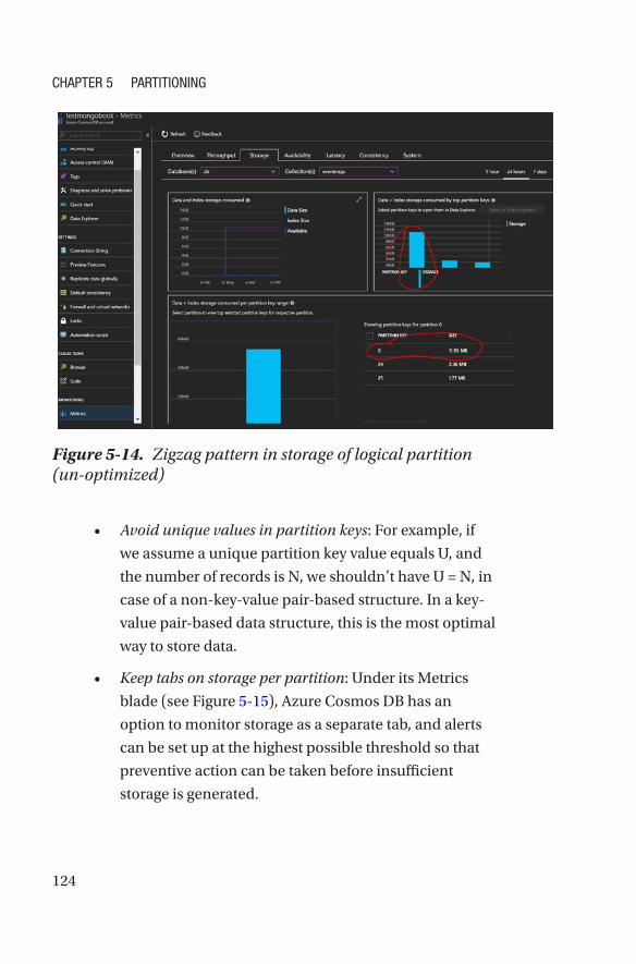
124
Figure 5-14. Zigzag pattern in storage of logical partition (un- optimized)
• Avoid unique values in partition keys: For example, if
we assume a unique partition key value equals U, and
the number of records is N, we shouldn’t have U = N, in
case of a non-key-value pair-based structure. In a key-
value pair-based data structure, this is the most optimal
way to store data.
• Keep tabs on storage per partition: Under its Metrics
blade (see Figure 5-15), Azure Cosmos DB has an
option to monitor storage as a separate tab, and alerts
can be set up at the highest possible threshold so that
preventive action can be taken before insufficient
storage is generated.
Chapter 5 partitioning
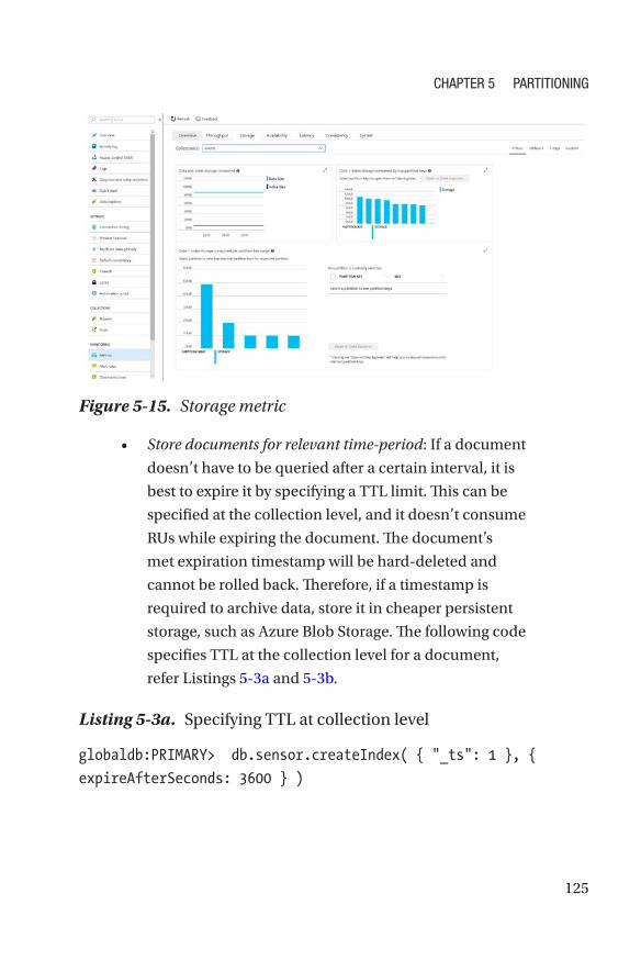
125
• Store documents for relevant time-period: If a document
doesn’t have to be queried after a certain interval, it is
best to expire it by specifying a TTL limit. This can be
specified at the collection level, and it doesn’t consume
RUs while expiring the document. The document’s
met expiration timestamp will be hard-deleted and
cannot be rolled back. Therefore, if a timestamp is
required to archive data, store it in cheaper persistent
storage, such as Azure Blob Storage. The following code
specifies TTL at the collection level for a document,
refer Listings 5-3a and 5-3b.
Listing 5-3a. Specifying TTL at collection level
globaldb:PRIMARY> db.sensor.createIndex( { "_ts": 1 }, {
expireAfterSeconds: 3600 } )
Figure 5-15. Storage metric
Chapter 5 partitioning
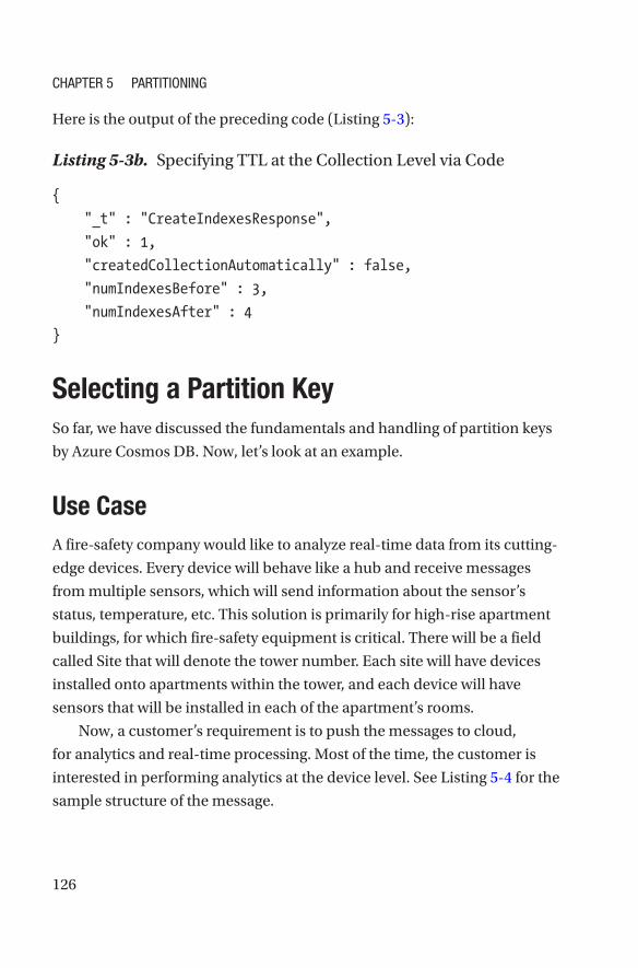
126
Here is the output of the preceding code (Listing 5-3):
Listing 5-3b. Specifying TTL at the Collection Level via Code
{
"_t" : "CreateIndexesResponse",
"ok" : 1,
"createdCollectionAutomatically" : false,
"numIndexesBefore" : 3,
"numIndexesAfter" : 4
}
Selecting a Partition KeySo far, we have discussed the fundamentals and handling of partition keys
by Azure Cosmos DB. Now, let’s look at an example.
Use CaseA fire-safety company would like to analyze real-time data from its cutting-
edge devices. Every device will behave like a hub and receive messages
from multiple sensors, which will send information about the sensor’s
status, temperature, etc. This solution is primarily for high-rise apartment
buildings, for which fire-safety equipment is critical. There will be a field
called Site that will denote the tower number. Each site will have devices
installed onto apartments within the tower, and each device will have
sensors that will be installed in each of the apartment’s rooms.
Now, a customer’s requirement is to push the messages to cloud,
for analytics and real-time processing. Most of the time, the customer is
interested in performing analytics at the device level. See Listing 5-4 for the
sample structure of the message.
Chapter 5 partitioning
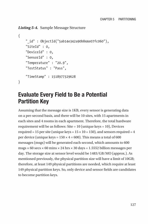
127
Listing 5-4. Sample Message Structure
{
"_id" : ObjectId("5ab14e342a90b844e07fc060"),
"SiteId" : 0,
"DeviceId" : 0,
"SensorId" : 0,
"Temperature" : "20.9",
"TestStatus" : "Pass",
"TimeStamp" : 1518977329628
}
Evaluate Every Field to Be a Potential Partition KeyAssuming that the message size is 1KB, every sensor is generating data
on a per-second basis, and there will be 10 sites, with 15 apartments in
each sites and 4 rooms in each apartment. Therefore, the total hardware
requirement will be as follows: Site = 10 (unique keys = 10), Devices
required = 15 per site (unique keys = 15 × 10 = 150), and sensors required = 4
per device (unique keys = 150 × 4 = 600). This means a total of 600
messages (msgs) will be generated each second, which amounts to 600
msgs × 60 secs × 60 mins × 24 hrs × 30 days = 1.5552 billion messages per
day. The storage size at sensor level would be 1483/GB/MO (approx.). As
mentioned previously, the physical partition size will have a limit of 10GB;
therefore, at least 149 physical partitions are needed, which require at least
149 physical partition keys. So, only device and sensor fields are candidates
to become partition keys.
Chapter 5 partitioning
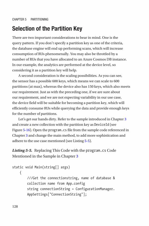
128
Selection of the Partition KeyThere are two important considerations to bear in mind. One is the
query pattern. If you don’t specify a partition key as one of the criteria,
the database engine will end up performing scans, which will increase
consumption of RUs phenomenally. You may also be throttled by a
number of RUs that you have allocated to an Azure Cosmos DB instance.
In our example, the analytics are performed at the device level, so
considering it as a partition key will help.
A second consideration is the scaling possibilities. As you can see,
the sensor has a possible 600 keys, which means we can scale to 600
partitions (at max), whereas the device also has 150 keys, which also meets
our requirement. Just as with the preceding one, if we are sure about
our requirement, and we are not expecting variability in our use case,
the device field will be suitable for becoming a partition key, which will
efficiently consume RUs while querying the data and provide enough keys
for the number of partitions.
Let’s get our hands dirty. Refer to the sample introduced in Chapter 3
and create a new collection with the partition key as DeviceId (see
Figure 5-16). Open the program.cs file from the sample code referenced in
Chapter 3 and change the main method, to add more sophistication and
adhere to the use case mentioned (see Listing 5-5).
Listing 5-5. Replacing This Code with the program.cs Code
Mentioned in the Sample in Chapter 3
static void Main(string[] args)
{
///Get the connectionstring, name of database &
collection name from App.config
string connectionString = ConfigurationManager.
AppSettings["ConnectionString"];
Chapter 5 partitioning
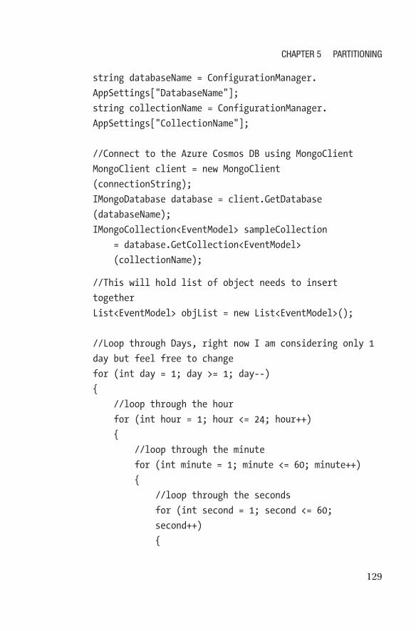
129
string databaseName = ConfigurationManager.
AppSettings["DatabaseName"];
string collectionName = ConfigurationManager.
AppSettings["CollectionName"];
//Connect to the Azure Cosmos DB using MongoClient
MongoClient client = new MongoClient
(connectionString);
IMongoDatabase database = client.GetDatabase
(databaseName);
IMongoCollection<EventModel> sampleCollection
= database.GetCollection<EventModel>
(collectionName);
//This will hold list of object needs to insert
together
List<EventModel> objList = new List<EventModel>();
//Loop through Days, right now I am considering only 1
day but feel free to change
for (int day = 1; day >= 1; day--)
{
//loop through the hour
for (int hour = 1; hour <= 24; hour++)
{
//loop through the minute
for (int minute = 1; minute <= 60; minute++)
{
//loop through the seconds
for (int second = 1; second <= 60;
second++)
{
Chapter 5 partitioning
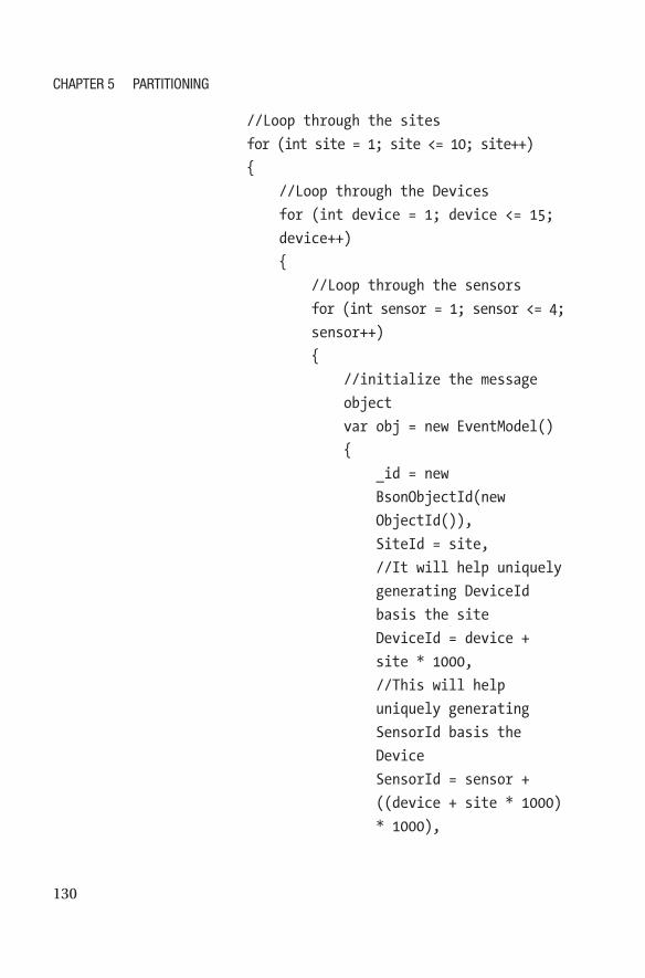
130
//Loop through the sites
for (int site = 1; site <= 10; site++)
{
//Loop through the Devices
for (int device = 1; device <= 15;
device++)
{
//Loop through the sensors
for (int sensor = 1; sensor <= 4;
sensor++)
{
//initialize the message
object
var obj = new EventModel()
{
_id = new
BsonObjectId(new
ObjectId()),
SiteId = site,
//It will help uniquely
generating DeviceId
basis the site
DeviceId = device +
site * 1000,
//This will help
uniquely generating
SensorId basis the
Device
SensorId = sensor +
((device + site * 1000)
* 1000),
Chapter 5 partitioning
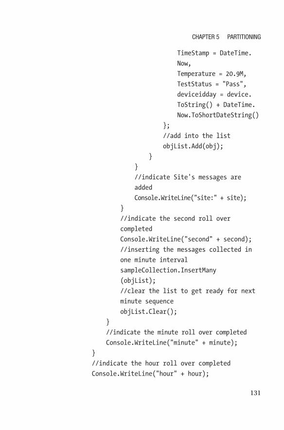
131
TimeStamp = DateTime.
Now,
Temperature = 20.9M,
TestStatus = "Pass",
deviceidday = device.
ToString() + DateTime.
Now.ToShortDateString()
};
//add into the list
objList.Add(obj);
}
}
//indicate Site's messages are
added
Console.WriteLine("site:" + site);
}
//indicate the second roll over
completed
Console.WriteLine("second" + second);
//inserting the messages collected in
one minute interval
sampleCollection.InsertMany
(objList);
//clear the list to get ready for next
minute sequence
objList.Clear();
}
//indicate the minute roll over completed
Console.WriteLine("minute" + minute);
}
//indicate the hour roll over completed
Console.WriteLine("hour" + hour);
Chapter 5 partitioning
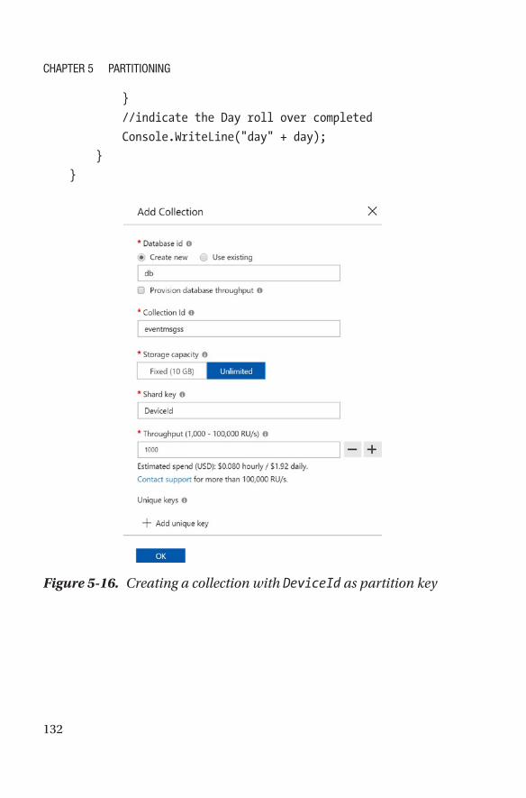
132
}
//indicate the Day roll over completed
Console.WriteLine("day" + day);
}
}
Figure 5-16. Creating a collection with DeviceId as partition key
Chapter 5 partitioning
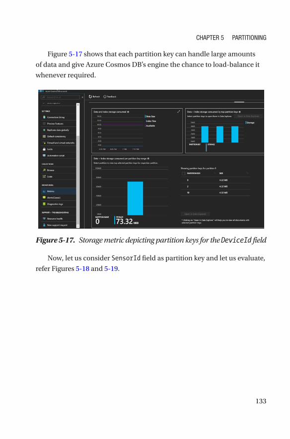
133
Figure 5-17 shows that each partition key can handle large amounts
of data and give Azure Cosmos DB’s engine the chance to load-balance it
whenever required.
Figure 5-17. Storage metric depicting partition keys for the DeviceId field
Now, let us consider SensorId field as partition key and let us evaluate,
refer Figures 5-18 and 5-19.
Chapter 5 partitioning
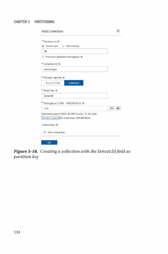
134
Figure 5-18. Creating a collection with the SensorId field as partition key
Chapter 5 partitioning
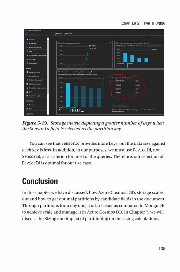
135
Figure 5-19. Storage metric depicting a greater number of keys when the SensorId field is selected as the partition key
You can see that SensorId provides more keys, but the data size against
each key is less. In addition, in our purposes, we must use DeviceId, not
SensorId, as a criterion for most of the queries. Therefore, our selection of
DeviceId is optimal for our use case.
ConclusionIn this chapter we have discussed, how Azure Cosmos DB’s storage scales
out and how to get optimal partitions by candidate fields in the document.
Through partitions from day one, it is far easier as compared to MongoDB
to achieve scale and manage it in Azure Cosmos DB. In Chapter 7, we will
discuss the Sizing and impact of partitioning on the sizing calculations.
Chapter 5 partitioning
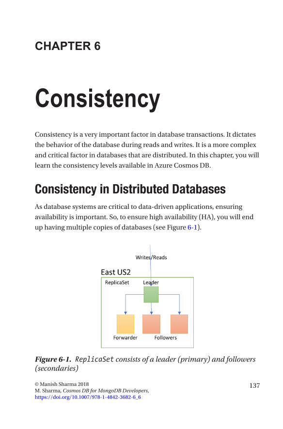
137© Manish Sharma 2018 M. Sharma, Cosmos DB for MongoDB Developers, https://doi.org/10.1007/978-1-4842-3682-6_6
CHAPTER 6
ConsistencyConsistency is a very important factor in database transactions. It dictates
the behavior of the database during reads and writes. It is a more complex
and critical factor in databases that are distributed. In this chapter, you will
learn the consistency levels available in Azure Cosmos DB.
Consistency in Distributed DatabasesAs database systems are critical to data-driven applications, ensuring
availability is important. So, to ensure high availability (HA), you will end
up having multiple copies of databases (see Figure 6-1).
Figure 6-1. ReplicaSet consists of a leader (primary) and followers (secondaries)
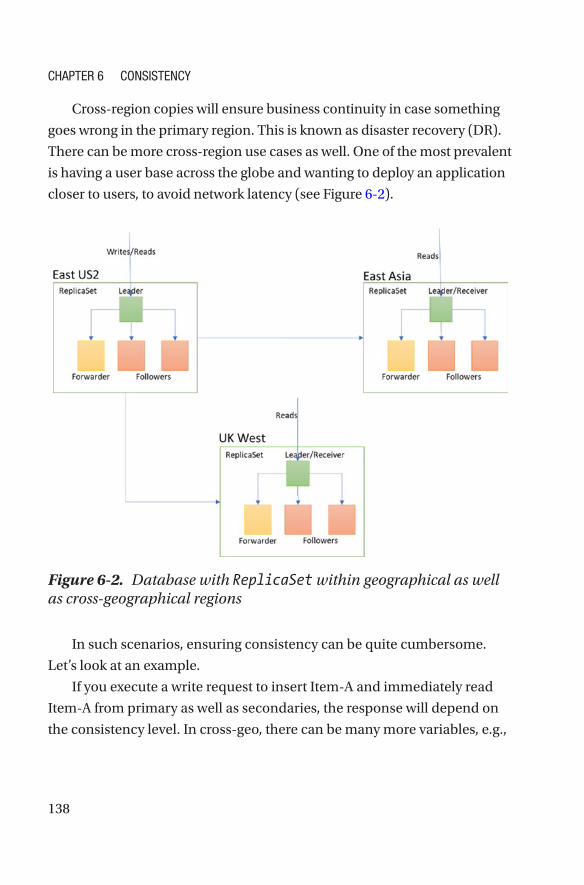
138
Cross-region copies will ensure business continuity in case something
goes wrong in the primary region. This is known as disaster recovery (DR).
There can be more cross-region use cases as well. One of the most prevalent
is having a user base across the globe and wanting to deploy an application
closer to users, to avoid network latency (see Figure 6-2).
In such scenarios, ensuring consistency can be quite cumbersome.
Let’s look at an example.
If you execute a write request to insert Item-A and immediately read
Item-A from primary as well as secondaries, the response will depend on
the consistency level. In cross-geo, there can be many more variables, e.g.,
Figure 6-2. Database with ReplicaSet within geographical as well as cross-geographical regions
Chapter 6 ConsistenCy
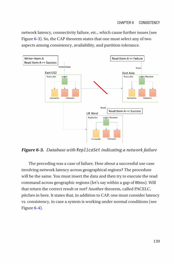
139
network latency, connectivity failure, etc., which cause further issues (see
Figure 6-3). So, the CAP theorem states that one must select any of two
aspects among consistency, availability, and partition tolerance.
The preceding was a case of failure. How about a successful use case
involving network latency across geographical regions? The procedure
will be the same. You must insert the data and then try to execute the read
command across geographic regions (let’s say within a gap of 80ms). Will
that return the correct result or not? Another theorem, called PACELC,
pitches in here. It states that, in addition to CAP, one must consider latency
vs. consistency, in case a system is working under normal conditions (see
Figure 6-4).
Figure 6-3. Database with ReplicaSet indicating a network failure
Chapter 6 ConsistenCy
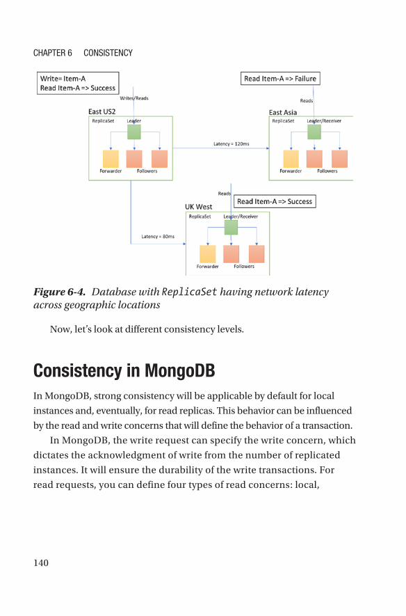
140
Now, let’s look at different consistency levels.
Consistency in MongoDBIn MongoDB, strong consistency will be applicable by default for local
instances and, eventually, for read replicas. This behavior can be influenced
by the read and write concerns that will define the behavior of a transaction.
In MongoDB, the write request can specify the write concern, which
dictates the acknowledgment of write from the number of replicated
instances. It will ensure the durability of the write transactions. For
read requests, you can define four types of read concerns: local,
Figure 6-4. Database with ReplicaSet having network latency across geographic locations
Chapter 6 ConsistenCy
141
available, majority, and linearizable. In the case of “local,” irrespective
of the write concern, data will be available from the primary instance,
without ensuring a durable commitment to other replicas. It defaults to
read concern against primary, and it defaults to secondary, if the reads
are associated with causally consistent sessions. For “available,” the
behavior remains the same as for “local,” except that it defaults to read
concern for secondaries when a causal consistent session is not there
and is not available when causal consistency is set. The “majority”
read concern will revert to more consistent data, after a majority of
nodes acknowledge the writes. The “linearizable” read will wait until
a majority of replicas acknowledge the writes, which ensures the most
consistent read of all the read concerns. This can be defined only for
primary instance/master node.
You can execute the command by explicitly specifying the read
concern in MongoDB (see Listing 6-1).
Listing 6-1. MongoDB’s Shell Command for Specifying Read Concern
db.collection.find().readConcern(<"majority"|"local"|"linearizable"|
"available">)
If you are working in a distributed database environment, ensuring
that you can read your writes is a challenge, as it will take some time to
replicate your writes. In practice, setting up a linearizable read concern is
often not possible, as it will increase latency. Recently, in MongoDB 3.6,
a client session was introduced in which the reads/writes are consistent
within the scope of the user session, which is called causal consistency. It
will ensure that you will not have performance glitches and still allow you
to be able to read your writes.
Chapter 6 ConsistenCy
142
Consistency in Azure Cosmos DBAzure Cosmos DB has five types of consistency: strong, bounded staleness,
session, consistent prefix, and eventual. To understand this completely, let
us define two groups of consistency behavior: consistent reads/writes and
high throughput.
Consistent Reads/WritesAzure Cosmos DB offers the possibility of consistent reads/writes with
three characteristics: strong consistency, bounded staleness, and session
staleness. To understand their behavior, let’s consider a few examples of
each.
Listing 6-2 gives the code for a sample document that we will be using
to explore various consistency levels.
Listing 6-2. Code for Sample Document
{ "_id" : "469", "SiteId" : 0, "DeviceId" : 0, "SensorId" : 0,
"Temperature" : "20.9", "TestStatus" : "Pass", "deviceidday" :
"03/10/2018" }
Strong Consistency
For strong consistency, Azure Cosmos DB ensures that writes are visible
only after they are committed as durable by both the primary and a
majority of replicas, or are aborted. A client can never see uncommitted
or partially committed writes and is guaranteed to read the latest
acknowledged write (see Figure 6-5).
Chapter 6 ConsistenCy
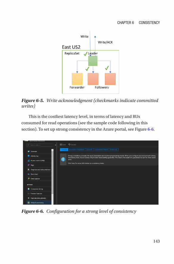
143
This is the costliest latency level, in terms of latency and RUs
consumed for read operations (see the sample code following in this
section). To set up strong consistency in the Azure portal, see Figure 6-6.
Figure 6-5. Write acknowledgment (checkmarks indicate committed writes)
Figure 6-6. Configuration for a strong level of consistency
Chapter 6 ConsistenCy
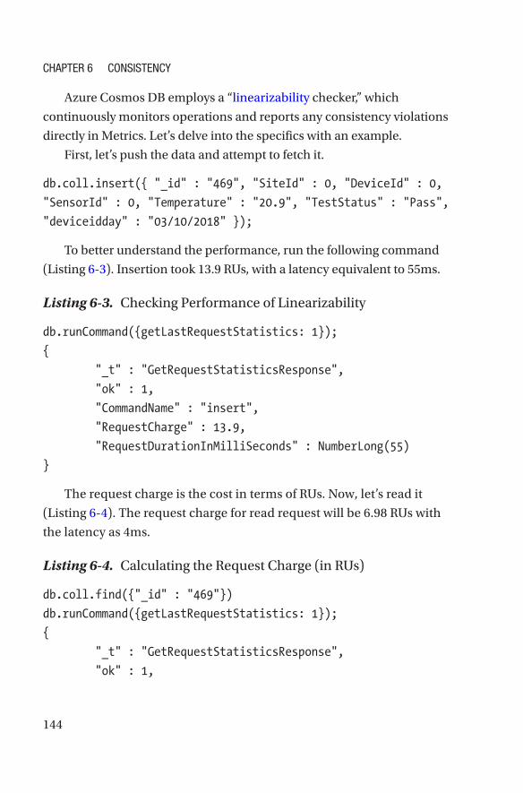
144
Azure Cosmos DB employs a “linearizability checker,” which
continuously monitors operations and reports any consistency violations
directly in Metrics. Let’s delve into the specifics with an example.
First, let’s push the data and attempt to fetch it.
db.coll.insert({ "_id" : "469", "SiteId" : 0, "DeviceId" : 0,
"SensorId" : 0, "Temperature" : "20.9", "TestStatus" : "Pass",
"deviceidday" : "03/10/2018" });
To better understand the performance, run the following command
(Listing 6-3). Insertion took 13.9 RUs, with a latency equivalent to 55ms.
Listing 6-3. Checking Performance of Linearizability
db.runCommand({getLastRequestStatistics: 1});
{
"_t" : "GetRequestStatisticsResponse",
"ok" : 1,
"CommandName" : "insert",
"RequestCharge" : 13.9,
"RequestDurationInMilliSeconds" : NumberLong(55)
}
The request charge is the cost in terms of RUs. Now, let’s read it
(Listing 6-4). The request charge for read request will be 6.98 RUs with
the latency as 4ms.
Listing 6-4. Calculating the Request Charge (in RUs)
db.coll.find({"_id" : "469"})
db.runCommand({getLastRequestStatistics: 1});
{
"_t" : "GetRequestStatisticsResponse",
"ok" : 1,
Chapter 6 ConsistenCy
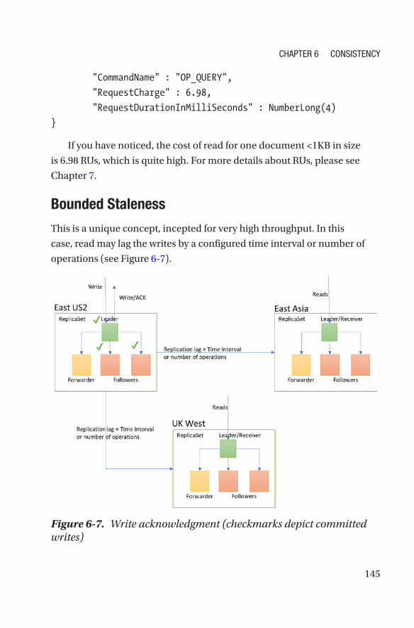
145
"CommandName" : "OP_QUERY",
"RequestCharge" : 6.98,
"RequestDurationInMilliSeconds" : NumberLong(4)
}
If you have noticed, the cost of read for one document <1KB in size
is 6.98 RUs, which is quite high. For more details about RUs, please see
Chapter 7.
Bounded Staleness
This is a unique concept, incepted for very high throughput. In this
case, read may lag the writes by a configured time interval or number of
operations (see Figure 6-7).
Figure 6-7. Write acknowledgment (checkmarks depict committed writes)
Chapter 6 ConsistenCy
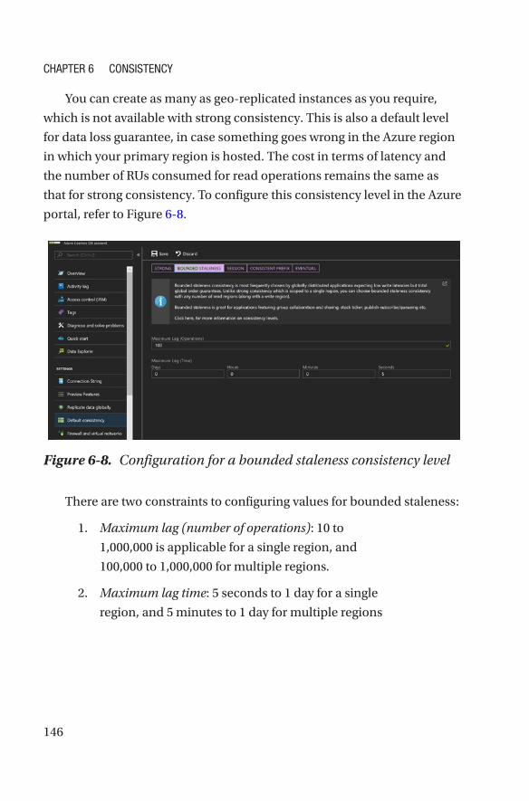
146
You can create as many as geo-replicated instances as you require,
which is not available with strong consistency. This is also a default level
for data loss guarantee, in case something goes wrong in the Azure region
in which your primary region is hosted. The cost in terms of latency and
the number of RUs consumed for read operations remains the same as
that for strong consistency. To configure this consistency level in the Azure
portal, refer to Figure 6-8.
There are two constraints to configuring values for bounded staleness:
1. Maximum lag (number of operations): 10 to
1,000,000 is applicable for a single region, and
100,000 to 1,000,000 for multiple regions.
2. Maximum lag time: 5 seconds to 1 day for a single
region, and 5 minutes to 1 day for multiple regions
Figure 6-8. Configuration for a bounded staleness consistency level
Chapter 6 ConsistenCy
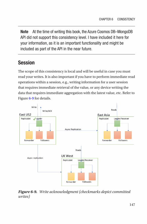
147
Note at the time of writing this book, the azure Cosmos DB–MongoDB api did not support this consistency level. i have included it here for your information, as it is an important functionality and might be included as part of the api in the near future.
Session
The scope of this consistency is local and will be useful in case you must
read your writes. It is also important if you have to perform immediate read
operations within a session, e.g., writing information for a user session
that requires immediate retrieval of the value, or any device writing the
data that requires immediate aggregation with the latest value, etc. Refer to
Figure 6-9 for details.
Figure 6-9. Write acknowledgment (checkmarks depict committed writes)
Chapter 6 ConsistenCy
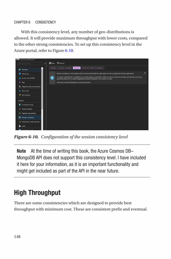
148
With this consistency level, any number of geo-distributions is
allowed. It will provide maximum throughput with lower costs, compared
to the other strong consistencies. To set up this consistency level in the
Azure portal, refer to Figure 6-10.
Note at the time of writing this book, the azure Cosmos DB–MongoDB api does not support this consistency level. i have included it here for your information, as it is an important functionality and might get included as part of the api in the near future.
High ThroughputThere are some consistencies which are designed to provide best
throughput with minimum cost. These are consistent prefix and eventual.
Figure 6-10. Configuration of the session consistency level
Chapter 6 ConsistenCy
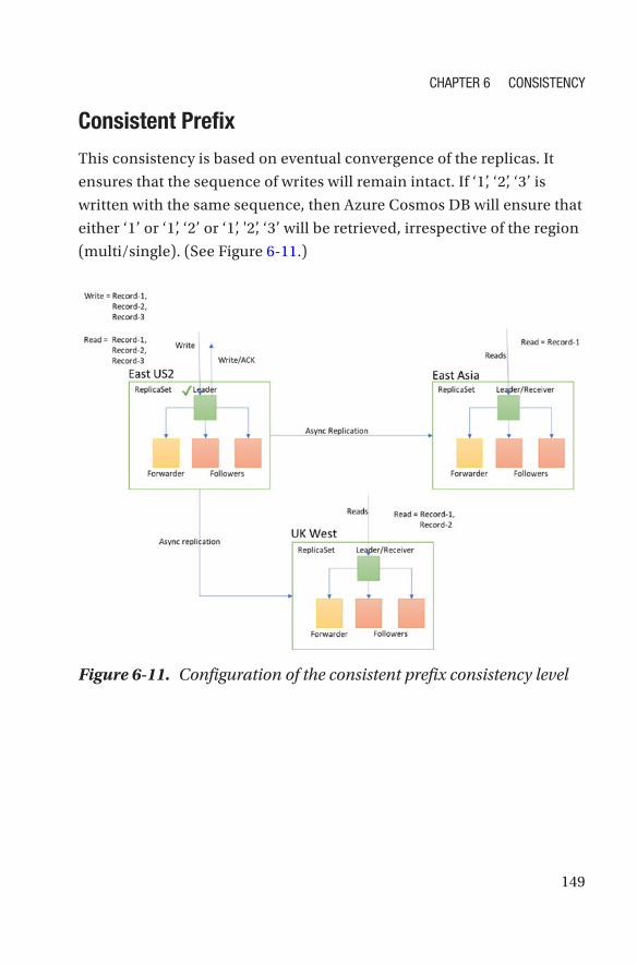
149
Consistent Prefix
This consistency is based on eventual convergence of the replicas. It
ensures that the sequence of writes will remain intact. If ‘1’, ‘2’, ‘3’ is
written with the same sequence, then Azure Cosmos DB will ensure that
either ‘1’ or ‘1’, ‘2’ or ‘1’, '2’, ‘3’ will be retrieved, irrespective of the region
(multi/single). (See Figure 6-11.)
Figure 6-11. Configuration of the consistent prefix consistency level
Chapter 6 ConsistenCy
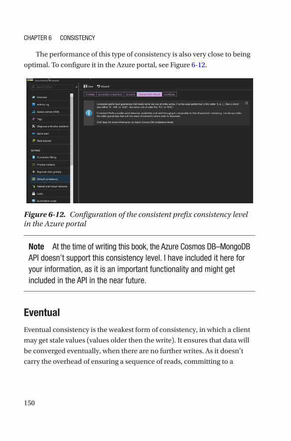
150
The performance of this type of consistency is also very close to being
optimal. To configure it in the Azure portal, see Figure 6-12.
Note at the time of writing this book, the azure Cosmos DB–MongoDB api doesn’t support this consistency level. i have included it here for your information, as it is an important functionality and might get included in the api in the near future.
Eventual
Eventual consistency is the weakest form of consistency, in which a client
may get stale values (values older then the write). It ensures that data will
be converged eventually, when there are no further writes. As it doesn’t
carry the overhead of ensuring a sequence of reads, committing to a
Figure 6-12. Configuration of the consistent prefix consistency level in the Azure portal
Chapter 6 ConsistenCy
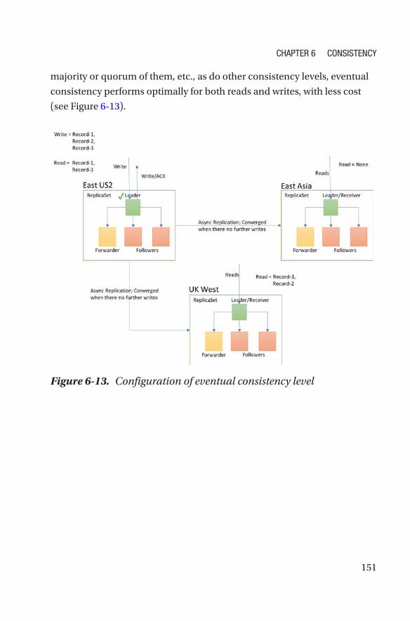
151
majority or quorum of them, etc., as do other consistency levels, eventual
consistency performs optimally for both reads and writes, with less cost
(see Figure 6-13).
Figure 6-13. Configuration of eventual consistency level
Chapter 6 ConsistenCy
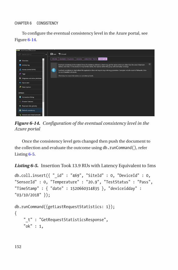
152
To configure the eventual consistency level in the Azure portal, see
Figure 6-14.
Once the consistency level gets changed then push the document to
the collection and evaluate the outcome using db.runCommand(), refer
Listing 6-5.
Listing 6-5. Insertion Took 13.9 RUs with Latency Equivalent to 5ms
db.coll.insert({ "_id" : "469", "SiteId" : 0, "DeviceId" : 0,
"SensorId" : 0, "Temperature" : "20.9", "TestStatus" : "Pass",
"TimeStamp" : { "date" : 1520660314835 }, "deviceidday" :
"03/10/2018" });
db.runCommand({getLastRequestStatistics: 1});
{
"_t" : "GetRequestStatisticsResponse",
"ok" : 1,
Figure 6-14. Configuration of the eventual consistency level in the Azure portal
Chapter 6 ConsistenCy
153
"CommandName" : "insert",
"RequestCharge" : 13.9,
"RequestDurationInMilliSeconds" : NumberLong(5)
}
Let us try to read the document (see Listing 6-6).
Listing 6-6. Request Charge for Read Request
db.coll.find({"_id" : "469"})
db.runCommand({getLastRequestStatistics: 1});
{
"_t" : "GetRequestStatisticsResponse",
"ok" : 1,
"CommandName" : "OP_QUERY",
"RequestCharge" : 3.49,
"RequestDurationInMilliSeconds" : NumberLong(4)
}
If you compare the request charge with that for strong consistency, it is
much less.
ConclusionI have discussed the various types of consistencies and explained that
some give comparable results, some are performant, and some assure
consistent reads. There is no rule of thumb governing the selection of one
over another, but it is suggested that you thoroughly analyze the use case
and select the appropriate consistency.
Chapter 6 ConsistenCy
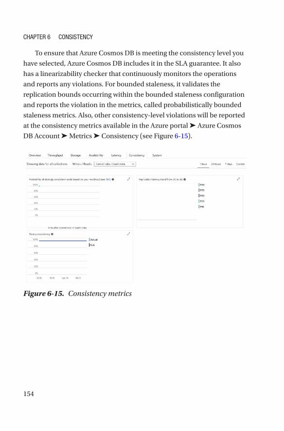
154
To ensure that Azure Cosmos DB is meeting the consistency level you
have selected, Azure Cosmos DB includes it in the SLA guarantee. It also
has a linearizability checker that continuously monitors the operations
and reports any violations. For bounded staleness, it validates the
replication bounds occurring within the bounded staleness configuration
and reports the violation in the metrics, called probabilistically bounded
staleness metrics. Also, other consistency-level violations will be reported
at the consistency metrics available in the Azure portal ➤ Azure Cosmos
DB Account ➤ Metrics ➤ Consistency (see Figure 6-15).
Figure 6-15. Consistency metrics
Chapter 6 ConsistenCy
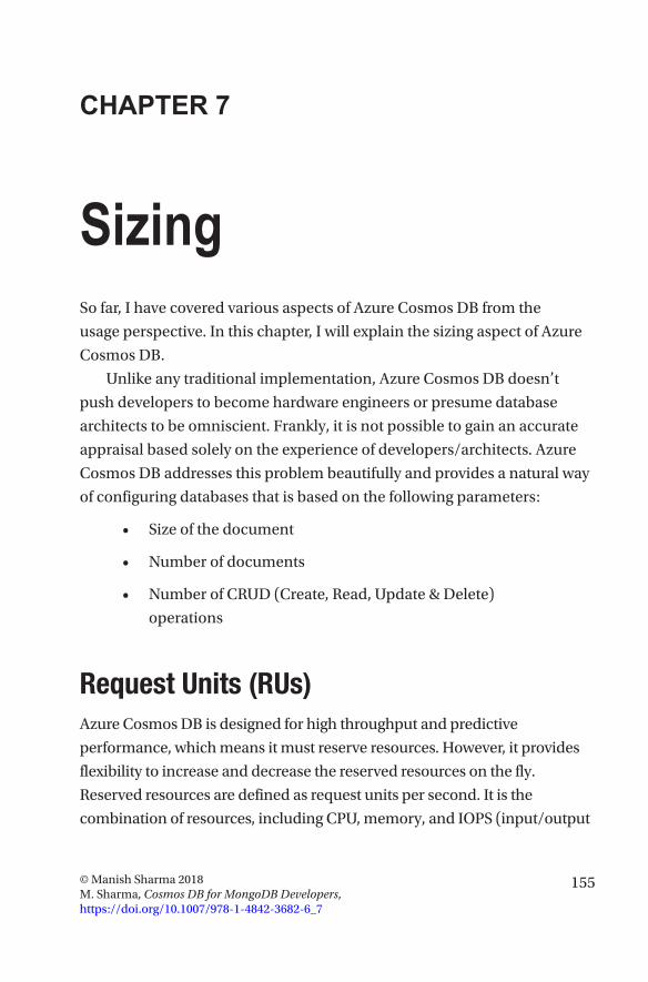
155© Manish Sharma 2018 M. Sharma, Cosmos DB for MongoDB Developers, https://doi.org/10.1007/978-1-4842-3682-6_7
CHAPTER 7
SizingSo far, I have covered various aspects of Azure Cosmos DB from the
usage perspective. In this chapter, I will explain the sizing aspect of Azure
Cosmos DB.
Unlike any traditional implementation, Azure Cosmos DB doesn’t
push developers to become hardware engineers or presume database
architects to be omniscient. Frankly, it is not possible to gain an accurate
appraisal based solely on the experience of developers/architects. Azure
Cosmos DB addresses this problem beautifully and provides a natural way
of configuring databases that is based on the following parameters:
• Size of the document
• Number of documents
• Number of CRUD (Create, Read, Update & Delete)
operations
Request Units (RUs)Azure Cosmos DB is designed for high throughput and predictive
performance, which means it must reserve resources. However, it provides
flexibility to increase and decrease the reserved resources on the fly.
Reserved resources are defined as request units per second. It is the
combination of resources, including CPU, memory, and IOPS (input/output
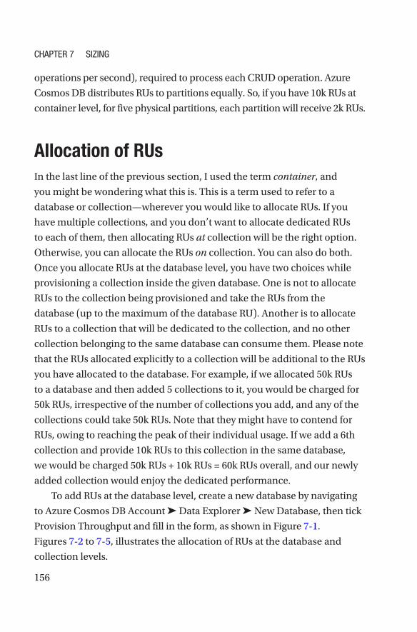
156
operations per second), required to process each CRUD operation. Azure
Cosmos DB distributes RUs to partitions equally. So, if you have 10k RUs at
container level, for five physical partitions, each partition will receive 2k RUs.
Allocation of RUsIn the last line of the previous section, I used the term container, and
you might be wondering what this is. This is a term used to refer to a
database or collection—wherever you would like to allocate RUs. If you
have multiple collections, and you don’t want to allocate dedicated RUs
to each of them, then allocating RUs at collection will be the right option.
Otherwise, you can allocate the RUs on collection. You can also do both.
Once you allocate RUs at the database level, you have two choices while
provisioning a collection inside the given database. One is not to allocate
RUs to the collection being provisioned and take the RUs from the
database (up to the maximum of the database RU). Another is to allocate
RUs to a collection that will be dedicated to the collection, and no other
collection belonging to the same database can consume them. Please note
that the RUs allocated explicitly to a collection will be additional to the RUs
you have allocated to the database. For example, if we allocated 50k RUs
to a database and then added 5 collections to it, you would be charged for
50k RUs, irrespective of the number of collections you add, and any of the
collections could take 50k RUs. Note that they might have to contend for
RUs, owing to reaching the peak of their individual usage. If we add a 6th
collection and provide 10k RUs to this collection in the same database,
we would be charged 50k RUs + 10k RUs = 60k RUs overall, and our newly
added collection would enjoy the dedicated performance.
To add RUs at the database level, create a new database by navigating
to Azure Cosmos DB Account ➤ Data Explorer ➤ New Database, then tick
Provision Throughput and fill in the form, as shown in Figure 7-1.
Figures 7-2 to 7-5, illustrates the allocation of RUs at the database and
collection levels.
Chapter 7 Sizing
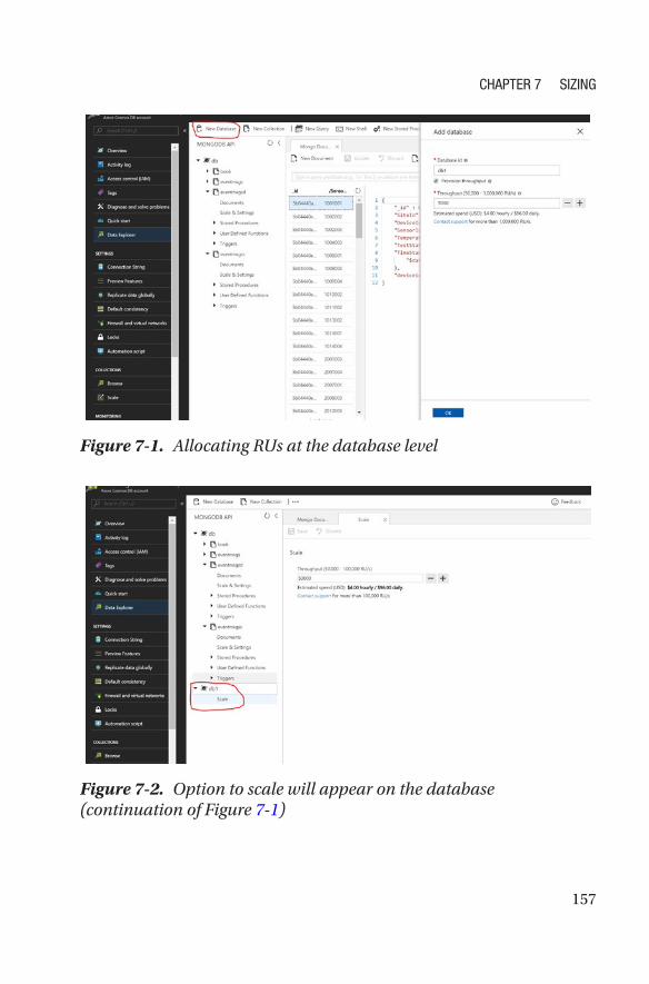
157
Figure 7-1. Allocating RUs at the database level
Figure 7-2. Option to scale will appear on the database (continuation of Figure 7-1)
Chapter 7 Sizing
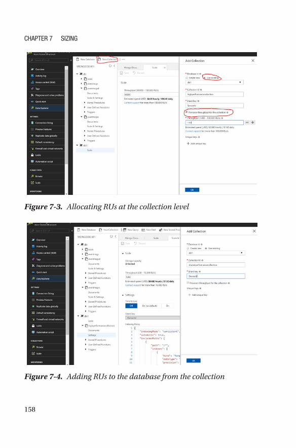
158
Figure 7-3. Allocating RUs at the collection level
Figure 7-4. Adding RUs to the database from the collection
Chapter 7 Sizing
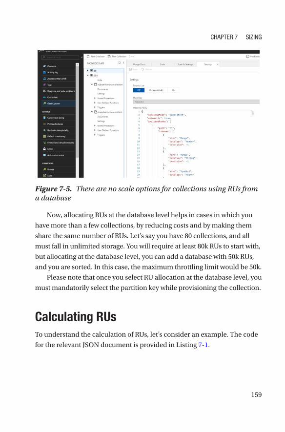
159
Now, allocating RUs at the database level helps in cases in which you
have more than a few collections, by reducing costs and by making them
share the same number of RUs. Let’s say you have 80 collections, and all
must fall in unlimited storage. You will require at least 80k RUs to start with,
but allocating at the database level, you can add a database with 50k RUs,
and you are sorted. In this case, the maximum throttling limit would be 50k.
Please note that once you select RU allocation at the database level, you
must mandatorily select the partition key while provisioning the collection.
Calculating RUsTo understand the calculation of RUs, let’s consider an example. The code
for the relevant JSON document is provided in Listing 7-1.
Figure 7-5. There are no scale options for collections using RUs from a database
Chapter 7 Sizing
160
Listing 7-1. JSON Document
{ "_id" : "469", "SiteId" : 0, "DeviceId" : 0, "SensorId" : 0,
"Temperature" : "20.9", "TestStatus" : "Pass", "deviceidday" :
"03/10/2018" }
Following are additional stats:
Size of one document = 231 bytes
Number of documents = 300,000,000
Number of write operations = 200
Number of read operations = 400
Let’s execute some queries to determine how many RUs we require.
globaldb:PRIMARY> db.eventmsgss.find({SensorId: 1001001}).
limit(1);
globaldb:PRIMARY> db.runCommand({getLastRequestStatistics:1})
{
"_t" : "GetRequestStatisticsResponse",
"ok" : 1,
"CommandName" : "OP_QUERY",
"RequestCharge" : 3.49,
"RequestDurationInMilliSeconds" : NumberLong(4)
}
The preceding read query uses SensorId as a criterion, wherein we are
considering it as a partition key and are fetching exactly 1 record, sized at
231 bytes.
globaldb:PRIMARY> db.eventmsgss.insertOne({ "_id" : ObjectId(),
"SiteId" : 1, "DeviceId" : 1001, "SensorId" : 1001999,
"Temperature" : "20.9", "TestStatus" : "Pass", "TimeStamp"
: ISODate("2018-05-21T16:23:32.256Z"), "deviceidday" :
"15/21/2018" })
Chapter 7 Sizing
161
globaldb:PRIMARY> db.runCommand({getLastRequestStatistics:1})
{
"_t" : "GetRequestStatisticsResponse",
"ok" : 1,
"CommandName" : "insert",
"RequestCharge" : 13.14,
"RequestDurationInMilliSeconds" : NumberLong(33)
}
The preceding insert query takes 13.14 RUs for one write of 231 bytes.
With these results, the following will be the typical result:
Size of total documents = 65GB (approx.)
Number of partitions required to hold above size = 7
physical partitions (10GB/partition)
Number of RUs required for write operations = 5256 RUs
Number of RUs required for read operations = 1396 RUs
Total number of RUs required for operations = 6700 RUs
(nearest 100, exact is 6652 RUs)
The price of Azure Cosmos DB RU is per 100 RUs, which means the price
mentioned in the price list must be multiplied as (6700/100) × price per 100
RUs. For the preceding figures, I have considered this by assuming that the
load will be distributed on all the partitions. Therefore, in practice, with 6700
RUs per partition, we can expect 957 RUs (approx.). (See Figure 7-6.)
Chapter 7 Sizing
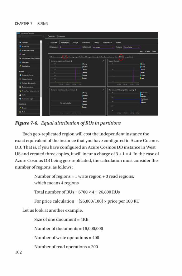
162
Each geo-replicated region will cost the independent instance the
exact equivalent of the instance that you have configured in Azure Cosmos
DB. That is, if you have configured an Azure Cosmos DB instance in West
US and created three copies, it will incur a charge of 3 + 1 = 4. In the case of
Azure Cosmos DB being geo-replicated, the calculation must consider the
number of regions, as follows:
Number of regions = 1 write region + 3 read regions,
which means 4 regions
Total number of RUs = 6700 × 4 = 26,800 RUs
For price calculation = (26,800/100) × price per 100 RU
Let us look at another example.
Size of one document = 4KB
Number of documents = 16,000,000
Number of write operations = 400
Number of read operations = 200
Figure 7-6. Equal distribution of RUs in partitions
Chapter 7 Sizing
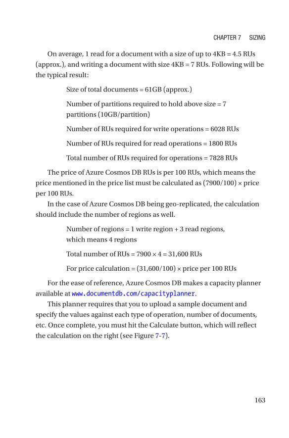
163
On average, 1 read for a document with a size of up to 4KB = 4.5 RUs
(approx.), and writing a document with size 4KB = 7 RUs. Following will be
the typical result:
Size of total documents = 61GB (approx.)
Number of partitions required to hold above size = 7
partitions (10GB/partition)
Number of RUs required for write operations = 6028 RUs
Number of RUs required for read operations = 1800 RUs
Total number of RUs required for operations = 7828 RUs
The price of Azure Cosmos DB RUs is per 100 RUs, which means the
price mentioned in the price list must be calculated as (7900/100) × price
per 100 RUs.
In the case of Azure Cosmos DB being geo-replicated, the calculation
should include the number of regions as well.
Number of regions = 1 write region + 3 read regions,
which means 4 regions
Total number of RUs = 7900 × 4 = 31,600 RUs
For price calculation = (31,600/100) × price per 100 RUs
For the ease of reference, Azure Cosmos DB makes a capacity planner
available at www.documentdb.com/capacityplanner.
This planner requires that you to upload a sample document and
specify the values against each type of operation, number of documents,
etc. Once complete, you must hit the Calculate button, which will reflect
the calculation on the right (see Figure 7-7).
Chapter 7 Sizing
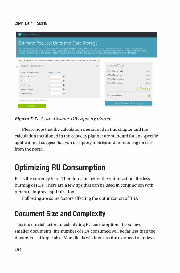
164
Please note that the calculation mentioned in this chapter and the
calculation mentioned in the capacity planner are standard for any specific
application. I suggest that you use query metrics and monitoring metrics
from the portal.
Optimizing RU ConsumptionRU is the currency here. Therefore, the better the optimization, the less
burning of RUs. There are a few tips that can be used in conjunction with
others to improve optimization.
Following are some factors affecting the optimization of RUs.
Document Size and Complexity This is a crucial factor for calculating RU consumption. If you have
smaller documents, the number of RUs consumed will be far less than the
documents of larger size. More fields will increase the overhead of indexes.
Figure 7-7. Azure Cosmos DB capacity planner
Chapter 7 Sizing
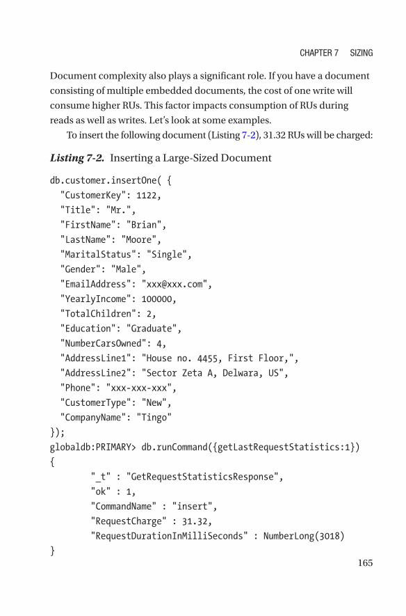
165
Document complexity also plays a significant role. If you have a document
consisting of multiple embedded documents, the cost of one write will
consume higher RUs. This factor impacts consumption of RUs during
reads as well as writes. Let’s look at some examples.
To insert the following document (Listing 7-2), 31.32 RUs will be charged:
Listing 7-2. Inserting a Large-Sized Document
db.customer.insertOne( {
"CustomerKey": 1122,
"Title": "Mr.",
"FirstName": "Brian",
"LastName": "Moore",
"MaritalStatus": "Single",
"Gender": "Male",
"EmailAddress": "[email protected]",
"YearlyIncome": 100000,
"TotalChildren": 2,
"Education": "Graduate",
"NumberCarsOwned": 4,
"AddressLine1": "House no. 4455, First Floor,",
"AddressLine2": "Sector Zeta A, Delwara, US",
"Phone": "xxx-xxx-xxx",
"CustomerType": "New",
"CompanyName": "Tingo"
});
globaldb:PRIMARY> db.runCommand({getLastRequestStatistics:1})
{
"_t" : "GetRequestStatisticsResponse",
"ok" : 1,
"CommandName" : "insert",
"RequestCharge" : 31.32,
"RequestDurationInMilliSeconds" : NumberLong(3018)
}
Chapter 7 Sizing
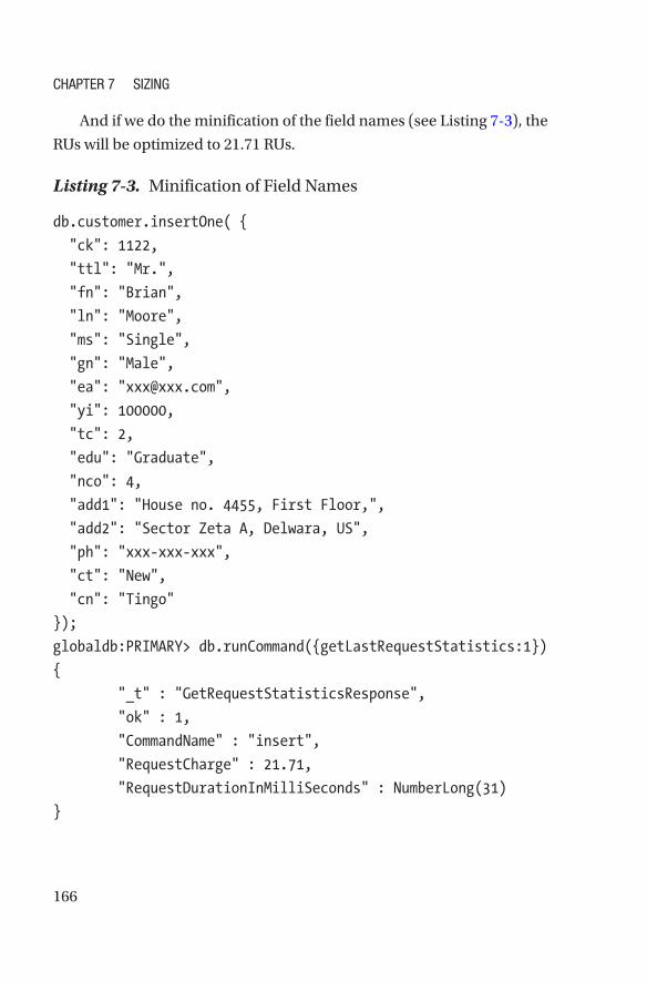
166
And if we do the minification of the field names (see Listing 7-3), the
RUs will be optimized to 21.71 RUs.
Listing 7-3. Minification of Field Names
db.customer.insertOne( {
"ck": 1122,
"ttl": "Mr.",
"fn": "Brian",
"ln": "Moore",
"ms": "Single",
"gn": "Male",
"ea": "[email protected]",
"yi": 100000,
"tc": 2,
"edu": "Graduate",
"nco": 4,
"add1": "House no. 4455, First Floor,",
"add2": "Sector Zeta A, Delwara, US",
"ph": "xxx-xxx-xxx",
"ct": "New",
"cn": "Tingo"
});
globaldb:PRIMARY> db.runCommand({getLastRequestStatistics:1})
{
"_t" : "GetRequestStatisticsResponse",
"ok" : 1,
"CommandName" : "insert",
"RequestCharge" : 21.71,
"RequestDurationInMilliSeconds" : NumberLong(31)
}
Chapter 7 Sizing
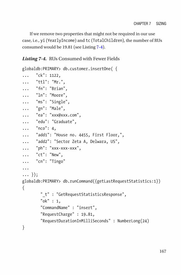
167
If we remove two properties that might not be required in our use
case, i.e., yi (YearlyIncome) and tc (TotalChildren), the number of RUs
consumed would be 19.81 (see Listing 7-4).
Listing 7-4. RUs Consumed with Fewer Fields
globaldb:PRIMARY> db.customer.insertOne( {
... "ck": 1122,
... "ttl": "Mr.",
... "fn": "Brian",
... "ln": "Moore",
... "ms": "Single",
... "gn": "Male",
... "ea": "[email protected]",
... "edu": "Graduate",
... "nco": 4,
... "add1": "House no. 4455, First Floor,",
... "add2": "Sector Zeta A, Delwara, US",
... "ph": "xxx-xxx-xxx",
... "ct": "New",
... "cn": "Tingo"
...
... });
globaldb:PRIMARY> db.runCommand({getLastRequestStatistics:1})
{
"_t" : "GetRequestStatisticsResponse",
"ok" : 1,
"CommandName" : "insert",
"RequestCharge" : 19.81,
"RequestDurationInMilliSeconds" : NumberLong(24)
}
Chapter 7 Sizing
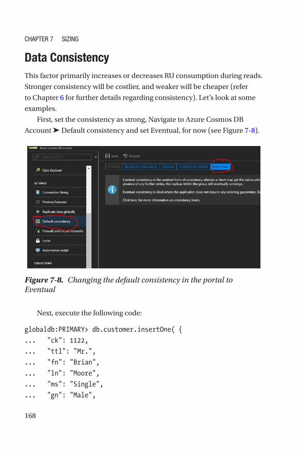
168
Data Consistency This factor primarily increases or decreases RU consumption during reads.
Stronger consistency will be costlier, and weaker will be cheaper (refer
to Chapter 6 for further details regarding consistency). Let’s look at some
examples.
First, set the consistency as strong, Navigate to Azure Cosmos DB
Account ➤ Default consistency and set Eventual, for now (see Figure 7-8).
Next, execute the following code:
globaldb:PRIMARY> db.customer.insertOne( {
... "ck": 1122,
... "ttl": "Mr.",
... "fn": "Brian",
... "ln": "Moore",
... "ms": "Single",
... "gn": "Male",
Figure 7-8. Changing the default consistency in the portal to Eventual
Chapter 7 Sizing
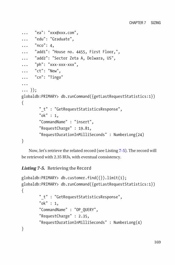
169
... "ea": "[email protected]",
... "edu": "Graduate",
... "nco": 4,
... "add1": "House no. 4455, First Floor,",
... "add2": "Sector Zeta A, Delwara, US",
... "ph": "xxx-xxx-xxx",
... "ct": "New",
... "cn": "Tingo"
...
... });
globaldb:PRIMARY> db.runCommand({getLastRequestStatistics:1})
{
"_t" : "GetRequestStatisticsResponse",
"ok" : 1,
"CommandName" : "insert",
"RequestCharge" : 19.81,
"RequestDurationInMilliSeconds" : NumberLong(24)
}
Now, let’s retrieve the related record (see Listing 7-5). The record will
be retrieved with 2.35 RUs, with eventual consistency.
Listing 7-5. Retrieving the Record
globaldb:PRIMARY> db.customer.find({}).limit(1);
globaldb:PRIMARY> db.runCommand({getLastRequestStatistics:1})
{
"_t" : "GetRequestStatisticsResponse",
"ok" : 1,
"CommandName" : "OP_QUERY",
"RequestCharge" : 2.35,
"RequestDurationInMilliSeconds" : NumberLong(4)
}
Chapter 7 Sizing
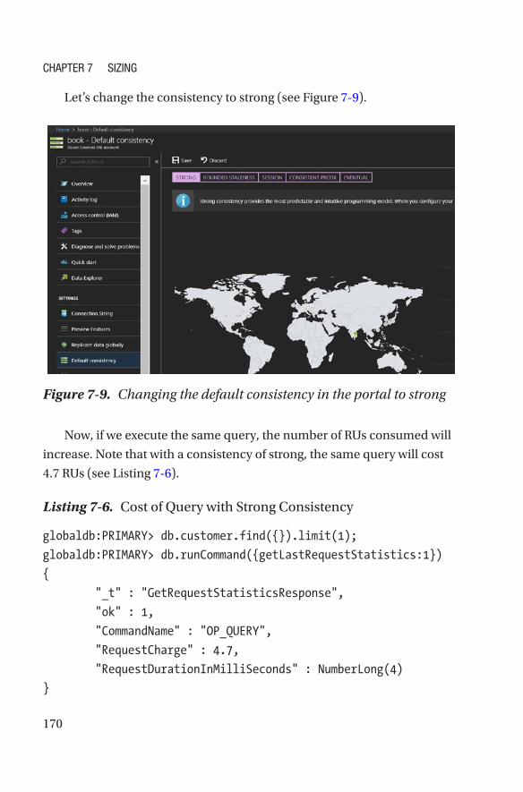
170
Let’s change the consistency to strong (see Figure 7-9).
Now, if we execute the same query, the number of RUs consumed will
increase. Note that with a consistency of strong, the same query will cost
4.7 RUs (see Listing 7-6).
Listing 7-6. Cost of Query with Strong Consistency
globaldb:PRIMARY> db.customer.find({}).limit(1);
globaldb:PRIMARY> db.runCommand({getLastRequestStatistics:1})
{
"_t" : "GetRequestStatisticsResponse",
"ok" : 1,
"CommandName" : "OP_QUERY",
"RequestCharge" : 4.7,
"RequestDurationInMilliSeconds" : NumberLong(4)
}
Figure 7-9. Changing the default consistency in the portal to strong
Chapter 7 Sizing
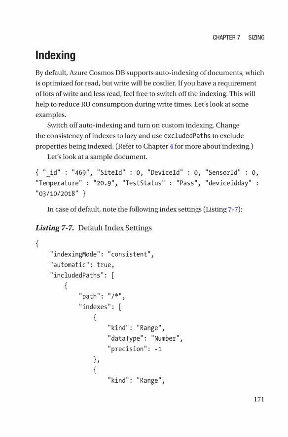
171
Indexing By default, Azure Cosmos DB supports auto-indexing of documents, which
is optimized for read, but write will be costlier. If you have a requirement
of lots of write and less read, feel free to switch off the indexing. This will
help to reduce RU consumption during write times. Let’s look at some
examples.
Switch off auto-indexing and turn on custom indexing. Change
the consistency of indexes to lazy and use excludedPaths to exclude
properties being indexed. (Refer to Chapter 4 for more about indexing.)
Let’s look at a sample document.
{ "_id" : "469", "SiteId" : 0, "DeviceId" : 0, "SensorId" : 0,
"Temperature" : "20.9", "TestStatus" : "Pass", "deviceidday" :
"03/10/2018" }
In case of default, note the following index settings (Listing 7-7):
Listing 7-7. Default Index Settings
{
"indexingMode": "consistent",
"automatic": true,
"includedPaths": [
{
"path": "/*",
"indexes": [
{
"kind": "Range",
"dataType": "Number",
"precision": -1
},
{
"kind": "Range",
Chapter 7 Sizing
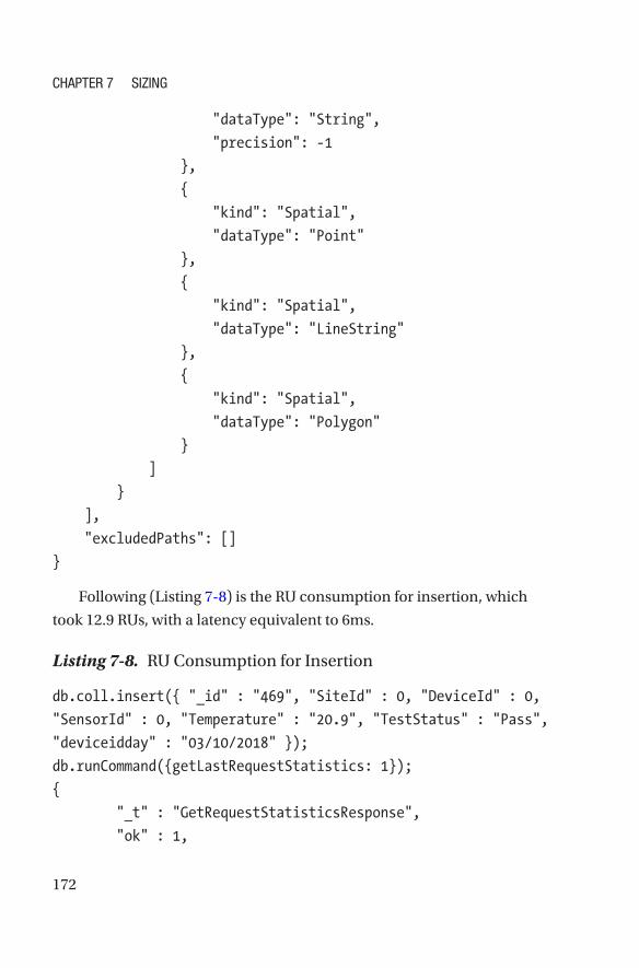
172
"dataType": "String",
"precision": -1
},
{
"kind": "Spatial",
"dataType": "Point"
},
{
"kind": "Spatial",
"dataType": "LineString"
},
{
"kind": "Spatial",
"dataType": "Polygon"
}
]
}
],
"excludedPaths": []
}
Following (Listing 7-8) is the RU consumption for insertion, which
took 12.9 RUs, with a latency equivalent to 6ms.
Listing 7-8. RU Consumption for Insertion
db.coll.insert({ "_id" : "469", "SiteId" : 0, "DeviceId" : 0,
"SensorId" : 0, "Temperature" : "20.9", "TestStatus" : "Pass",
"deviceidday" : "03/10/2018" });
db.runCommand({getLastRequestStatistics: 1});
{
"_t" : "GetRequestStatisticsResponse",
"ok" : 1,
Chapter 7 Sizing
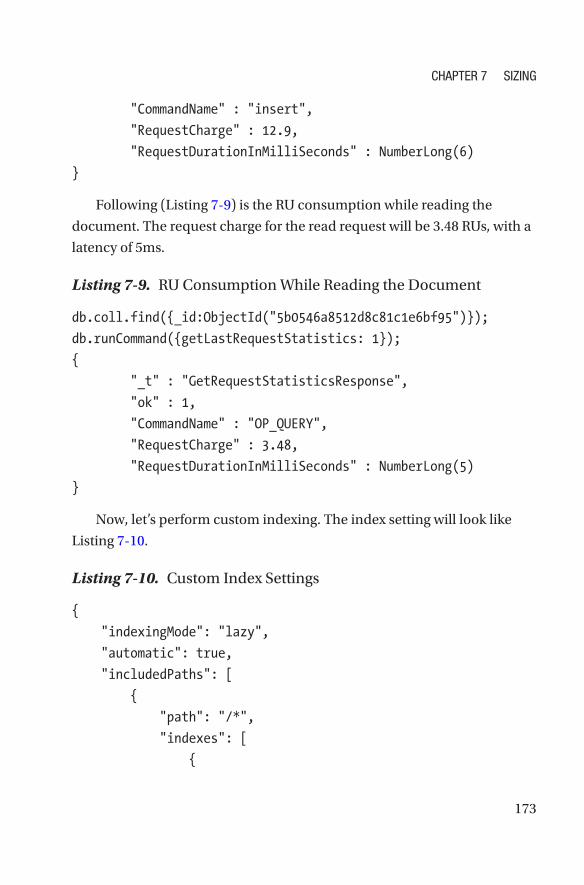
173
"CommandName" : "insert",
"RequestCharge" : 12.9,
"RequestDurationInMilliSeconds" : NumberLong(6)
}
Following (Listing 7-9) is the RU consumption while reading the
document. The request charge for the read request will be 3.48 RUs, with a
latency of 5ms.
Listing 7-9. RU Consumption While Reading the Document
db.coll.find({_id:ObjectId("5b0546a8512d8c81c1e6bf95")});
db.runCommand({getLastRequestStatistics: 1});
{
"_t" : "GetRequestStatisticsResponse",
"ok" : 1,
"CommandName" : "OP_QUERY",
"RequestCharge" : 3.48,
"RequestDurationInMilliSeconds" : NumberLong(5)
}
Now, let’s perform custom indexing. The index setting will look like
Listing 7-10.
Listing 7-10. Custom Index Settings
{
"indexingMode": "lazy",
"automatic": true,
"includedPaths": [
{
"path": "/*",
"indexes": [
{
Chapter 7 Sizing
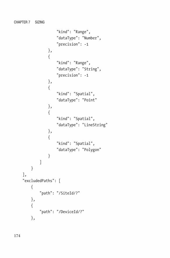
174
"kind": "Range",
"dataType": "Number",
"precision": -1
},
{
"kind": "Range",
"dataType": "String",
"precision": -1
},
{
"kind": "Spatial",
"dataType": "Point"
},
{
"kind": "Spatial",
"dataType": "LineString"
},
{
"kind": "Spatial",
"dataType": "Polygon"
}
]
}
],
"excludedPaths": [
{
"path": "/SiteId/?"
},
{
"path": "/DeviceId/?"
},
Chapter 7 Sizing
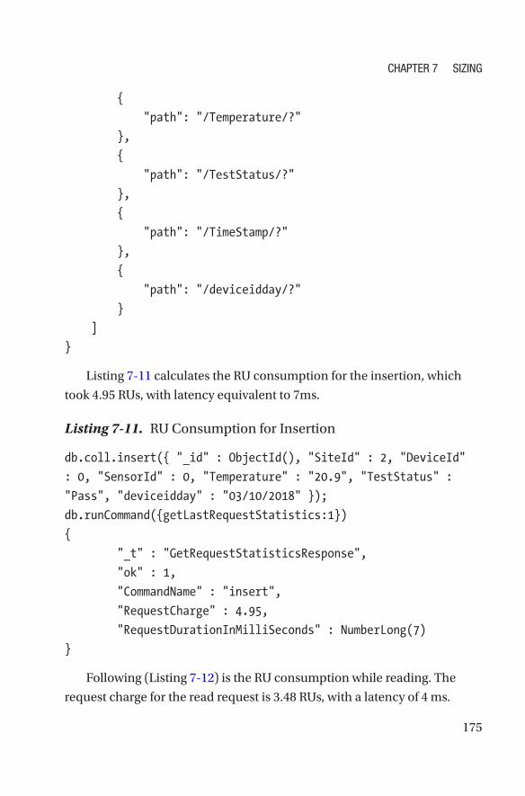
175
{
"path": "/Temperature/?"
},
{
"path": "/TestStatus/?"
},
{
"path": "/TimeStamp/?"
},
{
"path": "/deviceidday/?"
}
]
}
Listing 7-11 calculates the RU consumption for the insertion, which
took 4.95 RUs, with latency equivalent to 7ms.
Listing 7-11. RU Consumption for Insertion
db.coll.insert({ "_id" : ObjectId(), "SiteId" : 2, "DeviceId"
: 0, "SensorId" : 0, "Temperature" : "20.9", "TestStatus" :
"Pass", "deviceidday" : "03/10/2018" });
db.runCommand({getLastRequestStatistics:1})
{
"_t" : "GetRequestStatisticsResponse",
"ok" : 1,
"CommandName" : "insert",
"RequestCharge" : 4.95,
"RequestDurationInMilliSeconds" : NumberLong(7)
}
Following (Listing 7-12) is the RU consumption while reading. The
request charge for the read request is 3.48 RUs, with a latency of 4 ms.
Chapter 7 Sizing
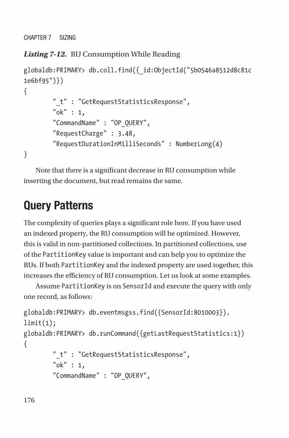
176
Listing 7-12. RU Consumption While Reading
globaldb:PRIMARY> db.coll.find({_id:ObjectId("5b0546a8512d8c81c
1e6bf95")})
{
"_t" : "GetRequestStatisticsResponse",
"ok" : 1,
"CommandName" : "OP_QUERY",
"RequestCharge" : 3.48,
"RequestDurationInMilliSeconds" : NumberLong(4)
}
Note that there is a significant decrease in RU consumption while
inserting the document, but read remains the same.
Query Patterns The complexity of queries plays a significant role here. If you have used
an indexed property, the RU consumption will be optimized. However,
this is valid in non-partitioned collections. In partitioned collections, use
of the PartitionKey value is important and can help you to optimize the
RUs. If both PartitionKey and the indexed property are used together, this
increases the efficiency of RU consumption. Let us look at some examples.
Assume PartitionKey is on SensorId and execute the query with only
one record, as follows:
globaldb:PRIMARY> db.eventmsgss.find({SensorId:8010003}).
limit(1);
globaldb:PRIMARY> db.runCommand({getLastRequestStatistics:1})
{
"_t" : "GetRequestStatisticsResponse",
"ok" : 1,
"CommandName" : "OP_QUERY",
Chapter 7 Sizing
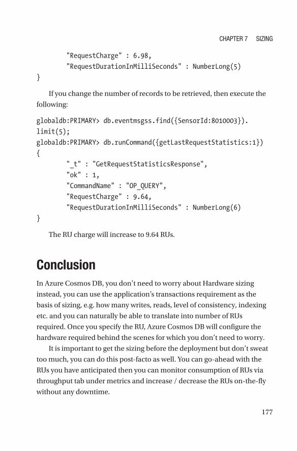
177
"RequestCharge" : 6.98,
"RequestDurationInMilliSeconds" : NumberLong(5)
}
If you change the number of records to be retrieved, then execute the
following:
globaldb:PRIMARY> db.eventmsgss.find({SensorId:8010003}).
limit(5);
globaldb:PRIMARY> db.runCommand({getLastRequestStatistics:1})
{
"_t" : "GetRequestStatisticsResponse",
"ok" : 1,
"CommandName" : "OP_QUERY",
"RequestCharge" : 9.64,
"RequestDurationInMilliSeconds" : NumberLong(6)
}
The RU charge will increase to 9.64 RUs.
ConclusionIn Azure Cosmos DB, you don’t need to worry about Hardware sizing
instead, you can use the application’s transactions requirement as the
basis of sizing, e.g. how many writes, reads, level of consistency, indexing
etc. and you can naturally be able to translate into number of RUs
required. Once you specify the RU, Azure Cosmos DB will configure the
hardware required behind the scenes for which you don’t need to worry.
It is important to get the sizing before the deployment but don’t sweat
too much, you can do this post-facto as well. You can go-ahead with the
RUs you have anticipated then you can monitor consumption of RUs via
throughput tab under metrics and increase / decrease the RUs on-the-fly
without any downtime.
Chapter 7 Sizing
179© Manish Sharma 2018 M. Sharma, Cosmos DB for MongoDB Developers, https://doi.org/10.1007/978-1-4842-3682-6_8
CHAPTER 8
Migrating to Azure Cosmos DB–MongoDB APINow that I have covered most of the aspects of Azure Cosmos
DB–MongoDB API, in this chapter, we will delve into the actual logistics of
migrating an entire application to Azure Cosmos DB–MongoDB API.
Migration StrategiesMany strategies exist to migrate NoSQL data from one database to another
type of database. The major worry for a developer while migrating from
one technology to another is to ensure compatibility between the target
and source. With protocol support, Azure Cosmos DB with Mongo API
tries to resolve the compatibility issues. Ideally, you should be changing
only the connection string, which is available mostly in the configuration
file, and you can easily replace it. But there are a few instances in which
you must change the code, as there are commands that are not supported
here, e.g., $text, $pull with condition, etc. You can access the MongoDB
API support page at https://aka.ms/mongodb-feature-support for the
most updated list of commands supported.
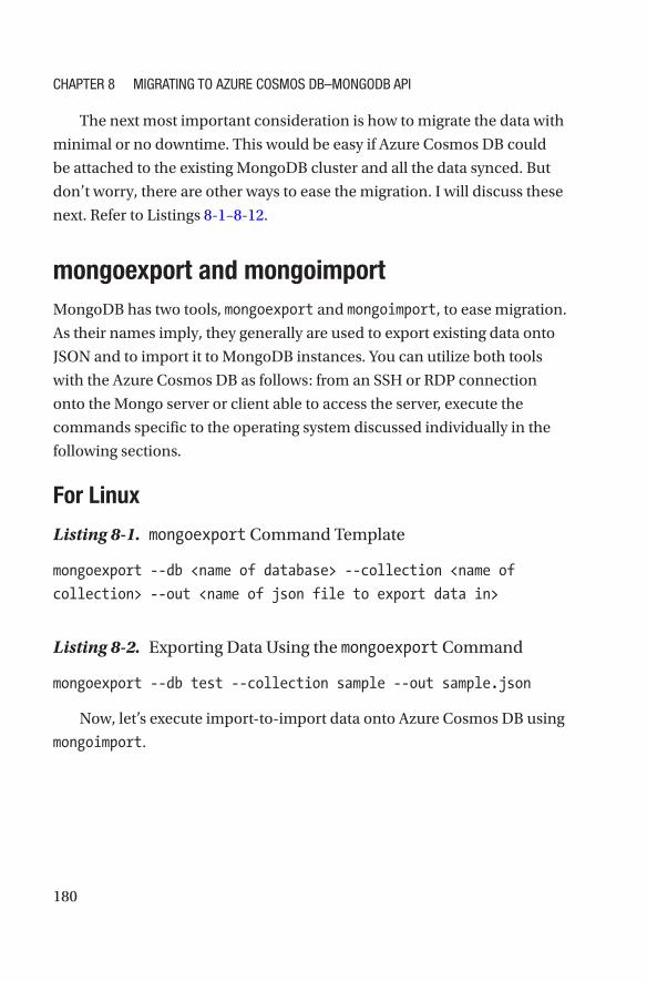
180
The next most important consideration is how to migrate the data with
minimal or no downtime. This would be easy if Azure Cosmos DB could
be attached to the existing MongoDB cluster and all the data synced. But
don’t worry, there are other ways to ease the migration. I will discuss these
next. Refer to Listings 8-1–8-12.
mongoexport and mongoimportMongoDB has two tools, mongoexport and mongoimport, to ease migration.
As their names imply, they generally are used to export existing data onto
JSON and to import it to MongoDB instances. You can utilize both tools
with the Azure Cosmos DB as follows: from an SSH or RDP connection
onto the Mongo server or client able to access the server, execute the
commands specific to the operating system discussed individually in the
following sections.
For Linux
Listing 8-1. mongoexport Command Template
mongoexport --db <name of database> --collection <name of
collection> --out <name of json file to export data in>
Listing 8-2. Exporting Data Using the mongoexport Command
mongoexport --db test --collection sample --out sample.json
Now, let’s execute import-to-import data onto Azure Cosmos DB using
mongoimport.
Chapter 8 Migrating to azure CosMos DB–MongoDB api
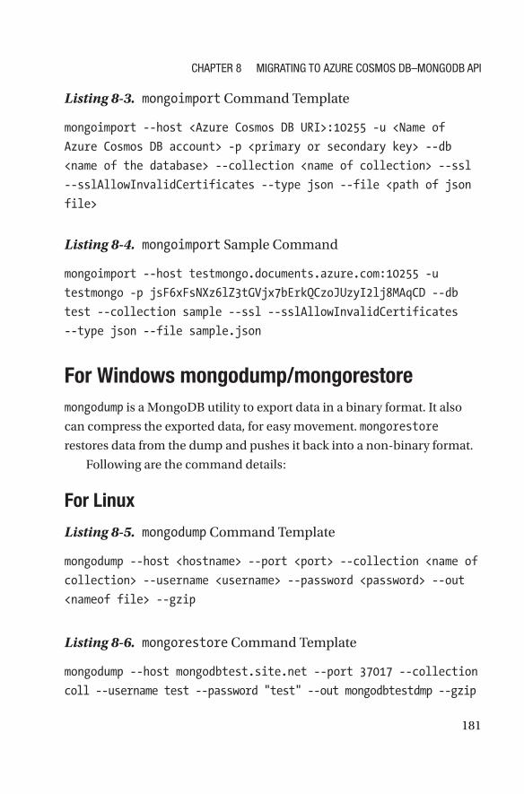
181
Listing 8-3. mongoimport Command Template
mongoimport --host <Azure Cosmos DB URI>:10255 -u <Name of
Azure Cosmos DB account> -p <primary or secondary key> --db
<name of the database> --collection <name of collection> --ssl
--sslAllowInvalidCertificates --type json --file <path of json
file>
Listing 8-4. mongoimport Sample Command
mongoimport --host testmongo.documents.azure.com:10255 -u
testmongo -p jsF6xFsNXz6lZ3tGVjx7bErkQCzoJUzyI2lj8MAqCD --db
test --collection sample --ssl --sslAllowInvalidCertificates
--type json --file sample.json
For Windows mongodump/mongorestoremongodump is a MongoDB utility to export data in a binary format. It also
can compress the exported data, for easy movement. mongorestore
restores data from the dump and pushes it back into a non-binary format.
Following are the command details:
For Linux
Listing 8-5. mongodump Command Template
mongodump --host <hostname> --port <port> --collection <name of
collection> --username <username> --password <password> --out
<nameof file> --gzip
Listing 8-6. mongorestore Command Template
mongodump --host mongodbtest.site.net --port 37017 --collection
coll --username test --password "test" --out mongodbtestdmp --gzip
Chapter 8 Migrating to azure CosMos DB–MongoDB api
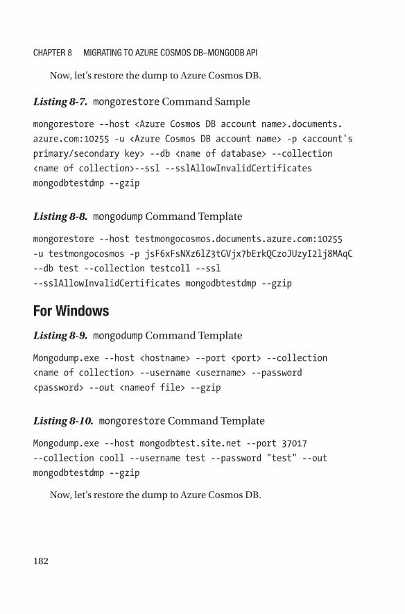
182
Now, let’s restore the dump to Azure Cosmos DB.
Listing 8-7. mongorestore Command Sample
mongorestore --host <Azure Cosmos DB account name>.documents.
azure.com:10255 -u <Azure Cosmos DB account name> -p <account's
primary/secondary key> --db <name of database> --collection
<name of collection>--ssl --sslAllowInvalidCertificates
mongodbtestdmp --gzip
Listing 8-8. mongodump Command Template
mongorestore --host testmongocosmos.documents.azure.com:10255
-u testmongocosmos -p jsF6xFsNXz6lZ3tGVjx7bErkQCzoJUzyI2lj8MAqC
--db test --collection testcoll --ssl
--sslAllowInvalidCertificates mongodbtestdmp --gzip
For Windows
Listing 8-9. mongodump Command Template
Mongodump.exe --host <hostname> --port <port> --collection
<name of collection> --username <username> --password
<password> --out <nameof file> --gzip
Listing 8-10. mongorestore Command Template
Mongodump.exe --host mongodbtest.site.net --port 37017
--collection cooll --username test --password "test" --out
mongodbtestdmp --gzip
Now, let’s restore the dump to Azure Cosmos DB.
Chapter 8 Migrating to azure CosMos DB–MongoDB api
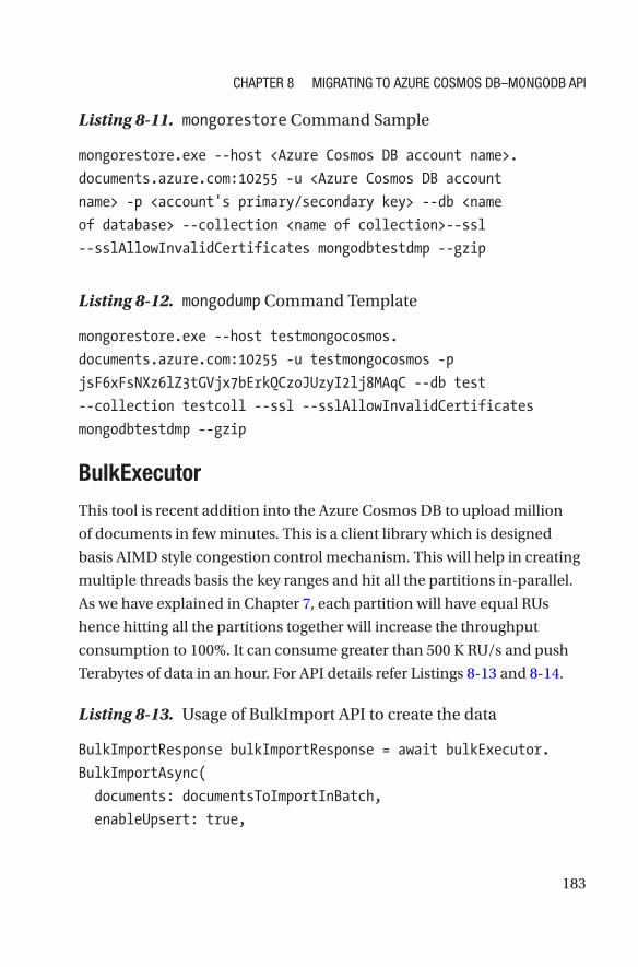
183
Listing 8-11. mongorestore Command Sample
mongorestore.exe --host <Azure Cosmos DB account name>.
documents.azure.com:10255 -u <Azure Cosmos DB account
name> -p <account's primary/secondary key> --db <name
of database> --collection <name of collection>--ssl
--sslAllowInvalidCertificates mongodbtestdmp --gzip
Listing 8-12. mongodump Command Template
mongorestore.exe --host testmongocosmos.
documents.azure.com:10255 -u testmongocosmos -p
jsF6xFsNXz6lZ3tGVjx7bErkQCzoJUzyI2lj8MAqC --db test
--collection testcoll --ssl --sslAllowInvalidCertificates
mongodbtestdmp --gzip
BulkExecutor
This tool is recent addition into the Azure Cosmos DB to upload million
of documents in few minutes. This is a client library which is designed
basis AIMD style congestion control mechanism. This will help in creating
multiple threads basis the key ranges and hit all the partitions in-parallel.
As we have explained in Chapter 7, each partition will have equal RUs
hence hitting all the partitions together will increase the throughput
consumption to 100%. It can consume greater than 500 K RU/s and push
Terabytes of data in an hour. For API details refer Listings 8-13 and 8-14.
Listing 8-13. Usage of BulkImport API to create the data
BulkImportResponse bulkImportResponse = await bulkExecutor.
BulkImportAsync(
documents: documentsToImportInBatch,
enableUpsert: true,
Chapter 8 Migrating to azure CosMos DB–MongoDB api
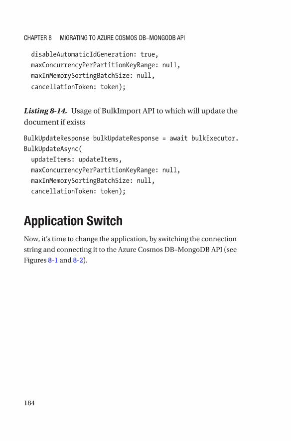
184
disableAutomaticIdGeneration: true,
maxConcurrencyPerPartitionKeyRange: null,
maxInMemorySortingBatchSize: null,
cancellationToken: token);
Listing 8-14. Usage of BulkImport API to which will update the
document if exists
BulkUpdateResponse bulkUpdateResponse = await bulkExecutor.
BulkUpdateAsync(
updateItems: updateItems,
maxConcurrencyPerPartitionKeyRange: null,
maxInMemorySortingBatchSize: null,
cancellationToken: token);
Application SwitchNow, it’s time to change the application, by switching the connection
string and connecting it to the Azure Cosmos DB–MongoDB API (see
Figures 8-1 and 8-2).
Chapter 8 Migrating to azure CosMos DB–MongoDB api
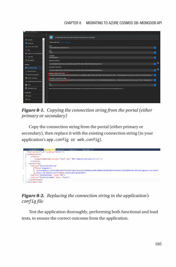
185
Copy the connection string from the portal (either primary or
secondary), then replace it with the existing connection string (in your
application’s app.config or web.config).
Figure 8-1. Copying the connection string from the portal (either primary or secondary)
Figure 8-2. Replacing the connection string in the application’s config file
Test the application thoroughly, performing both functional and load
tests, to ensure the correct outcome from the application.
Chapter 8 Migrating to azure CosMos DB–MongoDB api
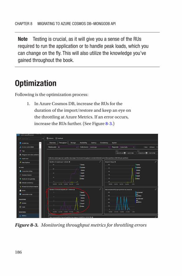
186
Note testing is crucial, as it will give you a sense of the rus required to run the application or to handle peak loads, which you can change on the fly. this will also utilize the knowledge you’ve gained throughout the book.
OptimizationFollowing is the optimization process:
1. In Azure Cosmos DB, increase the RUs for the
duration of the import/restore and keep an eye on
the throttling at Azure Metrics. If an error occurs,
increase the RUs further. (See Figure 8-3.)
Figure 8-3. Monitoring throughput metrics for throttling errors
Chapter 8 Migrating to azure CosMos DB–MongoDB api
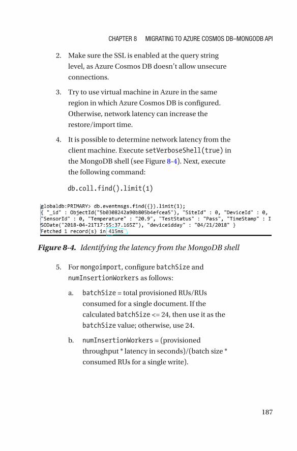
187
2. Make sure the SSL is enabled at the query string
level, as Azure Cosmos DB doesn’t allow unsecure
connections.
3. Try to use virtual machine in Azure in the same
region in which Azure Cosmos DB is configured.
Otherwise, network latency can increase the
restore/import time.
4. It is possible to determine network latency from the
client machine. Execute setVerboseShell(true) in
the MongoDB shell (see Figure 8- 4). Next, execute
the following command:
db.coll.find().limit(1)
Figure 8-4. Identifying the latency from the MongoDB shell
5. For mongoimport, configure batchSize and
numInsertionWorkers as follows:
a. batchSize = total provisioned RUs/RUs
consumed for a single document. If the
calculated batchSize <= 24, then use it as the
batchSize value; otherwise, use 24.
b. numInsertionWorkers = (provisioned
throughput * latency in seconds)/(batch size *
consumed RUs for a single write).
Chapter 8 Migrating to azure CosMos DB–MongoDB api
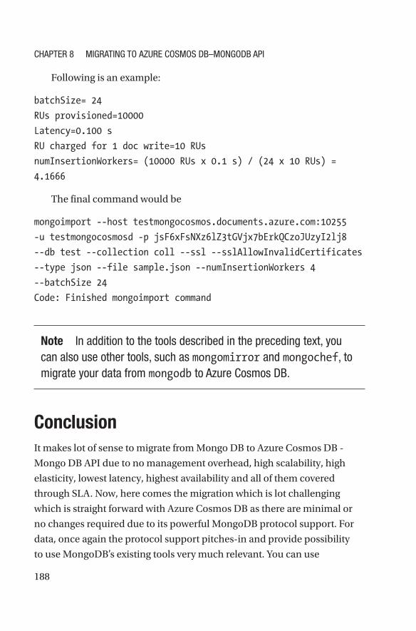
188
Following is an example:
batchSize= 24
RUs provisioned=10000
Latency=0.100 s
RU charged for 1 doc write=10 RUs
numInsertionWorkers= (10000 RUs x 0.1 s) / (24 x 10 RUs) =
4.1666
The final command would be
mongoimport --host testmongocosmos.documents.azure.com:10255
-u testmongocosmosd -p jsF6xFsNXz6lZ3tGVjx7bErkQCzoJUzyI2lj8
--db test --collection coll --ssl --sslAllowInvalidCertificates
--type json --file sample.json --numInsertionWorkers 4
--batchSize 24
Code: Finished mongoimport command
Note in addition to the tools described in the preceding text, you can also use other tools, such as mongomirror and mongochef, to migrate your data from mongodb to azure Cosmos DB.
ConclusionIt makes lot of sense to migrate from Mongo DB to Azure Cosmos DB -
Mongo DB API due to no management overhead, high scalability, high
elasticity, lowest latency, highest availability and all of them covered
through SLA. Now, here comes the migration which is lot challenging
which is straight forward with Azure Cosmos DB as there are minimal or
no changes required due to its powerful MongoDB protocol support. For
data, once again the protocol support pitches-in and provide possibility
to use MongoDB’s existing tools very much relevant. You can use
Chapter 8 Migrating to azure CosMos DB–MongoDB api
189
MongoDB’s shell command import/export, restore or their OOTB tools
e.g. mongomirror, mongochef etc. Recently, there is an introduction of
BulkExecutor tool which will make data push as parallel and reduce time
push data as optimize as 40 - 50 times.
In next chapter we will look into advanced functionalities e.g. Spark,
Aggregation pipeline etc.
Chapter 8 Migrating to azure CosMos DB–MongoDB api
191© Manish Sharma 2018 M. Sharma, Cosmos DB for MongoDB Developers, https://doi.org/10.1007/978-1-4842-3682-6_9
CHAPTER 9
Azure Cosmos DB–MongoDB API Advanced ServicesFinally, we have reached the last chapter in our journey, and I would like
to share some of the important points that are applicable in day-to-day
scenarios.
Aggregation PipelineThis is the inherent feature in MongoDB that is critical for the workloads
that require analytics and specific aggregation. In Azure Cosmos DB, the
data aggregation pipeline is supported. However, at the time of writing
this book, it was out for public preview and must be enabled explicitly
by navigating to the preview items in the Azure portal, under the Azure
Cosmos DB blade.
Now, let’s get our hands dirty. Open your favorite MongoDB console
and connect to Azure Cosmos DB.
sudo mongo <Azure Cosmos DB Account Name>.documents.azure.
com:10255/db -u < Azure Cosmos DB Account Name > -p <primary/
secondary key> --ssl --sslAllowInvalidCertificates
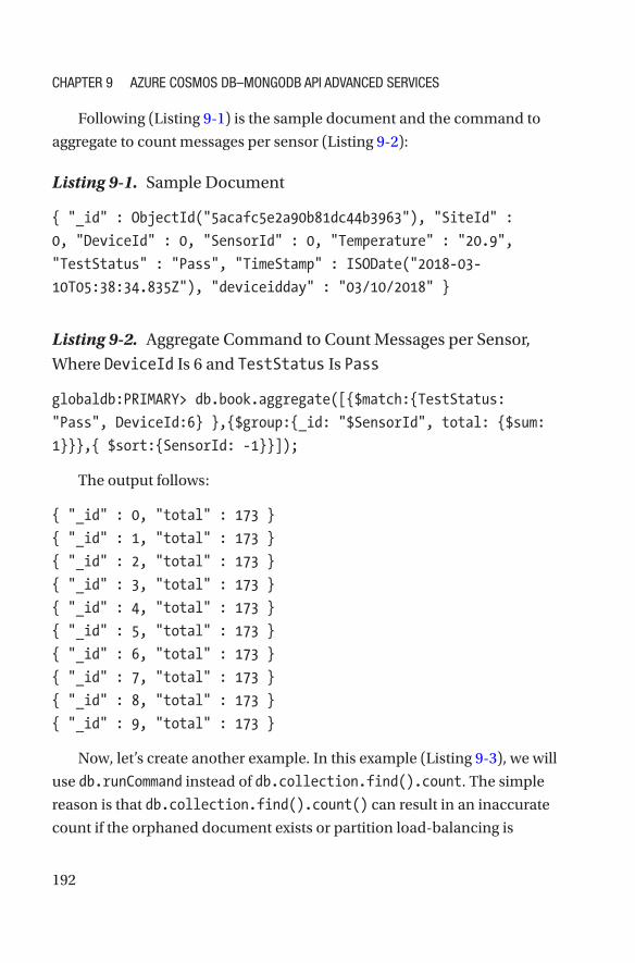
192
Following (Listing 9-1) is the sample document and the command to
aggregate to count messages per sensor (Listing 9-2):
Listing 9-1. Sample Document
{ "_id" : ObjectId("5acafc5e2a90b81dc44b3963"), "SiteId" :
0, "DeviceId" : 0, "SensorId" : 0, "Temperature" : "20.9",
"TestStatus" : "Pass", "TimeStamp" : ISODate("2018-03-
10T05:38:34.835Z"), "deviceidday" : "03/10/2018" }
Listing 9-2. Aggregate Command to Count Messages per Sensor,
Where DeviceId Is 6 and TestStatus Is Pass
globaldb:PRIMARY> db.book.aggregate([{$match:{TestStatus:
"Pass", DeviceId:6} },{$group:{_id: "$SensorId", total: {$sum:
1}}},{ $sort:{SensorId: -1}}]);
The output follows:
{ "_id" : 0, "total" : 173 }
{ "_id" : 1, "total" : 173 }
{ "_id" : 2, "total" : 173 }
{ "_id" : 3, "total" : 173 }
{ "_id" : 4, "total" : 173 }
{ "_id" : 5, "total" : 173 }
{ "_id" : 6, "total" : 173 }
{ "_id" : 7, "total" : 173 }
{ "_id" : 8, "total" : 173 }
{ "_id" : 9, "total" : 173 }
Now, let’s create another example. In this example (Listing 9-3), we will
use db.runCommand instead of db.collection.find().count. The simple
reason is that db.collection.find().count() can result in an inaccurate
count if the orphaned document exists or partition load-balancing is
Chapter 9 azure Cosmos DB–mongoDB apI aDvanCeD servICes
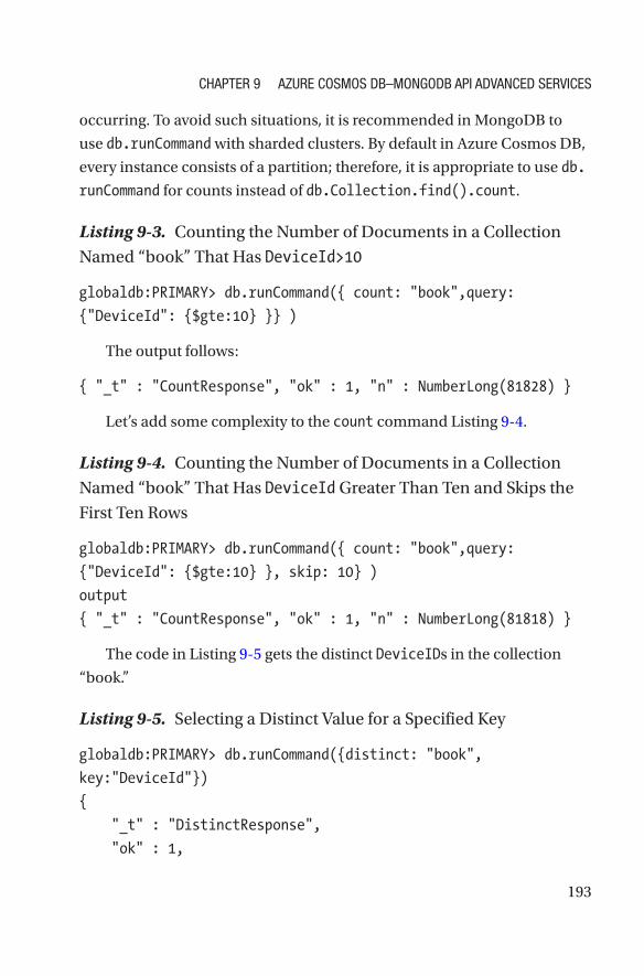
193
occurring. To avoid such situations, it is recommended in MongoDB to
use db.runCommand with sharded clusters. By default in Azure Cosmos DB,
every instance consists of a partition; therefore, it is appropriate to use db.
runCommand for counts instead of db.Collection.find().count.
Listing 9-3. Counting the Number of Documents in a Collection
Named “book” That Has DeviceId>10
globaldb:PRIMARY> db.runCommand({ count: "book",query:
{"DeviceId": {$gte:10} }} )
The output follows:
{ "_t" : "CountResponse", "ok" : 1, "n" : NumberLong(81828) }
Let’s add some complexity to the count command Listing 9-4.
Listing 9-4. Counting the Number of Documents in a Collection
Named “book” That Has DeviceId Greater Than Ten and Skips the
First Ten Rows
globaldb:PRIMARY> db.runCommand({ count: "book",query:
{"DeviceId": {$gte:10} }, skip: 10} )
output
{ "_t" : "CountResponse", "ok" : 1, "n" : NumberLong(81818) }
The code in Listing 9-5 gets the distinct DeviceIDs in the collection
“book.”
Listing 9-5. Selecting a Distinct Value for a Specified Key
globaldb:PRIMARY> db.runCommand({distinct: "book",
key:"DeviceId"})
{
"_t" : "DistinctResponse",
"ok" : 1,
Chapter 9 azure Cosmos DB–mongoDB apI aDvanCeD servICes
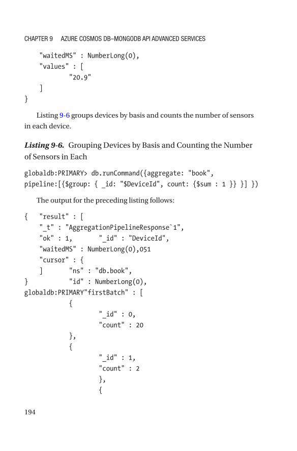
194
"waitedMS" : NumberLong(0),
"values" : [
"20.9"
]
}
Listing 9-6 groups devices by basis and counts the number of sensors
in each device.
Listing 9-6. Grouping Devices by Basis and Counting the Number
of Sensors in Each
globaldb:PRIMARY> db.runCommand({aggregate: "book",
pipeline:[{$group: { _id: "$DeviceId", count: {$sum : 1 }} }] })
The output for the preceding listing follows:
{ "result" : [
"_t" : "AggregationPipelineResponse`1",
"ok" : 1, "_id" : "DeviceId",
"waitedMS" : NumberLong(0),051
"cursor" : {
] "ns" : "db.book",
} "id" : NumberLong(0),
globaldb:PRIMARY"firstBatch" : [
{
"_id" : 0,
"count" : 20
},
{
"_id" : 1,
"count" : 2
},
{
Chapter 9 azure Cosmos DB–mongoDB apI aDvanCeD servICes
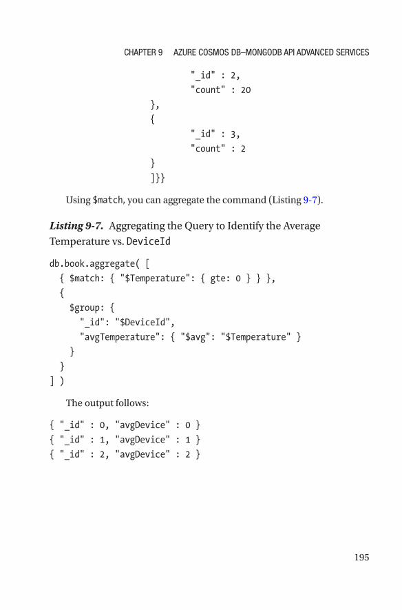
195
"_id" : 2,
"count" : 20
},
{
"_id" : 3,
"count" : 2
}
]}}
Using $match, you can aggregate the command (Listing 9-7).
Listing 9-7. Aggregating the Query to Identify the Average
Temperature vs. DeviceId
db.book.aggregate( [
{ $match: { "$Temperature": { gte: 0 } } },
{
$group: {
"_id": "$DeviceId",
"avgTemperature": { "$avg": "$Temperature" }
}
}
] )
The output follows:
{ "_id" : 0, "avgDevice" : 0 }
{ "_id" : 1, "avgDevice" : 1 }
{ "_id" : 2, "avgDevice" : 2 }
Chapter 9 azure Cosmos DB–mongoDB apI aDvanCeD servICes
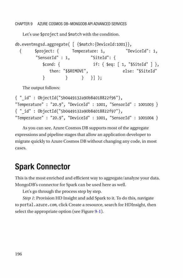
196
Let’s use $project and $match with the condition.
db.eventmsgsd.aggregate( [ {$match:{DeviceId:1001}},
{ $project: { Temperature: 1, "DeviceId": 1,
"SensorId" : 1, "SiteId": {
$cond: { if: { $eq: [ 1, "$SiteId" ] },
then: "$$REMOVE", else: "$SiteId"
} } } }] );
The output follows:
{ "_id" : ObjectId("5b0449132a90b84018822f96"),
"Temperature" : "20.9", "DeviceId" : 1001, "SensorId" : 1001003 }
{ "_id" : ObjectId("5b0449132a90b84018822f97"),
"Temperature" : "20.9", "DeviceId" : 1001, "SensorId" : 1001004 }
As you can see, Azure Cosmos DB supports most of the aggregate
expressions and pipeline stages that allow an application developer to
migrate quickly to Azure Cosmos DB without changing any code, in most
cases.
Spark ConnectorThis is the most enriched and efficient way to aggregate/analyze your data.
MongoDB’s connector for Spark can be used here as well.
Let’s go through the process step by step.
Step 1: Provision HD Insight and add Spark to it. To do this, navigate
to portal.azure.com, click Create a resource, search for HDInsight, then
select the appropriate option (see Figure 9-1).
Chapter 9 azure Cosmos DB–mongoDB apI aDvanCeD servICes
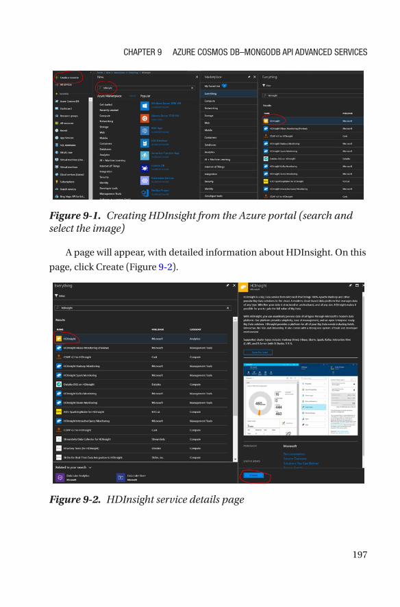
197
A page will appear, with detailed information about HDInsight. On this
page, click Create (Figure 9-2).
Figure 9-1. Creating HDInsight from the Azure portal (search and select the image)
Figure 9-2. HDInsight service details page
Chapter 9 azure Cosmos DB–mongoDB apI aDvanCeD servICes
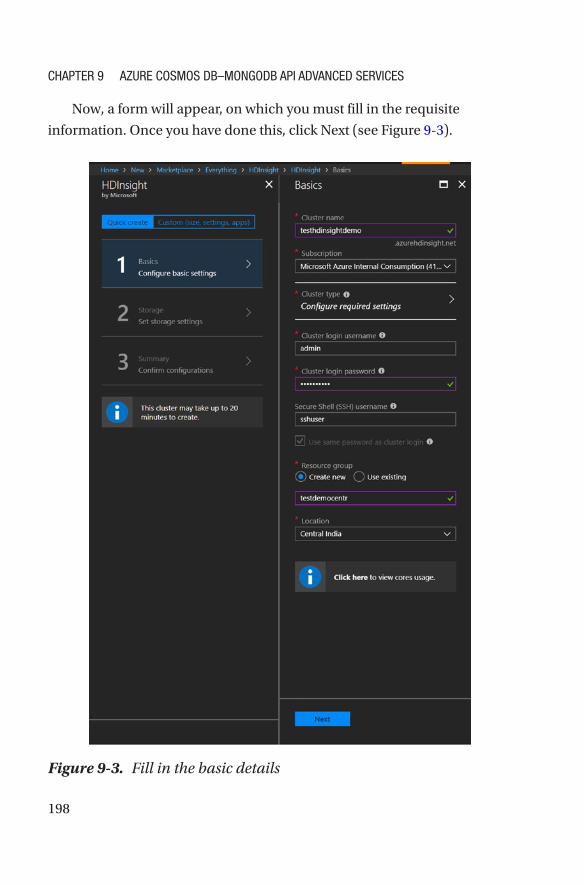
198
Now, a form will appear, on which you must fill in the requisite
information. Once you have done this, click Next (see Figure 9-3).
Figure 9-3. Fill in the basic details
Chapter 9 azure Cosmos DB–mongoDB apI aDvanCeD servICes
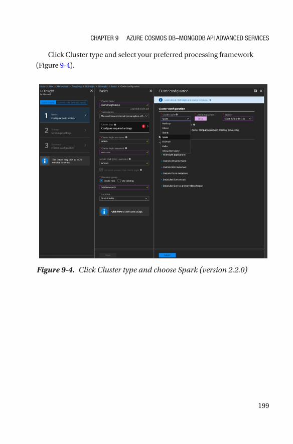
199
Click Cluster type and select your preferred processing framework
(Figure 9-4).
Figure 9-4. Click Cluster type and choose Spark (version 2.2.0)
Chapter 9 azure Cosmos DB–mongoDB apI aDvanCeD servICes
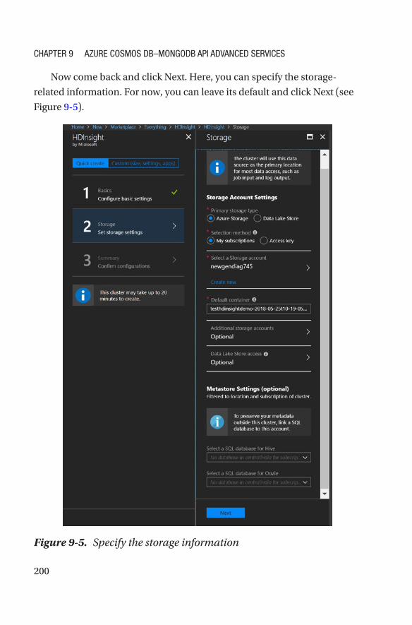
200
Now come back and click Next. Here, you can specify the storage-
related information. For now, you can leave its default and click Next (see
Figure 9-5).
Figure 9-5. Specify the storage information
Chapter 9 azure Cosmos DB–mongoDB apI aDvanCeD servICes
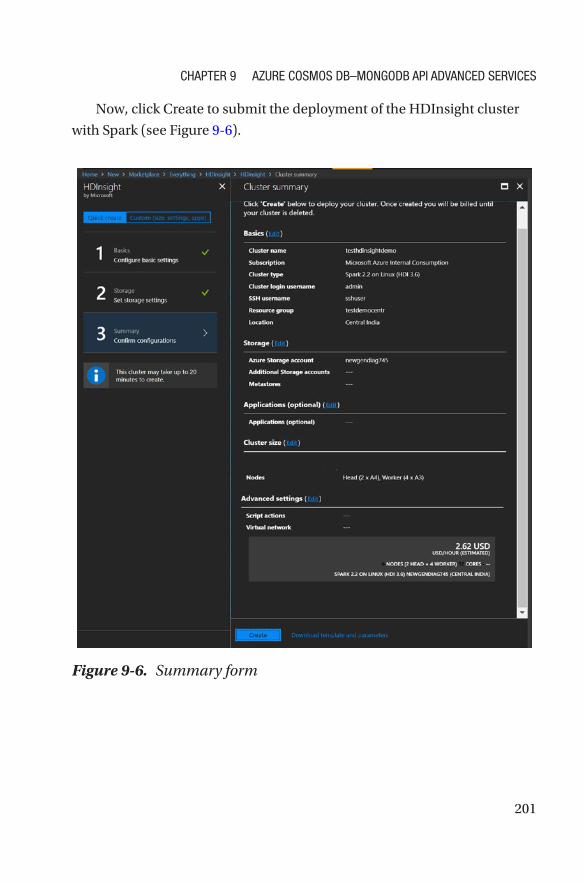
201
Now, click Create to submit the deployment of the HDInsight cluster
with Spark (see Figure 9-6).
Figure 9-6. Summary form
Chapter 9 azure Cosmos DB–mongoDB apI aDvanCeD servICes
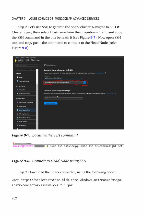
202
Step 2: Let’s use SSH to get into the Spark cluster. Navigate to SSH ➤
Cluster login, then select Hostname from the drop-down menu and copy
the SSH command in the box beneath it (see Figure 9-7). Now open SSH
tool and copy paste the command to connect to the Head Node (refer
Figure 9-8).
Step 3: Download the Spark connector, using the following code:
wget https://scaleteststore.blob.core.windows.net/mongo/mongo-
spark- connector-assembly-2.2.0.jar
Figure 9-7. Locating the SSH command
Figure 9-8. Connect to Head Node using SSH
Chapter 9 azure Cosmos DB–mongoDB apI aDvanCeD servICes

203
Step 4: Run the Spark shell command, by replacing it with your Mongo
endpoint, database, and collection details. Both input and output can be
the same.
spark-shell --conf "spark.mongodb.input.uri=mongodb://testmongo:
jsFlj8MAqCDqjaPBE2DWRhm9jRx5QfMQ3SYf9vwGxElPjZmeQKO1vbA==
@testmongo.documents.azure.com:10255/?ssl=true&replicaSet=
globaldb" --conf "spark.mongodb.output.uri=mongodb:
//testmongobook:jsF6xFsNXz6lZ3tGVjx7bErkQCzoJUzyI2lj8MAqCDqjaPBE2
DWRhm9jRx5QfMQ3SYf9vwGxElPjZmeQKO1vbA==@testmongobook.
documents.azure.com:10255/?ssl=true&replicaSet=globaldb" --conf
"spark.mongodb.input.database=db" --conf="spark.mongodb.
input.collection=eventmsgss" --conf "spark.mongodb.output.
database=db" --conf="spark.mongodb.output.collection=coll"
--jars mongo-spark-connector-assembly-2.2.0.jar
Now, after successful execution of the above code, you will get
the Scala console, which is the playground for SparkSQL. Execute the
following code:
scala> import com.mongodb.spark._
import com.mongodb.spark._
scala> import org.bson.Document
import org.bson.Document
scala> val rdd = MongoSpark.load(sc)
Now, let’s execute a few aggregate queries (see Listings 9-8 and 9-9).
Listing 9-8. Counting the Number of Records on the Basis of the Filter
scala> val agg = rdd.withPipeline(Seq(Document.parse("{ $match:
{ DeviceId : { $eq : 1004 } } }")))
scala> println(agg.count)
Chapter 9 azure Cosmos DB–mongoDB apI aDvanCeD servICes

204
Let’s see another example.
Listing 9-9. Grouping by SensorId and Counting the Values
val agg = rdd.withPipeline(Seq(Document.parse("{ $group: { _id
: '$SensorId', total:{$sum:1} } } ")))
Now, you can run all your aggregate queries more efficiently. You can
export the result to another collection of Azure Cosmos DB, which will
help you to analyze all the data and aggregate it offline. This aggregated
collection can then be used to showcase the result over the UI quickly.
ConclusionYou now have reviewed most of the Azure Cosmos DB–Mongo DB API
features and functionalities. The protocol support keeps the migration
path seamless and the learning curve minimal. In a single Azure Cosmos
DB instance, you get high availability for each partition and built-in
disaster recovery, if you configure the minimum of one geo-replication.
Also, you get the comprehensive SLAs for consistency, availability, latency,
and throughput, which can be a very costly affair to set up by yourself. This
will help you to make your application highly performant and available
throughout the year, with the least possible latency. All of this will increase
the user experience of your application. Considering these facts, it is a no-
brainer to select Azure Cosmos DB to upscale your application and add the
featured architecture tools without much hassle.
Note the azure Cosmos DB–mongoDB apI is limited by features that do not exist in mongoDB, e.g., stored procedure, functions, change feeds, etc. however, I am hopeful that all those features will soon be part of this apI.
Chapter 9 azure Cosmos DB–mongoDB apI aDvanCeD servICes
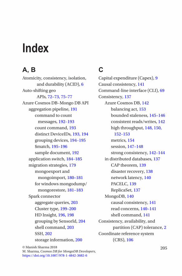
205© Manish Sharma 2018 M. Sharma, Cosmos DB for MongoDB Developers, https://doi.org/10.1007/978-1-4842-3682-6
Index
A, BAtomicity, consistency, isolation,
and durability (ACID), 6Auto-shifting geo
APIs, 72–73, 75–77Azure Cosmos DB–Mongo DB API
aggregation pipeline, 191command to count
messages, 192–193count command, 193distinct DeviceIDs, 193, 194grouping devices, 194–195$match, 195–196sample document, 192
application switch, 184–185migration strategies, 179
mongoexport and mongoimport, 180–181
for windows mongodump/mongorestore, 181–183
Spark connectoraggregate queries, 203Cluster type, 199–200HD Insight, 196, 198grouping by SensorId, 204shell command, 203SSH, 202storage information, 200
CCapital expenditure (Capex), 9Causal consistency, 141Command-line interface (CLI), 69Consistency, 137
Azure Cosmos DB, 142balancing act, 153bounded staleness, 145–146consistent reads/writes, 142high throughput, 148, 150,
152–153metrics, 154session, 147–148strong consistency, 142–144
in distributed databases, 137CAP theorem, 139disaster recovery, 138network latency, 140PACELC, 139ReplicaSet, 137
MongoDB, 140causal consistency, 141read concerns, 140–141shell command, 141
Consistency, availability, and partition (CAP) tolerance, 2
Coordinate reference system (CRS), 106
206
Cosmos DB, 11consistency, 78–79
bounded staleness, 51consistent prefix, 52eventual, 53–54session, 51strong, 50
data model, 12elastic scale, 49
storage, 49throughput, 49
geo-replication, 25aspects to consider, 28availability, 30consistency, 30latency, 29multi-geo deployment, 27reliability, 31throughput, 30
global distribution, 78–79performance, 54–55protocol support and
multimodal APICassandra API, 48Graph API, 41, 43, 45, 47–48MongoDB API, 38–40SQL (DocumentDB) API,
34–37table storage API, 32, 34
provisioning, 13–14API, 15collection ID, 19database ID, 19
Data Explorer, 19, 23enable geo-redundancy, 16ID, 15input from, 18JSON document, 22location, 16MongoDB Shell, 24pin to dashboard, 16resource group, 16shared key, 20storage capacity, 20subscription, 15throughput, 20unique key, 21
SLA, see Service level agreement (SLA)
D, E, FDatabase availability (DA), 62Disaster recovery (DR), 66, 138
GGeoJSON, 88Geo-replication, 25, 67–71
aspects to consider, 28availability, 30consistency, 30latency, 29multi-geo deployment, 27reliability, 31throughput, 30
Index
207
HHigh throughput, consistency
consistent prefix, 149–150eventual consistency, 150–151
I, J, K, LIndexing, 81
Azure Cosmos DB, 93array indexes, 96–97scale and settings page, 94–95sparse indexes, 97TTL indexes, 95–96unique indexes, 97–98
customconfiguration, 98data types, 108geospatial indexes, 105, 107hash indexes, 105modes, 99–101, 103paths, 104precision, 108range indexes, 105
in MongoDB, 81compound index, 87geospatial index, 88–89, 91hashed index, 93multikey index, 88single field index, 82–83,
85–86text index, 91–92
Infrastructure as a service (IaaS), 9
MMigration strategies, 179
application switch, 184–185
mongoexport and mongoimport, 180–181
for windows mongodump/mongorestore, 181–183
MongoDB replication, 62arbiter nodes, 64–66data-bearing
nodes, 62–64Multi-homing API, 30
NNoSQL, 2
atomicity, 6availability, 7–8and cloud, 8
IaaS, 9PaaS, 9SaaS, 10
columnar, 3consistency, 6–8document, 3–4durability, 6graph, 4–5isolation, 6key-value pair, 2–3partition
tolerance, 7–8
Index
208
OOnline transaction processing
(OLTP), 1Operating expenses (Opex), 9Optimizations, 122–126, 186–188
P, QPACELC, 7Partitioning, 113
DeviceID, 118–119DeviceID and Day, 119–120find statement, 120fixed collection, 114geo-replication, 121JSON structure of sensor
data, 117TTL limit, 121unlimited collection, 115
Partition keys, 126evaluating field to be
potential, 127message structure, 127selection, 128–129, 131, 133–135use case, 126
Platform as a service (PaaS), 9Properties graph, 41
RRelational database management
systems (RDBMSs), 2, 109Request units (RUs), 155–156
allocation, 156, 158–159calculation, 159–164data consistency, 168–170document size and
complexity, 164–165, 167indexing, 171–173, 175–176query patterns, 176–177
Rollback, 6
SService level agreement (SLA)
availability, 55–56consistency, 58latency, 59throughput, 56–57
Sharding, 109–110advantages, 113components, 110shardKey, 111
hashed key, 111–112range key, 111zones, 112–113
Sizingparameters, 155RU (see Request units (RUs))
Software as a service (SaaS), 9Spark connector
aggregate queries, 203Cluster type, 199–200HD Insight, 196, 198grouping by SensorId, 204shell command, 203
Index
209
SSH, 202storage information, 200
SQL (DocumentDB) API, 34FROM clause, 35ORDER BY clause, 36query example, 36–37SELECT clause, 35structure of query, 34
WHERE clause, 35Standby mode, 63
T, U, V, W, X, Y, ZTime-to-live (TTL)
indexes, 95–96
limit, 121
Index