Embed Size (px)
Citation preview

Clemson UniversityTigerPrints
All Theses Theses
12-2013
COST AND EMBODIED ENERGYOPTIMIZATION OF RECTANGULARREINFORCED CONCRETE BEAMSAlexander KosloskiClemson University, [email protected]
Follow this and additional works at: https://tigerprints.clemson.edu/all_theses
Part of the Civil Engineering Commons
This Thesis is brought to you for free and open access by the Theses at TigerPrints. It has been accepted for inclusion in All Theses by an authorizedadministrator of TigerPrints. For more information, please contact [email protected].
Recommended CitationKosloski, Alexander, "COST AND EMBODIED ENERGY OPTIMIZATION OF RECTANGULAR REINFORCED CONCRETEBEAMS" (2013). All Theses. 1776.https://tigerprints.clemson.edu/all_theses/1776

COST AND EMBODIED ENERGY OPTIMIZATION OF RECTANGULAR REINFORCED CONCRETE BEAMS
A Thesis Presented to
the Graduate School of Clemson University
In Partial Fulfillment of the Requirements for the Degree
Master of Science Civil Engineering
by Alexander Lawrence Kosloski
December 2013
Accepted by: Dr. Brandon Ross, Committee Chair
Dr. Leidy Klotz Dr. Weichiang Pang

ii
ABSTRACT
Concrete has a large environmental footprint so it is desirable to find ways to
efficiently design structural members. Engineers can exercise their abilities early on in
the design phase of construction projects to reduce the environmental footprint by
minimizing the amount of materials required. One way to achieve these results is to
optimize the design of structural concrete.
In this study, simple-span rectangular reinforced concrete (RC) beams with a
range of different bending moments were analyzed. The primary goal was to combine life
cycle analysis (LCA), numerical optimization, and reinforced concrete mechanics to
create a framework for designing efficient RC beams. In particular, the method was
developed to quantitatively compare the environmental preferability of RC materials with
different properties, such as high-strength reinforcement, high-strength concrete, and
lightweight (LW) concrete. The method utilizes ratios of unit cost and/or unit embodied
energy. This approach makes the method more general, and facilitates application of the
method to a wide variety of circumstances. In addition to guiding material selection, the
method also provides designers a means for quickly selecting near optimum cross-section
properties.
Trade-offs between optimum economic cost and optimum environmental footprint
were also evaluated through multiobjective optimization. The results showed that cost-
optimized beams have up to 10% more embodied energy than do energy-optimized
beams but are up to 5% cheaper than energy-optimized beams.

iii
The products of this thesis will be useful in rationally selecting materials and
designing efficient beams in terms of cost and energy.

iv
DEDICATION
I would like to dedicate this thesis to my parents, Larry and Evelyn, and the rest
of my family, Claire and Alex. I hold my parents in high esteem, for they have loved and
supported me through every single beat. I take pride in this work, knowing that they, too,
are proud of my accomplishments. Claire and Alex are my best friends and I am so lucky
to have them in my life. None of what I’ve achieved would feel as momentous were it not
for these people.

v
ACKNOWLEDGMENTS
First, I would like to thank my advisor, Dr. Brandon Ross, who is the creative
mind behind the foundation of this research. He presented the topic to me and gave me
the opportunity to work with him. Throughout the last year, he has given me all the help I
have needed and has provided me with a new understanding of civil engineering through
a structural and a sustainable point of view. Without his expertise and deep knowledge of
reinforced concrete, I could not have completed this research. I would also like to thank
Dr. Leidy Klotz and Dr. Weichiang Pang for being a part of my committee. Their
suggestions have helped refine my research by offering new perspectives, creating a more
well-rounded product.
I would like to thank two fellow graduate students whose assistance should not go
unnoticed. Michael Willis, another student of Dr. Ross, helped review my thesis and gave
some very good advice. Abby Liu, an expert in MATLAB, answered any questions I had
in regard to coding as well as general formatting in MS Word.
Lastly, I want to thank my mother; as an English teacher, she had some helpful
tips in terms of grammar and syntax, making my paper flow more easily. Everyone
played a key role in shaping my thesis and giving me the resources I needed to enhance
the final result.

vi
TABLE OF CONTENTS
Page
TITLE PAGE .................................................................................................................... i ABSTRACT ..................................................................................................................... ii DEDICATION ................................................................................................................ iv ACKNOWLEDGMENTS ............................................................................................... v LIST OF TABLES ........................................................................................................ viii LIST OF FIGURES ........................................................................................................ ix CHAPTER I. INTRODUCTION AND BACKGROUND .................................................. 1 Introduction .............................................................................................. 1 Research Objectives ................................................................................. 2 Reinforced Concrete Materials ................................................................ 3 Optimization Basics ................................................................................. 8 Green Concrete Strategies ........................................................................ 9 II. REVIEW OF OPTIMIZATION STUDIES ................................................. 13 Introduction ............................................................................................ 13 Optimization Methods ........................................................................... 14 Previous Works ...................................................................................... 16 Distinctions of Current Study ................................................................ 27 Literature Review Summary .................................................................. 29
III. OPTIMIZATION OF REINFORCED CONCRETE BEAMS METHODOLOGY ................................................................................ 31
Overview ................................................................................................ 31 Nomenclature ......................................................................................... 31 Problem Statement ................................................................................. 34 Computer Programs ............................................................................... 35 Design Variables .................................................................................... 37 Parameters .............................................................................................. 41

vii
Table of Contents (Continued)
Page Constraints ............................................................................................. 44 Code and Methods ................................................................................. 45 IV. PARAMETRIC STUDIES WITH EMBODIED ENERGY OPTIMIZED .......................................................................................... 57 Overview ................................................................................................ 57 Effects of Parameters on Problem Set-Up ............................................. 73 Parametric Studies ................................................................................. 79 V. PARAMETRIC STUDIES WITH COST OPTIMIZED ............................. 99 Overview ................................................................................................ 99 Parametric Studies ............................................................................... 102 VI. SUMMARY AND CONCLUSIONS ........................................................ 115 Summary and Conclusions .................................................................. 115 Recommendations for Future Work ..................................................... 117 APPENDICES ............................................................................................................. 119 A: Supplementary Studies with Embodied Energy Optimized ....................... 120 B: Supplementary Studies with Cost Optimized ............................................ 125 C: Extended Bibliography .............................................................................. 127 REFERENCES ............................................................................................................ 133
viii
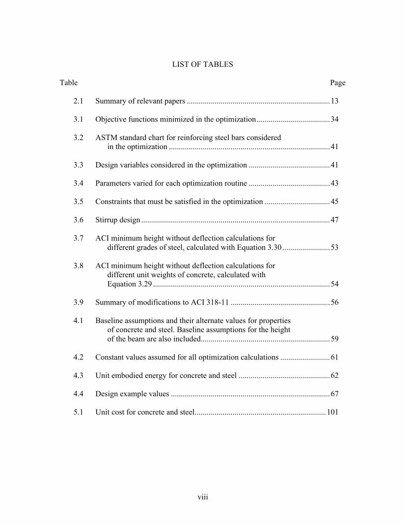
LIST OF TABLES
Table Page 2.1 Summary of relevant papers ........................................................................ 13 3.1 Objective functions minimized in the optimization ..................................... 34 3.2 ASTM standard chart for reinforcing steel bars considered in the optimization ................................................................................. 41 3.3 Design variables considered in the optimization ......................................... 41 3.4 Parameters varied for each optimization routine ......................................... 43 3.5 Constraints that must be satisfied in the optimization ................................. 45 3.6 Stirrup design ............................................................................................... 47 3.7 ACI minimum height without deflection calculations for different grades of steel, calculated with
Equation 3.30 ........................ 53
3.8 ACI minimum height without deflection calculations for different unit weights of concrete, calculated with
Equation 3.29 ......................................................................................... 54 3.9 Summary of modifications to ACI 318-11 .................................................. 56 4.1 Baseline assumptions and their alternate values for properties of concrete and steel. Baseline assumptions for the height of the beam are also included ................................................................. 59 4.2 Constant values assumed for all optimization calculations ......................... 61 4.3 Unit embodied energy for concrete and steel .............................................. 62 4.4 Design example values ................................................................................ 67 5.1 Unit cost for concrete and steel .................................................................. 101

ix
LIST OF FIGURES
Figure Page 2.1 (a) Typical curve of cost optimum steel ratio, (b) Simply supported beam, f’c = ksi and fy = 50 ksi ............................................... 18 2.2 Total costs for different breadths for cross sections exposed to 500 kN-m ........................................................................................... 19 2.3 Total costs for different breadths for cross sections exposed to 700 kN-m ........................................................................................... 20 2.4 Variation in percentage difference in cost and embodied energy with R, b equals 400 mm ........................................................... 21
2.5 Relation between CO2 emissions and cost ................................................... 24
2.6 (a) Dependence upon the cost ratio of the percentage of total cost and CO2 emissions for the cost-optimized frame and the CO2-optimized frame, (b) Dependence upon the CO2 ratio of the percentage of total cost and
CO2 emissions for the cost-optimized frame and the CO2-optimized frame, (c), Dependence upon concrete compressive strength of the percentage of total cost and CO2 emissions for the cost-optimized frame and the CO2-optimized frame ............................................................................. 27
3.1 Typical cross-section of a rectangular reinforced concrete beam ....................................................................................................... 35 3.2 All configurations of longitudinal reinforcement utilized in the optimization of reinforcement concrete beams, categorized by number of rebar ............................................................. 39 3.3 Beam without stirrups .................................................................................. 48
3.4 Stirrup spacing for ............................................................... 49
3.5 Stirrup spacing for ......................................................................... 50
φVc2<Vu ≤ φVc
Vu > φVc

x
List of Figures (Continued) Figure Page 4.1 Example figure describing baseline and alternative values for parameters ........................................................................................ 60 4.2 Example figure comparing the embodied energy ratios for 60 ksi and 75 ksi steel reinforcement ..................................................... 64 4.3 Design example of simply supported beam exposed to distributed load ....................................................................................... 67 4.4 Design example comparing the embodied energy ratios for 60 ksi and 75 ksi steel reinforcement ..................................................... 68 4.5 Design example demonstrating the effects of the unit embodied energy ratio of steel on the aspect ratio ................................................. 69 4.6 Design example demonstrating the effects of the unit embodied energy ratio of steel on the reinforcement ratio ..................................... 70 4.7 Design example demonstrating the effects of the unit embodied energy ratio of steel on the span-to-depth ratio ..................................... 70 4.8 Cross-section of design example, drawn to scale ........................................ 71 4.9 Recommended reinforcement ratio comparisons to Alreshaid et al. (2004) for 60 ksi steel reinforcement ............................................ 72 4.10 Total embodied energy of the cost-optimized design divided by the total embodied energy of the embodied energy- optimized design with variable span-to-depth ratio ............................... 73 4.11 Percentage of possible solutions that are feasible for different grades of steel reinforcement ................................................................. 74 4.12 Percentage of possible solutions that are feasible for different
grades of concrete .................................................................................. 75 4.13 Percentage of possible solutions that are feasible for different unit weights of concrete ......................................................................... 75

xi
List of Figures (Continued) Figure Page 4.14 Contribution of 60 ksi shear reinforcement to the total embodied energy of the beam ................................................................................. 76 4.15 Contribution of 60 ksi shear reinforcement to the total cost of the beam ............................................................................................. 76 4.16 Average number of layers of reinforcement for different grades of steel reinforcement when optimized for embodied energy ..................................................................................................... 78
4.17 Average number of layers of reinforcement for different grades of concrete when optimized for embodied energy ..................... 78
4.18 Average number of layers of reinforcement for different unit weights of concrete when optimized for embodied energy ............ 78 4.19 Comparison of embodied energy ratios for 60 ksi and 75 ksi steel reinforcement ........................................................................... 80
4.20 Comparison of embodied energy ratios for 60 ksi and 120 ksi steel reinforcement ........................................................................... 80 4.21 Aspect ratio for different grades of steel reinforcement when optimized for embodied energy ............................................................. 82 4.22 Reinforcement ratio for different grades of steel reinforcement when optimized for embodied energy .................................................... 84 4.23 Recommended reinforcement ratio for different grades of steel reinforcement when optimized for embodied energy .................... 84
4.24 Span-to-depth ratio for different grades of steel reinforcement when optimized for embodied energy .................................................... 85
4.25 Aspect ratio for different grades of steel reinforcement when optimized for embodied energy ............................................................. 86
4.26 Reinforcement ratio for different grades of steel reinforcement when optimized for embodied energy .................................................... 87

xii
List of Figures (Continued) Figure Page 4.27 Recommended reinforcement ratio for different grades of steel reinforcement when optimized for embodied energy .................... 87 4.28 Span-to-depth ratio for different grades of steel reinforcement when optimized for embodied energy .................................................... 88 4.29 Comparison of embodied energy ratios for 4,350 psi and 6,000 psi concrete .................................................................................. 89 4.30 Comparison of embodied energy ratios for 4,350 psi and 10,000 psi concrete ................................................................................ 89
4.31 Aspect ratio for different grades of concrete when optimized for embodied energy .............................................................................. 91 4.32 Reinforcement ratio for different grades of concrete when optimized for embodied energy ............................................................. 92 4.33 Recommended reinforcement ratio for different grades of concrete when optimized for embodied energy ..................................... 92 4.34 Span-to-depth ratio for different grades of concrete when optimized for embodied energy .............................................................................. 93 4.35 Comparison of embodied energy ratios for 145 pcf and 90 pcf concrete ............................................................................................ 95 4.36 Comparison of embodied energy ratios for 145 pcf and 115 pcf concrete ............................................................................................ 95 4.37 Aspect ratio for different unit weights of concrete when optimized for embodied energy ............................................................. 96 4.38 Reinforcement ratio for different unit weights of concrete when optimized for embodied energy .................................................... 97 4.39 Recommended reinforcement ratio for different unit weights of concrete when optimized for embodied energy ................................. 97

xiii
List of Figures (Continued) Figure Page 4.40 Span-to-depth ratio for different unit weights of concrete when optimized for embodied energy .................................................... 98 5.1 Comparison of cost ratios for 60 ksi and 120 ksi steel reinforcement ....................................................................................... 103 5.2 Aspect ratio for different grades of steel reinforcement when optimized for cost ................................................................................ 104
5.3 Reinforcement ratio for different grades of steel reinforcement when optimized for cost ....................................................................... 104
5.4 Recommended reinforcement ratio for different grades of steel reinforcement when optimized for cost ....................................... 105
5.5 Span-to-depth ratio for different grades of steel reinforcement when optimized for cost ....................................................................... 105
5.6 Comparison of cost ratios for 4,350 psi and 10,000 psi concrete ................................................................................................ 106
5.7 Aspect ratio for different grades of concrete when optimized for cost ................................................................................................. 107 5.8 Reinforcement ratio for different grades of concrete when optimized for cost ................................................................................ 107 5.9 Recommended reinforcement ratio for different grades of concrete when optimized for cost ........................................................ 108 5.10 Span-to-depth ratio for different grades of concrete when optimized for cost ................................................................................ 108 5.11 Comparison of cost ratios for 145 pcf and 115 pcf concrete ..................... 109 5.12 Aspect ratio for different unit weights of concrete when optimized for cost ............................................................................... 110
5.13 Reinforcement ratio for different unit weights of concrete when optimized for cost ....................................................................... 110
xiv
List of Figures (Continued) Figure Page 5.14 Recommended reinforcement ratio for different unit weights of concrete when optimized for cost .................................................... 110
5.15 Span-to-depth ratio for different unit weights of concrete when optimized for cost ....................................................................... 111
5.16 Total embodied energy of the beam when optimized for embodied energy and for cost .............................................................. 113
5.17 Total embodied energy of the cost-optimized design divided by the total embodied energy of the embodied energy-optimized design ...................................................................... 113
5.18 Total cost of the beam when optimized for embodied energy and for cost ........................................................................................... 113
5.19 Total cost of the embodied energy-optimized design divided by the total cost of the cost-optimized design ...................................... 114 A.1 Comparison of embodied energy ratios for 60 ksi and 40 ksi steel reinforcement ......................................................................... 120 A.2 Comparison of embodied energy ratios for 60 ksi and 90 ksi steel reinforcement ......................................................................... 120 A.3 Comparison of embodied energy ratios for 60 ksi and 100 ksi steel reinforcement ......................................................................... 121 A.4 Comparison of embodied energy ratios for 4,350 psi and 2,500 psi concrete ................................................................................ 121 A.5 Comparison of embodied energy ratios for 4,350 psi and 8,000 psi concrete ................................................................................ 121 A.6 Aspect ratio for different grades of concrete when optimized for embodied energy ............................................................................ 122 A.7 Reinforcement ratio for different grades of concrete when optimized for embodied energy ........................................................... 122

xv
List of Figures (Continued) Figure Page A.8 Recommended reinforcement ratio for different grades of concrete when optimized for embodied energy ................................... 122 A.9 Span-to-depth ratio for different grades of concrete when optimized for embodied energy ........................................................... 123 A.10 Comparison of embodied energy ratios for 145 pcf and 103 pcf concrete ................................................................................... 123 A.11 Aspect ratio for different unit weights of concrete when optimized for embodied energy ........................................................... 123 A.12 Reinforcement ratio for different unit weights of concrete when optimized for embodied energy .................................................. 124 A.13 Recommended reinforcement ratio for different unit weights of concrete when optimized for embodied energy ............................... 124 A.14 Span-to-depth ratio for different unit weights of concrete when optimized for embodied energy .................................................. 124 B.1 Comparison of cost ratios for 60 ksi and 40 ksi steel reinforcement ....................................................................................... 125 B.2 Comparison of cost ratios for 4,350 psi and 2,500 psi concrete ................ 125 B.3 Comparison of cost ratios for 145 pcf and 90 pcf concrete ....................... 126

1
CHAPTER ONE
INTRODUCTION AND BACKGROUND
1.1 Introduction
Construction projects require costly investments of time and money. In the last
decade, environmental costs of construction have also become a primary concern. One
example of an environmental cost is carbon dioxide and other greenhouse gases emitted
into the atmosphere as a result of construction activities. Therefore, engineers exercise
their abilities early on in the design phase of construction projects to help reduce the cost
and carbon footprint by lessening the amount of materials required. One way to achieve
these results is to optimize the design of structural members.
Because concrete is the most commonly used construction material on the planet,
and with the cement industry responsible for 5% of the world’s carbon dioxide emissions
(Worrell, 2001), the current research focuses on the optimization of reinforced concrete
(RC) members. By optimizing these RC structures, engineers can scale down the volume
of concrete and/or steel used in a structure, consequently lowering the discharge of
carbon dioxide emissions, as well as other environmental costs, and the economic costs
associated with construction. This study will focus on optimizing RC beams for
embodied energy, which is defined as the quantity of energy needed to develop and
manufacture a product, as if that energy were manifested within the product itself.
Different techniques have been utilized in this research to conduct optimization
on RC members; these methods are discussed in the next chapter. Each method defines a
set number of design variables that are modified within the optimization process, such as

2
the height and width of the member and the area of steel reinforcement placed within the
member. These design variables are modified in a fashion that would minimize the
objective function; examples of such objective functions are the total cost of the structure
and the energy consumed by all the materials and processes necessary to produce the
structure. Constraints are also applied to ensure that the optimized structure satisfies code
while prevailing as a dependable and durable structural component; these constraints can
be the flexural or shear capacity of the member but are not limited to these two principles
of structural engineering.
1.2 Research Objectives
While previous research has studied optimization of multiple RC elements, this
research is being performed specifically on RC beams, optimizing them for economic and
environmental costs. The overall purpose is to combine life cycle analysis (LCA),
optimization techniques, and reinforced concrete mechanics to create a quantitative
framework for designing sustainable RC structures. Specific goals include the creation of
a methodology for rationally comparing the environmental preferability of different RC
materials and the creation of a procedure for designing environmentally optimum RC
beams.
To accomplish these goals, various parametric studies have been developed to
evaluate how high-performance materials can be used in practice by designers to improve
the efficiency of RC beams. These parametric studies utilized optimization methods and
considered a wide range of design variables, reinforcement configurations, and material
properties.

3
To assist designers in the design of optimized members, the parametric studies
have been shaped so that different materials can be selected based on environmental or
cost efficiency. After it has been established which material is best suited for their
application, the designer can utilize results of supplementary parametric studies to
determine the optimal cross-sectional design.
While embodied energy is the only environmental metric considered in this thesis,
there are many other metrics that can be applied to the impact assessment of reinforced
concrete. Other metrics used in the life-cycle inventory of construction materials include
mineral depletion, land use, and human toxicity. Human toxicity is a concern when
dealing with chemical additives, such as fly ash.
1.3 Reinforced Concrete Materials
1.3.1 Concrete
Concrete consists of four primary ingredients: cement, coarse aggregate, fine
aggregate, and water. Additives are also typically included in the mix to improve
properties of the concrete, such as durability, workability, or set-time (Mehta &
Monteiro, 1993). A list of definitions has been given for commonly used materials in
concrete as well as additives and replacements to enhance its functionality.
Cementitious Materials. Cement is a powdery material that has cementing value
when used in concrete either by itself, such as Portland cement, or in combination with
products such as fly ash, silica fume, and/or ground granulated blast-furnace slag (ACI
Committee 318, 2011).

4
Aggregate. Aggregate is a granular material, such as sand, gravel, crushed stone,
and iron blast-furnace slag, used with a cementing medium to form a hydraulic cement
concrete or mortar (ACI Committee 318, 2011). Typical raw materials that are regularly
used as aggregate are quartz, basalt, granite, marble, and limestone. The majority of the
contents within a concrete mix are aggregate while that aggregate’s physical properties
significantly influence the “workability, durability, strength, weight, and shrinkage of the
concrete” (The Concrete Countertop Institute, 2006).
Aggregate is broken up into two primary categories: coarse aggregate and fine
aggregate. Coarse aggregate is larger than ¼ inch while fine aggregate is smaller than ¼
inch. Fine aggregate is used to fill in gaps between larger particles, thus minimizing the
demand for cement paste in the mix; this also mitigates any shrinking within the concrete
(TCCI, 2006).
While normal weight (NW) aggregate is used to produce NW concrete for general
purposes, lightweight (LW) aggregate is an alternative to reduce the self-weight of the
beam. LW aggregate is typically expanded shale, clay, and slate materials, which have
been ignited in a rotary kiln to give them a porous consistency. These aggregates are used
to produce a LW concrete (National Ready Mixed Concrete Association, 2003), which
has a unit weight between 90 pcf and 115 pcf. NW concrete has a greater unit weight,
between 135 pcf and 160 pcf (ACI Committee 318, 2011).
Recycled materials have also been given attention to reduce environmental and
economic costs. One is recycled glass aggregate (RGA), which is cullet milled from
recycled glass products and used as aggregate replacement; an alkali-silica reaction
5
(ASR) occurs between the cement and glass (when particles are large enough to be
considered aggregate) that may cause degradation in the concrete over time. Another
recycled material is recycled concrete aggregate (RCA), which is concrete from
demolition and renovation projects that is crushed and stripped of all reinforcement so it
can be used as aggregate replacement.
Water. Water is added to concrete mixes to activate the cement and to create a
mix that is more workable; hydraulic cements require water to harden.
Admixtures. Admixtures are materials other than water, aggregate, or hydraulic
cement, used as an ingredient of concrete and added to concrete before or during its
mixing to modify its properties (ACI Committee 318, 2011). Seven classic admixtures
are listed and defined:
1. A set-retarding admixture impedes the chemical reaction that occurs when the
concrete begins to harden, or set. In doing this, more time is given to install
concrete, especially in hot climates, which tend to expedite the setting process
(Mehta & Monteiro, 1993).
2. Accelerators refer to two properties: high early strength and increased setting
time (Mehta & Monteiro, 1993).
3. Air-entrainment improves the durability of the concrete exposed to extreme
temperatures; extreme temperatures induce a cycle of freezing and thawing that
causes the concrete to expand and contract and eventually form cracks. Air-
entrainment also enhances the workability of the concrete (Mehta & Monteiro,
1993).

6
4. Water-Reducers are used to acquire a certain strength while expending less
cement by lowering the water-cement ratio required to achieve an acceptable
slump (Mehta & Monteiro, 1993).
5. Shrinkage-reducing admixtures reduce short- and long-term drying shrinkage
that results in the degradation of the concrete due to cracking (Rodriguez).
6. Superplasticizers increase the workability of the concrete while yielding a
concrete with a high slump; this allows for the placement of concrete in densely
reinforced structures or areas where sufficient consolidation is not easily
attainable (Rodriguez).
7. Corrosion-inhibiting admixtures hinder the effects of corrosion on reinforcing
steel present in concrete (Rodriguez).
Supplementary Cementitious Materials (SCM). SCMs are used to replace the
Portland cement to reduce the economic and environmental costs. The four most common
are fly ash (FA), ground granulated blast-furnace slag (GGBS), silica fume (SF) and glass
powder (GLP). FA is a by-product of the combustion of coal during the generation of
electricity. Before GGBS can be used as a cement replacement in concrete, blast-furnace
slag, a by-product of the production of iron ore, must be ground into a powder (Ali &
Fiaz, 2009). SF is a by-product of silicon metal and ferrosilicon alloy production (Mehta
& Monteiro, 1993). GLP is pulverized glass cullet but does not experience the same
degradation found in concrete with RGA; this is due to the pulverizing of glass into a fine
powder, which mitigates any effects initiated by ASR.

7
Grades. The grade of concrete refers to the compressive strength (f’c) of the
concrete. Different grades of concrete are used in different conditions where higher
strength may be required. By including admixtures and adjusting the proportions of
water, cement, and aggregate within the concrete mix, increased compressive strength
can be achieved. High-strength concrete is described as having a compressive strength
greater than 6,000 psi (ACI Committee 363, 1992).
1.3.2 Steel (Reinforcement)
While concrete is strong in compression, it is weak in tension. It is also brittle and
therefore liable to break without warning. As a simply supported RC beam deflects, it
forms a U-shape with the bottom in tension. Cracks begin to develop at the bottom, so
longitudinal reinforcement is placed on the tension side of the beam to carry forces as the
concrete cracks, creating a hybrid between concrete and steel that is strong in both
compression and tension, as well as ductile. Different coatings are also applied to steel
reinforcement to protect it against corrosion. A list of definitions has been given below
for common variations in steel reinforcement.
Recycled Materials. Steel reinforcement can either be virgin or recycled. Virgin
steel is pure or has never been recycled. However, reinforcement used today is at least
97% recycled material from other steel products (Concrete Joint Sustainability Initiative,
2009); recycled steel reinforcement has a unit embodied-energy coefficient that is
typically around 8.9 MJ/kg while a typical unit embodied-energy coefficient of virgin
steel reinforcement is 32.0 MJ/kg, more than three times that of recycled material (Table
of embodied energy coefficients, 2007).

8
Types/Coatings. Most vendors that sell steel reinforcement offer an assortment
with distinct practical characteristics. Black reinforcement is uncoated steel that is cheap
but subject to corrosion. Epoxy-coated reinforcement (ECR) bears a membrane that has
been applied to defend it against corrosive elements in marine and other harsh
environments. Galvanized reinforcement, on the other hand, is coated with several layers
of zinc oxide to protect it against corrosion. The zinc forgoes oxidation to spare the
reinforcement of any degradation. Stainless steel is a more expensive option but is very
resistant against corrosion; this element can either be applied as a coating or adopted as
an alternative material for the composition of the reinforcement (Johnson, 2010).
Grades. The grade of steel refers to the yield strength (fy) of the steel
reinforcement. 60 ksi steel is the most common grade of reinforcement, but other yield
strengths (40, 75, 90, 100, and 120 ksi) are also available. High yield strength steel can be
used to reduce a structure’s demand for reinforcement and therefore cut back on the
congestion in each structural member, as well as the labor required to install the
reinforcement.
1.4 Optimization Basics
Optimization programs are divided into two functions: the objective function and
the constraint function; design variables and other parameters are then defined for each of
these actions. The objective function is the value being minimized in the optimization;
common examples are cost, embodied energy, and CO2 emissions. Constraints are the
maximum and minimum values, calculated based on standard engineering code, that each
set of design variables must satisfy in order to be a feasible solution. Design variables are

9
adjusted to optimize the objective function and must be included in the calculation of that
objective function. Other parameters not included in the direct design of the structure are
kept constant during each optimization routine, such as beam span and cost and embodied
energy of materials.
There is a standard form for writing optimization problems as algorithms. The
objective function and constraints are written as two separate functions with every
variable previously defined. All constraints must be set to zero; the larger value is
subtracted from the smaller value. For example, if the width of the beam must be greater
than a minimum value, bmin, then the standard form would be bmin – b = 0. In discrete
optimization problems, each design variable consists of a range of integers that are
arranged into a vector. These values are then mapped through the constraint function and
the objective function. Other parameters are defined as constants for each optimization.
1.5 Green Concrete Strategies
A number of green strategies have been adopted in the production of reinforced
concrete to create more efficient members, reducing the amount of raw materials that the
structure demands. One strategy is to utilize recycled materials, which are by-products or
waste materials and are used in reinforced concrete to reduce the cost and/or carbon
footprint of the structure. Recycled materials help to reduce the carbon footprint
otherwise caused by virgin materials, such as Portland cement and steel.
Industrial by-products are commonly used as cement replacements in concrete to
enhance its performance as well as reduce the environmental footprint. Fly ash, a by-
product of coal during the combustion of electricity, can act as a partial replacement for

10
Portland cement. Ground granulated blast-furnace slag and glass powder are two more
alternatives to Portland cement that possess a much lower unit embodied-energy
coefficient than the cement, especially if classified as wastes.
Substituting some of the components within reinforced concrete with high-
strength or LW materials may have greater unit costs, but they can also be used to
minimize the materials necessary to satisfy the flexural capacity of the member, thus
reducing the overall cost. One product that is becoming more popular in the U.S. is
MMFX2 steel reinforcement. These bars are uncoated, but they possess unique chemical
and mechanical properties that enhance their performance as reinforcing steel. Although
most steel forfeits brittleness in the name of strength, MMFX2 steel actually manages to
be both stronger and tougher. According to MMFX Technologies Corporation (2012),
“Structural systems reinforced with MMFX2 rebars have been shown to achieve design
service lives in excess of 75 years.” As high-strength and corrosion-resistant steel,
MMFX2 steel reinforcement meets or surpasses the specifications of ASTM A615 Grades
75 and 80.
In the North American market, #3 through #11, #14, and #18 standard bars are
sold. Forty- and sixty-foot bundles are available, as well as custom-mill-cut lengths of up
to 72 ft for all sizes and 80 ft for #11, #14, and #18 bars. MMFX vendors provide two
grades of steel: Grade 100 and Grade 120. Both of these are certified and are suitable for
construction of reinforced concrete.
MMFX2’s excellent resistance to corrosion has also proven to reduce the cost of
repairs. While initial costs are sometimes greater than initial costs of conventional

11
reinforcement, the long-term costs are greatly reduced. Therefore, high-strength steel can
be a cost-effective alternative while also reducing construction time by cutting down on
the demand for steel (MMFX Technologies Corporation, 2012).
LW concrete is another product that has been promoted to reduce the
environmental costs of RC structures. LW concrete is achieved by using LW aggregate,
which has a more porous consistency than does NW aggregate.
LW concrete also tends to be more costly (National Ready Mixed Concrete
Association, 2003), and while it does not increase the strength of the material, it reduces
the self-weight of the beam, producing a smaller moment throughout the specimen. This
helps lessen the volume of the concrete or steel required to support a heavier beam. LW
concrete may affect lower load demands due to its low unit weight, but that is only one of
several advantages it enjoys. Lighter weight means a larger number of RC members per
truck, especially when weight limits on roads are a factor. Fewer truck loads ensures
lower transportation costs and less CO2 emissions.
With LW aggregate’s ability to absorb higher volumes of water, NW aggregate
can be substituted with LW aggregate when concrete is designed with low water-to-
cement ratios. This “internal curing” can suppress the “self-desiccation and early-age
cracking” that high-cementitious concretes are susceptible to. LW concrete has also
proven to have a greater fire tolerance than its NW concrete equivalent due to “a
combination of lower thermal conductivity, lower coefficient of thermal expansion, and
the inherent thermal stability developed by aggregates that have been already exposed to
temperature greater than 2000 degrees Fahrenheit during pyroprocessing.”
12
When using air-entrained LW concretes, durability is not compromised.
Numerous studies regarding LW concrete’s durability have delivered positive results.
However, due to the lower aggregate stiffness that is characteristic of LW concrete, LW
concrete generally experiences a slightly larger degree of shrinkage than does NW
concrete (Holm & Ries, 2006).

13
CHAPTER TWO
REVIEW OF OPTIMIZATION STUDIES
2.1 Introduction
Optimization of reinforced concrete (RC) structures was first studied in the 1970s
by Rozvany (1970), Leroy (1974), and Chou (1977), among others, and has subsequently
been the subject of numerous technical papers and reports. Many of these works are listed
in the Extended Bibliography section of this thesis (Appendix C). Papers most relevant to
the current study are discussed in this chapter. Papers were ruled as relevant based on
common links to the current research, such as multiobjective optimization of economic
and environmental costs or parametric studies consisting of the reinforcement ratio, the
cost ratio, the compressive strength of the concrete, or the external applied moment. Key
points from these works are highlighted, and knowledge gaps are identified. The most
relevant papers and their features are summarized in Table 2.1.
Table 2.1: Summary of relevant papers.
1Width, b, is held constant for each iteration; vector of four values defined. 2Reinforcement ratio, ρ, is used in place of the area of steel, As. 3Type of steel and type of concrete are also considered design variables. C: Continuous D: Discrete BB-BC: Big bang-big crunch algorithm SA: Simulated Annealing algorithm
Year Beam Frame BB(BC SA Other Economic Environ b h As Av
Samman 1995 X X X D1 C C2 (Alreshaid 2004 X X X D D C2 (
Yeo 2011 X X X X D D C CPaya3 2008 X X X X D D D D
Paya(Zaforteza3 2009 X X X X D D D DCamp 2013 X X X X D D D (Yeo 2013 X X X X C C C (
Structure Method ObjectiveLFunctions BeamLDesignLVariables

14
2.2 Optimization Methods
Different numerical methods are available for locating optimum design solutions.
Papers discussed in this chapter used the following methods: the direct search (DS)
algorithm, the simulated annealing (SA) algorithm, and the big bang-big crunch (BB-BC)
algorithm. Another algorithm commonly used is the genetic algorithm (GA), but there are
additional algorithms, both heuristic and non-heuristic, used to perform optimization.
Unlike non-heuristic methods, “[heuristic] methods are based on the principles of natural
biological evolution” (Alqedra et al., 2011).
The process of optimization can be divided into two categories: direct and
gradient-based methods. Direct search methods use an objective function and constraints
to search for the solution while “gradient-based methods use the first and/or second-order
derivatives of the objective function and/or constraints to guide the search process”
(Alqedra et al., 2011). During the pursuit of an optimal solution, the direct search
algorithm accesses a group of points around a current point, searching for another that
possesses a lower objective function than the previous point. Such a method can only be
used for non-differentiable objective functions (Mathworks, 2013).
Heuristic methods have become prominent in the optimization of reinforced
concrete. Examples of heuristic methods commonly used are GA, SA, and more recently,
BB-BC. The primary issue among these algorithms is the conflict of “accuracy,
reliability, and computation time” (Erol & Eksin, 2006).
Using Darwin’s theory of evolution, the GA searches a design space consisting of
a population of designs. These designs, or solutions, are generated stochastically. Designs

15
are then selected at random, with better designs having a higher chance of being chosen,
echoing Darwin’s survival of the fittest. In order to converge towards the optimum point,
mutations and crossovers occur; mutations are small variations in one or more design
variables whereas crossovers occur so that individual solutions are combined to produce
new and unique solutions (Alqedra et al., 2011; Kohonen, 1999). The GA has been used
to study RC structures by Coello Coello et al. (1997), Camp et al. (2003), Govindaraj and
Ramasamy (2005), and Alqedra et al. (2011).
Much like the GA, the SA algorithm approaches the optimum solution by
modifying the existing solution using the mutation effect. However, the SA algorithm has
only one population, and therefore only one solution; thus, crossover does not occur.
These differences do not make one algorithm superior over the other but rather create
different tools that work better or worse depending upon the formation of the problem.
Each of these algorithms shares the idea that desirable solutions can be located close to
formerly established suitable points (Kohonen, 1999). The SA algorithm has been used to
study RC structures by Leps and Sejnoha (2003), Martinez et al. (2007), Paya et al.
(2008), and Paya-Zaforteza et al. (2009).
A more recent development in the realm of optimization is the BB-BC algorithm.
Inspired by the theory regarding the evolution of the universe, the BB-BC algorithm
relies on a “population-based search procedure that incorporates random variation and
selection,” similar to the GA and SA algorithms. Unlike the GA and SA algorithms, it is
comprised of two phases: the Big Bang phase and the Big Crunch phase. During the Big
Bang phase, random points are created throughout the design space, mimicking the
16
dissipation of energy; in the Big Crunch phase, those points are then condensed into a
single point expressed as a center of mass, mimicking the attraction initiated by gravity.
The center of mass is used to distribute new offspring around the known point; once the
points converge again, the center of mass is re-evaluated. This process continues through
multiple iterations until the stopping criteria are satisfied (Erol & Eksin, 2006). BB-BC
has been used to study RC structures by Camp and Akin (2012), Camp and Huq (2013),
and Camp and Assadollahi (2013).
In Erol and Eksin (2006), the BB-BC algorithm was shown to be more reliable
and efficient than the GA because the GA does not always converge to the global
optimum due to its “selective capacity of the fitness function” and because the GA has a
higher computational time. The study showed that the BB-BC method reduced the
computational time by a large margin while locating the global minimum “within the
maximum number of allowed iterations” (Erol & Eksin, 2006).
2.3 Previous Works
This section summarizes papers on the optimization of beams and frames that
relate most closely to the studies in this thesis. Each of these papers considered reinforced
concrete structures that have been optimized for minimum economic cost, minimum
environmental cost, or both.
2.3.1 RC Beams
Samman and Erbatur (1995), Alreshaid et al. (2004), and Yeo and Gabbai (2011)
optimized rectangular RC structures with a given length. While Samman and Erbatur
(1995) and Alreshaid et al. (2004) minimized economic cost exclusively, Yeo and Gabbai

17
(2011) minimized economic and environmental costs simultaneously. Each of these
papers is discussed in greater detail in the following subsections.
Samman and Erbatur (1995)
Samman and Erbatur (1995) approached the problem of RC optimization using a
systematic DS algorithm. The width of the beam was given while the height and main
reinforcement were calculated so that the nominal moment capacity constraint was
satisfied for each given width; therefore, the height and longitudinal steel reinforcement
ratio were calculated with a range of continuous values while the width was defined by a
vector of discrete variables. A set of moments ranging from 5 k-in to 500,000 k-in was
considered to demonstrate low and high loading conditions.
Rather than using fixed costs, a range of steel-to-concrete cost ratios were
computed per unit weight and used to establish trends for varying reinforcement ratios.
This is shown in Figure 2.1(b), with the cost-optimum reinforcement ratio decreasing
exponentially as the cost of the steel rises relative to the cost of concrete. A typical
relationship between cost ratio and reinforcement ratio is given in Figure 2.1(a). Each
segment of the curve is given a label (R1, R2, etc.) to signify different optimization
regions. R1 is the maximum optimal steel-ratio region, consisting of beams with a
minimum width and height; R2 is the cost-sensitive region, with beams having a greater
volume of concrete due to an increase of beam height, which is directly linked to the
reduction of the steel ratio; R3 is the intermediate constant-ratio region, and only pertains
to fixed-fixed and fixed-hinged beams; R4 is the cost-insensitive region, which
corresponds to overly designed beams. The effects produced by an array of parameters

18
were examined for notable trends. Particular parameters displayed more influence on the
reinforcement ratio than others: end conditions and material costs had substantial effects,
applied loads and yield strength had considerable effects, and concrete strength and beam
width had negligible effects.
Figure 2.1: (a) Typical curve of cost optimum steel ratios, (b) Simply supported beam, f’c = 3 ksi and fy = 50 ksi (Samman & Erbatur, 1995).
Alreshaid et al. (2004)
In Alreshaid et al. (2004), RC beams and columns were optimally designed based
on three design variables: the width and height of the member and the reinforcement
ratio. For this analysis, the height and width were varied in discrete increments. STAAD
II was used to calculate adequate cross-sectional designs, reported as safe sections based
on ACI code; a quantity take-off was then assembled based on different optimum
designs. By plotting the steel ratio against the cost for different breadths, a range of
optimum steel ratios was established for beams: 0.01 to 0.02, with an average of 0.01535.
When increasing the cost of steel, these bounds of optimal reinforcement ratios narrowed
slightly, with a recommended steel ratio between 0.012 and 0.0198; when increasing the
cost of concrete, the bounds narrowed further, with a recommended reinforcement ratio
a) b)

19
between 0.0129 and 0.0185. The analytical program evaluated optimal solutions for four
bending moments to indicate what effect an increased moment would have; an example
of this is demonstrated in Figure 2.2 and Figure 2.3, for 500 kN-m and 700 kN-m,
respectively. While the progression of the lines displayed a similar pattern, the cost of the
beams grew each time the moment increased, as was expected.
Figure 2.2: Total costs for different breadths for cross sections exposed to 500 kN-m (Alreshaid et al., 2004)

20
Figure 2.3: Total costs for different breadths for cross sections exposed to 700 kN-m (Alreshaid et al., 2004).
Yeo and Gabbai (2011)
A rectangular beam was optimized for cost and embodied energy in Yeo and
Gabbai (2011). Analysis considered four design variables: width and height of the beam,
total area of the longitudinal reinforcement, and total area of the shear reinforcement.
While the width and height were defined by discrete variables, the reinforcements were
defined by continuous variables. Minimum values were computed through feasible
optimized solutions characterized by constraints based on ACI 318-11. By holding the
width of the beam constant and varying the height, the design optimized for embodied
energy had a higher reinforcement ratio when compared to the design optimized for cost.
A difference in the physical behavior of cost- and energy-optimized members was
also observed. At flexural capacity, the tensile strain of the reinforcement surpassed
0.005 in the cost-optimized design while the tensile strain in the embodied-energy

21
optimized designs was nearly 0.005; therefore, cost-optimized sections had marginally
higher ductility.
The authors concluded that “the optimization of embodied energy can achieve
around 10% reduction in embodied energy at an added cost of roughly 5%.” In Figure
2.4, the cost ratio of steel to concrete was plotted to show variation in the percent
difference between the cost-optimized solution and the embodied-energy optimized
solution for the cost and embodied energy of the beam. For example, “as the relative cost
of steel reinforcement increases from R=0.6 to R=1.0, the optimized embodied energy
design can achieve a reduction in embodied energy up to approximately 16%. Over the
same range, the embodied energy-optimized section also increases the cost by
approximately 9%.” When adjusting the cost ratio, R, beyond a factor of 1, the
“differences between embodied energy reduction and cost addition reduce.”
Figure 2.4: Variation in percentage difference in cost and embodied energy with R, b equals 400 mm (Yeo & Gabbai, 2011).

22
2.3.2 RC Frames
The papers reviewed in this section optimized RC frames with reinforced
rectangular concrete beams and columns having fixed lengths. Paya et al. (2008), Paya-
Zaforteza et al. (2009), and Camp and Huq (2013) optimized frames using discrete
member size variables; the area of steel was expressed by a combination of different sizes
and numbers of rebar. The research of Yeo and Potra (2013), on the other hand, was
governed by the use of continuous variables. Each of these papers is discussed in the
following subsections.
Paya et al. (2008)
Various objective functions were optimized simultaneously in pairs for an RC
frame in Paya et al. (2008); these included cost, constructability, sustainability, and
overall safety. Constructability is the measurement of the number of reinforcement bars;
fewer bars imply “fewer execution errors, less complex quality control, and faster
construction processes.” Overall safety is a measurement of the cost of safety levels; “an
overall safety function of 1 implies strict compliance with the concrete code of practice.”
This structure was analyzed using a matrix method while the design was
optimized using a multiobjective SA algorithm. The design variables considered included
types of steel and concrete, width of the beams and columns, depth of the beams and
columns, top and bottom reinforcement in the beams, shear reinforcement in the beams,
and longitudinal and transverse reinforcement in the columns. Two different strengths of
steel were used as well as six different strengths of concrete. The multiobjective
simulated annealing algorithm described in Suppapitnarm et al. (2000), often referred to

23
in literature as the SMOSA algorithm, was used to make comparisons with the classical
simulated annealing method (C-SA). The best solutions were those that only minimally
increased the cost while reducing the environmental impact and number of bars. SMOSA
solutions resulted in “increase[d] cost by 5.7% in comparison to the C-SA solution while
it reduce[d] not only the number of bars from 118 to 78, but also the environmental cost
[by 2.4%].” Another instance saw the increase in cost by 10.7% over the C-SA with a
reduction of environmental cost by 16.5%, which highlighted the importance of trade-
offs between economic and environmental factors.
Paya-Zaforteza et al. (2009)
In Paya-Zaforteza et al. (2009), an identical set of design variables to Paya et al.
(2008) was utilized but with various frame sizes; this time, the carbon dioxide emissions
and the cost were optimized simultaneously while applying the SA algorithm.
“Approximate best CO2 solutions are, at most, 2.77% more expensive than the
approximate best cost solutions. Alternatively, the approximate best cost solutions
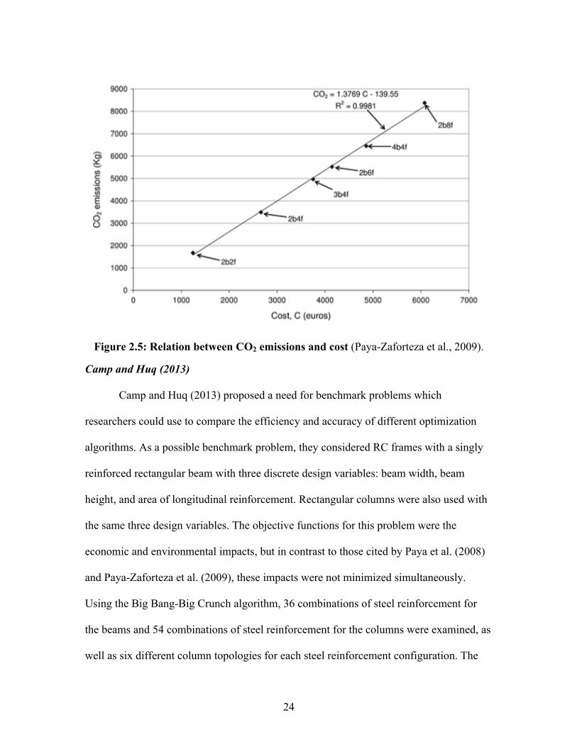
worsen CO2 emissions by 3.8%.” Figure 2.5 shows the multiobjective optimization of
different sized frames, and bears a linear relationship between the two objective
functions. Each data point consists of the letters “b” and “f.” The letter “b” represents the
number of bays and the letter “f” represents the number of floors.
24
Figure 2.5: Relation between CO2 emissions and cost (Paya-Zaforteza et al., 2009).
Camp and Huq (2013)
Camp and Huq (2013) proposed a need for benchmark problems which
researchers could use to compare the efficiency and accuracy of different optimization
algorithms. As a possible benchmark problem, they considered RC frames with a singly
reinforced rectangular beam with three discrete design variables: beam width, beam
height, and area of longitudinal reinforcement. Rectangular columns were also used with
the same three design variables. The objective functions for this problem were the
economic and environmental impacts, but in contrast to those cited by Paya et al. (2008)
and Paya-Zaforteza et al. (2009), these impacts were not minimized simultaneously.
Using the Big Bang-Big Crunch algorithm, 36 combinations of steel reinforcement for
the beams and 54 combinations of steel reinforcement for the columns were examined, as
well as six different column topologies for each steel reinforcement configuration. The

25
first example analyzed by the authors demonstrated the increased accuracy of the BB-BC
algorithm over the GA, with the best solution given by the BB-BC being 5.2% lower in
economic cost than the best solution produced by the GA. Two subsequent example
problems were conducted to evaluate the relationship of cost to CO2 emissions. In the
first example, the results demonstrated that “for a modest 2.2% increase in cost over the
low-cost design, a 10.2% reduction in CO2 emissions is achieved from the low cost
design.“ A similar result was given in the second example.
Yeo and Potra (2013)
Using the MATLAB optimization solver “fmincon,” which is a heuristic
optimization algorithm not capable of handling discrete variables, Yeo and Potra (2013)
examined a reinforced concrete single frame for lowest cost and CO2 emissions, each
individually. Beam design variables were the height, total area of the longitudinal
reinforcement, and spacing of the shear reinforcement; column design variables were
height, total area of the axial reinforcement, and spacing of the shear reinforcement. By
optimizing for CO2 emissions, a reduction of 5 to 15% of emissions was computed when
compared to the optimization of cost. In Figure 2.6(a), (b), and (c), rcost and rco2 represent
the “ratio between the cost of the cost-optimized frame and the cost of the CO2-optimized
frame” and “the ratio between the CO2 footprint of the cost-optimized frame and the CO2
footprint of the CO2-optimized frame,” respectively. RC and RCO2 represent the cost and
CO2 emission ratios, respectively, of steel to concrete. As the relative cost of steel
increases, the relative cost of the cost-optimized frame increases, but the relative CO2
emissions of the cost-optimized frame remain constant beyond a cost ratio of 0.8, as

26
demonstrated in Figure 2.6(a). The relative CO2 emissions of the steel have little to no
impact on the relative cost and relative CO2 emissions of the cost-optimized frame,
shown in Figure 2.6(b). Supplementary axial compressive forces of 3000 kN and 6000
kN were applied to the columns to provide a hypothetical gravity load induced by
additional floors. In Figure 2.6(c), the dependence upon concrete compressive strength of
rcost and rco2 is depicted for 30 MPa and 40 MPa, which causes little change between the
two.

27
Figure 2.6: (a) Dependence upon the cost ratio of the percentage of total cost and CO2 emissions for the cost-optimized frame and the CO2-optimized frame, (b) Dependence upon the CO2 ratio of the percentage of total cost and CO2 emissions for the cost-optimized frame and the CO2-optimized frame, (c), Dependence upon concrete compressive strength of the percentage of total cost and CO2 emissions for the cost-optimized frame and the CO2-optimized frame (Yeo & Potra, 2013).
2.4 Distinctions of Current Study
While each of these publications has a number of things in common with the
research being conducted in this paper, this section discusses the approaches that will be
used in the current research that are distinct from previous works.
a) b)
c)

28
Although algorithms are very powerful tools capable of shortening the
computational time considerably, they cannot be relied upon to obtain the global
optimum every time, sometimes returning a local minimum instead. By developing a list
of every combination of design variables, all permutations can be checked and the global
optimum is thus guaranteed for each optimization routine. This is not a novel concept and
requires additional computational time that is not always prudent. However, it does
promise complete accuracy not prevalent in other works.
The previous works have given only one optimum point for different cost ratios,
compressive strengths, steel ratios, and other parameters, but none have considered trends
in the optimal solutions. Taking averages rather than points has the potential to depict
overarching trends in near-optimized designs. Knowledge of such trends may be of
greater service to practicing engineers during the design phase when it is often
impractical to conduct rigorous optimization work to locate optimum points because
design parameters are still in flux. By enhancing the capacity of the optimization tool, the
complexity of the earlier models can be further developed.
Substituting concrete and steel with higher-strength materials is not the only way
to amplify the effects of optimization; LW aggregate, which abates the self-weight of the
concrete, can generate a smaller flexural moment. LW concrete, while more expensive,
reduces the volume of the beam and the materials required to support a known load or
moment. Previous works have not evaluated the benefits of LW concrete in optimal RC
design.

29
Although the embodied-energy factors of materials in reinforced concrete do not
fluctuate as significantly as cost factors, more efficient methods of producing concrete
and steel are being developed, which in turn reduces the embodied energy required to
manufacture RC beams. A unit embodied-energy ratio can be applied to complement the
unit cost ratio in the analysis of optimized beams. Using a range of these values in
various parametric studies, designers can select which ratio to use based on the current
status of steel or concrete.
2.5 Literature Review Summary
Based on the literature review of previous works, a few general conclusions can
be made about the reinforced concrete optimization.
According to Samman and Erbatur (1995) and Yeo and Potra (2013), the
compressive strength of concrete has little to no effect on the optimization of RC beams.
This conclusion is consistent with the well-known observation that compressive strength
also has minor effects on flexural capacity of beams relative to other design parameters.
Yeo and Gabbai (2011), Paya et al. (2008), Paya-Zaforteza et al. (2009), Camp
and Huq (2013), and Yeo and Potra (2013) all optimized for both economic and
environmental factors, demonstrating the trade-offs between each aspect. Yeo and Gabbai
(2011), Paya-Zaforteza et al. (2009), Camp and Huq (2013), and Yeo and Potra (2013)
conducted environmental optimization to show the effects over cost optimization. Yeo
and Gabbai (2011) optimized embodied energy, which resulted in a 10% reduction in
embodied energy for a 5% added cost; Paya-Zaforteza et al. (2009) optimized CO2
emissions for a 2.77% added cost; Camp and Huq (2013) optimized CO2 emissions,
30
which resulted in a 10.2% reduction in CO2 emissions for a 2.2% added cost; Yeo and
Potra (2013) optimized CO2 emissions for a 5-15% reduction in CO2 emissions when
compared to the optimized cost design. Each of these works exhibits similar results: for a
small increase in cost (around 2-5%), a larger percentage of energy can be saved (about
10%).
This is a partial list of cost and environmental optimization of reinforced concrete;
as a literature review, it only highlights what is most relevant to the research presented in
this thesis. For an extended bibliography of additional references pertaining to the
optimization of reinforced concrete structures, see page 127; this list can be used as a
gateway for more detailed analysis of RC structural optimization.

31
CHAPTER THREE
OPTIMIZATION OF REINFORCED CONCRETE BEAMS METHODOLOGY
3.1 Overview
This research considered rectangular reinforced concrete beams with simple
supports optimized for cost and embodied energy. Feasible beam designs were
constrained by the provisions of the ACI 318-11 code (ACI Committee 318, 2011).
Section 3.2 establishes the nomenclature used throughout this thesis. Wherever possible,
nomenclature was kept consistent with ACI 318. Sections 3.3 through 3.7 of this thesis
provide general descriptions of all design variables, parameters, and constraints used with
their respective ranges, as well as discussion of any assumptions made regarding the
configuration of steel reinforcement within the beam. The two computer programs, Excel
(Microsoft, 2011) and MATLAB (Mathworks, 2012), used in this research are also
discussed and compared. Section 3.8 provides more detail about the ACI code used and
how it was employed within the Excel computer program.
3.2 Nomenclature
Reinforced Concrete Design Definitions per ACI 318-11 Section 2.1
a = depth of equivalent rectangular stress block, in.
As = area of nonprestressed longitudinal tension reinforcement, in.2
Av = area of shear reinforcement within a distance s, in.2
b = width of compression face of member, in.
β1 =factor relating depth of equivalent rectangular compressive stress block to neutral
axis depth
32
c = distance from extreme compression fiber to neutral axis, in.
d = distance from extreme compression fiber to centroid of longitudinal tension
reinforcement, in.
dt = distance from extreme compression fiber to centroid of extreme layer of longitudinal
tension steel, in.
εt = net tensile strain in extreme layer of longitudinal tension steel at nominal strength
f’c = specified compressive strength of concrete, psi
fy = specified yield strength of reinforcement, psi
Mn = nominal flexural strength at section, lb-in.
ϕMn = design moment strength at section, lb-in.
Mu = factored moment at section, lb-in.
s = center-to-center spacing of shear ties measured along longitudinal axis of member
Vc = nominal shear strength provided by concrete, lb
Vn = nominal shear strength, lb
ϕVn = design shear strength at section, lb
Vu = factored shear force at section, lb
λ = modification factor reflecting the reduced mechanical properties of LW concrete
ϕ = strength reduction factor
Other Reinforced Concrete Design Definitions
csmin = minimum clear spacing between longitudinal reinforcement, in.
γ$C = unit cost of concrete, $/ft3
γ$S = unit cost of steel, $/ft3

33
ρ = reinforcement ratio [As /bh]
C = total cost of member, $
db = diameter of longitudinal reinforcement, in.
dmax_agg = maximum aggregate size in the mix, in.
ds = diameter of stirrups, in.
γEC = unit embodied energy of concrete, MJ/kg (MJ/lb)
γES = unit embodied energy of steel, MJ/kg (MJ/lb)
btrib = tributary width
EE = total embodied energy of member, MJ
L = span length of beam, ft
LW = lightweight
n = number of longitudinal reinforcement
ns = number of stirrups
NW = normal weight
Vstr = total volume of stirrups, in.3
wD = unfactored dead load, plf
wL = unfactored live load, plf
wS = unfactored self-weight, plf
wu = factored distributed load, plf
γc = unit weight of concrete, pcf
γs = unit weight of steel, pcf
34
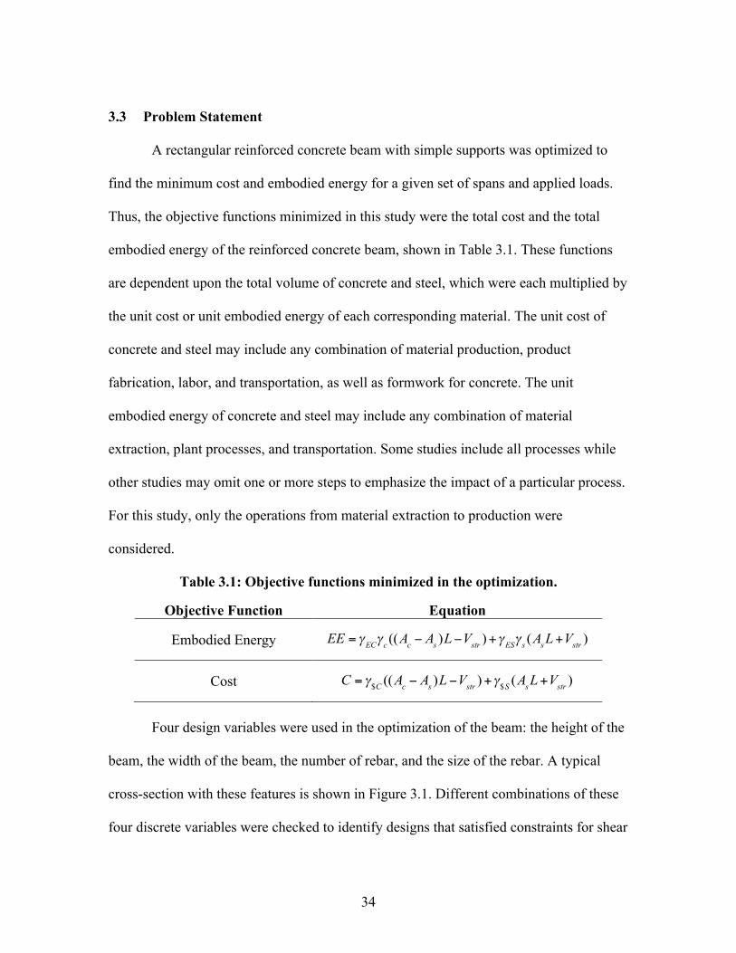
3.3 Problem Statement
A rectangular reinforced concrete beam with simple supports was optimized to
find the minimum cost and embodied energy for a given set of spans and applied loads.
Thus, the objective functions minimized in this study were the total cost and the total
embodied energy of the reinforced concrete beam, shown in Table 3.1. These functions
are dependent upon the total volume of concrete and steel, which were each multiplied by
the unit cost or unit embodied energy of each corresponding material. The unit cost of
concrete and steel may include any combination of material production, product
fabrication, labor, and transportation, as well as formwork for concrete. The unit
embodied energy of concrete and steel may include any combination of material
extraction, plant processes, and transportation. Some studies include all processes while
other studies may omit one or more steps to emphasize the impact of a particular process.
For this study, only the operations from material extraction to production were
considered.
Table 3.1: Objective functions minimized in the optimization.
Objective Function Equation
Embodied Energy EE = γECγc ((Ac − As )L−Vstr )+γESγ s (AsL+Vstr )
Cost C = γ$C ((Ac − As )L−Vstr )+γ$S (AsL+Vstr )
Four design variables were used in the optimization of the beam: the height of the
beam, the width of the beam, the number of rebar, and the size of the rebar. A typical
cross-section with these features is shown in Figure 3.1. Different combinations of these
four discrete variables were checked to identify designs that satisfied constraints for shear

35
and flexure as well as others. ACI 318 code requirements were used to establish
appropriate constraints. Up to 66,000 combinations of variables were considered in each
optimization problem, with each permutation consisting of a unique design. When
aggregated, this group of possible design permutations is referred to as the design space
of the optimization problem. A feasible set was then formed from all combinations that
satisfied the constraints (specified in Table 3.5). From the feasible set, the design with the
lowest total cost or embodied energy was chosen as the optimum solution.
Figure 3.1: Typical cross-section of a rectangular reinforced concrete beam.
3.4 Computer Programs
In this analysis, two separate optimization methods were utilized to obtain the
global minimum of either the total embodied energy or total cost of the reinforced
concrete beam. The first was a genetic algorithm, using the computer software
MATLAB. An objective function was written and constraints were defined; given four

36
discrete variables, a random number generator produced values for the four variables that
were fed through the constraint function and the objective function, converging on a
beam design that would minimize the objective function while still existing within the
limits set forth by the constraints. The design variables were returned for the optimum
design. All of this was accomplished through MATLAB’s built-in GA toolbox.
The second method used was the brute force method, which was executed using
the computer program Microsoft Excel. Instead of using a random number generator, all
66,000 combinations of the four discrete variables were individually analyzed. Through
an evaluation of every permutation, the global optimum was identified for each
optimization routine.
Both methods, MATLAB’s genetic algorithm and Excel’s brute force method, were
designed to check the accuracy of one another although each program has its advantages
and disadvantages. MATLAB is more flexible when adapting the design being tested,
whether it be expanding the design variables or altering the backbone of the design
altogether. One example of this would be transforming a rectangular cross-section into a
T-beam. Excel is much more rigid, requiring additional time and manipulation to adjust
the code for different conditions. However, with genetic algorithms, the global optimum
cannot always be assured; by going through every design combination in the brute force
method, the global optimum is guaranteed. Also, by using MATLAB, only a single point
can be obtained. With Excel, a top percentage of points can be determined and listed in
descending order. Analysis of multiple points can be helpful in evaluating trends that are
not evident by only considering a single optimum point.

37
Both programs were used in this study to verify one another, but after a preliminary
comparison of the MATLAB and Excel calculations, it was concluded that Excel was an
appropriate analysis tool for studying the relatively small design space presented in this
research. While using MATLAB’s GA would be a more efficient approach in larger
design spaces, it was not necessary for the current study. Therefore, all discussions of
optimization methodologies and results in this thesis are based on calculations using
Excel.
3.5 Design Variables
Design variables are those values that are altered within the design space when
locating the optimum solution. Four design variables were considered in this research
program: the height of the beam, the width of the beam, the number of rebar, and the size
of the rebar. Each variable was represented by a range of discrete values.
The range of values used for beam height, h, was selected based on the span
length, L, which is one of the design parameters discussed in the following section. This
range was selected based on the span length to ensure that values were realistic, that is,
not too large or too small for the span being considered.
For the beam height, a range from L/30 to L/10 was employed. The range
included twenty discrete values spaced evenly between the upper and lower limits; these
values were then rounded to the nearest half inch, as is typical for the cross-sectional
dimensions of RC beams.
The range of values for beam width, b, was a function of the range given for beam
height; thus, beam widths were also indirectly related to the span length of the beam,

38
ensuring that realistic values would be chosen for the span being considered. A range of
0.1h to h was employed in increments of 0.1, so that for each value of h there were ten
values of b. The width of the beam was also rounded to the nearest half inch but never
breached the boundaries defined by an upper and lower bound.
The third variable was the number of rebar, n, which ranged from two to twelve
bars. To produce a realistic representation of a reinforced concrete beam cross-section, up
to three layers of rebar were considered. A total of 33 configurations consisting of two to
twelve bars were used, shown in Figure 3.2. The final variable was the size of rebar,
which was based on standard bar sizes given by ASTM International A615, ranging from
#3 to #14 bars, listed in Table 3.2. Only a uniform selection of rebar was accepted for
each design. This means there could not be a medley of rebar sizes in a single design.
Each of the four variables was represented by discrete values, amounting to a design
space of 66,000 separate design combinations. Variables and combinations are
summarized in Table 3.3.

39
Figure 3.2: All configurations of longitudinal reinforcement utilized in the optimization of reinforcement concrete beams, categorized by number of rebar.
# Configurations
2 !!
!! ! !
3 !!
!! ! !
4 !!
!
!
!! !
5 !!
!
!
!! !
6 !!
!
!
!
!
! !
7 !!
!
!
! !!
8 !!
!
!
!
!
! !
9
!!!!!!
!
!!!
!
!!!
! !
10
!!!!
!
!!!!
!
!!!!
!
!
!
11
!!!
!
!!!
! !
!
12
!!
!!
!
!
! !
!!
! ! !
!
!!

40
The ACI 318-11 code provides minimum span-to-height ratios for which member
deflections need not be calculated. For some designers, these ratios become de facto
limits on member height. To account for this, some of the optimizations conducted in the
test program treated beam height as a fixed value (a parameter) based on the ACI ratios
rather than as a variable. For example, instead of appointing h a range from L/30 to L/10,
the height of the beam was given one constant value equal to the minimum beam height
required by the ACI 318-11 code in Table 9.5(a). For simply supported beams, L/16 is
given, but this only applies to NW concrete and 60 ksi steel reinforcement. For other
cases, L/16 was modified, as discussed in Section 3.8.5 of this chapter. In optimizations
where height was treated as a fixed parameter, the design space was condensed from
66,000 possible solutions to 3,300 possible solutions (Table 3.3).
The span-to-height ratios found in Table 9.5(a) of ACI 318-11 are the specified
minimum heights unless deflections are calculated. If, however, deflections are
calculated, it is permissible to design members that are more slender than the limits in
Table 9.5(a). While noting this distinction, member heights based on Table 9.5(a) will be
referred to as the “ACI minimum” throughout this thesis.

41
Table 3.2: ASTM standard chart for reinforcing steel bars considered in the optimization (ASTM International A615, 2012).
Bar Size Diameter (in.) Area (in.2) #3 0.375 0.11 #4 0.500 0.20 #5 0.625 0.31 #6 0.750 0.44 #7 0.875 0.60 #8 1.000 0.79 #9 1.128 1.00 #10 1.270 1.27 #11 1.410 1.56 #14 1.693 2.25
Table 3.3: Design variables considered in the optimization.
Variable Range Number of Variables
within Range
Height of Beam (h) L/30 to L/10
-or- (ACI minimum)
20 (1)
Width of Beam (b) 0.1h to h 10
Size of Reinforcement Bars
#3 to #14 See Table 3.2
10
Number of Reinforcement Bars (n)
2 to 12 bars In up to 3 layers
33
Total 66,000 (3,300)
3.6 Parameters
Parameters are values that are held constant in an optimization problem.
Parameters in the current program included span length of the beam, applied load, unit
cost and unit embodied energy of both concrete and steel, and unit weight of the concrete.

42
Although parameters are fixed for a given optimization calculation, they can be varied
from one individual calculation to another. For example, an optimization program could
be made to determine the optimal beam design for a given span length. The span length
could then be modified and the optimization program could repeat the calculation for the
new parameter. Evaluating changes in an optimum design for a single parameter will
emphasize the effects of that parameter on the entire system.
Span length and bending moment were among the parameters adjusted in
sequential optimization problems. Thus, trends in optimal designs were evaluated for a
range of spans and moments. Applied loads, and consequently applied moments, were
linked to the span length using the equations shown in Table 3.4. This approach was used
to improve the efficiency of sequential problems, and to ensure that the applied moments
were reasonable for each span length.
A range of moments from 50 k-ft to 9050 k-ft with increments of 150 k-ft was
used in all studies. The distributed loads were related to the span of the beam, also shown
in Table 3.4. As the span of the beam increases, the tributary width broadens at a
proportionate rate equal to one-fourth of the span length. So at a span of 20 ft, the
tributary width is 5 ft, and at a span of 60 ft, the tributary width is 15 ft.
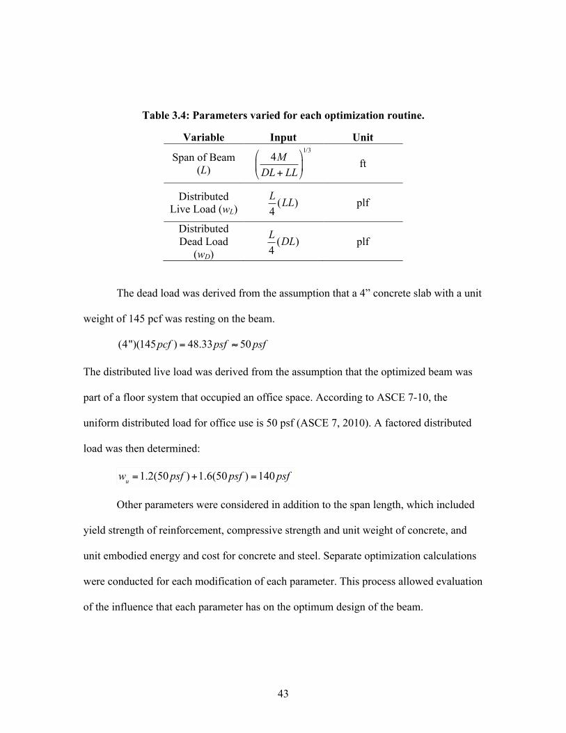
43
Table 3.4: Parameters varied for each optimization routine.
Variable Input Unit
Span of Beam (L) ft
Distributed Live Load (wL) plf
Distributed Dead Load
(wD) plf
The dead load was derived from the assumption that a 4” concrete slab with a unit
weight of 145 pcf was resting on the beam.
The distributed live load was derived from the assumption that the optimized beam was
part of a floor system that occupied an office space. According to ASCE 7-10, the
uniform distributed load for office use is 50 psf (ASCE 7, 2010). A factored distributed
load was then determined:
wu =1.2(50psf )+1.6(50psf ) =140psf
Other parameters were considered in addition to the span length, which included
yield strength of reinforcement, compressive strength and unit weight of concrete, and
unit embodied energy and cost for concrete and steel. Separate optimization calculations
were conducted for each modification of each parameter. This process allowed evaluation
of the influence that each parameter has on the optimum design of the beam.
4MDL+ LL!
"#
$
%&
1/3
L4(LL)
L4(DL)
(4")(145pcf ) = 48.33psf ≈ 50psf

44
3.7 Constraints
Constraints are properties of the system that must be satisfied in order for a given
solution to be deemed as feasible. For example, one constraint was flexural capacity.
Beam designs were only considered feasible if they satisfied the constraints of flexural
capacity and other constraints required by ACI 318-11. These other constraints included
nominal shear capacity, minimum beam width (to fit reinforcement), minimum and
maximum required area of steel, and required stirrup spacing. The maximum amount of
reinforcement, and by implication the ductility, was constrained by placing limits on
tensile strain in the lowest layer of reinforcement. Based on ACI 318-11, a minimum
strain of 0.004 was used for optimization problems that considered grade 60 steel
reinforcement. A separate net tensile strain constraint was applied to high-strength steel
reinforcement. This approach is consistent with the recommendations made by high-
strength reinforcement manufacturers (MMFX Technologies Corporation, 2012). All
constraints are summarized in Table 3.5.
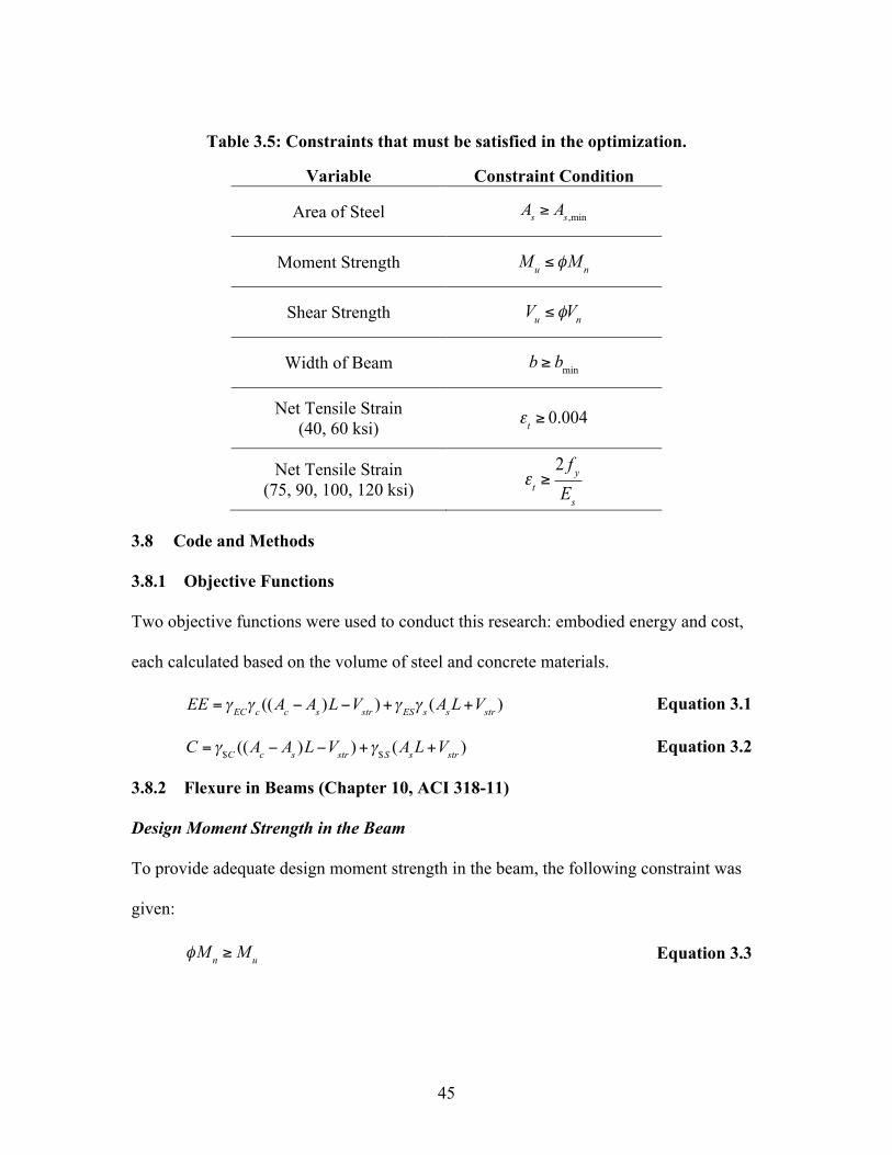
45
Table 3.5: Constraints that must be satisfied in the optimization.
Variable Constraint Condition
Area of Steel As ≥ As,min
Moment Strength Mu ≤ φMn
Shear Strength Vu ≤ φVn
Width of Beam b ≥ bmin
Net Tensile Strain (40, 60 ksi) εt ≥ 0.004
Net Tensile Strain (75, 90, 100, 120 ksi) εt ≥
2 f yEs
3.8 Code and Methods
3.8.1 Objective Functions
Two objective functions were used to conduct this research: embodied energy and cost,
each calculated based on the volume of steel and concrete materials.
EE = γECγc ((Ac − As )L−Vstr )+γESγ s (AsL+Vstr ) Equation 3.1
C = γ$C ((Ac − As )L−Vstr )+γ$S (AsL+Vstr ) Equation 3.2
3.8.2 Flexure in Beams (Chapter 10, ACI 318-11)
Design Moment Strength in the Beam
To provide adequate design moment strength in the beam, the following constraint was
given:
Equation 3.3
φMn ≥Mu

46
The nominal moment strength was calculated as
Mn = As f y d −a2
"
#$
%
&' Equation 3.4
The maximum factored moment in the beam was
Equation 3.5
where the factored distributed load is calculated by
wu =1.2(wD +wS )+1.6wL Equation 3.6
In order to calculate the design moment strength in the beam, several values must be
determined:
Equation 3.7
; f’c is in units of psi Equation 3.8
Equation 3.9
Equation 3.10
The strength reduction factor is calculated for two different ranges but is not to be taken
less than 0.004.
φ = 0.9 [εt ≥ 0.005] Equation 3.11
φ = 0.48+83εt [0.004 ≤ εt ≤ 0.005] Equation 3.12
Mu =wuL
2
8
a =As f y
0.85 f 'c b
β1 = 0.85≥ 0.85−0.05f 'c− 40001000
#
$%
&
'( ≥ 0.65
c = aβ1
εt =0.003(dt − c)
c

47
3.8.3 Shear in Beams (Chapter 11, ACI 318-11)
To provide shear reinforcement, #3 closed looped stirrups were equipped. Stirrup
placement was based on the required and maximum permitted spacing of stirrups for
shear in beams, which are detailed in Section 11.4 of ACI 318-11. Conditions for shear
design are given in Table 3.6 of this thesis.
Table 3.6: Stirrup design.
Stirrup Details Shear Condition
Figure 3.3 If
Figure 3.4 If
Figure 3.5 If
Required and maximum-permitted stirrup spacing, s
The maximum factored shear force was calculated using the equation
Equation 3.13
while the nominal shear strength of the concrete was calculated using the equation
Vc = 2λbd f 'c Equation 3.14
Stirrup spacing was then determined by one of three “if” statements:
1. If , then no stirrups were required and thus and . The shear
resistance factor is given as . The beam without stirrups is shown in
Figure 3.3.
Vu ≤φVc2
φVc2<Vu ≤ φVc
Vu > φVc
Vu =wuL2
Vu ≤φVc2
Av = 0 ns = 0
φs = 0.75

48
Figure 3.3: Beam without stirrups.
2. If , then , which is 0.11 in2 for a #3 bar. The spacing was
determined by finding the minimum of four values:
Equation 3.15
It is assumed that the stirrups extend into 1/6 of the span of the beam from each
support while the cover is accounted for at each end. Therefore, the number of
stirrups was calculated with the following equation:
Equation 3.16
Figure 3.4 shows the design of the beam with the spacing for the required number
of stirrups.
L
#3 @ s1 o.c. #3 @ s1 o.c.
L6
L6
#3 @ s2 o.c. #3 @ s1 o.c. #3 @ s1 o.c. #3 @ s2 o.c.
L6
L6
L6
L6!
φVc2<Vu ≤ φVc Av = Ab
s1 =minAv f y50b
,Av f y
0.75b f 'c, d2,24"
!
"
##
$
%
&&
ns = 2
L6− cover
s1+1
"
#
$$$$
%
&
''''
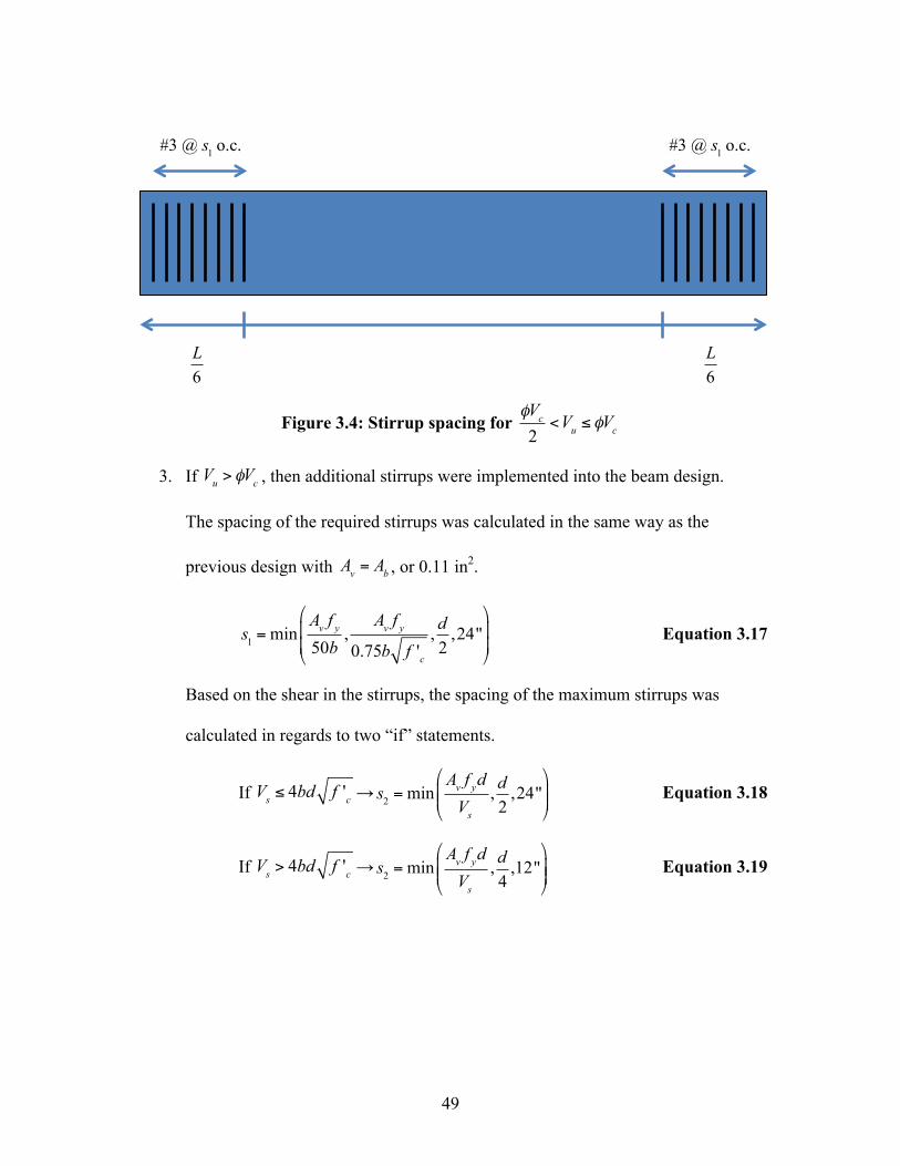
49
Figure 3.4: Stirrup spacing for
3. If , then additional stirrups were implemented into the beam design.
The spacing of the required stirrups was calculated in the same way as the
previous design with , or 0.11 in2.
Equation 3.17
Based on the shear in the stirrups, the spacing of the maximum stirrups was
calculated in regards to two “if” statements.
If → Equation 3.18
If → Equation 3.19
φVc2<Vu ≤ φVc
Vu > φVc
Av = Ab
s1 =minAv f y50b
,Av f y
0.75b f 'c, d2,24"
!
"
##
$
%
&&
Vs ≤ 4bd f 'c s2 =minAv f ydVs
, d2,24"
!
"##
$
%&&
Vs > 4bd f 'c s2 =minAv f ydVs
, d4,12"
!
"##
$
%&&
L
#3 @ s1 o.c. #3 @ s1 o.c.
L6
L6
#3 @ s2 o.c. #3 @ s1 o.c. #3 @ s1 o.c. #3 @ s2 o.c.
L6
L6
L6
L6!
!

50
The required reinforcement contribution to shear was estimated with the
following equation:
Equation 3.20
Figure 3.5 shows the design of the beam with both the spacing for the required
number of stirrups and the spacing for the maximum number of stirrups, each
expressed with s1 and s2, respectively.
Figure 3.5: Stirrup spacing for
Total Volume of Stirrups
The length of one stirrup was derived from the height and width of the beam, with the
cover being subtracted from each dimension. That value was then multiplied by the area
of a #3 bar and the total number of stirrups within the beam. This is an approximation
based on geometry.
Equation 3.21
Vs =minVu −φVc
φ,8bd f 'c
"
#$
%
&'
Vu > φVc
Vstr = (2(b− 2cover)+ 2(h− 2cover))Avns
L
#3 @ s1 o.c. #3 @ s1 o.c.
L6
L6
#3 @ s2 o.c. #3 @ s1 o.c. #3 @ s1 o.c. #3 @ s2 o.c.
L6
L6
L6
L6!
!

51
Single leg stirrups were assumed when calculating the spacing requirements for all
stirrups while the total volume of each stirrup was based on double leg stirrups. This had
the effect of increasing the volume of shear reinforcement calculated in the optimization
calculations. This approach was conservative but had very little impact on results. Shear
reinforcement typically contributed around 2-7% of the total embodied energy of the
beam (Figure 4.14). Also, the approach was applied consistently to all calculations so as
to not impede comparisons.
Design Shear Strength in the Beam
To ensure adequate design shear strength in the beam,
Equation 3.22
The nominal shear strength is given by
Equation 3.23
The nominal shear strength was not explicitly calculated by Vc + VS as provided by the
ACI code. Rather, Equation 3.23 was used as a simplified shear capacity calculation.
This simplification ensured that feasible solutions had sufficient shear strength but was
effectively of little consequence because shear rarely governed the optimum solutions.
3.8.4 Other Constraints
To ensure that the width of the beam was sufficient to accommodate the longitudinal and
shear reinforcement, a minimum width was computed for each combination of variables
using Equation 3.24.
Equation 3.24
φVn ≥Vu
Vn = 4 f 'cbd
bmin = 2(cover)+ 2ds + 2(2ds )+ (n−1)(db + csmin )

52
The minimum clear spacing, csmin, between adjacent longitudinal reinforcement was
based on the maximum of three values given by Section 7.6 in ACI 318-11:
Equation 3.25
The area of steel was subjected to two constraints: minimum and maximum area of steel.
A minimum area of steel is required to avoid brittle failure and the formation of cracks in
the concrete as the steel begins to yield; the subsequent equation indicates the minimal
area of steel permitted by Section 10.5 of ACI 318-11.
Equation 3.26
The maximum area of steel requirement was constrained by the net tensile strain
calculation (Equation 3.27) for yield strengths greater than 60,000 psi, which ensures that
the steel will yield in tension before the concrete crushes in compression.
Equation 3.27
Otherwise, the maximum area of steel requirement was constrained by a net tensile strain
value of 0.004.
3.8.5 Minimum Thickness for Nonprestressed Simply Supported Beams
While ACI 318-11 provides minimum span-to-height ratios for which member
deflections need not be calculated, a range of L/30 to L/10 was examined to study the
behavior of beams with a thickness below the ACI limits. The following equations are the
ACI minimum thicknesses for avoiding deflection calculations for nonprestressed simply
supported beams with various material properties:
csmin =max db ,1", 43 dmax_agg( )
As,min =max3 f 'cbdf y
, 200bdf y
!
"
##
$
%
&&
εt ≥2 f yEs
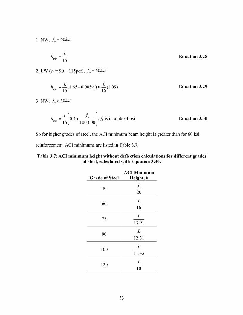
53
1. NW,
Equation 3.28
2. LW (γc = 90 – 115pcf),
hmin =L16(1.65−0.005γc ) ≥
L16(1.09) Equation 3.29
3. NW,
; fy is in units of psi Equation 3.30
So for higher grades of steel, the ACI minimum beam height is greater than for 60 ksi
reinforcement. ACI minimums are listed in Table 3.7.
Table 3.7: ACI minimum height without deflection calculations for different grades of steel, calculated with
Equation 3.30.
Grade of Steel ACI Minimum
Height, h
40
60
75
90
100
120
f y = 60ksi
hmin =L16
f y = 60ksi
f y ≠ 60ksi
hmin =L160.4+
f y100,000
!
"##
$
%&&
L20
L16
L13.91
L12.31
L11.43
L10

54
ACI minimums also changed for LW concrete relative to NW concrete. These values are
listed in Table 3.8.
Table 3.8: ACI minimum height without deflection calculations for different unit weights of concrete, calculated with
Equation 3.29.
Unit Weight of
Concrete ACI Minimum
Height, h
90
102.5
115
145
3.8.6 Comparisons with ACI 318-11
In addition to the discussion of ACI in previous sections, this section offers
clarifications regarding the application of ACI provisions to the research program.
Section 10.6.7 of ACI 318-11 requires that “longitudinal skin reinforcement shall
be uniformly distributed along both side faces of the member” when the height of the
beam, h, is greater than 36 inches. This provision was not considered in the research
program because it had minimal impact on the optimization results, which is explained in
detail below.
L13.33
L14.07
L14.68
L16
55
Skin reinforcement need only be distributed along half of the member’s depth.
Spacing is calculated using the following equation:
s =15 40,000fs
!
"##
$
%&&− 2.5cc Equation 3.31
The calculated stress in the reinforcement, fs, is permitted to be taken as 2/3fy, or 40,000.
The clear cover is assumed to be 1.5 inches for all optimization problems. With these
values defined, the smallest spacing required by ACI 318-11 is 11 inches. Because the
largest depth considered in the research program is 87 inches, 8 #3 bars is the maximum
number of skin reinforcement bars that is required. In an 87-inch deep member, 8 #3 bars
have very little influence on the total cost or total embodied energy of the beam.
The maximum concrete compressive strength considered in the test program was
10,000 psi. Strengths greater than this value trigger additional ACI requirements. For
example, Section 11.1.2 states that the values of that are used in Chapter 11 “shall
not exceed 100 psi” unless minimum shear reinforcement is provided in compliance with
provision 11.1.2.1. The additional provisions for higher strengths are mentioned here to
assist others in applying the methodology presented in this research.
ACI 318-11 also classifies 2,500 psi as the minimum allowable f’c for structural
concrete, stipulated in provision 1.1.1. Thus, 2,500 psi was the minimum value adopted
for concrete in this research.
In provision 10.7.2, deep beams (defined as beams with “clear spans equal to or
less than four times the overall member depth, h”) must meet the requirements set forth
f 'c

56
by Section 11.7. By constraining h to a maximum value of L/10, the optimized design of
the beam could never be categorized as a deep beam, so Section 11.7 did not apply.
Table 3.9 provides a summary of any ACI requirements that were modified in the
current research program.
Table 3.9: Summary of modifications to ACI 318-11
ACI Section ACI Requirement Modifications in
Research Program
10.6.7 Skin Reinforcement Did not consider skin reinforcement
11.1.2.1 Max f’c for Shear Unless
Minimum Shear Reinforcement Provided
Limited f’c to 10,000 psi
11.1.1 Nominal Shear Strengh
Table 9.5(a) Minimum Thickness without Deflection
Calculations
Limited ACI minimum thickness in some parametric studies
Vn = 4 f 'cbd

57
CHAPTER FOUR
PARAMETRIC STUDIES WITH EMBODIED ENERGY OPTIMIZED
4.1 Overview
In this chapter, several parametric studies have been conducted to analyze how
the flexural moment affects the design of beams optimized for embodied energy. Because
there have been fewer studies on the environmental impacts of reinforced concrete
design, the primary focus of this thesis centers on the effects of designing for reduced
embodied energy. However, cost is also considered in order to present a thorough
framework, and to compare results to previous studies for validation; cost-optimized
results can be found in Chapter 5.
Parametric studies were conducted to address two questions. First, what are the
relationships between different design variables of an RC beam optimized for embodied
energy? And second, how can different materials be quantitatively compared to assess
environmental preferability?
Explanation of Applied Moment
In all parametric studies, the moment is expressed as wL2. This quantity is
proportional to the maximum moment applied to the beam, with the distributed load, w,
consisting of the unfactored dead and live load. Because this considers the external
moment exclusively, the dead load does not include the self-weight of the beam. The self-
weight was included in the optimization calculations but not in the value of the
distributed load used in the figures. This approach was taken because self-weight is a

58
function of the design variables, which are not known at the beginning of the design
process.
Although all parametric studies in the next section deal with simply supported
beams and therefore have a maximum moment equal to wL2/8, results are reported in
terms of wL2 to normalize the data for comparison with future studies of beams with
alternative boundary conditions. While wL2 is not the flexural moment supported by the
beam, it will be referred to as such throughout this thesis. It should be noted that Mu was
calculated as wuL2/8 in all calculations.
Baseline Assumptions
A consistent set of baseline values was established for all optimization studies, as
listed in Table 4.1. Unless otherwise specified, each study was calculated with these
baseline values. Deviations from the baseline values are noted within the figures and/or
figure titles. Baseline values consist of the concrete and steel properties and the range of
span-to-depth ratios.

59
Table 4.1: Baseline assumptions and their alternate values for properties of concrete and steel. Baseline assumptions for the height of the beam are also included.
Variable Baseline Values Alternate Values Unit Compressive Strength of
Concrete (f’c) 4350 2500, 6000, 8000,
10000 psi
Yield Strength of Reinforcement (fy)
60 40, 75, 90, 100, 120 ksi
Unit Embodied Energy of Concrete (γEC) 1.3 0.65 - 3.25 MJ/kg
Unite Embodied Energy of Steel (γES)
8.9 4.45 - 22.25 MJ/kg
Unit Cost of Concrete (CC) 245 – $/ft3
Unit Cost of Steel (CS) 3.50 – $/ft3
Unit Weight of Concrete (γC) 145 90, 102.5, 115 pcf
Lightweight Modification Factor (λ) 1 0.75 unitless
Height of Beam (h) L/30 – L/10 ACI minimum in.
Figure 4.1 is an example of how the baseline values were applied. In this figure,
the optimum aspect ratios for six grades of steel were compared for varying flexural
moments; these grades are listed in the legend to the right of the figure. While the yield
strength of the steel varies from 60 ksi, one of the baseline values, the other parameters
remain fixed at the baseline values. The compressive strength of the concrete remains
4,350 psi; the unit embodied energy of concrete and steel remains 1.3 and 8.9 MJ/kg,
respectively; the unit weight of concrete remains 145 pcf; and the height of the beam is
calculated using the range of L/30 to L/10. Because this plot was optimized for embodied

60
energy, the cost of the materials did not contribute to the calculations and therefore does
not pertain to this particular study.
Figure 4.1: Example figure describing baseline and alternative values for parameters.
The same approach was applied in all calculations: If one or more of the baseline
assumptions is being modified within a figure, all other variables maintain their initial
baseline values. The alternate values are listed in Table 4.1 along with the baseline
values. Constant values that were assumed throughout all studies are featured in Table
4.2.
0.0 0.1 0.2 0.3 0.4 0.5 0.6 0.7 0.8 0.9 1.0
0
1000
2000
3000
4000
5000
6000
7000
8000
9000
Asp
ect R
atio
[b / h]
wL2 (k-ft)
40 ksi 60 ksi 75 ksi 90 ksi 100 ksi 120 ksi
Strength of Steel
L30
< h < L10
0.0 0.1 0.2 0.3 0.4 0.5 0.6 0.7 0.8 0.9 1.0
0
1000
2000
3000
4000
5000
6000
7000
8000
9000
Asp
ect R
atio
[b / h]
wL2 (k-ft)
40 ksi 60 ksi 75 ksi 90 ksi 100 ksi 120 ksi
Strength of Steel
h = ACI minimum

61
Table 4.2: Constant values assumed for all optimization calculations.
Variable Value Unit
Live Load (LL) 50 Psf
Dead Load (DL) 50 Psf
Diameter of Stirrup (ds) 0.375 in.
Area of Shear Reinforcement (Av)
0.11 in.2
Cover 1.5 in.
Diameter of Maximum Aggregate (dmax_agg)
0.8 in.
Unit Weight of Steel (γS) 490 Pcf
Unit Embodied Energy Values
A few sources identified the unit embodied energy for corresponding compressive
strengths and yield strengths of concrete and steel reinforcement, respectively. The values
are given in Table 4.3 with the steel-to-concrete ratios in the rightmost column. For the
parametric studies in this section, 1.3 MJ/kg was used as the unit embodied energy for
concrete, and 8.9 MJ/kg was used for steel reinforcement. Each of these values was taken
from “Table of embodied energy coefficients” (2007), and both correspond with the
baseline values used for concrete strength and steel grade. Unit embodied-energy
coefficients vary for materials with different properties, but based on limited data,
constant values were used throughout this study.

62
Table 4.3: Unit embodied energy for concrete and steel.1
Reference γEC γES
γESγEC
Alcorn (2003) 1.2 MJ/kg (0.5443 MJ/lb) (f’c = 4350 psi) 8.6 MJ/kg (3.901 MJ/lb) 7.17
Table of EE coefficients (2007)
1.3 MJ/kg (0.5897 MJ/lb) (f’c = 4350 psi) 8.9 MJ/kg (4.037 MJ/lb) 6.85
Hammond & Jones (2008)
1.39 MJ/kg (0.6305 MJ/lb) (high-strength) 8.80 MJ/kg (3.992 MJ/lb) 6.33
Yeo & Gabbai (2011)
1.37 MJ/kg (0.6210 MJ/lb) (f’c = 4930 psi)
8.9 MJ/kg (4.037 MJ/lb) (fy = 60,915 psi) 6.50
1Units given in SI were converted to U.S. customary Methodology for Presenting Parametric Study Results
Results of parametric studies are presented with four primary types of figures.
The first is a contour plot; all data in these plots have been normalized according to the
baseline assumptions so that direct comparisons can be made between different materials.
In Figure 4.2, for example, 75 ksi steel reinforcement was compared to 60 ksi steel
reinforcement (the baseline value) by dividing the unit embodied-energy ratio of 75 ksi
steel by the unit embodied-energy ratio of 60 ksi steel. The other three plots are scatter
plots which show the optimum cross-section properties as a function of the applied
moment. This section discusses how these plots were created and how they can be used to
interpret research results. Section 4.3 gives an example demonstrating the application of
these types of plots.
The contour plots are useful for comparing the preferability of different types of
material. An example of this type of plot is shown in Figure 4.2, which compares the
environmental preferability of grade 75 and grade 60 reinforcement. The y-axis of Figure

63
4.2 is the ratio of unit embodied energy between the materials being compared. For this
example, the unit embodied energy of grade 75 reinforcement is divided by the unit
embodied energy of 60 ksi steel (the baseline value). Ratios from 0.5 to 2.5 are reflected
upon the y-axis of the plot. On the x-axis, the flexural moment supported by the beam is
plotted, ranging from 50 to 9050 k-ft. A third value is represented by the different color
regions on the plot; this value is the total embodied energy of an optimum beam with 75
ksi steel, divided by the total embodied energy of an optimum beam with 60 ksi steel.
Data in the contour and scatter plots were generated through sequential
optimization problems that considered changes in the span-length parameter. Source data
from each optimization problem is not a single optimum point but instead is the average
of the top ten optimum points. For example, the aspect ratio was calculated for the top ten
optimum designs for a specific span length and unit embodied-energy coefficient. These
ten aspect ratios were then averaged and plotted as a single point on the scatter plot. The
same approach was taken for all studies because the designer may not be interested in an
individual point that limits the design of a beam.

64
Figure 4.2: Example figure comparing the embodied energy ratios for 60 ksi and 75 ksi steel reinforcement.
The different color regions in Figure 4.2 represent a percent increase or decrease
in total embodied energy, as defined in the legend. In the red region, the optimum beam
with 60 ksi steel has a lower total embodied energy than the optimum beam with 75 ksi
steel; the inverse of this is true in the blue region. The approximate border between these
two regions is portrayed by a dashed line; when above the dashed line, 60 ksi is
preferable to minimize embodied energy, but while below the dashed line, 75 ksi is
preferable.
The purpose of this class of plots is to show a large range of unit embodied-
energy ratios (Chapter 4) or unit cost ratios (Chapter 5) because the unit embodied-
energy and unit cost factors of different types of steel and concrete are uncertain and vary
geographically as well as over time. Instead of limiting this data to a specific region or
time in history, plots were generated to help designers apply research results to their
specific conditions.
0.50
0.75
1.00
1.25
1.50
1.75
2.00
2.25
2.50
50
800
1550
23
00
3050
38
00
4550
53
00
6050
68
00
7550
83
00
9050
γ E75
/ γ E
60
wL2 (k-ft)
1.30-1.40 1.20-1.30 1.10-1.20 1.00-1.10 0.90-1.00 0.80-0.90 0.70-0.80 0.60-0.70
Use 60 ksi
Use 75 ksi 50
5250
60
00
6750
75
00
3000
37
50
2250
1500
750
4500
9000
8250
L30
< h < L10
0.50
0.75
1.00
1.25
1.50
1.75
2.00
2.25
2.50
50
800
1550
23
00
3050
38
00
4550
53
00
6050
68
00
7550
83
00
9050
γ E75
/ γ E
60
wL2 (k-ft)
1.30-1.40 1.20-1.30 1.10-1.20 1.00-1.10 0.90-1.00 0.80-0.90 0.70-0.80 0.60-0.70
Use 60 ksi
Use 75 ksi
50
5250
60
00
6750
75
00
3000
37
50
2250
1500
750
4500
9000
8250
EE75
EE60
h = ACI minimum
0.9 - 1.0
> 1.3 1.2 - 1.3 1.1 - 1.2 1.0 - 1.1
0.8 - 0.9 0.7 - 0.8 < 0.7

65
The other three plots used to describe the parametric study results are all scatter
plots, which describe the aspect (b/h), reinforcement (As/(bh)), and span-to-depth (L/h)
ratios needed to design optimum cross sections. The flexural moment supported by the
beam is plotted along the x-axis, and one of the three ratios is plotted along the y-axis.
Like the contour plots, the top ten ratio values from each optimization routine were
averaged together for each point along the curve. A separate optimization routine was run
for each value of moment.
These four types of plots are divided into multiple subcategories. All plots
consider either the strength of concrete, the strength of steel, or the unit weight of
concrete with either the embodied energy (Chapter 4) or the cost (Chapter 5) optimized.
Separate parametric studies were also conducted to evaluate the effects of using the
minimum thickness values from ACI table 9.5(a). ACI requires deflection calculations
for members not meeting the minimum thickness values. Because the baseline range for
thickness (L/30 to L/10) included thickness values less than the ACI minimum, the
separate studies were conducted by changing the thickness of the beam to a constant
value equal to the minimum value prescribed by ACI; this reduced the design space from
66,000 possible solutions to 3,300 possible solutions.
In addition to the studies above, another study was performed to investigate how
the optimal values of each ratio (aspect, reinforcement, and span-to-depth) would be
affected by modifying unit embodied energy from the baseline value; these studies are
presented in both Section 4.3.1.3 (steel reinforcement) and Appendix A (concrete).
Modifications included a decrease of the baseline by 50% and an increase by 150%,

66
allowing evaluations over the same range considered in the contour plots. An example is
shown in Figure 4.5, where the baseline unit embodied energy of 8.9 MJ/kg of steel was
multiplied by 0.5 and 2.5, producing a unit embodied energy of 4.45 and 22.25 MJ/kg,
respectively. If a designer were to know the unit embodied energy of the material being
used, he could interpolate between the two plots. While values may not be linearly
related, this estimate is a product of two plots that show little variance between each
other; therefore, it is reasonable to use linear interpolation since a refined analysis would
be unlikely to produce significantly different results.
Example Application of Parametric Study Results
To demonstrate the application of each type of plot, a design example is
presented. Table 4.4 and Figure 4.3 give the values chosen for this example. In the
example, the preferability of 60ksi and 75ksi reinforcement will be evaluated. After the
environmentally preferred reinforcement is identified, a cross-section with near-minimum
embodied energy will be designed.

67
Table 4.4: Design example values
Variable Value wL, wD 50 psf
L 50 ft
btrib 12.5 ft
f’c 4,350 psi
fy 60 ksi, 75 ksi
γEC 1.3 MJ/kg
γES 10 MJ/kg
γc 145 pcf
Figure 4.3: Design example of simply supported beam exposed to distributed load.
To interpret the contour plots, the applied moment and unit embodied-energy ratio must
be computed. For the example, the moment is calculated as
M*= (wD +wL )(btrib )L2 = (100psf )(12.5 ft)(50 ft2 ) 1k
1,000 ft!
"#
$
%&= 3,125k ⋅ ft
wL!=!50!psf,!wD!=!50!psf!
L!=!50!)!

68
The unit embodied-energy ratio for the materials being compared is also needed. For the
given values of 10 MJ/kg for 75 ksi steel, and 8.9MJ/kg for 60 ksi steel, the ratio is
γE75γE60
=10MJ / kg8.9MJ / kg
=1.124
By presenting the optimization results in this manner, the results can be used to evaluate
preferability of materials having a wide range of unit embodied-energy values.
Figure 4.4 is a contour plot that demonstrates the decision-making aspect of this
example. This plot was used to establish which type of reinforcement, 75 ksi or 60 ksi, is
preferable from an environmental standpoint. The applied moment and unit embodied-
energy ratio are represented on the plot by two solid black lines. Because these two lines
intersect in the blue region, 75 ksi is the desirable strength of steel reinforcement.
Figure 4.4: Design example comparing the embodied-energy ratios for 60 ksi and 75 ksi steel reinforcement.
Since grade 75 steel was established as the preferable strength of reinforcement,
Figure 4.5 through Figure 4.7 were utilized to determine the near-optimum cross-
sectional characteristics of reinforced concrete with 75 ksi steel reinforcement. Figure 4.5
0.50
0.75
1.00
1.25
1.50
1.75
2.00
2.25
2.50
50
800
1550
23
00
3050
38
00
4550
53
00
6050
68
00
7550
83
00
9050
γ E75
/ γ E
60
wL2 (k-ft)
1.30-1.40 1.20-1.30 1.10-1.20 1.00-1.10 0.90-1.00 0.80-0.90 0.70-0.80 0.60-0.70
Use 60 ksi
Use 75 ksi
50
5250
60
00
6750
75
00
3000
37
50
2250
1500
750
4500
9000
8250
EE75
EE60
h = ACI minimum
0.9 - 1.0
> 1.3 1.2 - 1.3 1.1 - 1.2 1.0 - 1.1
0.8 - 0.9 0.7 - 0.8 < 0.7
0.50
0.75
1.00
1.25
1.50
1.75
2.00
2.25
2.50
50
800
1550
23
00
3050
38
00
4550
53
00
6050
68
00
7550
83
00
9050
γ E75
/ γ E
60
wL2 (k-ft)
1.30-1.40 1.20-1.30 1.10-1.20 1.00-1.10 0.90-1.00 0.80-0.90 0.70-0.80 0.60-0.70
Use 60 ksi
Use 75 ksi
50
5250
60
00
6750
75
00
3000
37
50
2250
1500
750
4500
9000
8250
L30
< h < L10
γE75 / γE60 = 1.124
M* = 3,125 k-ft

69
depicts two plots: The one on the left is one-half the baseline unit embodied energy, or
4.45 MJ/kg; the one on the right is two-and-a-half times the baseline unit embodied
energy, or 22.25 MJ/kg. With a moment of 3125 k-ft, the aspect ratio was determined for
each plot (0.243 for Figure 4.5(a) and 0.217 for Figure 4.5(b)). To estimate the optimum
aspect ratio proportional to 10 MJ/kg, interpolation was executed utilizing the two values
previously identified. This resulted in an aspect ratio of 0.235. It is unknown if the
transition occurring between each plot is linear, but because the two values are so close,
this interpolated value is a close approximation of the optimum value.
Figure 4.5: Design example demonstrating the effects of the unit embodied-energy ratio of steel on the aspect ratio. (a) One-half the baseline unit embodied energy of
steel, (b) Two-and-a-half times the baseline unit embodied energy of steel.
The same approach was used in Figure 4.6 and Figure 4.7. From Figure 4.6, the
reinforcement ratio for 10 MJ/kg was 0.0119. From Figure 4.7, the span-to-depth ratio for
10 MJ/kg was 15.34.
0.0 0.1 0.2 0.3 0.4 0.5 0.6 0.7 0.8 0.9 1.0
0
1000
2000
3000
4000
5000
6000
7000
8000
9000
Asp
ect R
atio
[b / h]
wL2 (k-ft)
40 ksi 60 ksi 75 ksi 90 ksi 100 ksi 120 ksi
Strength of Steel
γES = 4.45 MJ/kg
0.0 0.1 0.2 0.3 0.4 0.5 0.6 0.7 0.8 0.9 1.0
0
1000
2000
3000
4000
5000
6000
7000
8000
9000
Asp
ect R
atio
[b / h]
wL2 (k-ft)
40 ksi 60 ksi 75 ksi 90 ksi 100 ksi 120 ksi
Strength of Steel
γES = 22.25 MJ/kg
0
5
10
15
20
25
30
35
40
45
50
0
1000
2000
3000
4000
5000
6000
7000
8000
9000
% F
easi
ble
Sol
utio
ns
wL2 (k-ft)
40 ksi 60 ksi 75 ksi 90 ksi 100 ksi 120 ksi
Strength of Steel
L30
< h < L10
a) b)

70
Figure 4.6: Design example demonstrating the effects of the unit embodied-energy ratio of steel on the reinforcement ratio. (a) One-half the baseline unit embodied
energy of steel, (b) Two-and-a-half times the baseline unit embodied energy of steel.
Figure 4.7: Design example demonstrating the effects of the unit embodied-energy ratio of steel on the span-to-depth ratio. (a) One-half the baseline unit embodied
energy of steel, (b) Two-and-a-half times the baseline unit embodied energy of steel.
Having established all of these ratios, the design variables were calculated as follows:
Lh=15.34→ h = 50 ft
15.3412in1 ft
"
#$
%
&' ≈ 39.5in
bh= 0.235→ b = 50 ft
15.34(0.235) 12in
1 ft"
#$
%
&' ≈ 9.5in
ρ =Asbh
= 0.0119→ As =50 ft15.34"
#$
%
&'
2
(0.235)(0.0119) 144in2
1 ft2"
#$
%
&' ≈ 4.21in2 or 7 #7 bars
0.000
0.005
0.010
0.015
0.020
0.025
0.030
0.035
0
1000
2000
3000
4000
5000
6000
7000
8000
9000
Rei
nfor
cem
ent R
atio
[ρ]
wL2 (k-ft)
40 ksi 60 ksi 75 ksi 90 ksi 100 ksi 120 ksi
Strength of Steel
γES = 4.45 MJ/kg
0.000
0.005
0.010
0.015
0.020
0.025
0.030
0.035
0
1000
2000
3000
4000
5000
6000
7000
8000
9000
Rei
nfor
cem
ent R
atio
[ρ]
wL2 (k-ft)
40 ksi 60 ksi 75 ksi 90 ksi 100 ksi 120 ksi
Strength of Steel
γES = 22.25 MJ/kg
0
5
10
15
20
25
30
35
40
45
50
0
1000
2000
3000
4000
5000
6000
7000
8000
9000
% F
easi
ble
Sol
utio
ns
wL2 (k-ft)
40 ksi 60 ksi 75 ksi 90 ksi 100 ksi 120 ksi
Strength of Steel
L30
< h < L10
8
10
12
14
16
18
20
22
24
26
0
1000
2000
3000
4000
5000
6000
7000
8000
9000
Spa
n-to
-Dep
th R
atio
[L /
h]
wL2 (k-ft)
40 ksi 60 ksi 75 ksi 90 ksi 100 ksi 120 ksi
Strength of Steel
γES = 4.45 MJ/kg
8
10
12
14
16
18
20
22
24
26
0
1000
2000
3000
4000
5000
6000
7000
8000
9000
Spa
n-to
-Dep
th R
atio
[L /
h]
wL2 (k-ft)
40 ksi 60 ksi 75 ksi 90 ksi 100 ksi 120 ksi
Strength of Steel
γES = 22.25 MJ/kg
0
5
10
15
20
25
30
35
40
45
50
0
1000
2000
3000
4000
5000
6000
7000
8000
9000
% F
easi
ble
Sol
utio
ns
wL2 (k-ft)
40 ksi 60 ksi 75 ksi 90 ksi 100 ksi 120 ksi
Strength of Steel
L30
< h < L10
a) b)
a) b)

71
The cross-section derived from the design process is shown in Figure 4.8. Because these
values were calculated using averages of the top ten optimum points and because some
rounding occurred, it is important for the designer to verify that these design variables
meet the constraint criteria described in Section 3.8.
Figure 4.8: Cross-section of design example, drawn to scale.
Validation
Where possible, the methodology presented in this study has been compared and
validated using results of the previous works discussed in Chapter 2. Optimization of the
reinforcement ratio for embodied energy and cost were both considered for validation and
are later examined in Section 4.3 and Section 5.2, respectively.
Using 25 MPa (≈ 3,625 psi) concrete and 400 MPa (≈ 58 ksi) steel, Alreshaid et
al. (2004) established that the recommended reinforcement ratio for beams is about
h
b
As%

72
0.0154 when optimized for cost, which is close to the 0.0149 ratio obtained in the current
study for beams with 4,350 psi concrete and 60 ksi steel optimized for embodied energy.
However, when optimized for cost, the recommended steel ratio was only 0.0124. This is
in large part due to fluctuating steel-to-concrete unit cost ratios and different problem set-
ups. Also, the reinforcement ratio was defined as As/(bh) in this study but was defined as
As/(bd) in Alreshaid et al. (2004). Therefore, the reinforcement ratio results will have
slightly smaller values in this study. The recommended ratios are shown in Figure 4.9.
Figure 4.9: Recommended reinforcement ratio comparisons to Alreshaid et al. (2004) for 60 ksi steel reinforcement.
In Section 2.5 of this thesis, the results for the simultaneous optimization of
embodied energy and cost are summarized for each study in the literature review. One
example is the work of Yeo and Potra (2013), which stated that optimizing for CO2
emissions culminated in a 5-15% reduction in CO2 emissions when compared to the
optimized cost design. The results from Yeo and Poltra are similar to the results obtained
in the current study as shown in Figure 4.10. This figure presents the ratio of total
embodied energy for cost and energy optimum solutions. The percentage difference in
energy was between 1% and 11%, which is similar in magnitude to the results from Yeo
0.0149 0.0124
0.0154
0.000
0.005
0.010
0.015
0.020
0.025
0.030
0.035
Optimum EE (Kosloski, 2013)
Optimum Cost (Kosloski, 2013)
Optimum Cost (Alreshaid et al.,
2004)
Rec
omm
ende
d R
einf
orce
men
t Rat
io [ρ
] L30
< h < L10

73
and Potra, as well as other researchers. Further analysis on multiobjective optimization is
given in Section 5.2.4.
Figure 4.10: Total embodied energy of the cost-optimized design divided by the total embodied energy of the embodied-energy optimized design with variable span-to-
depth ratio
4.2 Effects of Parameters on Problem Set-Up
Section 4.2 presents general information about the optimization results.
Information in this section is based on–and provides context for–the parametric studies
presented in subsequent sections.
4.2.1 Percentage of Feasible Solutions in each Study
Figure 4.11, Figure 4.12, and Figure 4.13 demonstrate the percentage of feasible
solutions within the design space as the span lengths and moments changed. Feasible
solution percentages from each parametric study in this research are represented by these
six plots: strength of steel, strength of concrete, and unit weight of concrete, each one
divided into the two ranges given to the height of the beam throughout this paper. The
percentage is based on 66,000 possible solutions for the baseline case of L/30 < h < L/10
and 3,300 possible solutions for h = ACI minimum. A higher strength in steel and
concrete and a lower unit weight of concrete tend to generate more solutions. As the yield
0.85
0.90
0.95
1.00
1.05
1.10
1.15
0 10
00
2000
30
00
4000
50
00
6000
70
00
8000
90
00
EEC
ost_
Opt
/ EE
EE_O
pt
wL2 (k-ft)
L30
< h < L10

74
strength of steel increases, the nominal moment capacity also increases, producing more
feasible solutions. Yet as the compressive strength of the concrete increases, the nominal
moment capacity increases slightly and the nominal shear capacity increases
significantly, producing a slight boost in the percentage of solutions that are feasible; the
slight increase is in response to the moment governing over the shear in most
circumstances. When the unit weight of concrete is reduced, the factored shear force and
the factored moment lessen, resulting in a higher percentage of feasible solutions.
At short spans with less moment, fewer solutions are feasible. This occurred
because many of the reinforcement bar sizes and configurations had too much steel to be
practical for beams carrying small moments. This condition was manifested in the
calculations when the calculated neutral axis depth, c, was greater than the effective
flexural depth, dt. Such conditions are physically meaningless in reinforced concrete
mechanics and were just a function of the values used for the variables. At long spans
with larger moment, the percentage of feasible solutions began to decline due to the
increase in the factored shear force and the factored moment.
Figure 4.11: Percentage of possible solutions that are feasible for different grades of steel reinforcement. (a) Variable span-to-depth ratio, (b) ACI minimum depth.
0
5
10
15
20
25
30
35
40
45
50
0
1000
2000
3000
4000
5000
6000
7000
8000
9000
% F
easi
ble
Sol
utio
ns
wL2 (k-ft)
40 ksi 60 ksi 75 ksi 90 ksi 100 ksi 120 ksi
Strength of Steel
L30
< h < L10
0
5
10
15
20
25
30
35
40
45
50
0
1000
2000
3000
4000
5000
6000
7000
8000
9000
% F
easi
ble
Sol
utio
ns
wL2 (k-ft)
40 ksi 60 ksi 75 ksi 90 ksi 100 ksi 120 ksi
Strength of Steel
h = ACI minimum
0
5
10
15
20
25
30
35
40
45
50
0
1000
2000
3000
4000
5000
6000
7000
8000
9000
% F
easi
ble
Sol
utio
ns
wL2 (k-ft)
40 ksi 60 ksi 75 ksi 90 ksi 100 ksi 120 ksi
Strength of Steel
L30
< h < L10
a) b)

75
Figure 4.12: Percentage of possible solutions that are feasible for different grades of concrete. (a) Variable span-to-depth ratio, (b) ACI minimum depth.
Figure 4.13: Percentage of possible solutions that are feasible for different unit weights of concrete. (a) Variable span-to-depth ratio, (b) ACI minimum depth.
4.2.2 Contribution of Shear Reinforcement
Several assumptions were made to simplify the calculations necessary for the
computation of the shear reinforcement, which have been expressed in detail as part of
Section 3.8.3. Although they are all well-informed assumptions based on engineering
judgment, it is desirable to know what impact the shear reinforcement has on the total
embodied energy and total cost. Figure 4.14(a) and Figure 4.15(a) show that the shear
reinforcement contributed to less than 4% of the total embodied energy and less than 7%
of the total cost for beams with moments greater than 800 k-ft. In Figure 4.14(b) and
Figure 4.15(b), the shear reinforcement contributed to less than 4% of the total embodied
0
5
10
15
20
25
30
35
40
45
50
0
1000
2000
3000
4000
5000
6000
7000
8000
9000
% F
easi
ble
Sol
utio
ns
wL2 (k-ft)
2,500 psi
4,350 psi
6,000 psi
8,000 psi
10,000 psi
Strength of Concrete
L30
< h < L10
0
5
10
15
20
25
30
35
40
45
50
0
1000
2000
3000
4000
5000
6000
7000
8000
9000
% F
easi
ble
Sol
utio
ns
wL2 (k-ft)
2,500 psi
4,350 psi
6,000 psi
8,000 psi
10,000 psi
Strength of Concrete
h = ACI minimum
0.000
0.005
0.010
0.015
0.020
0.025
0.030
0.035
0
1000
2000
3000
4000
5000
6000
7000
8000
9000
Rei
nfor
cem
ent R
atio
[ρ ]
wL2 (k-ft)
2,500 psi 4,350 psi 6,000 psi 8,000 psi 10,000 psi
Strength of Concrete
L30
< h < L10
0 5
10 15 20 25 30 35 40 45 50
0
1000
2000
3000
4000
5000
6000
7000
8000
9000
% F
easi
ble
Sol
utio
ns
wL2 (k-ft)
90 pcf 103 pcf 115 pcf 145 pcf
Unit Weight of Concrete
L30
< h < L10
0 5
10 15 20 25 30 35 40 45 50
0
1000
2000
3000
4000
5000
6000
7000
8000
9000
% F
easi
ble
Sol
utio
ns
wL2 (k-ft)
90 pcf 103 pcf 115 pcf 145 pcf
Unit Weight of Concrete
h = ACI minimum
0.0 0.1 0.2 0.3 0.4 0.5 0.6 0.7 0.8 0.9 1.0
0
1000
2000
3000
4000
5000
6000
7000
8000
9000
Asp
ect R
atio
[b / h]
wL2 (k-ft)
90 pcf 103 pcf 115 pcf 145 pcf
Unit Weight of Concrete
γEC = 0.65 MJ/kg
a) b)
a) b)

76
energy and less than 7% of the total cost for beams with moments greater than 500 k-ft.
Thus, in most examples, any assumptions made with regard to shear reinforcement have
small ramifications on the total output of the problem.
Figure 4.14: Contribution of 60 ksi shear reinforcement to the total embodied energy of the beam. (a) Variable span-to-depth ratio, (b) ACI minimum depth.
Figure 4.15: Contribution of 60 ksi shear reinforcement to the total cost of the beam. (a) Variable span-to-depth ratio, (b) ACI minimum depth.
4.2.3 Average Number of Layers in Optimum Designs
Many variables define the design space in this research. One among these is the
number of rebar, arranged in one, two, or three layers. All configurations considered for
the optimization problem at hand are shown in Figure 3.2.
0
2
4
6
8
10
12
14
16
0 10
00
2000
30
00
4000
50
00
6000
70
00
8000
90
00
% E
E fo
r S
hear
Rei
nfor
cem
ent
wL2 (k-ft)
L30
< h < L10
0
2
4
6
8
10
12
14
16
0 10
00
2000
30
00
4000
50
00
6000
70
00
8000
90
00
% E
E fo
r S
hear
Rei
nfor
cem
ent
wL2 (k-ft)
h = ACI minimum
0
2
4
6
8
10
12
14
16
0 10
00
2000
30
00
4000
50
00
6000
70
00
8000
90
00 % C
ost f
or S
hear
Rei
nfor
cem
ent
wL2 (k-ft)
L30
< h < L10
0
2
4
6
8
10
12
14
16
0 10
00
2000
30
00
4000
50
00
6000
70
00
8000
90
00 %
Cos
t for
She
ar R
einf
orce
men
t
wL2 (k-ft)
h = ACI minimum
a) b)
a) b)

77
Figure 4.16 through Figure 4.18 convey the average number of layers in the top
ten embodied energy optimized designs. In most cases, the average number of layers
increases as the moment increases. That result suggests that some of the optimum
solutions for longer span beams may have benefitted from four or more layers of
reinforcement.
Overall, higher grades of steel resulted in optimized designs with fewer layers.
This is because it takes fewer high-strength bars (relative to lower-strength bars) to carry
tensile forces in the section. Another interpretation could be justified with Equation 3.4,
where a greater yield strength could take advantage of the increased effective depth
(which is a feature of fewer layers of reinforcement), thereby strengthening the nominal
moment capacity.
Compressive strength and unit weight of the concrete have a lesser impact on the
number of layers. Stronger concrete does not always minimize the demand for
reinforcement; however, this enhanced property does lessen the need for concrete, which
oftentimes results in optimum beams with thinner widths. One of the constraints in the
optimization routines was minimum beam width, which is governed by the widest layer
of reinforcement. When the beam width becomes smaller, more layers are needed to meet
the required nominal moment capacity. Therefore, stronger concrete may veer towards an
overall trend with additional layers of reinforcement.

78
Figure 4.16: Average number of layers of reinforcement for different grades of steel reinforcement when optimized for embodied energy. (a) Variable span-to-depth
ratio, (b) ACI minimum depth.
Figure 4.17: Average number of layers of reinforcement for different grades of concrete when optimized for embodied energy. (a) Variable span-to-depth ratio, (b)
ACI minimum depth.
Figure 4.18: Average number of layers of reinforcement for different unit weights of concrete when optimized for embodied energy. (a) Variable span-to-depth ratio, (b)
ACI minimum depth.
1.0
1.2
1.4
1.6
1.8
2.0
2.2
2.4
2.6
2.8
3.0
0
1000
2000
3000
4000
5000
6000
7000
8000
9000
Laye
rs o
f Rei
nfor
cem
ent
wL2 (k-ft)
40 ksi 60 ksi 75 ksi 90 ksi 100 ksi 120 ksi
Strength of Steel
L30
< h < L10
1.0
1.2
1.4
1.6
1.8
2.0
2.2
2.4
2.6
2.8
3.0
0
1000
2000
3000
4000
5000
6000
7000
8000
9000
Laye
rs o
f Rei
nfor
cem
ent
wL2 (k-ft)
40 ksi 60 ksi 75 ksi 90 ksi 100 ksi 120 ksi
Strength of Steel
h = ACI minimum 0.0 0.1 0.2 0.3 0.4 0.5 0.6 0.7 0.8 0.9 1.0
0
1000
2000
3000
4000
5000
6000
7000
8000
9000
Asp
ect R
atio
[b / h]
wL2 (k-ft)
40 ksi 60 ksi 75 ksi 90 ksi 100 ksi 120 ksi
Strength of Steel
h = ACI minimum
1.0
1.2
1.4
1.6
1.8
2.0
2.2
2.4
2.6
2.8
3.0
0
1000
2000
3000
4000
5000
6000
7000
8000
9000
Laye
rs o
f Rei
nfor
cem
ent
wL2 (k-ft)
2,500 psi
4,350 psi
6,000 psi
8,000 psi
10,000 psi
Strength of Concrete
L30
< h < L10 1.0
1.2
1.4
1.6
1.8
2.0
2.2
2.4
2.6
2.8
3.0
0
1000
2000
3000
4000
5000
6000
7000
8000
9000
Laye
rs o
f Rei
nfor
cem
ent
wL2 (k-ft)
2,500 psi
4,350 psi
6,000 psi
8,000 psi
10,000 psi
Strength of Concrete
h = ACI minimum 0.000
0.005
0.010
0.015
0.020
0.025
0.030
0.035
0
1000
2000
3000
4000
5000
6000
7000
8000
9000
Rei
nfor
cem
ent R
atio
[ρ ]
wL2 (k-ft)
2,500 psi 4,350 psi 6,000 psi 8,000 psi 10,000 psi
Strength of Concrete
L30
< h < L10
1.0
1.2
1.4
1.6
1.8
2.0
2.2
2.4
2.6
2.8
3.0
0
1000
2000
3000
4000
5000
6000
7000
8000
9000
Laye
rs o
f Rei
nfor
cem
ent
wL2 (k-ft)
90 pcf 103 pcf 115 pcf 145 pcf
Unit Weight of Concrete
L30
< h < L10
1.0
1.2
1.4
1.6
1.8
2.0
2.2
2.4
2.6
2.8
3.0
0
1000
2000
3000
4000
5000
6000
7000
8000
9000
Laye
rs o
f Rei
nfor
cem
ent
wL2 (k-ft)
90 pcf 103 pcf 115 pcf 145 pcf
Unit Weight of Concrete
h = ACI minimum 0.0 0.1 0.2 0.3 0.4 0.5 0.6 0.7 0.8 0.9 1.0
0
1000
2000
3000
4000
5000
6000
7000
8000
9000
Asp
ect R
atio
[b / h]
wL2 (k-ft)
90 pcf 103 pcf 115 pcf 145 pcf
Unit Weight of Concrete
γEC = 0.65 MJ/kg
a) b)
a) b)
a) b)

79
4.3 Parametric Studies
This section is devoted to parametric studies performed for the optimization of
embodied energy. For additional parametric studies on the optimization of embodied
energy, see Appendix A.
4.3.1 Variation of Steel Yield Strength
4.3.1.1 Selection of Optimum Steel Yield Strength
In this section, contour plots were developed to determine when different grades
of reinforcement would be preferable to grade 60 reinforcement when different unit
embodied-energy ratios are used. In the left column, results are based on an h ranging
from L/30 to L/10; in the right column, h was set equal to the minimum beam height
prescribed by ACI 318-11. Thus, instead of 20 values for h, only one constant value is
given for each grade of steel. For clarification, the range of h is labeled in each figure.
The flexural moment was plotted on the x-axis, with a range of 50 to 9050 k-ft in
increments of 150 k-ft. The unit embodied-energy ratio was plotted along the y-axis, with
a range of 0.5 to 2.5 to show a wide spectrum of realistic values.
Figure 4.19(a) shows a positive linear relationship between the flexural moment
and the unit embodied-energy ratio. As the strength of the steel increases (Figure
4.20(a)), the trend becomes steeper and more erratic, having periods of highs and lows.
Both conditions demonstrate that as the moment increases, it is more efficient to use
higher-grade steel.
Figure 4.19(b) and Figure 4.20(b) do not share the same trends as their L/30 to
L/10 counterparts. While an increase in the moment does prove to be a selling point for

80
75 ksi steel reinforcement (Figure 4.19(b)), 120 ksi steel is not supported by favorable
results (Figure 4.20(b)), with 60 ksi steel being the superior choice in most
circumstances. (See Appendix A for other standard steel reinforcement grades.)
Figure 4.19: Comparison of embodied-energy ratios for 60 ksi and 75 ksi steel reinforcement. (a) Variable span-to-depth ratio, (b) ACI minimum depth.
Figure 4.20: Comparison of embodied-energy ratios for 60 ksi and 120 ksi steel reinforcement. (a) Variable span-to-depth ratio, (b) ACI minimum depth.
Comparing the results in Figure 4.19 and Figure 4.20, the significant effects of
problem set-up are evident. Changes that may seem subtle can have great effect on the
optimization results. For example, while assigning one value to the height of the beam
limits the number of feasible solutions and therefore typically causes the total embodied
0.50
0.75
1.00
1.25
1.50
1.75
2.00
2.25
2.50
50
800
1550
23
00
3050
38
00
4550
53
00
6050
68
00
7550
83
00
9050
γ E75
/ γ E
60
wL2 (k-ft)
1.30-1.40 1.20-1.30 1.10-1.20 1.00-1.10 0.90-1.00 0.80-0.90 0.70-0.80 0.60-0.70
Use 60 ksi
Use 75 ksi
50
5250
60
00
6750
75
00
3000
37
50
2250
1500
750
4500
9000
8250
L30
< h < L10
0.50
0.75
1.00
1.25
1.50
1.75
2.00
2.25
2.50
50
800
1550
23
00
3050
38
00
4550
53
00
6050
68
00
7550
83
00
9050
γ E
75 / γ E
60
wL2 (k-ft)
1.30-1.40 1.20-1.30 1.10-1.20 1.00-1.10 0.90-1.00 0.80-0.90 0.70-0.80 0.60-0.70
Use 60 ksi
Use 75 ksi
50
5250
60
00
6750
75
00
3000
37
50
2250
1500
750
4500
9000
8250
EE75
EE60
h = ACI minimum
0.9 - 1.0
> 1.3 1.2 - 1.3 1.1 - 1.2 1.0 - 1.1
0.8 - 0.9 0.7 - 0.8 < 0.7
0.50
0.75
1.00
1.25
1.50
1.75
2.00
2.25
2.50
50
800
1550
23
00
3050
38
00
4550
53
00
6050
68
00
7550
83
00
9050
γ E12
0 / γ
E60
wL2 (k-ft)
1.30-1.40 1.20-1.30 1.10-1.20 1.00-1.10 0.90-1.00 0.80-0.90 0.70-0.80 0.60-0.70
Use 60 ksi
Use 120 ksi
50
5250
60
00
6750
75
00
3000
37
50
2250
1500
750
4500
9000
8250
L30
< h < L10 0.50
0.75
1.00
1.25
1.50
1.75
2.00
2.25
2.50
50
800
1550
23
00
3050
38
00
4550
53
00
6050
68
00
7550
83
00
9050
γ E12
0 / γ
E60
wL2 (k-ft)
1.30-1.40 1.20-1.30 1.10-1.20 1.00-1.10 0.90-1.00 0.80-0.90 0.70-0.80 0.60-0.70
Use 60 ksi
Use 120 ksi
50
5250
60
00
6750
75
00
3000
37
50
2250
1500
750
4500
9000
8250
h = ACI minimum
0.9 - 1.0
> 1.3 1.2 - 1.3 1.1 - 1.2 1.0 - 1.1
0.8 - 0.9 0.7 - 0.8 < 0.7
a) b)
a) b)

81
energy to increase, the total embodied energy of 60 ksi steel may increase at a higher
relative rate; this causes the ACI minimum plots to produce more ideal results, evident in
Figure 4.19(b) when greater moments are at play. Generally, though, an h value that is
not constrained to strict limits will produce results that are more favorable to higher
strengths of steel.
For higher grades of steel, the ACI minimum beam height is greater (Table 3.7),
which in turn prompts a greater total embodied energy due to a larger volume of concrete.
By showing the two graphs side by side, the effects of using the ACI minimum are made
clear.
The plots in the left column show results of a more general optimized reinforced
concrete design, but the plots in the right column depict a more practical application by
which reinforced concrete beams are often designed. However, because the problem was
simplified to one constant value for h in the right column, this does not portray perfect
conditions since the minimum beam height will not always control in the optimum
design.
By looking at the results in terms of the yield strength of the steel, these plots can
be dissected. When fy increases, the nominal moment capacity also increases. Because
moment controls in many instances, this can greatly reduce the amount of materials
required to support the beam, especially when larger moments are present.
After establishing the unit embodied energy of the steel and the moment applied
to the beam, a designer could select which grade of steel to use. Once the grade of steel is
known, the designer could then use the figures in the next section to determine the design

82
parameters of the beam cross-section based upon the aspect, reinforcement, and span-to-
depth ratios.
4.3.1.2 Selection of Optimum Cross-Section
Figure 4.21, Figure 4.22, and Figure 4.24 present the parametric study results in
terms of three different ratios: aspect ratio, reinforcement ratio, and span-to-depth ratio.
Combined, these ratios provide information necessary to design an optimized cross-
section. In all cases, the unit embodied-energy coefficient is kept consistent with the
baseline value for 60 ksi steel.
Figure 4.21 shows the optimal aspect ratio for minimizing embodied energy. In
Figure 4.21(a), as the moment increases, the optimal aspect ratio decreases sharply before
leveling out between 0.1 and 0.2. The strength of steel does not have a notable impact on
the aspect ratio. Unlike Figure 4.21(a), Figure 4.21(b) demonstrates a strong correlation
between the grade of steel and the aspect ratio: as the strength increases, the beam
becomes more slender, consistent with Table 3.7. The beam also becomes more slender
when the applied moment increases. This observation is consistent for all cases
throughout the research.
Figure 4.21: Aspect ratio for different grades of steel reinforcement when optimized for embodied energy. (a) Variable span-to-depth ratio, (b) ACI minimum depth.
0.0 0.1 0.2 0.3 0.4 0.5 0.6 0.7 0.8 0.9 1.0
0
1000
2000
3000
4000
5000
6000
7000
8000
9000
Asp
ect R
atio
[b / h]
wL2 (k-ft)
40 ksi 60 ksi 75 ksi 90 ksi 100 ksi 120 ksi
Strength of Steel
L30
< h < L10
0.0 0.1 0.2 0.3 0.4 0.5 0.6 0.7 0.8 0.9 1.0
0
1000
2000
3000
4000
5000
6000
7000
8000
9000
Asp
ect R
atio
[b / h]
wL2 (k-ft)
40 ksi 60 ksi 75 ksi 90 ksi 100 ksi 120 ksi
Strength of Steel
h = ACI minimum
0.0 0.1 0.2 0.3 0.4 0.5 0.6 0.7 0.8 0.9 1.0
0
1000
2000
3000
4000
5000
6000
7000
8000
9000
Asp
ect R
atio
[b / h]
wL2 (k-ft)
40 ksi 60 ksi 75 ksi 90 ksi 100 ksi 120 ksi
Strength of Steel
h = ACI minimum
a) b)

83
Optimal reinforcement ratios for minimizing embodied energy are shown in
Figure 4.22. The optimal reinforcement ratio stays relatively constant for a given grade of
reinforcement when the moment is greater than 500 k-ft.
An extension of the reinforcement-ratio study was produced to exhibit the
recommended reinforcement ratio for each material strength, exemplified in Figure 4.23.
Values in the chart were calculated by taking an average of the optimal reinforcement
ratios for each type of steel. Values for reinforcement ratios at moments less than 500 k-ft
were omitted from the average because of the different behavior observed in Figure 4.22.
The bar chart in Figure 4.23 emphasizes the decrease of the optimal reinforcement
ratio as stronger steel is utilized. Equation 3.26 demonstrates that a higher strength of
steel lowers the minimum limits needed for the area of longitudinal reinforcement. This
concept corresponds with the notion that beams designed with stronger steel require less
reinforcement.
In Figure 4.22(b), the differences in the optimum reinforcement ratios between
each grade of steel are greater than those in Figure 4.22(a). This result highlights the
importance of selecting appropriate constraints and parameters for optimization problems
in RC. Because the h calculated for 40 ksi steel is less than the h that governs in Figure
4.22(a), the reinforcement ratio is greater. The opposite of that is true for 60, 75, 90, 100,
and 120 ksi steel.

84
Figure 4.22: Reinforcement ratio for different grades of steel reinforcement when optimized for embodied energy. (a) Variable span-to-depth ratio, (b) ACI minimum
depth.
Figure 4.23: Recommended reinforcement ratio for different grades of steel reinforcement when optimized for embodied energy. (a) Variable span-to-depth
ratio, (b) ACI minimum depth.
The span-to-depth ratio was also used to evaluate trends in optimal beam design
for minimizing embodied energy. By assigning a constant height established by the ACI
minimum, L/h did not change with respect to moment (Figure 4.24(b)). When h was
constrained by L/30 and L/10, the span-to-depth ratio slowly declined as the moment
increased (Figure 4.24(a)). This was caused by an increase in the beam height.
Figure 4.24(b) directly correlates to the ACI minimum for h: the value on the y-
axis is the denominator in Table 3.7. With that in mind, only 40 ksi steel satisfies the ACI
minimum at each point along curve while all others breach their minimum, especially at
0.000
0.005
0.010
0.015
0.020
0.025
0.030
0.035
0
1000
2000
3000
4000
5000
6000
7000
8000
9000
Rei
nfor
cem
ent R
atio
[ρ]
wL2 (k-ft)
40 ksi 60 ksi 75 ksi 90 ksi 100 ksi 120 ksi
Strength of Steel
L30
< h < L10
0.000
0.005
0.010
0.015
0.020
0.025
0.030
0.035
0
1000
2000
3000
4000
5000
6000
7000
8000
9000
Rei
nfor
cem
ent R
atio
[ρ]
wL2 (k-ft)
40 ksi 60 ksi 75 ksi 90 ksi 100 ksi 120 ksi
Strength of Steel
h = ACI minimum
0.0 0.1 0.2 0.3 0.4 0.5 0.6 0.7 0.8 0.9 1.0
0
1000
2000
3000
4000
5000
6000
7000
8000
9000
Asp
ect R
atio
[b / h]
wL2 (k-ft)
40 ksi 60 ksi 75 ksi 90 ksi 100 ksi 120 ksi
Strength of Steel
h = ACI minimum
0.0200
0.0149 0.0112
0.0085 0.0074 0.0055
0.000
0.005
0.010
0.015
0.020
0.025
0.030
0.035
40 ks
i
60 ks
i
75 ks
i
90 ks
i
100 k
si
120 k
si
Rec
omm
ende
d R
einf
orce
men
t Rat
io [ρ
]
Strength of Steel
L30
< h < L10 0.0251
0.0139 0.0101
0.0061 0.0046 0.0033
0.000
0.005
0.010
0.015
0.020
0.025
0.030
0.035
40 ks
i
60 ks
i
75 ks
i
90 ks
i
100 k
si
120 k
si
Rec
omm
ende
d R
einf
orce
men
t Rat
io [ρ
]
Strength of Steel
h = ACI minimum
a) b)
a) b)

85
lower moments. Thus, each grade of steel is affected by the ACI minimum to varying
degrees. Note that the height of the beam was rounded up to the nearest half inch, so the
lines in Figure 4.24(b) are not perfectly flat and deviate slightly from the ACI minimum.
Figure 4.24: Span-to-depth ratio for different grades of steel reinforcement when
optimized for embodied energy. (a) Variable span-to-depth ratio, (b) ACI minimum depth.
4.3.1.3 Effects of Unit Embodied Energy
The following analysis applies to the effects of unit embodied energy of steel
reinforcement only. All observations in this section are based upon the results in Figure
4.25 through Figure 4.28.
The previous set of studies expressed the difference between using two distinct
designs spaces: one where h was given a range between L/30 and L/10 and one where h
was set equal to the ACI minimum. To highlight the effects of unit embodied energy on
optimum design, the minimum and maximum unit embodied-energy factors used to
generate the contour plots in Figure 4.19 and Figure 4.20 were implemented. The
baseline range for member thickness, L/30 < h < L/10, was enforced throughout this
exercise. Data in the plots in the left column of Figure 4.25 through Figure 4.28 are based
on a steel embodied energy of 4.45 MJ/kg, or one-half of the 8.9 MJ/kg used in the
previous studies. In the right column, all steel has a unit embodied energy of 22.25
8
10
12
14
16
18
20
22
24
26
0
1000
2000
3000
4000
5000
6000
7000
8000
9000
Spa
n-to
-Dep
th R
atio
[L /
h]
wL2 (k-ft)
40 ksi 60 ksi 75 ksi 90 ksi 100 ksi 120 ksi
Strength of Steel
L30
< h < L10
8
10
12
14
16
18
20
22
24
26
0
1000
2000
3000
4000
5000
6000
7000
8000
9000
Spa
n-to
-Dep
th R
atio
[L /
h]
wL2 (k-ft)
40 ksi 60 ksi 75 ksi 90 ksi 100 ksi 120 ksi
Strength of Steel
h = ACI minimum
0.0 0.1 0.2 0.3 0.4 0.5 0.6 0.7 0.8 0.9 1.0
0
1000
2000
3000
4000
5000
6000
7000
8000
9000
Asp
ect R
atio
[b / h]
wL2 (k-ft)
40 ksi 60 ksi 75 ksi 90 ksi 100 ksi 120 ksi
Strength of Steel
h = ACI minimum
a) b)
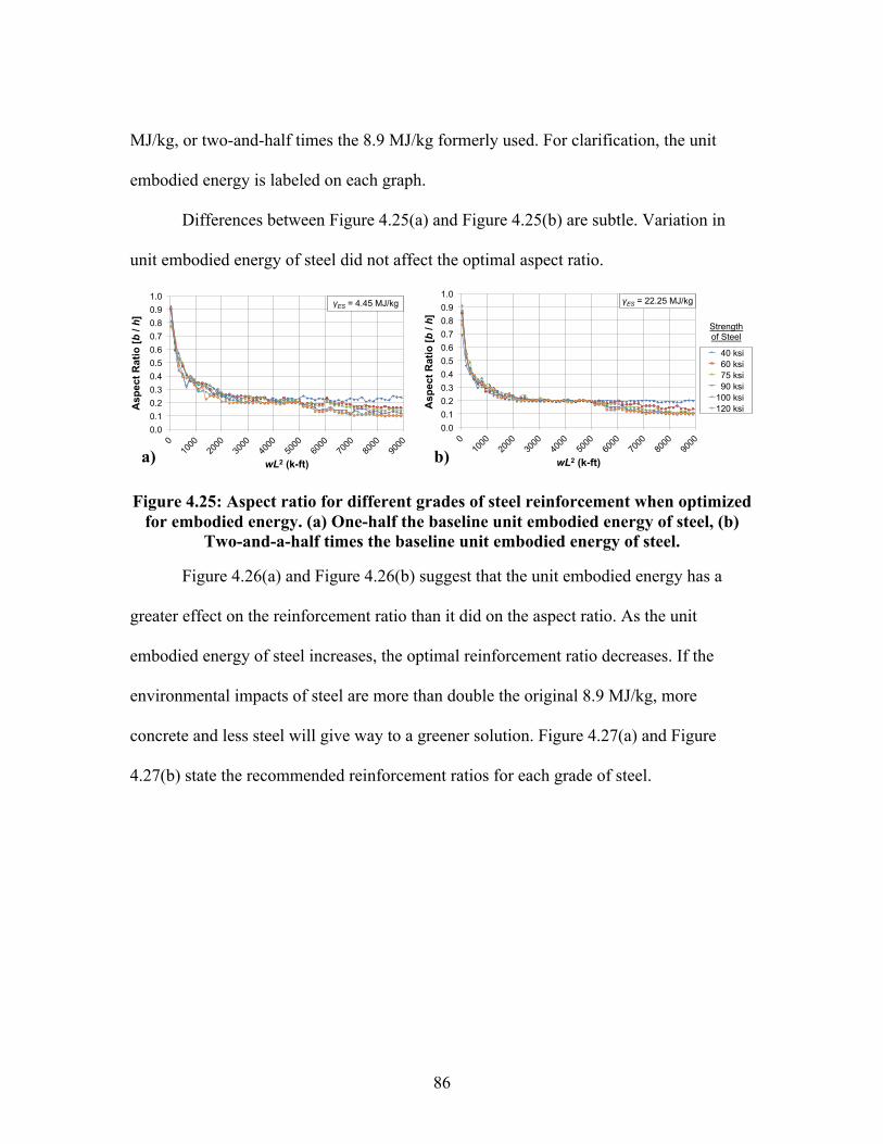
86
MJ/kg, or two-and-half times the 8.9 MJ/kg formerly used. For clarification, the unit
embodied energy is labeled on each graph.
Differences between Figure 4.25(a) and Figure 4.25(b) are subtle. Variation in
unit embodied energy of steel did not affect the optimal aspect ratio.
Figure 4.25: Aspect ratio for different grades of steel reinforcement when optimized for embodied energy. (a) One-half the baseline unit embodied energy of steel, (b)
Two-and-a-half times the baseline unit embodied energy of steel.
Figure 4.26(a) and Figure 4.26(b) suggest that the unit embodied energy has a
greater effect on the reinforcement ratio than it did on the aspect ratio. As the unit
embodied energy of steel increases, the optimal reinforcement ratio decreases. If the
environmental impacts of steel are more than double the original 8.9 MJ/kg, more
concrete and less steel will give way to a greener solution. Figure 4.27(a) and Figure
4.27(b) state the recommended reinforcement ratios for each grade of steel.
0.0 0.1 0.2 0.3 0.4 0.5 0.6 0.7 0.8 0.9 1.0
0
1000
2000
3000
4000
5000
6000
7000
8000
9000
Asp
ect R
atio
[b / h]
wL2 (k-ft)
40 ksi 60 ksi 75 ksi 90 ksi 100 ksi 120 ksi
Strength of Steel
γES = 4.45 MJ/kg
0.0 0.1 0.2 0.3 0.4 0.5 0.6 0.7 0.8 0.9 1.0
0
1000
2000
3000
4000
5000
6000
7000
8000
9000
A
spec
t Rat
io [b
/ h]
wL2 (k-ft)
40 ksi 60 ksi 75 ksi 90 ksi 100 ksi 120 ksi
Strength of Steel
γES = 22.25 MJ/kg
0.0 0.1 0.2 0.3 0.4 0.5 0.6 0.7 0.8 0.9 1.0
0
1000
2000
3000
4000
5000
6000
7000
8000
9000
A
spec
t Rat
io [b
/ h]
wL2 (k-ft)
40 ksi 60 ksi 75 ksi 90 ksi 100 ksi 120 ksi
Strength of Steel
h = ACI minimum
a) b)
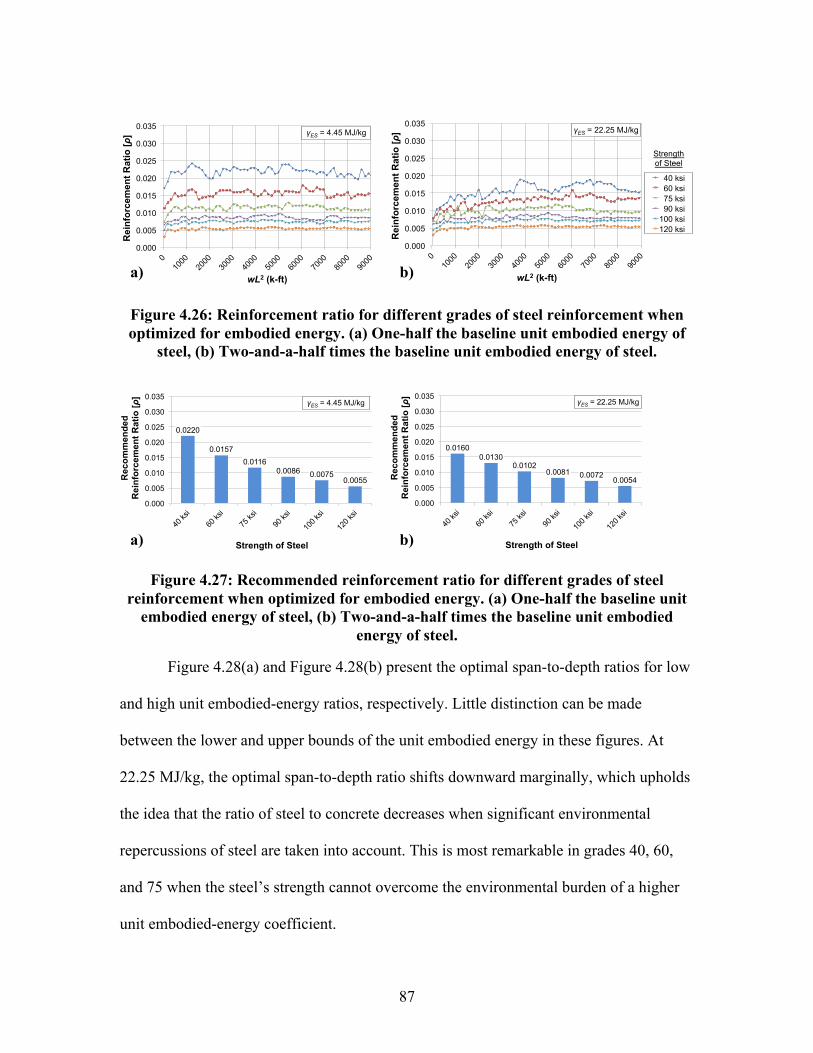
87
Figure 4.26: Reinforcement ratio for different grades of steel reinforcement when optimized for embodied energy. (a) One-half the baseline unit embodied energy of
steel, (b) Two-and-a-half times the baseline unit embodied energy of steel.
Figure 4.27: Recommended reinforcement ratio for different grades of steel reinforcement when optimized for embodied energy. (a) One-half the baseline unit
embodied energy of steel, (b) Two-and-a-half times the baseline unit embodied energy of steel.
Figure 4.28(a) and Figure 4.28(b) present the optimal span-to-depth ratios for low
and high unit embodied-energy ratios, respectively. Little distinction can be made
between the lower and upper bounds of the unit embodied energy in these figures. At
22.25 MJ/kg, the optimal span-to-depth ratio shifts downward marginally, which upholds
the idea that the ratio of steel to concrete decreases when significant environmental
repercussions of steel are taken into account. This is most remarkable in grades 40, 60,
and 75 when the steel’s strength cannot overcome the environmental burden of a higher
unit embodied-energy coefficient.
0.000
0.005
0.010
0.015
0.020
0.025
0.030
0.035
0
1000
2000
3000
4000
5000
6000
7000
8000
9000
Rei
nfor
cem
ent R
atio
[ρ]
wL2 (k-ft)
40 ksi 60 ksi 75 ksi 90 ksi 100 ksi 120 ksi
Strength of Steel
γES = 4.45 MJ/kg
0.000
0.005
0.010
0.015
0.020
0.025
0.030
0.035
0
1000
2000
3000
4000
5000
6000
7000
8000
9000
Rei
nfor
cem
ent R
atio
[ρ]
wL2 (k-ft)
40 ksi 60 ksi 75 ksi 90 ksi 100 ksi 120 ksi
Strength of Steel
γES = 22.25 MJ/kg
0.0 0.1 0.2 0.3 0.4 0.5 0.6 0.7 0.8 0.9 1.0
0
1000
2000
3000
4000
5000
6000
7000
8000
9000
Asp
ect R
atio
[b / h]
wL2 (k-ft)
40 ksi 60 ksi 75 ksi 90 ksi 100 ksi 120 ksi
Strength of Steel
h = ACI minimum
0.0220
0.0157 0.0116
0.0086 0.0075 0.0055
0.000
0.005
0.010
0.015
0.020
0.025
0.030
0.035
40 ks
i
60 ks
i
75 ks
i
90 ks
i
100 k
si
120 k
si
Rec
omm
ende
d R
einf
orce
men
t Rat
io [ρ
]
Strength of Steel
γES = 4.45 MJ/kg
0.0160 0.0130
0.0102 0.0081 0.0072
0.0054
0.000
0.005
0.010
0.015
0.020
0.025
0.030
0.035
40 ks
i
60 ks
i
75 ks
i
90 ks
i
100 k
si
120 k
si
Rec
omm
ende
d R
einf
orce
men
t Rat
io [ρ
]
Strength of Steel
γES = 22.25 MJ/kg
a) b)
a) b)

88
Figure 4.28: Span-to-depth ratio for different grades of steel reinforcement when optimized for embodied energy. (a) One-half the baseline unit embodied energy of
steel, (b) Two-and-a-half times the baseline unit embodied energy of steel.
4.3.2 Variation of Concrete Compressive Strength
4.3.2.1 Selection of Optimum Concrete Compressive Strength
Figure 4.29 and Figure 4.30 are set up in a very similar fashion to the figures in
Section 4.3.1.1 of this thesis but are optimized with regard to varying concrete
compressive strengths. Again, h has a range from L/30 to L/10 in the left column while h
is set equal to the ACI minimum beam height in the right column. For clarification, the
range of h is labeled on each graph.
In Figure 4.29 and Figure 4.30, 6,000 psi and 10,000 psi concrete are compared to
the baseline value of 4,350 psi. Like the figures in Section 4.3.1.1, these figures illustrate
when it is best to use which strength of material from an environmental perspective. Each
plot is divided into two regions, which are separated by a dashed line and labeled
appropriately.
8
10
12
14
16
18
20
22
24
26
0
1000
2000
3000
4000
5000
6000
7000
8000
9000
Spa
n-to
-Dep
th R
atio
[L /
h]
wL2 (k-ft)
40 ksi 60 ksi 75 ksi 90 ksi 100 ksi 120 ksi
Strength of Steel
γES = 4.45 MJ/kg
8
10
12
14
16
18
20
22
24
26
0
1000
2000
3000
4000
5000
6000
7000
8000
9000
Spa
n-to
-Dep
th R
atio
[L /
h]
wL2 (k-ft)
40 ksi 60 ksi 75 ksi 90 ksi 100 ksi 120 ksi
Strength of Steel
γES = 22.25 MJ/kg
0.0 0.1 0.2 0.3 0.4 0.5 0.6 0.7 0.8 0.9 1.0
0
1000
2000
3000
4000
5000
6000
7000
8000
9000
Asp
ect R
atio
[b / h]
wL2 (k-ft)
40 ksi 60 ksi 75 ksi 90 ksi 100 ksi 120 ksi
Strength of Steel
h = ACI minimum
a) b)

89
Figure 4.29: Comparison of embodied energy ratios for 4,350 psi and 6,000 psi concrete. (a) Variable span-to-depth ratio, (b) ACI minimum depth.
Figure 4.30: Comparison of embodied-energy ratios for 4,350 psi and 10,000 psi concrete. (a) Variable span-to-depth ratio, (b) ACI minimum depth.
The transition in preferability between 6,000 psi and 4,350 psi concrete lies
between a unit embodied-energy ratio of 1.00 and 1.25. This means that in many cases
6,000 psi concrete is preferable even if it has greater unit embodied energy. The figures
for 10,000 psi concrete feature very similar results to 6,000 psi concrete.
The subtle changes among different concrete strengths can be explained by the
equations used to optimize, found in Chapter 3. When the compressive strength increases,
the lower bound for the required area of steel shifts upward, which is evident in Equation
0.50
0.75
1.00
1.25
1.50
1.75
2.00
2.25
2.50
50
800
1550
23
00
3050
38
00
4550
53
00
6050
68
00
7550
83
00
9050
γ E60
00 / γ E
4350
wL2 (k-ft)
1.30-1.40 1.20-1.30 1.10-1.20 1.00-1.10 0.90-1.00 0.80-0.90 0.70-0.80 0.60-0.70
Use 4,350 psi
Use 6,000 psi
50
5250
60
00
6750
75
00
3000
37
50
2250
1500
750
4500
9000
8250
L30
< h < L10
0.50
0.75
1.00
1.25
1.50
1.75
2.00
2.25
2.50
50
800
1550
23
00
3050
38
00
4550
53
00
6050
68
00
7550
83
00
9050
γ E60
00 / γ E
4350
wL2 (k-ft)
1.30-1.40 1.20-1.30 1.10-1.20 1.00-1.10 0.90-1.00 0.80-0.90 0.70-0.80 0.60-0.70
Use 4,350 psi
Use 6,000 psi
50
5250
60
00
6750
75
00
3000
37
50
2250
1500
750
4500
9000
8250
EE6000
EE4350
h = ACI minimum
0.9 - 1.0
> 1.3 1.2 - 1.3 1.1 - 1.2 1.0 - 1.1
0.8 - 0.9 0.7 - 0.8 < 0.7
0.50
0.75
1.00
1.25
1.50
1.75
2.00
2.25
2.50
50
800
1550
23
00
3050
38
00
4550
53
00
6050
68
00
7550
83
00
9050
γ E10
000 /
γE4
350
wL2 (k-ft)
1.30-1.40 1.20-1.30 1.10-1.20 1.00-1.10 0.90-1.00 0.80-0.90 0.70-0.80 0.60-0.70
Use 4,350 psi
Use 10,000 psi
50
5250
60
00
6750
75
00
3000
37
50
2250
1500
750
4500
9000
8250
L30
< h < L10
0.50
0.75
1.00
1.25
1.50
1.75
2.00
2.25
2.50
50
800
1550
23
00
3050
38
00
4550
53
00
6050
68
00
7550
83
00
9050
γ E10
000 /
γE4
350
wL2 (k-ft)
1.30-1.40 1.20-1.30 1.10-1.20 1.00-1.10 0.90-1.00 0.80-0.90 0.70-0.80 0.60-0.70
Use 4,350 psi
Use 10,000 psi
50
5250
60
00
6750
75
00
3000
37
50
2250
1500
750
4500
9000
8250
EE10000
EE4350
h = ACI minimum
0.9 - 1.0
> 1.3 1.2 - 1.3 1.1 - 1.2 1.0 - 1.1
0.8 - 0.9 0.7 - 0.8 < 0.7
a) b)
a) b)
90
3.26. Higher-strength concrete decreases the depth of the compression block, a, given by
Equation 3.7. This increases the internal moment arm of the reinforcement and results in
a slight increase in moment capacity. Equation 3.4 demonstrates this relationship. A
greater compressive strength also directly impacts the nominal shear capacity of the
section, given in Equation 3.23. Although shear does not typically control in an optimized
section, the slight increase in the nominal moment capacity explains the subtle
differences between lines in Figure 4.29 and Figure 4.30.
4.3.2.2 Selection of Optimum Cross-Section
Figure 4.31, Figure 4.32, and Figure 4.34 exhibit results of three individual
parametric studies used to design an optimum cross-section. Figure 4.31 shows the
optimal aspect ratio for minimizing embodied energy. In Figure 4.31(a), as the moment
increases, the aspect ratio decreases sharply before leveling out. The strength of concrete
in this figure does not appear to have a significant impact on the aspect ratio; however,
higher grades of concrete do spawn designs with greater aspect ratios due to shorter
beams. While some of the curves in Figure 4.31(b) are more closely linked, the lower
grades of concrete (2,500 psi and 4,350 psi) begin to separate themselves from the others,
and are actually products of a reduced aspect ratio. Because the height of the beam is
constant and the area of the cross-section increases when lower grades of concrete are
utilized, the width of the beam must broaden.

91
Figure 4.31: Aspect ratio for different grades of concrete when optimized for embodied energy. (a) Variable span-to-depth ratio, (b) ACI minimum depth.
Figure 4.32 shows the optimal reinforcement ratio for minimizing embodied
energy. In this figure, the reinforcement ratio stays relatively constant for a given
concrete strength when the moment is greater than 500 k-ft. The bar chart in Figure 4.33
presents the recommended reinforcement ratios for different concrete grades and
emphasizes the increase of reinforcement as stronger concrete is used. Recommended
values were calculated by averaging optimum results for moments greater than 500 k-ft.
Beams designed with high-strength concrete require a smaller cross-section,
hence the uptick in the reinforcement ratio. In Figure 4.32(b), the differences between
each grade of steel are minimized. Because the height is constant, concrete strength has
less effect on optimum design, and the results are all close to the baseline of 4,350 psi.
0.0 0.1 0.2 0.3 0.4 0.5 0.6 0.7 0.8 0.9 1.0
0
1000
2000
3000
4000
5000
6000
7000
8000
9000
Asp
ect R
atio
[b / h]
wL2 (k-ft)
2,500 psi 4,350 psi 6,000 psi 8,000 psi 10,000 psi
Strength of Concrete
L30
< h < L10
0.0 0.1 0.2 0.3 0.4 0.5 0.6 0.7 0.8 0.9 1.0
0
1000
2000
3000
4000
5000
6000
7000
8000
9000
Asp
ect R
atio
[b / h]
wL2 (k-ft)
2,500 psi 4,350 psi 6,000 psi 8,000 psi 10,000 psi
Strength of Concrete
h = ACI minimum
0.000
0.005
0.010
0.015
0.020
0.025
0.030
0.035
0
1000
2000
3000
4000
5000
6000
7000
8000
9000
Rei
nfor
cem
ent R
atio
[ρ ]
wL2 (k-ft)
2,500 psi 4,350 psi 6,000 psi 8,000 psi 10,000 psi
Strength of Concrete
L30
< h < L10
a) b)
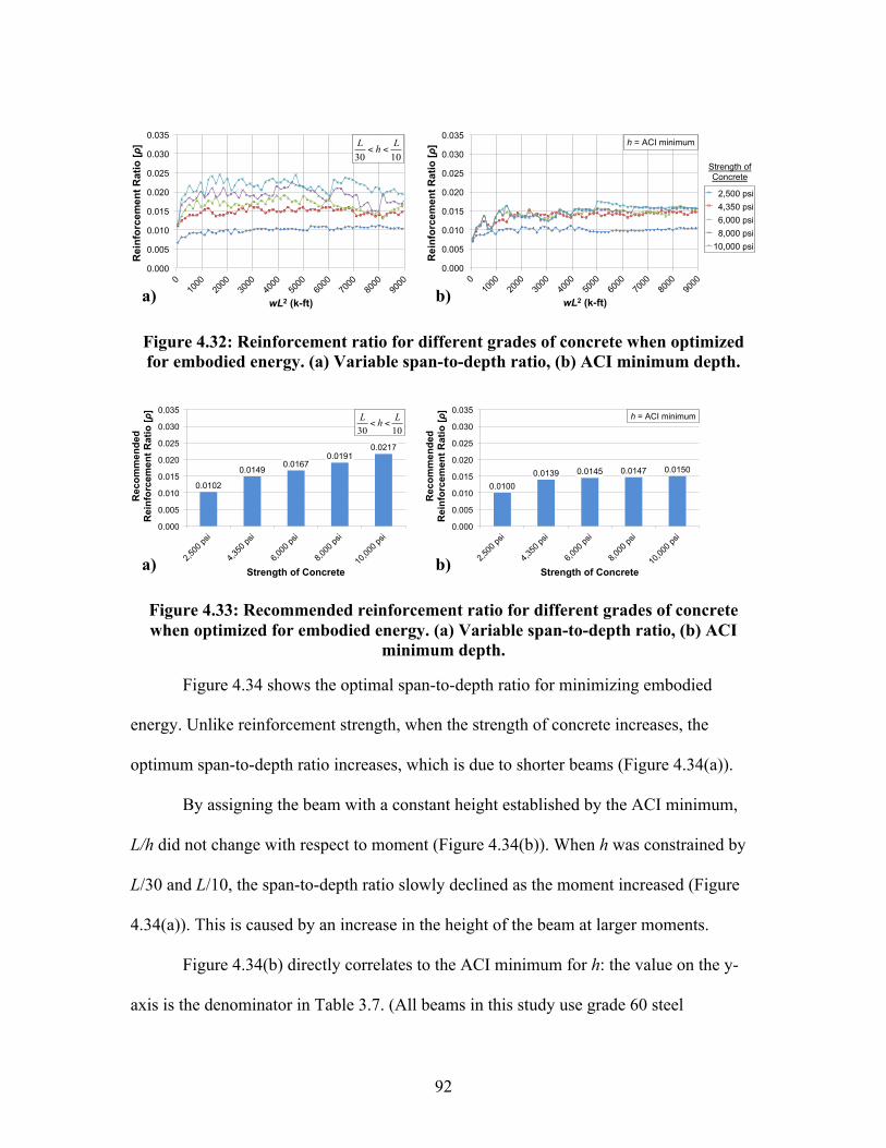
92
Figure 4.32: Reinforcement ratio for different grades of concrete when optimized for embodied energy. (a) Variable span-to-depth ratio, (b) ACI minimum depth.
Figure 4.33: Recommended reinforcement ratio for different grades of concrete when optimized for embodied energy. (a) Variable span-to-depth ratio, (b) ACI
minimum depth.
Figure 4.34 shows the optimal span-to-depth ratio for minimizing embodied
energy. Unlike reinforcement strength, when the strength of concrete increases, the
optimum span-to-depth ratio increases, which is due to shorter beams (Figure 4.34(a)).
By assigning the beam with a constant height established by the ACI minimum,
L/h did not change with respect to moment (Figure 4.34(b)). When h was constrained by
L/30 and L/10, the span-to-depth ratio slowly declined as the moment increased (Figure
4.34(a)). This is caused by an increase in the height of the beam at larger moments.
Figure 4.34(b) directly correlates to the ACI minimum for h: the value on the y-
axis is the denominator in Table 3.7. (All beams in this study use grade 60 steel
0.000
0.005
0.010
0.015
0.020
0.025
0.030
0.035
0
1000
2000
3000
4000
5000
6000
7000
8000
9000
Rei
nfor
cem
ent R
atio
[ρ]
wL2 (k-ft)
2,500 psi 4,350 psi 6,000 psi 8,000 psi 10,000 psi
Strength of Concrete
L30
< h < L10
0.000
0.005
0.010
0.015
0.020
0.025
0.030
0.035
0
1000
2000
3000
4000
5000
6000
7000
8000
9000
Rei
nfor
cem
ent R
atio
[ρ]
wL2 (k-ft)
2,500 psi 4,350 psi 6,000 psi 8,000 psi 10,000 psi
Strength of Concrete
h = ACI minimum
0.000
0.005
0.010
0.015
0.020
0.025
0.030
0.035
0
1000
2000
3000
4000
5000
6000
7000
8000
9000
Rei
nfor
cem
ent R
atio
[ρ ]
wL2 (k-ft)
2,500 psi 4,350 psi 6,000 psi 8,000 psi 10,000 psi
Strength of Concrete
L30
< h < L10
0.0102
0.0149 0.0167
0.0191 0.0217
0.000
0.005
0.010
0.015
0.020
0.025
0.030
0.035
2,500
psi
4,350
psi
6,000
psi
8,000
psi
10,00
0 psi
Rec
omm
ende
d R
einf
orce
men
t Rat
io [ρ
]
Strength of Concrete
L30
< h < L10
0.0100 0.0139 0.0145 0.0147 0.0150
0.000
0.005
0.010
0.015
0.020
0.025
0.030
0.035
2,500
psi
4,350
psi
6,000
psi
8,000
psi
10,00
0 psi
Rec
omm
ende
d R
einf
orce
men
t Rat
io [ρ
]
Strength of Concrete
h = ACI minimum
a) b)
a) b)
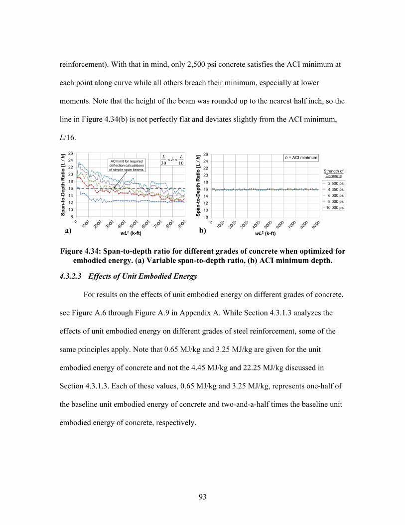
93
reinforcement). With that in mind, only 2,500 psi concrete satisfies the ACI minimum at
each point along curve while all others breach their minimum, especially at lower
moments. Note that the height of the beam was rounded up to the nearest half inch, so the
line in Figure 4.34(b) is not perfectly flat and deviates slightly from the ACI minimum,
L/16.
Figure 4.34: Span-to-depth ratio for different grades of concrete when optimized for embodied energy. (a) Variable span-to-depth ratio, (b) ACI minimum depth.
4.3.2.3 Effects of Unit Embodied Energy
For results on the effects of unit embodied energy on different grades of concrete,
see Figure A.6 through Figure A.9 in Appendix A. While Section 4.3.1.3 analyzes the
effects of unit embodied energy on different grades of steel reinforcement, some of the
same principles apply. Note that 0.65 MJ/kg and 3.25 MJ/kg are given for the unit
embodied energy of concrete and not the 4.45 MJ/kg and 22.25 MJ/kg discussed in
Section 4.3.1.3. Each of these values, 0.65 MJ/kg and 3.25 MJ/kg, represents one-half of
the baseline unit embodied energy of concrete and two-and-a-half times the baseline unit
embodied energy of concrete, respectively.
8
10
12
14
16
18
20
22
24
26
0
1000
2000
3000
4000
5000
6000
7000
8000
9000
Spa
n-to
-Dep
th R
atio
[L /
h]
wL2 (k-ft)
2,500 psi 4,350 psi 6,000 psi 8,000 psi 10,000 psi
Strength of Concrete
L30
< h < L10ACI limit for required
deflection calculations of simple span beams.
8
10
12
14
16
18
20
22
24
26
0
1000
2000
3000
4000
5000
6000
7000
8000
9000
Spa
n-to
-Dep
th R
atio
[L /
h]
wL2 (k-ft)
2,500 psi 4,350 psi 6,000 psi 8,000 psi 10,000 psi
Strength of Concrete
h = ACI minimum
0.000
0.005
0.010
0.015
0.020
0.025
0.030
0.035
0
1000
2000
3000
4000
5000
6000
7000
8000
9000
Rei
nfor
cem
ent R
atio
[ρ ]
wL2 (k-ft)
2,500 psi 4,350 psi 6,000 psi 8,000 psi 10,000 psi
Strength of Concrete
L30
< h < L10
a) b)

94
4.3.3 Variation of Concrete Unit Weight
For all studies labeled with 103 pcf, 102.5 pcf was actually used. This number
was rounded to the nearest whole number in all plots to avoid formatting issues.
4.3.3.1 Selection of Optimum Concrete Unit Weight
Figure 4.35 and Figure 4.36 are set up in a very similar fashion to the figures in
Section 4.3.1.1, but instead they are optimized with regard to varying concrete unit
weights. Again, h has a range from L/30 to L/10 in the left column while h is set equal to
the minimum beam height prescribed by ACI 318-11 in the right column. For
clarification, the range of h is labeled on each graph.
In Figure 4.35 and Figure 4.36, 90 pcf and 115 pcf concrete are compared to the
baseline value of 145 pcf. Like the figures in Section 4.3.1.1, these figures illustrate when
it is best to use which unit weight of concrete from an environmental perspective. Each
plot is divided into two regions, which are separated by a dashed line and labeled
appropriately.
In Figure 4.35(a) and Figure 4.36(a), the line indicating the transition between
preferability of concrete unit weights is practically horizontal. 90 pcf concrete is
recommended for a unit embodied energy within about 1.60 times that of 145 pcf, and
115 pcf concrete is recommended for a unit embodied energy within about 1.25 times
that of 145 pcf. Because a lighter beam produces more modest shear forces and moments,
lower unit-weight concrete is preferable to NW concrete even if LW has higher unit
embodied energy. When the height of the beam, h, is set equal to the ACI minimum in
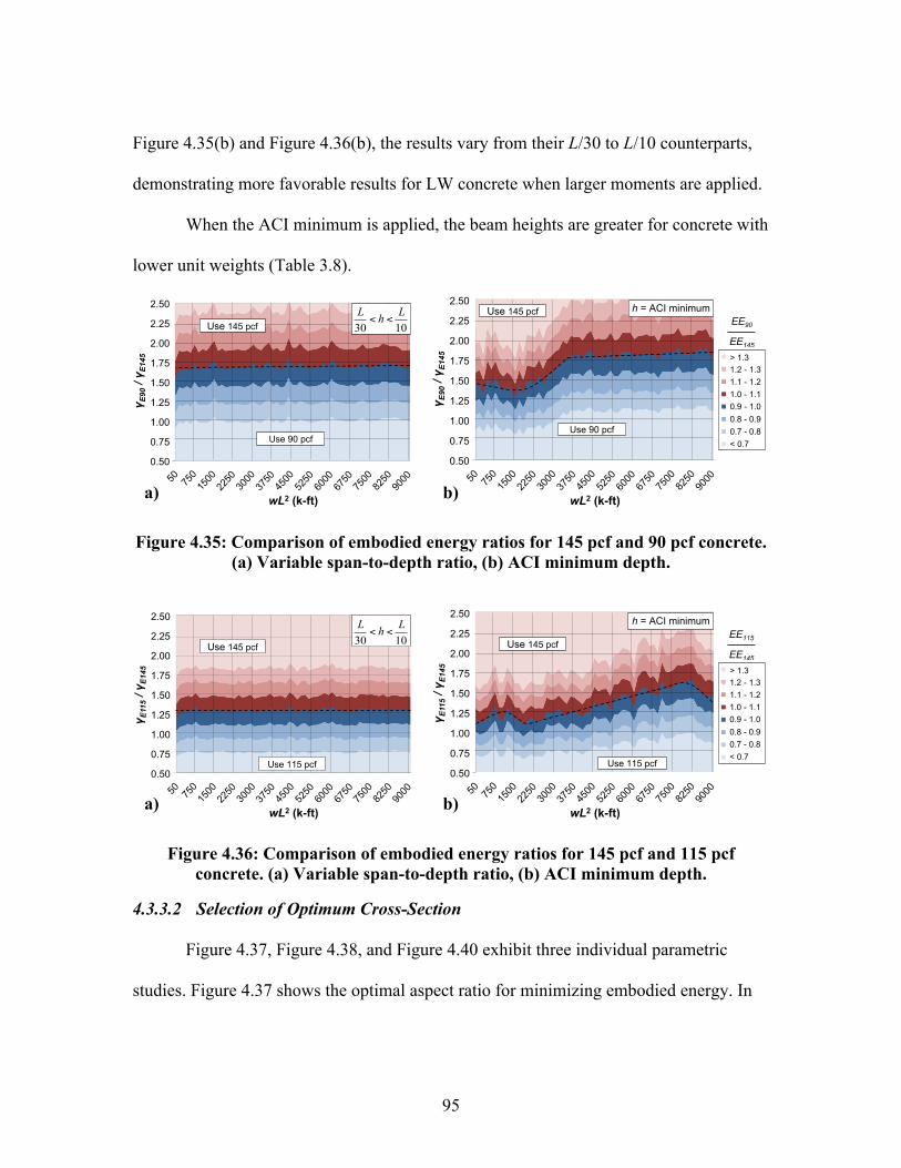
95
Figure 4.35(b) and Figure 4.36(b), the results vary from their L/30 to L/10 counterparts,
demonstrating more favorable results for LW concrete when larger moments are applied.
When the ACI minimum is applied, the beam heights are greater for concrete with
lower unit weights (Table 3.8).
Figure 4.35: Comparison of embodied energy ratios for 145 pcf and 90 pcf concrete. (a) Variable span-to-depth ratio, (b) ACI minimum depth.
Figure 4.36: Comparison of embodied energy ratios for 145 pcf and 115 pcf concrete. (a) Variable span-to-depth ratio, (b) ACI minimum depth.
4.3.3.2 Selection of Optimum Cross-Section
Figure 4.37, Figure 4.38, and Figure 4.40 exhibit three individual parametric
studies. Figure 4.37 shows the optimal aspect ratio for minimizing embodied energy. In
0.50
0.75
1.00
1.25
1.50
1.75
2.00
2.25
2.50
50
800
1550
23
00
3050
38
00
4550
53
00
6050
68
00
7550
83
00
9050
γ E90
/ γ E
145
wL2 (k-ft)
1.30-1.40 1.20-1.30 1.10-1.20 1.00-1.10 0.90-1.00 0.80-0.90 0.70-0.80 0.60-0.70
Use 145 pcf
Use 90 pcf
50
5250
60
00
6750
75
00
3000
37
50
2250
1500
750
4500
9000
8250
L30
< h < L10
0.50
0.75
1.00
1.25
1.50
1.75
2.00
2.25
2.50
50
800
1550
23
00
3050
38
00
4550
53
00
6050
68
00
7550
83
00
9050
γ E90
/ γ E
145
wL2 (k-ft)
1.30-1.40 1.20-1.30 1.10-1.20 1.00-1.10 0.90-1.00 0.80-0.90 0.70-0.80 0.60-0.70
Use 145 pcf
Use 90 pcf
50
5250
60
00
6750
75
00
3000
37
50
2250
1500
750
4500
9000
8250
EE90
EE145
0.9 - 1.0
> 1.3 1.2 - 1.3 1.1 - 1.2 1.0 - 1.1
0.8 - 0.9 0.7 - 0.8 < 0.7
h = ACI minimum
0.50
0.75
1.00
1.25
1.50
1.75
2.00
2.25
2.50
50
800
1550
23
00
3050
38
00
4550
53
00
6050
68
00
7550
83
00
9050
γ E11
5 / γ
E145
wL2 (k-ft)
1.30-1.40 1.20-1.30 1.10-1.20 1.00-1.10 0.90-1.00 0.80-0.90 0.70-0.80 0.60-0.70
Use 145 pcf
Use 115 pcf
50
5250
60
00
6750
75
00
3000
37
50
2250
1500
750
4500
9000
8250
EE115
EE145
0.9 - 1.0
> 1.3 1.2 - 1.3 1.1 - 1.2 1.0 - 1.1
0.8 - 0.9 0.7 - 0.8 < 0.7
L30
< h < L10
0.50
0.75
1.00
1.25
1.50
1.75
2.00
2.25
2.50
50
800
1550
23
00
3050
38
00
4550
53
00
6050
68
00
7550
83
00
9050
γ E11
5 / γ
E145
wL2 (k-ft)
1.30-1.40 1.20-1.30 1.10-1.20 1.00-1.10 0.90-1.00 0.80-0.90 0.70-0.80 0.60-0.70
Use 145 pcf
Use 115 pcf
50
5250
60
00
6750
75
00
3000
37
50
2250
1500
750
4500
9000
8250
EE115
EE145
0.9 - 1.0
> 1.3 1.2 - 1.3 1.1 - 1.2 1.0 - 1.1
0.8 - 0.9 0.7 - 0.8 < 0.7
h = ACI minimum
a) b)
a) b)

96
Figure 4.37(a), as the moment increases, the aspect ratio decreases sharply before
leveling out between 0.1 and 0.2. The unit weight of concrete in this figure does not have
any impact on the optimum aspect ratio. When ACI minimum thickness is regarded, the
optimum aspect ratio is increased for lighter weight concretes (Figure 4.37(b)).
Figure 4.37: Aspect ratio for different unit weights of concrete when optimized for embodied energy. (a) Variable span-to-depth ratio, (b) ACI minimum depth.
Figure 4.38 shows the optimal reinforcement ratio for minimizing embodied
energy. In this figure, the optimum reinforcement ratio stays relatively constant when the
moment is greater than 500 k-ft. The bar chart in Figure 4.39 presents the recommended
reinforcement ratios for different unit weights of concrete and emphasizes the decrease of
reinforcement as lighter concrete is used. Recommended values were calculated by
averaging optimum results for moments greater than 500 k-ft.
Optimized beams with LW concrete don’t require as much steel reinforcement as
those with NW concrete, evident in Figure 4.38 and Figure 4.39.
0.0 0.1 0.2 0.3 0.4 0.5 0.6 0.7 0.8 0.9 1.0
0
1000
2000
3000
4000
5000
6000
7000
8000
9000
Asp
ect R
atio
[b / h]
wL2 (k-ft)
90 pcf 103 pcf 115 pcf 145 pcf
Unit Weight of Concrete
L30
< h < L10
0.0 0.1 0.2 0.3 0.4 0.5 0.6 0.7 0.8 0.9 1.0
0
1000
2000
3000
4000
5000
6000
7000
8000
9000
A
spec
t Rat
io [b
/ h]
wL2 (k-ft)
90 pcf 103 pcf 115 pcf 145 pcf
Unit Weight of Concrete
h = ACI minimum
0.0 0.1 0.2 0.3 0.4 0.5 0.6 0.7 0.8 0.9 1.0
0
1000
2000
3000
4000
5000
6000
7000
8000
9000
A
spec
t Rat
io [b
/ h]
wL2 (k-ft)
90 pcf 103 pcf 115 pcf 145 pcf
Unit Weight of Concrete
γEC = 0.65 MJ/kg
a) b)

97
Figure 4.38: Reinforcement ratio for different unit weights of concrete when optimized for embodied energy. (a) Variable span-to-depth ratio, (b) ACI minimum
depth.
Figure 4.39: Recommended reinforcement ratio for different unit weights of concrete when optimized for embodied energy. (a) Variable span-to-depth ratio, (b)
ACI minimum depth.
Figure 4.40 shows the optimal span-to-depth ratio for minimizing embodied
energy. By assigning the beam with a constant height established by the ACI minimum,
L/h did not change with respect to moment (Figure 4.40(b)). When h was constrained by
L/30 and L/10, the optimum span-to-depth ratio slowly declined as the moment increased
(Figure 4.40(a)). This is caused by an increase in the height of the beam at larger
moments.
Figure 4.40(b) directly correlates to the ACI minimum for h: the value on the y-
axis is the denominator in Table 3.8. With that in mind, none of the unit weights
0.000
0.005
0.010
0.015
0.020
0.025
0.030
0.035
0
1000
2000
3000
4000
5000
6000
7000
8000
9000
Rei
nfor
cem
ent R
atio
[ρ]
wL2 (k-ft)
90 pcf 103 pcf 115 pcf 145 pcf
Unit Weight of Concrete
L30
< h < L10
0.000
0.005
0.010
0.015
0.020
0.025
0.030
0.035
0
1000
2000
3000
4000
5000
6000
7000
8000
9000
Rei
nfor
cem
ent R
atio
[ρ]
wL2 (k-ft)
90 pcf 103 pcf 115 pcf 145 pcf
Unit Weight of Concrete
h = ACI minimum
0.0 0.1 0.2 0.3 0.4 0.5 0.6 0.7 0.8 0.9 1.0
0
1000
2000
3000
4000
5000
6000
7000
8000
9000
Asp
ect R
atio
[b / h]
wL2 (k-ft)
90 pcf 103 pcf 115 pcf 145 pcf
Unit Weight of Concrete
γEC = 0.65 MJ/kg
0.0132 0.0136 0.0140 0.0149
0.000
0.005
0.010
0.015
0.020
0.025
0.030
0.035
90 p
cf
103 p
cf
115 p
cf
145 p
cf
Rec
omm
ende
d R
einf
orce
men
t Rat
io [ρ
]
Unit Weight of Concrete
L30
< h < L10
0.0106 0.0125 0.0131 0.0139
0.000
0.005
0.010
0.015
0.020
0.025
0.030
0.035
90 p
cf
103 p
cf
115 p
cf
145 p
cf
Rec
omm
ende
d R
einf
orce
men
t Rat
io [ρ
]
Unit Weight of Concrete
h = ACI minimum
a) b)
a) b)

98
considered satisfy the ACI minimum. Note that the height of the beam was rounded up to
the nearest half inch, so the lines in Figure 4.40(b) are not perfectly flat and deviate
slightly from the ACI minimum.
Figure 4.40: Span-to-depth ratio for different unit weights of concrete when
optimized for embodied energy. (a) Variable span-to-depth ratio, (b) ACI minimum depth.
4.3.3.3 Effects of Unit Embodied Energy
For results on the effects of unit embodied energy on different concrete unit
weights, see Figure A.11 through Figure A.14 in Appendix A. While Section 4.3.1.3
analyzes the effects of unit embodied energy on different grades of steel reinforcement,
some of the same principles apply. Note that 0.65 MJ/kg and 3.25 MJ/kg are given for the
unit embodied energy of concrete and not the 4.45 MJ/kg and 22.25 MJ/kg discussed in
Section 4.3.1.3. Each of these values, 0.65 MJ/kg and 3.25 MJ/kg, represent one-half of
the baseline unit embodied energy of concrete and two-and-a-half times the baseline unit
embodied energy of concrete, respectively.
8
10
12
14
16
18
20
22
24
26
0
1000
2000
3000
4000
5000
6000
7000
8000
9000
Spa
n-to
-Dep
th R
atio
[L /
h]
wL2 (k-ft)
90 pcf 103 pcf 115 pcf 145 pcf
Unit Weight of Concrete
L30
< h < L10
8
10
12
14
16
18
20
22
24
26
0
1000
2000
3000
4000
5000
6000
7000
8000
9000
Spa
n-to
-Dep
th R
atio
[L /
h]
wL2 (k-ft)
90 pcf 103 pcf 115 pcf 145 pcf
Unit Weight of Concrete
h = ACI minimum
0.0 0.1 0.2 0.3 0.4 0.5 0.6 0.7 0.8 0.9 1.0
0
1000
2000
3000
4000
5000
6000
7000
8000
9000
Asp
ect R
atio
[b / h]
wL2 (k-ft)
90 pcf 103 pcf 115 pcf 145 pcf
Unit Weight of Concrete
γEC = 0.65 MJ/kg
a) b)

99
CHAPTER FIVE
PARAMETRIC STUDIES WITH COST OPTIMIZED
5.1 Overview
In this chapter, several parametric studies have been conducted to analyze how the
flexural moment affects the design of beams optimized for cost. Parameters in these
studies include yield strength of steel reinforcement, compressive strength and unit
weight of concrete, and unit cost. In a few studies, the optimum embodied energy design
was computed to determine what effect it would have on the total cost of the section
when compared to the total cost of the optimum cost design; the same was done again,
but vice versa. When one objective function is optimized for the other, it is commonly
referred to as multiobjective optimization. Examples of this are shown in Figure 5.16
through Figure 5.19.
Explanation of Applied Moment
Consistent with Chapter 4 (see Section 4.1), changes in span length and flexural
moment were considered in all parametric studies. The applied moment, represented as
wL2, is plotted on the x-axis for each study in this chapter.
Baseline Assumptions
The baseline assumptions used in Chapter 4 are used again in this chapter. These
assumptions are discussed in detail in Section 4.1. Unless labeled otherwise, the figures
in this chapter were created using those baseline assumptions.

100
Unit Cost Values
Several sources identified the unit cost for corresponding compressive strengths
and yield strengths of concrete and steel reinforcement, respectively. The values are
given in Table 5.1 with the steel-to-concrete ratios in the rightmost column. For the
parametric studies in this section, $3.50/ft3 was used for concrete, and $245/ft3 was used
for steel reinforcement. Each of these values was taken from the 2013 edition of RS
Means after interpolating between 4,000 psi and 4,500 psi for the concrete (Waier (Ed.),
2012). Because the cost of concrete includes the cost of delivery, a ten percent reduction
was applied to account for this cost. Both of these unit costs correspond with the baseline
values. Unit cost coefficients vary for materials with different properties, but based on
limited data, constant values were used throughout this study. The values for unit
embodied energy listed in Section 4.1 were also used for multiobjective optimization in
this chapter.

101
Table 5.1: Unit cost for concrete and steel.1
Reference γ$C γ$S
γ$Sγ$C
1
Samman & Erbatur (1995) - - ≈ 20
Rajeev & Krishnamoorthy
(1998)
$20.81/ft3
(f’c = 3000 psi) $1578/ft3
(fy = 60,000 psi) 75.83
Sahab et al.2
(2001) (f’c = 5075 psi) (fy = 66,715 psi) 71.43
Paya-Zaforteza et al. (2009) (f’c = 5075 psi) (fy = 58,015 psi) 86.34
Guerra et al.2 (2011) (f’c = 4060 psi) (fy = 60,915 psi) 62.79
Yeo & Gabbai (2011)
$3.68/ft3 (f’c = 4930 psi) - -
Waier (Ed.)3
(2012) $3.78/ft3; $3.89/ft3
(f’c = 4000 psi; 4500 psi) $245/ft3
(fy = 60,000 psi) 64.85; 63
Yeo & Potra (2013)
$3.68/ft3; $3.82/ft3 (f’c = 4350 psi; 5800 psi)
$240.04/ft3
(fy = 60,915 psi) 65.21; 62.79
1Units given in SI were converted to U.S. customary 2Includes material and placement costs 3Unit cost of concrete includes delivery Methodology for presenting parametric study results
Results in this chapter are presented using the same general plot types that were
used in Chapter 4. Section 4.1 provides information on each plot type and gives an
example demonstrating how the plots can be applied in design.

102
5.2 Parametric Studies
This section contains parametric studies of cost optimization. Multiobjective
optimization of cost and embodied energy is also discussed. Results from supplementary
parametric studies on cost optimization are presented in Appendix B.
The primary purpose of the cost optimization studies conducted in this research
program is to make comparisons to the embodied energy optimization studies.
Differences between the two are dependent upon the steel-to-concrete ratio, which is 70
(Table 5.1) for the unit cost and 23.13 (Table 4.3 after multiplying each unit embodied-
energy coefficient by the respective material’s unit weight) for the unit embodied energy.
This distinction is marked by the objective functions in Equation 3.1 and Equation 3.2.
With a steel-to-concrete ratio for unit cost more than three times that of the steel-to-
concrete ratio for unit embodied energy, the parametric studies that populate this chapter
have different results than those presented in Chapter 4. Therefore, the discussion in this
chapter will concentrate on differences between cost and energy optimization results.
5.2.1 Variation of Steel Yield Strength
5.2.1.1 Selection of Optimum Steel Yield Strength
Making direct comparisons between Figure 5.1 and Figure 4.20, it’s easy to see
that when optimizing for cost, 120 ksi is more advantageous than when optimizing for
embodied energy. As stated in the previous section, the steel-to-concrete ratio for cost is
more than three times larger than it is for embodied energy; therefore, it is desirable to
reduce the amount of steel and thus reduce the overall cost. One of the leverage points of
using high-strength steel is that is reduces the demand for steel. With that knowledge, 120

103
ksi steel is of greater benefit in a cost-optimized design than in an embodied-energy
optimized design.
Figure 5.1: Comparison of cost ratios for 60 ksi and 120 ksi steel reinforcement. (a) Variable span-to-depth ratio, (b) ACI minimum depth.
5.2.1.2 Selection of Optimum Cross-Section
Figure 5.2, Figure 5.3, and Figure 5.5 can be compared to Figure 4.21, Figure
4.22, and Figure 4.24 to demonstrate this concept: in cost-optimized beams, it is better to
have less steel reinforcement and more concrete (in the form of a greater beam height)
when juxtaposed with energy-optimized beams. These relative differences between cost-
and energy-optimized beams are more pronounced for lower grades of steel.
Comparing Figure 5.2(a) and Figure 4.21(a), it can be observed that the optimum
aspect ratio is lower for cost-optimized beams than for energy-optimized beams.
However, the aspect ratio is practically identical for each of these when h is assigned the
ACI minimum since the height is restricted to one value for each yield strength (Figure
5.2(b) and Figure 4.21(b)).
0.50
0.75
1.00
1.25
1.50
1.75
2.00
2.25
2.50
50
800
1550
23
00
3050
38
00
4550
53
00
6050
68
00
7550
83
00
9050
γ $12
0 / γ
$60
wL2 (k-ft)
1.30-1.40 1.20-1.30 1.10-1.20 1.00-1.10 0.90-1.00 0.80-0.90 0.70-0.80 0.60-0.70
Use 60 ksi
50
5250
60
00
6750
75
00
3000
37
50
2250
1500
750
4500
9000
8250
Use 120 ksi
L30
< h < L10
0.50
0.75
1.00
1.25
1.50
1.75
2.00
2.25
2.50
50
800
1550
23
00
3050
38
00
4550
53
00
6050
68
00
7550
83
00
9050
γ $12
0 / γ
$60
wL2 (k-ft)
1.30-1.40 1.20-1.30 1.10-1.20 1.00-1.10 0.90-1.00 0.80-0.90 0.70-0.80 0.60-0.70
Use 60 ksi
50
5250
60
00
6750
75
00
3000
37
50
2250
1500
750
4500
9000
8250
C120
C60
0.9 - 1.0
> 1.3 1.2 - 1.3 1.1 - 1.2 1.0 - 1.1
0.8 - 0.9 0.7 - 0.8 < 0.7
h = ACI minimum
Use 120 ksi
a) b)

104
Figure 5.2: Aspect ratio for different grades of steel reinforcement when optimized for cost. (a) Variable span-to-depth ratio, (b) ACI minimum depth.
Similarly, Figure 5.3 exhibits a drop in the optimum reinforcement ratio relative
to Figure 4.22. This occurs because steel is more “expensive” from a cost perspective
than from an energy perspective, and thus cost-optimized sections have less steel
reinforcement and increased concrete. Smaller moments appear to amplify this effect
because less steel is required to support the smaller moments.
Figure 5.3: Reinforcement ratio for different grades of steel reinforcement when optimized for cost. (a) Variable span-to-depth ratio, (b) ACI minimum depth.
0.0 0.1 0.2 0.3 0.4 0.5 0.6 0.7 0.8 0.9 1.0
0
1000
2000
3000
4000
5000
6000
7000
8000
9000
Asp
ect R
atio
[b / h]
wL2 (k-ft)
40 ksi 60 ksi 75 ksi 90 ksi 100 ksi 120 ksi
Strength of Steel
L30
< h < L10
0.0 0.1 0.2 0.3 0.4 0.5 0.6 0.7 0.8 0.9 1.0
0
1000
2000
3000
4000
5000
6000
7000
8000
9000
Asp
ect R
atio
[b / h]
wL2 (k-ft)
40 ksi 60 ksi 75 ksi 90 ksi 100 ksi 120 ksi
Strength of Steel
h = ACI minimum
0.0 0.1 0.2 0.3 0.4 0.5 0.6 0.7 0.8 0.9 1.0
0
1000
2000
3000
4000
5000
6000
7000
8000
9000
Asp
ect R
atio
[b / h]
wL2 (k-ft)
40 ksi 60 ksi 75 ksi 90 ksi 100 ksi 120 ksi
Strength of Steel
h = ACI minimum
0.000
0.005
0.010
0.015
0.020
0.025
0.030
0.035
0
1000
2000
3000
4000
5000
6000
7000
8000
9000
Rei
nfor
cem
ent R
atio
[ρ]
wL2 (k-ft)
40 ksi 60 ksi 75 ksi 90 ksi 100 ksi 120 ksi
Strength of Steel
L30
< h < L10
0.000
0.005
0.010
0.015
0.020
0.025
0.030
0.035
0
1000
2000
3000
4000
5000
6000
7000
8000
9000
Rei
nfor
cem
ent R
atio
[ρ]
wL2 (k-ft)
40 ksi 60 ksi 75 ksi 90 ksi 100 ksi 120 ksi
Strength of Steel
h = ACI minimum
0.0 0.1 0.2 0.3 0.4 0.5 0.6 0.7 0.8 0.9 1.0
0
1000
2000
3000
4000
5000
6000
7000
8000
9000
Asp
ect R
atio
[b / h]
wL2 (k-ft)
40 ksi 60 ksi 75 ksi 90 ksi 100 ksi 120 ksi
Strength of Steel
h = ACI minimum
a) b)
a) b)
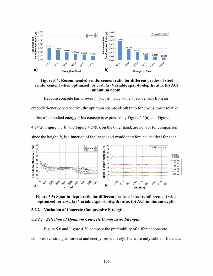
105
Figure 5.4: Recommended reinforcement ratio for different grades of steel reinforcement when optimized for cost. (a) Variable span-to-depth ratio, (b) ACI
minimum depth.
Because concrete has a lower impact from a cost perspective than from an
embodied-energy perspective, the optimum span-to-depth ratio for cost is lower relative
to that of embodied energy. This concept is expressed by Figure 5.5(a) and Figure
4.24(a). Figure 5.5(b) and Figure 4.24(b), on the other hand, are not apt for comparison
since the height, h, is a function of the length and would therefore be identical for each.
Figure 5.5: Span-to-depth ratio for different grades of steel reinforcement when optimized for cost. (a) Variable span-to-depth ratio, (b) ACI minimum depth.
5.2.2 Variation of Concrete Compressive Strength
5.2.2.1 Selection of Optimum Concrete Compressive Strength
Figure 5.6 and Figure 4.30 compare the preferability of different concrete
compressive strengths for cost and energy, respectively. There are only subtle differences
0.0153 0.0124
0.0099 0.0080 0.0070 0.0054
0.000
0.005
0.010
0.015
0.020
0.025
0.030
0.035
40 ks
i
60 ks
i
75 ks
i
90 ks
i
100 k
si
120 k
si
Rec
omm
ende
d R
einf
orce
men
t Rat
io [ρ
]
Strength of Steel
L30
< h < L10
0.0239
0.0138 0.0101
0.0061 0.0046 0.0033
0.000
0.005
0.010
0.015
0.020
0.025
0.030
0.035
40 ks
i
60 ks
i
75 ks
i
90 ks
i
100 k
si
120 k
si
Rec
omm
ende
d R
einf
orce
men
t Rat
io [ρ
]
Strength of Steel
h = ACI minimum
8
10
12
14
16
18
20
22
24
26
0
1000
2000
3000
4000
5000
6000
7000
8000
9000
Spa
n-to
-Dep
th R
atio
[L /
h]
wL2 (k-ft)
40 ksi 60 ksi 75 ksi 90 ksi 100 ksi 120 ksi
Strength of Steel
L30
< h < L10
8
10
12
14
16
18
20
22
24
26
0
1000
2000
3000
4000
5000
6000
7000
8000
9000
Spa
n-to
-Dep
th R
atio
[L /
h]
wL2 (k-ft)
40 ksi 60 ksi 75 ksi 90 ksi 100 ksi 120 ksi
Strength of Steel
h = ACI minimum
0.0 0.1 0.2 0.3 0.4 0.5 0.6 0.7 0.8 0.9 1.0
0
1000
2000
3000
4000
5000
6000
7000
8000
9000
Asp
ect R
atio
[b / h]
wL2 (k-ft)
40 ksi 60 ksi 75 ksi 90 ksi 100 ksi 120 ksi
Strength of Steel
h = ACI minimum
a) b)
a) b)

106
between these two figures, suggesting that preferable compressive strength does not vary
significantly between cost- and energy-optimized beams. However, stronger concrete can
increase the nominal moment capacity of the section, which may produce a design with
marginally less steel. This can be observed in Figure 5.6(a) where the dashed line shifts
slightly downward relative to Figure 4.30(a). Though it may be counterintuitive at first
glance, the steel-to-concrete ratio is actually decreasing as one travels up the y-axis,
opposite of that in Figure 5.1. This is because the unit cost of the concrete is being
multiplied by a factor ranging from 0.5 to 2.5, so at 2.5, the steel-to-concrete ratio is less
than at 0.5. Therefore, high-strength concrete produces designs with less reinforcement.
Figure 5.6: Comparison of cost ratios for 4,350 psi and 10,000 psi concrete. (a) Variable span-to-depth ratio, (b) ACI minimum depth.
0.50
0.75
1.00
1.25
1.50
1.75
2.00
2.25
2.50
50
800
1550
23
00
3050
38
00
4550
53
00
6050
68
00
7550
83
00
9050
γ $10
000 /
γ$4
350
wL2 (k-ft)
1.30-1.40 1.20-1.30 1.10-1.20 1.00-1.10 0.90-1.00 0.80-0.90 0.70-0.80 0.60-0.70
Use 4,350 psi
50
5250
60
00
6750
75
00
3000
37
50
2250
1500
750
4500
9000
8250
C10000
C4350
0.9 - 1.0
> 1.3 1.2 - 1.3 1.1 - 1.2 1.0 - 1.1
0.8 - 0.9 0.7 - 0.8 < 0.7 Use 10,000 psi
L30
< h < L10
0.50
0.75
1.00
1.25
1.50
1.75
2.00
2.25
2.50
50
800
1550
23
00
3050
38
00
4550
53
00
6050
68
00
7550
83
00
9050
γ $10
000 /
γ$4
350
wL2 (k-ft)
1.30-1.40 1.20-1.30 1.10-1.20 1.00-1.10 0.90-1.00 0.80-0.90 0.70-0.80 0.60-0.70
Use 4,350 psi
50
5250
60
00
6750
75
00
3000
37
50
2250
1500
750
4500
9000
8250
C10000
C4350
0.9 - 1.0
> 1.3 1.2 - 1.3 1.1 - 1.2 1.0 - 1.1
0.8 - 0.9 0.7 - 0.8 < 0.7 Use 10,000 psi
h = ACI minimum
a) b)

107
5.2.2.2 Selection of Optimum Cross-Section
Figure 5.7, Figure 5.8, and Figure 5.10 show the cost-optimum aspect,
reinforcement, and span-to-depth ratios, respectively, for varying strengths of concrete.
When compared to the energy-optimized results (Section 4.3.2.2), the cost-optimum
ratios have more concrete and less steel. As discussed in Section 5.2.1.2, this occurs
because steel is more “expensive” than concrete from a cost perspective than from an
energy perspective. However, the relative differences between cost- and energy-
optimized beams are more pronounced for higher-strength concrete.
Figure 5.7: Aspect ratio for different grades of concrete when optimized for cost. (a) Variable span-to-depth ratio, (b) ACI minimum depth.
Figure 5.8: Reinforcement ratio for different grades of concrete when optimized for cost. (a) Variable span-to-depth ratio, (b) ACI minimum depth.
0.0 0.1 0.2 0.3 0.4 0.5 0.6 0.7 0.8 0.9 1.0
0
1000
2000
3000
4000
5000
6000
7000
8000
9000
Asp
ect R
atio
[b / h]
wL2 (k-ft)
2,500 psi 4,350 psi 6,000 psi 8,000 psi 10,000 psi
Strength of Concrete
L30
< h < L10
0.0 0.1 0.2 0.3 0.4 0.5 0.6 0.7 0.8 0.9 1.0
0
1000
2000
3000
4000
5000
6000
7000
8000
9000
Asp
ect R
atio
[b / h]
wL2 (k-ft)
2,500 psi 4,350 psi 6,000 psi 8,000 psi 10,000 psi
Strength of Concrete
h = ACI minimum
0.000
0.005
0.010
0.015
0.020
0.025
0.030
0.035
0
1000
2000
3000
4000
5000
6000
7000
8000
9000
Rei
nfor
cem
ent R
atio
[ρ ]
wL2 (k-ft)
2,500 psi 4,350 psi 6,000 psi 8,000 psi 10,000 psi
Strength of Concrete
L30
< h < L10
0.000
0.005
0.010
0.015
0.020
0.025
0.030
0.035
0
1000
2000
3000
4000
5000
6000
7000
8000
9000
Rei
nfor
cem
ent R
atio
[ρ]
wL2 (k-ft)
2,500 psi 4,350 psi 6,000 psi 8,000 psi 10,000 psi
Strength of Concrete
L30
< h < L10
0.000
0.005
0.010
0.015
0.020
0.025
0.030
0.035
0
1000
2000
3000
4000
5000
6000
7000
8000
9000
Rei
nfor
cem
ent R
atio
[ρ]
wL2 (k-ft)
2,500 psi 4,350 psi 6,000 psi 8,000 psi 10,000 psi
Strength of Concrete
h = ACI minimum
0.000
0.005
0.010
0.015
0.020
0.025
0.030
0.035
0
1000
2000
3000
4000
5000
6000
7000
8000
9000
Rei
nfor
cem
ent R
atio
[ρ ]
wL2 (k-ft)
2,500 psi 4,350 psi 6,000 psi 8,000 psi 10,000 psi
Strength of Concrete
L30
< h < L10
a) b)
a) b)

108
Figure 5.9: Recommended reinforcement ratio for different grades of concrete when optimized for cost. (a) Variable span-to-depth ratio, (b) ACI minimum depth.
Figure 5.10: Span-to-depth ratio for different grades of concrete when optimized for cost. (a) Variable span-to-depth ratio, (b) ACI minimum depth.
5.2.3 Variation of Concrete Unit Weight
5.2.3.1 Selection of Optimum Concrete Unit Weight
Cost and energy comparisons of optimum concrete unit weight can be made using
Figure 5.11 and Figure 4.35, respectively. Although the trends are similar in both figures,
lightweight concrete is slightly more beneficial from a cost perspective than for energy.
This is because LW concrete reduces the load demand, and consequently the required
reinforcement, relative to NW concrete. Reduced steel quantity has a greater effect on
cost than on embodied energy. Just like Figure 5.6, as one moves upward along the y-
axis, the steel-to-concrete ratio is decreasing in Figure 5.11. So because a lighter beam
0.0096 0.0124 0.0130 0.0134 0.0135
0.000
0.005
0.010
0.015
0.020
0.025
0.030
0.035
2,500
psi
4,350
psi
6,000
psi
8,000
psi
10,00
0 psi
Rec
omm
ende
d R
einf
orce
men
t Rat
io [ρ
]
Strength of Concrete
L30
< h < L10
0.0100 0.0138 0.0142 0.0142 0.0142
0.000
0.005
0.010
0.015
0.020
0.025
0.030
0.035
2,500
psi
4,350
psi
6,000
psi
8,000
psi
10,00
0 psi
Rec
omm
ende
d R
einf
orce
men
t Rat
io [ρ
]
Strength of Concrete
h = ACI minimum
8
10
12
14
16
18
20
22
24
26
0
1000
2000
3000
4000
5000
6000
7000
8000
9000
Spa
n-to
-Dep
th R
atio
[L /
h]
wL2 (k-ft)
2,500 psi 4,350 psi 6,000 psi 8,000 psi 10,000 psi
Strength of Concrete
L30
< h < L10ACI limit for required
deflection calculations of simple span beams.
8
10
12
14
16
18
20
22
24
26
0
1000
2000
3000
4000
5000
6000
7000
8000
9000
Spa
n-to
-Dep
th R
atio
[L /
h]
wL2 (k-ft)
2,500 psi 4,350 psi 6,000 psi 8,000 psi 10,000 psi
Strength of Concrete
h = ACI minimum
0.000
0.005
0.010
0.015
0.020
0.025
0.030
0.035
0
1000
2000
3000
4000
5000
6000
7000
8000
9000
Rei
nfor
cem
ent R
atio
[ρ ]
wL2 (k-ft)
2,500 psi 4,350 psi 6,000 psi 8,000 psi 10,000 psi
Strength of Concrete
L30
< h < L10
a) b)
a) b)

109
lessens the factored shear and moment in that member and consequently lowers the
demand for steel, the dashed line in Figure 5.11 shifts downward relative to Figure 4.35.
Figure 5.11: Comparison of cost ratios for 145 pcf and 90 pcf concrete. (a) Variable span-to-depth ratio, (b) ACI minimum depth.
5.2.3.2 Selection of Optimum Cross-Section
Figure 5.12, Figure 5.13, and Figure 5.15 show the cost-optimum aspect,
reinforcement, and span-to-depth ratios, respectively, for varying concrete unit weight.
When compared to the studies of embodied energy, each of these figures hinges on the
same basic principles discussed in Section 5.2.1.2. However, the various unit weights
have little to no bearing on the relative differences between cost- and energy-optimized
beams.
0.50
0.75
1.00
1.25
1.50
1.75
2.00
2.25
2.50
50
800
1550
23
00
3050
38
00
4550
53
00
6050
68
00
7550
83
00
9050
γ $90
/ γ $
145
wL2 (k-ft)
1.30-1.40 1.20-1.30 1.10-1.20 1.00-1.10 0.90-1.00 0.80-0.90 0.70-0.80 0.60-0.70
Use 145 pcf
50
5250
60
00
6750
75
00
3000
37
50
2250
1500
750
4500
9000
8250
C90
C145
0.9 - 1.0
> 1.3 1.2 - 1.3 1.1 - 1.2 1.0 - 1.1
0.8 - 0.9 0.7 - 0.8 < 0.7 Use 90 pcf
L30
< h < L10
0.50
0.75
1.00
1.25
1.50
1.75
2.00
2.25
2.50
50
800
1550
23
00
3050
38
00
4550
53
00
6050
68
00
7550
83
00
9050
γ $90
/ γ $
145
wL2 (k-ft)
1.30-1.40 1.20-1.30 1.10-1.20 1.00-1.10 0.90-1.00 0.80-0.90 0.70-0.80 0.60-0.70
Use 145 pcf
50
5250
60
00
6750
75
00
3000
37
50
2250
1500
750
4500
9000
8250
C90
C145
0.9 - 1.0
> 1.3 1.2 - 1.3 1.1 - 1.2 1.0 - 1.1
0.8 - 0.9 0.7 - 0.8 < 0.7
Use 90 pcf
h = ACI minimum
a) b)

110
Figure 5.12: Aspect ratio for different unit weights of concrete when optimized for cost. (a) Variable span-to-depth ratio, (b) ACI minimum depth.
Figure 5.13: Reinforcement ratio for different unit weights of concrete when optimized for cost. (a) Variable span-to-depth ratio, (b) ACI minimum depth.
Figure 5.14: Recommended reinforcement ratio for different unit weights of concrete when optimized for cost. (a) Variable span-to-depth ratio, (b) ACI
minimum depth.
0.0 0.1 0.2 0.3 0.4 0.5 0.6 0.7 0.8 0.9 1.0
0
1000
2000
3000
4000
5000
6000
7000
8000
9000
Asp
ect R
atio
[b / h]
wL2 (k-ft)
90 pcf 103 pcf 115 pcf 145 pcf
Unit Weight of Concrete
L30
< h < L10
0.0 0.1 0.2 0.3 0.4 0.5 0.6 0.7 0.8 0.9 1.0
0
1000
2000
3000
4000
5000
6000
7000
8000
9000
Asp
ect R
atio
[b / h]
wL2 (k-ft)
90 pcf 103 pcf 115 pcf 145 pcf
Unit Weight of Concrete
h = ACI minimum
0.0 0.1 0.2 0.3 0.4 0.5 0.6 0.7 0.8 0.9 1.0
0
1000
2000
3000
4000
5000
6000
7000
8000
9000
Asp
ect R
atio
[b / h]
wL2 (k-ft)
90 pcf 103 pcf 115 pcf 145 pcf
Unit Weight of Concrete
γEC = 0.65 MJ/kg
0.000
0.005
0.010
0.015
0.020
0.025
0.030
0.035
0
1000
2000
3000
4000
5000
6000
7000
8000
9000
Rei
nfor
cem
ent R
atio
[ρ]
wL2 (k-ft)
90 pcf 103 pcf 115 pcf 145 pcf
Unit Weight of Concrete
L30
< h < L10
0.000
0.005
0.010
0.015
0.020
0.025
0.030
0.035
0
1000
2000
3000
4000
5000
6000
7000
8000
9000
Rei
nfor
cem
ent R
atio
[ρ]
wL2 (k-ft)
90 pcf 103 pcf 115 pcf 145 pcf
Unit Weight of Concrete
h = ACI minimum
0.0 0.1 0.2 0.3 0.4 0.5 0.6 0.7 0.8 0.9 1.0
0
1000
2000
3000
4000
5000
6000
7000
8000
9000
Asp
ect R
atio
[b / h]
wL2 (k-ft)
90 pcf 103 pcf 115 pcf 145 pcf
Unit Weight of Concrete
γEC = 0.65 MJ/kg
0.0116 0.0118 0.0119 0.0124
0.000
0.005
0.010
0.015
0.020
0.025
0.030
0.035
90 pc
f
103 p
cf
115 p
cf
145 p
cf
Rec
omm
ende
d R
einf
orce
men
t Rat
io [ρ
]
Unit Weight of Concrete
L30
< h < L10
0.0103 0.0122 0.0129 0.0138
0.000
0.005
0.010
0.015
0.020
0.025
0.030
0.035
90 pc
f
103 p
cf
115 p
cf
145 p
cf
Rec
omm
ende
d R
einf
orce
men
t Rat
io [ρ
]
Unit Weight of Concrete
h = ACI minimum
a) b)
a) b)
a) b)

111
Figure 5.15: Span-to-depth ratio for different unit weights of concrete when optimized for cost. (a) Variable span-to-depth ratio, (b) ACI minimum depth.
5.2.4 Cost and Embodied Energy Multiobjective Optimization
Figure 5.16 and Figure 5.18 show that the relationship between optimized cost
and optimized embodied energy are strongly correlated. Results in these figures are
consistent with the findings from Paya-Zaforteza et al. (2009) as presented in Figure 2.5.
These researchers found a strong correlation between optimized CO2 emissions and
optimized cost. Figure 5.16 and Figure 5.18 also show that the total embodied energy and
total cost have a positive linear correlation with the flexural moment. It is apparent that
limiting the height of the beam to the ACI minimum lends itself to an enlarged total
embodied energy and total cost.
While the differences between the embodied-energy optimized design and the
cost-optimized design are not pronounced in Figure 5.16 and Figure 5.18, Figure 5.17
and Figure 5.19 give a clear indication of the influence of simultaneous optimization.
Values presented in Figure 5.17 are the average total embodied energy from the top ten
cost-optimum designs divided by the average total embodied energy from the top ten
embodied-energy-optimum designs. Thus, the percentage of additional energy used could
be determined for cost-optimized design when compared to energy-optimized designs.
8
10
12
14
16
18
20
22
24
26
0
1000
2000
3000
4000
5000
6000
7000
8000
9000
Spa
n-to
-Dep
th R
atio
[L /
h]
wL2 (k-ft)
90 pcf 103 pcf 115 pcf 145 pcf
Unit Weight of Concrete
L30
< h < L10
8
10
12
14
16
18
20
22
24
26
0
1000
2000
3000
4000
5000
6000
7000
8000
9000
Spa
n-to
-Dep
th R
atio
[L /
h]
wL2 (k-ft)
90 pcf 103 pcf 115 pcf 145 pcf
Unit Weight of Concrete
h = ACI minimum
0.0 0.1 0.2 0.3 0.4 0.5 0.6 0.7 0.8 0.9 1.0
0
1000
2000
3000
4000
5000
6000
7000
8000
9000
Asp
ect R
atio
[b / h]
wL2 (k-ft)
90 pcf 103 pcf 115 pcf 145 pcf
Unit Weight of Concrete
γEC = 0.65 MJ/kg
a) b)

112
Between five and ten percent more energy was used for cost-optimized short-span beams,
but that difference in energy use approaches zero as the moment grows in magnitude.
This phenomenon can be explained by Figure 5.16(a), where the two lines run parallel to
each other; the difference between the two does not change a great deal, but larger
numbers are being divided and therefore smaller percentages are occurring. When the
ACI minimum is applied, the two lines in Figure 5.16(b) are virtually equal to each other,
hence the horizontal line running throughout Figure 5.17(b).
Figure 5.18 and Figure 5.19 feature the cost when optimized for total embodied
energy and total cost. The figures demonstrate very similar findings to Figure 5.16 and
Figure 5.17, albeit with a smaller percent difference between the two.
Results from the multiobjective optimization show that cost-optimized beams
have up to 10% more embodied energy than do energy-optimized beams but are up to 5%
cheaper than energy-optimized beams (Figure 5.17(a) and Figure 5.19(a)).

113
Figure 5.16: Total embodied energy of the beam when optimized for embodied energy and for cost. (a) Variable span-to-depth ratio, (b) ACI minimum depth.
Figure 5.17: Total embodied energy of the cost-optimized design divided by the total embodied energy of the embodied energy-optimized design. (a) Variable span-to-
depth ratio, (b) ACI minimum depth.
Figure 5.18: Total cost of the beam when optimized for embodied energy and for cost. (a) Variable span-to-depth ratio, (b) ACI minimum depth.
0 5,000
10,000 15,000 20,000 25,000 30,000 35,000 40,000 45,000 50,000
0 10
00
2000
30
00
4000
50
00
6000
70
00
8000
90
00
Tota
l Em
bodi
ed E
nerg
y (M
J)
wL2 (k-ft)
EE Optimized
Cost Optimized
L30
< h < L10
0 5,000
10,000 15,000 20,000 25,000 30,000 35,000 40,000 45,000 50,000
0 10
00
2000
30
00
4000
50
00
6000
70
00
8000
90
00
Tota
l Em
bodi
ed E
nerg
y (M
J)
wL2 (k-ft)
EE Optimized
Cost Optimized
h = ACI minimum
0.85
0.90
0.95
1.00
1.05
1.10
1.15
0 10
00
2000
30
00
4000
50
00
6000
70
00
8000
90
00
EEC
ost_
Opt
/ EE
EE_O
pt
wL2 (k-ft)
L30
< h < L10
0.85
0.90
0.95
1.00
1.05
1.10
1.15
0 10
00
2000
30
00
4000
50
00
6000
70
00
8000
90
00
EEC
ost_
Opt
/ EE
EE_O
pt
wL2 (k-ft)
h = ACI minimum
0
500
1,000
1,500
2,000
2,500
3,000
3,500
0 10
00
2000
30
00
4000
50
00
6000
70
00
8000
90
00
Tota
l Cos
t ($)
wL2 (k-ft)
EE Optimized
Cost Optimized
L30
< h < L10
0
500
1,000
1,500
2,000
2,500
3,000
3,500
0 10
00
2000
30
00
4000
50
00
6000
70
00
8000
90
00
Tota
l Cos
t ($)
wL2 (k-ft)
EE Optimized
Cost Optimized
h = ACI minimum
a) b)
a) b)
a) b)

114
Figure 5.19: Total cost of the embodied energy-optimized design divided by the total cost of the cost-optimized design. (a) Variable span-to-depth ratio, (b) ACI
minimum depth.
0.85
0.90
0.95
1.00
1.05
1.10
1.15
0 10
00
2000
30
00
4000
50
00
6000
70
00
8000
90
00
Cos
t EE_
Opt
/ C
ost C
ost_
Opt
wL2 (k-ft)
L30
< h < L10
0.85
0.90
0.95
1.00
1.05
1.10
1.15
0 10
00
2000
30
00
4000
50
00
6000
70
00
8000
90
00
Cos
t EE_
Opt
/ C
ost C
ost_
Opt
wL2 (k-ft)
h = ACI minimum
a) b)

115
CHAPTER SIX
SUMMARY AND CONCLUSIONS
6.1 Summary and Conclusions
A methodology for optimizing RC beams for minimized cost and/or embodied
energy was presented, which utilized concepts of LCA, optimization, and reinforced-
concrete analysis. The methodology can be applied to determine environmental or
economic preferability of different materials used in RC beams. Once materials are
selected, the methodology can also be used to design RC sections for minimized
economic cost, environmental cost, or both. The methodology was created by considering
a wide range of unit cost or unit embodied-energy coefficients to the optimization
process.
After developing parametric studies for aspect, reinforcement, and span-to-depth
ratios, several overarching trends were observed. The foremost observation was that the
optimal results were highly sensitive to the problem constraints. For example, by
constraining the span-to-depth ratio to one constant value prescribed by ACI 318-11 for
omitting deflection calculations, significant changes in material preferability and
optimum cross-section were observed when compared to an unconstrained span-to-depth
ratio.
In studies evaluating the reinforcement ratio, it was observed that the optimal ratio
did not vary significantly with the flexural moment. Given this fairly constant trend, it
was reasonable to average the values together for a given reinforcement yield strength
and provide that as the recommended reinforcement ratio. Au contraire, the optimal

116
aspect and span-to-depth ratios were not constant for changes in moment. The aspect
ratio had a negative exponential relationship with the flexural moment, dipping down
sharply before leveling off at larger moments. The span-to-depth ratio decreased at a
fairly constant rate as the flexural moment increased. These trends were observed
generally even as material property parameters were changed.
Three different material properties were considered in the optimization program:
reinforcement yield strength, concrete compressive strength, and concrete unit weight. As
the strength of the steel reinforcement increased, the optimum designs had less steel.
Similarly, as the weight of the concrete decreased, the optimum designs had less steel.
The strength of the concrete had a much less significant role on the influence of the
optimal design.
The ratio of steel-to-concrete cost is greater than the ratio of steel-to-concrete
embodied energy, which means that steel is more “expensive” from a cost perspective
than from an energy perspective. This difference results in cost-optimum designs having
less steel and more concrete; knowing this and the aforementioned effects of different
materials, high-strength steel and LW concrete have a greater impact on the minimization
of cost than they do on the minimization of energy. On the other hand, high-strength
concrete makes little difference between the optimization of cost and energy.
Multiobjective optimization results of cost and energy were consistent with
previous studies that also showed strong correlation between cost and energy optimum
designs. Total cost and total embodied energy are also proportional to the flexural
moment. Multiobjective optimization suggests that cost-optimized beams have up to 10%

117
more embodied energy than do energy-optimized beams but are up to 5% cheaper than
energy-optimized beams.
6.2 Recommendations for Future Work
Throughout this study, only simply supported rectangular RC beams were
considered. However, the types of problems that could be explored are practically
limitless. Other applications to be examined include different boundary conditions,
different types of structural systems (as opposed to single components), different
environmental metrics, and prestressed concrete.
While simply supported beams are common in design analysis, other types of
boundary conditions include fixed-fixed, cantilever, and continuous beams. Changing the
support conditions produces different shear and moments; therefore, the design criteria
for meeting flexural and shear constraints would change in response to these modified
values.
There is value in analyzing only one structural component as was done in this
study; designers can break down the design of optimal members into an isolated element,
which is not so easily accomplished in more complex structural systems. However,
structural systems provide a more realistic representation of how individual members are
behaving in a larger scheme, thus supplying the engineer with more applicable design
criteria. Thus, a natural extension of this research would be optimization of RC systems.
Embodied energy and carbon dioxide emissions are just two metrics utilized to
examine the environmental impacts of reinforced concrete. Both of these metrics are
associated with the impacts of climate change and are closely linked to one another.

118
Other metrics used in the life cycle inventory of construction materials include mineral
depletion, land use, and human toxicity. These metrics should also be considered in
future analyses.
Prestressed concrete has many beneficial applications and can be used to generate
more efficient members. While prestressed concrete design is more involved, it may help
advance the capacity of structural concrete optimization. Because concrete is used in
many bridges, studies pertaining to prestressed concrete should also include durability
and degradation as design criteria.
Integrated design is a collaborative effort that incorporates the multiple parties
responsible for design, construction, and maintenance of a building. These groups include
mechanical, electrical, and structural engineers, as well as architects and contractors. The
integrated design process helps to promote holistic design, which could enhance the
optimization of structural concrete systems from a practical standpoint.
Finally, it is suggested that future research in this area should include evaluation
of additional concrete and reinforcement materials. Low-carbon cement is a technology
that has promise for reducing the environmental footprint of the RC structures. The
methodology developed in this thesis would be useful in evaluating the benefits and
optimum conditions for using low-carbon cements.

119
APPENDICES
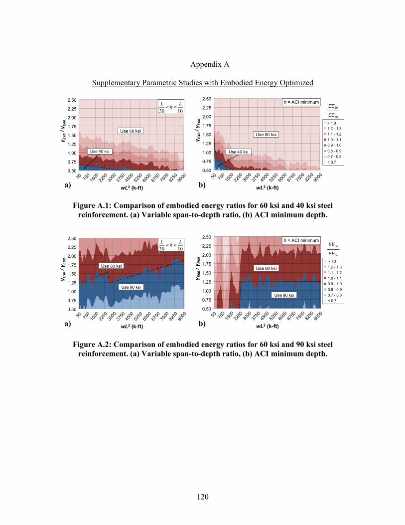
120
Appendix A
Supplementary Parametric Studies with Embodied Energy Optimized
Figure A.1: Comparison of embodied energy ratios for 60 ksi and 40 ksi steel reinforcement. (a) Variable span-to-depth ratio, (b) ACI minimum depth.
Figure A.2: Comparison of embodied energy ratios for 60 ksi and 90 ksi steel reinforcement. (a) Variable span-to-depth ratio, (b) ACI minimum depth.
0.50
0.75
1.00
1.25
1.50
1.75
2.00
2.25
2.50
50
800
1550
23
00
3050
38
00
4550
53
00
6050
68
00
7550
83
00
9050
γ E40
/ γ E
60
wL2 (k-ft)
1.30-1.40 1.20-1.30 1.10-1.20 1.00-1.10 0.90-1.00 0.80-0.90 0.70-0.80 0.60-0.70
Use 60 ksi
Use 40 ksi
50
5250
60
00
6750
75
00
3000
37
50
2250
1500
750
4500
9000
8250
L30
< h < L10
0.50
0.75
1.00
1.25
1.50
1.75
2.00
2.25
2.50
50
800
1550
23
00
3050
38
00
4550
53
00
6050
68
00
7550
83
00
9050
γ E40
/ γ E
60
wL2 (k-ft)
1.30-1.40 1.20-1.30 1.10-1.20 1.00-1.10 0.90-1.00 0.80-0.90 0.70-0.80 0.60-0.70
Use 60 ksi
Use 40 ksi
50
5250
60
00
6750
75
00
3000
37
50
2250
1500
750
4500
9000
8250
EE40
EE60
h = ACI minimum
0.9 - 1.0
> 1.3 1.2 - 1.3 1.1 - 1.2 1.0 - 1.1
0.8 - 0.9 0.7 - 0.8 < 0.7
0.50
0.75
1.00
1.25
1.50
1.75
2.00
2.25
2.50
50
800
1550
23
00
3050
38
00
4550
53
00
6050
68
00
7550
83
00
9050
γ E90
/ γ E
60
wL2 (k-ft)
1.30-1.40 1.20-1.30 1.10-1.20 1.00-1.10 0.90-1.00 0.80-0.90 0.70-0.80 0.60-0.70
Use 60 ksi
Use 90 ksi
50
5250
60
00
6750
75
00
3000
37
50
2250
1500
750
4500
9000
8250
L30
< h < L10
0.50
0.75
1.00
1.25
1.50
1.75
2.00
2.25
2.50
50
800
1550
23
00
3050
38
00
4550
53
00
6050
68
00
7550
83
00
9050
γ E90
/ γ E
60
wL2 (k-ft)
1.30-1.40 1.20-1.30 1.10-1.20 1.00-1.10 0.90-1.00 0.80-0.90 0.70-0.80 0.60-0.70
Use 60 ksi
Use 90 ksi
50
5250
60
00
6750
75
00
3000
37
50
2250
1500
750
4500
9000
8250
EE90
EE60
h = ACI minimum
0.9 - 1.0
> 1.3 1.2 - 1.3 1.1 - 1.2 1.0 - 1.1
0.8 - 0.9 0.7 - 0.8 < 0.7
a) b)
a) b)

121
Figure A.3: Comparison of embodied energy ratios for 60 ksi and 100 ksi steel reinforcement. (a) Variable span-to-depth ratio, (b) ACI minimum depth.
Figure A.4: Comparison of embodied energy ratios for 4,350 psi and 2,500 psi concrete. (a) Variable span-to-depth ratio, (b) ACI minimum depth.
Figure A.5: Comparison of embodied energy ratios for 4,350 psi and 8,000 psi concrete. (a) Variable span-to-depth ratio, (b) ACI minimum depth.
0.50
0.75
1.00
1.25
1.50
1.75
2.00
2.25
2.50
50
800
1550
23
00
3050
38
00
4550
53
00
6050
68
00
7550
83
00
9050
γ E10
0 / γ
E60
wL2 (k-ft)
1.30-1.40 1.20-1.30 1.10-1.20 1.00-1.10 0.90-1.00 0.80-0.90 0.70-0.80 0.60-0.70
Use 60 ksi
Use 100 ksi
50
5250
60
00
6750
75
00
3000
37
50
2250
1500
750
4500
9000
8250
L30
< h < L10 0.50
0.75
1.00
1.25
1.50
1.75
2.00
2.25
2.50
50
800
1550
23
00
3050
38
00
4550
53
00
6050
68
00
7550
83
00
9050
γ E10
0 / γ
E60
wL2 (k-ft)
1.30-1.40 1.20-1.30 1.10-1.20 1.00-1.10 0.90-1.00 0.80-0.90 0.70-0.80 0.60-0.70
Use 60 ksi
Use 100 ksi
50
5250
60
00
6750
75
00
3000
37
50
2250
1500
750
4500
9000
8250
EE100
EE60
h = ACI minimum
0.9 - 1.0
> 1.3 1.2 - 1.3 1.1 - 1.2 1.0 - 1.1
0.8 - 0.9 0.7 - 0.8 < 0.7
0.50
0.75
1.00
1.25
1.50
1.75
2.00
2.25
2.50
50
800
1550
23
00
3050
38
00
4550
53
00
6050
68
00
7550
83
00
9050
γ E25
00 / γ E
4350
wL2 (k-ft)
1.30-1.40 1.20-1.30 1.10-1.20 1.00-1.10 0.90-1.00 0.80-0.90 0.70-0.80 0.60-0.70
Use 4,350 psi
Use 2,500 psi
50
5250
60
00
6750
75
00
3000
37
50
2250
1500
750
4500
9000
8250
EE2500
EE4350
L30
< h < L10
0.9 - 1.0
> 1.3 1.2 - 1.3 1.1 - 1.2 1.0 - 1.1
0.8 - 0.9 0.7 - 0.8 < 0.7
0.50
0.75
1.00
1.25
1.50
1.75
2.00
2.25
2.50
50
800
1550
23
00
3050
38
00
4550
53
00
6050
68
00
7550
83
00
9050
γ E25
00 / γ E
4350
wL2 (k-ft)
1.30-1.40 1.20-1.30 1.10-1.20 1.00-1.10 0.90-1.00 0.80-0.90 0.70-0.80 0.60-0.70
Use 4,350 psi
Use 2,500 psi
50
5250
60
00
6750
75
00
3000
37
50
2250
1500
750
4500
9000
8250
EE2500
EE4350
h = ACI minimum
0.9 - 1.0
> 1.3 1.2 - 1.3 1.1 - 1.2 1.0 - 1.1
0.8 - 0.9 0.7 - 0.8 < 0.7
0.50
0.75
1.00
1.25
1.50
1.75
2.00
2.25
2.50
50
800
1550
23
00
3050
38
00
4550
53
00
6050
68
00
7550
83
00
9050
γ E80
00 / γ E
4350
wL2 (k-ft)
1.30-1.40 1.20-1.30 1.10-1.20 1.00-1.10 0.90-1.00 0.80-0.90 0.70-0.80 0.60-0.70
Use 4,350 psi
Use 8,000 psi
50
5250
60
00
6750
75
00
3000
37
50
2250
1500
750
4500
9000
8250
L30
< h < L10
0.50
0.75
1.00
1.25
1.50
1.75
2.00
2.25
2.50
50
800
1550
23
00
3050
38
00
4550
53
00
6050
68
00
7550
83
00
9050
γ E80
00 / γ E
4350
wL2 (k-ft)
1.30-1.40 1.20-1.30 1.10-1.20 1.00-1.10 0.90-1.00 0.80-0.90 0.70-0.80 0.60-0.70
Use 4,350 psi
Use 8,000 psi
50
5250
60
00
6750
75
00
3000
37
50
2250
1500
750
4500
9000
8250
EE8000
EE4350
h = ACI minimum
0.9 - 1.0
> 1.3 1.2 - 1.3 1.1 - 1.2 1.0 - 1.1
0.8 - 0.9 0.7 - 0.8 < 0.7
a) b)
a) b)
a) b)

122
Figure A.6: Aspect ratio for different grades of concrete when optimized for embodied energy. (a) One-half the baseline unit embodied energy of concrete, (b)
Two-and-a-half times the baseline unit embodied energy of concrete.
Figure A.7: Reinforcement ratio for different grades of concrete when optimized for embodied energy. (a) One-half the baseline unit embodied energy of concrete, (b)
Two-and-a-half times the baseline unit embodied energy of concrete.
Figure A.8: Recommended reinforcement ratio for different grades of concrete when optimized for embodied energy. (a) One-half the baseline unit embodied
energy of concrete, (b) Two-and-a-half times the baseline unit embodied energy of concrete.
0.0 0.1 0.2 0.3 0.4 0.5 0.6 0.7 0.8 0.9 1.0
0
1000
2000
3000
4000
5000
6000
7000
8000
9000
Asp
ect R
atio
[b / h]
wL2 (k-ft)
2,500 psi 4,350 psi 6,000 psi 8,000 psi 10,000 psi
Strength of Concrete
γEC = 0.65 MJ/kg
0.0 0.1 0.2 0.3 0.4 0.5 0.6 0.7 0.8 0.9 1.0
0
1000
2000
3000
4000
5000
6000
7000
8000
9000
Asp
ect R
atio
[b / h]
wL2 (k-ft)
2,500 psi 4,350 psi 6,000 psi 8,000 psi 10,000 psi
Strength of Concrete
γEC = 3.25 MJ/kg
0.000
0.005
0.010
0.015
0.020
0.025
0.030
0.035
0
1000
2000
3000
4000
5000
6000
7000
8000
9000
Rei
nfor
cem
ent R
atio
[ρ ]
wL2 (k-ft)
2,500 psi 4,350 psi 6,000 psi 8,000 psi 10,000 psi
Strength of Concrete
L30
< h < L10
0.000
0.005
0.010
0.015
0.020
0.025
0.030
0.035
0
1000
2000
3000
4000
5000
6000
7000
8000
9000
Rei
nfor
cem
ent R
atio
[ρ]
wL2 (k-ft)
2,500 psi 4,350 psi 6,000 psi 8,000 psi 10,000 psi
Strength of Concrete
γEC = 0.65 MJ/kg
0.000
0.005
0.010
0.015
0.020
0.025
0.030
0.035
0
1000
2000
3000
4000
5000
6000
7000
8000
9000
Rei
nfor
cem
ent R
atio
[ρ]
wL2 (k-ft)
2,500 psi 4,350 psi 6,000 psi 8,000 psi 10,000 psi
Strength of Concrete
γEC = 3.25 MJ/kg
0.000
0.005
0.010
0.015
0.020
0.025
0.030
0.035
0
1000
2000
3000
4000
5000
6000
7000
8000
9000
Rei
nfor
cem
ent R
atio
[ρ ]
wL2 (k-ft)
2,500 psi 4,350 psi 6,000 psi 8,000 psi 10,000 psi
Strength of Concrete
L30
< h < L10
0.0100 0.0135 0.0145 0.0152 0.0159
0.000
0.005
0.010
0.015
0.020
0.025
0.030
0.035
2,500
psi
4,350
psi
6,000
psi
8,000
psi
10,00
0 psi
Rec
omm
ende
d R
einf
orce
men
t Rat
io [ρ
]
Strength of Concrete
γEC = 0.65 MJ/kg
0.0104
0.0159 0.0189
0.0219 0.0257
0.000
0.005
0.010
0.015
0.020
0.025
0.030
0.035
2,500
psi
4,350
psi
6,000
psi
8,000
psi
10,00
0 psi
Rec
omm
ende
d R
einf
orce
men
t Rat
io [ρ
]
Strength of Concrete
γEC = 3.25 MJ/kg
a) b)
a) b)

123
Figure A.9: Span-to-depth ratio for different grades of concrete when optimized for embodied energy. (a) One-half the baseline unit embodied energy of concrete, (b)
Two-and-a-half times the baseline unit embodied energy of concrete.
Figure A.10: Comparison of embodied energy ratios for 145 pcf and 103 pcf concrete. (a) Variable-span-to depth ratio, (b) ACI minimum depth.
Figure A.11: Aspect ratio for different unit weights of concrete when optimized for embodied energy. (a) One-half the baseline unit embodied energy of concrete, (b)
Two-and-a-half times the baseline unit embodied energy of concrete.
8
10
12
14
16
18
20
22
24
26
0
1000
2000
3000
4000
5000
6000
7000
8000
9000
Spa
n-to
-Dep
th R
atio
[L /
h]
wL2 (k-ft)
2,500 psi 4,350 psi 6,000 psi 8,000 psi 10,000 psi
Strength of Concrete
ACI limit for required deflection calculations of simple span beams.
γEC = 0.65 MJ/kg
8
10
12
14
16
18
20
22
24
26
0
1000
2000
3000
4000
5000
6000
7000
8000
9000
Spa
n-to
-Dep
th R
atio
[L /
h]
wL2 (k-ft)
2,500 psi 4,350 psi 6,000 psi 8,000 psi 10,000 psi
Strength of Concrete
ACI limit for required deflection calculations of simple span beams.
γEC = 3.25 MJ/kg
0.000
0.005
0.010
0.015
0.020
0.025
0.030
0.035
0
1000
2000
3000
4000
5000
6000
7000
8000
9000
Rei
nfor
cem
ent R
atio
[ρ ]
wL2 (k-ft)
2,500 psi 4,350 psi 6,000 psi 8,000 psi 10,000 psi
Strength of Concrete
L30
< h < L10
0.50
0.75
1.00
1.25
1.50
1.75
2.00
2.25
2.50
50
800
1550
23
00
3050
38
00
4550
53
00
6050
68
00
7550
83
00
9050
γ E10
3 / γ
E145
wL2 (k-ft)
1.30-1.40 1.20-1.30 1.10-1.20 1.00-1.10 0.90-1.00 0.80-0.90 0.70-0.80 0.60-0.70
Use 145 pcf
Use 103 pcf
50
5250
60
00
6750
75
00
3000
37
50
2250
1500
750
4500
9000
8250
EE103
EE145
0.9 - 1.0
> 1.3 1.2 - 1.3 1.1 - 1.2 1.0 - 1.1
0.8 - 0.9 0.7 - 0.8 < 0.7
h = ACI minimum
0.0 0.1 0.2 0.3 0.4 0.5 0.6 0.7 0.8 0.9 1.0
0
1000
2000
3000
4000
5000
6000
7000
8000
9000
Asp
ect R
atio
[b / h]
wL2 (k-ft)
90 pcf 103 pcf 115 pcf 145 pcf
Unit Weight of Concrete
γEC = 0.65 MJ/kg
0.0 0.1 0.2 0.3 0.4 0.5 0.6 0.7 0.8 0.9 1.0
0
1000
2000
3000
4000
5000
6000
7000
8000
9000
Asp
ect R
atio
[b / h]
wL2 (k-ft)
90 pcf 103 pcf 115 pcf 145 pcf
Unit Weight of Concrete
γEC = 3.25 MJ/kg
0.0 0.1 0.2 0.3 0.4 0.5 0.6 0.7 0.8 0.9 1.0
0
1000
2000
3000
4000
5000
6000
7000
8000
9000
Asp
ect R
atio
[b / h]
wL2 (k-ft)
90 pcf 103 pcf 115 pcf 145 pcf
Unit Weight of Concrete
γEC = 0.65 MJ/kg
a) b)
a) b)
a) b)

124
Figure A.12: Reinforcement ratio for different unit weights of concrete when optimized for embodied energy. (a) One-half the baseline unit embodied energy of concrete, (b) Two-and-a-half times the baseline unit embodied energy of concrete.
Figure A.13: Recommended reinforcement ratio for different unit weights of concrete when optimized for embodied energy. (a) One-half the baseline unit
embodied energy of concrete, (b) Two-and-a-half times the baseline unit embodied energy of concrete.
Figure A.14: Span-to-depth ratio for different unit weights of concrete when optimized for embodied energy. (a) One-half the baseline unit embodied energy of concrete, (b) Two-and-a-half times the baseline unit embodied energy of concrete.
0.000
0.005
0.010
0.015
0.020
0.025
0.030
0.035
0
1000
2000
3000
4000
5000
6000
7000
8000
9000
Rei
nfor
cem
ent R
atio
[ρ]
wL2 (k-ft)
90 pcf 103 pcf 115 pcf 145 pcf
Unit Weight of Concrete
γEC = 0.65 MJ/kg
0.000
0.005
0.010
0.015
0.020
0.025
0.030
0.035
0
1000
2000
3000
4000
5000
6000
7000
8000
9000
Rei
nfor
cem
ent R
atio
[ρ]
wL2 (k-ft)
90 pcf 103 pcf 115 pcf 145 pcf
Unit Weight of Concrete
γEC = 3.25 MJ/kg
0.0 0.1 0.2 0.3 0.4 0.5 0.6 0.7 0.8 0.9 1.0
0
1000
2000
3000
4000
5000
6000
7000
8000
9000
Asp
ect R
atio
[b / h]
wL2 (k-ft)
90 pcf 103 pcf 115 pcf 145 pcf
Unit Weight of Concrete
γEC = 0.65 MJ/kg
0.0114 0.0119 0.0124 0.0135
0.000
0.005
0.010
0.015
0.020
0.025
0.030
0.035
90 p
cf
103 p
cf
115 p
cf
145 p
cf
Rec
omm
ende
d R
einf
orce
men
t Rat
io [ρ
]
Unit Weight of Concrete
γEC = 0.65 MJ/kg
0.0150 0.0151 0.0154 0.0159
0.000
0.005
0.010
0.015
0.020
0.025
0.030
0.035
90 p
cf
103 p
cf
115 p
cf
145 p
cf
Rec
omm
ende
d R
einf
orce
men
t Rat
io [ρ
]
Unit Weight of Concrete
γEC = 3.25 MJ/kg
8
10
12
14
16
18
20
22
24
26
0
1000
2000
3000
4000
5000
6000
7000
8000
9000
Spa
n-to
-Dep
th R
atio
[L /
h]
wL2 (k-ft)
90 pcf 103 pcf 115 pcf 145 pcf
Unit Weight of Concrete
ACI limit for required deflection calculations of simple span beams.
γEC = 0.65 MJ/kg
8
10
12
14
16
18
20
22
24
26
0
1000
2000
3000
4000
5000
6000
7000
8000
9000
Spa
n-to
-Dep
th R
atio
[L /
h]
wL2 (k-ft)
90 pcf 103 pcf 115 pcf 145 pcf
Unit Weight of Concrete
ACI limit for required deflection calculations of simple span beams.
γEC = 3.25 MJ/kg
0.0 0.1 0.2 0.3 0.4 0.5 0.6 0.7 0.8 0.9 1.0
0
1000
2000
3000
4000
5000
6000
7000
8000
9000
Asp
ect R
atio
[b / h]
wL2 (k-ft)
90 pcf 103 pcf 115 pcf 145 pcf
Unit Weight of Concrete
γEC = 0.65 MJ/kg
a) b)
a) b)
a) b)

125
Appendix B
Supplementary Parametric Studies with Cost Optimized
Figure B.1: Comparison of cost ratios for 60 ksi and 40 ksi steel reinforcement. (a) Variable span-to-depth ratio, (b) ACI minimum depth.
Figure B.2: Comparison of cost ratios for 4,350 psi and 2,500 psi concrete. (a) Variable span-to-depth ratio, (b) ACI minimum depth.
0.50
0.75
1.00
1.25
1.50
1.75
2.00
2.25
2.50
50
800
1550
23
00
3050
38
00
4550
53
00
6050
68
00
7550
83
00
9050
γ $40
/ γ $
60
wL2 (k-ft)
1.30-1.40 1.20-1.30 1.10-1.20 1.00-1.10 0.90-1.00 0.80-0.90 0.70-0.80 0.60-0.70
Use 60 ksi
50
5250
60
00
6750
75
00
3000
37
50
2250
1500
750
4500
9000
8250
C40
C60
0.9 - 1.0
> 1.3 1.2 - 1.3 1.1 - 1.2 1.0 - 1.1
0.8 - 0.9 0.7 - 0.8 < 0.7
Use 40 ksi
L30
< h < L10
0.50
0.75
1.00
1.25
1.50
1.75
2.00
2.25
2.50
50
800
1550
23
00
3050
38
00
4550
53
00
6050
68
00
7550
83
00
9050
γ $40
/ γ $
60
wL2 (k-ft)
1.30-1.40 1.20-1.30 1.10-1.20 1.00-1.10 0.90-1.00 0.80-0.90 0.70-0.80 0.60-0.70
Use 60 ksi
50
5250
60
00
6750
75
00
3000
37
50
2250
1500
750
4500
9000
8250
C40
C60
0.9 - 1.0
> 1.3 1.2 - 1.3 1.1 - 1.2 1.0 - 1.1
0.8 - 0.9 0.7 - 0.8 < 0.7
Use 40 ksi
h = ACI minimum
0.50
0.75
1.00
1.25
1.50
1.75
2.00
2.25
2.50
50
800
1550
23
00
3050
38
00
4550
53
00
6050
68
00
7550
83
00
9050
γ $25
00 / γ $
4350
wL2 (k-ft)
1.30-1.40 1.20-1.30 1.10-1.20 1.00-1.10 0.90-1.00 0.80-0.90 0.70-0.80 0.60-0.70
Use 4,350 psi
50
5250
60
00
6750
75
00
3000
37
50
2250
1500
750
4500
9000
8250
C2500
C4350
0.9 - 1.0
> 1.3 1.2 - 1.3 1.1 - 1.2 1.0 - 1.1
0.8 - 0.9 0.7 - 0.8 < 0.7
Use 2,500 psi
L30
< h < L10
0.50
0.75
1.00
1.25
1.50
1.75
2.00
2.25
2.50
50
800
1550
23
00
3050
38
00
4550
53
00
6050
68
00
7550
83
00
9050
γ $25
00 / γ $
4350
wL2 (k-ft)
1.30-1.40 1.20-1.30 1.10-1.20 1.00-1.10 0.90-1.00 0.80-0.90 0.70-0.80 0.60-0.70
Use 4,350 psi
50
5250
60
00
6750
75
00
3000
37
50
2250
1500
750
4500
9000
8250
C2500
C4350
0.9 - 1.0
> 1.3 1.2 - 1.3 1.1 - 1.2 1.0 - 1.1
0.8 - 0.9 0.7 - 0.8 < 0.7
Use 2,500 psi
h = ACI minimum
a) b)
a) b)

126
Figure B.3: Comparison of cost ratios for 145 pcf and 115 pcf concrete. (a) Variable span-to-depth ratio, (b) ACI minimum depth.
0.50
0.75
1.00
1.25
1.50
1.75
2.00
2.25
2.50
50
800
1550
23
00
3050
38
00
4550
53
00
6050
68
00
7550
83
00
9050
γ $11
5 / γ
$145
wL2 (k-ft)
1.30-1.40 1.20-1.30 1.10-1.20 1.00-1.10 0.90-1.00 0.80-0.90 0.70-0.80 0.60-0.70
Use 145 pcf 50
5250
60
00
6750
75
00
3000
37
50
2250
1500
750
4500
9000
8250
C115
C145
0.9 - 1.0
> 1.3 1.2 - 1.3 1.1 - 1.2 1.0 - 1.1
0.8 - 0.9 0.7 - 0.8 < 0.7
Use 115 pcf
L30
< h < L10
0.50
0.75
1.00
1.25
1.50
1.75
2.00
2.25
2.50
50
800
1550
23
00
3050
38
00
4550
53
00
6050
68
00
7550
83
00
9050
γ $11
5 / γ
$145
wL2 (k-ft)
1.30-1.40 1.20-1.30 1.10-1.20 1.00-1.10 0.90-1.00 0.80-0.90 0.70-0.80 0.60-0.70
Use 145 pcf
50
5250
60
00
6750
75
00
3000
37
50
2250
1500
750
4500
9000
8250
C115
C145
0.9 - 1.0
> 1.3 1.2 - 1.3 1.1 - 1.2 1.0 - 1.1
0.8 - 0.9 0.7 - 0.8 < 0.7 Use 115 pcf
h = ACI minimum

127
Appendix C
Extended Bibliography
Beams
Adamu, A., Karihaloo, B. L., & Rozvany, G. I. N. (1994). Minimum cost design of reinforced concrete beams using continuum-type optimality criteria.
Alqedra, M., Arafa, M., & Ismail, M. (2011). Optimum cost of prestressed and reinforced concrete beams using genetic algorithms.
Alreshaid, K., Mahdi, I. M., & Soliman, E. (2004). Cost optimization of reinforced concrete elements.
Al-Salloum, Y. A., & Siddiqi, G. H. (1994). Cost-optimum design of reinforced concrete (RC) beams.
Balaguru, P. (1980). Optimum design of singly reinforced rectangular sections. Balaguru, P. N. (1980). Cost optimum design of doubly reinforced concrete beams. Balaguru, P. N. (1980). Optimum design of T beam sections. Balaguru, P., & Courel, M. (1984). Cost optimum design of reinforced concrete slabs and
beams using programmable calculators.
Chakrabarty, B. K. (1992). Model for optimal design of reinforced concrete beam. Chakrabarty, B. K. (1992). Models for optimal design of reinforced concrete beams. Chou, T. (1977). Optimum reinforced concrete T-beam sections. Chung, T. T., & Sun, T. C. (1994). Weight optimization for flexural reinforced concrete
beams with static nonlinear response.
Coello, C. C., Hernandez, F. S., & Farrera F. A. (1997). Optimal design of reinforced concrete beams using genetic algorithms.
Coello Coello, C. A., Christiansen, A. D., & Santos Hernandez F. (1997). A simple genetic algorithm for the design of reinforced concrete beams.
Colin, M. Z., & MacRae, A. J. (1984). Optimization of structural concrete beams.

128
Erbatur, H. F., & Samman, M. M. (1987). Optimum design of reinforced concrete beams. Ezeldin, A. S., & Hsu, C. T. T. (1992). Optimization of reinforced fibrous concrete
beams.
Friel, L. L. (1974). Optimum singly reinforced concrete sections. Govindaraj, V., & Ramasamy, J. V. (2005). Optimum detailed design of reinforced concrete continuous beams using genetic algorithms. Kanagasundaram, S., & Karihaloo, B. L. (1990). Minimum cost design of reinforced
concrete structures.
Kanagasundaram, S., & Karihaloo, B. L. (1991). Minimum-cost reinforced concrete beams and columns.
Kirsch, U. (1983). Multilevel optimal design of reinforced concrete structures. Koumousis, V. K., & Arsenis, S. J. (1998). Genetic algorithms in optimal detailed design
of reinforced concrete members.
Lakshmanan, N., & Parameswaran, V. S. (1985). Minimum weight design of reinforced concrete sections for flexure.
Leps, M., & Sejnoha, (2003). M. New approach to optimization of reinforced concrete beams. Prakash, A., Agarwala, S. K., & Singh, K.K. (1988). Optimum design of reinforced
concrete sections.
Samman, M. M., & Erbatur, H. F. (1995). Steel ratios for cost optimum reinforced concrete beams.
Yeo, D. H., & Gabbai, R. D. (2011). Sustainable design of reinforced concrete structures through embodied energy optimization.
Columns
Rafiq, M., Packman, I., Easterbrook, D., & Denham, S. (2006). Visualizing search and solution spaces in the optimum design of biaxial columns. Rafiq, M.Y., & Southcombe, C. (1998). Genetic algorithms in optimal design and
detailing of reinforced concrete biaxial columns supported by a declarative approach for capacity checking.

129
Frames
Balling, R. J., & Yao, X. (1997). Optimization of reinforced concrete frames. Booz, W., Legewie, G., Thierauf, G., & Statik, F. B. (1984). Optimization of reinforced
concrete structures according to German design regulations.
Camp, C. V., & Huq, F. (2013). CO2 and cost optimization of reinforced concrete frames using a big bang-big crunch algorithm.
Camp, C.V., Pezeshk, S., & Hansson, H. (2003). Flexural design reinforced concrete frames using a genetic algorithm. Choi, C. K., & Kwak, H. G. (1990). Optimum RC member design with predetermined
discrete sections.
Gencturk, B., & Elnashai, A. S. (2011). Optimal whole-life-cycle seismic design of concrete frames.
Hoit, M., Soeiro, A., & Fagundo, F. (1991). Probabilistic design and optimization of reinforced concrete frames.
Huanchun, S., & Zheng, C. (1985). Two-level optimum design of reinforced concrete frames with integer variables.
Krishnamoorthy, C. S., & Mosi, D. R. (1981). Optimal design of reinforced concrete frames based on inelastic analysis.
Krishnamoorthy, C. S., & Munro, J. (1973). Linear program for optimal design of reinforced concrete frames.
Krishnamoorthy, C. S., Munro, J., & Yu, C. W. (1972). Optimal design of reinforced concrete frames.
Krishnamoorthy, C. S., & Rajeev, S. (1989). Computer-aided optimal design of
reinforced concrete frames.
Kwak, H.G., & Kim, J. (2008). Optimum design of reinforced concrete plane frames based on predetermined section database. Kwak, H.G., & Kim, J. (2009). An integrated genetic algorithm complemented with direct search for optimum design of RC frames.

130
Lee, C., & Ahn, J. (2003). Flexural design reinforced concrete frames by genetic algorithm. Moharrami, H., & Grierson, D. E. (1993). Computer-automated design of reinforced
concrete frameworks.
Paya, I., Yepes, V., Gonzalez-Vidosa, F., & Hospitaler, A. (2008). Multiobjective optimization of concrete frames by simulated annealing. Paya-Zaforteza, I., Yepes, V., Clemente, J., & Gonzalez-Vidosa, F. (2006). Heuristic optimization of reinforced concrete building frames. Paya-Zaforteza, I., Yepes, V., Hospitaler, A., & Gonzalez-Vidosa, F. (2009). CO2-
efficient design of reinforced concrete building frames.
Paya-Zaforteza, I., Yepes, V., Hospitaler, A., & Gonzalez-Vidosa, F. (2009). CO2 optimization of reinforced concrete frames by simulated annealing. Rajeev, S., & Krisnamoorthy, C. S. (1998). Genetic algorithm-based methodology for design optimization of reinforced concrete frames. Rozvany, G. I. N., & Cohn, M. Z. (1970). Lower-bound optimal design of concrete
structures.
Val, D., Bljuger, F., & Yankelevsky, D. (1996). Optimization problem solution in reliability analysis of reinforced concrete structures.
Yeo, D. H., & Potra, F. (2013). Sustainable design of reinforced concrete structures through CO2 emission optimization.
Retaining Structures
Ahmadi-Nedushan, B., & Varaee, H. (2009). Optimal design of reinforced concrete
retaining walls using a swarm intelligence technique.
Alcala, J., Carrera, M., Gonzalez, F., & Yepes, V. (2005). A simulated annealing approach to the economic optimization of reinforced concrete cantilever retaining walls.
Alshawi, F. A. N., Mohammed, A. I., & Farid, B. J. (1988). Optimum design of tied-back retaining walls.
Babu, G. L. S., & Basha, B. M. (2008). Optimum design of cantilever retaining walls using target reliability approach.

131
Basudhar, P. K., Vashistha, A., Deb, K., & Dey, A. (2008). Cost optimization of reinforced earth walls.
Bhatti, M. A. (2006). Retaining wall design optimization with MS Excel solver. Camp, C.V., & Akin A. (2012). Design of retaining walls using big bang-big crunch
optimization.
Ceranic, B., Fryer, C., & Baines, R. W. (2001). An application of simulated annealing to the optimum design of reinforced concrete retaining structure.
Chau, K. W., & Albermani, F. (2003). Knowledge-based system on optimum design of liquid retaining structures with genetic algorithms.
Fang, H. Y., Atsuta, T., & Chen, W. F. (1980). Optimum design of retaining walls on sloping hillside.
Kaveh, A., & Abadi, A. S. M. (2010). Harmony search based algorithm for the optimum cost design of reinforced concrete cantilever retaining walls.
Keskar, A. V., & Adidam, S. R. (1989). Minimum cost design of a cantilever retaining wall.
Khajehzadeh, M., Taha, M. R., El-Shafie, A., & Eslami, M. (2011). Modified particle swarm optimization for optimum design of spread footing and retaining wall.
Rhomberg, E. J., & Street, W. M. (1981). Optimal design of retaining walls. Saribaş, A., & Erbatur, F. (1996). Optimization and sensitivity of retaining structures. Villalba, P., Alcala, J., Yepes, V., & Gonzalez-Vidosa, F. (2010). CO2 optimization of
reinforced concrete cantilever retaining walls.
Yepes, V. (2006). Heuristic optimization applied to the economic design of reinforced concrete earth retaining walls.
Yepes, V., Alcala, J., Perea, C., & Gonzalez-Vidosa, F. (2008). A parametric study of optimum earth retaining walls by simulated annealing.
Yepes, V., Gonzalez-Vidosa, F., Alcala, J., & Villalba, P. (2012). CO2-optimization design of reinforced concrete retaining walls based on a VNS-threshold acceptance strategy.

132
Bridge Components
Jenkins, D., Portella, J., & Baweja, D. (2011). Optimising precast bridge girders for sustainability with the use of high performance concrete.
Martinez, F. J., Gonzalez-Vidosa, F., Hospitaler, A., & Yepes, V. (2010). Heuristic optimization of RC bridge piers with rectangular hollow sections.
Martinez, F., Yepes, V., Hospitaler, A., & Gonzalez-Vidosa, F. (2007). Ant colony optimization of reinforced concrete bridge piers of rectangular hollow section. Perea, C., Alcala, J., Yepes, V., Gonzalez-Vidosa, F., & Hospitaler, A. (2008). Design of
reinforced concrete bridge frames by heuristic optimization.
Perea, C., Baitsch, M., Gonzalez-Vidosa, F., & Hartmann, D. (2007). Optimization of reinforced concrete frame bridges by parallel genetic and memetic algorithms.
Other
Camp, C. V., & Assadollahi, A. (2013). CO2 and cost optimization of reinforced concrete footings using a hybrid big bang-big crunch algorithm.
Carbonell, A., Gonzalez-Vidosa, F., & Yepes, V. (2011). Design of reinforced concrete road vaults by heuristic optimization. Fadaee, M. J., & Grierson, D. E. (1996). Design optimization of 3D reinforced concrete
structures.
Gonzalez-Vidosa, F., Yepes, V., Alcala, J., Carrera, M., & Perea, C. (2005). Simulated annealing optimization of walls, portal and box reinforced concrete road structures. Perea, C., Paya, I., Yepes, V., & Gonzalez, F. (2006). Heuristic optimization of reinforced concrete road bridge frames. Sahab, M. G., Ashour, A.F., & Toropov, V. V. (2005). A hybrid genetic algorithm for
reinforced concrete flat slab buildings.
Sahab, M.G., Ashour, A.F., & Toporov, V.V. (2005). Cost optimization of reinforced concrete flat slab buildings.

133
REFERENCES
ACI Committee 318. (2011). Building code requirements for structural concrete. Farmington Hills, MI: American Concrete Institute.
ACI Committee 363. (1992). State-of-the-art report on high-strength concrete. ACI 363R- 92. Detroit, MI: American Concrete Institute. Alcorn, A. (2003). Embodied energy and co2 coefficients for nz building materials. Informally published manuscript, Centre for Building Performance Research, Victoria University of Wellington, Wellington, New Zealand. Retrieved from http://www.victoria.ac.nz/cbpr/documents/pdfs/ee-co2_report_2003.pdf Ali, L., & Fiaz, A. (2009). Use of fly ash alongwith blast furnace slag as partial
replacement of fine aggregate and mineral filler in asphalt mix, at high temperature. Geohunan International Conference. Retrieved from http://ascelibrary.org/doi/pdf/10.1061/41045%28352%2918
Alqedra, M., Arafa, M., & Ismail, M. (2011). Optimum cost of prestressed and reinforced concrete beams using genetic algorithms. Journal of Artificial Intelligence, 4(1), 76-88. Retrieved from http://scialert.net/qredirect.php?doi=jai.2011.76.88&linkid=pdf
Alreshaid, K., Mahdi, I. M., & Soliman, E. (2004). Cost optimization of reinforced concrete elements. Asian Journal of Civil Engineering, 5, 161-174. http://citeseerx.ist.psu.edu/viewdoc/download?doi=10.1.1.113.3758&rep=rep1&type=pdf
ASCE 7. (2010). Minimum design loads for buildings and other structures. New York, NY: American Society of Civil Engineers.
ASTM International A615. (2012). Standard Specification for Deformed and Plain Carbon-Steel Bars for Concrete Reinforcement. West Conshohocken, PA: American Society for Testing and Materials.
Camp, C., & Akin, A. (2012). Design of retaining walls using big bang-big crunch optimization. Journal of Structural Engineering, 138(3), 438-448. http://ascelibrary.org/doi/abs/10.1061/(ASCE)ST.1943-541X.0000461
Camp, C. V., & Assadollahi, A. (2013). CO2 and cost optimization of reinforced concrete
footings using a hybrid big bang-big crunch algorithm. Structural and Multidisciplinary Optimization, 48(2), 411-426. http://link.springer.com/article/10.1007/s00158-013-0897-6

134
Camp, C., & Huq, F. (2013). CO2 and cost optimization of reinforced concrete frames using a big bang-big crunch algorithm. Engineering Structures, 48, 363-372.
Camp, C. V., Pezeshk, S., & Hansson, H. (2003). Flexural design of reinforced concrete frames using a genetic algorithm. Journal of Structural Engineering, 129(1), 105– 115. Retrieved from http://ascelibrary.org/doi/abs/10.1061/(ASCE)0733-9445(2003)129:1(105)
Chou, T. (1977). Optimum reinforced concrete t-beam sections. Journal of the Structural Division, 103(ST8), 1605-1617. Retrieved from http://trid.trb.org/view.aspx?id=59696
Coello Coello, C. A., Christiansen, A. D., & Santos Hernandez, F. (1997). A simple genetic algorithm for the design of reinforced concrete beams. Engineering with Computers, 13(4), 185-196. Retrieved from http://link.springer.com/article/10.1007/BF01200046
Concrete Joint Sustainability Initiative. (2009). Reinforcement. Retrieved from website: http://www.sustainableconcrete.org/?q=node/144
Erol, O. K., & Eksin, I. (2006). A new optimization method: Big bang–big crunch. Advances in Engineering Software, 37(2), 106–111. Retrieved from http://www.sciencedirect.com/science/article/pii/S0965997805000827
Govindaraj, V., & Ramasamy, J. V. (2005). Optimum detailed design of reinforced concrete continuous beams using genetic algorithms. Computers & Structures, 84(1-2), 34-48. http://www.sciencedirect.com/science/article/pii/S004579490500310X
Guerra, A., Newman, A. M., & Leyffer, S. (2011). Concrete structure design using mixed-integer nonlinear programming with complementarity constraints. SIAM Journal on Optimization, 21(3), 833 - 863. Retrieved from http://inside.mines.edu/~aguerra/RCpaper_SIAMPUB.pdf
Hammond, G., & Jones, C. (2008). Inventory of carbon & energy (ice). Informally published manuscript, Department of Mechanical Engineering, University of Bath, Retrieved from http://perigordvacance.typepad.com/files/inventoryofcarbonandenergy.pdf
Holm, T. A., & Ries, J. P. (2006). Lightweight concrete and aggregates. ASTM: Significance of tests and properties of concrete and concrete-making materials. West Conshohocken, PA: American Society for Testing and Materials.

135
Johnson, J. B. (2010). Bond strength of corrosion resistant steel reinforcement in concrete. Informally published manuscript. Civil Engineering, Virginia Tech, Blacksburg, VA. Retrieved from http://www.moen.cee.vt.edu/postedfiles/Johnson_report_final.pdf
Kohonen, J. (1999). A brief comparison of simulated annealing and genetic algorithm approaches. Unpublished manuscript, Department of Computer Science, University of Helsinki, Retrieved from http://www.cs.helsinki.fi/u/kohonen/papers/gasa.html
Leps, M., & Sejnoha, M. (2003). New approach to optimization of reinforced concrete beams. Computers & Structures, 81(18-19), 1957–1966. Retrieved from http://www.sciencedirect.com/science/article/pii/S0045794903002153
Leroy, L. F. (1974). Optimum singly reinforced concrete sections. Journal Proceedings, 71(11), 556-558. Retrieved from http://www.concrete.org/PUBS/JOURNALS/OLJDetails.asp?Home=JP&ID=708 7
Mathworks. (2012). MATLAB [computer software]. Natick, Massachusetts: The MathWorks Inc.
Mathworks, (2013). What is direct search? Natick, Massachusetts: The MathWorks Inc. Retrieved from website: http://www.mathworks.com/help/gads/what-is-direct-search.html
Martinez, F., Yepes, V., Hospitaler, A., & Gonzalez-Vidosa, F. (2007). Ant colony optimization of reinforced concrete bridge piers of rectangular hollow section. Computational & Technology Resources, Retrieved from http://www.ctresources.info/ccp/paper.html?id=4661
Mehta, P., & Monteiro, P. (2006). Concrete: Microstructure, properties, and materials. (3rd ed.). New York, NY: The McGraw-Hill Companies, Inc.
Microsoft. (2011). Microsoft Excel [computer software]. Redmond, Washington: Microsoft.
MMFX Technologies Corporation. (2012). Material properties and design considerations. Irvine, CA: MMFX Technologies Corporation.
National Ready Mixed Concrete Association. (2003). CIP 36: Structural lightweight concrete. Retrieved from website: http://www.nrmca.org/aboutconcrete/cips/36p.pdf

136
Paya, I., Yepes, V., Gonzalez-Vidosa, F., & Hospitaler, A. (2008). Multiobjective optimization of concrete frames by simulated annealing. Computer-Aided Civil and Infrastructure Engineering, 23(8), 596–610. Retrieved from http://onlinelibrary.wiley.com/doi/10.1111/j.1467-8667.2008.00561.x/full
Paya-Zaforteza, I., Yepes, V., Hospitaler, A., & Gonzalez-Vidosa, F. (2009). Co2- optimization of reinforced concrete frames by simulated annealing. Engineering Structures, 31(7), 1501–1508. Retrieved from http://www.sciencedirect.com/science/article/pii/S0141029609000996
Rajeev, S., & Krishnamoorthy, C. S. (1998). Genetic algorithm-based methodology for design optimization of reinforced concrete frames. Computer-aided Civil and Infrastructure Engineering, 13(1), 63-74. Retrieved from http://onlinelibrary.wiley.com.libproxy.clemson.edu/doi/10.1111/0885- 9507.00086/abstract;jsessionid=7170B64D16BD5EE937553EC4B5E4B390.f03t 01
Rodriguez, J. [Web log message]. Retrieved from http://construction.about.com/od/Specifications/tp/Concrete-Admixtures-List-Of-Common-Used-Concrete-Admixtures.htm
Rozvany, G. I. N. (1970). Lower-bound optimal design of concrete structures. Journal of the Engineering Mechanics Division, 96(6), 1013-1030. Retrieved from http://cedb.asce.org/cgi/WWWdisplay.cgi?16674
Sahab, M. G., Ashour, A. F., & Toropov, V. V. (2005). Cost optimisation of reinforced concrete flat slab buildings. Engineering Structures, 27(3), 313-322. Retrieved from http://www.sciencedirect.com/science/article/pii/S014102960400330X
Samman, M. M., & Erbatur, H. F. (1995). Steel ratios for cost optimum reinforced concrete beams. Building and Environment, 30(4), 545–551. Retrieved from http://www.sciencedirect.com/science/article/pii/036013239500017Z
Suppapitnarm, A., Seffen, K. A., Parks, G. T., & Clarkson, P. J. (2000). A simulated annealing algorithm for multiobjective optimization. Engineering Optimization, 33(1), 59-85. Retrieved from http://www.tandfonline.com/doi/pdf/10.1080/03052150008940911
Table of embodied energy coefficients. (2007). Unpublished raw data. Centre for Building Performance Research, Victoria University of Wellington, Wellington, New Zealand. Retrieved from http://www.victoria.ac.nz/cbpr/documents/pdfs/ee-coefficients.pdf

137
The Concrete Countertop Institute. (2006). The role of aggregate in concrete countertop mixes. Retrieved from website: http://www.concretecountertopinstitute.com/library.item.41/the-role-of-aggregate-in-concrete-countertop-mixes.html
Waier, P. (Ed.). (2012). RSMeans building construction cost data (71st ed.). Norwell, MA: RS Means.
Worrell, E., Price, L., Martin, N., Hendriks, C., & Meida, L. O. Annual Review of Energy and the Environment. (2001). Carbon dioxide emissions from the global cement industry. Retrieved from Annual Reviews website: http://www.annualreviews.org/doi/pdf/10.1146/annurev.energy.26.1.303
Yeo, D., & Gabbai, R. D. (2011). Sustainable design of reinforced concrete through embodied energy optimization. Energy and Buildings, 43(8), 2028-2033. http://www.sciencedirect.com/science/article/pii/S0378778811001678#
Yeo, D., & Potra, F. A. (2013). Sustainable design of reinforced concrete structures through CO2 emission optimization. Journal of Structural Engineering. http://ascelibrary.org/doi/pdf/10.1061/%28ASCE%29ST.1943-541X.0000888