Embed Size (px)
Citation preview
COST ESTIMATION OF FRP WRAPPING FOR BRIDGE REHABILITATION USING
REGRESSION ANALYSIS
Srikanth Manukonda
Problem Report submitted to the
College of Engineering and Mineral Resources
at West Virginia University
in partial fulfillment of the requirements
for the degree of
Master of Science
in
Industrial Engineering
Robert C. Creese, Ph.D., Chair
Hota V. Gangarao, Ph.D.
Majid Jaraiedi, Ph.D.
Department of Industrial and Management Systems Engineering
Morgantown, West Virginia
2011
Keywords: Fiber Reinforced Polymer (FRP), FRP Wrapping, Cost, Regression
ii
ABSTRACT
Cost Estimation of FRP Wrapping for Bridge Rehabilitation Using Regression Analysis
Srikanth Manukonda
Fiber Reinforced Polymer (FRP) materials are replacing common construction materials
including steel, in reconstruction applications. Because of their structural advantages, such as,
durability, high strength to weight ratios, and high impact strength. FRP wraps are becoming
more reliable. In spite of having many bridge rehabilitation techniques, FRP wrapping is
preferred because of its ease of installation and durability.
FRP materials were introduced recently into civil infrastructure, while in aviation,
defense, and marine industries, FRP materials have been used for a longer time. The FRP
wrapping technique has been used to do many different kinds of bridge rehabilitations in the
United States. One type of bridge rehabilitation is the application of FRP wraps to repair and
strengthen different bridge elements, such as columns, beams, girders, and piles.
Regression analysis was done to estimate the contract values of FRP wrapping for bridge
rehabilitation projects using data from different projects. The data was provided by FYFE Co.
LLC and the Constructed Facilities Center at West Virginia University (CFC-WVU). The
variables studied were: the number of layers, the number of elements, the repair area, the type of
material, the type of application, and the product of layers and area. All the significant variables
were considered in building the regression equations. Two regression equations were built
separately, one for each columns and girders. Another equation was built for all contract values
with all element types. The variables ‘element type’, ‘number of layers’, ‘area’, ‘number of
elements’ and ‘number of layers × area’ were obtained as significant variables. Number of
layers was the most significant variable and it is present in all regression equations.
iii
TABLE OF CONTENTS
ABSTRACT ................................................................................................................................................. ii
LIST OF FIGURES .................................................................................................................................... v
LIST OF TABLES ..................................................................................................................................... vi
LIST OF ACRONYMS ........................................................................................................................... viii
CHAPTER 1 ................................................................................................................................................ 1
INTRODUCTION ....................................................................................................................................... 1
1.1 Introduction ......................................................................................................................................... 1
1.1.1 Rehabilitation Methods ............................................................................................................... 1
1.2 Objectives ........................................................................................................................................... 4
1.3 Limitations .......................................................................................................................................... 5
1.4 Organization of the Report .................................................................................................................. 5
CHAPTER 2 ................................................................................................................................................ 6
BACKGROUND AND LITERATURE REVIEW ................................................................................... 6
2.1 Background ......................................................................................................................................... 6
2.1.1 Fiber Reinforced Polymers (FRP) ................................................................................................ 6
2.1.1.1 Fibers ..................................................................................................................................... 6
2.1.1.2 Matrices ................................................................................................................................. 9
2.1.2 FRP Manufacturing Methods ..................................................................................................... 10
2.1.2.1 Compression Molding ......................................................................................................... 10
2.1.2.2 Resin Transfer Molding (RTM) .......................................................................................... 10
2.1.2.3 Pultrusion ............................................................................................................................ 10
2.1.2.4 Hand Lay-up ....................................................................................................................... 11
2.1.3 FRP Wrap Manufacturing .......................................................................................................... 11
2.1.4 FRP Wraps – A Historical View ................................................................................................ 12
2.2 Literature review ............................................................................................................................... 13
2.2.1 Economic Aspects of FRP Wraps .............................................................................................. 16
2.2.2 Review of Previous Models ....................................................................................................... 17
CHAPTER 3 .............................................................................................................................................. 19
METHODOLOGY ................................................................................................................................... 19
3.1 FRP Application Procedure .............................................................................................................. 19
3.1.1 Surface Preparation .................................................................................................................... 20
iv
3.1.2 Installation of FRP Wrap ........................................................................................................... 20
3.1.3 Non-Destructive Testing (NDT) ................................................................................................ 20
3.2 Data ................................................................................................................................................... 21
3.2 Variables ........................................................................................................................................... 27
3.2.1 Classification of Variables (factors)........................................................................................... 28
3.2.2 Explanation of Variables: ........................................................................................................... 29
3.3 The Regression Equation .................................................................................................................. 32
CHAPTER 4 .............................................................................................................................................. 34
RESULTS AND DISCUSSION ............................................................................................................... 34
4.1 Regression Using All Variables ........................................................................................................ 34
4.2 Regression only with Element Type ‘Column’ ................................................................................. 37
4.3 Regression on values with Element Type ‘Girders’ ......................................................................... 40
4.4 Regression on values with Element Type ‘Piles’ .............................................................................. 42
4.5 Summary of results ........................................................................................................................... 44
CHAPTER 5 .............................................................................................................................................. 45
CONCLUSIONS AND RECOMMENDATIONS .................................................................................. 45
5.1 Conclusions ....................................................................................................................................... 45
5.2 Recommendations ............................................................................................................................. 47
APPENDIX A ............................................................................................................................................ 49
DATA SHEET ............................................................................................................................................ 49
REFERENCES .......................................................................................................................................... 51
v
LIST OF FIGURES
Figure 1-1: A column under repair using concrete jacketing (www.payon-co.com) ..................... 2
Figure 1-2: A column repaired using steel jacketing (www.thecontructor.org) ............................. 2
Figure 1-3: A beam repaired using steel plate bonding (www.chemcosystems.com) .................... 3
Figure 1-4: An FRP wrap being applied on a wooden pile (P.V.Vijay, 2011) ............................... 4
Figure 2-1: Flexural and shear strengthening of beams ................................................................ 13
Figure 2-2: Example of contact critical application (column wrapping) ...................................... 13
Figure 2-3: Distribution of material costs ..................................................................................... 16
Figure 2-4: Distribution of labor ................................................................................................... 16
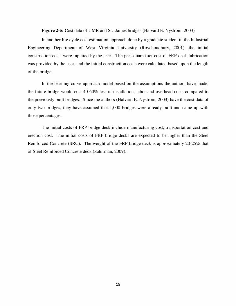
Figure 2-5: Cost data of UMR and St. James bridges (Halvard E. Nystrom, 2003) .................... 18
Figure 4-1: Stepwise regression analysis report on columns and girders ..................................... 34
Figure 4-2: Stepwise regression analysis report on columns ........................................................ 38
Figure 4-3: 95% confidence interval for contract values for columns .......................................... 40
Figure 4-4: Stepwise regression analysis report on girders .......................................................... 41
vi
LIST OF TABLES
Table 2-1: Material properties of glass fibers (David Hartman, 1996) ......................................................... 7
Table 2-2: Physical properties of glass fibers (David Hartman, 1996) ......................................................... 8
Table 2-3: Mechanical properties of carbon fibers (corecomposites.com, 2005) ......................................... 9
Table 2-4: Material properties of thermosetting and thermoplastic polymers (Clyne, 1996) ..................... 10
Table 3-1: Total contract values of different FRP wrapping projects undertaken by FYFE Co.LLC
Company ..................................................................................................................................................... 21
Table 3-2: Data description of different FRP wrapping projects undertaken by CFC at WVU ................. 21
Table 3-3: Material and labor costs of CFC-WVU projects (P.V.Vijay, 2011) ......................................... 22
Table 3-4: Individual project costs of CFC-WVU FRP Pile wrapping projects ......................................... 22
Table 3-5: Total contract values of all projects undertaken by both FYFE Co.LLC and CFC-WVU ....... 23
Table 3-6: Estimated Man hours spent on labor transportation for the projects done by FYFE Co.LLC .. 24
Table 3-7: Transportation costs for the projects undertaken by FYFE Co.LLC ......................................... 25
Table 3-8: Transportation costs for the projects undertaken by CFC-WVU .............................................. 25
Table 3-9: Contract values adjusted to 2011 inflation rates ........................................................................ 27
Table 3-10: List of predictor variables ........................................................................................................ 29
Table 3-11: Classification of application types ........................................................................................... 30
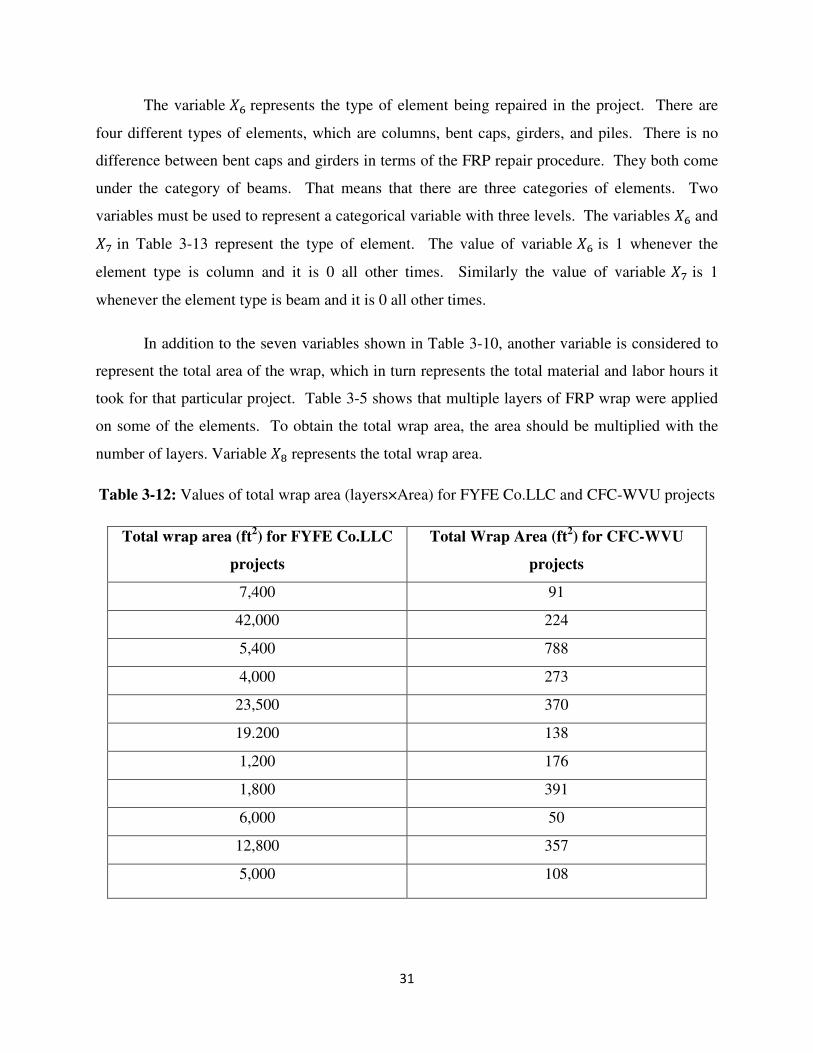
Table 3-12: Values of total wrap area (layers×area) for FYFE Co.LLC and CFC-WVU projects ............ 31
Table 3-13: The setup of variables for regression analysis ......................................................................... 33
Table 4-1: Summary of regression results on columns and girders ............................................................ 35
Table 4-2: Predicted values and residuals of all contract values ................................................................ 36
Table 4-3: The contract values that have element type ‘column’ ............................................................... 37
Table 4-4: Summary of regression results for values with common element type ‘columns’ .................... 38
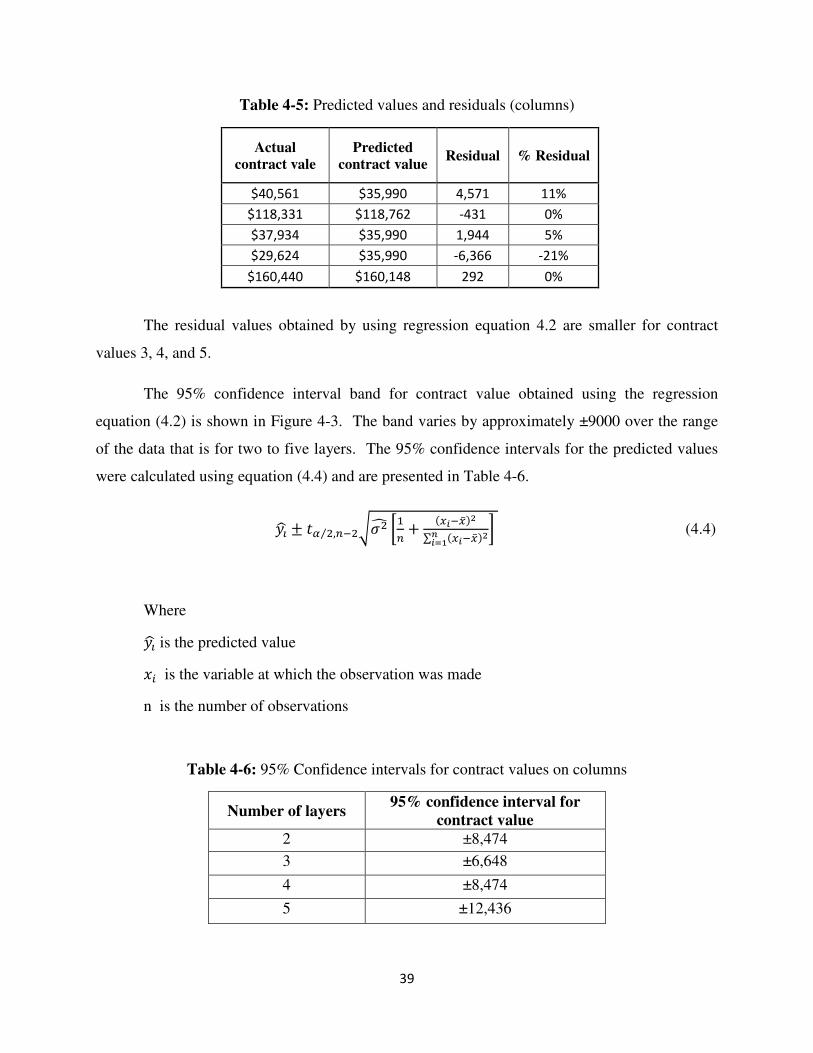
Table 4-5: Predicted values and residuals (columns) .................................................................................. 39
Table 4-6: 95% Confidence intervals for contract values on columns ....................................................... 39
Table 4-7: Data for beam element (girder and caps)................................................................................... 40
Table 4-8: Summary of regression results for values with common element type ‘girder’ ........................ 41
Table 4-9: Predicted values and residuals for beams (girders and caps) .................................................... 42
Table 4-10: Contract values that have element type ‘pile’ ......................................................................... 43
Table 4-11: Summary of results .................................................................................................................. 44
Table 5-1: Predicted values and residuals from regression analysis of all values ...................................... 45

vii
Table 5-2: Predicted values and residuals (columns) .................................................................................. 46
Table 5-3: Predicted values and residuals (girders) .................................................................................... 47
viii
LIST OF ACRONYMS
West Virginia Division of Highways WVDOH
West Virginia Parkways Economic Development and Tourism Authority WVPEDTA
West Virginia Department of Transportation WV DOT
Federal Highway Administration FHWA
Fiber Reinforced Polymer FRP
Reinforced Concrete RC
Life Cycle Cost Analysis LCCA
Polyacrylonitrile PAN
Resin Transfer Molding RTM
Glass Fiber Reinforced Polymer GFRP
Carbon Fiber Reinforced Polymer CFRP
South Branch Valley Railroad SBVR
Steel Reinforced Concrete SRC
1
CHAPTER 1
INTRODUCTION
1.1 Introduction
The state of West Virginia has 7,349 bridges open to public traffic. Most of these bridges
(99%) are owned by West Virginia Division of Highways (WVDOH), and the remaining bridges
are owned by the West Virginia Parkways Economic Development and Tourism Authority
(WVPEDTA) and private owners (WV DOT, 2010). About 37% of these bridges show
significant deterioration either structurally or functionally (keepwvmoving, 2010). Similarly, a
study conducted by the Federal Highway Administration (FHWA) on the condition of the
bridges in the US reported that, 29% of the 587,755 bridges are either functionally or structurally
deficient (Halvard E. Nystrom, 2003). This report estimated that $87.3 billion will be required to
rehabilitate all the deficient bridges in the US. This signifies the importance of finding more
economically viable alternative bridge rehabilitation techniques.
1.1.1 Rehabilitation Methods
There are a wide variety of bridge rehabilitation techniques available. Some of the
techniques are:
• Concrete jacketing
• Steel jacketing
• Steel plate bonding
• FRP wrapping
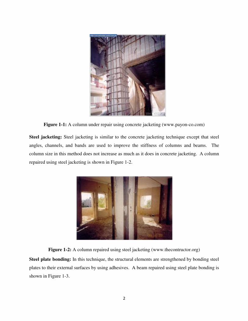
Concrete jacketing: Concrete jacketing involves enlargement of the existing structural members
by placing reinforcing steel rebars around its periphery and then concreting it. Figure 1-1 shows
a column under repair using concrete jacketing.
2
Figure 1-1: A column under repair using concrete jacketing (www.payon-co.com)
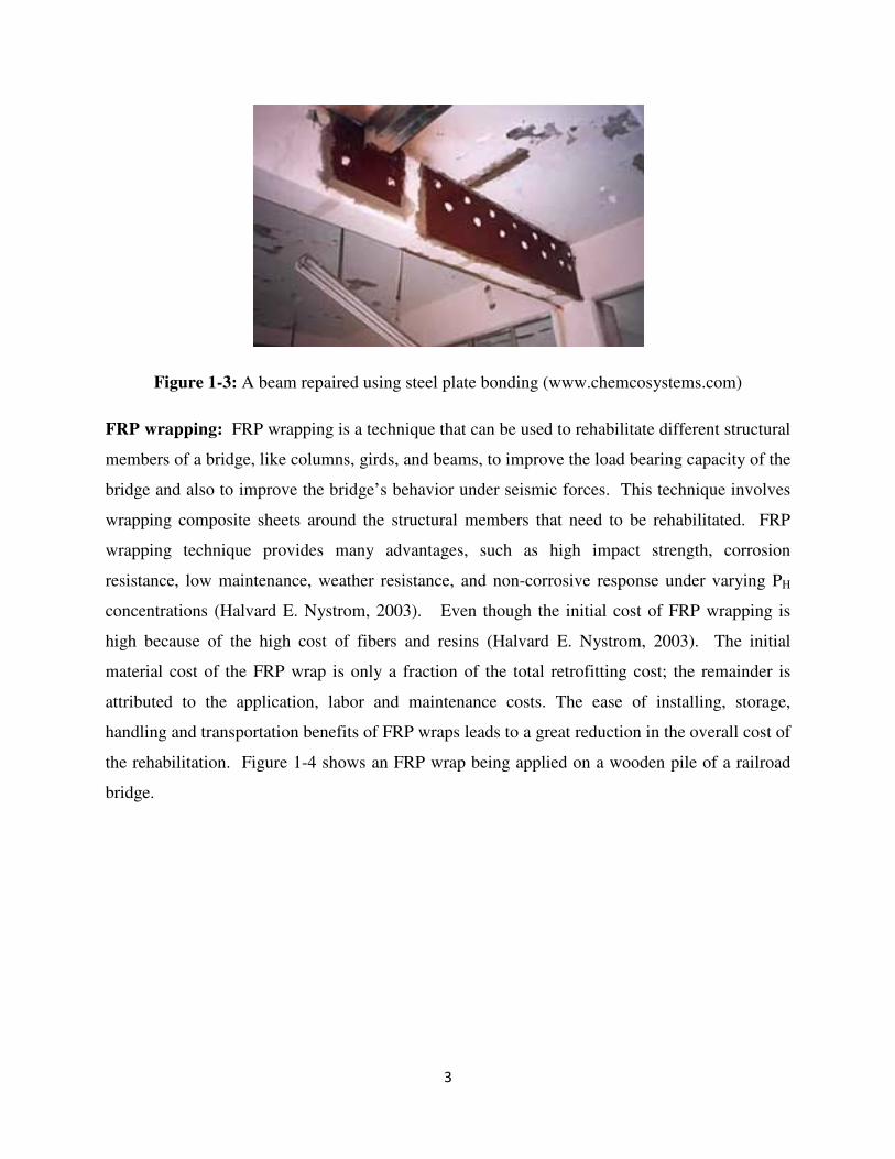
Steel jacketing: Steel jacketing is similar to the concrete jacketing technique except that steel
angles, channels, and bands are used to improve the stiffness of columns and beams. The
column size in this method does not increase as much as it does in concrete jacketing. A column
repaired using steel jacketing is shown in Figure 1-2.
Figure 1-2: A column repaired using steel jacketing (www.thecontructor.org)
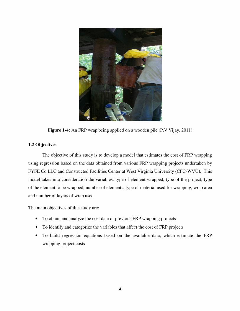
Steel plate bonding: In this technique, the structural elements are strengthened by bonding steel
plates to their external surfaces by using adhesives. A beam repaired using steel plate bonding is
shown in Figure 1-3.
3
Figure 1-3: A beam repaired using steel plate bonding (www.chemcosystems.com)
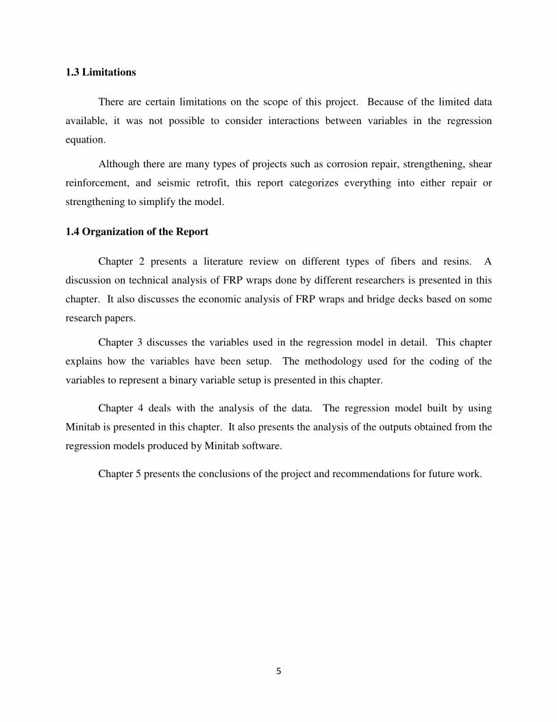
FRP wrapping: FRP wrapping is a technique that can be used to rehabilitate different structural
members of a bridge, like columns, girds, and beams, to improve the load bearing capacity of the
bridge and also to improve the bridge’s behavior under seismic forces. This technique involves
wrapping composite sheets around the structural members that need to be rehabilitated. FRP
wrapping technique provides many advantages, such as high impact strength, corrosion
resistance, low maintenance, weather resistance, and non-corrosive response under varying PH
concentrations (Halvard E. Nystrom, 2003). Even though the initial cost of FRP wrapping is
high because of the high cost of fibers and resins (Halvard E. Nystrom, 2003). The initial
material cost of the FRP wrap is only a fraction of the total retrofitting cost; the remainder is
attributed to the application, labor and maintenance costs. The ease of installing, storage,
handling and transportation benefits of FRP wraps leads to a great reduction in the overall cost of
the rehabilitation. Figure 1-4 shows an FRP wrap being applied on a wooden pile of a railroad
bridge.
4
Figure 1-4: An FRP wrap being applied on a wooden pile (P.V.Vijay, 2011)
1.2 Objectives
The objective of this study is to develop a model that estimates the cost of FRP wrapping
using regression based on the data obtained from various FRP wrapping projects undertaken by
FYFE Co.LLC and Constructed Facilities Center at West Virginia University (CFC-WVU). This
model takes into consideration the variables: type of element wrapped, type of the project, type
of the element to be wrapped, number of elements, type of material used for wrapping, wrap area
and number of layers of wrap used.
The main objectives of this study are:
• To obtain and analyze the cost data of previous FRP wrapping projects
• To identify and categorize the variables that affect the cost of FRP projects
• To build regression equations based on the available data, which estimate the FRP
wrapping project costs
5
1.3 Limitations
There are certain limitations on the scope of this project. Because of the limited data
available, it was not possible to consider interactions between variables in the regression
equation.
Although there are many types of projects such as corrosion repair, strengthening, shear
reinforcement, and seismic retrofit, this report categorizes everything into either repair or
strengthening to simplify the model.
1.4 Organization of the Report
Chapter 2 presents a literature review on different types of fibers and resins. A
discussion on technical analysis of FRP wraps done by different researchers is presented in this
chapter. It also discusses the economic analysis of FRP wraps and bridge decks based on some
research papers.
Chapter 3 discusses the variables used in the regression model in detail. This chapter
explains how the variables have been setup. The methodology used for the coding of the
variables to represent a binary variable setup is presented in this chapter.
Chapter 4 deals with the analysis of the data. The regression model built by using
Minitab is presented in this chapter. It also presents the analysis of the outputs obtained from the
regression models produced by Minitab software.
Chapter 5 presents the conclusions of the project and recommendations for future work.
6
CHAPTER 2
BACKGROUND AND LITERATURE REVIEW
A thorough literature search was done using the World Wide Web, West Virginia
University library’s databases and West Virginia Department of Transportation (WVDOT) for
the cost information of FRP wraps. Many reports on the Life Cycle Cost Analysis (LCCA) of
FRP bridge decks were found. The literature found on the LCCA was on FRP decks and not on
FRP wraps. A significant amount of information was found on the technical details of FRP
wraps but not on their cost information. All cost information found on the FRP wraps is
mentioned in subsequent sections of this chapter.
2.1 Background
2.1.1 Fiber Reinforced Polymers (FRP)
Fiber Reinforced Polymer (FRP) is a composite material. Composites can be defined as a
combination of two or more materials that do not interact chemically with each other, such that
the properties (strength, durability, etc.) of the combination are better than that of the individual
constituents (Wilde, 1988). Usually there are two kinds of materials that are used in FRP wraps:
fibers and matrices. Most commonly used fibers are glass fibers, carbon fibers and, aramid
fibers. Most commonly used matrix types are thermoplastic polymers and thermosetting
polymers. Usually polyester, vinyl ester and epoxy are used as matrices. The durability of the
FRP is a function of both the fiber and the matrix, which makes it more durable than fiber alone.
The strength in FRP is achieved primarily by the fiber; it makes FRP materials stronger in
tension.
2.1.1.1 Fibers
The three main types of fibers are glass, carbon, and aramid fibers. Glass fibers are
mostly used in engineering applications because of their availability and good mechanical
properties. Based on their properties, glass fibers are categorized into three classes: E-class, C-
class, and S-class. E-class was developed for electrical applications, and can be used as an
insulator. S-class has higher strength than E-class (25% more tensile strength) and has good
corrosion properties. C-class fibers are used in preventing corrosion attacks. The other glass
7
fibers which are infrequently used are D-glass, AR-glass, and ECR-glass. The chemical and
electrical properties of different glass fibers are shown in Table 2-1. The physical properties of
glass fibers are shown in Table 2-2.
Table 2-1: Material properties of glass fibers (David Hartman, 1996)
(http://www.agy.com/technical_info/graphics_PDFs/HighStrengthTechPaperEng.pdf)
A GLASS C GLASS D GLASS E GLASS ECRGLAS® AR GLASS R GLASS S-2 GLASS®
Durability (% weight loss)
H 2 O: 24hr 1.8 1.1 0.7 0.7 0.6 0.7 0.4 0.5
168 hr 4.7 2.9 5.7 0.9 0.7 1.4 0.6 0.7
10% HCl: 24 hr 1.4 4.1 21.6 42.0 5.4 2.5 9.5 3.8
168 hr 7.5 21.8 43.0 7.7 3.0 10.2 5.1
10% H 2 SO 4 : 24hr 0.4 2.2 18.6 39.0 6.2 1.3 9.9 4.1
168 hr 2.3 4.9 19.5 42.0 10.4 5.4 10.9 5.7
10% Na 2 CO 3 : 24hr 24.0 13.6 2.1 1.3 3.0 2.0
168 hr 31.0 36.3 2.1 1.8 1.5 2.1
Dielectric Constant 1MH: 6.2 6.9 3.8 6.6 6.9 8.1 6.4 5.3
10 GHz 4.0 6.1 7.0 5.2
Dissipation Factor 1MH: 0.0085 0.0005 0.0025 0.0028 0.0034 0.002
10 GHz 0.0026 0.0038 0.0031 0.0051 0.0068
Volume Resistivity (ohm-cm) 1.0E+10 4.02E+14 3.84E+14 2.03E+14 9.05E+12
Surface Resistivity (ohms) 4.20E+15 1.16E+16 6.74E+13 8.86E+12
Dielectric Strength (volts/mil) 262 250 274 330
ELECTRICAL PROPERTIES
CHEMICAL PROPERTIES
8
Table 2-2: Physical properties of glass fibers (David Hartman, 1996)
(http://www.agy.com/technical_info/graphics_PDFs/HighStrengthTechPaperEng.pdf)
Carbon fibers are very brittle in nature. They are commercially available in 3 forms, long
and continuous tow, chopped and milled. These fibers can be woven into two-dimensional
fabrics of different styles. Carbon fibers can be manufactured from a variety of materials
including petroleum, coal tar pitch and rayon. Depending upon the materials used, carbon fibers
are classified into many types such as Polyacrylonitrile (PAN)-based, pitch-based and rayon-
based fibers. The mechanical properties of some of the carbon fibers are listed in Table 2-3. The
tensile strengths are shown in kilo force per square inch (ksi) and megapascal (105 pascals) units,
whereas tensile modulus values are presented in Gigapascals (GPa). The Msi values represent the
compressive strength of the fiber in Gigapascals.
A GLASS C GLASS D GLASS E GLASS ECRGlas® AR GLASS R GLASS S-2 GLASS®
Density, gm/cc 2.44 2.52 2.11-2.14 2.58 2.72 2.7 2.54 2.46
Refractive Index 1.538 1.533 1.465 1.558 1.579 1.562 1.546 1.521
Softening Point, o
C (o
F) 705 (1300) 750 (1382) 771 (1420) 846 (1555) 882 (1619) 773 (1424) 952 (1745) 1056 (1932)
Annealing Point, o
C (o
F) 588 (1090) 521 (970) 657 (1215) 816 (1500)
Strain Point, o
C (o
F) 522 (1025) 477 (890) 615 (1140) 736 (1357) 766 (1410)
Tensile Strength, MPa
-196 o
C 5380 5310 5310 8275
23 o
C 3310 3310 2415 3445 3445 3241 4135 4890
371 o
C 2620 2165 2930 4445
538 o
C 1725 1725 2140 2415
Young's Modulus, GPa
23 o
C 68.9 68.9 51.7 72.3 80.3 73.1 85.5 86.9
538 o
C 81.3 81.3 88.9
Elongation % 4.8 4.8 4.6 4.8 4.8 4.4 4.8 5.7
PHYSICAL PROPERTIES
Table 2-3: Mechanical properties of carbon fibers
(http://www.corecomposites.com/media/aboutCarbon.pdf
Aramid fibers have great tensile s
resistant applications because of their exclusive proper
point and good fabric integrity at elevated temperatures
polyamides.
2.1.1.2 Matrices
There are three types of matrices
matrix. The use of a matrix
environmental and mechanical attacks
thermoplastic and thermosetting
molecular structure. Thermoplastic polymers are bonded by a weak secondary bond which
breaks down temporarily when heat or pressure is applied, w
called resins) have a strong cross
and provides good electrical and thermal insulation
are nylon and polyethylene. Good examples of thermosetting matrices are epoxy, polyester and
9
Mechanical properties of carbon fibers (corecomposites.com, 2005)
http://www.corecomposites.com/media/aboutCarbon.pdf)
Aramid fibers have great tensile strength and are very flexible. They are
resistant applications because of their exclusive properties like low flammability,
point and good fabric integrity at elevated temperatures. Aramid fibers are made from aromatic
There are three types of matrices available: metal matrix, polymer matrix
atrix is to transfers stresses in fibers and to protect
environmental and mechanical attacks. The polymer matrices are further divided into two types,
matrix. The major difference between these two types is their
Thermoplastic polymers are bonded by a weak secondary bond which
hen heat or pressure is applied, whereas thermosetting polymers (a
strong cross-linked molecular structure which does not br
good electrical and thermal insulation. Good examples of thermoplastic matrices
Good examples of thermosetting matrices are epoxy, polyester and
(corecomposites.com, 2005)
They are used in heat
flammability, high melting
Aramid fibers are made from aromatic
lymer matrix, and ceramic
protect them from
The polymer matrices are further divided into two types,
The major difference between these two types is their
Thermoplastic polymers are bonded by a weak secondary bond which
hereas thermosetting polymers (also
structure which does not break when heated
Good examples of thermoplastic matrices
Good examples of thermosetting matrices are epoxy, polyester and
10
vinyl. Physical and mechanical properties of thermosetting and thermoplastic polymers are
shown in Table 2-4.
Table 2-4: Material properties of thermosetting and thermoplastic polymers (Clyne, 1996)
2.1.2 FRP Manufacturing Methods
FRP structures are manufactured mostly by using automatic methods. Automatic
methods include compression molding, resin transfer molding, and pultrusion. A non-automatic
method known as hand lay-up is also used. Fiber packing in a FRP depends on the method of
manufacturing. The pultrusion process is a highly automated and frequently used technique.
2.1.2.1 Compression Molding
Compression molding involves placing the premix (charge) in the mold. The premix
consists of chopped glass reinforcement and the resin. The premix in the mold is held at high
pressure and then heated to form the FRP structure. Compression molding process is used only
when large quantities of FRPs are needed because of its high cost of tooling.
2.1.2.2 Resin Transfer Molding (RTM)
Resin Transfer Molding (RTM) is similar to compression molding except that only
reinforced polymer is loaded into the closed mold initially. Resin is then injected into the mold
to form the finished part. RTM offers superior surface finishing as the material is completely
enclosed within the mold.
2.1.2.3 Pultrusion
Pultrusion is the frequently used method because it is a continuous process and has the
highest throughput. This process involves sending glass reinforcement of continuous strand mats
into the pultrusion die designed with strict tolerances. The reinforcement is pulled through a
resin bath and then passes through extreme pressure to get rid of any excess air and resin.
Density Young's Poisson's Tensile Failure
(Mg/m3
) modulus (GPa) ratio strength (GPa) strain (%)
Thermoset epoxy resin 1.1-1.4 3.0-6.0 0.38-0.40 0.035-0.1 1.0-6.0
Thermoplastic PEEK 1.26-1.32 3.6 0.3 0.17 50
Matrix
11
2.1.2.4 Hand Lay-up
Hand lay-up is one of the most basic FRP manufacturing processes. It requires applying
each layer of reinforcement and resin manually into an open mold. This process is repeated until
the desired part thickness is achieved.
FRP wrapping is used to increase shear and flexural strengths of structural elements, to
repair damaged surfaces (mainly due to corrosion), and also to provide protection against blast
and seismic forces (seismic retrofitting). FRP wrapping can be used to increase load-bearing
capacities of bridges built with all concrete, steel, and wood members. In addition to these, FRP
wrapping is now being used in strengthening walls, slabs, tubes, and tunnels.
2.1.3 FRP Wrap Manufacturing
The manufacturing of FRP wraps is different when compared to that of FRP structures.
It begins with the manufacturing of the fiber. The raw material used for manufacturing carbon
fibers is polyacrilonytrile, which is made by polymerizing acrylonitrile. This raw material is
drawn into strands before the process begins. The process of manufacturing carbon fiber
involves oxidization, carbonization, and surface preparation of the polacrylonitrile strands. The
strands are oxidized by first heating them to 3000C in air, which breaks the hydrogen bonds and
creates a fireproof material by oxidizing. The strands are then heated between 1,500 and
3,0000C in an inert gas to carbonize them. Carbonization makes the raw material 100% carbon.
Different grades of carbon fibers are made depending upon the temperatures used in
carbonization. To make the fiber bond with epoxies that are used in wraps, the surface of the
fiber is slightly oxidized by immersing it in different gases.
The manufacturing of glass fibers is also a multistep process involving batching, melting,
fiberization and coating. The raw material used in glass fiber manufacturing is silica. In
batching, silica is weighed and mixed with other ingredients like aluminum oxide and
magnesium oxide to improve its properties. The batch is then heated to as high as 14000C to
form molten glass. The molten glass is extruded through very fine orifices to form strands.
These extruded strands then pass through fibrous elements called as filaments. Finally, a
chemical coating is applied on the fiber to protect it from breaking. These fibers are woven into
uni- and bi-directional matrices to make wraps.
12
2.1.4 FRP Wraps – A Historical View
The US requires as much as $87.3 billion dollars to rehabilitate 29% of the 587,755 (i.e.
170,449) deficient bridges in the country (Halvard E. Nystrom, 2003). The main reason for
bridge elements deterioration is corrosion. Because of the de-icing salts being applied on the
bridge decks during winter, the steel in reinforced concrete columns gets corroded. Since the use
of deicing salts is inevitable, it has become crucial to find an effective, yet financially viable,
way of dealing with corrosion. The most popular ways of preventing corrosion are:
• Physically disrupting the chlorides from reaching steel surface
• Making the surface of a concrete structure less corrosive by using admixtures and
inhibitors
• Using a reinforcement resistant to corrosion by using alloys
• Using electrochemical methods to reduce chloride effects
FRP wrapping works as a physical barrier between chlorides and the steel surface. In
wooden bridges, FRP wrapping was found to be more economical than replacing the whole pier
(Lopez-Anido. A, 2002) .
The first major civil construction with FRP was the Ulenbergstrasse Bridge in
Dusseldorf, Germany. It is a 154-foot-long GFRP bridge built in 1987 (Clarke, 1998). FRPs are
being used in aerospace, marine, and automotive industries.
FRP wraps are used to increase flexural capacities, to improve shear capacity and to
increase the ductility of concrete load-bearing members. The first two applications depend upon
the bond between the concrete and the FRP. As the transfer of stresses between concrete and
FRP is very critical, they are called “Bond critical”. The third application, i.e., increasing the
ductility of load-bearing members, is called “contact critical”, because the contact that keeps the
beam confined is critical (Brown, 2005).
Figure 2-1 shows examples of flexural and shear strengthening. The wrap is applied
along the element’s longitudinal axis and cross section to increase flexural strength and shear
strengths respectively. An example of contact critical application (column wrapping) is shown in
13
Figure 2-2. Column wrapping is done to protect the column from environmental corrosion and
also to increase its strength.
Figure 2-1: Flexural and shear strengthening of beams
Figure 2-2: Example of contact critical application (column wrapping)
2.2 Literature review
A lot of research is going on in the area of FRP wrapping in terms of its application to
different civil infrastructures.
In a research report titled “Effect of Wrapping Chloride Contaminated Structural
Concrete with Multiple Layers of Glass Fiber Composites and Resin” prepared for the Texas
Department of Transportation, the authors (C. L. Shoemaker, 2001) performed laboratory
experiments to understand the effects of FRP wraps in preventing corrosion. Thirteen specimens
(7 of them were wrapped with GFRP) were exposed to a corrosive environment in an exposure
14
tank. The wrapping was done on the entire length of the specimens except the lower one foot.
They placed the specimens in a row in an exposure tank where a 3.5% saline solution was
introduced for a week to intentionally expedite the process of corrosion. Following the wet
period they left the exposure tank dry for another two weeks. The results have shown that the
wrapped columns were well below 95% probability of corrosion. The unwrapped portions of the
specimens had 0.1 to 0.4% chloride content, whereas the wrapped portions of specimens had
only 0.03%. The amount of chloride present in the column prior to wrapping reduced the
wrapping effect.
A business organization called “Air Logistics Corporation” published a paper titled
“Analysis of Aquawrap for use in repairing damaged pipelines” (Worth, 2005) presenting all the
test results done on its proprietary product called Aquawrap. Aquawrap is comprised of
proprietary polyurethane resin and bi-axial glass fiber which is water activated. Aquawrap can
be used to repair pipelines and cylindrical objects of metal and concrete. A number of tests were
done on the Aquawraps including tension, flexural and compressive strengths, burst strength,
flammability, adhesion to the steel surfaces, soaking under alkaline solutions tests, and impact
tests. All of the test results showed that Aquawrap was reliable and efficient in terms of its use
in repairing damaged pipelines due to corrosion.
In another research report titled “Durability of Fiber Reinforced Polymer and External
FRP-Concrete Bond” the authors (Homam, 2000) subjected 252 wrapped and unwrapped
concrete cylinders (75-mm in diameter and 150 mm long) to various environmental conditions
such as freeze-thaw cycles, UV radiation, temperature variation, and NaOH with varying PH
concentrations (10,12 and 13.7). Both CFRP and GFRP were tested. Durability of FRP-concrete
bond has also been studied on 264 specimens made by casting two halves together and
reinforcing them with 25×262.5-mm FRP laminates. All the specimens were moist cured for 28
days. All the specimens (unwrapped and wrapped with CFRP and GFRP) were subjected to
monotonic compression and axial stress, strain values were recorded. Both CFRP and GFRP
wrapped specimens were ductile, but the yield point was almost equal to that of unwrapped
columns. Each extra layer of CFRP increased the compressive strength by 80%, whereas GFRP
showed a 30-40% increase in strength. After exposing the specimens to 300 freeze thaw cycles,
the strength of unwrapped specimens dropped by about 15-20% compared with the wrapped
15
ones. The specimens (both CFRP and GFRP) used to study the FRP concrete bonding showed
only a small drop in lap-shear strength.
The effects of using FRP wraps on wood piles were discussed in a paper titled
“Experimental characterization of FRP Composite-Wood pile structural response by bending
tests.” The authors (Lopez-Anido.A, P. Micheal and T.C. Sandford, 2002) developed and tested
two types of load transfer mechanisms. One is a cement based structural grout and the other is
steel shear connectors with polyurethene grout. The authors damaged three specimens each nine
meters long, by reducing 60% of the cross sectional area. The reference wood pile was subjected
to a bending test intact (undamaged) initially. Then two uni-directional GFRP (weight 880 g/m2,
thickness 3.3 mm) wraps were applied around each of the piles. Both the piles were subjected to
a three point bending test and both load transfer mechanisms were studied. The load was applied
in cycles and the maximum load was anticipated using the beam structural model. The peak load
achieved by the intact pile was 79 kN before it failed. The pre-damaged control pile’s peak load
was 8.2 kN. The pre-damaged pile with GFRP and cement grout achieved a peak load of 115
kN, whereas the one with GFRP and polyurethene grout achieved only 52 kN peak load. The
authors concluded that polyurethene grout was not able to completely restore the bending
capacity, but it can be used for marine borer protection where wood damage is not critical.
The economic aspects of FRP wrapping on rail road bridges was discussed in a paper
titled “Rapid restoration of railroad timber bridges using polymer composites” by the authors
(P.V.Vijay, GangaRao H.V.S,Ruifeng Liang, Mark Skidmore 2011). GFRP (E-Glass) composite
wraps were used to rapidly rehabilitate damaged wood piles of 11 timber railroad bridges on
South Branch Valley Railroad (SBVR). The eleven bridges consisted of 57 wooden piles. The
project took 562 man hours to wrap approximately 1500 ft2 of GFRP on these 57 wooden piles.
Some of these piles were submerged in water, so cofferdams were built using sandbags and
water was pumped out. A torpedo-type heater was used to dry out the submerged part of the
piles. Most of the piles were decayed at ground level, so the soil around them was dug up. A
wire brush was used to clean the outside debris on the piles, and the piles were then sanded. The
areas to be wrapped were pre-coated G1149 resin to prime the surface. After priming, the piles
were wrapped with phenolic soaked GFRP wraps with a length of twice the circumference of the
pile to achieve 2 layers of wrapping. The excavation and pile preparation task shown in Figure
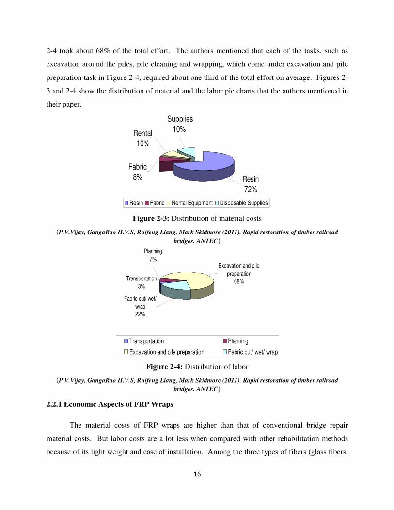
16
2-4 took about 68% of the total effort. The authors mentioned that each of the tasks, such as
excavation around the piles, pile cleaning and wrapping, which come under excavation and pile
preparation task in Figure 2-4, required about one third of the total effort on average. Figures 2-
3 and 2-4 show the distribution of material and the labor pie charts that the authors mentioned in
their paper.
Figure 2-3: Distribution of material costs
(P.V.Vijay, GangaRao H.V.S, Ruifeng Liang, Mark Skidmore (2011). Rapid restoration of timber railroad
bridges. ANTEC)
Figure 2-4: Distribution of labor
(P.V.Vijay, GangaRao H.V.S, Ruifeng Liang, Mark Skidmore (2011). Rapid restoration of timber railroad
bridges. ANTEC)
2.2.1 Economic Aspects of FRP Wraps
The material costs of FRP wraps are higher than that of conventional bridge repair
material costs. But labor costs are a lot less when compared with other rehabilitation methods
because of its light weight and ease of installation. Among the three types of fibers (glass fibers,
Resin
72%
Fabric
8%
Rental
10%
Supplies
10%
Resin Fabric Rental Equipment Disposable Supplies
Excavation and pile
preparation
68%
Planning
7%
Transportation
3%
Fabric cut/ wet/
wrap
22%
Transportation Planning
Excavation and pile preparation Fabric cut/ wet/ wrap
17
aramid fibers, and carbon fibers) available, glass fibers are known as low cost fibers, aramid
fibers are medium cost fibers and carbon fibers are high cost and high performance fibers. FRP
wraps have become very popular because of their ease of installation and reduced labor costs.
Three to four columns can be wrapped in a day on average. Some reports say that the average
cost of rehabilitation or replacement of a bridge is as high as $2 to $8 billion per bridge (Lopez-
Anido, 2001).
2.2.2 Review of Previous Models
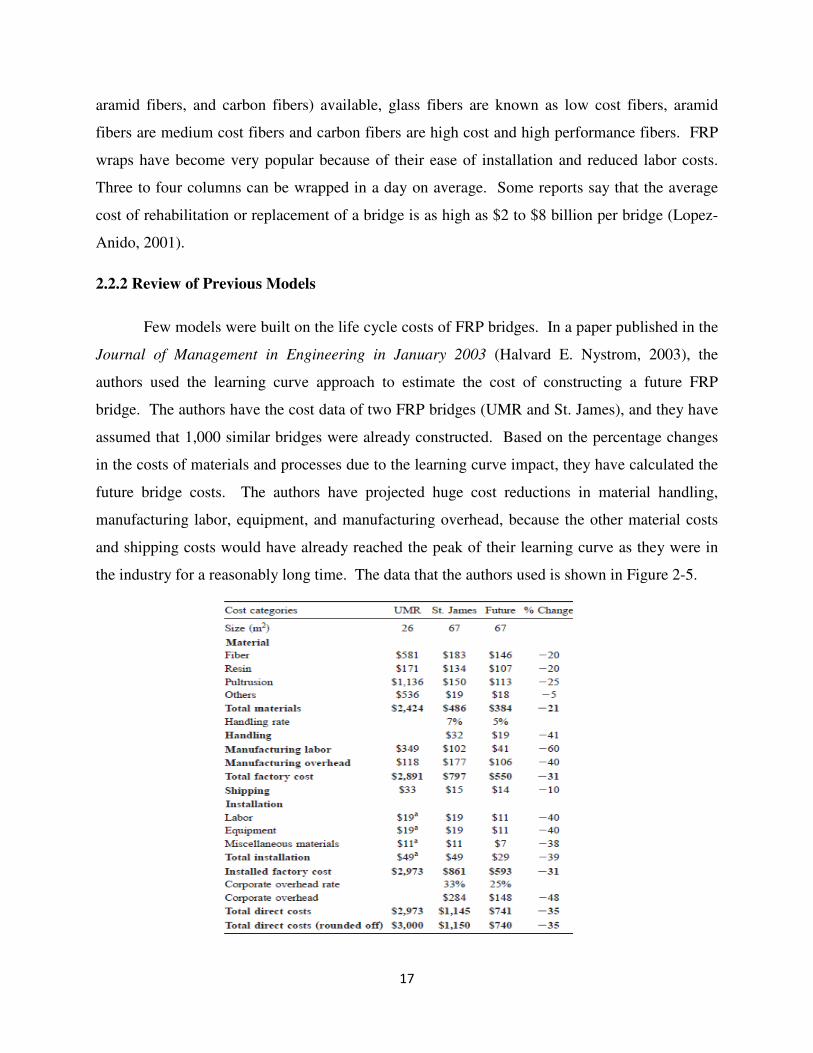
Few models were built on the life cycle costs of FRP bridges. In a paper published in the
Journal of Management in Engineering in January 2003 (Halvard E. Nystrom, 2003), the
authors used the learning curve approach to estimate the cost of constructing a future FRP
bridge. The authors have the cost data of two FRP bridges (UMR and St. James), and they have
assumed that 1,000 similar bridges were already constructed. Based on the percentage changes
in the costs of materials and processes due to the learning curve impact, they have calculated the
future bridge costs. The authors have projected huge cost reductions in material handling,
manufacturing labor, equipment, and manufacturing overhead, because the other material costs
and shipping costs would have already reached the peak of their learning curve as they were in
the industry for a reasonably long time. The data that the authors used is shown in Figure 2-5.
18
Figure 2-5: Cost data of UMR and St. James bridges (Halvard E. Nystrom, 2003)
In another life cycle cost estimation approach done by a graduate student in the Industrial
Engineering Department of West Virginia University (Roychoudhury, 2001), the initial
construction costs were inputted by the user. The per square foot cost of FRP deck fabrication
was provided by the user, and the initial construction costs were calculated based upon the length
of the bridge.
In the learning curve approach model based on the assumptions the authors have made,
the future bridge would cost 40-60% less in installation, labor and overhead costs compared to
the previously built bridges. Since the authors (Halvard E. Nystrom, 2003) have the cost data of
only two bridges, they have assumed that 1,000 bridges were already built and came up with
those percentages.
The initial costs of FRP bridge deck include manufacturing cost, transportation cost and
erection cost. The initial costs of FRP bridge decks are expected to be higher than the Steel
Reinforced Concrete (SRC). The weight of the FRP bridge deck is approximately 20-25% that
of Steel Reinforced Concrete deck (Sahirman, 2009).
19
CHAPTER 3
METHODOLOGY
The basic rehabilitation operations that are done on different structural elements are
strengthening, repair, and retrofitting. Seismic retrofitting is also a strengthening operation
except that it is done on the structures present in seismically active areas. The different
strengthening, retrofitting and repair operations that can be done on structural elements and the
structural elements suitable for those operations are listed below
• Strengthening Operations
Flexural strengthening (beams, slabs, walls, etc.)
Shear strengthening (beams, columns, walls, etc.)
Axial strengthening (Columns, pressure vessels, etc.)
• Retrofitting
Shear retrofitting (beams, columns, walls, joints)
Confinement (beams, columns, joints)
• Repair/Rehabilitation
Corrosion repair (columns, beams)
All of these operations can be done on both reinforced concrete and timber structural members.
3.1 FRP Application Procedure
The step- by-step procedure for FRP application usually followed is
Step 1: Surface preparation
Step 2: Installation of FRP wrap
Step 3: Non-Destructive Testing (NDT)

20
3.1.1 Surface Preparation
Any bridge element to be wrapped should first be prepared for a successful installation.
Surface preparation involves removal of the debris, cleaning the dust and filling the gaps on the
surface with an appropriate material. Anti-chloride chemicals must be used to remove the
chloride content that is already present on the surface. The surface must be cleaned by sand
blasting and by using pressurized air to make it as smooth as possible. The damaged surface
should be brought back to its original shape by adding material.
3.1.2 Installation of FRP Wrap
After the surface preparation, a layer of primer is applied on the repair area of the
element. The required numbers of FRP wraps are then wrapped to the bridge element and any
air bubbles formed are removed by pressing them against the element by hand. The FRP is then
dried and coated with paint before a glossy film forms on the surface of FRP.
3.1.3 Non-Destructive Testing (NDT)
Non-Destructive Testing is done on the bridge element to evaluate the bonding between
the FRP wrap and the surface of the element. The different types of NDT techniques include
infrared thermography, optical holographic NDT and microwave sensor techniques.
Every rehabilitation project involves man hours for surface preparation, FRP application,
handling materials, machines, and NDT evaluation. These are considered as cost items. The
other miscellaneous cost items are transportation and disposable supplies costs. The total
contract value is an aggregate of the material, man-hours, equipment, transportation, profits and
overhead costs. A regression model is developed in later sections of this chapter using the total
contract values of different FRP wrapping projects.
21
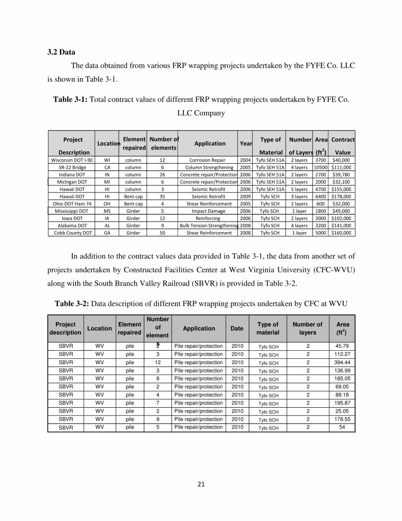
3.2 Data
The data obtained from various FRP wrapping projects undertaken by the FYFE Co. LLC
is shown in Table 3-1.
Table 3-1: Total contract values of different FRP wrapping projects undertaken by FYFE Co.
LLC Company
In addition to the contract values data provided in Table 3-1, the data from another set of
projects undertaken by Constructed Facilities Center at West Virginia University (CFC-WVU)
along with the South Branch Valley Railroad (SBVR) is provided in Table 3-2.
Table 3-2: Data description of different FRP wrapping projects undertaken by CFC at WVU
SBVR WV pile 2 Pile repair/protection 2010 Tyfo SCH 2 45.79
SBVR WV pile 3 Pile repair/protection 2010 Tyfo SCH 2 112.27
SBVR WV pile 12 Pile repair/protection 2010 Tyfo SCH 2 394.44
SBVR WV pile 3 Pile repair/protection 2010 Tyfo SCH 2 136.99
SBVR WV pile 8 Pile repair/protection 2010 Tyfo SCH 2 185.05
SBVR WV pile 2 Pile repair/protection 2010 Tyfo SCH 2 69.05
SBVR WV pile 4 Pile repair/protection 2010 Tyfo SCH 2 88.18
SBVR WV pile 7 Pile repair/protection 2010 Tyfo SCH 2 195.87
SBVR WV pile 2 Pile repair/protection 2010 Tyfo SCH 2 25.05
SBVR WV pile 9 Pile repair/protection 2010 Tyfo SCH 2 178.55
SBVR WV pile 5 Pile repair/protection 2010 Tyfo SCH 2 54
DateType of
material
Number of
layers
Element
repaired
Number
of
element s
Area
(ft2)
Location ApplicationProject
description
Project Type of Number Area Contract
Description Material of Layers (ft2) Value
Wisconsin DOT I-90 WI column 12 Corrosion Repair 2004 Tyfo SEH 51A 2 layers 3700 $40,000 SR-22 Bridge CA column 6 Column Strengthening 2005 Tyfo SEH 51A 4 layers 10500 $111,000
Indiana DOT IN column 26 Concrete repair/Protection 2006 Tyfo SEH 51A 2 layers 2700 $39,780 Michigan DOT MI column 6 Concrete repair/Protection 2006 Tyfo SEH 51A 2 layers 2000 $32,100
Hawaii DOT HI column 3 Seismic Retrofit 2006 Tyfo SEH 51A 5 layers 4700 $155,000
Hawaii DOT HI Bent cap 35 Seismic Retrofit 2009 Tyfo SCH 3 layers 6400 $178,000
Ohio DOT Ham 74 OH Bent cap 4 Shear Reinforcement 2005 Tyfo SCH 2 layers 600 $32,000 Mississippi DOT MS Girder 5 Impact Damage 2006 Tyfo SCH 1 layer 1800 $49,000
Iowa DOT IA Girder 12 Reinforcing 2006 Tyfo SCH 2 layers 3000 $102,000
Alabama DOT AL Girder 9 Bulb Tension Strengthening 2008 Tyfo SCH 4 layers 3200 $141,000
Cobb County DOT GA Girder 50 Shear Reinforcement 2008 Tyfo SCH 1 layer 5000 $160,000
LocationNumber of
elementsApplication Year
Element
repaired
22
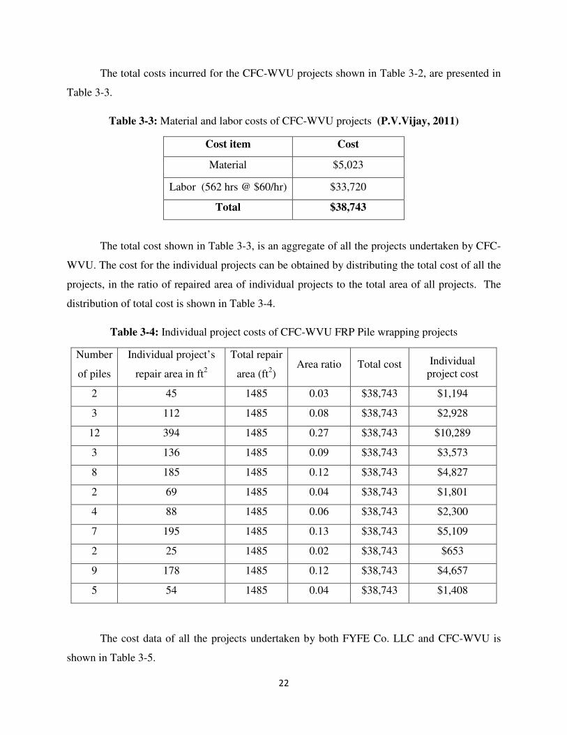
The total costs incurred for the CFC-WVU projects shown in Table 3-2, are presented in
Table 3-3.
Table 3-3: Material and labor costs of CFC-WVU projects (P.V.Vijay, 2011)
Cost item Cost
Material $5,023
Labor (562 hrs @ $60/hr) $33,720
Total $38,743
The total cost shown in Table 3-3, is an aggregate of all the projects undertaken by CFC-
WVU. The cost for the individual projects can be obtained by distributing the total cost of all the
projects, in the ratio of repaired area of individual projects to the total area of all projects. The
distribution of total cost is shown in Table 3-4.
Table 3-4: Individual project costs of CFC-WVU FRP Pile wrapping projects
Number
of piles
Individual project’s
repair area in ft2
Total repair
area (ft2) Area ratio Total cost Individual
project cost
2 45 1485 0.03 $38,743 $1,194
3 112 1485 0.08 $38,743 $2,928
12 394 1485 0.27 $38,743 $10,289
3 136 1485 0.09 $38,743 $3,573
8 185 1485 0.12 $38,743 $4,827
2 69 1485 0.04 $38,743 $1,801
4 88 1485 0.06 $38,743 $2,300
7 195 1485 0.13 $38,743 $5,109
2 25 1485 0.02 $38,743 $653
9 178 1485 0.12 $38,743 $4,657
5 54 1485 0.04 $38,743 $1,408
The cost data of all the projects undertaken by both FYFE Co. LLC and CFC-WVU is
shown in Table 3-5.
23
Table 3-5: Total contract values of all projects undertaken by both FYFE Co. LLC and CFC-
WVU
* In the Hawaii DOT project done on piles, there are 3 columns and 35 bentcaps. Since the
separate costs for columns and bentcaps are not available, the 3 columns were also considered as
bentcaps.
* The FDOT project was not considered in the analysis because it is the only project done on
wood piles with a contract value of $219,000, whereas other projects on piles were done with
contract values in the range of $1,000-$9,000.
* All the projects undertaken by FYFE Co. LLC (except FDOT) were on the bridge elements
made of concrete, whereas all the projects undertaken by CFC-WVU were on the wood piles.
The variable ‘location’ in Table 3-5 contributes transportation cost to the contract value
for that particular project. The transportation cost represents the transportation cost of the
material to the project site. If the cost of transportation is removed from the contract value, the
variable ‘location’ need not be considered in the regression analysis. There are some
Project Type of Number Area Contract
Description Material of Layers (sft) Value
Wisconsin DOT I-90 WI column 12 Corrosion Repair 2004 Tyfo SEH 51A 2 layers 3,700 $40,000
SR-22 Bridge CA column 6 Column Strengthening 2005 Tyfo SEH 51A 4 layers 10,500 $111,000
Indiana DOT IN column 26 Concrete repair/Protection 2006 Tyfo SEH 51A 2 layers 2,700 $39,780
Michigan DOT MI column 6 Concrete repair/Protection 2006 Tyfo SEH 51A 2 layers 2,000 $32,100
Hawaii DOT HI column 3 Seismic Retrofit 2006 Tyfo SEH 51A 5 layers 4,700 $155,000
FDOT* FL Pile 16 Corrosion Protection 2008 Tyfo SEH 51A 3 layers 5,500 $219,000
Hawaii DOT* HI Bent cap 38 Seismic Retrofit 2009 Tyfo SCH 3 layers 6,400 $178,000
Ohio DOT Ham 74 OH Bent cap 4 Shear Reinforcement 2005 Tyfo SCH 2 layers 600 $32,000
Mississippi DOT MS Girder 5 Impact Damage 2006 Tyfo SCH 1 layer 1,800 $49,000
Iowa DOT IA Girder 12 Reinforcing 2006 Tyfo SCH 2 layers 3,000 $102,000
Alabama DOT AL Girder 9 Bulb Tension Strengthening 2008 Tyfo SCH 4 layers 3,200 $141,000
Cobb County DOT GA Girder 50 Shear Reinforcement 2008 Tyfo SCH 1 layer 5,000 $160,000
SBVR WV pile 2 Pile repair/protection 2010 Tyfo SCH 2 46 $1,194
SBVR WV pile 3 Pile repair/protection 2010 Tyfo SCH 2 112 $2,928
SBVR WV pile 12 Pile repair/protection 2010 Tyfo SCH 2 394 $10,289
SBVR WV pile 3 Pile repair/protection 2010 Tyfo SCH 2 137 $3,573
SBVR WV pile 8 Pile repair/protection 2010 Tyfo SCH 2 185 $4,827
SBVR WV pile 2 Pile repair/protection 2010 Tyfo SCH 2 69 $1,801
SBVR WV pile 4 Pile repair/protection 2010 Tyfo SCH 2 88 $2,300
SBVR WV pile 7 Pile repair/protection 2010 Tyfo SCH 2 196 $5,109
SBVR WV pile 2 Pile repair/protection 2010 Tyfo SCH 2 25 $653
SBVR WV pile 9 Pile repair/protection 2010 Tyfo SCH 2 179 $4,657
SBVR WV pile 5 Pile repair/protection 2010 Tyfo SCH 2 54 $1,408
LocationNumber of
elementsApplication Year
Element
repaired
24
assumptions made in calculating transportation material costs for projects undertaken by both
FYFE Co. LLC and CFC-WVU, they are:
1) The cost of material transportation is assumed to be $1 per 2,500 lbs. per mile.
2) The average distance travelled for the projects undertaken by FYFE Co. LLC is assumed
to be 400 miles for all the projects.
3) The weight of the wrap is assumed to be 0.5 lbs. per layer of FRP wrap per square foot.
4) The assumed man hours spent on transportation for FYFE Co. LLC projects are shown in
Table 3-6
5) The labor rate for FYFE Co. LLC projects was assumed to be $100/hr, whereas for the
projects done by CFC-WVU the labor rate was assumed to be $60/hr.
Table 3-6: Estimated Man hours spent on labor transportation for the projects done by FYFE Co.
LLC
Project location Man hours spent on labor transportation
Wisconsin 48
California 32
Indiana 48
Michigan 48
Hawaii 70
Hawaii 70
Ohio 32
Mississippi 70
Iowa 70
Alabama 70
Georgia 48
The transportation costs for projects done by both FYFE Co. LLC and CFC-WVU are
shown in Tables 3-7 and 3-8 respectively.
25
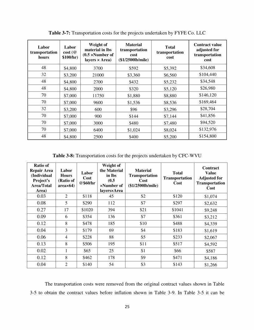
Table 3-7: Transportation costs for the projects undertaken by FYFE Co. LLC
Labor transportation
hours
Labor cost (@ $100/hr)
Weight of material in lbs
(0.5 ×Number of layers × Area)
Material transportation
cost ($1/2500lb/mile)
Total transportation
cost
Contract value adjusted for
transportation cost
48 $4,800 3700 $592 $5,392 $34,608
32 $3,200 21000 $3,360 $6,560 $104,440
48 $4,800 2700 $432 $5,232 $34,548
48 $4,800 2000 $320 $5,120 $26,980
70 $7,000 11750 $1,880 $8,880 $146,120
70 $7,000 9600 $1,536 $8,536 $169,464
32 $3,200 600 $96 $3,296 $28,704
70 $7,000 900 $144 $7,144 $41,856
70 $7,000 3000 $480 $7,480 $94,520
70 $7,000 6400 $1,024 $8,024 $132,976
48 $4,800 2500 $400 $5,200 $154,800
Table 3-8: Transportation costs for the projects undertaken by CFC-WVU
Ratio of Repair Area (Individual Project’s
Area/Total Area)
Labor Hours
(Ratio of area×64)
Labor Cost
@$60/hr
Weight of the Material
in lbs (0.5
×Number of layers×Area
Material Transportation
Cost ($1/2500lb/mile)
Total Transportation
Cost
Contract Value
Adjusted for Transportation
Cost
0.03 2 $118 45 $2 $120 $1,074
0.08 5 $290 112 $7 $297 $2,632
0.27 17 $1020 394 $21 $1041 $9,248
0.09 6 $354 136 $7 $361 $3,212
0.12 8 $478 185 $10 $488 $4,339
0.04 3 $179 69 $4 $183 $1,619
0.06 4 $228 88 $5 $233 $2,067
0.13 8 $506 195 $11 $517 $4,592
0.02 1 $65 25 $1 $66 $587
0.12 8 $462 178 $9 $471 $4,186
0.04 2 $140 54 $3 $143 $1,266
The transportation costs were removed from the original contract values shown in Table
3-5 to obtain the contract values before inflation shown in Table 3-9. In Table 3-5 it can be
26
observed that the contracts were undertaken in different years. The contract values were
modified to account for inflation of the dollar. For example, the value of one dollar in 2004 is
not the same as one dollar in 2002. In order to bring equality between contract values in
different years, a base year should be chosen to which all contract values will have to be inflated
to. The year to which the contract values will have to be adjusted is considered to be 2011 so
that the values will be as recent as possible. Table 3-9 shows the actual and inflated contract
values of the projects. The inflation rates were calculated by using the Consumer Price Index
(CPI). Every month, the Bureau of Labor Statistics (BLS) releases CPI value. The inflation rate
of a particular year can be calculated by using the formula
�������� ��� = ���� � × 100 (3.1)
Where
B = CPI value in 2011(January)
A = CPI value of the year in which contract was done
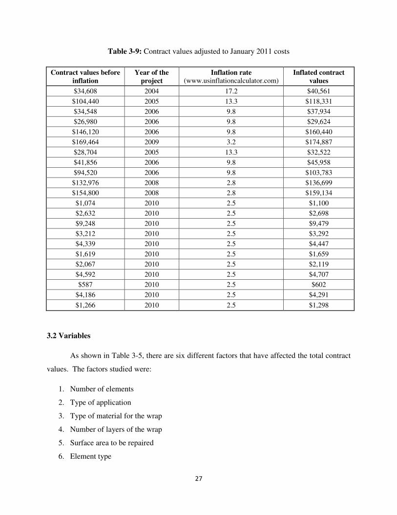
27
Table 3-9: Contract values adjusted to January 2011 costs
Contract values before inflation
Year of the project
Inflation rate (www.usinflationcalculator.com)
Inflated contract values
$34,608 2004 17.2 $40,561
$104,440 2005 13.3 $118,331
$34,548 2006 9.8 $37,934
$26,980 2006 9.8 $29,624
$146,120 2006 9.8 $160,440
$169,464 2009 3.2 $174,887
$28,704 2005 13.3 $32,522
$41,856 2006 9.8 $45,958
$94,520 2006 9.8 $103,783
$132,976 2008 2.8 $136,699
$154,800 2008 2.8 $159,134
$1,074 2010 2.5 $1,100
$2,632 2010 2.5 $2,698
$9,248 2010 2.5 $9,479
$3,212 2010 2.5 $3,292
$4,339 2010 2.5 $4,447
$1,619 2010 2.5 $1,659
$2,067 2010 2.5 $2,119
$4,592 2010 2.5 $4,707
$587 2010 2.5 $602
$4,186 2010 2.5 $4,291
$1,266 2010 2.5 $1,298
3.2 Variables
As shown in Table 3-5, there are six different factors that have affected the total contract
values. The factors studied were:
1. Number of elements
2. Type of application
3. Type of material for the wrap
4. Number of layers of the wrap
5. Surface area to be repaired
6. Element type
28
These factors can be divided into three groups; categorical, continuous and discrete
factors. Categorical variables are the variables that place individual components into categories
and cannot be quantified in a meaningful way. For example, the type of material used in the
wraps has only two types, either Tyfo SEH 51A or Tyfo SCH. The total cost varies depending
on which type of material is used. Unlike the type of material, surface area is a continuous
variable.
3.2.1 Classification of Variables (factors)
Based on the characteristics of each variable, all the variables considered in this project
are categorized into categorical, continuous, and discrete factors.
Discrete predictors (factors):
1. Number of layers
2. Number of elements
Continuous predictors (factors):
3. Area
Categorical predictors (factors):
4. Type of the application
5. Type of material
6. Element type
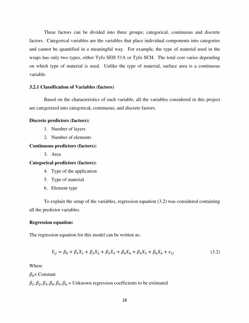
To explain the setup of the variables, regression equation (3.2) was considered containing
all the predictor variables.
Regression equation:
The regression equation for this model can be written as:
��� = �� + ���� + ���� + ���� + ���� + � � + �!�! + "�� (3.2)
Where
��= Constant
��, ��, ��, ��, � , �! = Unknown regression coefficients to be estimated
29
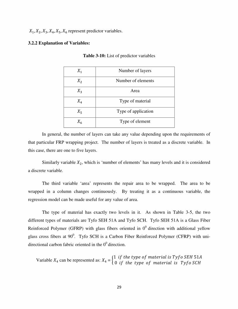
��, ��, ��, ��, � , �! represent predictor variables.
3.2.2 Explanation of Variables:
Table 3-10: List of predictor variables
In general, the number of layers can take any value depending upon the requirements of
that particular FRP wrapping project. The number of layers is treated as a discrete variable. In
this case, there are one to five layers.
Similarly variable ��, which is ‘number of elements’ has many levels and it is considered
a discrete variable.
The third variable ‘area’ represents the repair area to be wrapped. The area to be
wrapped in a column changes continuously. By treating it as a continuous variable, the
regression model can be made useful for any value of area.
The type of material has exactly two levels in it. As shown in Table 3-5, the two
different types of materials are Tyfo SEH 51A and Tyfo SCH. Tyfo SEH 51A is a Glass Fiber
Reinforced Polymer (GFRP) with glass fibers oriented in 00 direction with additional yellow
glass cross fibers at 900. Tyfo SCH is a Carbon Fiber Reinforced Polymer (CFRP) with uni-
directional carbon fabric oriented in the 00 direction.
Variable �� can be represented as: �� = $1 �� �ℎ� �&'� � (���)��� �* +&� ,-. 5100 �� �ℎ� �&'� � (���)��� �* +&� ,1. 2
�� Number of layers
�� Number of elements
�� Area
�� Type of material
� Type of application
�! Type of element
30
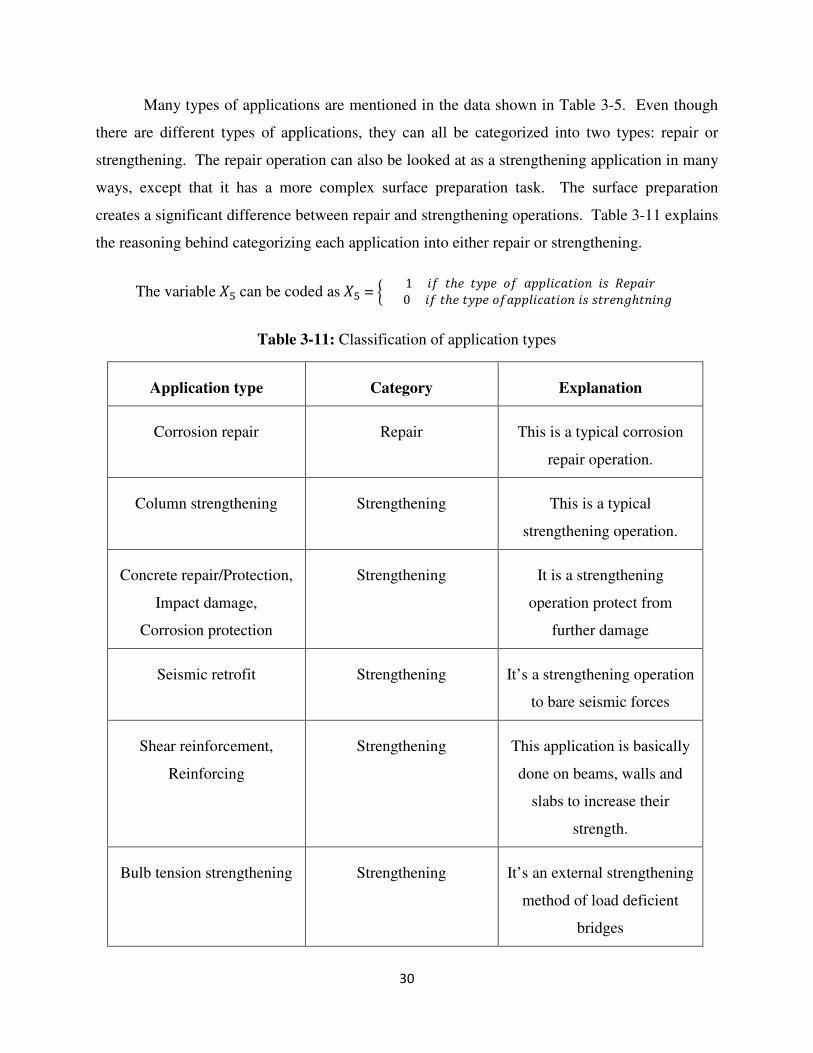
Many types of applications are mentioned in the data shown in Table 3-5. Even though
there are different types of applications, they can all be categorized into two types: repair or
strengthening. The repair operation can also be looked at as a strengthening application in many
ways, except that it has a more complex surface preparation task. The surface preparation
creates a significant difference between repair and strengthening operations. Table 3-11 explains
the reasoning behind categorizing each application into either repair or strengthening.
The variable � can be coded as � = $ 1 �� �ℎ� �&'� � �''��3���� �* �'��) 0 �� �ℎ� �&'� ��''��3���� �* *�)��4ℎ����4 2
Table 3-11: Classification of application types
Application type Category Explanation
Corrosion repair Repair This is a typical corrosion
repair operation.
Column strengthening Strengthening This is a typical
strengthening operation.
Concrete repair/Protection,
Impact damage,
Corrosion protection
Strengthening It is a strengthening
operation protect from
further damage
Seismic retrofit Strengthening It’s a strengthening operation
to bare seismic forces
Shear reinforcement,
Reinforcing
Strengthening This application is basically
done on beams, walls and
slabs to increase their
strength.
Bulb tension strengthening Strengthening It’s an external strengthening
method of load deficient
bridges
31
The variable �! represents the type of element being repaired in the project. There are
four different types of elements, which are columns, bent caps, girders, and piles. There is no
difference between bent caps and girders in terms of the FRP repair procedure. They both come
under the category of beams. That means that there are three categories of elements. Two
variables must be used to represent a categorical variable with three levels. The variables �! and
�5 in Table 3-13 represent the type of element. The value of variable �! is 1 whenever the
element type is column and it is 0 all other times. Similarly the value of variable �5 is 1
whenever the element type is beam and it is 0 all other times.
In addition to the seven variables shown in Table 3-10, another variable is considered to
represent the total area of the wrap, which in turn represents the total material and labor hours it
took for that particular project. Table 3-5 shows that multiple layers of FRP wrap were applied
on some of the elements. To obtain the total wrap area, the area should be multiplied with the
number of layers. Variable �6 represents the total wrap area.
Table 3-12: Values of total wrap area (layers×Area) for FYFE Co.LLC and CFC-WVU projects
Total wrap area (ft2) for FYFE Co.LLC
projects
Total Wrap Area (ft2) for CFC-WVU
projects
7,400 91
42,000 224
5,400 788
4,000 273
23,500 370
19.200 138
1,200 176
1,800 391
6,000 50
12,800 357
5,000 108
32
3.3 The Regression Equation
The regression equation with all the variables can be written as:
��� = �� + ���� + ���� + ���� + ���� + � � + �!�! + �5�5 + �6�6 + "�� (3.4)
Where
�� is the discrete variable representing number of layers
�� is the discrete variable representing number of elements
�� is the continuous variable representing area
�� = $1 �� �ℎ� �&'� � (���)��� �* +&� ,-. 5100 �� �ℎ� �&'� � (���)��� �* +&� ,1. 2
� = $ 1 �� �ℎ� �&'� � �''��3���� �* �'��) 0 �� �ℎ� �&'� ��''��3���� �* *�)��4ℎ����4 2
�! = 71 �� � 3�8(�0 �ℎ�) 9�*� 2
�5 = 7 1 �� � :��(0 �ℎ�) 9�*� 2
�! and �5 are categorical variables representing element type.
�6 is the continuous variable representing total wrap area.
��= Constant
��, ��, ��, ��, � , �!, �5, �6= Unknown regression coefficients to be estimated.
The setup of variables is shown in Table 3-13.
33
Table 3-13: The setup of variables for regression analysis
Number of
layers (X1)
Number of
elements (X2)
Area (ft2)
(X3)
Type of material
(X4)
Application type
(X5)
Element type Number of layers × Area
(X8)
Contract value
Column
(X6)
Beam
(X7)
2 12 3,700 1 1 1 0 7,400 $40,561
4 6 10,500 1 0 1 0 42,000 $118,331
2 26 2,700 1 0 1 0 5,400 $37,934
2 6 2,000 1 0 1 0 4,000 $29,624
5 3 4,700 1 0 1 0 23,500 $160,440
3 38 6,400 0 0 0 1 19,200 $174,887
2 4 600 0 0 0 1 1,200 $32,522
1 5 1,800 0 0 0 1 1,800 $45,958
2 12 3,000 0 0 0 1 6,000 $103,783
4 9 3,200 0 0 0 1 12,800 $136,699
1 50 5,000 0 0 0 1 5,000 $159,134
2 2 46 0 0 0 0 92 $1,100
2 3 112 0 0 0 0 225 $2,698
2 12 394 0 0 0 0 789 $9,479
2 3 137 0 0 0 0 274 $3,292
2 8 185 0 0 0 0 370 $4,447
2 2 69 0 0 0 0 138 $1,659
2 4 88 0 0 0 0 176 $2,119
2 7 196 0 0 0 0 392 $4,704
2 2 25 0 0 0 0 50 $602
2 9 179 0 0 0 0 357 $4,291
2 5 54 0 0 0 0 108 $1,298
These variables are given as inputs in the Minitab software to perform the regression
analysis. The results obtained from Minitab are presented in the next chapter.
34
CHAPTER 4
RESULTS AND DISCUSSION
4.1 Regression Using All Variables
The analysis begins with finding a regression equation that has the best fit and has a
minimum residual. The contract values of columns and girders were analyzed together because
of the similarity in the contract values and the variables to be analyzed. The data on piles is
different to the data on columns and girders both in terms of contract values and the variables.
The values of all the variables and contract values for columns, girders and piles shown in Table
3-13 were inputted in Minitab software and stepwise regression was performed. The results
obtained from the stepwise regression are shown in Figure 4-1.
Figure 4-1: Stepwise regression analysis report on columns and girders
35
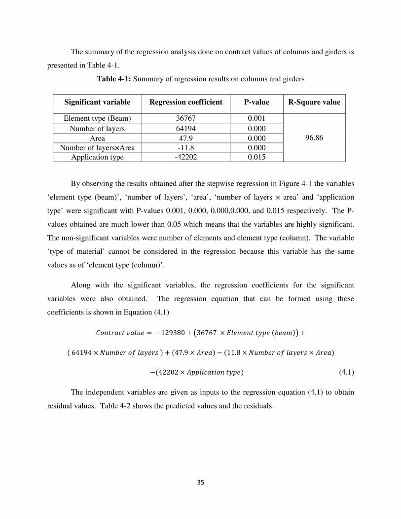
The summary of the regression analysis done on contract values of columns and girders is
presented in Table 4-1.
Table 4-1: Summary of regression results on columns and girders
Significant variable Regression coefficient P-value R-Square value
Element type (Beam) 36767 0.001
96.86 Number of layers 64194 0.000
Area 47.9 0.000
Number of layers×Area -11.8 0.000
Application type -42202 0.015
By observing the results obtained after the stepwise regression in Figure 4-1 the variables
‘element type (beam)’, ‘number of layers’, ‘area’, ‘number of layers × area’ and ‘application
type’ were significant with P-values 0.001, 0.000, 0.000,0.000, and 0.015 respectively. The P-
values obtained are much lower than 0.05 which means that the variables are highly significant.
The non-significant variables were number of elements and element type (column). The variable
‘type of material’ cannot be considered in the regression because this variable has the same
values as of ‘element type (column)’.
Along with the significant variables, the regression coefficients for the significant
variables were also obtained. The regression equation that can be formed using those
coefficients is shown in Equation (4.1)
1��)�3� ;��8� = −129380 + A36767 × -��(��� �&'� D:��(EF +
D 64194 × H8(:�) � ��&�)* E + D47.9 × 0)��E − D11.8 × H8(:�) � ��&�)* × 0)��E
−D42202 × 0''��3���� �&'�E (4.1)
The independent variables are given as inputs to the regression equation (4.1) to obtain
residual values. Table 4-2 shows the predicted values and the residuals.
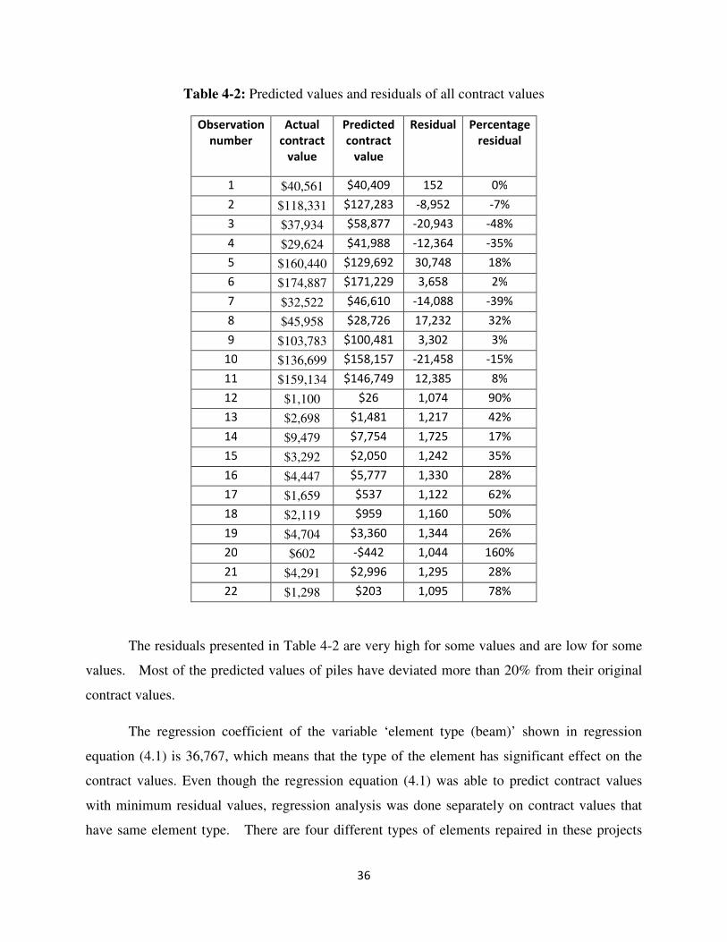
36
Table 4-2: Predicted values and residuals of all contract values
The residuals presented in Table 4-2 are very high for some values and are low for some
values. Most of the predicted values of piles have deviated more than 20% from their original
contract values.
The regression coefficient of the variable ‘element type (beam)’ shown in regression
equation (4.1) is 36,767, which means that the type of the element has significant effect on the
contract values. Even though the regression equation (4.1) was able to predict contract values
with minimum residual values, regression analysis was done separately on contract values that
have same element type. There are four different types of elements repaired in these projects
Observation
number
Actual
contract
value
Predicted
contract
value
Residual Percentage
residual
1 $40,561 $40,409 152 0%
2 $118,331 $127,283 -8,952 -7%
3 $37,934 $58,877 -20,943 -48%
4 $29,624 $41,988 -12,364 -35%
5 $160,440 $129,692 30,748 18%
6 $174,887 $171,229 3,658 2%
7 $32,522 $46,610 -14,088 -39%
8 $45,958 $28,726 17,232 32%
9 $103,783 $100,481 3,302 3%
10 $136,699 $158,157 -21,458 -15%
11 $159,134 $146,749 12,385 8%
12 $1,100 $26 1,074 90%
13 $2,698 $1,481 1,217 42%
14 $9,479 $7,754 1,725 17%
15 $3,292 $2,050 1,242 35%
16 $4,447 $5,777 1,330 28%
17 $1,659 $537 1,122 62%
18 $2,119 $959 1,160 50%
19 $4,704 $3,360 1,344 26%
20 $602 -$442 1,044 160%
21 $4,291 $2,996 1,295 28%
22 $1,298 $203 1,095 78%
37
are: column, bentcap, girder and pile. The element type ‘bentcap’ can be considered as ‘girder’ in
terms of FRP Wrap application procedure. Further analysis on contract values that have same
element type is as follows.
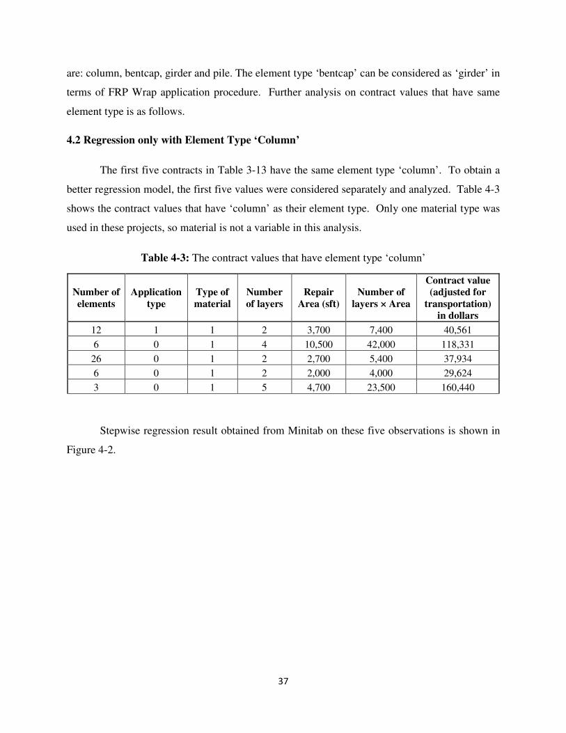
4.2 Regression only with Element Type ‘Column’
The first five contracts in Table 3-13 have the same element type ‘column’. To obtain a
better regression model, the first five values were considered separately and analyzed. Table 4-3
shows the contract values that have ‘column’ as their element type. Only one material type was
used in these projects, so material is not a variable in this analysis.
Table 4-3: The contract values that have element type ‘column’
Number of elements
Application type
Type of material
Number of layers
Repair Area (sft)
Number of layers × Area
Contract value (adjusted for
transportation) in dollars
12 1 1 2 3,700 7,400 40,561
6 0 1 4 10,500 42,000 118,331
26 0 1 2 2,700 5,400 37,934
6 0 1 2 2,000 4,000 29,624
3 0 1 5 4,700 23,500 160,440
Stepwise regression result obtained from Minitab on these five observations is shown in
Figure 4-2.
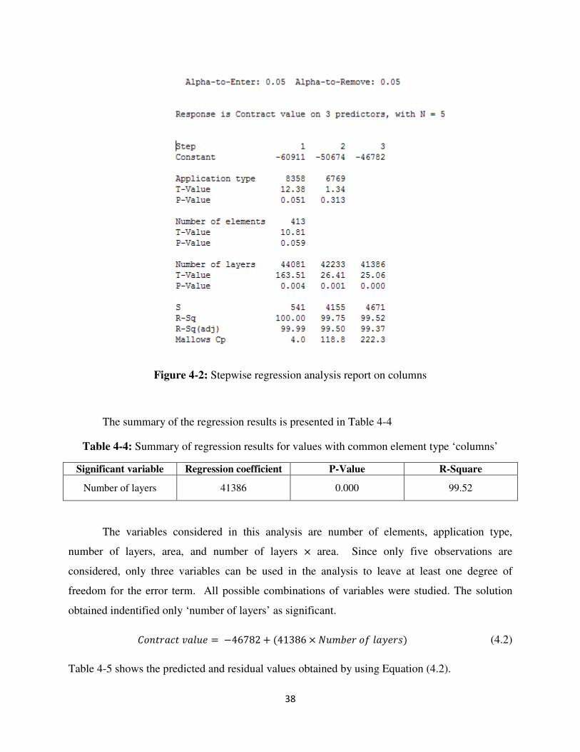
38
Figure 4-2: Stepwise regression analysis report on columns
The summary of the regression results is presented in Table 4-4
Table 4-4: Summary of regression results for values with common element type ‘columns’
Significant variable Regression coefficient P-Value R-Square
Number of layers 41386 0.000 99.52
The variables considered in this analysis are number of elements, application type,
number of layers, area, and number of layers × area. Since only five observations are
considered, only three variables can be used in the analysis to leave at least one degree of
freedom for the error term. All possible combinations of variables were studied. The solution
obtained indentified only ‘number of layers’ as significant.
1��)�3� ;��8� = −46782 + D41386 × H8(:�) � ��&�)*E (4.2)
Table 4-5 shows the predicted and residual values obtained by using Equation (4.2).
39
Table 4-5: Predicted values and residuals (columns)
Actual contract vale
Predicted contract value
Residual % Residual
$40,561 $35,990 4,571 11%
$118,331 $118,762 -431 0%
$37,934 $35,990 1,944 5%
$29,624 $35,990 -6,366 -21%
$160,440 $160,148 292 0%
The residual values obtained by using regression equation 4.2 are smaller for contract
values 3, 4, and 5.
The 95% confidence interval band for contract value obtained using the regression
equation (4.2) is shown in Figure 4-3. The band varies by approximately ±9000 over the range
of the data that is for two to five layers. The 95% confidence intervals for the predicted values
were calculated using equation (4.4) and are presented in Table 4-6.
&JK ± �M �⁄ ,O��PQ�R S�O + DTU�TVEW
∑ DTU�TVEWYUZ[\ (4.4)
Where
&JK is the predicted value
]� is the variable at which the observation was made
n is the number of observations
Table 4-6: 95% Confidence intervals for contract values on columns
Number of layers 95% confidence interval for
contract value 2 ±8,474
3 ±6,648
4 ±8,474
5 ±12,436
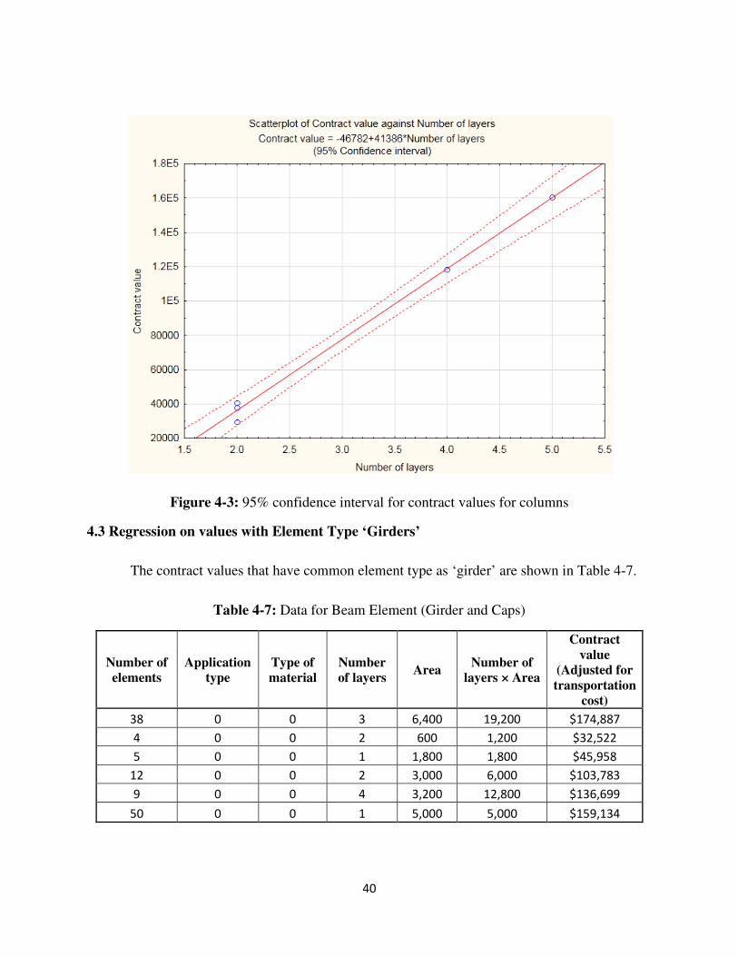
40
Figure 4-3: 95% confidence interval for contract values for columns
4.3 Regression on values with Element Type ‘Girders’
The contract values that have common element type as ‘girder’ are shown in Table 4-7.
Table 4-7: Data for Beam Element (Girder and Caps)
Number of elements
Application type
Type of material
Number of layers
Area Number of
layers × Area
Contract value
(Adjusted for transportation
cost)
38 0 0 3 6,400 19,200 $174,887
4 0 0 2 600 1,200 $32,522
5 0 0 1 1,800 1,800 $45,958
12 0 0 2 3,000 6,000 $103,783
9 0 0 4 3,200 12,800 $136,699
50 0 0 1 5,000 5,000 $159,134
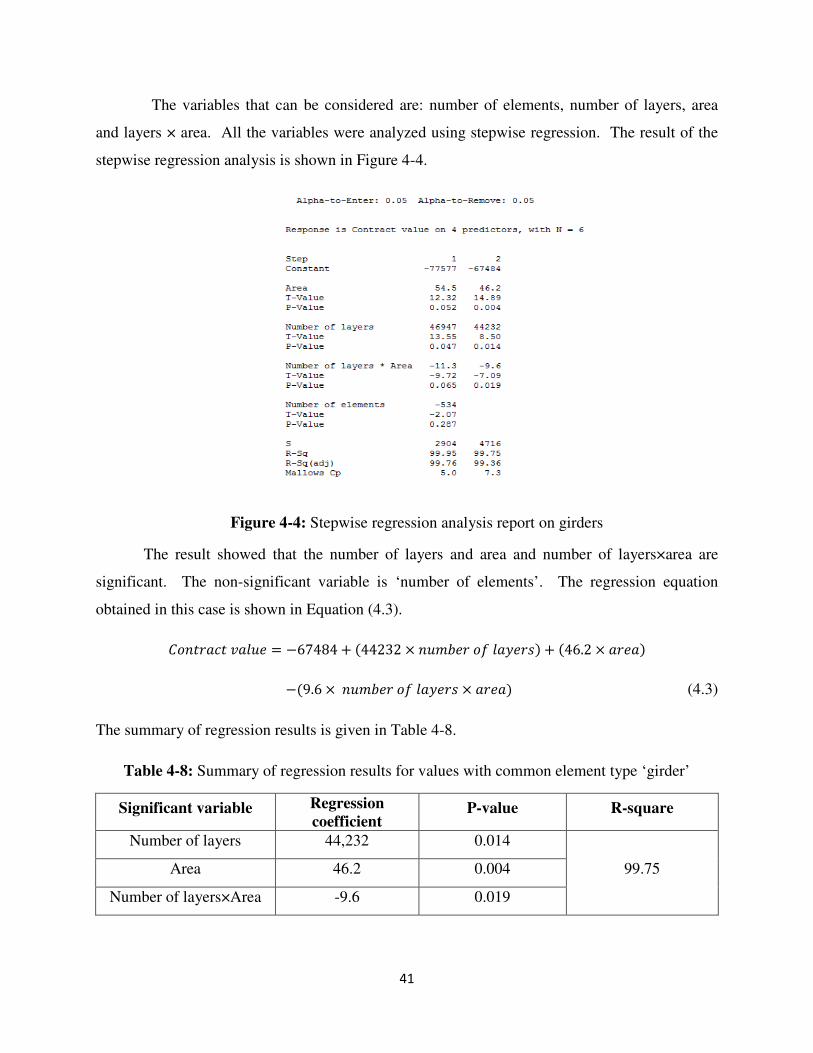
41
The variables that can be considered are: number of elements, number of layers, area
and layers × area. All the variables were analyzed using stepwise regression. The result of the
stepwise regression analysis is shown in Figure 4-4.
Figure 4-4: Stepwise regression analysis report on girders The result showed that the number of layers and area and number of layers×area are
significant. The non-significant variable is ‘number of elements’. The regression equation
obtained in this case is shown in Equation (4.3).
1��)�3� ;��8� = −67484 + D44232 × �8(:�) � ��&�)*E + D46.2 × �)��E
−D9.6 × �8(:�) � ��&�)* × �)��E (4.3)
The summary of regression results is given in Table 4-8.
Table 4-8: Summary of regression results for values with common element type ‘girder’
Significant variable Regression coefficient
P-value R-square
Number of layers 44,232 0.014
99.75 Area 46.2 0.004
Number of layers×Area -9.6 0.019
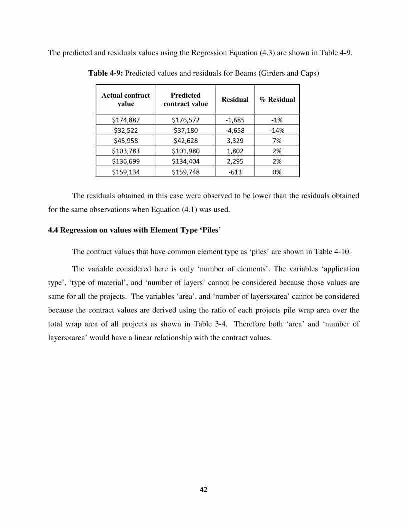
42
The predicted and residuals values using the Regression Equation (4.3) are shown in Table 4-9.
Table 4-9: Predicted values and residuals for Beams (Girders and Caps) Actual contract
value Predicted
contract value Residual % Residual
$174,887 $176,572 -1,685 -1%
$32,522 $37,180 -4,658 -14%
$45,958 $42,628 3,329 7%
$103,783 $101,980 1,802 2%
$136,699 $134,404 2,295 2%
$159,134 $159,748 -613 0%
The residuals obtained in this case were observed to be lower than the residuals obtained
for the same observations when Equation (4.1) was used.
4.4 Regression on values with Element Type ‘Piles’
The contract values that have common element type as ‘piles’ are shown in Table 4-10.
The variable considered here is only ‘number of elements’. The variables ‘application
type’, ‘type of material’, and ‘number of layers’ cannot be considered because those values are
same for all the projects. The variables ‘area’, and ‘number of layers×area’ cannot be considered
because the contract values are derived using the ratio of each projects pile wrap area over the
total wrap area of all projects as shown in Table 3-4. Therefore both ‘area’ and ‘number of
layers×area’ would have a linear relationship with the contract values.
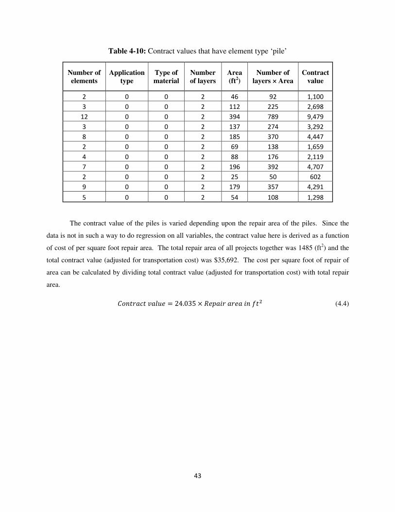
43
Table 4-10: Contract values that have element type ‘pile’
Number of elements
Application type
Type of material
Number of layers
Area (ft2)
Number of layers × Area
Contract value
2 0 0 2 46 92 1,100
3 0 0 2 112 225 2,698
12 0 0 2 394 789 9,479
3 0 0 2 137 274 3,292
8 0 0 2 185 370 4,447
2 0 0 2 69 138 1,659
4 0 0 2 88 176 2,119
7 0 0 2 196 392 4,707
2 0 0 2 25 50 602
9 0 0 2 179 357 4,291
5 0 0 2 54 108 1,298
The contract value of the piles is varied depending upon the repair area of the piles. Since the
data is not in such a way to do regression on all variables, the contract value here is derived as a function
of cost of per square foot repair area. The total repair area of all projects together was 1485 (ft2) and the
total contract value (adjusted for transportation cost) was $35,692. The cost per square foot of repair of
area can be calculated by dividing total contract value (adjusted for transportation cost) with total repair
area.
1��)�3� ;��8� = 24.035 × �'��) �)�� �� ��� (4.4)
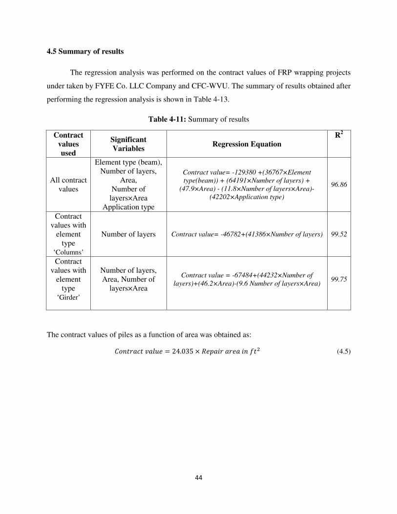
44
4.5 Summary of results
The regression analysis was performed on the contract values of FRP wrapping projects
under taken by FYFE Co. LLC Company and CFC-WVU. The summary of results obtained after
performing the regression analysis is shown in Table 4-13.
Table 4-11: Summary of results Contract
values used
Significant Variables
Regression Equation R2
All contract values
Element type (beam), Number of layers,
Area, Number of
layers×Area Application type
Contract value= -129380 +(36767×Element
type(beam)) + (64191×Number of layers) +
(47.9×Area) - (11.8×Number of layers×Area)-
(42202×Application type)
96.86
Contract values with
element type
‘Columns’
Number of layers Contract value= -46782+(41386×Number of layers) 99.52
Contract values with
element type
‘Girder’
Number of layers, Area, Number of
layers×Area
Contract value = -67484+(44232×Number of
layers)+(46.2×Area)-(9.6 Number of layers×Area) 99.75
The contract values of piles as a function of area was obtained as:
1��)�3� ;��8� = 24.035 × �'��) �)�� �� ��� (4.5)
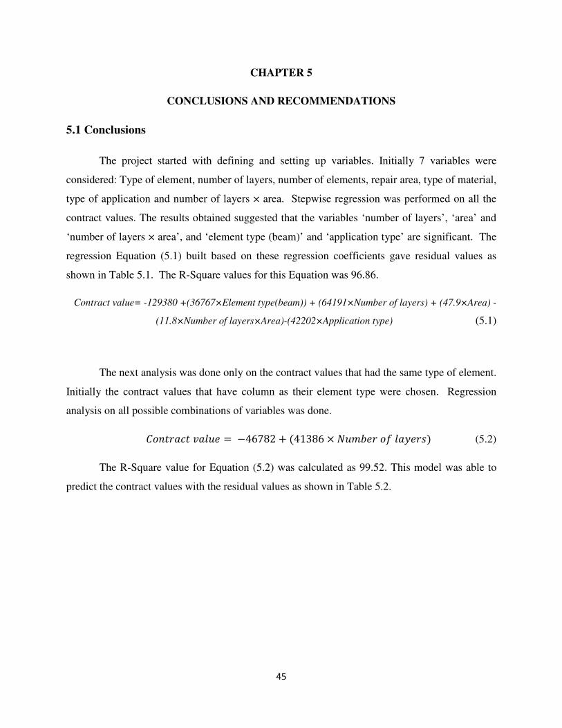
45
CHAPTER 5
CONCLUSIONS AND RECOMMENDATIONS
5.1 Conclusions
The project started with defining and setting up variables. Initially 7 variables were
considered: Type of element, number of layers, number of elements, repair area, type of material,
type of application and number of layers × area. Stepwise regression was performed on all the
contract values. The results obtained suggested that the variables ‘number of layers’, ‘area’ and
‘number of layers × area’, and ‘element type (beam)’ and ‘application type’ are significant. The
regression Equation (5.1) built based on these regression coefficients gave residual values as
shown in Table 5.1. The R-Square values for this Equation was 96.86.
Contract value= -129380 +(36767×Element type(beam)) + (64191×Number of layers) + (47.9×Area) -
(11.8×Number of layers×Area)-(42202×Application type) (5.1)
The next analysis was done only on the contract values that had the same type of element.
Initially the contract values that have column as their element type were chosen. Regression
analysis on all possible combinations of variables was done.
1��)�3� ;��8� = −46782 + D41386 × H8(:�) � ��&�)*E (5.2)
The R-Square value for Equation (5.2) was calculated as 99.52. This model was able to
predict the contract values with the residual values as shown in Table 5.2.
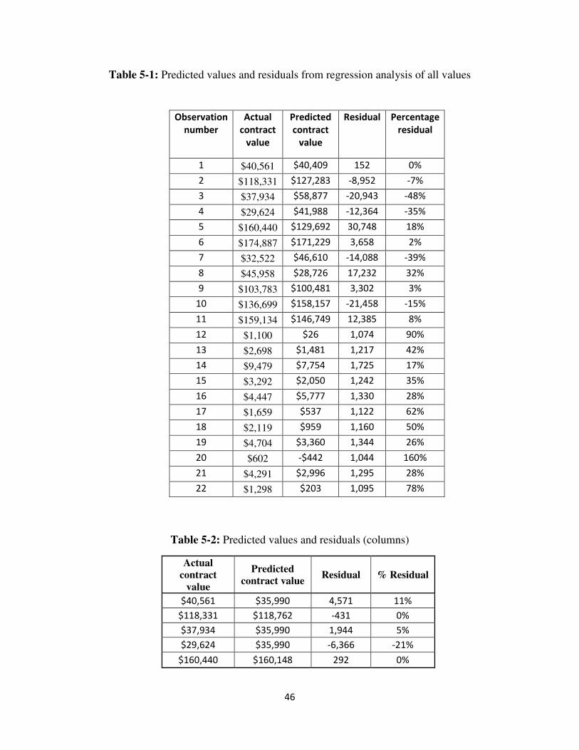
46
Table 5-1: Predicted values and residuals from regression analysis of all values
Table 5-2: Predicted values and residuals (columns)
Actual contract
value
Predicted contract value
Residual % Residual
$40,561 $35,990 4,571 11%
$118,331 $118,762 -431 0%
$37,934 $35,990 1,944 5%
$29,624 $35,990 -6,366 -21%
$160,440 $160,148 292 0%
Observation
number
Actual
contract
value
Predicted
contract
value
Residual Percentage
residual
1 $40,561 $40,409 152 0%
2 $118,331 $127,283 -8,952 -7%
3 $37,934 $58,877 -20,943 -48%
4 $29,624 $41,988 -12,364 -35%
5 $160,440 $129,692 30,748 18%
6 $174,887 $171,229 3,658 2%
7 $32,522 $46,610 -14,088 -39%
8 $45,958 $28,726 17,232 32%
9 $103,783 $100,481 3,302 3%
10 $136,699 $158,157 -21,458 -15%
11 $159,134 $146,749 12,385 8%
12 $1,100 $26 1,074 90%
13 $2,698 $1,481 1,217 42%
14 $9,479 $7,754 1,725 17%
15 $3,292 $2,050 1,242 35%
16 $4,447 $5,777 1,330 28%
17 $1,659 $537 1,122 62%
18 $2,119 $959 1,160 50%
19 $4,704 $3,360 1,344 26%
20 $602 -$442 1,044 160%
21 $4,291 $2,996 1,295 28%
22 $1,298 $203 1,095 78%
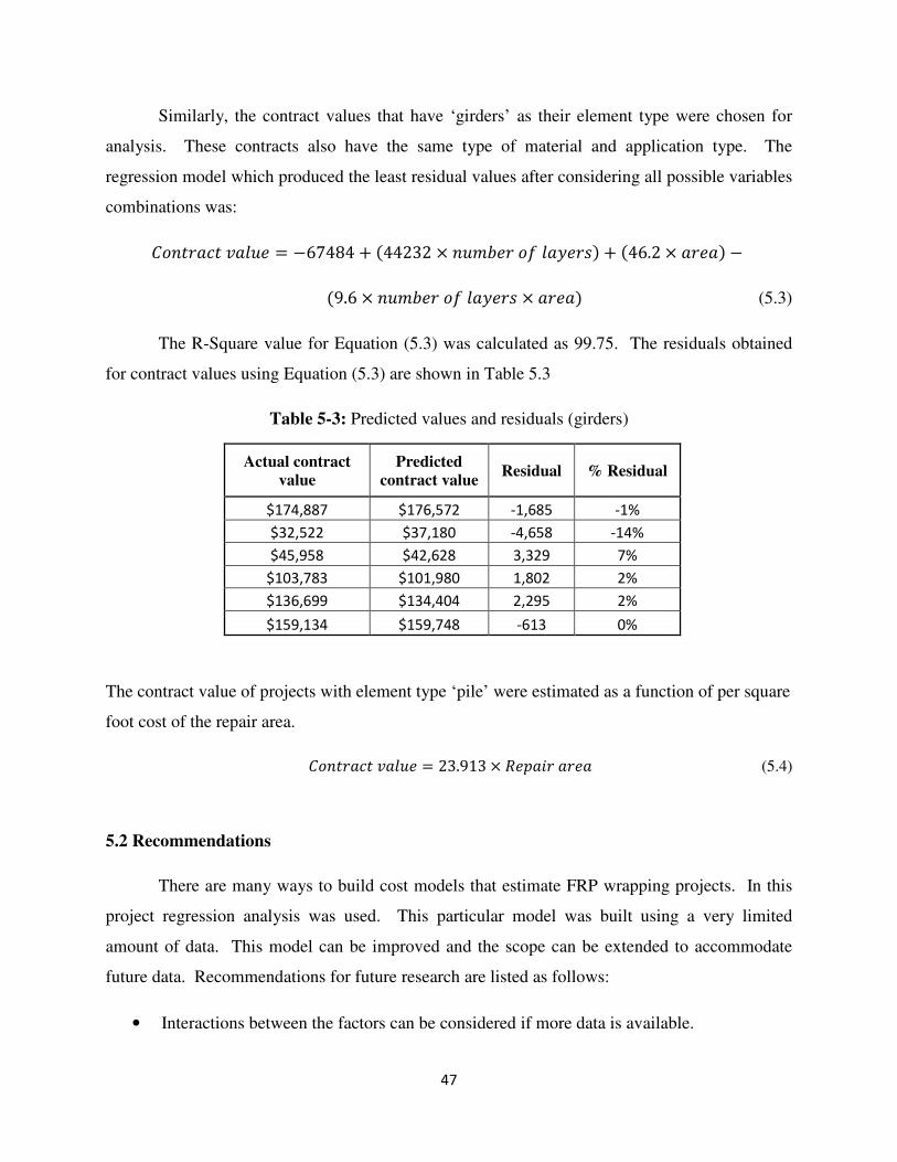
47
Similarly, the contract values that have ‘girders’ as their element type were chosen for
analysis. These contracts also have the same type of material and application type. The
regression model which produced the least residual values after considering all possible variables
combinations was:
1��)�3� ;��8� = −67484 + D44232 × �8(:�) � ��&�)*E + D46.2 × �)��E − D9.6 × �8(:�) � ��&�)* × �)��E (5.3)
The R-Square value for Equation (5.3) was calculated as 99.75. The residuals obtained
for contract values using Equation (5.3) are shown in Table 5.3
Table 5-3: Predicted values and residuals (girders)
Actual contract value
Predicted contract value
Residual % Residual
$174,887 $176,572 -1,685 -1%
$32,522 $37,180 -4,658 -14%
$45,958 $42,628 3,329 7%
$103,783 $101,980 1,802 2%
$136,699 $134,404 2,295 2%
$159,134 $159,748 -613 0%
The contract value of projects with element type ‘pile’ were estimated as a function of per square
foot cost of the repair area.
1��)�3� ;��8� = 23.913 × �'��) �)�� (5.4)
5.2 Recommendations
There are many ways to build cost models that estimate FRP wrapping projects. In this
project regression analysis was used. This particular model was built using a very limited
amount of data. This model can be improved and the scope can be extended to accommodate
future data. Recommendations for future research are listed as follows:
• Interactions between the factors can be considered if more data is available.
48
• The percentage residual (error) can be reduced by fitting a better regression equation
• Design of experiments procedures can be used to identify the significant variables and
interactions if more data is available.
• The bottom-up approach could be considered if more detailed cost data is available in the
future. The contract values can be broken down into their basic cost elements and then a
bottom-up approach can be used. A data sheet, shown in Appendix A, was prepared to
break the total contract values in to basic parameters thought to be useful for estimating.
The data sheet was sent to a contractor, but the results have not been received. Once it
becomes available a more accurate model can be built using a bottom up approach.

49
APPENDIX A
DATA SHEET
Column Description (Length, width, radius etc.): _____________________
_____________________
Tasks Costs
Man-hours Materials cost
(Materials/ quantities) Equipment rental (Equipment type)
Removal of loose/spalling concrete (air chiseling)
Cleaning of surface(sand blasting )
Dust and debris removal (compressed air)
Strands cleaning (using acetone)
Application of corrosion inhibitor/epoxy cement
Reformation of cross section
Rounding of corners
Resin injection/Putty (To fill the cracks)
Other operations
Total ___________ ________________ _______________

50
Data sheet (Continued)
FRP application
Tasks Cost
Material (Type/Quantity)
Man-hours Equipment
Resin application
FRP application
Painting/End sealing applied
Other
Total ______________ ______________ ______________
Non-Destructive Testing (NDT)
Task Cost
Man-hours Equipment (Type/Rental) Testing
Total ____________ ______________
Location of the Project: ________________
Transportation costs: ___________________
Overhead costs: ______________________
Profit percentage: ____________________
* If you cannot provide the profit percentage, please try to include them in the overhead costs.
Thank you.
51
REFERENCES
keepwvmoving. (2010, 02 23). Retrieved January 20, 2011, from West Virginians for better
transportation:
http://www.keepwvmoving.org/news/news/Average-Annual-Cost-To-Motorists-Is-280--Harsh-
2010-Winter-Weather-Having-Widespread-Negative-Impacts-On-Roads-Bridges,441.aspx
WV DOT. (2010, December). Retrieved January 25, 2011, from STIP:
http://gis.wvdot.com/gti/FedStip/Stip_Narrative.pdf
Brown. (2005). Infrared thermography inspection of Fiber Reinforced Polymers bonded to
concrete. Gainesville: University of Florida.
Shoemaker C. L. (2001). Effect of Wrapping Chloride Contaminated Structural Concrete with
Multiple Layers of Glass Fiber/Composites and Resin. Austin: University of Texas.
Chhabra, Y. (2011). Bridge Rehabilitation Techniques. Retrieved January 27, 2011, from
dsbrwon: http://www.dsbrown.com/Resources/Articles/Masterbuilder.pdf
Clarke, J. (1998, February). Materials World, pp. 78-80.
Clyne, H. (1996). An Introduction to Composite Materials. Cambridge University Press.
corecomposites.com. (2005).
http://www.corecomposites.com/media/aboutCarbon.pdf. Retrieved February 26, 2011, from
www.corecomposite.com: http://www.corecomposites.com/media/aboutCarbon.pdf
David Hartman, Mark E. Greenwood, David M.Miller (1996).
http://www.agy.com/technical_info/graphics_PDFs/HighStrengthTechPaperEng.pdf. Retrieved
February 26, 2011, from www.agy.com:
http://www.agy.com/technical_info/graphics_PDFs/HighStrengthTechPaperEng.pdf
Halvard E. Nystrom, Steve E. Watkins, Antonio Nanni, Susan Murray (2003). Financial
Viability of Fiber-Reinforced Polymer Bridges. Journal of Management in Engineering, pp.2-8
Homam, S. (2000). Durability of Fiber Reinforced Polymers and External FRP-Concrete bond.
Department of Civil Engineering . Toronto: University of Toronto.
Lopez-Anido, R (2002). Repair of Wood Piles with Reinforced Composites. University of Maine,
Advanced Engineering Wood Composites Center, Orono.
Lopez-Anido, R. (2001). Life Cycle Cost Evaluation of FRP Composite Bridge
Decks.Transportation Research Board. Washington D.C 80th annual meeting.pp 2-16
Vijay P.V, Gangarao H.V.S, Ruifeng Liang, Mark Skidmore. (2011). Rapid Restoration of
Timber Railroad Bridges. ANTEC.
52
Rajan Sen, G. M. (2006). Application of FRP Composites for Underwater Piles Repair.
ScienceDirect, 2-8.
Roychoudhury, P. (2001). A Life Cycle Cost Estimation Model For FRP Bridge Decks.
Morgantown: West Virginia University, PP 4-10
Sidharta Sahirman (2009). Estimating Life-cycle Cost of West Virginia Fiber Reinforced
Polymer (FRP) Bridge Decks. Morgantown: West Virginia University, pp 125-127.
Wilde, D. (1988). Proceedings of the International Conference on Computer Aided Design in
Composite Material Technology. Computational Mechanics Publication. Springer.PP 6-9
Worth, F. (2005). Analisis of Aquawrap for Use in Repairing Damaged Pipelines. Azusa: Air
Logistics Corporation.PP 1-9


![JPDUDVOLV#LVPHQJHQKDULD FRP EU LJRUSXII#JPDLO FRP€¦ · hjdyd#lvphqjhqkduld frp eu hysurmhwrv hqj#jpdlo frp hgx ]lool#krwpdlo frp ilolsh#edvhdpelhqwdo frp eu jerued#fdvdq frp eu](https://img.pdfslide.net/doc/110x75/5fa5bbc4c11b4c37f05fd0f4/jpdudvolvlvphqjhqkduld-frp-eu-ljrusxiijpdlo-hjdydlvphqjhqkduld-frp-eu-hysurmhwrv.jpg)