Cost evaluation and life cycle assessmentof biogas upgrading technologies for ananaerobic digestion case study in theUnited States

Marina Jennifer Hauser

Master in Industrial Ecology

Supervisor: Helge Brattebø, EPT

Department of Energy and Process Engineering

Submission date: June 2017

Norwegian University of Science and Technology

Marina Jennifer Hauser

Cost evaluation and life cycle assessment of biogas

upgrading technologies for an anaerobic digestion

case study in the United States

Trondheim, 06 2017

Thes

is

NT

NU

No

rweg

ian U

niv

ersi

ty o

f

Sci

ence

and

Tec

hno

log

y

Fac

ult

y o

f E

ngin

eeri

ng S

cien

ce

and

Tec

hno

log

y

Dep

artm

ent

of

Ener

gy a

nd

Pro

cess

En

gin

eeri

ng

i

Preface

This thesis is carried out as the final assignment for the Nordic Five Tech master program in

Residual Resources Engineering at the Norwegian University of Science and Technology (NTNU)

in Trondheim in collaboration with the Danish Technical University (DTU) in Copenhagen and

the company B&W Megtec from De Pere, Wi. The presented study counts for 30 ECTS and has

been written at the Department of Energy and Process Engineering at NTNU in the period from

January 2017 to June 2017. The thesis builds on the project work carried out in the Fall semester

2016 at NTNU called “Energy evaluation of biogas upgrading technologies for an anaerobic

digestion case study in the United States”.

From the project work done in the previous semester, knowledge regarding the anaerobic digestion

and the different biogas upgrading technologies was already available. Besides, also most data

needed for the life cycle assessment and cost evaluation was also already found in literature as no

plant specific data was available from the company. Due to time and data restrictions, it was only

possible to analyze a system for anaerobic digestion using mixed waste in the life cycle assessment

but not one for using wastewater sludge. For the cost evaluation, data was only available for plants

with gas flow ranges up to 2000 Nm3/h and not 15,000 Nm3/h as specified in the assignment text.

Therefore, these two points of the assignment text could not be evaluated.

First, I would like to thank Gerald Norz not only for providing me with a topic for this thesis and

letting me work with such a renowned company as B&W Megtec, but also for helping me

throughout the project with advice and inputs, and for giving me a tour of the company and

showing me around the office in De Pere. Then I would also like to thank Helge Brattebø for being

my supervisor and for guiding me through this project. I would also like to thank Marina Zabrodina

for giving me very detailed feedback on drafts of this thesis. Lastly, I would like to thank Anders

Damgaard for helping me with any problems or questions I had regarding the modelling and the

EASETECH software.

Trondheim, June 12th 2017

________________________

Marina Hauser

ii

Abstract

Globally, around one third of the food produced is lost or wasted. Instead of landfilling or

incinerating, organic municipal solid waste has increasingly been used in anaerobic digestion in

order to produce biogas. The produced biogas contains around 60-70% methane, 30-40% carbon

dioxide, and minor parts of impurities such as hydrogen sulfide, nitrogen, or water vapor. The

biogas can be cleaned of impurities and upgraded by removing the carbon dioxide to substitute

either natural gas in the national gas grid or liquid natural gas for vehicles. Different technologies

exist for the removal of the carbon dioxide. The most widely used technologies are pressure swing

adsorption, water scrubbing, amine scrubbing, membrane separation, and cryogenic separation.

These five technologies were assessed in this study using literature data.

The first purpose of this study is to evaluate the environmental impact of the anaerobic digestion

with following biogas upgrading in the geographical context of the United States. A life cycle

assessment considering all the impacts from the anaerobic digestion to the substitution of natural

gas including the biogas upgrading technology, gas compression and possible leakages along the

way was performed using the EASETECH software. The normalized results show that the largest

impacts occur in Freshwater Eutrophication and Global Warming. The largest savings are achieved

in Freshwater Ecotoxicity, followed by Marine Ecotoxicity, fossil Depletion and Human Toxicity.

Of the total 14 impact categories, cryogenic separation had the largest saving in eight impact

categories and the largest impact in only one. However, including the sensitivity analysis, it was

found that the uncertainty is so large that the error bars overlap for most impact categories and it

is therefore most of the time not possible to show clearly which category is best or worst. Only for

climate change, cryogenic separation clearly had the smallest impact, and for human toxicity and

marine ecotoxicity, cryogenic separation clearly had the largest saving. It was also found that for

the two impact categories with the largest environmental impact, the biogas production of the

anaerobic digestion was the major contributing process for three of the scenarios. For the four

impact categories with a negative impact, the substitution of natural gas was the major contributor.

This study also evaluates the costs and revenues associated with the anaerobic digestion and the

following biogas upgrading. The calculations included investment cost, yearly costs, as well as

income from tipping fees, the sale of biogas, and the sale of digestate. The net present value was

calculated for plants with three raw biogas flow rates to compare the profitability of anaerobic

digestion with following pressure swing adsorption, water scrubbing, and amine scrubbing. The

analysis showed that water scrubbing and amine scrubbing had similar net present values, whereas

the net present values for pressure swing adsorption was considerably lower. The sensitivity

analysis showed that the factors with the largest sensitivity are the tipping fee and the biogas yield

of the food waste which are both part of the anaerobic digestion. However, there is large

uncertainty in the data used. Only one set of data was available from literature. Also, this data is

from Europe and from 2008 adding additional uncertainty.

The conclusion was that depending on the goal of a project, such as low environmental impact,

high energy efficiency, low methane slip, etc., a different technology may be preferred. Also, in

order to get a complete picture, data from real plants need to be available.

iii

Terminology

AD Anaerobic Digester

AS Amine Scrubbing

CBG Compressed Biogas

CH4 Methane

CNG Compressed Natural Gas

CO2 Carbon Dioxide

C/N carbon/nitrogen

DMEA Dimethylethanol amine

EPA Environmental Protection Agency

GHG Greenhouse Gas

GWP Global Warming Potential

H2S Hydrogen Sulfide

ISO International Standards Organization

LBG Liquefied Biogas

LCA Life Cycle Assessment

LCI Life Cycle Inventory

LCIA Life Cycle Impact Assessment

LHV Lower Heating Value

LNG Liquid Natural Gas

MEA Monoethanol Amine

MPa Megapascal (1 MPa = 0.1 bar)

MSW Municipal Solid Waste

NPV Net Present Value

N2 Nitrogen

OMSW Organic Municipal Solid Waste

O2 Oxygen

PSA Pressure Swing Adsorption

iv

RFS Renewable Fuel Standard

TS Total Solids

VFA Volatile Fatty Acids

VS Volatile Solids

WS Water Scrubbing

WW Wet Weight

v

Table of Contents

1. Introduction .......................................................................................................................................... 1

1.1. Background ................................................................................................................................... 1

1.2. Research Question ........................................................................................................................ 3

1.3. Structure of the Thesis .................................................................................................................. 4

2. Literature & Theory ............................................................................................................................... 5

2.1. Biogas Systems from Waste .......................................................................................................... 5

2.2. Biogas Upgrading Technologies .................................................................................................... 7

2.2.1. Removal of Impurities ........................................................................................................... 8

2.2.2. Pressure Swing Adsorption ................................................................................................. 10

2.2.3. Water Scrubbing ................................................................................................................. 11

2.2.4. Amine Scrubbing ................................................................................................................. 13

2.2.5. Membrane Separation ........................................................................................................ 14

2.2.6. Cryogenic Separation .......................................................................................................... 16

3. Methods .............................................................................................................................................. 17

3.1. Case Study Description ............................................................................................................... 17

3.2. Life Cycle Assessment ................................................................................................................. 17

3.2.1. Methodology ....................................................................................................................... 17

3.2.2. The Model ........................................................................................................................... 22

3.2.3. Data Collection .................................................................................................................... 24

3.2.3.1. Anaerobic Digestion ........................................................................................................ 24

3.2.3.2. Pressure Swing Adsorption ............................................................................................. 27

3.2.3.3. Water Scrubbing ............................................................................................................. 29

3.2.3.4. Amine Scrubbing ............................................................................................................. 31

3.2.3.5. Membrane Separation .................................................................................................... 33

3.2.3.6. Cryogenic Separation ...................................................................................................... 34

3.3. Cost Evaluation ........................................................................................................................... 35

3.3.1. Methodology ....................................................................................................................... 35

3.3.2. The Model ........................................................................................................................... 36

3.3.3. Data Collection .................................................................................................................... 38

3.3.3.1. Anaerobic Digestion ........................................................................................................ 38

3.3.3.2. Pressure Swing Adsorption ............................................................................................. 40

vi

3.3.3.3. Water Scrubbing ............................................................................................................. 42

3.3.3.4. Amine Scrubbing ............................................................................................................. 43

4. Results ................................................................................................................................................. 45

4.1. Life Cycle Assessment ................................................................................................................. 45

4.1.1. Perturbation Analysis .......................................................................................................... 54

4.1.2. Uncertainty Propagation ..................................................................................................... 57

4.2. Cost Evaluation ........................................................................................................................... 63

4.2.1. Sensitivity Analysis .............................................................................................................. 65

5. Discussion ............................................................................................................................................ 68

5.1. Life Cycle Assessment ................................................................................................................. 68

5.1.1. Main Findings ...................................................................................................................... 68

5.1.2. Agreement with Literature ................................................................................................. 69

5.1.3. Strength and Weaknesses ................................................................................................... 70

5.2. Cost Evaluation ........................................................................................................................... 71

5.2.1. Main Findings ...................................................................................................................... 71

5.2.2. Agreement with Literature ................................................................................................. 74

5.2.3. Strength and Weaknesses ................................................................................................... 76

5.3. Implication of the Findings.......................................................................................................... 77

6. Conclusions ......................................................................................................................................... 80

7. List of References ................................................................................................................................ 82

Appendix I: Master Thesis Assignment Text ............................................................................................... 86

Appendix II: CO2 Transfer in Biogas Upgrading ........................................................................................... 89

Appendix III: List of Geographies from Ecoinvent ....................................................................................... 91

Appendix IV: EASETECH Screenshots .......................................................................................................... 92

Appendix V: Sensitivity Ratio Calculations for LCA ..................................................................................... 95

Appendix VI: Normalized Sensitivity Ratios for P2 ...................................................................................... 98

Appendix VII: Results from NPV calculations .............................................................................................. 99

vii

List of Figures Titelpage: Anaerobic Digester in Hashøj, DK (Hashøj Biogas, 2017) ......................................................... 0

Figure 1: Volume Target for Renewable Fuel (US EPA, 2016) ................................................................... 2

Figure 2: Chemical Reactions during Anaerobic Digestion (Costa et al., 2015) .......................................... 6

Figure 3: Application of upgrading technology in Europe (Biogaspartner, 2011) ....................................... 8

Figure 4: Process Flow Diagram of Pressure Swing Adsorption (Ryckebosch et al., 2011) ...................... 10

Figure 5: Process Flow Diagram of Water Scrubbing (Bauer et al., 2013) ................................................ 12

Figure 6: Process Flow Diagram of an Amine Scrubber (Bauer et al., 2013) ............................................ 14

Figure 7: Process Flow Diagram of Membrane Separation (Bauer et al., 2013) ........................................ 15

Figure 8: Process Flow Diagram of Cryogenic Separation (Yang et al., 2014) .......................................... 16

Figure 9: The Subsystems evaluated in this Case Study ............................................................................. 17

Figure 10: Boundaries of LCI of Products vs LCI of Solid Waste (M. Z. Hauschild & Barlaz, 2011) ...... 18

Figure 11: Framework for Life Cycle Assessment (JRC European Commission, 2010) ........................... 19

Figure 12: Midpoints and Endpoints and their Connections (M. Hauschild, 2015b) ................................. 21

Figure 13: Iterative Approach of a Life Cycle Analysis (M. Hauschild, 2015a) ........................................ 22

Figure 14: Model for Life Cycle Assessment ............................................................................................. 23

Figure 15: Anaerobic Digestion Model for Cost Evaluation ...................................................................... 37

Figure 16: Biogas Upgrading Model for Cost Evaluation .......................................................................... 37

Figure 17: Characterized Results from EASETECH (ReCiPe Hierarchist World) .................................... 45

Figure 18: Internally Normalized Results from EASETECH ..................................................................... 46

Figure 19: Externally Normalized Results from EASETECH (ReCiPe Hierarchist World) ...................... 46

Figure 20: Contribution Analysis for Climate Change ............................................................................... 48

Figure 21: Contribution Analysis for Freshwater Eutrophication ............................................................... 49

Figure 22: Contribution Analysis for Human Toxicity ............................................................................... 50

Figure 23: Contribution Analysis for Freshwater Ecotoxicity .................................................................... 51

Figure 24: Contribution Analysis for Marine Ecotoxicity .......................................................................... 52

Figure 25:Contribution Analysis for Fossil Depletion ................................................................................ 53

Figure 26: Uncertainty Analysis for Climate Change ................................................................................. 59

Figure 27: Uncertainty Analysis for Freshwater Eutrophication ................................................................ 60

Figure 28: Uncertainty Analysis for Human Toxicity ................................................................................ 60

Figure 29: Uncertainty Analysis for Freshwater Ecotoxicity ..................................................................... 61

Figure 30: Uncertainty Analysis for Marine Ecotoxicity ............................................................................ 62

Figure 31: Uncertainty Analysis for Fossil Depletion ................................................................................ 62

Figure 32: Net Present Values for Anaerobic Digestion ............................................................................. 63

Figure 33: Net Present Values per Raw Biogas Flow Rate for Anaerobic Digestion ................................. 64

Figure 34: Net Present Values for Biogas Upgrading Technologies .......................................................... 64

Figure 35: Net Present Values for Anaerobic Digestion and Biogas Upgrading Technologies ................. 65

Figure 36:Normalized Impact Scores for the Six Largest Categories with Uncertainty Bars .................... 68

Figure 37: Global Warming Potential from Starr et al. (2014) ................................................................... 70

Figure 38: Comparison of Investment Cost from Bauer et al. (2013) & Urban (2008) .............................. 75

Figure 39: Net Present Values for PSA, WS, and AS using 2008 and 2017 Exchange Rates .................... 77

Figure 40: Flowchart of Methane and Carbon Dioxide during Anaerobic Digestion ................................. 89

viii

List of Tables Table 1: Composition of Biogas, Landfill Gas and Natural Gas (Petersson & Wellinger, 2009) ................ 7

Table 2: Material Fractions used for “Disposed Household Organic Waste” in EASETECH ................... 25

Table 3: Transfer of material fractions from organic waste to feedstock (Naroznova et al., 2016) ........... 25

Table 4: External Processes used for “Biogas Production, Thermophilic” ................................................. 27

Table 5: External Processes used for “PSA” .............................................................................................. 28

Table 6: External Processes used for “Water Scrubbing” ........................................................................... 30

Table 7: External Processes used for "Waste Water Treatment" ................................................................ 31

Table 8: External Processes used for “Amine Scrubbing”.......................................................................... 32

Table 9: External Processes used for “Membrane Separation” .................................................................. 33

Table 10: External Processes used for “Cryogenic Separation” ................................................................. 34

Table 11: Initial Investment Cost ($) for AD converted to US Dollars and adjusted for Inflation ............. 38

Table 12: Yearly Costs ($/yr) for AD converted to US Dollars and adjusted for Inflation ........................ 39

Table 13: Income through Tipping Fees ($/yr) for AD............................................................................... 40

Table 14: Income through Sale of Digestate ($/yr) for AD ........................................................................ 40

Table 15: Investment Cost ($) for PSA converted to US Dollars and adjusted for Inflation ...................... 41

Table 16: Yearly Costs ($/yr) for PSA converted to US Dollars and adjusted for Inflation....................... 41

Table 17: Income through Sale of Upgraded Biogas ($/yr) for PSA .......................................................... 42

Table 18: Investment Cost ($) for WS converted to US Dollars and adjusted for Inflation ....................... 42

Table 19: Yearly Costs ($/yr) for WS converted to US Dollars and adjusted for Inflation ........................ 43

Table 20: Income through Sale of Upgraded Biogas ($/yr) for WS ........................................................... 43

Table 21: Investment Cost ($) for AS converted to US Dollars and adjusted for Inflation ........................ 43

Table 22: Yearly Costs ($/yr) for AS converted to US Dollars and adjusted for Inflation ......................... 44

Table 23: Income through Sale of Upgraded Biogas ($/yr) for AS ............................................................ 44

Table 24: Contribution Analysis for Climate Change, Part 1 ..................................................................... 47

Table 25: Contribution Analysis for Climate Change, Part 2 ..................................................................... 48

Table 26: Contribution Analysis for Freshwater Eutrophication, Part 1 .................................................... 48

Table 27: Contribution Analysis for Freshwater Eutrophication, Part 2 .................................................... 49

Table 28: Contribution Analysis for Human Toxicity, Part 1 ..................................................................... 49

Table 29: Contribution Analysis for Human Toxicity, Part 2 ..................................................................... 50

Table 30: Contribution Analysis for Freshwater Ecotoxicity, Part 1 .......................................................... 50

Table 31: Contribution Analysis for Freshwater Ecotoxicity, Part 2 .......................................................... 51

Table 32: Contribution Analysis for Marine Ecotoxicity, Part 1 ................................................................ 51

Table 33: Contribution Analysis for Marine Ecotoxicity, Part 2 ................................................................ 52

Table 34: Contribution Analysis for Fossil Depletion, Part 1 ..................................................................... 53

Table 35: Contribution Analysis for Fossil Depletion, Part 2 ..................................................................... 53

Table 36: Largest Impacts and Largest Savings considering all Impact Categories ................................... 53

Table 37: Original (P0) and Changed (P1 & P2) Values for Parameters for Sensitivity Analysis ............... 55

Table 38: Color scale for Interpreting the Normalized Sensitivity Ratios .................................................. 55

Table 39: Normalized Sensitivity Ratios for P1 with Color Coding, Part 1 ................................................ 56

Table 40: Normalized Sensitivity Ratios for P1 with Color Coding, Part 2 ................................................ 56

Table 41: Values Used for Uncertainty Propagation, Part 1 ....................................................................... 58

Table 42: Values Used for Uncertainty Propagation, Part 2 ....................................................................... 58

Table 43: Values Used for Uncertainty Propagation, Part 3 ....................................................................... 58

ix

Table 44: Original (P0) and Changed (P1) Values for Parameters for Sensitivity Analysis ........................ 65

Table 45: Sensitivity Ratio Calculations for Pressure Swing Adsorption, Part 1 ....................................... 66

Table 46: Sensitivity Ratio Calculations for Pressure Swing Adsorption, Part 2 ....................................... 66

Table 47: Contribution to Investment Costs for Anaerobic Digestion........................................................ 72

Table 48: Contribution to Yearly Costs for Anaerobic Digestion .............................................................. 72

Table 49: Comparison of Investment and Yearly Costs for Biogas Upgrading Technologies ................... 73

Table 50:Contribution to Investment Cost for PSA .................................................................................... 73

Table 51: Contribution to Yearly Costs for PSA ........................................................................................ 73

Table 52: Electricity and Heat Requirement for Treatment of 1Nm3 of Raw Biogas................................. 74

Table 53: Contribution to Total Income for PSA........................................................................................ 74

Table 54: Comparison of Electricity Costs ................................................................................................. 76

Table 55: Advantages and Disadvantages of Different Biogas Upgrading Technologies .......................... 80

Table 56: List of Geographies used (Ecoinvent, 2017) ............................................................................... 91

Table 57: Net Present Values for Anaerobic Digestion (Subsystem 1) ...................................................... 99

Table 58: Net Present Values for Biogas Upgrading Technologies (Subsystem 2) .................................... 99

Table 59: Net Present Values for AD & Biogas Upgrading Technologies ................................................. 99

1

1. Introduction 1.1. Background

In the United States, over 251 million tons of municipal solid waste (MSW) is generated annually

(Shen, Linville, Urgun-Demirtas, Mintz, & Snyder, 2015). Of this, around 78.7 million tons or

slightly over 30% is organic municipal solid waste (OMSW) such as food and kitchen waste, or

garden and park waste (Linville, Shen, Wu, & Urgun-Demirtas, 2015). It is estimated that globally,

around one third of the food produced is lost or wasted (Chiu & Lo, 2016). Incineration or

landfilling is an ineffective and unfeasible solution for OMSW. Due to the high moisture content,

the energy consumption is high during incineration. And if food waste is landfilled, it not only

uses large amounts of space but it also produces large amounts of landfill gas due to the anaerobic

digestion of the waste. This gas containing methane, carbon dioxide and trace amounts of

impurities is often hard to manage and therefore escapes uncontrolled into the environment. It has

been estimated that landfills were the third largest source of methane in the USA with emissions

of 114.6 million tons of CO2-equivalence in 2013 (Linville et al., 2015). The European Union has

reduced this problem by issuing the Landfill Directive (1999/31/EC) in 1999 and obligating its

member states to reduce the amount of biodegradable municipal waste going to landfills to 35%

of 1995 levels by 2016 (for some countries by 2020) (Council Directive, 1999).

Instead of incinerating or landfilling, the biodegradable part of municipal waste has increasingly

been used in anaerobic digestion plants. In an Anaerobic Digester (AD), the OMSW is broken

down by microorganisms in the absence of oxygen under controlled conditions. This produces a

biogas stream consisting mainly of methane and carbon dioxide with some traces of impurities, as

well as a digestate rich in nutrients. The AD technology is better established in Europe with over

250 anaerobic digester plants operating with a treatment capacity of almost 8 million tons/year of

OMSW (Linville et al., 2015). Favorable government policies and credit schemes are being signed

into action in the United States to encourage the purification and use of biogas from anaerobic

digestion as renewable fuels. The United States Environmental Protection Agency (EPA) has set

yearly extending volume requirements for renewable fuels under the Renewable Fuel Standard

(RFS) with the goal to replace or reduce the quantity of petroleum based fuel to be used. The

renewable fuels are classified in four categories: biomass-based diesel, cellulosic biofuel,

advanced biofuel and total renewable fuel. The EPA determines if a fuel qualifies as a renewable

fuel under the RFS program. Among other requirements, the fuels must achieve a reduction in

greenhouse gas emissions compared to a 2005 petroleum baseline. For example, biomass-based

diesel must meet a 50% lifecycle greenhouse gas reduction; cellulosic biofuel must be produced

from cellulose, hemicellulose, or lignin and must meet a 60% lifecycle greenhouse gas reduction;

advanced biofuels can be produced from qualifying renewable biomass and must meet a 50%

greenhouse gas reduction; and renewable fuel typically refers to ethanol derived from corn starch

and must meet a 20% lifecycle greenhouse gas reduction threshold. As can be seen in Figure 1,

renewable fuel has up to now the largest share, however, especially cellulosic biofuel is expected

to increase rapidly in the next years and eventually overtaking renewable fuels by 2022 (US EPA,

2

2016). Biogas from AD has been classified as cellulosic transportation fuel thereby creating a

market for the anaerobic digestion of organic waste (Linville et al., 2015).

Figure 1: Volume Target for Renewable Fuel (US EPA, 2016)

Biogas can either be injected into the natural gas grid, or it can be used as a transportation fuel.

But before the biogas can be utilized it needs to be upgraded, meaning that the carbon dioxide and

the impurities in the biogas need to be removed (see Chapter 2 below). For the injection into the

natural gas grid, the gas must meet the specifications of the relevant country (Biogaspartner, 2011).

For example Sweden requires a methane content of the biogas of no less than 97% for gas grid

injection and California requires an average methane content of 93% (Shen et al., 2015). Biogas

injected directly into the existing natural gas grid allows for energy-efficient and cost-effective

transport. In Germany, around 100 plants were feeding into the German gas grid with a total hourly

feed-in capacity of 64’000 m3 of upgraded biogas in 2011. It is forecasted that sufficient amount

of resources will be available to supply 10% of Germany’s demand for natural gas by upgraded

biogas in 2030 (Biogaspartner, 2011). In Europe, Germany and Sweden are regarded as the main

frontrunners in term of upgraded biogas support (Niesner, Jecha, & Stehlík, 2013).

The upgraded biogas can also be used to fuel natural gas dedicated vehicles. An adaption of the

vehicles is not necessary. The upgraded biogas is distributed via the existing natural gas filling

station (Biogaspartner, 2011). The upgraded biogas is compressed to 20-25 MPa where it occupies

less than 1% of the space it would at standard atmospheric pressure. It is then referred to as

compressed biogas (CBG). CBG is considered to be the same as compressed natural gas (CNG).

The upgraded biogas can also undergo a liquefaction processes at a temperature between -161°C

and -196°C to produce liquefied biogas (LBG). It than is more than 600 times more space efficient

compared to biogas at atmospheric pressure or around 3 times more space efficient than CNG.

LBG is generally recognized to be the same a liquid natural gas (LNG) in term of methane content

3

and lower heating value (LHV). CNG fueled vehicles generated greenhouse gas (GHG) emissions

over 80% lower than those using petroleum based fuels. As natural gas has the smallest C/H ratio

among all hydrocarbon fuels, the carbon-based emissions (CO, CO2 and HC) decrease

significantly. Also, the production of particulate matter (metals and soot) emissions decreases

compared to vehicles using petroleum based fuels. Lastly, due to the high octane number (>110)

of natural gas, the compression ratio of engines can be increased which results in higher thermal

efficiency (Yang, Ge, Wan, Yu, & Li, 2014).

Generally, the use of upgraded biogas is seen as an ideal alternative for future energy supply as it

uses the energy still stored in waste products such as OMSW and therefore adds an economic value

to an otherwise useless feedstock (Shen et al., 2015). One approach suggests that carbon dioxide

of natural origin has a global warming potential (GWP) of zero because natural energy sources

like biogas release only as much carbon dioxide as is absorbed from the atmosphere when they are

growing. Thereby no additional carbon is added to the atmosphere (Biogaspartner, 2011). Natural

energy sources also reduce the reliance on energy imports whereby also generating jobs especially

in agriculture, supply logistics, engineering, and plant construction and maintenance

(Biogaspartner, 2011; Shen et al., 2015). As the supply of biogas from anaerobic digestion can be

maintained all year round, it creates a stable and reliable energy supply for the future

(Biogaspartner, 2011).

1.2. Research Question

This study first evaluates the environmental impacts from the production of biogas by anaerobic

digestion and the following upgrading of this biogas by different technologies. This is done

thorugh a life cycle assessment evaluating the whole system starting with the anaerobic digester

and ending with the substitution of natural gas by the upgraded biogas. Five pruification and

upgrading technologies for the biogas were selected and their strenght and weaknesses were

evaluated. In a second part, the economic profitability of the biogas upgrading technologies was

assessed. There, the different costs such as investment cost and yearly costs were investigated as

well as the different categories of revenue.

In order to do this, a literature study was performed first with a focus on technologies for anaerobic

digestion gas purification, energy analysis and life cycle assessment (LCA) for anerobic digestion

applications. The technologies in question were water scrubbing (WS), pressure swing adsorption

(PSA), amine scrubbing (AS), membrane separation, and cryogenic separation. Then, information

and data needed to describe the system and the technologies were collected. All the data was

obtained from literature. For each purification technology, the values for purity of the captured

gases such as methane and carbon dioxide were obtained. Then, a life cycle assessment was

conducted based on the ISO 14040 standars using the EASETECH software to compare the

different upgrading technologies. Eventually, the environmental impact of each technology was

assessed and compared. A pertubation and uncertainty analysis was performed with the partameter

of high uncertainty. For the cost evaluation, the data was also collected from literature. The

economic profitability of the biogas upgrading technologies was compared by calculating the net

4

present value (NPV). An uncertainty analysis was also conducted by varying the paramters with a

large variability. Finally, the main findings of the life cycle assessment and the cost evaluation

were discussed such as the level of performance for the different alternatives for the biogas

upgrading, the influencing variables and factors, and agreement with literature. The strength and

weaknesses of the work and the methods were also discussed at the end.

The study is the master thesis (TEP4930 – Industrial Ecology Thesis) as part of the Nordic Master

in Residual Resource Engineering and Industrial Ecology at the Norwegian University of Science

and Technology (NTNU) and the Danish Technical University (DTU). The work is carried out in

collaboration with the company B&W MEGTEC and supervised by Helge Brattebø and Marina

Zabrodina from NTNU and Anders Damgård from DTU).

1.3. Structure of the Thesis

The first part of the report is this general introduction and the background to the topic. The second

chapter then gives a description of biogas systems from waste. This is mainly focused on anaerobic

digestion of organic MSW. The AD system is the first subsystem analyzed. Then the different

types of biogas upgrading technologies are described which will provide the second subsystem.

The focus is on water scrubbing, pressure swing adsorption, amine scrubbing, membrane

separation and cryogenic separation. Other technologies are also mentioned but not described in

detail. Then, a detailed description of the case study follows. Afterwards, the theory, the model

including the necessary equations, and the data collection and assumptions are explained first for

the life cycle assessment then for the cost evaluation. This is done for the AD subsystem as well

as for the different upgrading technologies. In the fourth chapter, the results are presented. First

the results for the life cycle assessment are presented followed by an sensitivity analysis and an

uncertainty propagation of the most important parameters. The same is done for the cost

evaluation, however there only a sensitivity analysis is performed. Lastly, the discussion chapter

first describes the main findings from this study. Then it takes the results into the context of other

studies from literature for both the life cycle assessment and the cost evaluation. Afterwards, the

strengths and weaknesses of this study are evaluated. Finally, the implications of the findings are

discussed. The report is completed by the conclusion.

5

2. Literature & Theory

The literature part as well as the following calculations are split into two parts analyzing two

different subsystems. The first subsystem is the production of biogas from the digestion of organic

municipal solid waste by anaerobic digestion which is described in the section “Biogas System

from Waste”. The second subsystem contains the upgrading techniques of the raw biogas to

upgraded biogas which can be further used for injection into the gas grid or utilization as fuel for

vehicles. This section is called “Biogas Upgrading Technologies”. The upgrading process has two

major steps: the cleaning process to remove impurities, and the upgrading process to adjust the

calorific value by removing the carbon dioxide. So the first part contains a brief description for the

removal of impurities such as hydrogen sulfide, water vapor, oxygen and nitrogen, and ammonia.

Then five technologies (Water scrubbing, pressure swing adsorption, amine scrubbing, membrane,

and cryogenic separation) for the removal of carbon dioxide are described.

2.1. Biogas Systems from Waste

Organic municipal solid waste can either be incinerated, landfilled, or used in an anaerobic

digester. Incineration or landfilling is an ineffective and unfeasible solution. Due to the high

moisture content of the organic waste, the energy consumption is large during incineration. If

organic waste is landfilled, landfill gas is produced. This gas contains methane and carbon dioxide

and has the potential to be used as a substitute for natural gas. However, the capture of the landfill

gas is difficult and often a part of the gas escapes into the atmosphere. It therefore makes more

sense to produce biogas in a controlled setting. This is done during anaerobic digestion. An

advantage of AD is that it recovers more of the energy from organic wastes than landfill disposal

or incineration while at the same time requiring less land (Chiu & Lo, 2016).

Anaerobic digestion is the production of biogas involving a series of biochemical processes by the

use of microorganism in the absence of oxygen (Yang et al., 2014). Often, OMSW is co-digested

with other substances such as manure or sewage sludge for improved nutrient balance and dilution

of inhibitory compounds (Chiu & Lo, 2016). This can also increase the methane yield and

production (Linville et al., 2015). Also, often the waste is pre-treated to remove large and unwanted

objects, reduce the size of the waste material, remove pathogens by pasteurization, or hydrolyze

cellulose material. The anaerobic digestion is done in four steps involving different

microorganisms. First, high molecular organic substrates such as carbohydrates, proteins, and

lipids are hydrolyzed into smaller organic substrates such as glucose, amino acids and fatty acids

in a process called hydrolysis. In the next step, the acidogenesis or also called fermentation, these

substrates are further degraded into volatile fatty acids (VFA) by acidogenic or acid-forming

bacteria along with the generation of by-products such as carbon dioxide, hydrogen sulfide, and

ammonia. Then these VFAs are digested to produce acetate, hydrogen, and carbon dioxide by

acetogenic bacteria in the acetogenesis. Lastly, methanogenic bacteria utilize the acetate, hydrogen

and some of the carbon dioxide to form methane in a step called methanogenesis. This produces a

gas containing around 60-70% methane and 30-40% carbon dioxide (Chiu & Lo, 2016).

6

Figure 2: Chemical Reactions during Anaerobic Digestion (Costa et al., 2015)

There are two types of anaerobic digestion: dry and wet digestion. Dry digestion, also called high

solid AD, is characterized by a total solids (TS) content greater than 25%. This kind of digesters

are usually smaller and less costly but need more expensive pumps for moving the denser material.

In dry digestion, there is also a reduced risk of inhibition and more efficient volatile solids (VS)

removal takes place. But the higher solid content worsens the AD process performance. This

method is predominantly used in Europe. Wet digestion or low solids AD allows a TS content of

less than 15%. This allows for better mixing and thus increases the degree of digestion. However,

this also means that larger reactors are needed with more energy input and process water (Chiu &

Lo, 2016; Linville et al., 2015).

The anaerobic bacteria have different optimal ranges of temperature for their activities. Two types

of bacteria are known in AD: mesophilic and thermophilic bacteria, with mesophilic bacteria

working at a temperature range of around 30-40°C and thermophilic bacteria working at a

temperature range of around 50-60°C. Thermophilic reactors allow for higher substrate

degradation and therefore higher methane production (30-50% more compared to mesophilic)

while at the same time needing a lower retention time because of the high catalytic activity of

thermophiles. Pathogens are removed as well. But thermophilic bacteria are highly sensitive to

small changes in temperature so more energy is required to maintain a constant temperature in the

reactor. Thermophilic reactors are becoming more popular in full-scale operation but mesophilic

digesters are still more common due to the lower capital cost and the ease of operation (Chiu &

Lo, 2016; Linville et al., 2015).

Organic waste such as food waste is rich in easily biodegradable matter such as carbohydrates and

lipids. This can accelerate the hydrolysis to provide more soluble substrate for the subsequent

acidogenic and methanogenic processes. But the high TS content, the low pH, and the chemical

composition of OMSW such as high carbon/nitrogen (C/N) ratio or ammonia can pose challenges

7

for the AD operation. The methanogenic activity from the anaerobic degradation of food waste is

often inhibited by the accumulation of VFA due to the high biodegradability of food waste. For

this reason, food waste is often mixed with either manure of sewage sludge for co-digestion.

Sewage sludge and animal manure have a low C/N ratio, leading to high concentration of ammonia

which is toxic to methanogens. Thus, mixing of food waste with high C/N ratio with manure or

sewage sludge with a low C/N ratio leads to an improvement in biogas production by reducing the

ammonia inhibition. The optimal C/N ratio for anaerobic digestion is in the range of 20-30. Sewage

sludge and animal manure also have a high buffer capacity and are able to withstand the acidic pH

from the rapid degradation of food waste. Also, the food waste dilutes some undesirable substance

from the manure or the sewage sludge such as heavy metals and pathogens, therefore reducing the

inhibitory effect of these substance and leading to an increase in the degradation efficiency and the

biogas yield (Chiu & Lo, 2016; Linville et al., 2015).

The concentration of each compound in the raw biogas depends on the composition of the

feedstock but contains mostly methane and carbon dioxide as well as traces of nitrogen, hydrogen

sulfide and ammonia. The table below shows an average composition of biogas, together with

landfill gas and natural gas for comparison.

Table 1: Composition of Biogas, Landfill Gas and Natural Gas (Petersson & Wellinger, 2009)

Compounds Biogas Landfill Gas Natural Gas

Methane (vol-%) 60-70 35-65 89

Carbon Dioxide (vol-%) 30-40 15-50 0.67

Hydrogen Sulfide (ppm) 0-4000 0-100 2.9

Nitrogen (vol-%) 0.2 5-40 0.28

Ammonia (ppm) 100 5 0

Oxygen (vol-%) 0 0-5 0

Other hydrocarbons (vol-%) 0 0 9.4

2.2. Biogas Upgrading Technologies

The biogas coming from the anaerobic digester contains between 60-70% methane, 30-40% carbon

dioxide as well as trace amounts of impurities such as water vapor, nitrogen, hydrogen sulfide, and

ammonia. Most upgrading technologies only remove carbon dioxide. Therefore, the impurities

need to be removed beforehand. Several technologies are available for the removal of the different

impurities. The technology selection for impurity removal and biogas upgrading depends on the

gas composition, the gas quality specifications, and the grid injection or fuel standards (Shen et

al., 2015).

In Europe, the total installed capacity for biogas upgrading grew from less than 10’000 Nm3/h raw

gas in 2001 to over 160’000 Nm3/h raw gas in 2011 (Sun et al., 2015). Chemical water scrubbing,

usually amine scrubbing, water scrubbing and pressure swing adsorption (PSA) are dominating

the European market (Biogaspartner, 2011). In Sweden, water scrubbers are mostly used; in

8

Germany, PSA units are preferred; and in the Netherlands, water scrubbers, PSA units and

membrane technology are chosen (Ryckebosch, Drouillon, & Vervaeren, 2011).

Figure 3: Application of upgrading technology in Europe (Biogaspartner, 2011)

The removal of carbon dioxide from the raw biogas results in an increased energy density since

the concentration of methane is increased (Petersson & Wellinger, 2009). The five technologies

have been chosen for this study as they represent the majority of the installed plants throughout

Europe. For these technologies, a lot of data was available regarding energy consumption, methane

slip and the purity of the upgraded biogas. Other methods such as alkaline with regeneration (Starr,

Gabarrell, Villalba, Talens, & Lombardi, 2012), bottom ash for biogas upgrading (Starr et al.,

2012), organic physical scrubbing (Bauer, Hulteberg, Persson, & Tamm, 2013; Petersson &

Wellinger, 2009; Sun et al., 2015), ionic liquids (Bauer et al., 2013; Xu, Huang, Wu, Zhang, &

Zhang, 2015), in-situ methane enrichment (Petersson & Wellinger, 2009; Sun et al., 2015), and

biological upgrading (Sun et al., 2015) are also being developed and more information can be

found in the given sources. However, these methods are not yet commercially available and are

not considered in this case study.

2.2.1. Removal of Impurities

The technologies for the removal of the different impurities will be described here briefly but they

have not been included in the life cycle assessment or the cost evaluation as no data was available

and the focus of this paper is on the removal of the carbon dioxide. The removal of impurities is

often necessary as these compounds have adverse effects on the upgrading technologies, or

because these compounds are not desired in the end-product.

9

The removal of hydrogen sulfide (H2S) is most important for many upgrading technologies as it

can cause damage by corrosion or toxicity. Hydrogen sulfide is formed during microbial reduction

of sulfur containing compounds such as sulfates, peptides, and amino acids. To choose an

appropriate technology for hydrogen sulfide removal, the technology for removing the carbon

dioxide should be considered first as some biogas upgrading technologies remove hydrogen sulfide

as a byproduct. The most common method for prior hydrogen sulfide removal is the adsorption on

activated carbon. In the presence of oxygen, the hydrogen sulfide is converted to elemental sulfur

and water. The elemental sulfur is then adsorbed to the active carbon. Typically, the activated

carbon is replaced rather than regenerated. However, as for gird injection and utilization as vehicle

fuel only marginal amounts of oxygen are allowed in the gas, this method is not always applicable.

Another method is by using iron oxide coated material as hydrogen sulfide reacts easily with iron

oxide (Fe(OH)3 or Fe2O3). Often wood chips impregnated with iron oxide have been used.

Regeneration with oxygen is possible for a limited number of times until the surface is covered

with natural sulfur. Then the material needs to be changed. A third often used method for hydrogen

sulfide removal is the use of a biological filter where specific bacteria are able to oxidize hydrogen

sulfide. The microorganisms need oxygen therefore small amounts of air are added. The hydrogen

sulfide is absorbed in the liquid phase of the filter where it is oxidized by the bacteria growing on

the filter bed. The sulfur is then retained in the liquid of the filter. This method is also able to

remove ammonia from the biogas (Petersson & Wellinger, 2009; Ryckebosch et al., 2011).

Another important impurity is water vapor. Raw biogas is usually saturated with water. The

absolute water quantity depends on the temperature of the gas. The lower the temperature, the

lower the water content of the raw biogas. Water in the biogas can cause corrosion due to reactions

with hydrogen sulfide, ammonia and carbon dioxide to form acids. The simplest way of removing

water vapor is through refrigeration or compression where the condensed water droplets are

collected and removed. Another method includes chemical drying. Water vapor is adsorbed on

silica gel or aluminum oxides that bind the water molecules. The silica or alumina can be

regenerated by evaporating the water through decompression or heating (Ryckebosch et al., 2011).

Other impurities sometime present in the raw biogas are oxygen and nitrogen. Oxygen is normally

not present since it should have been consumed by the facultative aerobic microorganisms in the

digester. However, if air is present in the digester, nitrogen will be present in the gas leaving the

digester. Both gases can be removed by adsorption on active carbon, molecular sieves or

membranes. But their removal is difficult and therefore expensive, hence their presence should be

avoided by avoiding air intrusion into the digester (Petersson & Wellinger, 2009).

Ammonia is formed during the degradation of proteins and therefore the amount present in the raw

biogas depends on the substrate composition and the pH inside the digester. Nitrous oxides are

formed when gas containing ammonia is burned. Ammonia is usually separated when the gas is

dried or during the upgrading process. Thus a separate cleaning step is usually not necessary

(Petersson & Wellinger, 2009).

10

2.2.2. Pressure Swing Adsorption

The mechanism behind pressure swing (PSA) adsorption is that gas molecules can be selectively

adsorbed to solid surfaces according to their size (Sun et al., 2015). The adsorbent material is able

to selectively retain some of the compounds in the raw biogas but not others. Carbon dioxide,

oxygen and nitrogen have a smaller size than methane and therefore only carbon dioxide, oxygen

and nitrogen are captured in the adsorbent material (Niesner et al., 2013). The molecular size of

methane, carbon dioxide, oxygen (O2) and nitrogen (N2) are 4.0, 2.8, 2.8, and 3.0 Å respectively,

at standard conditions. Therefore, an adsorbent with a pore size of 3.7 Å is able to capture carbon

dioxide, oxygen and nitrogen but not methane (Yang et al., 2014). Commonly used adsorbents are

zeolite, carbon molecular sieve, alumina, silica gel, or activated carbon due to their low cost, large

specific area and pore volume and their excellent thermal stability (Ryckebosch et al., 2011; Yang

et al., 2014).

Before entering the columns, the biogas is compressed. Then the biogas is fed into the column and

the adsorption phase starts. The carbon dioxide is adsorbed on the bed material while the methane

flows through the column. When the bed is saturated with carbon dioxide, the feed is closed and

the pressure is decreased. The carbon dioxide desorbs from the adsorbent and the carbon dioxide

rich gas can be pumped out of the column. Some methane is lost with the desorbed carbon dioxide.

At the lowest pressure, upgraded gas is blown through the column to empty it from all the carbon

dioxide. The column is now regenerated and can be repressurized and the cycle is complete. One

such cycle typically takes between 2-10 min (Bauer et al., 2013). Usually four columns filled with

adsorption material are used, each working on a different stadium: adsorption, depressurization,

desorption and pressurization (Ryckebosch et al., 2011).

Figure 4: Process Flow Diagram of Pressure Swing Adsorption (Ryckebosch et al., 2011)

An advantage of this process is that besides the carbon dioxide, also the traces of nitrogen and

oxygen are removed (Niesner et al., 2013). Another major advantage of PSA is that it does not

demand a lot of resources or heat nor does it consume any water, therefore no wastewater is

produced (Bauer et al., 2013). However, water present in the raw biogas can destroy the structure

11

of the material. Hydrogen sulfide will be irreversible adsorbed on the adsorbing material. So the

gas needs to be dried and the hydrogen sulfide removed before the raw biogas enters the PSA unit

(Yang et al., 2014). The losses of methane are with 2-4% relatively high, so the off-gases contain

besides carbon dioxide also traces of methane. This means that the off-gases need to be torched if

the methane content is too high. If the methane content is low, the carbon dioxide can be vented

into the atmosphere or potentially reused (Bauer et al., 2013). The methane losses are greater with

higher methane purity (Sun et al., 2015).

Significant amounts of electricity are needed in PSA due to the relatively high pressures used in

the process. Increasing the number of columns has been proposed to enable a more advanced flow

of gases between the columns to optimize energy use. However, this would increase the

complexity and installation cost. The energy demand can be lowered by using a system with

external cooling water whereas a larger amount of energy is needed for systems which use a

cooling machine. The use of a catalytic oxidizer also adds to the energy demand (Bauer et al.,

2013).

2.2.3. Water Scrubbing

Water scrubbing (WS) is based on physical absorption using water as a solvent for dissolving

carbon dioxide (Niesner et al., 2013). It makes use of the fact that carbon dioxide has a much

higher solubility in water than methane and therefore carbon dioxide will be dissolved to a higher

extent than methane. For example, at 25°C, the solubility of carbon dioxide is approximately 26

time higher than for methane. If the temperature is decreased, the solubility increases (Bauer et al.,

2013).

The raw biogas usually comes directly from the digester and does not need any kind of pre-

treatment. The biogas is allowed to have a temperature of up to 40°C when it arrives at the

upgrading plant. Before entering the absorption column, the pressure of the raw biogas is increased

to around 0.6-1 MPa. By lowering the temperature and increasing the pressure, most of the water

in the biogas will condense and separate from the gas before it enters the absorption column. The

pressurized biogas is injected from the bottom of the absorption column and the water enters from

the top (Bauer et al., 2013). This gives the water and the gas to have a counter flow which allows

for maximum contact time and minimum energy consumption and methane loss (Ryckebosch et

al., 2011). The absorption column is filled with random packing for increased contact surface

between the liquid and the gas. The height of the column and the type of packing determines the

efficiency of the separation whereas the diameter determines the gas throughput capacity. Besides

carbon dioxide, also some of the methane will be dissolved in the water (Bauer et al., 2013).

12

Figure 5: Process Flow Diagram of Water Scrubbing (Bauer et al., 2013)

Ten years ago, most units just discharged the water and so produced large amounts of waste water.

Nowadays, all new plants have a recirculation system for the water. So the water is fed into the

flash column. There the pressure is decreased to 0.25-0.35 MPa. This causes some of the carbon

dioxide as well as the main part of the methane to be released from the water and the gases can be

circulated back to the compressor to minimize methane losses. The water is transported to the

desorption column. It will contain the main part of the carbon dioxide and small amounts of

methane. The water enters the desorption column from the top while air is entering at the bottom.

This column is also filled with random packing to increase the contact surface between the air and

the water. The low percentage of carbon dioxide in the air in combination with the decreased

pressure results in a partial pressure of the carbon dioxide close to zero and thus a very low

solubility of carbon dioxide in the water (Bauer et al., 2013). The carbon dioxide is usually not

collected and just vented into to the atmosphere (Ryckebosch et al., 2011). The water that is leaving

the desorption column is essentially free from carbon dioxide and is pumped back to the absorption

column for a new cycle. One such cycle for a specific volume of water take around 1-5 minutes

(Bauer et al., 2013).

A major advantage of this upgrading technology is that it is least sensitive to impurities. This

means that the hydrogen sulfide does not need to be separated in advance as the hydrogen sulfide

is efficiently absorbed by the water during the absorption step and then released during desorption.

Depending on the manufacturer, hydrogen sulfide concentrations of between 300 and 2500 ppm

are allowed in the incoming raw biogas. However, hydrogen sulfide can be oxidized to sulfuric in

the water which causes the alkalinity to decrease and the pH to drop. This in term could cause

corrosion on various parts of the system such as water pumps and pipes. Also, if there are high

concentrations of hydrogen sulfide in the vent gas, it must be treated either by an activated carbon

filter or some type of regenerative thermal oxidizer to avoid environmental and health problems

13

(Bauer et al., 2013). Another advantage is that there is no need for chemicals (Yang et al., 2014).

However, as water is used as the absorbent, there are living organisms in the water scrubber. This

occasionally leads to clogging from fungi or other types of microorganisms. The water also needs

to be replaced once in a while to prevent the accumulation of undesired substances from the raw

biogas but also to avoid a decreased pH originating from the oxidized hydrogen sulfide. Water

consumption is generally around 0.5-5 m3/day. Another drawback is that oxygen and nitrogen in

the raw biogas will not be separated in the water scrubber and therefore end up in the upgraded

biogas (Bauer et al., 2013).

The energy consumption for upgrading biogas by water scrubbing comes from three processes: the

compressor, the water pump, and the cooling machine. The energy needed for compression is

usually quite constant. The energy demand of the pump for compression depends on the efficiency

of the pump, the inlet and outlet pressure, and on the volume of water. The energy needed for

cooling the process water and the compressed gas on the other hand depends on several factors

such as the climate at the plant location as well as the design of the water scrubber (Bauer et al.,

2013).

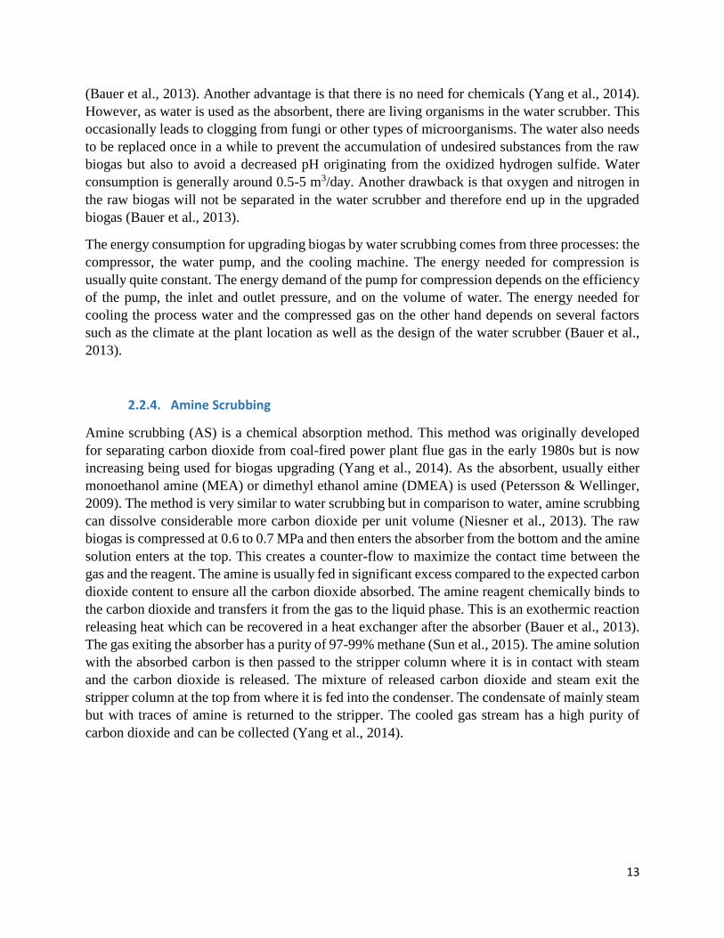
2.2.4. Amine Scrubbing

Amine scrubbing (AS) is a chemical absorption method. This method was originally developed

for separating carbon dioxide from coal-fired power plant flue gas in the early 1980s but is now

increasing being used for biogas upgrading (Yang et al., 2014). As the absorbent, usually either

monoethanol amine (MEA) or dimethyl ethanol amine (DMEA) is used (Petersson & Wellinger,

2009). The method is very similar to water scrubbing but in comparison to water, amine scrubbing

can dissolve considerable more carbon dioxide per unit volume (Niesner et al., 2013). The raw

biogas is compressed at 0.6 to 0.7 MPa and then enters the absorber from the bottom and the amine

solution enters at the top. This creates a counter-flow to maximize the contact time between the

gas and the reagent. The amine is usually fed in significant excess compared to the expected carbon

dioxide content to ensure all the carbon dioxide absorbed. The amine reagent chemically binds to

the carbon dioxide and transfers it from the gas to the liquid phase. This is an exothermic reaction

releasing heat which can be recovered in a heat exchanger after the absorber (Bauer et al., 2013).

The gas exiting the absorber has a purity of 97-99% methane (Sun et al., 2015). The amine solution

with the absorbed carbon is then passed to the stripper column where it is in contact with steam

and the carbon dioxide is released. The mixture of released carbon dioxide and steam exit the

stripper column at the top from where it is fed into the condenser. The condensate of mainly steam

but with traces of amine is returned to the stripper. The cooled gas stream has a high purity of

carbon dioxide and can be collected (Yang et al., 2014).

14

Figure 6: Process Flow Diagram of an Amine Scrubber (Bauer et al., 2013)

A major advantage of amine scrubbing is the high absorption capacity and rate (Xu et al., 2015).

Besides, there are almost no losses of methane in the process as the amine reacts selectively with

the carbon dioxide. The losses account for less than 1% (Sun et al., 2015). Amine scrubbing is

therefore preferred where strict environmental regulations on methane emissions are in place

(Yang et al., 2014). As the pH of the solution is quite high, there is little to no risk of bacterial

growth inside the system (Sun et al., 2015). However, hydrogen sulfide needs to be removed in

advance due to poisoning of the chemical and corrosion to the equipment (Ryckebosch et al., 2011;

Xu et al., 2015). Generally, systems are designed to handle a maximum of only 300 ppm hydrogen

sulfide in the incoming raw gas (Bauer et al., 2013). The upgraded gas leaving the absorber usually

has to be dried using temperature swing adsorption, pressure swing adsorption or freeze drying

(Bauer et al., 2013). Another drawback is that during the process significant solvent degradation

and losses due to evaporation occur which requires replacement (Petersson & Wellinger, 2009; Xu

et al., 2015).

Due to the large amount of high temperature heat needed to regenerate the chemical solvents, the

process has high energy consumption (Sun et al., 2015). The lowest energy consumption per

normal cubic meter of raw biogas can be achieved at the lowest load and the highest energy

consumption is required for the lowest loads (Bauer et al., 2013).

2.2.5. Membrane Separation

Membranes have been used for landfill gas upgrading already since the beginning of the 1990s in

the USA, but much less selective membranes were used then which yielded lower methane

recovery (Bauer et al., 2013). The method is based on the selective permeability property of

membranes (Ryckebosch et al., 2011). High permeable impurities such as carbon dioxide,

hydrogen, ammonia, water and parts of the oxygen pass through the membrane as permeate while

the low permeable methane, is retained and can be collected at the end of the hollow column (Yang

15

et al., 2014). The permeation rate of molecules is mainly dependent on their size but also their

hydrophilicity (Bauer et al., 2013). The membranes are usually made of polymers like silicone

rubber or cellulose acetate (Niesner et al., 2013). Membranes have an estimated lifetime of around

5-10 years (Bauer et al., 2013).

Before the raw biogas enters the hollow fibers, it is passed through a filter that retains water, oil

droplets and aerosols which would otherwise negatively affect the performance of the membrane

(Petersson & Wellinger, 2009). The water needs to be removed to prevent condensation during

compression of the biogas. Hydrogen sulfide is usually also removed with activated carbon before

since it will not be sufficiently separated by the membrane (Bauer et al., 2013). If ammonia,

siloxanes and volatile organic carbons are expected in significant amounts, these components are

also commonly removed before the biogas upgrading process. Then the biogas is pressurized and

fed through the membrane column (Bauer et al., 2013).

Figure 7: Process Flow Diagram of Membrane Separation (Bauer et al., 2013)

Membrane separation is well known for its safety, scale up flexibility, simplicity of operation and

maintenance, low cost, and the fact that no hazardous chemicals are required (Sun et al., 2015;

Yang et al., 2014). However, in order to achieve a high purity of the methane, large losses of

methane are involved (Sun et al., 2015). This means that there is likely some methane in the off-

gas which needs to be removed. This is often done by oxidizing the methane to carbon dioxide in

a regenerative thermal oxidizer or the off-gas stream is used in a combined heat and power plant

(CHP) together with raw biogas (Bauer et al., 2013).

The energy consumption for a membrane upgrading plant is mainly determined by the energy

consumption of the compressor. The energy consumption of the compressor on the other hand

depends very little on the methane concentration in the raw biogas. Therefore, the energy

consumption is independent of the raw gas consumption if expressed as kWh/Nm3 of raw biogas.

To increase the methane concentration in the upgraded biogas, a larger membrane area and/or a

higher pressure is needed. This both increases the energy required. Thus, higher methane

concentrations are associated with increased energy consumption (Bauer et al., 2013).

16

2.2.6. Cryogenic Separation

The method of cryogenic separation is still under development but it has the potential to be very

promising in the future (Sun et al., 2015). A pilot plant has been in operation in the Netherlands

since the beginning of 2009 (Petersson & Wellinger, 2009). Cryogenic separation uses the fact that

different components of the biogas condensate at different temperatures. The temperature is

stepwise decreased in order to remove the different gases individually and to optimize the energy

recovery (Petersson & Wellinger, 2009). In the first step, the raw biogas is cooled to 6°C which

causes water vapor to partially condense. Also, most heavy organic components which are water

solvable leave the gas stream in this step. Then the gas is compressed to 2.5 to 3.5 MP. In step 2,

siloxane and the remaining water vapor are condensed at -25°C. A hydrogen sulfide filter is used

to oxidize hydrogen sulfide to elemental sulfur and then filter both sulfur and siloxanes out of the

gas stream. In a third step, the carbon dioxide is frozen and separated from the gas stream at a

temperature of -78.5°C. The liquid carbon dioxide leaving this step has a high purity and can thus

be used as a refrigerant or other valuable byproduct. Lastly, the remaining biogas is liquefied at

around -190°C so that methane is condensed into liquefied biogas. The remaining gas stream is

mainly nitrogen (Yang et al., 2014).

Figure 8: Process Flow Diagram of Cryogenic Separation (Yang et al., 2014)

The biggest advantage of this upgrading process is that it separates the raw biogas into several

final products of high purity. Cryogenic Separation is particularly of interest if the final product

should be LBG which can be used to LNG in vehicle fuels (Ryckebosch et al., 2011). This method

also does not need any addition of chemicals and therefore produces no waste water stream or

hazardous chemicals to be disposed of (Yang et al., 2014). However, large amounts of energy are

needed for cryogenic separation mostly related to compressing and cooling of the gas. This is a

major drawback of the system. But as the technology is still quite new, it is likely that methods for

reducing the energy requirements can be developed in the future (Sun et al., 2015).

17

3. Methods 3.1. Case Study Description

In the first part, this case study evaluates the environmental impact of an anaerobic digester

including pre-treatment, and the following biogas upgrade to remove the carbon dioxide and

increase the methane density. The second part of this case study is focused on the costs and

revenues associated in building and maintaining an aerobic digester and the biogas upgrading unit.

For both parts, the environmental and the economic analysis, the system was divided into two

different subsystems: Subsystem 1 is the anaerobic digestion of waste feedstock which produces

the raw biogas and digestate as the end products, and Subsystem 2 which is the upgrade of this

raw biogas into upgraded biogas. The possible Subsystem 3, the treatment of the digestate, is not

considered in this study. Therefore, the product from Subsystem 1 is the feedstock for Subsystem

2. The Subsystem 1 is a generic anaerobic digester and is the same for all the different upgrading

technologies. Subsystem 2 is different for each upgrading technology. The different upgrading

technologies investigated in this case study are water scrubbing, pressure swing adsorption, amine

scrubbing, membrane separation, and cryogenic separation.

Figure 9: The Subsystems evaluated in this Case Study

This case study is only concerned with the anaerobic digestion and the biogas upgrade. The

emissions and costs occurring upstream of the anaerobic digestion such as collection of the

feedstock are not considered. The upgraded biogas is then assumed to be sold and used to substitute

natural gas in the national gas grid. The further use of the digestate from the anaerobic digestion

is also not considered.

3.2. Life Cycle Assessment

3.2.1. Methodology

A Life Cycle Assessment (LCA) is an assessment of environmental and resource impacts caused

by the activities needed to fulfill a certain function, considering the entire life cycle from cradle to

the grave. Starting in the 1980s, LCA has been widely used in industry trying to reduce the

Subsystem 1:

Anaerobic Digestion

Subsystem 3:

Digestate Treatment

(not considered)

Subsystem 2:

Biogas Upgrading

18

environmental burden from production, use, and disposal of many products. In the past decade,

LCA has also been increasingly applied in waste management providing insights into the

environmental aspect of waste management. Life cycle assessment analyzing products, so called

product LCAs, typically focus on the production and the use stage. An LCA of waste management

on the other hand focuses particularly on the end-of-life of products (M. Z. Hauschild & Barlaz,

2011). Often, all emissions occurring in the life cycle of the product before the product becomes

waste are omitted and the “cradle” is regarded as the point of waste generation where the product

becomes waste. This practice is often called the “zero burden approach” (Nakatani, 2014). Figure

10 illustrates the differences in the system boundaries for a product LCA and a waste LCA.

Figure 10: Boundaries of LCI of Products vs LCI of Solid Waste (M. Z. Hauschild & Barlaz, 2011)

In the 1980s when LCA was still in its infancy, a number of studies were performed in several

European countries comparing different packaging systems for milk. Although they all tried to

answer the same question and compared more or less the same packaging technologies, they came

up with different conclusions as to which packaging system had the lowest environmental impact.

The need for a harmonization of the life cycle assessment was realized. The International Standards

Organization (ISO) developed standards for LCAs and its main elements (ISO 14040 to ISO 1443).

These standards were then superseded by the ISO 14040 and ISO 14044 in 2006. According to the

LCA standard ISO 14040, the framework of a life cycle assessment consists of four phases: goal

and scope definition, inventory analysis, impact assessment, and interpretation (M. Z. Hauschild

& Barlaz, 2011). The figure below shows the different phases and how they are connected to each

other. Each phase is described in more detail below.

19

Figure 11: Framework for Life Cycle Assessment (JRC European Commission, 2010)

Goal and Scope Definition

The goal definition explains the purpose of the study, the decision process to which it provides

environmental decision support and the different financing parties. It is important to define

precisely the types of questions that can be addressed by the life cycle assessment but also the

types of questions which the LCA cannot answer (M. Z. Hauschild & Barlaz, 2011).

The scope definition is based on the goal definition. In the first step, the object of the study is

defined by the function or service it provides. This is called the functional unit. The functional unit

is of importance as to compare different systems, they need to provide the same function to the

user. In a waste LCA, the functional unit should include the quantity of waste to be managed, the

composition of the waste, the duration of the waste management service, and the quality of the

waste management. In the next step of the scope definition, the system boundaries are defined.

This includes a detailed description of the life cycle of the waste entering the system and drawing

of boundaries between the waste management system and the environment, and a specification of

the individual waste management processes. Next, the assessment criteria applied in the impact

assessment phase of the LCA must be specified. Then, the time scale of the study should be

addressed, particularly the requirements on the future validity of the results. This may have

profound significance for the choice of technology for the processes in the system and for the data

collected during the inventory analysis. Lastly, the perspective of the LCA needs to be decided. In

an attributional approach aims at giving a picture of the impacts from the system as it is, whereas

a consequential approach aims at supporting a decision on whether to change the system or not

(M. Z. Hauschild & Barlaz, 2011).

20

Inventory Analysis

The inventory analysis collects information about the physical flows in terms of input of resources

and products and output of emissions and waste from the system. The analysis studies all the

processes that were identified as belonging to the product system (M. Hauschild, 2015a). In

general, data collection is based on mass balances for the processes over a long period of time to

ensure that the data are representative of the average functioning of the process. The flows then

are scaled in accordance with the functional unit, for example kg CO2-fossil/1000 kg of waste. The

quality of the data collected in the inventory is crucial to the outcome of the life cycle assessment.

Generally, the best data is that calculated by mass balances or obtained through measurements.

The collection of this kind of data is very time consuming and sometimes not even possible.

Therefore, it is necessary to use data that has been extrapolated from similar technologies

elsewhere or from other types of technologies. Also, sometimes the inventory analysis needs to

rely on generic data from databases for many processes such as the production of materials or

components, or the generation of electricity. The outcome of the inventory analysis is the life cycle

inventory (LCI) which is a list of quantified physical elementary flows for the product system

associated with the provision of the functional unit (M. Z. Hauschild & Barlaz, 2011).

Impact Assessment

The LCI will contain a large number of inputs and emissions. Only some of these exchanges are

environmentally significant and even small amounts can be of importance. The purpose of the

impact assessment is to interpret the inventory results into their potential impacts and effects by

applying the best available knowledge about relations between emissions and their effect on the

environment. Taking the life cycle inventory as the starting point, the life cycle impact assessment

(LCIA) translates the physical flows and interactions of the product system into the impacts on the

environment that can be associated with the functional unit of the study. This translation is done

in four steps. First, the impact categories are defined and the exchanges from the inventory are

assigned to impact categories according to their ability to contribute to different problem areas.

Some substances may contribute to more than one impact category. This step is called

classification. Then, in the characterization step, the contributions of the emissions to the different

impact categories are quantified. The resulting characterized impact scores are expressed in a

common metric for the impact category. This allows for aggregations of all contributions into one

score which represents the overall impact for that category. Then, the impact categories are put on

a common scale by relating them to a common set of references in a step called normalization.

This shows the relative magnitudes of the characterized scores and allows for determining which

impacts are large and which are small relative to the reference impact. The result of this step is the

normalized impact profile in which all category indicator scores are expressed in the same metric.

Lastly, valuation allows for ranking, grouping, or assignment of weights to the different impact

potentials. According to ISO 14040, the first wto steps of the impact assessment are mandatory

while the last two are optional (M. Z. Hauschild & Barlaz, 2011).

21

LCIA methods exist for midpoint and for endpoint level. In midpoint modelling the impacts are

modelled until some midpoint in the environmental mechanism (M. Z. Hauschild & Barlaz, 2011).

There are also a higher number of impact categories differentiated (typically around 10 to 15) and

the results are more accurate and precise compared to the endpoint level. Typical midpoint impact

categories include climate change, stratospheric ozone depletion, human toxicity, ionizing

radiation, photochemical ozone formation, acidification, eutrophication, ecotoxicity, land use, and

resource depletion (JRC European Commission, 2010). In endpoint modelling, the impacts are

modelled all the way to effects on the so-called areas of protection using the best available

environmental models. Some believe that the increased uncertainty is warranted by the improved

interpretation of the results. The three areas of protection are human health, natural environment,

and natural resources (M. Z. Hauschild & Barlaz, 2011). The figure below shows different

midpoints and the endpoints and how the midpoints contribute to the three areas of protection.

Figure 12: Midpoints and Endpoints and their Connections (M. Hauschild, 2015b)

Interpretation

The results of the study are interpreted while considering the questions posed in the goal definition

and the limitations defined in the scope definition (M. Hauschild, 2015a). The outcome of the

interpretation may be a recommendation to decision makers, who will normally weight it against

other decision criteria such as economic or social aspects (M. Z. Hauschild & Barlaz, 2011).

Sensitivity analysis and uncertainty analysis are also applied as part of the interpretation to qualify

the conclusions that are drawn from the results, to appraise the strength of the conclusions, and to

identify the focus points for further work in order to increase the strength of the conclusion. The

sensitivity analysis identifies the key figures of the LCA, meaning those model assumptions,

processes and environmental exchanges that have the greatest bearing on the study results. The

significance of uncertainty in key data can be determined by letting them vary within their

estimated range and examining the effect of these variations on the results (M. Z. Hauschild &

Barlaz, 2011).

22

Even though it was mentioned that a life cycle assessment consists of four consecutive phases, an

LCA is an iterative process where experience gathered in a later phase may serve as feedback

leading to modifications of one or more of the earlier phases. In Figure 11, the arrows indicate the

interaction between the different phases. Insights from the impact assessment are used in refining

the inventory analysis and knowledge from both of these phases may feed back to the scope

definition. Therefore, each phase provides feedback to the previous phases and helps target the

next iteration of the LCA. The first iteration is often an initial screening, covering the full life

cycle, but the inventory data is mostly based on easily accessible data from databases. Then

following the impact assessment, the parts of the product system that contribute most strongly to

the total result are identified. These are key figures and their data should be the target of the next

iteration, where the main focus lies on finding more representative or recent inventory data. Based

on the revised inventory, a new impact assessment is performed, and the sensitivity analysis

performed once more to see which are now the key figures and main assumptions. The uncertainty

of the results is reduced with each iteration, until the remaining uncertainty of the results is

sufficiently small to meet the goal of the study (M. Hauschild, 2015a). The figure below shows

the iterative approach in performing an LCA.

Figure 13: Iterative Approach of a Life Cycle Analysis (M. Hauschild, 2015a)

3.2.2. The Model

For this study, an LCA was conducted following the ISO 14040 standard. The life cycle assessment

was done using the program EASETECH developed at the Danish Technical University (DTU) in

Copenhagen. EASETECH is specifically designed to perform life cycle assessments of complex

systems handling heterogeneous material flows (DTU, 2017).

The objective of this study is to determine the environmental impact of different biogas upgrading

technologies. The biogas is assumed to be produced by a wet thermophilic anaerobic digester for

all scenarios. The different upgrading technologies which were examined are PSA, water

scrubbing, amine scrubbing, membrane separation, and cryogenic separation.

23

The input into the subsystem 1, is organic household waste. The waste then undergoes a pre-

treatment to sort out unwanted impurities. What happens to these impurities is outside the scope

of this study and not further investigated. The rest of the organic waste is used as the feedstock for

the anaerobic digester. The anaerobic digestion produces raw biogas and a solid product called

digestate. The digestate can be used as a fertilizer on agricultural field. However, this is not further

evaluated in this study. The biogas is assumed to consist only of 65% methane and 35% carbon

dioxide. Other impurities such as hydrogen sulfide, nitrogen or hydrogen are neglected as there

was not enough data available. Up to here, it is the first subsystem and is the same for all different

scenarios. Even though the anaerobic digestion process is the same for all the different upgrading

technologies, it was chosen to include it anyway to give a perspective of the environmental impact

of the anaerobic digestion compared to the upgrading technologies.

Subsystem 2 is different for each biogas upgrading technology evaluated. The five technologies

which are analyzed are pressure swing adsorption, water scrubbing, amine scrubbing, membrane

separation, and cryogenic separation. Each technology uses a different technique to separate the

methane from the carbon dioxide of the raw biogas. The desired product of this process is the

upgraded biogas containing mainly methane. The process also produces stream of mainly carbon

dioxide which is either vented off or used depending on the purity. The upgraded biogas is then

compressed to the same pressure as the natural gas in the national gas grid. The compressed biogas

can then be injected into the gas grid where it substitutes natural gas.

The infrastructure for the different technologies are not considered in this analysis as it is assumed

to be the same for the different upgrading technologies. The figure below shows the model used

for the life cycle assessment including the system boundaries.

Figure 14: Model for Life Cycle Assessment

The functional unit (FU) is the treatment of 1 ton (1000 kg) of municipal organic waste. The biogas

produced by anaerobic digestion is upgraded to natural gas quality so it can be injected into the

national gas grid.

24

3.2.3. Data Collection

As no data from a specific plant was available the values used in the life cycle assessment were

collected through a literature study and adjusted as much as possible to the geographical scope of

the United States. The upgrading technologies were selected based on the data available, especially

for electricity used, quality of the upgraded biogas, and the methane slip.

3.2.3.1. Anaerobic Digestion

The modelling of the waste generation and the anaerobic digestion is the same for all the different

upgrading technologies. These include the waste generation (“Disposed Household Organic

Waste”), the removal of impurities (“Pre-Treatment”), the anaerobic digestion process (“biogas

production, thermophilic”), the leaking of methane (“Leaking CH4”), and fugitive emissions of

methane (“Fugitive emissions CH4”).

Disposed Household Organic Waste

The composition of the municipal solid waste used for the life cycle assessment is based on data

from California of multi-family and single-family residential disposed waste. In 2011 California

set the goal of recycling 75 percent of its waste by 2020 to statewide decrease the reliance on

landfills. An important part of this mission is to increase the diversion of organic materials away

from landfills and toward the production of value-added products (CalRecycle, 2017). In order to

measure the progress of this goal, California periodically conducts statewide waste

characterization studies based on types and amounts of materials in the waste stream. Studies were

conducted in 1999, 2004, 2006, 2008, and 2014 (CalRecycle, 2016). As there is detailed data

available for California, this data was taken for the life cycle analysis and it was assumed that the

data is representative for the whole United States. The most recent data from 2014 was taken which

provides data for the quantity and composition of the residential waste streams.

Data was taken from multi-family residential disposed waste and single-family disposed waste to

create a single stream of household organic waste. Organic waste makes up 43.8% of the waste

from multi-family residential disposed waste, and 45.7% of single-family residential disposed

waste. By adding up the estimates of each waste fraction, the relative percentage of each fraction

to the total organic waste was calculated. The data from CalRecycle provides data for eight

different waste fractions. For each of these fraction, a corresponding material fraction was

chosen in EASETECH.

Table 2 shows each waste fraction from CalRecycle and the corresponding material fraction which

was used in EASETECH as well as the calculated percentage of each fraction to the total organic

waste.

25

Table 2: Material Fractions used for “Disposed Household Organic Waste” in EASETECH

Waste Fraction from CalRecycle Material Fraction used in EASETECH Percentage

Food Vegetable Food Waste 49.89%

Leaves and Grass Garden Waste, Grass and Leaves 10.40%

Prunings and Trimmings Garden Waste, Plants 8.67%

Branches and Stumps Garden Waste, Branches 0.34%

Manures Slurry Cow Manure 0.05%

Textiles Textiles 12.48%

Carpet Other non-combustibles 3.43%

Remainder/Composite Organic Other combustibles 14.74%

Pre-Treatment

For the pre-treatment, values from Naroznova, Møller, Larsen, & Scheutz (2016) were taken. In

the article, a new technology for pre-treating source-separated organic household waste prior to

anaerobic digestion is assessed. A table lists the transfer of different material fractions from the

initial source separated organic household waste to the feedstock for the anaerobic digester based

on percent total on a dry weight basis (Naroznova, Møller, Larsen, & Scheutz, 2016). The same

values were assumed to be true for a generic pre-treatment.

The table below lists the waste fractions and the corresponding amount of each fraction going to

the feedstock which is then sent to the anaerobic digester. The table only lists the material fractions

which were mentioned in “Disposed Household Organic Waste” above and used in for the waste

generation. The article lists other material fractions as well, but as these were not used in this study,

they are therefore omitted here.

For “vegetable food waste”, “manure”, “textiles”, and “other combustibles” values were available

directly for this material fraction. For “grass and leaves”, “plants”, and “branches” no exact values

for this material fraction, so the value for “yard waste, flower” was taken for all of them. For “other

non-combustibles” the same value as for “other combustibles” was taken.

Table 3: Transfer of material fractions from organic waste to feedstock (Naroznova et al., 2016)

Material Fraction % total (dry weight basis)

Vegetable Food Waste 95

Garden Waste, Grass and Leaves 84

Garden Waste, Plants 84

Garden Waste, Branches 84

Slurry Cow Manure 98

Textiles 3

Other non-combustibles 11

Other combustibles 11

26

Biogas Production, thermophilic

The anaerobic digester was assumed to be a wet, one stage, thermophilic process. Wet means that

the process has a moisture of content above 90%. One stage means that the initial hydrolysis and

acidification take place in the same reactor as the methane production. And a thermophilic process

has a temperature of around 53-55°C (Angelidaki, 2004). The process “Biogas production,

Thermophilic, Generic, 2007” from the EASETECH database was used and adjusted as described

below.

The gas yield as a proportion of degradable carbon and the loss of VS related to the loss of biogenic

carbon were left at the default values of 70 and 1.89 respectively. The measured methane

percentage in the biogas was assumed to be 65% which is consistent with the general composition

of biogas from anaerobic digestion (Sun et al., 2015). For simplicity, it is assumed that the biogas

only consists of methane and carbon dioxide. Therefore, no removal of impurities is necessary

before applying the upgrading technology.

For the external processes, the default amounts of electricity and heat were not changed, but

adjusted to the geographical area of the United States. The process used for the electricity was

“market group for electricity, medium voltage; US”. 18.3 kWh/ton total wet weight (WW) is used

for pumps, ventilator, etc. and 30.6 kWh/ton total wet weight is used for heating of the reactor

(Damgaard, Baumeister, Astrup, & Christensen, 2016). The external process used for the heat

requirements was “heat and power co-generation, natural gas, conventional power plant, 100MW

electrical; WECC, US only”. 90% of the wet weight was assumed to consist of water and the

energy used to heat the water to 55°C is (55-11.5)*4.2*0.9/1000 MJ/kg total wet weight or 0.164

MJ/kg total wet weight (Damgaard et al., 2016), where 11.5 is the average annual temperature in

the United States (Weatherbase, 2017) and 4.2 is the specific heat of water. The other 10% are

assumed to be solids and the energy used to heat up the solids is (55-11.5)*3*0.1/1000 MJ/kg total

wet weight or 0.013 MJ/kg total wet weight, where 3 is the specific heat of the solids (Damgaard

et al., 2016).

The two processes “market group for electricity, medium voltage; US” and “heat and power co-

generation, natural gas, conventional power plant, 100MW electrical; WECC, US only” were

imported from the ecoinvent database to represent the geographical scope of the United States.

The diesel used for the machinery at the plant was left at the default process “Wheel loader,

combustion 1L of diesel, 2008/2011” at the default amount of 0.0009 L/kg total wet weight

(Damgaard et al., 2016).

27

Table 4: External Processes used for “Biogas Production, Thermophilic”

Category Process Amount Unit

Electricity market group for electricity, medium voltage;

US

0.049 kWh/kg total ww

Heat for Water heat and power co-generation, natural gas,

conventional power plant, 100MW electrical;

WECC, US only

0.164 MJ/kg total ww

Heat for Solids heat and power co-generation, natural gas,

conventional power plant, 100MW electrical;

WECC, US only

0.013 MJ/kg total ww

Diesel Wheel loader, combustion 1L of diesel,

2008/2011

0.0009 L/kg total ww

Leaking CH4

Some methane is lost due to leaking of the digester. These losses are difficult to measure. IPCC

gives a range of 0-10% of produced methane (Møller, Boldrin, & Christensen, 2009), whereas the

losses are around 2% according to Swedish experiences (Börjsson, 2008). The leaking of methane

from the anaerobic digester was therefore set to 2%.

Fugitive Emissions CH4

The 2% of methane described in the “Leaking CH4” before is emitted into the atmosphere. These

emissions are defined with the transformation “Methane, non-fossil” as the methane is produced

from food waste, wood and yard trimmings which are renewable resources.

3.2.3.2. Pressure Swing Adsorption

The raw biogas is upgraded using PSA. The model includes the biogas upgrading (“PSA”), the

release of the waste stream containing mainly carbon dioxide (“venting off-gases”), the

compression of the gas to the pressure of the national gas grid (“Gas Compression”), losses that

occur during the distribution of the biogas (“Gas Distribution Losses”), and the substitution of

natural gas with biogas (“Substitution of Natural Gas”).

PSA

Pressure Swing Adsorption only requires electricity but does not require any heat. The electricity

is composed of electricity for upgrading which is 0.2 kWh per Nm3 of raw biogas, and the

electricity for drying and compression which is 0.17 kWh per Nm3 upgraded biogas or 0.11 kWh

per Nm3 raw biogas (Bauer et al., 2013). Therefore, the total electricity required for PSA is 0.31

28

kWh/Nm3 raw biogas. The process “market group for electricity, medium voltage; US” was chosen

as the external process for electricity consumption.

Table 5: External Processes used for “PSA”

Category Process Amount Unit

Electricity for

upgrading

market group for electricity, medium

voltage; US

0.2 kWh/m3 volume

Electricity for

drying and

compression

market group for electricity, medium

voltage; US

0.11 kWh/m3 volume

Bauer et al. (2013) report a methane slip of 1.6%, meaning that 1.6% of the methane in the raw

biogas is assumed to end up in the carbon dioxide stream and 98.4% of the methane ends up in the

upgraded biogas. For the methane purity of the upgraded biogas Sun et al. (2015) reports values

ranging from 95-99% and Niesner et al. (2013) reports a methane purity of 98%. The value of 98%

for the methane purity was chosen as this also lies within the values reported by Sun et al. (2015).

The carbon dioxide slip can be calculated with the following formula derived in Appendix II:

z = (0.65

0.35∗ (100 − 𝑚)) ∗ (

100

𝑝 − 1)

where:

z: carbon dioxide slip

m: methane slip

p: methane purity of upgraded biogas

Inserting the values for methane slip (m=1.6) and methane purity of the upgraded biogas (p=98)

into the equation gives the following:

z = (0.65

0.35∗ (100 − 1.6)) ∗ (

100

98 − 1) = 3.7

Therefore, the carbon dioxide slip is 3.7%.

Venting off-gases

The off-gases from the biogas upgrading, meaning most of the carbon dioxide as well as the

methane that slips into the carbon dioxide stream, are assumed to be vented into the atmosphere.

The emissions of methane and carbon dioxide are exchanged at 100% as “Methane, non-fossil”

and “Carbon dioxide, non-fossil” respectively.

29

Gas Compression

As no data was found regarding gas compression, the default value of 0.065 kWh/m3 CH4 and

0.065 kWh/m3 CO2 from the EASETECH software was taken. The process was also adjusted to

the geographical scope of the United States by using the external process “market group for

electricity, medium voltage; US”.

During the distribution of the biogas, it is assumed that losses of 2% occur (Damgaard et al., 2016).

Gas Distribution Losses

Like for the fugitive emissions from the leaked biogas during the anaerobic digestion and for the

venting of the off-gases from the upgrading process, it is again assumed that the methane in the

biogas is to 100% transformed into “methane, non-fossil” and the carbon dioxide is transformed

into “carbon dioxide, non-fossil”.

Substitution of Natural Gas

The upgraded biogas can be used to substitute natural gas in the national natural gas grid. The

process “market for natural gas, high pressure; US” was used as the substituted external process.

The substitution was assumed to be based on the volume of the biogas.

3.2.3.3. Water Scrubbing

The raw biogas is upgraded using the water scrubbing technology. The model includes two

processes needed to create the water in EASETECH (“create m3 Volume” and “adding water”), as

well as the biogas upgrading (“Water Scrubbing”), the treatment of the waste water (“Waste Water

Treatment”), the release of the waste stream containing mainly carbon dioxide (“venting off-

gases”), the compression of the gas to the pressure of the national gas grid (“Gas Compression”),

losses that occur during the distribution of the biogas (“Gas Distribution Losses”), and the

substitution of natural gas with biogas (“Substitution of Natural Gas”).

Create “m3 Volume”

This process and the following are only to trick the EASETECH software. The first one creates

the “m3 Volume” from the sum of the volume of methane and the volume of carbon dioxide.

30

Adding Water

This process adds water as the EASETECH software does not automatically create water when an

external process water is added. Water usage is between 0.5-5 m3 per day (Bauer et al., 2013).

Generally, water scrubbing is applied for a biogas flow of 100-2000 Nm3/h (Niesner et al., 2013).

Assuming a 24h operation per day, this would result in a water consumption of 0.0002 m3/Nm3

raw biogas ((0.5 m3/day) / (24 h/day) / (100 Nm3 biogas/h)) for the lower end of the biogas flow

and water consumption, and 0.0001 m3/Nm3 raw biogas ((5 m3/day) / (24 h/day) / (2000 Nm3

biogas/h)) for the higher end. The medium value of 0.00015 m3/Nm3 was used.

Water Scrubbing

The water scrubbing biogas upgrading technology requires only electricity but no heat. The

electricity consumption for water scrubbing comes from three activities: compression, water pump

and cooling system. Compression requires between 0.1-0.15 kWh/Nm3 raw biogas, the water

pump requires between 0.05-0.1 kWh/Nm3 raw biogas, and the cooling system requires between

0.01-0.05 kWh/Nm3 raw biogas (Bauer et al., 2013). A value in the middle of the interval was

chosen for each source which means 0.12 kWh/Nm3 raw biogas for compression, 0.07 kWh/Nm3

raw biogas for water pumping, and 0.03 kWh/Nm3 raw biogas for the cooling system. Adding the

three energy requirements up gives a total required electricity per Nm3 raw biogas of 0.22 kWh.

The external process “market group for electricity, medium voltage; US” was again used to

represent the electricity consumption.

Electricity and water is used for water scrubbing. Unfortunately, there is no process available in

ecoinvent for water consumption in the United States. So the process for water in the Canadian

province of Quebec “market for tap water; CA-QC” was used, as this was assumed to be very

similar to the United States.

Table 6: External Processes used for “Water Scrubbing”

Category Process Amount Unit

Electricity for

compression

market group for electricity, medium

voltage; US

0.12 kWh/m3 volume

Electricity for

water pump

market group for electricity, medium

voltage; US

0.07 kWh/m3 volume

Electricity for

cooling system

market group for electricity, medium

voltage; US

0.03 kWh/m3 volume

Water

Consumption

market for tap water; CA-QC 0.001 m3 Water/kg

Water

Methane losses for Water Scrubbing of between 1-2% are reported by Sun et al. (2015). A value

of 1.5% for the methane slip was therefore chosen as it lies in the middle of this range. Niesner et

al. (2013) reports a methane purity of around 98% and Sun et al. (2015) reports values of between

31

95 and 99%. The value of 98% was chosen. Using these values, the carbon dioxide slip is 3.7%

based on calculations derived in Appendix II

Waste Water Treatment

The waste water from the water scrubbing needs to be treated. As only a waste water treatment

plant for landfill leachate was available in EASETECH, this process has been taken (Leachate –

Treatment – Avedøre WWTP (3a) emission to surface water). The values were left the same only

the electricity was changed to the geographical scope of the United States. The default values

assume that 5.5% of the COD is in the effluent and 90% of the biogas is used for electricity with

3.48 kWh/kg COD. These values were not changed. The process nor the values were changed for

the process water

Table 7: External Processes used for "Waste Water Treatment"

Category Process Amount Unit

Electricity for

biological and

mechanical

treatment

market group for electricity, medium

voltage; US

0.000443 kWh/kg Total

Wet Weight

biogas used for

electricity

market group for electricity, medium

voltage; US

-0.945*0.9*3.48 kWh/kg COD

Process Water Process water from surface water,

RER, 2005, ELCD

3.19E-08 kg/kg Total

Wet Weight

Gas Compression, Venting off-gases, Gas Distribution Losses & Substitution of Natural Gas

The processes “Gas Compression”, “Venting off-gases”, “Gas Distribution Losses” and

“Substitution of Natural Gas” are the same as for the Pressure Swing Adsorption scenario.

3.2.3.4. Amine Scrubbing

In this scenario, the raw biogas is upgraded using the amine scrubbing technology. In addition to

the anaerobic digestion, the model includes the processes needed to create the water in

EASETECH (“create m3 Volume” and “adding water”), as well as the biogas upgrading (“Amine

Scrubbing”), the treatment of the waste water (“Waste Water Treatment”), the release of the waste

stream containing mainly carbon dioxide (“venting off-gases”), the compression of the gas to the

pressure of the national gas grid (“Gas Compression”), losses that occur during the distribution of

the biogas (“Gas Distribution Losses”), and the substitution of natural gas with biogas

(“Substitution of Natural Gas”).

32

Create m3 Volume, adding water & Waste Water Treatment

The processes “create m3 Volume”, “adding water”, and “Waste Water Treatment” are the same

as described in 3.2.3.3 Water Scrubbing, except that 0.0003 kg Water is used per m3 Volume.

Amine Scrubbing

The Water Scrubbing upgrading technology requires electricity, heat, water and chemicals. 0.55

kWh heat is required per Nm3 of raw biogas (Bauer et al., 2013). The process “market for heat,

district or industrial, natural gas; CA-QC”. The process for Canada – Quebec was chosen, as no

suitable process representing the United States was found. This process is in units of MJ, therefore

the required heat needs to be converted to MJ by multiplying it with 3.6 MJ/kWh (so 0.55

kWh/Nm3 * 3.6 MJ/kWh = 1.98 MJ/Nm3).

Bauer et al. (2013) also states that 0.14 kWh of electricity is required per Nm3 of raw biogas treated

at lowest load or 0.12 kWh/Nm3 raw biogas at highest load. A medium value of 0.13 kWh/Nm3

raw biogas was chosen. As before, the process “market group for electricity, medium voltage; US”

was used to represent the required electricity.

As mentioned before, Amine Scrubbing also requires water. Bauer et al. (2013) reports a water

consumption of 0.00003 m3/Nm3 of raw biogas. Again, no process for the United States was found,

therefore the process “market for tap water; CA-QC” for Quebec was used again as for water

scrubbing.

The chemical consumption is given in Bauer et al. (2013) as 0.00003 kg/Nm3 raw biogas and

includes anti foam agents and the amine make up. For simplicity, it was assumed that the chemical

consumption only consists of the amine make up used as the absorbent. Usually either mono

ethanol amine (MEA) or dimethyl ethanol amine (DMEA) is used (Petersson & Wellinger, 2009).

For DMEA, no process could be found in the ecoinvent database, therefore it was assumed that

MEA is used as the amine absorber. The process “market for monoethanolamine; GLO” was used.

GLO means the global dataset and represents what is considered to be the average production

(Ecoinvent, 2017).

Table 8: External Processes used for “Amine Scrubbing”

Category Process Amount Unit

Heat market for heat, district or industrial,

natural gas; CA-QC

0.55*3.6 MJ/m3 volume

Electricity market group for electricity, medium

voltage; US

0.13 kWh/m3 volume

Water

Consumption

market for tap water; CA-QC 0.001 m3 Water/kg

Water

Chemicals market for monethanolamine; GLO 0.00003 kg/m3 volume

33

The methane slip for amine scrubbing is very low (<0.1% (Petersson & Wellinger, 2009), 0.1-

0.2% (Sun et al., 2015), 0.06% (Bauer et al., 2013)) as suggested by several sources. To be

consistent with the sources, the value from Bauer et al. (2013) of 0.06% was used. Bauer et al.

(2013) do not mention any purity of the upgraded biomethane. However, Sun et al. (2015) report

purities of 97 to 99% of methane by volume. A purity of 98% was chosen for the upgraded biogas

as this lies in the middle of the range. This results in a carbon dioxide slip of 3.8%

Gas Compression, Venting off-gases, Gas Distribution Losses & Substitution of Natural Gas

The processes “Gas Compression”, “Venting off-gases”, “Gas Distribution Losses” and

“Substitution of Natural Gas” are the same as for the Pressure Swing Adsorption scenario.

3.2.3.5. Membrane Separation

Membrane Separation is used in this scenario to upgrade the raw biogas from the anaerobic

digester into upgraded biogas. Adding on to the anaerobic digestion described in section 3.2.3.1,

the scenario includes the biogas upgrading (“Membrane Separation”), the release of the waste

stream containing mainly carbon dioxide (“venting off-gases”), the compression of the gas to the

pressure of the national gas grid (“Gas Compression”), losses that occur during the distribution of

the biogas (“Gas Distribution Losses”), and the substitution of natural gas with biogas

(“Substitution of Natural Gas”).

Membrane Separation

Membrane Separation only requires electricity. The energy consumption is mainly due to the

compressor and depends very little on the methane concentration in the raw biogas (Bauer et al.,

2013). Bauer et al. (2013) report an electricity demand in the interval 0.2 to 0.3 kWh/Nm3 of raw

biogas, and Sun et al. (2015) notes an electrical energy consumption of 0.15 to 0.22 kWh/Nm3 raw

biogas. An electricity consumption of 0.2 kWh/Nm3 raw biogas was chosen for the calculation as

it is in the overlap of the two sources. Again, the external process “market group for electricity,

medium voltage; US” was chosen.

Table 9: External Processes used for “Membrane Separation”

Category Process Amount Unit

Electricity market group for electricity, medium

voltage; US

0.2 kWh/m3 volume

The methane losses during Membrane Separation are mentioned to be substantial (Bauer et al.,

2013; Petersson & Wellinger, 2009) but only Sun et al. (2015) quantifies the methane losses with

values of between 2 and 13.5%. A value of 8% for the methane slip was chosen but there is a

significant uncertainty associated with this. For the methane concentration of the upgraded biogas,

34

Bauer et al. (2013) report methane concentrations of above 98% whereas Sun et al. (2015) reports

values of 90-99%. Niesner et al. (2013) reports that methane purity of 90-97% in single stage

systems and purity of up to 99% for multistage systems. A methane purity of 96% for the upgraded

biogas was chosen. This is on the rather high end for a single stage system but achievable for

multistage systems. Again, there is a high uncertainty associated with this value. Based on these

values, the carbon dioxide slip is 7.1%

Gas Compression, Venting off-gases, Gas Distribution Losses & Substitution of Natural Gas

The processes “Gas Compression”, “Venting off-gases”, “Gas Distribution Losses” and

“Substitution of Natural Gas” are the same as for the Pressure Swing Adsorption scenario.

3.2.3.6. Cryogenic Separation

In this scenario, the raw biogas is upgraded using Cryogenic Separation. The model includes the

biogas upgrading (“Cryogenic Separation”), the release of the waste stream containing mainly

carbon dioxide (“venting off-gases”), the distribution of the gas to the national gas grid (“Gas

Distribution”), losses that occur during the distribution of the biogas (“Gas Distribution Losses”),

and the substitution of natural gas with biogas (“Substitution of Natural Gas”).

Cryogenic Separation

Cryogenic separation has a high energy consumption due to the high pressure and very low cooling

temperatures. The energy demand reported by Bauer et al. (2013) is 0.76 kWh/Nm3 of raw biogas.

Sun et al. (2015) reports values of between 0.2-1.05 kWh/Nm3 raw gas based on calculation. The

value from Bauer et al. (2013) was chosen here as it also lies within the value reported by Sun et

al. (2015). Again, the external process “market group for electricity, medium voltage; US” was

used. No heat, water or chemicals are used.

Table 10: External Processes used for “Cryogenic Separation”

Category Process Amount Unit

Electricity market group for electricity, medium

voltage; US

0.76 kWh/m3 volume

The methane slip is reported to be lower than 1% by Sun et al. (2015) and even between 0.037-

0.5% as reported by Bauer et al. (2013). The value of 0.5% was chosen. The methane purity is

very high and reported to be 99% by Yang et al. (2014). Therefore, the carbon dioxide slip is 1.9%.

35

Substitution of liquid Carbon Dioxide

The liquid and pressurized carbon dioxide leaving the Cryogenic Separation is very pure (>99%).

It can therefore be used as a refrigerant or other valuable byproduct (Yang et al., 2014). The process

“carbon dioxide production, liquid; RoW” was used as the substituted external process. As this

process is based on kg but the flow of biogas is in m3, the weight of the byproduct (the carbon

dioxide) needs to be calculated.

Carbon dioxide gas has a density of 1.977 kg/m3 at 1 atm and 0°C (Wikipedia, 2017). Therefore,

each m3 of carbon dioxide gas substitutes 1.977 kg of carbon dioxide. The substitution was

assumed to be based on the volume of the carbon dioxide.

Gas Distribution

The upgraded biogas does not need compression as it is already compressed during the upgrading.

However, it is again assumed that losses of 2% occur during the distribution.

Substitution of Natural Gas

The process “Substitution of Natural Gas” is the same as for the Pressure Swing Adsorption.

3.3. Cost Evaluation

3.3.1. Methodology

A new project involves spending an investment, I, and then earing a return, R, over time. For

example, the construction of an anaerobic digester or a biogas upgrading plant requires spending

of money now in the hopes of earning money subsequently. However, money earned in the future

has not the same value as money now. There are several reasons why a promise of future payments

is not worth the same value today. Some of it involves the risk that the money may not be paid.

But even with leaving risk aside, most people prefer $1 today to $1 payable in a year. One way of

expressing this is that the present value of a payment of a dollar in the future is less than a dollar.

So from a present value perspective, future payments are discounted (McAfee, Lewis, & Dale,

2006).

One way of analyzing and comparing different investment options is by calculating the net present

value for each project. The net present value (NPV) is the present value of a stream of net

payments. The NPV approach involves assigning a rate of return, r, that is reasonable for the

project and then computing the present value of the expected stream of payments. Since the

investment is initially expected, it is counted as a negative revenue. The formula for calculating

the net present value is given as following (McAfee et al., 2006):

36

𝑁𝑃𝑉 = −𝐼 + 𝑅1

1+𝑟+

𝑅2

(1+𝑟)2 + ⋯

where:

I: initial investment

r: rate of return

R1: first year revenues

R2: second year revenues, and so on…

The net present value is therefore used to analyze an investment decision and give the firm a clear

way to tell if the investment will add value to the company. If the NPV is positive, it adds to the

net value of the firm and therefore should be considered. If the value is negative, the project should

be dismissed (InvestingAnswers, 2017).

3.3.2. The Model

The cost evaluation for different upgrading technologies was done using the net present value as

described above. All the calculations were done using Microsoft Excel. The raw biogas is assumed

to consist of 65% methane and 35% carbon dioxide. The objective of this study was to determine

which upgrading technology is the most cost efficient over a certain time span. In order to do this,

the initial investment cost, the year costs for maintaining the plant, and the incomes from the sale

of products was considered. These costs and revenues were available for plants of different sizes

which allowed for extrapolation of the costs for plants of other flow ranges as well. Again, the

analysis was divided into a first subsystem which considers the anaerobic digestion and is the same

for all the scenarios. Then, in subsystem 2, three different biogas upgrading technologies are

studied. These technologies are PSA, water scrubbing and amine scrubbing.

For subsystem 1, an initial investment is required for building the anaerobic digester and all the

equipment associated with it. This is a one-time cost to be paid before construction of the digester.

The initial investment is spilt up into different categories which all contribute to the investment

cost. Additionally, there are also yearly costs in order to keep the digester running. Again, there

are different categories of costs which are added up to the total yearly costs. These costs occur

each year and are discounted accordingly. Besides the initial investment and the yearly costs, there

are also revenues. One kind of income comes from the tipping fees. This means that the city or

private parties pay the company running the digester to take their organic food waste. Also,

revenue can be achieved through the sale of the digestate which can be used as a fertilizer by

farmers or homeowners. Both of these revenues occur yearly and are therefore discounted

accordingly.

37

Figure 15: Anaerobic Digestion Model for Cost Evaluation

For the different biogas upgrading units in subsystem 2, there is also an initial investment required

for constructing the plant. Again, this is a one-time payment before the plant is built. The total

investment cost is divided up into different categories each contributing to the total. In order to

keep the plant running, there are also yearly costs which are made up of different categories. These

costs occur yearly and are therefore discounted to the present value. Revenue is generated through

the sale of upgraded biogas. The biogas is sold to the utility managing the gas grid where it is used

to substitute natural gas. Income from the biogas is a yearly revenue and is therefore also

discounted in order to calculate the net present value. The figure below shows the model used to

calculate the costs and revenues for the different biogas upgrading technologies.

Figure 16: Biogas Upgrading Model for Cost Evaluation

38

3.3.3. Data Collection

Detailed data was available for an anaerobic digester plant and three different biogas upgrading

plants. The three technologies for which data was available to conduct the cost evaluation are

pressure swing adsorption, amine scrubbing and water scrubbing. For membrane separation only

data for the investment cost was available and for cryogenic separation no data was available.

Therefore, it was not possible to conduct the cost evaluation on these two technologies.

The cost data was taken from Urban (2008). As the data is form 2008, inflation was accounted for

to accurately describe today’s situation. An inflation rate of 2.50% was used. Also, the data is

given in euros and was converted to US dollars with an exchange rate of 0.95€/$ (as of February

21st 2017). The cost of staff was calculated in Urban (2008) using staff costs of 35€/h or 37$/h.

The value was adjusted to 45$/h after personal communication with Gerald Norz from Megtec.

Also, the cost of electricity was adjusted. In the original data, the cost of electricity was

15€cent/hWh or 16$cent/kWh. In the United States, the cost of electricity is between 10-

11$cent/kWh (Norz, 2017). A value of 11$cent/kWh was used for the calculations. These

conversions and adjustments have been done for all investment cost and yearly costs unless

otherwise noted.

3.3.3.1. Anaerobic Digestion

For the anaerobic digestion, an initial investment cost is required as well as yearly costs to keep

the plant running. Income for the plant come through tipping fees and the sale of digestate. The

initial investment is a one-time payment required before the plant is built, whereas the other costs

occur yearly. For the anaerobic digestion, the data was available for the raw biogas flow rates of

250 Nm3/h, 500 Nm3/h, 1000 Nm3/h, 1500 Nm3/h, and 2000 Nm3/h.

Investment Cost

The investment cost is split into six categories: machine technology, biogas plant incl. additional

building costs, substrate storage, electrical and control technology, others, and demolition costs.

Adding up the cost for these six categories gives the total investment cost.

Table 11: Initial Investment Cost ($) for AD converted to US Dollars and adjusted for Inflation

39

Yearly Costs

Data for yearly costs are divided into six categories such as substrate preparation (corn silage),

staff, maintenance and repair costs, electricity, heat, and others. The sum of these six categories is

the total yearly costs.

Table 12: Yearly Costs ($/yr) for AD converted to US Dollars and adjusted for Inflation

Income through Tipping Fees

The tipping fee for organic waste must be lower than the tipping fee for landfills in order to

incentivize waste management companies separate the food waste from ordinary trash and deliver

it to the anaerobic digester facility. Generally, the tipping fee at anaerobic digester facility is 10$

lower than at landfills (Renewable Waste Intelligence, 2013). Different values for tipping fees in

the US were found. Some claim that the tipping fees range from $30 to $50/ton nationally

(Renewable Waste Intelligence, 2013), others mention tipping fees from $40 to $60/ton or even

$71 to $94/ton for specific plants in California (CalRecycle, 2012). A value of $40/ton of organic

waste delivered was taken.

The amount of organic waste needed for a certain size of anaerobic digester can be calculated

based on the gas yield of the feedstock. Food waste with a dry solids content of 20% produce

around 110 m3 of raw biogas per ton of fresh material (SEAI sustainable energy authority of

ireland, 2017). It was assumed here that the biogas yield for food waste is in normal m3. Then,

assuming 8000 working hours per year (Urban, 2008), the amount of feedstock needed for a plant

with a certain raw biogas flow rate can be calculated. The following formula shows the calculation

of the required feedstock.

feedstock [ton/yr] = biogas flow [Nm3/h] * working hours [h/yr] / gas yield [m3/ton]

The calculation was done for each plant size. The yearly income for the anaerobic digester facility

from tipping fees is then calculated by multiplying the feedstock with the tipping fee.

Income tipping fees [$/yr] = feedstock [ton/yr] * tipping fee [$/ton]

The income through tipping fees was calculated for the five raw biogas flows already mentioned

above.

40

Table 13: Income through Tipping Fees ($/yr) for AD

Income through Tipping Fees

Additional income can be generated through the sale of the digestate. No data was found for the

sale price of digestate in the United States so data from the United Kingdom was taken. There,

digestate is sold at £2 per ton for digestate with roughly 6% dry solid content, and where the

farmers pay for the digestate transport from the plant to their farms. With a conversion rate of

1.29$/£ (as of May 16th 2017), this equals 2.58$/ton of digestate.

The amount of digestate produced was calculated based on mass balance. The amount of feedstock

in tons per year was already calculated above. By subtracting the mass of the biogas, the amount

of digestate can be calculated. The mass of the biogas was calculated using the density of methane

of 0.668 kg/m3 (The Engineering ToolBox, 2017) and the density of carbon dioxide of 1.977 kg/m3

(The Engineering ToolBox, 2017). The composition of the biogas was assumed to be 65% methane

and 35% carbon dioxide. The density of the raw biogas is therefore 1.1194 kg/m3. The weight of

the raw biogas is calculated by multiplying the density with the total biogas produced which is the

biogas flow rate multiplied by the working hours.

weight biogas [kg/yr] = density [kg/m3] * biogas flow [Nm3/h] * working hours [h/yr]

The weight of the digestate is therefore the total weight of the feedstock as calculated above minus

the weight of the biogas.

weight digestate [ton/yr] = feedstock [ton/yr] – weight biogas [kg/yr] / 1000 [kg/ton]

Finally, the income through the sale of digestate is then calculated by multiplying the weight of

the digestate with the price of the digestate.

income digestate [$/yr] = weight digestate [ton/yr] * price digestate [$/ton]

The calculations for the income through the sale of digestate were done for the five raw biogas

flow rates.

Table 14: Income through Sale of Digestate ($/yr) for AD

3.3.3.2. Pressure Swing Adsorption

For the PSA biogas upgrading technology, an initial investment is required before construction of

the plant, then yearly costs are necessary to run the plant. Income is generated through the sale of

41

the upgraded biogas. For PSA and the following biogas upgrading technologies, the data was

available for the raw biogas flow rates of 500 Nm3/h, 1000 Nm3/h, and 2000 Nm3/h.

Investment Cost

The investment cost for PSA is spilt into three categories (facility including transport and

installation, additional building costs, and gas treatment) and are summed up for the total

investment cost.

Table 15: Investment Cost ($) for PSA converted to US Dollars and adjusted for Inflation

Yearly Costs

The total yearly cost is split into the three categories operating costs, staff, and maintenance and

repair costs of which operating costs are split into electricity, utilities, and thermal gas treatment.

Table 16: Yearly Costs ($/yr) for PSA converted to US Dollars and adjusted for Inflation

Income through Sale of Upgraded Biogas

Income is generated through the sale of the upgraded biogas to utilities where it is injected into the

national gas grid. The amount of upgraded biogas produced depends on the methane slip and the

methane concentration of the upgraded biogas. A description of the calculation of the volume of

upgraded biogas was already done in the Project from Fall 2016 (Energy evaluation of biogas

upgrading technologies for an anaerobic digestion case study in the United States) and will not be

further explained here. For PSA, a methane slip of 1.8% was used (Bauer et al., 2013) and a

methane purity of 98% (Niesner et al., 2013). Using these values, 1 Nm3/h of raw biogas results in

42

0.65 Nm3/h of upgraded biogas. The upgraded biogas can be sold at a price of 3.19 $/1000ft3 or

11 $cent/m3 (Norz, 2017). Multiplying this by the total working hours per year gives the total

income through the sale of biogas per year.

income biogas [$/yr] = upgraded biogas [Nm3/h] * Price [$/m3] * working hours [h/yr]

This calculation was done for the three raw biogas flows mentioned before.

Table 17: Income through Sale of Upgraded Biogas ($/yr) for PSA

3.3.3.3. Water Scrubbing

A one-time initial investment is required in order to build the plant. Then, also yearly costs are

required to keep the biogas upgrading plant running. Yearly income is generated through the sale

of the upgraded biogas which is then injected into the national gas grid.

Investment Cost

The total investment cost for water scrubbing is split into three categories which are then summed

up. The three categories are facility, gas treatment, and additional building costs.

Table 18: Investment Cost ($) for WS converted to US Dollars and adjusted for Inflation

Yearly Costs

The yearly costs data for water scrubbing is split into three categories which are then summed up

to give the total yearly costs. These categories are operating costs, staff, and maintenance and

repair costs of which operating costs are again split into electricity, utilities (water), and thermal

gas treatment.

43

Table 19: Yearly Costs ($/yr) for WS converted to US Dollars and adjusted for Inflation

Income through Sale of Upgraded Biogas

A value of 1.5% for the methane slip was taken for water scrubbing (Sun et al., 2015) and a value

of 98% for the methane purity of the upgraded biogas (Niesner et al., 2013). This results in 0.65

Nm3/h of upgraded biogas from 1 Nm3/h of raw biogas. The income through the sale of upgraded

biogas was calculated as described in 3.3.3.2 Pressure Swing Adsorption using an upgraded biogas

sale price of 3.19 $/1000ft3 or 11$cent/m3.

Table 20: Income through Sale of Upgraded Biogas ($/yr) for WS

3.3.3.4. Amine Scrubbing

As for PSA and water scrubbing, an initial one-time investment cost is required to build the biogas

upgrading facility. Then yearly costs are required to keep the plant running but also yearly revenue

is generated through the sale of the upgraded biogas to the national gas grid.

Investment Cost

Investment cost data is provided three categories which are facility including transport and

installation, and additional building costs.

Table 21: Investment Cost ($) for AS converted to US Dollars and adjusted for Inflation

44

Yearly Costs

The total yearly costs are split into three categories such as operating costs, staff, and maintenance

and repair costs of which operating costs is split again into electricity, heat and utilities (e.g. active

carbon).

Table 22: Yearly Costs ($/yr) for AS converted to US Dollars and adjusted for Inflation

Income through Sale of Upgraded Biogas

The income through the sale of upgraded biogas for amine scrubbing was calculated using a

methane slip of 0.06% (Bauer et al., 2013) and a methane purity of 98% (Sun et al., 2015). Using

these values, from 1 Nm3/h of raw biogas, 0.66 Nm3/h of upgraded biogas can be obtained. The

sale price of upgraded biogas was taken as 3.19 $/1000ft3 or 11 $cent/m3 again.

Table 23: Income through Sale of Upgraded Biogas ($/yr) for AS

45

4. Results 4.1. Life Cycle Assessment

This section presents the results for the life cycle assessment derived from the EASETECH model

for the treatment of 1000 kg of organic waste. Only the results are presented here, screenshots

from the different models can be found in Appendix IV. All results presented below are calculated

as the two subsystems together, meaning anaerobic digestion and biogas upgrading technology.

For the life cycle impact assessment, the midpoint method from “ReCiPe Hierarchist World” was

chosen. First the characterized impacts were calculated. For example, for climate change, a

positive impact means that carbon dioxide is being emitted and thus considered a negative impact

on the environment. Negative values mean that carbon dioxide is removed from the environment

and thus seen as a saving (Starr, Gabarrell, Villalba, Talens Peiro, & Lombardi, 2014).

Figure 17: Characterized Results from EASETECH (ReCiPe Hierarchist World)

The characterized impacts all have a different unit which makes some very large, and some very

small. Therefore, the characterized impacts were first normalized internally, by dividing for each

impact category all the five impacts with the largest absolute impact for this category. Thus, the

scenario with the largest impact will have an impact of 100% and all the other scenarios will have

an impact of less than 100%. This normalization approach allows for a better comparison about

which technology has the largest impact and how does this impact compare to the impacts from

the other scenarios.

-40

-20

0

20

40

60

80

100

120

140

Ch

arac

teri

zed

Im

pac

t

PSA Water Scrubbing Amine Scrubbing Membrane Cryogenic Separation

46

Figure 18: Internally Normalized Results from EASETECH

Characterized and internally normalized results allow for comparison between different

technologies regarding which has the largest impacts but it does not show which impacts are large

compared to a reference situation. Based on the characterized results, it would appear that the

impact categories “water depletion”, and “climate change” have the largest impact and the largest

saving occurs in “fossil depletion”. In order to check this hypothesis, the results were normalized

to express them in a common scale (person equivalence, PE) and to see which category has the

largest environmental impact. ReCiPe does not normalize the impact score for “water depletion”

(only shows NaN), therefore only 14 instead of 15 impact categories are evaluated for normalized

impacts.

Figure 19: Externally Normalized Results from EASETECH (ReCiPe Hierarchist World)

-150%

-100%

-50%

0%

50%

100%

150%In

tern

ally

No

rmal

ized

Imp

act

PSA Water Scrubbing Amine Scrubbing Membrane Separation Cryogenic Separation

-0.1000

-0.0800

-0.0600

-0.0400

-0.0200

0.0000

0.0200

0.0400

No

rmal

ized

Imp

act

[PE]

PSA Water Scrubbing Amine Scrubbing Membrane Cryogenic Separation

47

On the first look, the normalized values look very small with all values being somewhere between

0.02 and -0.1 PE. However, considering that one person equivalence is the annual contribution of

an average person to a given impact, the order of magnitude of the results make sense.

Based on the normalized results, it can be seen now, that the largest impacts occur in the impact

categories freshwater eutrophication, followed by climate change. The largest savings occur in

freshwater ecotoxicity, marine ecotoxicity, fossil depletion, and human toxicity. As these six

impact categories seem to be the most important ones, the factors contributing to these impacts or

savings were closer analyzed. The tables always show the four most contributing factors, the

percentage each factor contributes to the absolute impacts, and the normalized impact in PE. The

figure shows the same but in chart form and including all the factors. The total absolute impact is

again 100% and the circle shows the net impact.

Climate Change

Membrane separation has the largest impact for climate change with 0.0136 PE. PSA, water

scrubbing, and amine scrubbing have about the same impact with 0.0088, 0.0083, and 0.0082 PE

respectively. The lowest impact on climate change is caused by cryogenic separation with 0.0048

PE.

For three scenarios (PSA, water scrubbing, and amine scrubbing), the main process contributing

to over 30% of the impact from climate change is the biogas production. For membrane separation,

the biogas production is only the second most contributing process because the venting of the off-

gases contributes even more. The reason for this large contribution of the venting of the off-gases

is the large methane slip for membrane separation. A methane slip of 8% was used for the

calculation and therefore a large amount of methane is vented into the atmosphere which

contributes to climate change. For cryogenic separation, the main process contributes a saving to

impacts on climate changes by the substitution of liquid carbon dioxide. This is because of venting

the off-gases into the atmosphere, for cryogenic separation the byproduct is in form of liquid

carbon dioxide and can therefore be further utilized. The second most contributing process for

cryogenic separation is the biogas upgrading unit itself. The cryogenic separation upgrading unit

has a large impact on climate change due to high electricity requirement. On third position follows

the biogas production.

In general, it is interesting to see that the substitution of natural gas seems to be only of minor

importance compared to other processes and contribute only to very small saving.

Table 24: Contribution Analysis for Climate Change, Part 1

48

Table 25: Contribution Analysis for Climate Change, Part 2

Figure 20: Contribution Analysis for Climate Change

Freshwater Eutrophication

For freshwater eutrophication, has the largest impact with 0.0203 PE but closely followed by the

other four technologies with an impact of 0.0182 PE for water scrubbing, 0.0181 PE for amine

scrubbing, 0.0180 PE for cryogenic separation, and 0.0177 PE for membrane separation.

In four of the five scenarios, biogas production contributes the most to the impact on freshwater

eutrophication. Biogas production contributes between 58 and 66% of the impact for PSA, water

scrubbing, amine scrubbing, and membrane separation. The process contribution second most to

freshwater eutrophication for these four scenarios is the biogas upgrading unit itself with between

23 and 32%. For cryogenic separation, the order is reversed. The upgrading unit itself has the

largest contribution to freshwater eutrophication with 40%, biogas production follows as second

with 30%. Therefore, the biogas production and the biogas upgrading unit together contribute

almost 90% of the total impact freshwater eutrophication.

Table 26: Contribution Analysis for Freshwater Eutrophication, Part 1

-60%

-40%

-20%

0%

20%

40%

60%

80%

100%

PSA Water Scrubbing Amine Scrubbing Membrane Separation Cryogenic Separation

Climate Change

Biogas production, Thermophilic Fugitive emissions CH4 Biogas Upgrading

Venting off-gases Gas Compression Gas distribution losses

Substitution of Natural Gas Substitution of liquid Carbon Dioxide Total

49

Table 27: Contribution Analysis for Freshwater Eutrophication, Part 2

Figure 21: Contribution Analysis for Freshwater Eutrophication

Human Toxicity

For the human toxicity and the following three impact categories, the net impact from all the

process combined was negative, meaning a saving. The largest saving is achieved for cryogenic

separation with -0.0202 PE. The other four have very similar savings with -0.0143 PE for water

scrubbing and amine scrubbing, -1.0137 PE for PSA, and -0.0135 PE for membrane separation.

For all five scenarios, the substitution of natural gas is the main reason for the negative impact

with between 74 and 76% of the total impact for PSA, water scrubbing, amine scrubbing, and

membrane separation. For cryogenic separation, the substitution of natural gas accounts for only

52% of the total impact, only because the substitution of liquid carbon dioxide also constitutes

23%. This is also the reason why cryogenic separation has the largest saving as there are two

process which contribute a negative impact.

Table 28: Contribution Analysis for Human Toxicity, Part 1

-40%

-20%

0%

20%

40%

60%

80%

100%

120%

PSA Water Scrubbing Amine Scrubbing Membrane Separation Cryogenic Separation

Freshwater Eutrophication

Biogas production, Thermophilic Biogas Upgrading Gas Compression

Substitution of Natural Gas Substitution of liquid Carbon Dioxide Total

50

Table 29: Contribution Analysis for Human Toxicity, Part 2

Figure 22: Contribution Analysis for Human Toxicity

Freshwater Ecotoxicity

Freshwater ecotoxicity has the largest negative impact of all the categories. The largest saving is

achieved for amine scrubbing with -0.0941 PE. Cryogenic separation, water scrubbing, and PSA

follow with -0.0931 PE, -0.0929 PE and -0.0916 PE respectively. The smallest saving is achieved

for membrane separation with -0.0883 PE.

Looking at the contribution analysis shown below, it is obvious that the achieved saving is mainly

due to the substitution of natural gas which contributes between 80 and 88% of the total impact.

The largest impact on freshwater ecotoxicity comes from the biogas production which contributes

somewhere between 8 and 10% for all the different scenarios.

Table 30: Contribution Analysis for Freshwater Ecotoxicity, Part 1

-100%

-80%

-60%

-40%

-20%

0%

20%

40%

PSA Water Scrubbing Amine Scrubbing Membrane Separation Cryogenic Separation

Human Toxicity

Biogas production, Thermophilic Biogas Upgrading Gas Compression

Substitution of Natural Gas Substitution of liquid Carbon Dioxide Total

51

Table 31: Contribution Analysis for Freshwater Ecotoxicity, Part 2

Figure 23: Contribution Analysis for Freshwater Ecotoxicity

Marine Ecotoxicity

Also a large saving, but only nearly half of the saving for freshwater ecotoxicity, is achieved for

marine ecotoxicity. The largest saving is achieved for cryogenic separation with -0.0524 PE. The

other four technologies are very similar with -0.0445 PE for amine scrubbing, -0.0441 PE for water

scrubbing, -0.0432 PE for PSA, and -0.0418 PE for membrane separation.

For all five technologies, the large saving is due to the substitution of natural gas. This process

makes up between 66% (for cryogenic separation) and 85% (for water scrubbing). For cryogenic

separation, there is also a saving from the substitution of liquid carbon dioxide which makes up

16% of the total impact. The saving is reduced for all scenarios due to the impact from the biogas

production which makes up between 9 and 12% of the total impact. The contribution analysis for

all five scenarios with the top four processes is shown below.

Table 32: Contribution Analysis for Marine Ecotoxicity, Part 1

-100%

-80%

-60%

-40%

-20%

0%

20%

40%

PSA Water Scrubbing Amine Scrubbing Membrane Separation Cryogenic Separation

Freshwater Ecotoxicity

Biogas production, Thermophilic Biogas Upgrading Gas Compression

Substitution of Natural Gas Substitution of liquid Carbon Dioxide Total

52

Table 33: Contribution Analysis for Marine Ecotoxicity, Part 2

Figure 24: Contribution Analysis for Marine Ecotoxicity

Fossil Depletion

The last impact category, which was closer analyzed was fossil depletion. The net impact for fossil

depletion for all scenarios was also negative. The saving for all five technologies is fairly similar.

However, the largest negative impact was found in the scenario using cryogenic separation with -

0.0184 PE. A saving of -0.0172 PE was found for water scrubbing, -0.0165 PE for PSA, -0.0163

PE for membrane separation, and -0.0154 for amine scrubbing.

The reason for the saving comes again from the substitution of natural gas, which makes up 60%

of the total impact for cryogenic separation, and between 72 and 76% for the other technologies.

For cryogenic separation, 14% of the impact is associated to each the upgrading unit itself and the

biogas production. The substitution of liquid carbon dioxide only comes in fourth position with

12%. For the other scenarios, the biogas production constitutes between 16 and 18% followed by

the upgrading unit with between 5 and 11%. The reason for the large impact from the upgrading

unit for cryogenic separation is likely due to the high electricity requirement which requires fossil

fuels for the electricity production. Especially in countries where renewable energy source only

play a minor role in the total energy mix.

-100%

-80%

-60%

-40%

-20%

0%

20%

40%

PSA Water Scrubbing Amine Scrubbing Membrane Separation Cryogenic Separation

Marine Ecotoxicity

Biogas production, Thermophilic Biogas Upgrading Gas Compression

Substitution of Natural Gas Substitution of liquid Carbon Dioxide Total

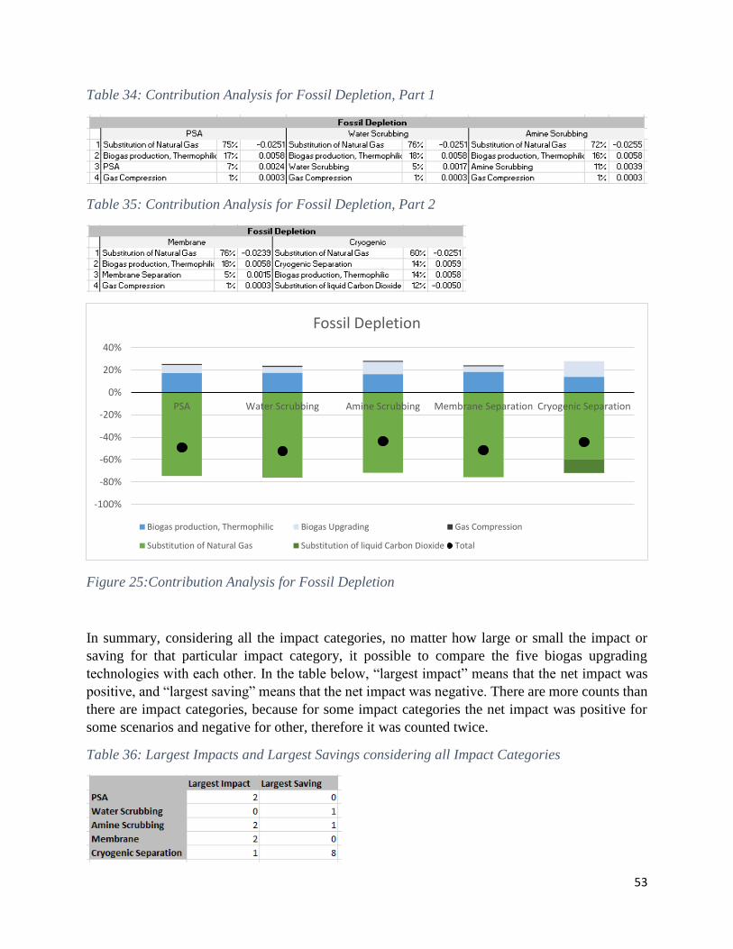
53

Table 34: Contribution Analysis for Fossil Depletion, Part 1

Table 35: Contribution Analysis for Fossil Depletion, Part 2

Figure 25:Contribution Analysis for Fossil Depletion

In summary, considering all the impact categories, no matter how large or small the impact or

saving for that particular impact category, it possible to compare the five biogas upgrading

technologies with each other. In the table below, “largest impact” means that the net impact was

positive, and “largest saving” means that the net impact was negative. There are more counts than

there are impact categories, because for some impact categories the net impact was positive for

some scenarios and negative for other, therefore it was counted twice.

Table 36: Largest Impacts and Largest Savings considering all Impact Categories

-100%

-80%

-60%

-40%

-20%

0%

20%

40%

PSA Water Scrubbing Amine Scrubbing Membrane Separation Cryogenic Separation

Fossil Depletion

Biogas production, Thermophilic Biogas Upgrading Gas Compression

Substitution of Natural Gas Substitution of liquid Carbon Dioxide Total

54

Looking at the table above, cryogenic separation seems to be the technology with the least

environmental impact. It has the largest saving for 8 of the 14 impact categories. It also only has

the largest impact for one of the impact categories, namely for ionizing radiation. PSA and

membrane separation on the other hand seem to have the worst environmental profile with having

the largest impact in two categories (climate change and photochemical oxidant formation for

membrane separation, and freshwater eutrophication and particulate matter formation for PSA)

and do not provide the largest saving for any impact category.

It is surprising that cryogenic separation seems to be the best technology from an environmental

perspective even though it applies high pressure and very low temperatures, therefore requires the

largest amount of electricity of all the five technologies. The reason why it still has the best

environmental profile is that the carbon dioxide which is separated from the methane is in liquid

form and can thereby be further utilized. For all the other technologies, the carbon dioxide as well

as the methane which slips into the byproducts is assumed to be vented into the atmosphere.

Therefore, a great way to improve the environmental impact from these technologies would be to

collect the carbon dioxide for further use.

4.1.1. Perturbation Analysis

A perturbation analysis, or so called “one-at-a-time” sensitivity analysis, examines the influence

of individual parameters on system variables (Brunner & Rechberger, 2004). One parameter is

altered at a time and then the sensitivity ratio (SR) is calculated for this parameter. The sensitivity

ratio is calculated as shown below where ΔR is the change in result, R0 is the original result, ΔP is

the change in parameter, and P0 is the original parameter:

SR = (ΔR / R0) / (ΔP / P0)

The sensitivity analysis has been done for membrane separation because for many parameters,

such as electricity use and methane slip, there was a large spread in the available data. Therefore,

it would be interesting how a change in these data will influence the environmental profile for this

upgrading technology.

The first parameter to be analyzed is the leaking of the methane between the anaerobic digester

and the biogas upgrading unit. The default value of 2% was altered half a percent up and down to

1.5% and 2.5%. The next parameter was the electricity requirement for the membrane separation.

The default value of 0.2 kWh/Nm3 had been chosen because it lies in the overlap of two sources.

Therefore, the lowest reported value of 0.15 kWh/Nm3 (Sun et al., 2015) and the highest reported

value of 0.3 kWh/Nm3 (Bauer et al., 2013) have been tested. Then also the methane slip has been

tested. The value of 8% has been tested because it lies in the middle of the interval of 2 to 13.5%

reported by Sun et al. (2015). Therefore, 2% and 13.5% have been tested. Next, the methane purity

was tested for a high value of 99% and a low of 90% according to Niesner et al. (2013). Distribution

losses were also analyzed with half a percent up and down from the original value of 2%. Lastly,

the electricity requirements for the gas compression were tested as no data besides the default

value of 0.065 kWh/Nm3 from the EASETECH process was available. Values of 0.045 kWh/Nm3

55

and 0.085 kWh/Nm3 were analyzed. Values associated with the anaerobic digestion were not tested

here as the focus of this study is on the biogas upgrading technologies and not the anaerobic

digestion. The sensitivity analysis was conducted on the normalized impact scores and “ReCiPe

Midpoint Hierarchist World” as the LCIA method.

Table 37: Original (P0) and Changed (P1 & P2) Values for Parameters for Sensitivity Analysis

The original result is the normalized impact. Therefore, for each parameter that is changed, there

are 14 impact scores, one for each impact category. The complete tables with the original value

P0, the new values P1 and P2, the changes in the values ΔP1 and ΔP2, the original result R0, the new

results R1 and R2, the changes in the results ΔR1 and ΔR2, as well as the calculated sensitivity ratios

for each impact category for each parameter can be found in Appendix V.

To compare the different sensitivity ratios for the different parameters and different impact

categories, the concept of a normalized sensitivity ratio (NSR) was used. The normalized

sensitivity ratio is defined as the ratio between the sensitivity ratio of one parameter in one impact

category and the maximum absolute value among all the sensitivity ratios of the same impact

category (Udodi, 2016):

NSRi = SRi / max(|SRi|)

For easier interpretation of the normalized sensitivity ratios, a color code was used to show whether

a parameter showed a negligible, low, medium, high, or very high sensitivity.

Table 38: Color scale for Interpreting the Normalized Sensitivity Ratios

negligible NSR < 0.1

low 0.1 < NSR < 0.5

medium 0.5 < NSR < 0.8

high 0.8 < NSR < 0.9

very high NSR > 0.9

Electricity CH4

Leaking

Methane

Slip

Methane

Purity

Distribution

Loss

Gas

Compression

[kWh/Nm3] [%] [%] [%] [%] [kWh/Nm3]

Original

Value

(P0)

0.2 2 8 96 2 0.065

1st New

Value

(P1)

0.15 1.5 2 90 1.5 0.045

2nd New

Value

(P2)

0.3 2.5 13.5 99 2.5 0.085

56

For each impact category, there is one value which scores a normalized sensitivity ratio of 1, as

this represents the highest sensitivity ratio and is therefore the value all other sensitivity ratios were

normalized by. Only the normalized sensitivity ratios for the first new value, P1, which showed a

decrease in the original value, are shown here. The normalized sensitivity ratios for the second

new value, P2, are not shown as they are basically the same as for P1. However, they can be found

in Appendix VI.

Table 39: Normalized Sensitivity Ratios for P1 with Color Coding, Part 1

Table 40: Normalized Sensitivity Ratios for P1 with Color Coding, Part 2

The table above shows the normalized sensitivity ratios for all the impact categories, however keep

in mind that the six impact categories with the largest overall impacts or savings are climate

change, freshwater eutrophication, human toxicity, freshwater ecotoxicity, marine ecotoxicity, and

fossil depletion. The main focus of the analysis will be on these six impact categories.

Out of the 14 impact categories, the methane purity had the highest sensitivity for 10 impact

categories. Of the six impact categories with the largest overall impact, the methane purity had the

largest sensitivity in four of them, namely human toxicity, freshwater ecotoxicity, marine

ecotoxicity, and fossil depletion. These were the four categories which had the largest savings. For

human toxicity, the saving increased from -0.0135 PE to -0.0148 PE; for freshwater ecotoxicity

saving increased from -0.0882 PE to -0.0950 PE, for marine ecotoxicity the saving increased from

-0.0417 PE to -0.0451 PE, and for fossil depletion the saving increased from -0.0163 PE to -0.0173

PE. This makes it seem like decreasing the methane purity is a good idea, however there is an

important thing to keep in mind. Decreasing the methane purity of the upgraded biogas means that

more carbon dioxide will end up in the upgraded biogas. It also means that there will be a larger

amount of upgraded biogas. The increased savings mentioned before are due to the increased

substitution of natural gas. However, with a lower methane purity, the biogas will be of lower

57

quality. Some countries require a certain methane purity in order to inject it into the national gas

grid. Therefore, even though the methane purity seems to be one of the most important parameters,

this parameter cannot be varied much.

For climate change, the methane slip had the largest sensitivity ratio and therefore a normalized

sensitivity ratio of 1. By decreasing the methane slip, the impact decreased from 0.0136 PE to

0.0085 PE. The large sensitivity can be attributed to the assumption that the off-gases are vented

into the atmosphere. Therefore, if the methane slip is small, a smaller portion of methane is going

to the off-gases. As methane’s global warming potential is more than 25 times larger than that of

carbon dioxide, even a small decrease in methane in the off-gases contributes a large saving on

climate change.

Lastly, for freshwater eutrophication, the largest sensitivity was found for electricity. A decrease

in the electricity consumption of the membrane separation upgrading unit caused a decrease in

impact of freshwater eutrophication from 0.0177 PE to 0.0165 PE. The likely reason for this is that

around two thirds of the electricity in the United States comes either from coal or natural gas (U.S.

Energy Information Administration (EIA), 2017). Therefore, a reduction in the electricity

consumption will reduce emissions from coal or natural gas power plants which in turn reduces

freshwater eutrophication.

In general, it is interesting to point out, that for each impact category, there is only one parameter

which a very high sensitivity. All the other parameters show either a low or even neglectable

sensitivity. For none of the impact categories or parameters, a medium or high sensitivity was

found.

4.1.2. Uncertainty Propagation

In the results section above, it was found that cryogenic separation had the largest savings in eight

of the impact categories, and therefore one could assume that it is the preferred solution. However,

as mentioned in the data collection section, most of the data falls within a range of possible values.

Thus, an uncertainty analysis was conducted to see how the results change if a range of possible

values is used as input parameters.

For each scenario, the parameters which were uncertain, were analyzed. For the parameters, for

which there was a given interval, such as electricity consumption, a triangular distribution was

chosen with the original value as the mode, the lowest given value as the lower, and the highest

given value as the upper. For parameters for which there was no given interval but it was likely

that they would vary, a normal distribution was chosen. A normal distribution is characterized by

a mean and a standard deviation. It is assumed that 95% of the values fall within two standard

deviations of the mean. A 10% variation was used except for leaking of biogas for which larger

variation was used. The following tables show which values were tested for each scenario as well

as if a triangular or normal distribution was used. No parameters for the anaerobic digestion were

tested as the focus of this study is the biogas upgrading technologies and the biogas production is

the same for all scenarios anyway.

58

Table 41: Values Used for Uncertainty Propagation, Part 1

Table 42: Values Used for Uncertainty Propagation, Part 2

Table 43: Values Used for Uncertainty Propagation, Part 3

The Monte Carlo simulation method was used which means that EASETECH takes a random value

from the uncertainty distribution for each uncertain parameter and calculates the LCA result for

this set of values. The procedure is repeated several times (SimaPro, 2015). Here, the Monte Carlo

analysis was run using 1000 sampling points for normalized impact scores using “ReCiPe

Midpoint Hierarchist World”. The results were then analyzed for the six impact categories with

the largest impact respectively savings as identified earlier, namely climate change, freshwater

eutrophication, human toxicity, freshwater ecotoxicity, marine ecotoxicity, and fossil depletion.

Be aware that the scale for the frequency and the impact scores vary for the different impact

categories.

Climate Change

Based on the first results presented in 4.1, it looked like cryogenic separation had clearly the

smallest impact on climate change, whereas the impact from membrane separation was by far the

largest. By including uncertainty, it can be seen that cryogenic separation still has the lowest

impact which does not overlap with any of the other scenarios. Therefore, it can be said with

greater certainty that cryogenic separation has the lowest impact for climate change. Membrane

separation still has the largest impact, however there is a large spread of the possible impacts. This

is due to the fact that for many of the parameters, there was a wide range of possible values. The

59

large uncertainty can also be seen on the right figure where the uncertainty bar for membrane

separation is the largest. The large uncertainty means that membrane separation is likely to have

the largest impact, however it cannot be said with complete certainty. For example, the possible

impact scores for membrane separation overlap on the lower end with the higher end of the possible

impact scores for PSA. The other three scenarios (PSA, water scrubbing, and amine scrubbing)

have a large overlap, and it is therefore not possible to say with absolute certainty that one scenario

is better than the other.

Figure 26: Uncertainty Analysis for Climate Change

Freshwater Eutrophication

Based on the first results, it looked like PSA had the largest impact with the other four scenarios

being more or less the same. By including uncertainty, it can be seen that PSA still has the largest

impact however, there is an overlap on the lower end of the impacts for PSA with the higher end

of the impacts for water scrubbing and membrane separation. Therefore, it is likely that PSA has

the largest impact for freshwater eutrophication but it cannot be said with complete certainty. Also,

the uncertainty for cryogenic separation is very large as can be seen by the impact scores being

distributed over the whole range on the left figure and by the large error bar in the right figure.

This means that cryogenic separation could have the largest impact of all, but it could also have

the smallest, or it could be somewhere in between. Therefore, it is not possible to say with absolute

certainty which scenario is the best and which is the worst regarding freshwater eutrophication.

Another interesting point is that the uncertainty for amine scrubbing is very low which can be seen

in the left figure by the fact that the range of possible impacts is very narrow and the frequency for

each impact is large. This is also represented by the very small uncertainty bar in the right figure.

0

0.05

0.1

0.15

0.2

0.25

1.4

9E-

03

2.3

4E-

03

3.1

8E-

03

4.0

3E-

03

4.8

7E-

03

5.7

2E-

03

6.5

6E-

03

7.4

1E-

03

8.2

6E-

03

9.1

0E-

03

9.9

5E-

03

1.0

8E-

02

1.1

6E-

02

1.2

5E-

02

1.3

3E-

02

1.4

2E-

02

1.5

0E-

02

1.5

9E-

02

1.6

7E-

02

1.7

6E-

02

Freq

uen

cy

Impact [PE]

Climate Change

PSA Water Scrubbing Amine scrubbing Membrane Cryogenic

60

Figure 27: Uncertainty Analysis for Freshwater Eutrophication

Human Toxicity

For human toxicity, the first results suggested that cryogenic separation had the largest saving

among the five scenarios whereas the other four are pretty much the same. The uncertainty analysis

came to the same conclusion. Even though there is a pretty large uncertainty associated to the

impact score for cryogenic separation, the whole range of impact scores is still much less than any

of the impact scores from the other scenarios. Therefore, it can be said with a large certainty, that

cryogenic separation provides the largest savings for human toxicity among all the scenarios. The

other four scenarios all overlap and it is therefore impossible to say which one is best and which

is the worst of the four.

Figure 28: Uncertainty Analysis for Human Toxicity

00.05

0.10.15

0.20.25

0.30.35

0.4

5.4

3E-

03

6.3

9E-

03

7.3

6E-

03

8.3

2E-

03

9.2

8E-

03

1.0

2E-

02

1.1

2E-

02

1.2

2E-

02

1.3

1E-

02

1.4

1E-

02

1.5

1E-

02

1.6

0E-

02

1.7

0E-

02

1.8

0E-

02

1.8

9E-

02

1.9

9E-

02

2.0

8E-

02

2.1

8E-

02

2.2

8E-

02

2.3

7E-

02

Freq

uen

cy

Impact [PE]

Freshwater Eutrophication

PSA Water Scrubbing Amine scrubbing Membrane Cryogenic

00.05

0.10.15

0.20.25

0.30.35

0.4

-2.3

9E-

02

-2.3

3E-

02

-2.2

7E-

02

-2.2

0E-

02

-2.1

4E-

02

-2.0

8E-

02

-2.0

2E-

02

-1.9

6E-

02

-1.9

0E-

02

-1.8

4E-

02

-1.7

8E-

02

-1.7

2E-

02

-1.6

6E-

02

-1.6

0E-

02

-1.5

4E-

02

-1.4

8E-

02

-1.4

2E-

02

-1.3

5E-

02

-1.2

9E-

02

-1.2

3E-

02

Freq

uen

cy

Impact [PE]

Human Toxicity

PSA Water Scrubbing Amine scrubbing Membrane Cryogenic

61

Freshwater Ecotoxicity

In the original results amine scrubbing had the largest saving by a small margin whereas membrane

separation had the smallest saving by a bigger margin. Looking at the left figure, it can be seen

that there is a large spread for all of the scenarios. Membrane separation has a large spread on the

lower end of the spectrum, however the spread is overlapping on the higher end with the lower

end from PSA. Therefore, it is not possible to say which one is clearly better or worse. On the high

side, cryogenic separation has large spread resulting in a large uncertainty. The spread results in

possible impact scores higher than amine scrubbing. Thus, it is not possible to say which scenario

yields the most savings regarding freshwater ecotoxicity.

Figure 29: Uncertainty Analysis for Freshwater Ecotoxicity

Marine Ecotoxicity

For marine ecotoxicity, cryogenic separation had the largest savings by a large margin, whereas

the other four scenarios had more or less the same impact score. The uncertainty analysis showed

the same thing. Cryogenic separation still has the largest savings and even though there is a large

uncertainty, there is no overlap with the other scenarios. Therefore, cryogenic separation has the

largest savings among the five scenarios by a large certainty. For the other four scenarios, their

possible impact scores overlap greatly and therefore it is not possible to distinguish which one is

better than the other.

0

0.05

0.1

0.15

0.2

-1.0

1E-

01

-9.9

5E-

02

-9.8

5E-

02

-9.7

5E-

02

-9.6

5E-

02

-9.5

4E-

02

-9.4

4E-

02

-9.3

4E-

02

-9.2

4E-

02

-9.1

4E-

02

-9.0

4E-

02

-8.9

4E-

02

-8.8

3E-

02

-8.7

3E-

02

-8.6

3E-

02

-8.5

3E-

02

-8.4

3E-

02

-8.3

3E-

02

-8.2

2E-

02

-8.1

2E-

02

Freq

uen

cy

Impact [PE]

Freshwater Ecotoxicity

PSA Water Scrubbing Amine scrubbing Membrane Cryogenic

62

Figure 30: Uncertainty Analysis for Marine Ecotoxicity

Fossil Depletion

In the original results, cryogenic separation had the largest savings, followed by water scrubbing,

PSA, membrane separation, and lastly amine scrubbing. However, the impact scores of all five

scenarios were very close together. Looking at the spread of the possible impact scores in the left

figure, it can be seen that the uncertainty for cryogenic separation is very large. The values are

spread almost all over the spectrum. The spread also overlaps with possible impact scores from

water scrubbing and thus it is not possible to say which of them is clearly the best. Also on the low

side of the spectrum there is great overlap, especially between membrane separation and amine

scrubbing. Therefore, it is also not possible to say with certainty which of the five scenarios is the

worst regarding fossil depletion.

Figure 31: Uncertainty Analysis for Fossil Depletion

0

0.05

0.1

0.15

0.2

0.25

0.3

-5.7

4E-

02

-5.6

5E-

02

-5.5

5E-

02

-5.4

5E-

02

-5.3

5E-

02

-5.2

5E-

02

-5.1

5E-

02

-5.0

5E-

02

-4.9

5E-

02

-4.8

5E-

02

-4.7

6E-

02

-4.6

6E-

02

-4.5

6E-

02

-4.4

6E-

02

-4.3

6E-

02

-4.2

6E-

02

-4.1

6E-

02

-4.0

6E-

02

-3.9

6E-

02

-3.8

6E-

02

Freq

uen

cy

Impact [PE]

Marine Ecotoxicity

PSA Water Scrubbing Amine scrubbing Membrane Cryogenic

0

0.05

0.1

0.15

0.2

0.25

-2.2

6E-

02

-2.2

2E-

02

-2.1

8E-

02

-2.1

4E-

02

-2.0

9E-

02

-2.0

5E-

02

-2.0

1E-

02

-1.9

7E-

02

-1.9

2E-

02

-1.8

8E-

02

-1.8

4E-

02

-1.8

0E-

02

-1.7

6E-

02

-1.7

1E-

02

-1.6

7E-

02

-1.6

3E-

02

-1.5

9E-

02

-1.5

4E-

02

-1.5

0E-

02

-1.4

6E-

02

Freq

uen

cy

Impact [PE]

Fossil Depletion

PSA Water Scrubbing Amine scrubbing Membrane Cryogenic

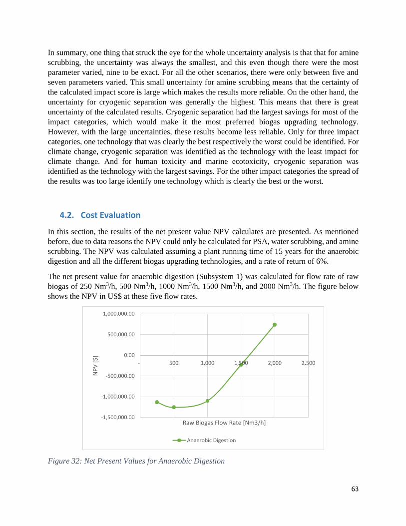
63

In summary, one thing that struck the eye for the whole uncertainty analysis is that that for amine

scrubbing, the uncertainty was always the smallest, and this even though there were the most

parameter varied, nine to be exact. For all the other scenarios, there were only between five and

seven parameters varied. This small uncertainty for amine scrubbing means that the certainty of

the calculated impact score is large which makes the results more reliable. On the other hand, the

uncertainty for cryogenic separation was generally the highest. This means that there is great

uncertainty of the calculated results. Cryogenic separation had the largest savings for most of the

impact categories, which would make it the most preferred biogas upgrading technology.

However, with the large uncertainties, these results become less reliable. Only for three impact

categories, one technology that was clearly the best respectively the worst could be identified. For

climate change, cryogenic separation was identified as the technology with the least impact for

climate change. And for human toxicity and marine ecotoxicity, cryogenic separation was

identified as the technology with the largest savings. For the other impact categories the spread of

the results was too large identify one technology which is clearly the best or the worst.

4.2. Cost Evaluation

In this section, the results of the net present value NPV calculates are presented. As mentioned

before, due to data reasons the NPV could only be calculated for PSA, water scrubbing, and amine

scrubbing. The NPV was calculated assuming a plant running time of 15 years for the anaerobic

digestion and all the different biogas upgrading technologies, and a rate of return of 6%.

The net present value for anaerobic digestion (Subsystem 1) was calculated for flow rate of raw

biogas of 250 Nm3/h, 500 Nm3/h, 1000 Nm3/h, 1500 Nm3/h, and 2000 Nm3/h. The figure below

shows the NPV in US$ at these five flow rates.

Figure 32: Net Present Values for Anaerobic Digestion

-1,500,000.00

-1,000,000.00

-500,000.00

0.00

500,000.00

1,000,000.00

- 500 1,000 1,500 2,000 2,500

NP

V [

$]

Raw Biogas Flow Rate [Nm3/h]

Anaerobic Digestion

64

Based on Figure 32, it looks like the NPV for 500 Nm3/h is lower than for 250 Nm3/h which goes

against the principle of economies of scale. Therefore, the net present value for anaerobic digestion

was divided by the raw biogas flow rate to evaluated this relationship. The NPV per flow rate now

is increasing with increasing flow rate.

Figure 33: Net Present Values per Raw Biogas Flow Rate for Anaerobic Digestion

For the second subsystem, three biogas upgrading technologies were evaluated. These

technologies are PSA, water scrubbing, and amine scrubbing. The NPV was calculated for each of

these technologies for the raw biogas flow rates of 500 Nm3/h, 1000 Nm3/h, and 2000 Nm3/h. The

following figure shows the net present values in US$ for the three flow rates. The results were

presented in the same figure for better comparison.

Figure 34: Net Present Values for Biogas Upgrading Technologies

-5,000.00

-4,000.00

-3,000.00

-2,000.00

-1,000.00

0.00

1,000.00

- 500 1,000 1,500 2,000 2,500

NP

V p

er F

low

Rat

e [$

/(N

m3

/h)]

Raw Biogas Flow Rate [Nm3/h]

Anaerobic Digestion

-2,000,000

-1,000,000

0

1,000,000

2,000,000

3,000,000

4,000,000

5,000,000

6,000,000

7,000,000

- 500 1,000 1,500 2,000 2,500

NP

V [

$]

Raw Biogas Flow Rate [Nm3/h]

PSA Water Scrubbing Amine Scrubbing

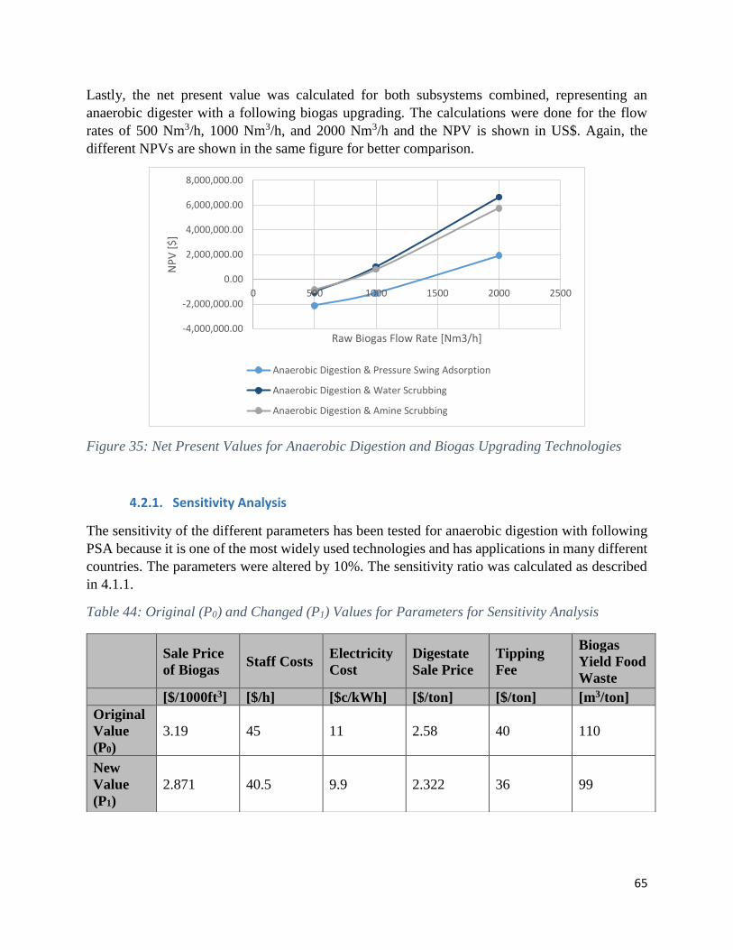
65

Lastly, the net present value was calculated for both subsystems combined, representing an

anaerobic digester with a following biogas upgrading. The calculations were done for the flow

rates of 500 Nm3/h, 1000 Nm3/h, and 2000 Nm3/h and the NPV is shown in US$. Again, the

different NPVs are shown in the same figure for better comparison.

Figure 35: Net Present Values for Anaerobic Digestion and Biogas Upgrading Technologies

4.2.1. Sensitivity Analysis

The sensitivity of the different parameters has been tested for anaerobic digestion with following

PSA because it is one of the most widely used technologies and has applications in many different

countries. The parameters were altered by 10%. The sensitivity ratio was calculated as described

in 4.1.1.

Table 44: Original (P0) and Changed (P1) Values for Parameters for Sensitivity Analysis

-4,000,000.00

-2,000,000.00

0.00

2,000,000.00

4,000,000.00

6,000,000.00

8,000,000.00

0 500 1000 1500 2000 2500

NP

V [

$]

Raw Biogas Flow Rate [Nm3/h]

Anaerobic Digestion & Pressure Swing Adsorption

Anaerobic Digestion & Water Scrubbing

Anaerobic Digestion & Amine Scrubbing

Sale Price

of Biogas Staff Costs

Electricity

Cost

Digestate

Sale Price

Tipping

Fee

Biogas

Yield Food

Waste

[$/1000ft3] [$/h] [$c/kWh] [$/ton] [$/ton] [m3/ton]

Original

Value

(P0)

3.19 45 11 2.58 40 110

New

Value

(P1)

2.871 40.5 9.9 2.322 36 99

66

The original result is the net present value for a specific flow rate. So the goal of the sensitivity

analysis is to determine the influence of each of the parameter (sale price of biogas, staff costs,

electricity cost, digestate sale price, tipping fee, and biogas yield of food waste) on the net present

value of PSA and anaerobic digestion.

P0 is the original value of the parameter as used for the calculations presented in the previous

section. ΔP is the change in the original value used for the sensitivity analysis as presented in the

table above: ΔP = original value – new value. The original value of the result R0 is the original net

present value as calculated in the previous sections (-$2,127,777 for 500Nm3/h, -$1,126,542 for

1000Nm3/h, and $1,930,477 for 2000Nm3/h). ΔR is the change in the result from changing one

parameter by 10%: ΔR = R0 – new result. The table presents the original values of the parameters

(P0), the new parameter (P1), the change in the parameters (ΔP), the original result (R0), the new

result based on the new parameter (R1) and the change in the result (ΔR). Based on these, the

sensitivity ratio can be calculated according to the equation above. The calculations were done for

the raw biogas flow ranges of 500Nm3/h, 1000Nm3/h, and 2000Nm3/h.

Table 45: Sensitivity Ratio Calculations for Pressure Swing Adsorption, Part 1

Table 46: Sensitivity Ratio Calculations for Pressure Swing Adsorption, Part 2

The sensitivity ratio calculations for the parameters for PSA showed that the tipping fee and the

biogas yield of the food waste have the largest influence on the net present value. By decreasing

the tipping fee from 40$/ton to 36$/ton, the net present value decreased by around $1.4mio for 500

Nm3/h, $2.8mio for 1000 Nm3/h, or even $5.6mio for 2000 Nm3/h. This resulted in sensitivity

ratios of -6.4 for 500 Nm3/h, -25.08 for 1000 Nm3/h, and 29.27 for 2000 Nm3/h. The reason for

the different signs of the sensitivity ratios lies in the difference in signs for R0. This however does

not impact the sensitivity analysis as the magnitude of the sensitivity ratio is most important.

Decreasing the biogas yield for food waste from 110 m3/ton to 99 m3/ton, resulted in an increase

of the net present value by $1.6mio for 500 Nm3/h, $3.3mio for 1000 Nm3/h, and almost $6.7mio

67

for 2000 Nm3/h. The reason for this increase in NPV is that due to the lower biogas yield, more

food waste is required to produce the same amount biogas, which means an increase in revenue

through tipping fees. The sensitivity ratios for the change in biogas yield from food waste were

calculated to be 7.85 for 500 Nm3/h, 29.66 for 1000 Nm3/h, and -34.62 for 2000 Nm3/h.

So in summary, the sensitivity analysis showed that the most important parameters determining

the net present value of the anaerobic digestion and the upgrading technology are the tipping fee

and the biogas yield of the food waste. As these are the most important parameters, it is important

to have reliable data for these parameters to get representative results. It is also important to note

that the tipping fee and biogas yield of the food waste only impact the NPV of the anaerobic

digester and is therefore independent of the biogas upgrading technology.

68

5. Discussion 5.1. Life Cycle Assessment

This section discusses the main findings of the LCA, the agreement of the findings with other

studies, the strength and weaknesses of this study, and the implications of the findings.

5.1.1. Main Findings

The goal of the life cycle assessment was to find the environmental impact of anaerobic digestion

and following biogas upgrading. Five different biogas upgrading technologies were evaluated such

as PSA, water scrubbing, amine scrubbing, membrane separation, and cryogenic separation.

Figure 36:Normalized Impact Scores for the Six Largest Categories with Uncertainty Bars

0

0.005

0.01

0.015

0.02

Climate Change

PSA Water Scrubbing

Amine Scrubbing Membrane Separation

Cryogenic Separation

0

0.005

0.01

0.015

0.02

0.025

Freshwater Eutrophication

PSA Water Scrubbing

Amine Scrubbing Membrane Separation

Cryogenic Separation

-0.025

-0.02

-0.015

-0.01

-0.005

0

Human Toxicity

PSA Water Scrubbing

Amine Scrubbing Membrane Separation

Cryogenic Separation

-0.1

-0.095

-0.09

-0.085

-0.08

Freshwater Ecotoxicity

PSA Water Scrubbing

Amine Scrubbing Membrane Separation

Cryogenic Separation

-0.06

-0.05

-0.04

-0.03

-0.02

-0.01

0

Marine Ecotoxicity

PSA Water Scrubbing

Amine Scrubbing Membrane Separation

Cryogenic Separation

-0.025

-0.02

-0.015

-0.01

-0.005

0

Fossil Depletion

PSA Water Scrubbing

Amine Scrubbing Membrane Separation

Cryogenic Separation

69

The two categories with the largest environmental impact were climate change and freshwater

eutrophication, and the four categories with the largest savings were human toxicity, freshwater

ecotoxicity, marine ecotoxicity, and fossil depletion. The figure above shows these six major

impact categories with the corresponding impacts for each scenario as well as the uncertainty bars.

The uncertainty analysis showed that only for three of the six categories one scenario clearly had

the smallest impact respectively the largest saving. For climate change, cryogenic separation had

the smallest impact, and for human toxicity and marine ecotoxicity, cryogenic separation had the

largest savings.

The reason for the best performance of the cryogenic separation, even though cryogenic separation

uses the largest amount of electricity among the five technologies, is because the carbon dioxide

which is separated from the raw biogas is at very high pressure and low temperature and can

therefore easily be used or stored. Thus, cryogenic separation has a second process which

contributes a saving beside the substitution of natural gas. For the other four scenarios, it was

assumed that the carbon dioxide is vented into the air which causes an impact. The environmental

impact for the other scenarios could therefore be reduced if this carbon dioxide is captured instead

of vented into the atmosphere.

For the two impact categories with the largest environmental impact, the biogas production of the

anaerobic digestion was the major contributing process for three of the scenarios for climate

change making up between 31 and 33% of the total impact, and four of the five scenarios for

freshwater eutrophication making up 74 to 76% of the total impact. Therefore, the anaerobic

digestion is the major contributor to impacts in these scenarios. In order to reduce the

environmental impact, the focus should be on reducing the impact from the biogas production.

The four impact categories with a negative impact, obviously the substitution of natural gas needs

to be the major contributor as it is the only process providing a saving (except for cryogenic

separation where the substitution of liquid carbon dioxide also provides a saving). The substitution

of natural gas makes up between 52 and 88% of the total impact across all four impact categories

and scenarios.

5.1.2. Agreement with Literature

Not many life cycle assessments have been done on the different biogas upgrading technologies.

One study on biogas upgrading technologies has been found in literature where the focus on the

removal of one ton of carbon dioxide (Starr et al., 2012).

Starr et al. (2014) has also done a life cycle assessment with the focus on global warming of eight

biogas upgrading technologies, namely high pressure water scrubbing (HPWS), amine scrubbing

(AS), organic physical scrubbing (OPS), pressure swing adsorption (PSA), membrane separation

(MS), cryogenic separation (Cry), as well as two novel upgrading technologies under development

called alkaline with regeneration (AwR) and bottom ash upgrading (BABIU) which store the

separated carbon dioxide through carbon mineralization. Whereas in this study, the functional unit

was the treatment of 1 ton of organic waste, Starr et al. (2014) used the production of 1 kWh of

70

biomethane upgraded from biogas with the composition of 50% methane and 50% carbon dioxide

as the functional unit. The system boundaries from Starr et al. (2014) were similar to this study,

however, biogas production is not considered in their study and no leaking of biogas between

processes was considered. Additionally, inventory data for Spain was used by Starr et al. (2014).

The results from Starr et al. (2014) show a saving for all categories whereas in this study all

scenarios showed an environmental impact for climate change. However, it needs to be kept in

mind that different system boundaries were used for this study compared to the study from Starr

et al. (2014). Of the five technologies used in this study, membrane separation had the lowest

saving. In this study, it was found that without uncertainty, membrane separation had the largest

impact among the five scenarios. In this study, it was also found that cryogenic separation had the

lowest impact, whereas Starr et al. (2014) found that the saving from cryogenic separation was

about the same as for water scrubbing, PSA, and amine scrubbing.

Figure 37: Global Warming Potential from Starr et al. (2014)

In summary, this shows that depending on the system boundaries, the assumptions regarding

biogas composition, and the geographical scope, the results of the life cycle assessment will be

very different.

5.1.3. Strength and Weaknesses

For this case study, a life cycle assessment was conducted using the necessary material, electricity,

heat and resulting biogas and waste products for the anaerobic digestion and the biogas upgrading

technologies. A major advantage of LCA is that all impacts over the whole life cycle of the product

are accounted for. Therefore, if reliable data is available, it contributes to consistency of the model.

The LCA shows where the environmental impacts are made and therefore shows where the largest

possibilities for impact reduction is possible. It also shows where the largest savings are regarding

certain environmental impact categories. So applying an LCA is a strength of this case study as it

shows the impacts for different categories in a consistent manner.

71

Another feature that strengthens this case study is the possibility to easily change or adjust one or

several parameters if better data is found. The EASETECH model then automatically updates all

the calculations including all the environmental impacts and presents it to the reader. This means

that the model could be used for case studies all around the world in both general or specific

contexts.

A major weakness of this study is that no data from actual plants or suppliers for the upgrading

technologies were available. This means all the calculations are based on data found in literature.

Thus, it only allows for a general analysis of the technologies but not of a specific plant in a specific

region. However, the data from literature used for the calculations is expected to be reliable and

well within the values used at actual plants. Therefore, the calculations are thought to be reliable

and accurately present a generic case for each of the upgrading technology.

Additionally, the raw biogas was assumed to only consist of methane and carbon dioxide, any

other impurities were omitted due to lack of data. In order to get a complete picture of all the

emissions, it is important to include all impurities in the raw biogas.

Another weakness of the study is that for some technologies, a wide range of data was found in

literature. For example, as mentioned in previous sections, for membrane separation the methane

slip is reported to be between 2 and 13.5%. This is a wide range and greatly affects the calculated

efficiency of the technology. As seen in the uncertainty analysis, there is a large spread of the

impact which need to be narrowed down for a more accurate study. However, even with the data

used in this study, it is still possible to get a general overview of the five investigated technologies

and to see some major advantages or disadvantages of the technology.

5.2. Cost Evaluation

This section discusses the main findings of the cost evaluation, the agreement of the findings with

other studies from literature, the strength and weaknesses of this study, and the implications of the

findings.

5.2.1. Main Findings

The goal of this part of the study was to evaluate the costs and revenues associated with an

anaerobic digester and the following biogas upgrading unit. The calculations were divided into

two subsystems, the first being the anaerobic digestion of feedstock which produces raw biogas,

and the second being five different biogas upgrading technologies to increase the methane content

of this raw biogas. The first subsystem is the same for all the different biogas upgrading

technologies. The cost evaluation was done by calculating the net present value for the anaerobic

digester as well as for the different biogas upgrading units.

The calculation for the anaerobic digestion showed that up until a plant size of around 1600 Nm3/h,

the net present value is negative, meaning that the company is losing money by investing in such

72

a project. Therefore, in order to make the project yield a profit for the investor, either a large plant

needs to build (larger than 1600 Nm3/h), or the costs need to be reduced. Looking at the investment

cost, it can be seen that the category “b) Biogas plant incl. additional building costs” makes up the

largest part of the total costs with between 42 and 46% depending on the size. Generally, for most

categories the contribution to the total cost decreases with increasing size, except for “c) substrate

storage” which increases from 18% at 250 Nm3/h to 25% at 2000 Nm3/h. Therefore, the importance

of the cost for substrate storage increase for larger plants.

Table 47: Contribution to Investment Costs for Anaerobic Digestion

Regarding the yearly cost for the anaerobic digestion, the category “a) substrate preparation (corn

silage)” makes up the largest part of these costs with between 71 to 79% depending on the size of

the plant. The plant from where the data was taken from uses corn as feedstock and therefore the

substrate needs to be prepared. Obviously, if the anaerobic digester was run using a different

substrate, there will be different costs for this. However, this also shows that by decreasing the

costs for the substrate preparation, large costs can be saved. Additionally, Besides the substrate

preparation, all category’s contribution to the total decreases with increasing plant size, except for

substrate preparation. Thus, the cost for substrate preparation becomes even more important with

increasing plant size.

Table 48: Contribution to Yearly Costs for Anaerobic Digestion

For the three biogas upgrading units, the net present value for water scrubbing and amine scrubbing

is almost the same with both being just slightly positive for a plant of 500 Nm3/h and then steadily

increasing. The slip for water scrubbing is slightly steeper meaning that at large plants, the net

present value will be larger for water scrubbing that amine scrubbing. The net present value for

PSA is negative for a plant size of 500 Nm3/h and breaks even at around 1000 Nm3/h. The NPV

then slightly increases but at a much smaller rate than water or amine scrubbing. The table below

shows a comparison for investment and yearly costs for the three biogas upgrading technologies

for different plant sizes. PSA has the highest investment cost among the three technologies and

also the highest yearly costs. This is reason for the lowest net present values for PSA. Water and

73

amine scrubbing have similar investment yearly costs, with amine scrubbing having slightly lower

investment costs but water scrubbing having lower yearly costs. This is the reason why the net

present values of these two technologies is very similar. At larger plant sizes, the yearly costs

become more important and therefore water scrubbing with the lower yearly costs has a higher net

present value than amine scrubbing. The income through the sale of biogas is pretty much the same

for all three technologies as they all treat the same amount of raw biogas and have a similar

methane slip and methane purity of the upgraded biogas.

Table 49: Comparison of Investment and Yearly Costs for Biogas Upgrading Technologies

Regarding the investment costs for the biogas upgrading plants such as PSA shown in Table 50

below, the category “a) facility including transport and installation” makes up most of the cost,

contributing between 82 and 85% of the total depending on the size. This makes sense as this is

basically the construction of the plant. It should also be noted that the contribution for the facility

is increasing with increasing plant size. The contribution is only shown here for PSA, but it is

basically the same for all the biogas upgrading units with the facility contributing the major part

of the costs.

Table 50:Contribution to Investment Cost for PSA

Table 51 shows the contribution of each category to the total yearly costs for PSA. Operating costs

contribute the majority of the costs with electricity being the major contributor to these operating

costs. The contributions for each category for the other upgrading technologies is not shown here

but they show similar values. For amine scrubbing, the majority of the operating costs is generated

not only from electricity but also from heat. Therefore, the best way to reduce the yearly cost

would be to decrease electricity (or heat) consumption.

Table 51: Contribution to Yearly Costs for PSA

74

As the electricity and heat costs are the major contributor to the yearly costs, it is interesting to

compare the electricity and heat consumption for the different upgrading technologies. The values

presented in the table below where the values used for the life cycle assessment. The table shows

that PSA uses the largest amount of electricity among the three upgrading technologies and has

therefore the largest yearly costs which in turn results in the lowest net present value.

Table 52: Electricity and Heat Requirement for Treatment of 1Nm3 of Raw Biogas

Amine

Scrubbing PSA

Water

Scrubbing

Electricity 0.13 kWh 0.31 kWh 0.22 kWh

Heat 0.55 kWh - -

Lastly, the net present value for the combination of anaerobic digestion and biogas upgrading plant

showed similar curves as for only the biogas upgrading technologies with water and amine

scrubbing being almost the same and PSA having a lower NPV for all plant sizes. This is because

the anaerobic digestion is the same for all three scenarios. Also, the income through tipping fees,

and the sale of digestate is obviously the same, but also the revenue generated by the sale of the

upgraded biogas is almost the same for all scenarios. The table below shows the contribution for

the different types of revenue to the total income. Tipping fees make up the majority of the income

with 79% followed by the sale of the upgraded biogas with 16% and the sale of digestate with 5%.

The percentage contribution is the same for all flow ranges as these incomes are calculated based

on the total flow rate. The tipping fee was also found to have the largest sensitivity ratio. Therefore,

even a small change in the tipping fee will have a large impact on the net present value.

Table 53: Contribution to Total Income for PSA

5.2.2. Agreement with Literature

The investment cost data were taken from Urban (2008). One other set of investment cost data was

found in Bauer et al. (2013) but only for the biogas upgrading technologies and not for the

anaerobic digestion. Therefore, it was not possible to compare the investment cost data. The

investment cost data in Bauer et al. (2013) were given a specific investment in €/Nm3/h for a

certain range plant sizes. The specific investment was multiplied by the flow range to get the total

investment, converted to US dollars, and adjusted for inflation assuming the data was from 2013.

The results could then be compared to the total investment from Urban (2008).

75

The investment cost for PSA are pretty much the same from both sources. Therefore, it is likely

that the data is reliable. For water scrubbing, the investment cost is similar for small plants but

then the data from Bauer et al. (2013) shows a steeper increase than from Urban (2008). For larger

plants of 2000 Nm3/h, the data from Urban (2008) predicts investment costs half of that predicted

by Bauer et al. (2013). For amine scrubbing, Bauer et al. (2013) predicts investment costs always

around half of the investment cost predicted by Urban (2008). This shows that the investment cost

is very variable and cannot be generalized. It is likely that also cost also varies depending on the

company producing and selling the upgrading plant.

Figure 38: Comparison of Investment Cost from Bauer et al. (2013) & Urban (2008)

No other data regarding yearly costs was found, therefore it is not possible to do a comparison for

the total yearly costs. However, it was mentioned before, that the electricity cost makes up the

majority of the yearly costs and electricity cost can be compared using the electricity requirement

[kWh/Nm3], the flow rate [Nm3/h], the total working hours [h/yr] and the cost of electricity

[$/kWh]. The electricity requirement was specified in data collection for the life cycle assessment,

the flow rate is give as either 500, 1000 or 2000 Nm3/h, the total working hours were specified in

data collection for cost evaluation to be 8000 h/yr, and the cost of electricity was given to be

11$cent/kWh also in data collection for cost evaluation. Multiplying all these parameters with each

other gives the cost of electricity per year [$/yr].

The calculations show that for PSA, the data from Urban (2008) and the calculated costs are very

similar. However, for water scrubbing and amine scrubbing, the calculated cost is larger than the

data given by Urban (2008). It is possible that the cost of electricity increased since the study from

Urban as the cost of electricity taken here was from this year.

76

Table 54: Comparison of Electricity Costs

5.2.3. Strength and Weaknesses

The strength and weaknesses of the cost evaluation are very similar to the ones for the life cycle

assessment. The net present value calculates allow for an easy identification of the most profitable

scenario. Also, as all calculations are connected together, it easily allows for adjustments of the

data where the model automatically calculates the new net present value. This means that input

parameters such as staff cost, electricity cost, revenue from the sale price of biogas, and such can

easily be changed and adjusted.

Again, a major weakness of the study is that no cost data from actual plants were available.

Therefore, all the calculations had to be based on literature data. Additionally, the literature data

regarding cost data for biogas upgrading technologies was were sparse. The only data that was

found was from almost 10 years ago and from Europe. Even though the data was adjusted for

inflation and converted from euros to dollars, there is still uncertainty whether any of the cost

categories have changed in recent years due to improvements in the technology or construction

and assembly. Also, comparison of the data used with other data for investment cost showed that

there is a large uncertainty in the data available. Thus, the data give a first overview of the major

cost contributors but in order to get accurate and reliable results, actual plant data need to be

available.

Another weakness of the study is that the data had to be converted from Euros to US Dollars. The

exchange rate used was taken on February 21st, 2017 at the value of 0.95 €/$. A probably better

approach would have been to take the conversion rate from 2008 as the data was from that year.

Using the average exchange rate from 2008 of 0.65 €/$ (OANDA, 2017). Using a different

conversion rate, only the values of the costs changes. The incomes stayed the same as the data for

the incomes was current. Due to the lower conversion rate, the costs in US Dollars increased

compared to the 2017 exchange rate, meaning that the investment cost and the yearly costs were

higher. The figure below shows the NPV for the anaerobic digestion and the three upgrading

technologies using a conversion rate from 2017 and from 2008.

77

Figure 39: Net Present Values for PSA, WS, and AS using 2008 and 2017 Exchange Rates

The figure shows that the net present value is negative for all upgrading technologies using the

2008 exchange rate. This is due to the higher investment cost as they increase significantly due to

the changed conversion rate. The yearly costs increase as well but as they are discounted they

become neglectable after just a few years. This shows that also the exchange rate between the

dollar and the euro has a large influence on the profitability of the different systems and therefore

this is another major weakness of this analysis.

5.3. Implication of the Findings

This case study aims to highlight the environmental impact and the costs and revenues of anaerobic

digestion and five different biogas upgrading technologies. The project has been developed in

collaboration with B&W Megtec to improve their understanding of different raw biogas upgrading

technologies.

Based on the life cycle assessment, it would appear that cryogenic separation is the

environmentally friendly technology. Cryogenic separation had clearly the lowest impact for

climate change and the largest savings from human toxicity and marine ecotoxicity. Besides the

substitution of natural gas, the carbon dioxide which is separated from the raw biogas can also be

used to substitute liquid carbon dioxide, providing another saving to the environment. For the other

four technologies, it was assumed that the carbon dioxide would be vented into the atmosphere

thus causing an impact on the environment.

However, all four technologies had very similar environmental impacts for most of the impact

categories. There was not one technology which performed considerably better or worse than the

other. The total largest normalized impact was caused by PSA for freshwater eutrophication with

0.0203 PE, and the total largest saving was achieved by amine scrubbing for freshwater ecotoxicity

with -0.0941 PE. This shows that the largest total saving was almost five times larger than the

-25,000,000.00

-20,000,000.00

-15,000,000.00

-10,000,000.00

-5,000,000.00

0.00

5,000,000.00

10,000,000.00

0 500 1000 1500 2000 2500

NP

V [

$]

Raw Biogas Flow Rate [Nm3/h]

PSA (2017 Conversion Rate) Water Scrubbing (2017 Conversion Rate)

Amine Scrubbing (2017 Conversion Rate) PSA (2008 Conversion Rate)

Water Scrubbing (2008 Conversion Rate) Amine Scrubbing (2008 Conversion Rate)

78

largest total impact. Also, in 10 of the 14 impact categories, a saving was achieved for at least one

scenario, whereas only in 7 impact categories an impact was caused in at least one category. This

shows, that overall, using either one of the biogas upgrading technologies to upgrade raw biogas

to natural gas quality provides a saving for the environment.

Amine scrubbing and water scrubbing were found to have a similarly large net present value

compared to PSA. Therefore, based on these data, it seems that either one of these two technologies

should be preferred over PSA if a profit wants to be made. Unfortunately, not enough data was

available to calculate the net present value also for membrane separation and cryogenic separation.

Therefore, no complete picture over all the five technologies is available.

The cost evaluation also showed that the construction of the facility itself is the largest part of the

investment costs. For the yearly costs, the cost for electricity was the major contributor. Therefore,

in order to reduce costs, the focus should be on reducing these major categories. For the revenues

generated, it was shown that the largest income is generated through tipping fees. However, the

tipping fees cannot be increased endlessly to increase profits, as the tipping fee at anaerobic

digesters need to be lower than the tipping fee for landfills. If this is not the case, corporations will

just deliver their organic waste to landfills instead.

In general, an important factor for choosing a technology is the methane purity of the upgraded

biogas. Often, a certain methane purity is required for the injection of the biogas into the national

gas grid. So, a technology which has a low energy consumption but produces a low calorific biogas

might not always be advantageous. If a high purity upgraded biogas is desired, cryogenic

separation should be preferred. Cryogenic separation achieves a methane purity of 98-99% and is

therefore the best technology evaluated in this regard.

Other times, it is also preferred that the methane slip be as small as possible, meaning that the

largest amount of the methane in the raw biogas ends up in the upgraded biogas. Therefore, the

loss of methane in the upgrading process should be minimized. If too much methane ends up in

the byproduct gas stream, this gas stream often needs to be torched before it can be released to the

atmosphere. Methane in the byproduct gas stream also reduces the possibilities for further use of

this gas stream. For example, if a pure carbon dioxide byproduct gas stream is produced, it can be

used in other industries such as the food processing industry. Therefore, if the goal is to reduce the

methane slip and have a byproduct gas stream with a high carbon dioxide purity, cryogenic

separation would be the preferred technology. Cryogenic separation has a methane slip reported

in literature of 0.037-1% and produces a high purity carbon dioxide stream.

In summary, the results from the life cycle impact assessment, the cost evaluation and the energy

efficiency calculations from the project work carried out in Fall 2016 show that each technology

has its own advantages and disadvantages. This is also the reason why there are so many different

technologies available. If there were one technology which would be better in all accounts, it would

not make sense to use another one. But as this is not the case, there are many different ways of

removing the carbon dioxide from the raw biogas. Also, many companies and also universities are

working on improving existing technologies or developing new technologies in order to make the

process more efficient and achieve even higher methane purities. Therefore, this case study

79

represents only an environmental and economic analysis of five respectively three biogas

upgrading technologies based on the data available now. The future might make a technology

which is preferred now undesirable, but at the same time, it might make an unrealistic technology

realistic.

80

6. Conclusions

This case study used literature data to develop a life cycle assessment for determining the

environmental impact and a cost evaluation model for determining the costs and revenues of five

different biogas upgrading technologies for biogas from anaerobic digestion: Amine scrubbing,

pressure swing adsorption, membrane separation, water scrubbing and cryogenic separation. Even

though no data from actual plants were available, it was still possible to get a general overview of

the environmental impact and economic profitability for these technologies.

The results from this case study and MFA calculations carried out as part of the project work for

Fall 2016 with the energy efficiency analysis, show that different technologies have different

advantages and disadvantages. PSA for example, is an established technology, therefore many

companies have experience and it is proven that the technology is working. Besides, there is no

waste stream such as used process water or chemicals. However, the cost evaluation showed a low

net present value. For water scrubbing, a major advantage is also that it is an established technology

with many years of experience. Besides, it had a large net present value together with amine

scrubbing. And also, the highest energy efficiency had been calculated in the project work in Fall

2016 for water scrubbing. One disadvantage however is the water usage and the need for the

treatment of this water. Amine scrubbing had a large net present value as mentioned before and is

also an established technology. However, amine scrubbing uses water and chemicals which need

to be treated before disposal. Membrane separation on the other hand uses neither water nor

chemicals, but has a large spread in the available data which makes any calculations uncertain.

Lastly, cryogenic separation had the largest savings in most of the impact categories from the life

cycle assessment. It also had the highest methane purity of the upgraded biogas and the lowest

methane slip based on literature data. Additionally, the carbon dioxide can be reused as it is of

high purity and in liquid form. However, one large disadvantage is the high energy consumption

and therefore the low energy efficiency. Besides, cryogenic separation is a newly developed

technology and only a handful of companies have experience with this technology.

Table 55: Advantages and Disadvantages of Different Biogas Upgrading Technologies

PSA Water

Scrubbing

Amine

Scrubbing

Membrane

Separation

Cryogenic

Separation

Advantage

- established

technology

- no waste

stream

- large net

present value

- established

technology

- high energy

efficiency

- large net

present value

- established

technology

- no waste

stream

- largest savings

- highest

methane purity

- carbon dioxide

can be reused

- low methane

slip

Disadvantage

- low net

present value

- water usage - water and

chemical usage

- large

uncertainty in

available data

- largest energy

consumption

- newly

developed

technology

- lowest energy

efficiency

81

In summary, this case study together with the project work from Fall 2016 give a good overview

of the environmental impact, the economic profitability, and the energy efficiency of five different

biogas upgrading technologies. The life cycle assessment showed that all five scenarios showed

very similar environmental impacts or saving for all impact categories. The economic analysis

showed that all evaluated upgrading technologies are profitable. And the material flow analysis

for the energy efficiency showed that all five technologies achieve a high energy efficiency. The

study also showed that depending on the goal of a project (high methane purity in upgraded biogas,

low energy consumption, high energy efficiency, reusable carbon dioxide stream, etc.), different

technologies are favorable.

Even though results were obtained for the life cycle assessment and the cost evaluation, these

results can only be taken as preliminary results. In order to get a comprehensive picture,

contemporary data from real plants needs to be available. Thus, the models developed as a part of

this master thesis and the project work can be taken as a starting point and then fed with realistic

data. Only if the uncertainty in the data can be kept to a minimum, the results can be taken as

realistic. Additionally, new technologies are coming to the market and these technologies should

also be taken into account and analyzed to get a complete overview of the whole market.

82

7. List of References

Angelidaki, I. (2004). The anaerobic process, 1–112.

Bauer, F., Hulteberg, C., Persson, T., & Tamm, D. (2013). Biogas upgrading – Review of

commercial technologies. Swedish Gas Technology Centre, SGC, 82. https://doi.org/SGC

Rapport 2013:270

Biogaspartner. (2011). Biogas Grid Injection in Germany and Europe - Market, Technology and

Players. Deutsche Energie-Agentur GmbH (Dena).

Börjsson, P. (2008). Biogas from waste materials as transportation fuel-benefits from an

environmental point of view. Water Science and Technology, 57(2), 271–275.

https://doi.org/10.2166/wst.2008.051

Brunner, P. H., & Rechberger, H. (2004). Practical Handbook of Material Flow Analysis. CRC

Press LLC, Boca Raton, Florida. https://doi.org/10.1002/pssb.201300062

CalRecycle. (2012). Project Descriptions: Digesting Urban Residuals Forum, May 30, 2012.

CalRecycle. (2016). State of Recycling in California Updated 2016, (February).

CalRecycle. (2017). Organic Materials Management. Retrieved May 9, 2017, from

http://www.calrecycle.ca.gov/Organics/

Chiu, S. L. H., & Lo, I. M. C. (2016). Reviewing the anaerobic digestion and co-digestion

process of food waste from the perspectives on biogas production performance and

environmental impacts. Environmental Science and Pollution Research, 1–16.

https://doi.org/10.1007/s11356-016-7159-2

Costa, A. ., Ely, C. ., Pennington, M. ., Rock, S. ., Staniec, C., & Turgeon, J. (2015). Anaerobic

Digestion and its Applications. United States Environmental Protection Agency, (October),

15.

Council Directive. (1999). Council Directive 1999/31/EC on the landfill. Official Journal of the

European Communities, (10), L182/1-19. https://doi.org/10.1039/ap9842100196

Damgaard, A., Baumeister, H., Astrup, T. F., & Christensen, T. H. (2016). EASETECH 2016.

DTU. (2017). Easetech. Retrieved April 27, 2017, from http://www.easetech.dk/

Ecoinvent. (2017). ecoinvent - the world’s most consistent &amp; transparent life cycle

inventory database. Retrieved April 11, 2017, from http://www.ecoinvent.org/home.html

Hashøj Biogas. (2017). Hashøj Biogas DK. Retrieved from http://www.hashoejbiogas.dk/#

Hauschild, M. (2015a). Chapter 9 : Introduction to the LCA methodology.

Hauschild, M. (2015b). Environmental impacts, classification and characterisation Elements of

LCA.

Hauschild, M. Z., & Barlaz, M. A. (2011). 3.1 LCA of Waste Management Systems LCA in

Waste Management : Introduction to Principle and Method. Solid Waste Technology &

83

Management, 25. https://doi.org/10.1002/9780470666883.ch10

InvestingAnswers. (2017). Net Present Value (NPV). Retrieved April 26, 2017, from

http://www.investinganswers.com/financial-dictionary/technical-analysis/net-present-value-

npv-2995

JRC European Commission. (2010). General guide for Life Cycle Assessment - Detailed

guidance. International Reference Life Cycle Data System (ILCD) Handbook.

https://doi.org/10.2788/38479

Linville, J. L., Shen, Y., Wu, M. M., & Urgun-Demirtas, M. (2015). Current State of Anaerobic

Digestion of Organic Wastes in North America. Current Sustainable/Renewable Energy

Reports, 136–144. https://doi.org/10.1007/s40518-015-0039-4

McAfee, R. P., Lewis, T., & Dale, D. J. (2006). Introduction to Economic Analysis.

Møller, J., Boldrin, A., & Christensen, T. H. (2009). Anaerobic digestion and digestate use:

accounting of greenhouse gases and global warming contribution. Waste Management &

Research : The Journal of the International Solid Wastes and Public Cleansing Association,

ISWA, 27(8), 813–824. https://doi.org/10.1177/0734242X09344876

Nakatani, J. (2014). Life cycle inventory analysis of recycling: Mathematical and graphical

frameworks. Sustainability (Switzerland), 6(9), 6158–6169.

https://doi.org/10.3390/su6096158

Naroznova, I., Møller, J., Larsen, B., & Scheutz, C. (2016). Evaluation of a new pulping

technology for pre-treating source-separated organic household waste prior to anaerobic

digestion. Waste Management, 50, 65–74. https://doi.org/10.1016/j.wasman.2016.01.042

Niesner, J., Jecha, D., & Stehlík, P. (2013). Biogas upgrading technologies: State of art review in

european region. Chemical Engineering Transactions, 35, 517–522.

https://doi.org/10.3303/CET1335086

Norz, G. (2017). Personal Communication with Megtec.

OANDA. (2017). Average Exchange Rates. Retrieved May 30, 2017, from

https://www.oanda.com/currency/average

Petersson, A., & Wellinger, A. (2009). Biogas upgrading technologies–developments and

innovations. IEA Bioenergy, 20. Retrieved from

http://typo3.dena.de/fileadmin/biogas/Downloads/Studien/IEA-

BiogasUpgradingTechnologies2009.pdf

Renewable Waste Intelligence. (2013). Business Analysis of Anaerobic Digestion in the USA,

(March).

Ryckebosch, E., Drouillon, M., & Vervaeren, H. (2011). Techniques for transformation of biogas

to biomethane. Biomass and Bioenergy, 35(5), 1633–1645.

https://doi.org/10.1016/j.biombioe.2011.02.033

SEAI sustainable energy authority of ireland. (2017). Gas Yields Table. Retrieved from

http://www.seai.ie/Renewables/Bioenergy/Bioenergy_Technologies/Anaerobic_Digestion/T

84

he_Process_and_Techniques_of_Anaerobic_Digestion/Gas_Yields_Table.pdf

Shen, Y., Linville, J. L., Urgun-Demirtas, M., Mintz, M. M., & Snyder, S. W. (2015). An

overview of biogas production and utilization at full-scale wastewater treatment plants

(WWTPs) in the United States: Challenges and opportunities towards energy-neutral

WWTPs. Renewable and Sustainable Energy Reviews, 50, 346–362.

https://doi.org/10.1016/j.rser.2015.04.129

SimaPro. (2015). Behind the Scenes at Monte Carlo Simulations - SimaPro. Retrieved June 4,

2017, from https://simapro.com/2015/behind-the-scenes-at-monte-carlo-simulations/

Starr, K., Gabarrell, X., Villalba, G., Talens, L., & Lombardi, L. (2012). Life cycle assessment of

biogas upgrading technologies. Waste Management, 32(5), 991–999.

https://doi.org/10.1016/j.wasman.2011.12.016

Starr, K., Gabarrell, X., Villalba, G., Talens Peiro, L., & Lombardi, L. (2014). Potential CO2

savings through biomethane generation from municipal waste biogas. Biomass and

Bioenergy, 62, 8–16. https://doi.org/10.1016/j.biombioe.2014.01.023

Sun, Q., Li, H., Yan, J., Liu, L., Yu, Z., & Yu, X. (2015). Selection of appropriate biogas

upgrading technology-a review of biogas cleaning, upgrading and utilisation. Renewable

and Sustainable Energy Reviews, 51, 521–532. https://doi.org/10.1016/j.rser.2015.06.029

The Engineering ToolBox. (2017). Gases - Density. Retrieved June 16, 2017, from

http://www.engineeringtoolbox.com/gas-density-d_158.html

U.S. Energy Information Administration (EIA). (2017). Frequently Asked Questions. Retrieved

June 4, 2017, from https://www.eia.gov/tools/faqs/faq.php?id=427&t=3

Udodi, O. A. (2016). Life Cycle Assessment of Mining an Old Danish Landfill. Master Thesis as

DTU.

Urban, W. (2008). Technologien und Kosten der Biogasaufbereitung und Einspeisung in das

Erdgasnetz . Ergebnisse der Markterhebung 2007-2008, 1–121.

US EPA. (2016). Program Overview for Renewable Fuel Standard Program. Retrieved

December 1, 2016, from https://www.epa.gov/renewable-fuel-standard-program/program-

overview-renewable-fuel-standard-program

Weatherbase. (2017). United States of America Travel Weather Averages (Weatherbase).

Retrieved March 27, 2017, from http://www.weatherbase.com/weather/state.php3?c=US

Wikipedia. (2017). Carbon Dioxide. Retrieved from

https://en.wikipedia.org/wiki/Carbon_dioxide

Xu, Y., Huang, Y., Wu, B., Zhang, X., & Zhang, S. (2015). Biogas upgrading technologies:

Energetic analysis and environmental impact assessment. Chinese Journal of Chemical

Engineering, 23(1), 247–254. https://doi.org/10.1016/j.cjche.2014.09.048

Yang, L., Ge, X., Wan, C., Yu, F., & Li, Y. (2014). Progress and perspectives in converting

biogas to transportation fuels. Renewable and Sustainable Energy Reviews, 40, 1133–1152.

https://doi.org/10.1016/j.rser.2014.08.008

85

86

Appendix I: Master Thesis Assignment Text

87

88

89

Appendix II: CO2 Transfer in Biogas Upgrading

For the biogas upgrading technologies, only the methane slip (the methane ending up in the carbon

dioxide stream) and the methane purity of the upgraded biogas are given. Therefore, the carbon

dioxide slip (the carbon dioxide ending up in the upgraded biogas) needs to be calculated.

Given:

- p: methane purity of upgraded biogas

- m: methane slip

Unknown:

- z: carbon dioxide slip

- x: total volume of raw biogas (will cancel out in the equation)

- a: volume of carbon dioxide in upgraded biogas (will cancel out in equation)

The raw biogas composition is given with 65% methane and 35% carbon dioxide. Assuming that

the total volume of the raw biogas is x, then the volume of the methane is 0.65x and the volume

of carbon dioxide is 0.35x. This raw biogas is split into the upgraded biogas stream with given

methane composition and a waste. The methane slip is given with m%, therefore also the volume

of methane going to upgraded biogas is (100-m)% or 0.65x*(100-m)/100. The methane purity of

the upgraded biogas, or p, is also given. Therefore, volume of methane in the upgraded biogas

previously defined is p% of the volume of the upgraded biogas. So the volume of upgraded biogas

can be defined as (0.65x*(100-m)/100)*(100/p).

Figure 40: Flowchart of Methane and Carbon Dioxide during Anaerobic Digestion

Raw Biogas

0.65x CH4

0.35x CO2

Upgraded Biogas

p% CH4

(100-p)% CO2

Byproducts

CH4

CO2

= 0.65x*(100-m)/100

= a (0.65x*(100-m)/100)*(100/p)

90

The volume of carbon dioxide in the upgraded biogas, defined as a, is therefore the difference

between the volume of the upgraded biogas minus the volume of methane in the upgraded biogas:

a = volume of upgraded biogas – volume of methane in upgraded biogas

= (0.65x*(100-m)/100)*(100/p) – 0.65x*(100-m)/100

The volume of carbon dioxide in the upgraded biogas can also be defined as the carbon slip times

the volume of carbon dioxide in the raw biogas:

a = volume of carbon dioxide in raw biogas * carbon slip

= 0.35x * (z/100)

The two equations both defining the volume of carbon dioxide in the upgraded biogas can therefore

be set equal:

(0.65x*(100-m)/100)*(100/p) – 0.65x*(100-m)/100 = 0.35x * (z/100)

or (0.65𝑥 ∗ 100−𝑚

100∗

100

𝑝 ) − 0.65𝑥 ∗

100−𝑚

100= 0.35𝑥 ∗

𝑧

100

In the first step, factor out (0.65x * (100-m)/100) on the left side:

(0.65𝑥 ∗ 100−𝑚

100) ∗ (

100

𝑝 − 1) = 0.35𝑥 ∗

𝑧

100

In the next step, the x and the divisor 100 can be canceled out as they appear on both sides of the

equation:

(0.65𝑥 ∗ 100−𝑚

100) ∗ (

100

𝑝 − 1) = 0.35𝑥 ∗

𝑧

100

(0.65 ∗ (100 − 𝑚)) ∗ (100

𝑝 − 1) = 0.35 ∗ 𝑧

Now the equation can be solved for z by dividing both sides with 0.35:

z = (0.65

0.35∗ (100 − 𝑚)) ∗ (

100

𝑝 − 1)

With this formula, the carbon dioxide slip can be calculated if the methane slip, m, and the

methane purity of the upgraded biogas, p, are given.

91

Appendix III: List of Geographies from Ecoinvent

The following table shows the names and the shortcuts of the different geographies from Ecoinvent

used in this thesis. As the geographical scope was the United States of America, the goal was to

use processes that best reflect this scope.

Table 56: List of Geographies used (Ecoinvent, 2017)

Shortcut Name

CA-QC Canada-Québec

GLO Global

RoW Rest-of-World

US United States

WECC, US only Western Electricity Coordinating Council, US part only

Remarks (Ecoinvent, 2017):

GLO: represents activities which are considered to be an average valid for all countries in this world

RoW: is generated as an exact copy of the GLO dataset with uncertainty adjustments.

92

Appendix IV: EASETECH Screenshots

Pre

ssure

Sw

ing A

dso

rpti

on

Wat

er S

crubbin

g

93

Am

ine

Scr

ubbin

g

Mem

bra

ne

Sep

arat

ion

94

C

ryogen

ic S

epar

atio

n

95

Appendix V: Sensitivity Ratio Calculations for LCA

96

97

98

Appendix VI: Normalized Sensitivity Ratios for P2

99

Appendix VII: Results from NPV calculations

These data were already presented in section 0 as figures. These just show the exact number for

the net present value which was calculated.

Table 57: Net Present Values for Anaerobic Digestion (Subsystem 1)

Table 58: Net Present Values for Biogas Upgrading Technologies (Subsystem 2)

Table 59: Net Present Values for AD & Biogas Upgrading Technologies