Costs and benefits of reducing non-point pollution from farming

Nick Hanley

Economics Department

University of Stirling, Scotland

outline

• Policy context – Water Framework Directive, Nitrates Directive

• Estimating costs of pollution control: focus on transferability of policy option rankings between two catchments

• Estimating benefits of pollution control: uses choice experiment method, and again looks at transferability of benefit estimates between the two catchments.

The WFD

The Water Framework Directive (2000/60) contains a number of ambitious aims for the future of water resource management in the EU. These include:

• protecting and enhancing aquatic ecosystems and wetlands

• promoting the sustainable long-term use of water resources

• progressively reducing emissions to the water environment

• putting incentives in place to encourage users to use water resources efficiently; and

• contributing to the mitigation of flooding and droughts.

Several key principles underlie these aims in the Directive, including implementation of the polluter pays principle, management of rivers on a river basin basis, and the setting up of cost-effective plans to achieve Good Ecological Status (GES) in all EU waters (except for cases of “disproportionate costs”).

The Water Framework Directive requires Member States to put in place Programmes of Measures (PoMs), made operational through the implementation of three iterations of River Basin Management Plans starting in 2009 and ending in 2027. The Directive requires Member States to select measures on the basis of environmental, economic and social criteria, with the aim of achieving the most cost-effective combination of measures…..

And then assessing their costs and benefits to determine and justify exemptions.

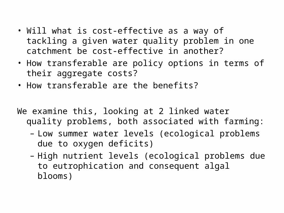
• Will what is cost-effective as a way of tackling a given water quality problem in one catchment be cost-effective in another?

• How transferable are policy options in terms of their aggregate costs?

• How transferable are the benefits?

We examine this, looking at 2 linked water quality problems, both associated with farming:– Low summer water levels (ecological problems due to

oxygen deficits)– High nutrient levels (ecological problems due to

eutrophication and consequent algal blooms)

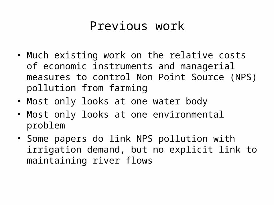
Previous work

• Much existing work on the relative costs of economic instruments and managerial measures to control Non Point Source (NPS) pollution from farming

• Most only looks at one water body• Most only looks at one environmental problem• Some papers do link NPS pollution with irrigation

demand, but no explicit link to maintaining river flows

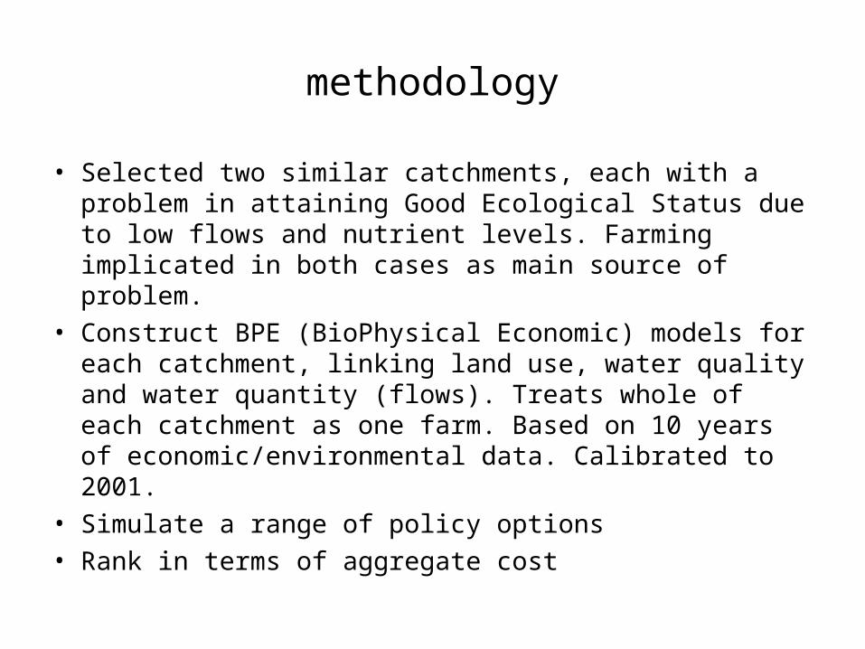
methodology

• Selected two similar catchments, each with a problem in attaining Good Ecological Status due to low flows and nutrient levels. Farming implicated in both cases as main source of problem.

• Construct BPE (BioPhysical Economic) models for each catchment, linking land use, water quality and water quantity (flows). Treats whole of each catchment as one farm. Based on 10 years of economic/environmental data. Calibrated to 2001.

• Simulate a range of policy options• Rank in terms of aggregate cost

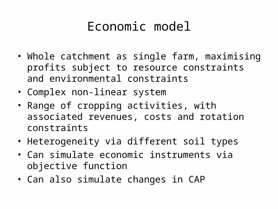
Economic model

• Whole catchment as single farm, maximising profits subject to resource constraints and environmental constraints

• Complex non-linear system• Range of cropping activities, with associated revenues,

costs and rotation constraints• Heterogeneity via different soil types• Can simulate economic instruments via objective

function• Can also simulate changes in CAP

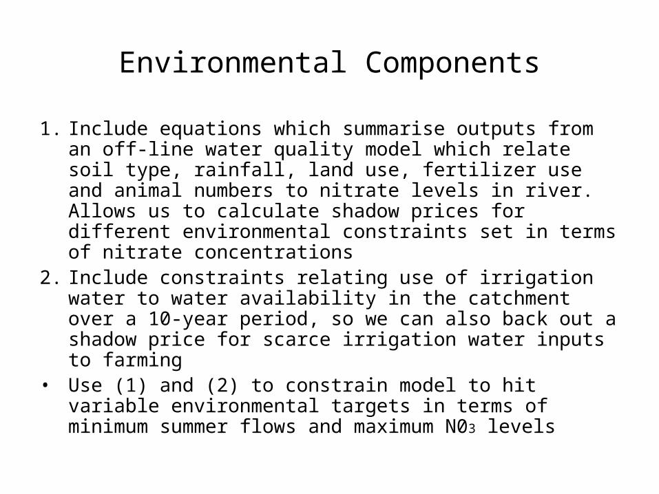
Environmental Components

1. Include equations which summarise outputs from an off-line water quality model which relate soil type, rainfall, land use, fertilizer use and animal numbers to nitrate levels in river. Allows us to calculate shadow prices for different environmental constraints set in terms of nitrate concentrations

2. Include constraints relating use of irrigation water to water availability in the catchment over a 10-year period, so we can also back out a shadow price for scarce irrigation water inputs to farming

• Use (1) and (2) to constrain model to hit variable environmental targets in terms of minimum summer flows and maximum N03 levels

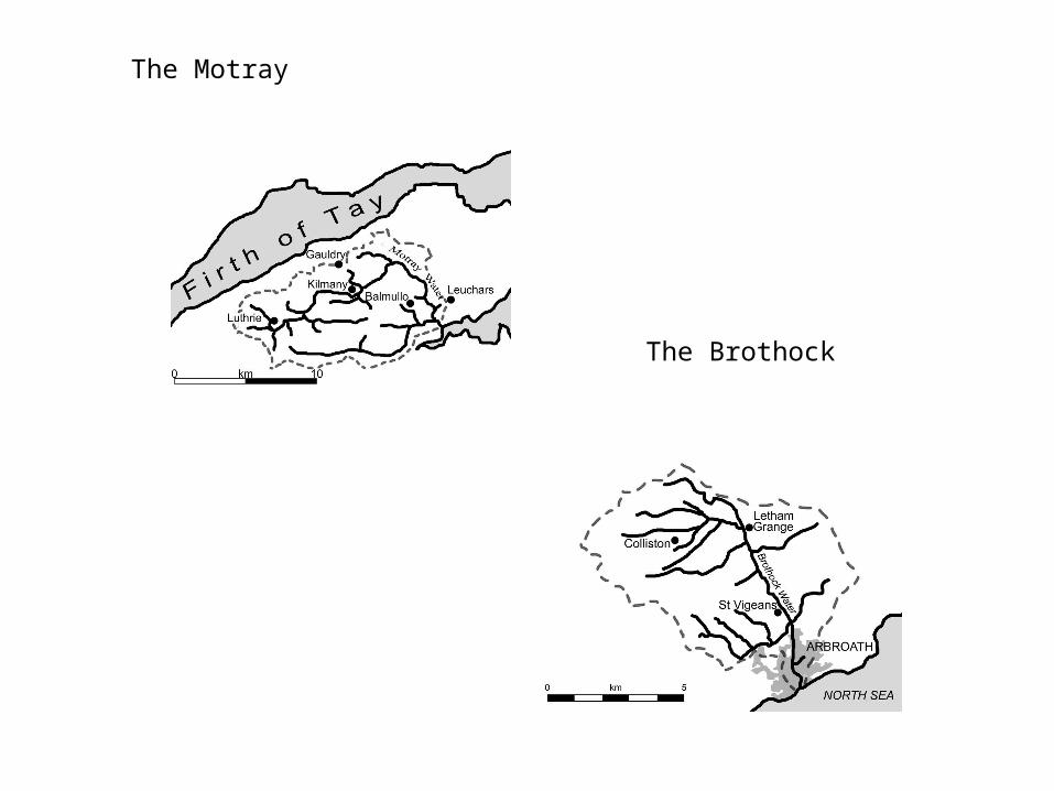
The Motray

The Brothock

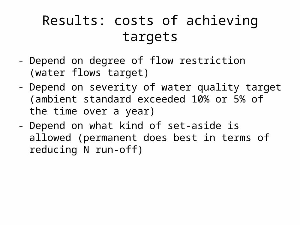
Results: costs of achieving targets

- Depend on degree of flow restriction (water flows target)- Depend on severity of water quality target (ambient

standard exceeded 10% or 5% of the time over a year)- Depend on what kind of set-aside is allowed (permanent

does best in terms of reducing N run-off)

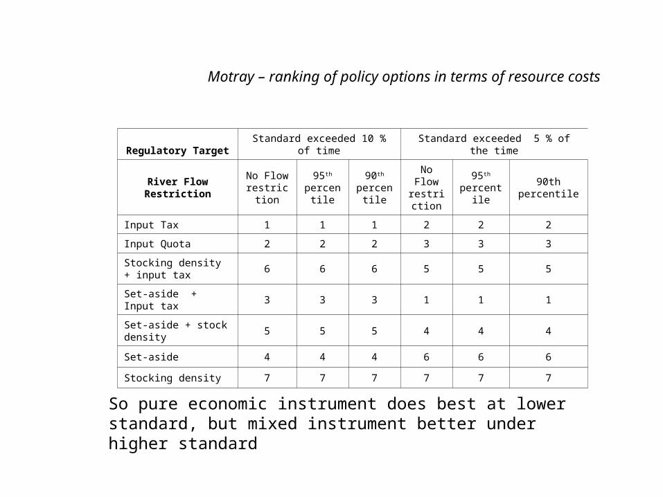
Motray – ranking of policy options in terms of resource costs

Regulatory TargetStandard exceeded 10 % of time Standard exceeded 5 % of the time

River Flow RestrictionNo Flow

restriction

95th percentil

e

90th percentil

e

No Flow restrictio

n

95th percentile

90th percentile

Input Tax 1 1 1 2 2 2

Input Quota 2 2 2 3 3 3

Stocking density + input tax

6 6 6 5 5 5

Set-aside + Input tax 3 3 3 1 1 1

Set-aside + stock density 5 5 5 4 4 4

Set-aside 4 4 4 6 6 6

Stocking density 7 7 7 7 7 7

So pure economic instrument does best at lower standard, but mixed instrument better under higher standard

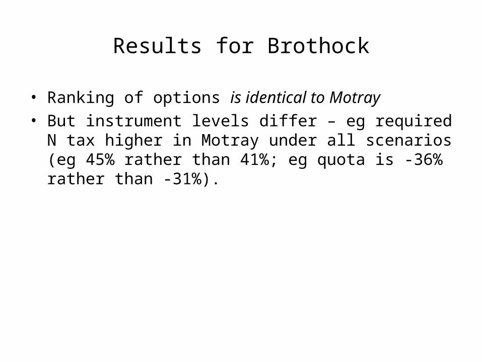
Results for Brothock

• Ranking of options is identical to Motray• But instrument levels differ – eg required N tax higher in

Motray under all scenarios (eg 45% rather than 41%; eg quota is -36% rather than -31%).

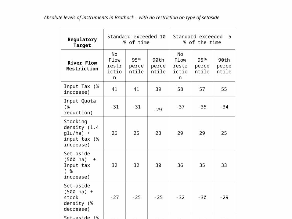
Absolute levels of instruments in Brothock – with no restriction on type of setaside

Regulatory Target

Standard exceeded 10 % of time

Standard exceeded 5 % of the time

River Flow Restriction

No Flow restriction

95th percentile

90th percentile

No Flow restriction

95th percentile

90th percentile

Input Tax (% increase)

41 41 39 58 57 55

Input Quota (% reduction)

-31 -31 -29

-37 -35 -34

Stocking density (1.4 glu/ha) + input tax (% increase)

26 25 23 29 29 25

Set-aside (500 ha) + Input tax ( % increase)

32 32 30 36 35 33

Set-aside (500 ha) + stock density (% decrease)

-27 -25 -25 -32 -30 -29

Set-aside (% increase)

292 287 280 365 352 320

Stocking density (% decrease)

-40 -39 -37 -51 -51 -49

Conclusions on costs

• Costs depend on severity of target, and whether aiming for joint targets (flows and quality).

• Economic instruments typically cost-effective, but under some circumstances (higher quality target) a MIX of economic instruments and regulation is most cost-effective.

• Note that we do not model changes in the price of irrigation – farmers in Scotland currently pay no fee for water use.

• Optimal input tax varies across catchments• But ranking of policy options is the same

Estimating the benefits of improvements in water flows and water quality

• Focus on same two catchments• Focus on same water quality and flow issues• Question: can we transfer the benefit values between

these catchments?• This is interesting because, under the WFD,

environmental agencies will have to undertake a great many benefit transfer exercises to decide which improvements to Good Ecological Status are “dis-proportionately costly”

• We use a Choice Experiment to do this. • Hanley et al, Euro. Rev. Ag. Econ., 2006.

Choice Experiments (CE)

• Based on characteristics theory of value and random utility theory

• Assumes utility function can be de-composed into deterministic and random components

• Train (1998) introduced the Random Parameter version of the model, which “improves” on the more usual conditional logit by allowing for preference heterogeneity: estimate both a mean effect of an attribute on choice and the standard deviation of this effect. Also allows for correlation across choices by an individual

• Standard RPL assumes attributes are uncorrelated. We relax this : people who like attribute “a” more might also like attribute “b” more.

RPL – basic specification

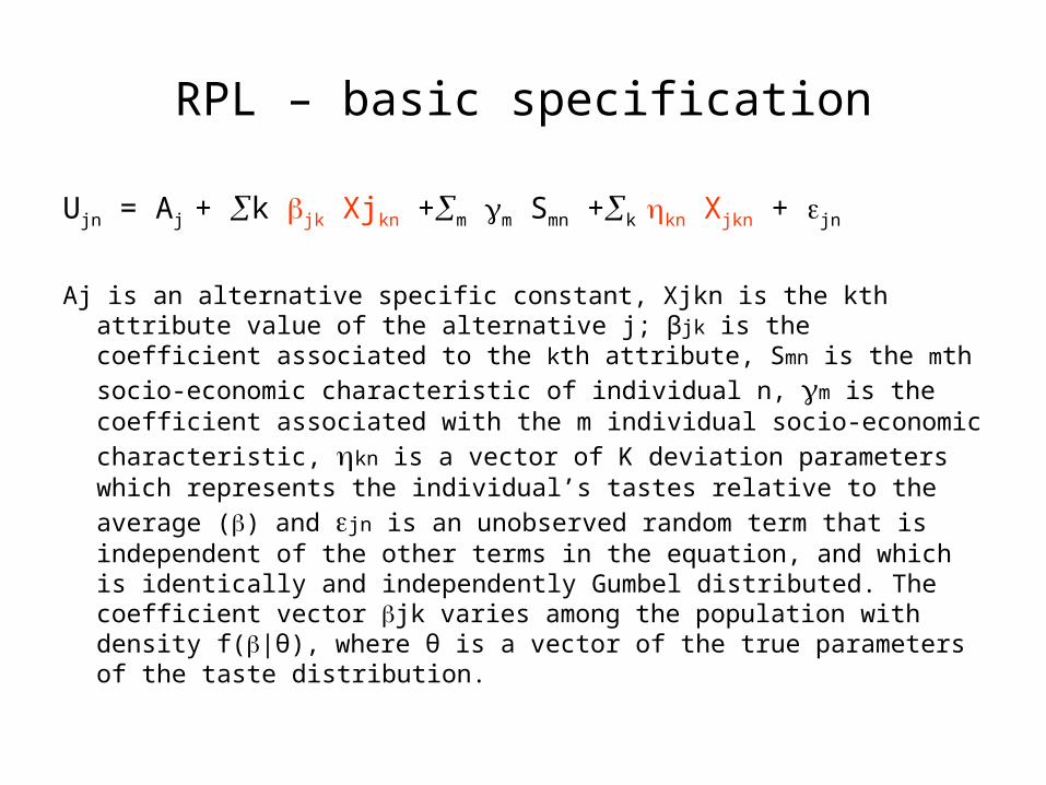
Ujn = Aj + k jk Xjkn +m m Smn +k kn Xjkn + jn

Aj is an alternative specific constant, Xjkn is the kth attribute value of the alternative j; βjk is the coefficient associated to the kth attribute,

Smn is the mth socio-economic characteristic of individual n, m is the coefficient associated with the m individual socio-economic

characteristic, kn is a vector of K deviation parameters which

represents the individual’s tastes relative to the average () and jn is an unobserved random term that is independent of the other terms in the equation, and which is identically and independently Gumbel distributed. The coefficient vector jk varies among the population with density f(|θ), where θ is a vector of the true parameters of the taste distribution.

Steps in CE design

• Choose attributes and levels• Design choice sets• Choose population to sample• First two are based on some likely “policy scenarios”, described in

terms of changes in abstraction licensing and controls on fertiliser use, and how these would impact on the appearance and ecological quality of the river

• Levels/attributes:– Ecological condition (worse, slight improvement, big

improvement)– Flow rate (months of low flow)– Agricultural jobs– Cost of programme to local households

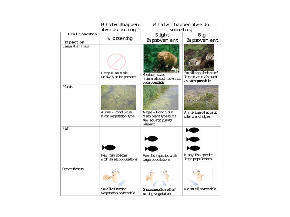
What will happen if we do nothing

What will happen if we do something

Ecol. Condition Impact on

Worsening Slight

Improvement Big

Improvement Large Mammals

Large Mammals unlikely to be present

Medium sized mammals such as water vole possible

Small populations of large mammals such as otter possible

Plants

Algae – Pond Scum main vegetation type

Algae – Pond Scum main plant type but a few aquatic plants present

A mixture of aquatic plants and algae

Fish

Few fish species with small populations

Few fish species with large populations

Many fish species large populations.

Other factors

Smell of rotting vegetation noticeable

Occasional smell of rotting vegetation

No smell noticeable

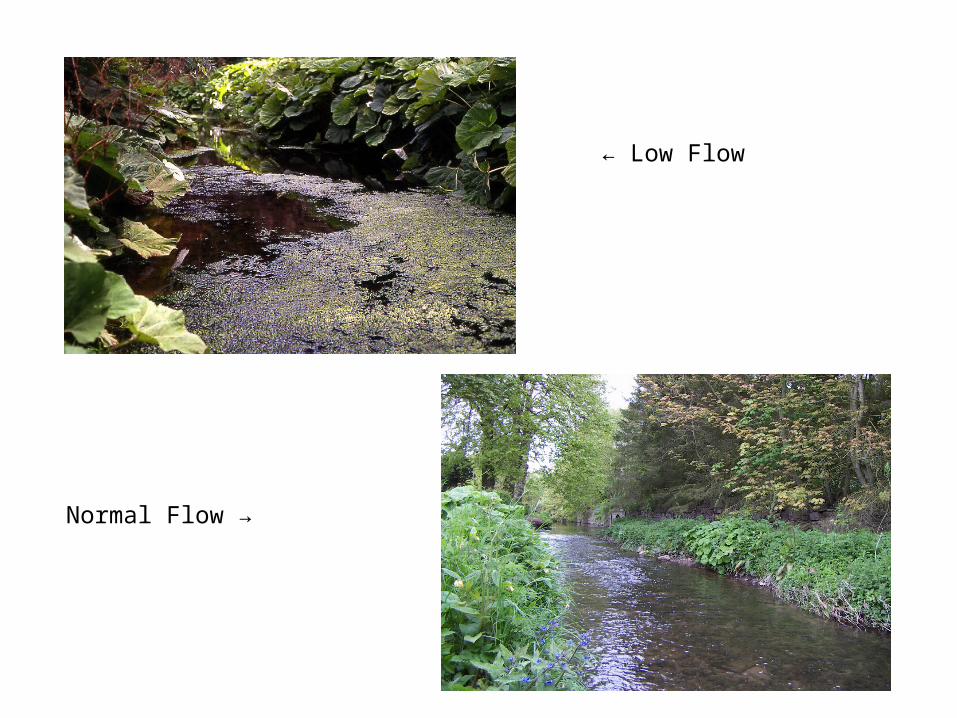
← Low Flow

Normal Flow →

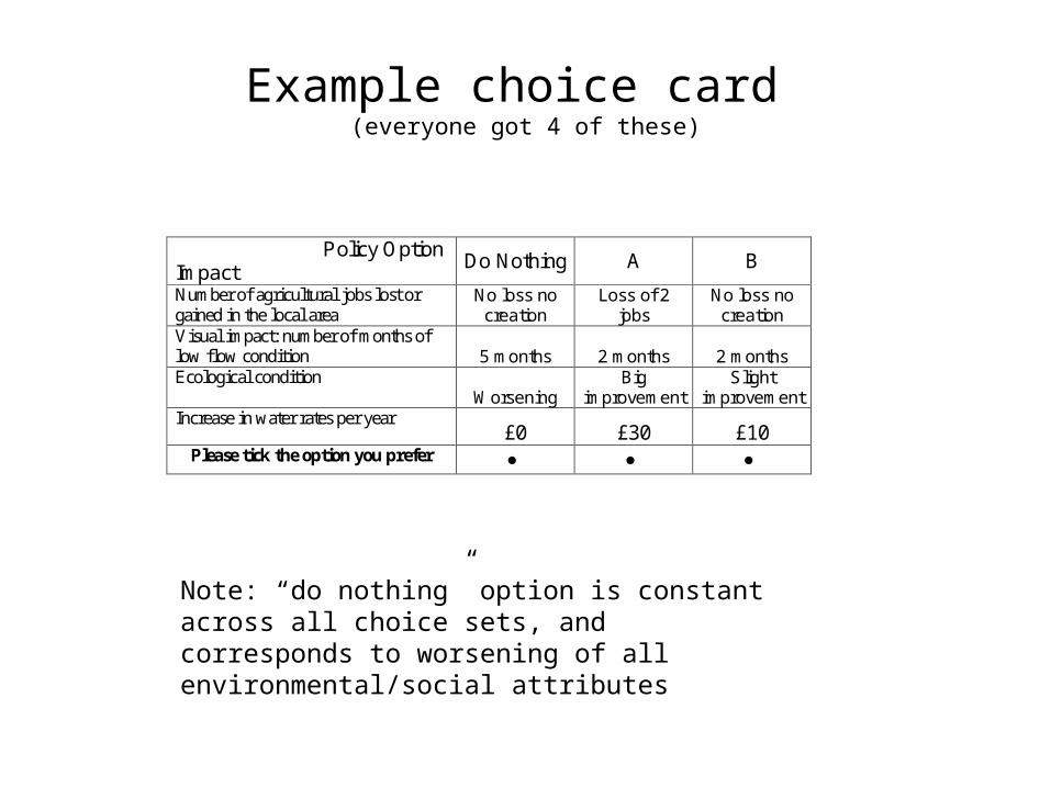
Example choice card (everyone got 4 of these)

Policy Option Impact

Do Nothing A B

Number of agricultural jobs lost or gained in the local area

No loss no creation

Loss of 2 jobs

No loss no creation

Visual impact: number of months of low flow condition 5 months 2 months 2 months Ecological condition

Worsening Big

improvement Slight

improvement Increase in water rates per year

£0 £30 £10 Please tick the option you prefer

Note: “do nothing” option is constant across all choice sets, and corresponds to worsening of all environmental/social attributes

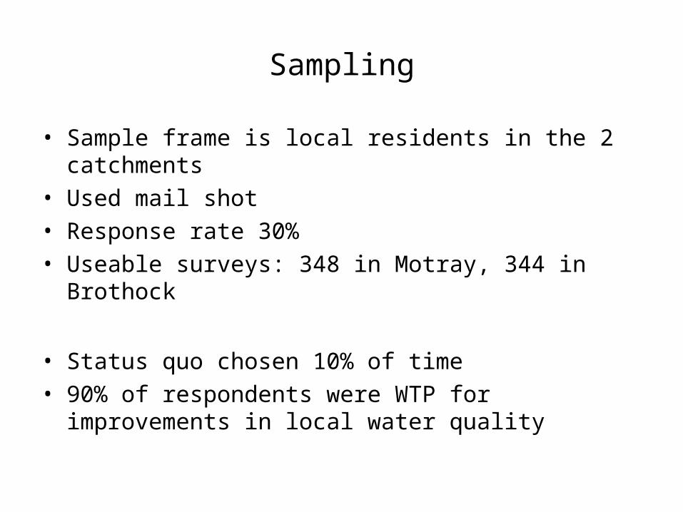
Sampling

• Sample frame is local residents in the 2 catchments• Used mail shot• Response rate 30%• Useable surveys: 348 in Motray, 344 in Brothock

• Status quo chosen 10% of time• 90% of respondents were WTP for improvements in local

water quality

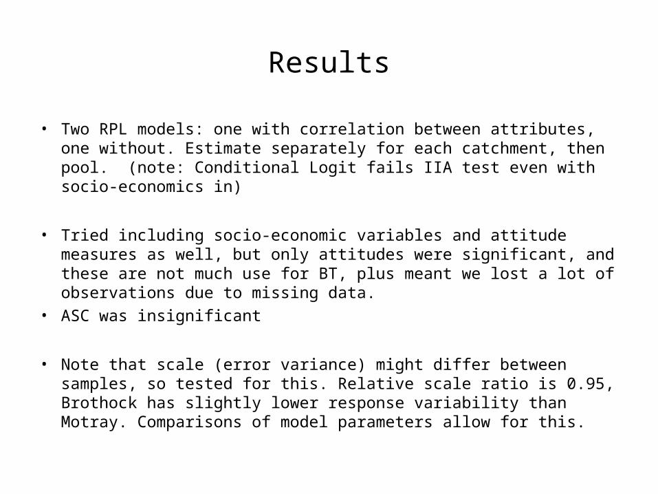
Results

• Two RPL models: one with correlation between attributes, one without. Estimate separately for each catchment, then pool. (note: Conditional Logit fails IIA test even with socio-economics in)

• Tried including socio-economic variables and attitude measures as well, but only attitudes were significant, and these are not much use for BT, plus meant we lost a lot of observations due to missing data.

• ASC was insignificant

• Note that scale (error variance) might differ between samples, so tested for this. Relative scale ratio is 0.95, Brothock has slightly lower response variability than Motray. Comparisons of model parameters allow for this.

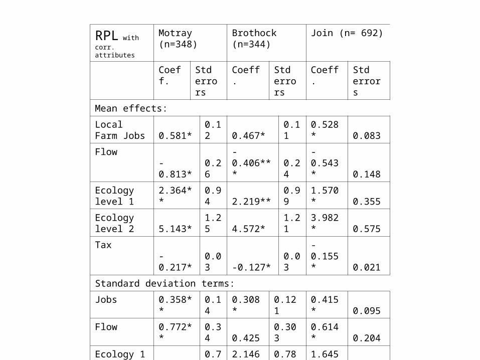
RPL with

corr. attributes

Motray (n=348) Brothock (n=344) Join (n= 692)

Coeff. Stderrors

Coeff. Stderrors

Coeff. Stderrors

Mean effects:

Local Farm Jobs 0.581* 0.12 0.467* 0.11 0.528* 0.083

Flow -0.813* 0.26 -0.406*** 0.24 -0.543* 0.148

Ecology level 1 2.364** 0.94 2.219** 0.99 1.570* 0.355

Ecology level 2 5.143* 1.25 4.572* 1.21 3.982* 0.575

Tax -0.217* 0.03 -0.127* 0.03 -0.155* 0.021

Standard deviation terms:

Jobs 0.358** 0.14 0.308* 0.121 0.415* 0.095

Flow 0.772** 0.34 0.425 0.303 0.614* 0.204

Ecology 1 2.536* 0.74 2.146* 0.782 1.645* 0.329

Ecology 2 4.334* 0.79 2.522** 1.347 2.472* 0.560

Log Likelihood (pseudo-R2)

-220.67 (0.38)

-242.76(0.34)

-467.00 (0.36)

BT tests

1. Are the models the same? Likelihood ratio test says we cannot reject the null hypothesis of parameter equality once we allow for difference in relative scale

β(Motray) = β (Brothock) ……unusual!

BT testing (2)

Are the implicit prices different? Implicit price for attribute a = βa/βcost.

Test for implicit price (low flows, Brothock) = implicit price (low flows, Motray) ,and for ecological quality, using Poe et al (1994) test. Results: depends on whether use correlated attribute version of model or not.

With correlation: no differences in implicit prices for any attributeWithout correlation: jobs and big improvement in ecology are

significantly different

Comparing the “pooled” model, which might be the benefits transfer system, with the two catchment models, also get transferable estimates with the un-correlated attributes version of the model, and signif. diff. for one attribute for each river with correlated preferences

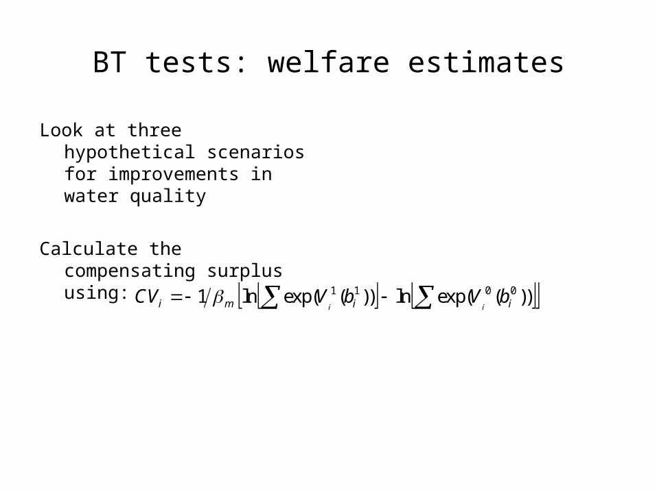
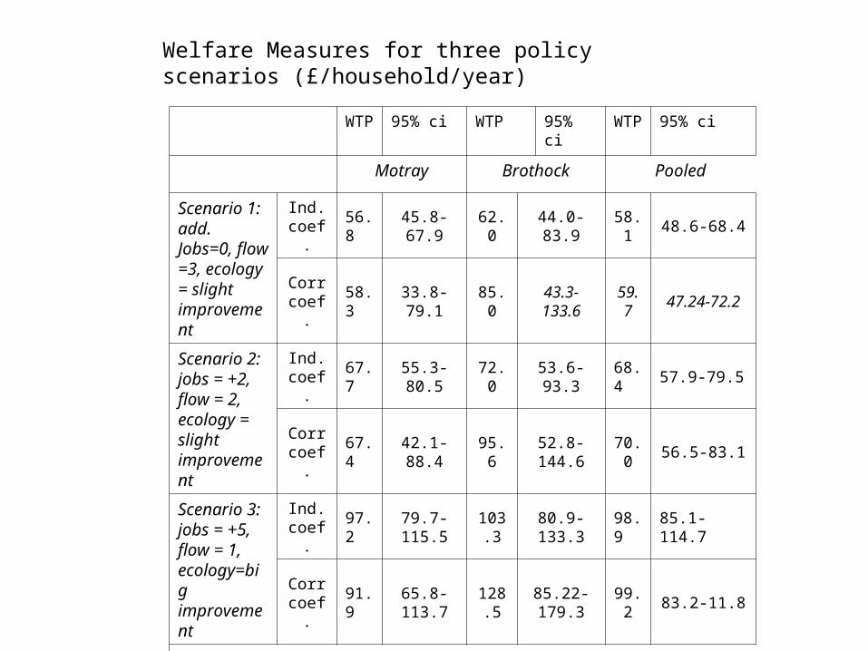
BT tests: welfare estimates

Look at three hypothetical scenarios for improvements in water quality

Calculate the compensating surplus using:

))(exp(ln))(exp(ln1 0011

iimi bVbVCVii

WTP

95% ci WTP 95% ci WTP

95% ci

Motray Brothock Pooled

Scenario 1: add. Jobs=0, flow =3, ecology = slight improvement

Ind.coef.

56.8 45.8-67.9 62.0 44.0-83.9 58.1 48.6-68.4

Corr coef.

58.3 33.8-79.1 85.0 43.3-133.6 59.7 47.24-72.2

Scenario 2: jobs = +2, flow = 2, ecology = slight improvement

Ind.coef.

67.7 55.3-80.5 72.0 53.6-93.3 68.4 57.9-79.5

Corr coef.

67.4 42.1-88.4 95.6 52.8-144.6 70.0 56.5-83.1

Scenario 3: jobs = +5, flow = 1, ecology=big improvement

Ind.coef.

97.279.7-115.5

103.3

80.9-133.3 98.9 85.1-114.7

Corr coef.

91.965.8-113.7

128.5

85.22-179.3

99.2 83.2-11.8

V0 Base: jobs = -2, flow = 5, ecology = worsening

Welfare Measures for three policy scenarios (£/household/year)

• Welfare estimates are more precise for the “without correlation” model

• Same improvements valued more highly in the Brothock than the Motray, although the difference is not significant using the Poe et al (1994) test

• Might make sense – current water quality is slightly worse in the Brothock

• But in both models, using either catchment to predict values of water quality improvement in the other would not produce significant errors – encouraging finding?

Conclusions - benefits

• Much greater need for benefits transfer now that WFD is being implemented, and river basin management plans are being drawn up

• Choice experiments offer quite a bit of flexibility as the basis of a BT system, but not much evidence to date as to their performance in this regard

• Our findings show that whether one allows for correlation between attributes seems to make a difference. Our earlier work showed that allowing for preference heterogeneity via RPL could reduce transfer errors

• So we are getting nearer an “acceptable” system? Seems to depend, in our paper, on how one tests for differences

• But what do we conclude if we accept value function and welfare estimate transfer, but reject implicit price transfer?? Depends what we want to know

• How close is “close enough” for policy purposes? 95% is probably too strict?