Embed Size (px)
Citation preview
NBER WORKING PAPER SERIES
COSTS OF AIR QUALITY REGULATION
Randy A. BeckerJ. Vernon Henderson
Working Paper 7308http://www.nber.org/papers/w7308
NATIONAL BUREAU OF ECONOMIC RESEARCH1050 Massachusetts Avenue
Cambridge, MA 02138August 1999
The authors thank the National Science Foundation for Support, as well as the National Bureau of EconomicResearch and the Fondazione Eni Enrico Mattei. This work has benefited from the comments of those at theNBER-FEEM conferences as well as seminar participants at the Center for Economic Studies (U.S. Bureauof the Census). The views expressed herein are those of the authors and not necessarily those of theNational Bureau of Economic Research or of the Bureau of the Census. All papers are screened to ensurethat they do not disclose any confidential information.
© 1999 by Randy A. Becker and J. Vernon Henderson. All rights reserved. Short sections of text, not to
exceed two paragraphs, may be quoted without explicit permission provided that full credit, including © notice,is given to the source.Costs of Air Quality RegulationRandy A. Becker and J. Vernon HendersonNBER Working Paper No. 7308August 1999
ABSTRACT
This paper explores some costs associated with environmental regulation. We focus on regulation
pertaining to ground-level ozone (O3) and its effects on two manufacturing industries -- industrial organic
chemicals (SIC 2865-9) and miscellaneous plastic products (SIC 308). Both are major emitters of volatile
organic compounds (VOC) and nitrogen oxides (Nox), the chemical precursors to ozone. Using plant-level
data from the Census Bureau’s Longitudinal Research Database (LRD), we examine the effects of
regulation on the timing and magnitudes of investments by firms and on the impact it has had on their
operating costs. As an alternative way to assess costs, we also employ plant-level data from the Pollution
Abatement Costs and Expenditures (PACE) survey.
Analyses employing average total cost functions reveal that plants’ production costs are indeed
higher in (heavily-regulated) non-attainment areas relative to (less-regulated) attainment areas. This is
particularly true for younger plants, consistent with the notion that regulation is most burdensome for new
(rather than existing) plants. Cost estimates using PACE data generally reveal lower costs. We also find
that new heavily-regulated plants start our much larger than less-regulated plants, but then do not invest as
much. Among other things, this highlights the substantial fixed costs involved in obtaining expansion permits.
We also discuss reasons why plants may restrict their size.
Randy Becker Vernon HendersonCenter for Economic Studies Department of EconomicsUS Bureau of the Census Brown University4700 Silver Hill Road, Stop 6300 Box BWashington, DC 20233-6300 Providence, RI [email protected] and NBER
Introduction
An ongoing debate in the United States concerns the costs environmental regulations
impose on industry. In this paper, we explore some of the costs associated with air quality
regulation. In particular, we focus onjegulation pertaining to ground-level ozone (03) and its
effects on two industries sensitive to such regulation — industrial organic chemicals (SIC 2865-
9) and miscellaneous plastic products (SIC 308). Both of these industries are major emitters of
volatile organic compounds (VOC) and nitrogen oxides (NOr), the chemicalprecursors to ozone.
Using plant-level data from the Census Bureau's Longitudinal Research Database (LRD), we
examine the effects this type of regulation has had on the timing and magnitudes of investments
by firms in these industries and on the impact it has had on their operating costs. As an
alternative way to assess costs, we also employ plant-level data from the Pollution Abatement
Costs and Expenditures (PACE) survey.
Our prior work has found a variety of effects on industry behavior attributable to
environmental costs (Becker and Henderson, 2000). Here we attempt to quantify some of these
costs. To identify effects, we use spatial variation in regulatory stringency as well as temporal
differences arising from the introduction of heightened regulation. Our previous research has
shown that plant age and plant size are important determinants of who gets regulated when and
how intensely, so we incorporate these elements into our analysis here as well. Our models also
control for location-specific fixed effects, which is critical in this type of work. Here, we find
that regulation indeed significantly increases production costs, especially foryoung plants, with
estimates that (arguably) are higher than what expenditure data from the PACEsurvey suggest.
Our results also show that regulation may lead plants to restrict their size, and reasons for why
this might be the case are discussed. We also find that, in at least one of these two industries,
investment profiles are significantly altered for plants subject to regulation, with relatively more
up-front investment and less phasing-in.
In the next section, we offer a general overview of air quality regulation in the United
States, introducing our key environmental variable and discussing some of the difficulties
2
involved in identifying a control and treatment group for empirical work. In the section that
follows, we discuss the results from our prior research that led us to our current focus. We then
turn to a description of our data. The three ensuing sections present results from our analyses of
the size and timing of investments, regulatory costs using data from the LRD, and cost estimates
using PACE data. The final section offers some concluding remarks.
The Nature of Air Ouality Regulation
Each year (since 1978) each county in the United States is designated as either being in or
out of attainment of the National Ambient Air Quality Standards (NAAQS's) for ground-level
ozone. Areas that are in non-attainment of this standard are, by law, required to bring
themselves into attainment, or face harsh federal sanctions. The primary way of achieving
attainment is through the regulation of VOC- and NOR-emitting sources within one's jurisdiction
— particularly manufacturing plants in certain industries. As a result, these plants in non-
attainment areas face much stricter environmental regulation than their counterparts in
attainment areas.
For example, in non-attainment areas, plants with the potential to pollute are subject to
more stringent and more costly technological requirements on their capital equipment. New
plants wanting to locate in non-attainment counties (as well as existing ones undertaking major
expansion andlor renewal) are subject to Lowest Achievable Emission Rates (LAER), requiring
the installation of the "cleanest" available equipment without regard to cost. Existing plants in
non-attainment counties, who are grandfathered from these strict requirements (at least until they
update their equipment), are required to install Reasonably Available Control Technology
(RACT), usually some simple retro-fitting, which is to take into account the economic burden it
places on a firm. In contrast, in attainment counties, only new plants only those with the
potential to emit over (originally) 100 tons per year of a criteria pollutant are subject to any
regulation on their capital equipment, and the technological standard is a weaker one. Rather
than LAER, large new plants in attainment counties are required to install Best Available Control
3
Technology (BACT), which is negotiated on a case-by-case basis and is to be sensitive to the
economic impact on a firm. Existing plants and small new plants in attainment areas face no
specific requirements on their capital equipment.
In addition to more stringent technological requirements, non-attainment status also usually
entails higher costs in other areas as well. Forced to "produce environmental quality," plants in
non-attainment areas must purchase additional inputs. Additional labor is certainly required;
however, "environmental production" may also call for more (and/or more expensive) materials
and energy as well. Costly redesigns to production processes can also be involved. Andany
proposed expansion — either the construction of a new plant or the modification of an existing
facility — must first be approved by environmental regulators. This permitting process can
involve lengthy and costly negotiations over equipment specifications, emission limits, and the
like. The purchase of pollution offsets may also be required. Finally, plants in non-attainment
areas face a greater likelihood of being inspected and fined than their counterparts in attainment
areas.
As this discussion reveals, we have (at least in principle) a control and treatment group
with which to estimate the costs of regulation. In particular, given age (i.e., new versus existing
plants), we would expect capital costs, labor costs, operating costs, and so forth to be higher for
plants in counties classified as being in non-attainment of the NAAQS for ozone, than for plants
located in counties classified as being in attainment. The reality of the situation, however, is a
bit murkier than this neat dichotomy would suggest. First, within a county, regulatory scrutiny
often varies by plant size. In attainment areas, large new plants are required to install BACT
while small new plants have no specific requirements. In non-attainment areas, differential
treatment is defacto rather than by decree. Local regulators, who are generally resource
constrained, focus their enforcement on larger (and hence more polluting) plants while smaller
plants have been slow to be classified as polluters, and once classified, may be inspected
infrequently or not at all. Then, given plant age and size, regulatory treatment of otherwise
similar polluters may differ from one non-attainment area to the next because of variation in state
4
philosophies on how best to achieve attainment. Even within a state, non-attainment areas may
face different degrees of regulation because they differ in the extent to which they are in non-
attainment. Dissimilarities between attainment areas also exist, as some face a degree of
regulation above what is normally reuired of them simply because they are in states with strong
environmental agendas.
In the empirical specifications that follow, we are mindful of differences in regulatory
treatment that are due to plant characteristics, such as age and size. The remaining differences,
then, between attainment and non-attainment areas are typical differences, alert to the fact that
each group itself may have some significant variation in regulatory intensity. We also note two
potential qualifications that affect this interpretation of our results. First, there's the notion that
plants in attainment areas may incur environmental costs "voluntarily," as opposed to being
required to do so by regulators. Such plants, for example, may be reluctant to install "dirty"
production equipment in this day and age for fear of protests and law suits, as well as inducing
active regulation. Furthermore, for plants in many industries, "dirty" equipment that may still be
permissible for use in attainment areas may no longer be available for purchase. Prior to the
regulatory era, plants in polluting industries were mostly located in (what would become) non-
attainment areas and a considerable proportion still remain there. These producers spur
technological innovation and create a market for "green" production equipment that have
affected equipment choices for everyone. Therefore, plants in attainment areas may incur
'environmental costs' that are not the result of regulation per Se, but rather are the result of
various other forces (social, political, technological, etc.). Our approach, therefore, of comparing
plants in attainment and non-attainment areas, won't reveal the full costs of regulation (gotten
from comparing a world with regulation to one without regulation and these other forces) but
should at least reveal a lower bound on the costs of regulation.
Our second qualification only serves to lower this lower bound even further. In particular,
plants may self-select themselves into attainment or non-attainment areas. For example, it may
be the case that firms who choose to locate in non-attainment areas may, to some extent, be those
5
who can best handle regulatory costs. Firms in attainment areas, on the other hand, may be ones
for whom regulation would be particularly burdensome. This would suggest that our estimates
of regulatory costs are for a select group — understating costs for the typical plant.' Both these
qualifications should be kept in mindivhen interpreting the results below.
Prior Findings and Current Motivation
In our previous work in this area (Becker and Henderson, 2000) we investigate the effects
ozone non-attainment (versus attainment) status has had on the decisions of firms in polluting
industries. In that study (described in more detail below) we focus on major VOC (and NON)
emitting industries that: (a) have had large numbers of plants and plant births (nationally), and
(b) do not have (as) much other air pollution emissions. These industries are: industrial organic
chemicals (SIC 2865-9), miscellaneous plastic products (SIC 308), metal containers (SIC 3411-
2), and wood household furniture (SIC 2511). In this current paper, we focus on just the first
two of these. Industrial organic chemicals, as in turns out, is the heaviest polluter of all of these
industries (it actually manufactures VOCs!) and has the largest average plant sizes.
Miscellaneous plastic products uses VOCs in its production and has the convenient property of
being the industry with the largest sample size. Plant-level data for both studies come from the
1963-1992 Censuses of Manufactures.
Our current line of research expands upon previous work by Henderson (1996). Prior to
this, much of the literature found little effect of state or county differences in environmental
regulation on firm behavior (e.g., Bartik (1988), McConnell and Schwab (1990), Gray (1996),
Levinson (1996)). Much of this work, however, has been based on cross-sectional data and/or
methods, which has proven to be a critical limitation. In order to properly disentangle the
inherent locational/productivity advantages typical of non-attainment areas from the adverse
(regulatory) impacts of non-attainment status, panel data and methods are necessary, such as
those used in Henderson (1996), Becker and Henderson (2000), as well as Kahn (1994). We,
again, employ such data and methods here in this paper.
6
The key findings of our earlier research (Becker and Henderson, 2000) are:
(1) Plant births in these polluting industries (followed by the stocks of plants) have, with
the advent of regulation, shifted over time from non-attainment to attainment areas, while
general economic activity has not exhibited such a shift. Depending on the industry and time
period one looks at, the expected number of new plants in these industries in ozone non-
attainment areas dropped by 25-45%. The sectors targeted first and most intensely by regulators
were those industries with the largest plants and, within industries, the "corporate" sector (with
its larger plants) compared to the "non-affiliate" (or single-plant firm) sector. This supports the
notion that size matters in who is regulated when and how intensely.
(2) Survival rates of plants in non-attainment areas, while originally the same as those in
attainment areas, rose with the advent of regulation. Recall that existing plants are grandfathered
from the strictest regulations (until they update or expand their operations) and are only subject
to RACT requirements. New plants, on the other hand, are subject to costly LAER requirements.
Existing plants, therefore, have a cost advantage over new entrants and reason to stay in business
longer than they might have otherwise. Similarly, as regulations tighten over time, former new
plants (with former LAER equipment) are exempt from the tightening. The net effect is better
survival of existing plants in non-attainment areas and incentive to delay equipment renewal
andlor changes in product composition. There is yet another explanation for this result. Older
firms may get heavily involved in their states' regulatory process — working with regulators to
formulate regulations, advocating for particular laws, and so forth. Even if the regulatory
process remains without favoritism, these firms have insiders' knowledge on what their state
regulators are most focused on. It may, therefore, be easier and less costly for them to meet the
specifications and regulations issued by that particular state.
(3) It appears that plants in non-attainment areas, rather than phasing in investment over a
5-10 year period, do more up-front with less subsequent investment. In terms of sales and
employment, we found that new plants in non-attainment areas started off anywhere from 25-
70% larger, but after 10 years, no size differences remained. The permitting process for the
7
construction of a new plant in a non-attainment area (as well as the proposed expansion of
existing facilities) can require months of costly negotiations —involving the firm, its
environmental consultants, state regulators, and the regional EPA —over equipment
specifications, emission limits, the purchase of pollution offsets, and the like. By investing all at
once, these plants avoid incurring negotiation costs over and over again; moreover, they preserve
their grandfathered status.
Our current paper expands upon these findings in two ways. First, we revisit the issue of
regulation's impact on the size and timing of plants' investments (in (3) above) by actually
examining data on plants' capital stock formation, instead of using sales and employment data as
we did before. The questions we ask here (and the methodology we employ) are similar to those
in our previous paper. Namely, does non-attainment induce more up-front investment and less
subsequent investment as a result of the costly negotiating and permitting process required for
plant expansion under regulation? And, given regulatory scrutiny seems to be closely related to
plant size, is "downsizing" evident in non-attainment areas relative to attainment areas, once the
initial investment period of a new plant is past? Also, how does regulation impact the capital-to-
labor usage of plants in these industries?
The second (and major) focus of this paper is in actually quantifying regulatory costs. The
birth model estimated in Becker and Henderson (2000) implies that the number of new plants in
non-attainment areas drops because the net present value of profits in those areas falls. One view
of the birth process is that, in any given year, there is a local supply of potential entrepreneurs to
an industry in a county and a (demand) schedule of profit opportunities decreasing in the number
of births. Non-attainment status shifts back the (demand) schedule of profit opportunities,
moving the county down the supply curve and reducing births. What the implied percentage
drop in plant profits (which are unobserved) is is unclear since both demand and supply
elasticities are involved in a reduced form specification of birth counts.2
In this paper, we look at this issue from the cost side. In particular, we ask what happens to
a plant's operating costs if we moved it from an attainment to a non-attainment area. We
8
perform this experiment by comparing the production costs of plants in non-attainment counties
(our treatment group) with those in attainment counties and those in existence before the advent
of regulation (our control group). Since our prior work suggests that both plant size and plant
age matter in regulation, we incorporate these factors into our analysis as well. And, as we
mentioned earlier, this type of work suffers tremendously if inherent county characteristics are
not controlled for, so we also employ county fixed effects in all our models. Given these fixed
effects, the non-attainment effect is identified by differences between attainment and non-
attainment counties arising from the imposition of regulation (in 1978), relative to any
differences that might have existed in the pre-regulatory period (when there were no regulatory
differences between these counties). Recalling our comments from the last section, estimated
cost differences between attainment and non-attainment areas are likely to represent a lower
bound on true regulatory costs. We will see in the next section that there are additional reasons
why we cannot estimate the full costs of regulation.
The Data
Our plant-level data come from the Longitudinal Research Database (LRD), available
through the Census Bureau's Center for Economic Studies. Here, we use only the quinquennial
Census of Manufactures from 1972-1992. And, since we require (non-imputed) data on capital
assets for both our examination of investment patterns and our estimation of cost functions, we
use mainly those plants that are also in the Annual Survey of Manufacturers in those years.3 We
further eliminate any plants that are "administrative record" cases, have their "establishment
impute flag" set, or show signs of inactivity (i.e., have a zero value for any critical variable). We
further restrict our attention to "corporate" (or "multi-unit") plants. Controlling for age, these
plants are much larger than single-plant firms and are therefore more likely to be regulated and
exhibit regulatory effects. Their data may also be more accurate than those for single-plant
firms, and they certainly account for most of an industry's output.4 Finally, the inclusion of
county fixed effects in our models requires plants to be in counties where at least one other plant-
9
year is observed. The impact of this restriction on sample sizes is relatively slight; less than 5%
of plants are lost as a result of this requirement. In the end, our samples contain 70-74% of all
multi-unit plants in industrial organic chemicals and 53-61% of all such plants in miscellaneous
plastics. -In our investment regressions (in the next section) we use a plant's stock of real capital and
it's real capital-to-labor ratio as dependent variables. For these regressions we use, as our
measure of real capital stock, end-of-year machinery and equipment assets (which are on an
'original cost' basis) divided by capital asset deflators constructed from BEA published data (see
Becker, 1998). Plant total employment serves as the denominator of our ratio. Here, and in our
cost function regressions, plant age dummies are (generally) determined by the time elapsed
since the plant's first appearance in the Census of Manufactures, regardless of its industry in that
first appearance. In our empirical specifications below, we recognize three separate age
categories: 0-4 years, 5-9 years, and 10+ years.5
For our cost function regressions, a plant's total costs are defined as the sum of its salaries
and wages, its costs of materials, fuels, electricity, and contract work, and the cost of "capital
services." The latter is calculated by multiplying begimiing-of-year total assets (machinery,
equipment, structures, and buildings) by an appropriate "user cost factor".6 Note that these data
from the Census of Manufactures do not subsume all of the (previously noted) costs associated
with environmental regulation (e.g., fines, pollution offsets, environmental consultants, etc.),
which obviously affects plants in non-attainment areas more than those in attainment areas. This
is yet another reason to view any estimated cost differences as a lower bound on the true cost of
regulation. What will be captured here is regulation's impact on the use of labor, capital, and
some of the other inputs, as well as any impact it may have on production (output). Here, total
output of a plant in a given year is measured by it's total value of shipments in that year, with
appropriate adjustments for changes to inventory. This value of output is then divided by the
industry's (national) output price index to get a real measure of plant output. This price index,
10
along with the industry-specific materials price index (referred to later), is taken from the NBER-
CES Manufacturing Industry Database (by Bartelsman, Becker, and Gray).
In addition to these plant-level data, we also have information on county characteristics. In
particular, we have LRD-derived, county-level measures of average manufacturing wages and
total manufacturing employment, exclusive of the industry being analyzed. We also have county
ozone non-attainment status, as recorded annually in the Code of Federal Regulations (Title 40,
Part 81, Subsection C). Given 1978 was the first year in which counties were designated as
being in or out of attainment, the plants in the 1982 Census of Manufactures would have been the
first ones to directly feel the effects of the 1977 amendments to the Clean Air Act. And since
previous year's attainment status determines current year's regulation, we use 1981 non-
attainment status for 1982 plants, 1986 non-attainment status for 1987 plants, and 1991 non-
attainment status for 1992 plants.
The Size and Timing of Investments
The questions we pose in this section are: (1) does regulation induce more up-front
investment by plants (versus "phasing-in") as a result of the (fixed) costs involved in capacity
expansion, and (2) does regulation ultimately lead to reduced plant sizes, as plants seek to avoid
regulatory scrutiny? Regarding the latter, plants could also downsize to reduce investment risk
at any one location, in the face of uncertainty over local regulatory costs. In Becker and
Henderson (1997), we explore general downsizing issues in these industries. In the
miscellaneous plastics industry, we find that plants of the same age are of roughly comparable
size across the generations. In the industrial organic chemicals industry, on the other hand,
plants built prior to 1968 (i.e., before the 1970 amendments to the Clean Air Act) are found to be
distinctly larger, at every age, than plants built after this point (i.e., those who made their first
Census appearance in 1972 or later). The size profiles of successive birth cohorts in the
regulatory period, however, did not continue to decline. This suggests, of course, that
technological rather than regulatory changes may have led to this "one-time" change in average
11
plant size. But the issue of determining overall trends in plant sizes in this industry is
complicated by the fact that there is a great deal of switching of plants into and out of the
industry (in comparison to other industries). We find that, after 1972, the number of plants
switching out of the industry and the.average size of such plants rises quite dramatically, while
the sizes of those switching into the industry actually diminishes somewhat. It is difficult,
therefore, to come to any firm conclusions.
Here, rather than try to assess the general effects of regulation on plant size, we focus on
the differences between attainment and non-attainment counties. Our main interest is in the
effects non-attainment status has had on plants' accumulation of real capital stock (machinery
and equipment assets in particular), but we also consider possible impacts it may have had on
real capital-to-labor usage. We hypothesize that these two items are functions of county
characteristics — wages (a cost factor), employment (a scale/demand factor), fixed effects, and
ozone non-attainment status —and plant characteristics. In particular, we allow our dependent
variables to be functions of plant age (which will allow us to gauge investment patterns over
time) as well as age interacted with non-attainment status (which allows us to measure the
differential impact of regulation). Results from these regressions are in Table 1.
We clearly see that capital assets rise with plant age. In the industrial organic chemicals
industry, relative to the base group (new plants in attainment counties), plants 5-9 years of age
are 67% larger, those 10+ years are 97% larger, and those built prior to 1968 are 176% (0.968 +
0.793 = 1.761) larger. In miscellaneous plastics, these percentages are 45%, 81%, and 122%,
respectively. The final percentage in each of these trios reinforces the notion (discussed above)
that plants built before 1968 (and the 1970 amendments to the Clean Air Act) are simply larger
than those constructed later.
What effect does regulation have on these patterns? In industrial organic chemicals, new
plants in non-attainment counties are 79% larger than new plants in attainment counties. Plants
10+ years of age, however, are actually 13% smaller in non-attainment counties than similar
12
plants in attainment counties.7 These results support our hypotheses: regulation induces greater
up-front investment in non-attainment counties but tempers the size of mature plants.
The story is different, however, for plants in non-attainment areas built prior to 1968. In
industrial organic chemicals, these plants are actually 11% larger than similarly old plants in
attainment counties.8 This suggests an intriguing possibility. These old plants in non-attainment
areas have various competitive advantages over new entrants —aspects of their operations are
grandfathered; they are experienced players in the local regulatory process, learning long ago
how to work with regulators and how to coexist with their neighbors, and so forth. These plants,
therefore, may be in a better position to exploit the scale economies inherent in production (see
next section), and givengrandfathering and an exodus of competitors, they may have access to
relatively large regional demands, compared to similar plants in attainment areas. As such, it
may be profitable for them to operate on a scale larger than that of their attainment area
counterparts who face substantial numbers of new entrants.
Turning to the miscellaneous plastic products industry, our hypotheses are really not born
out. In this industry, after controlling for plants built prior to 1968, real capital stocks are no
different between plants in attainment and non-attainment areas at different ages. Since total
capital investments in this industry are so much smaller than they are in industrial organic
chemicals (in any given Census, the average multi-unit miscellaneous plastics plant has about 6-
7% of the machinery and equipment assets of the average industrial organic chemicals multi-unit
plant) issues of phasing-in and downsizing and so forth may be less relevant here.9
We also see no significant effects of non-attainment status on real capital-to-labor usage in
these industries. In fact, very few coefficients in either of these two regressions are actually
significant. That we find no effect of regulation on capital intensity is somewhat at odds with
our later findings with the PACE data that show, at least for industrial organic chemicals, capital
expenditures relatively more affected than labor costs.
Quantifying Regulatory Costs
13
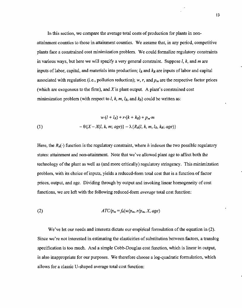
In this section, we compare the average total costs of production for plants in non-
attainment counties to those in attainment counties. We assume that, in any period, competitive
plants face a constrained cost minimization problem. We could formalize regulatory constraints
in various ways, but here we will specify a very general constraint. Suppose 1, k, and m are
inputs of labor, capital, and materials into production; 1R and kR are inputs of labor and capital
associated with regulation (i.e., pollution reduction); w, r, and Pm are the respective factor prices
(which are exogenous to the firm), andXis plant output. A plant's constrained cost
minimization problem (with respect to 1, k, m, 1R, and kR) could be written as:
w.(l + 1R) + r.(k + kR) +pmm
(1) — 0{X—X(l, k, m; age)} — A.{Rh(l, k, m, 1R, kR; age)}
Here, the Rh(.) function is the regulatory constraint, where h indexes the two possible regulatory
states: attainment and non-attainment. Note that we've allowed plant age to affect both the
technology of the plant as well as (and more critically) regulatory stringency. This minimization
problem, with its choice of inputs, yields a reduced-form total cost that is a function of factor
prices, output, and age. Dividing through by output and invoking linear homogeneity of cost
functions, we are left with the following reduced-form average total cost function:
(2) ATC/pm fh( w/pm, r/pm, X, age)
We've let our needs and interests dictate our empirical formulation of the equation in (2).
Since we're not interested in estimating the elasticities of substitution between factors, a translog
specification is too much. And a simple Cobb-Douglas cost function, which is linear in output,
is also inappropriate for our purposes. We therefore choose a log-quadratic formulation, which
allows for a classic U-shaped average total cost function:
14
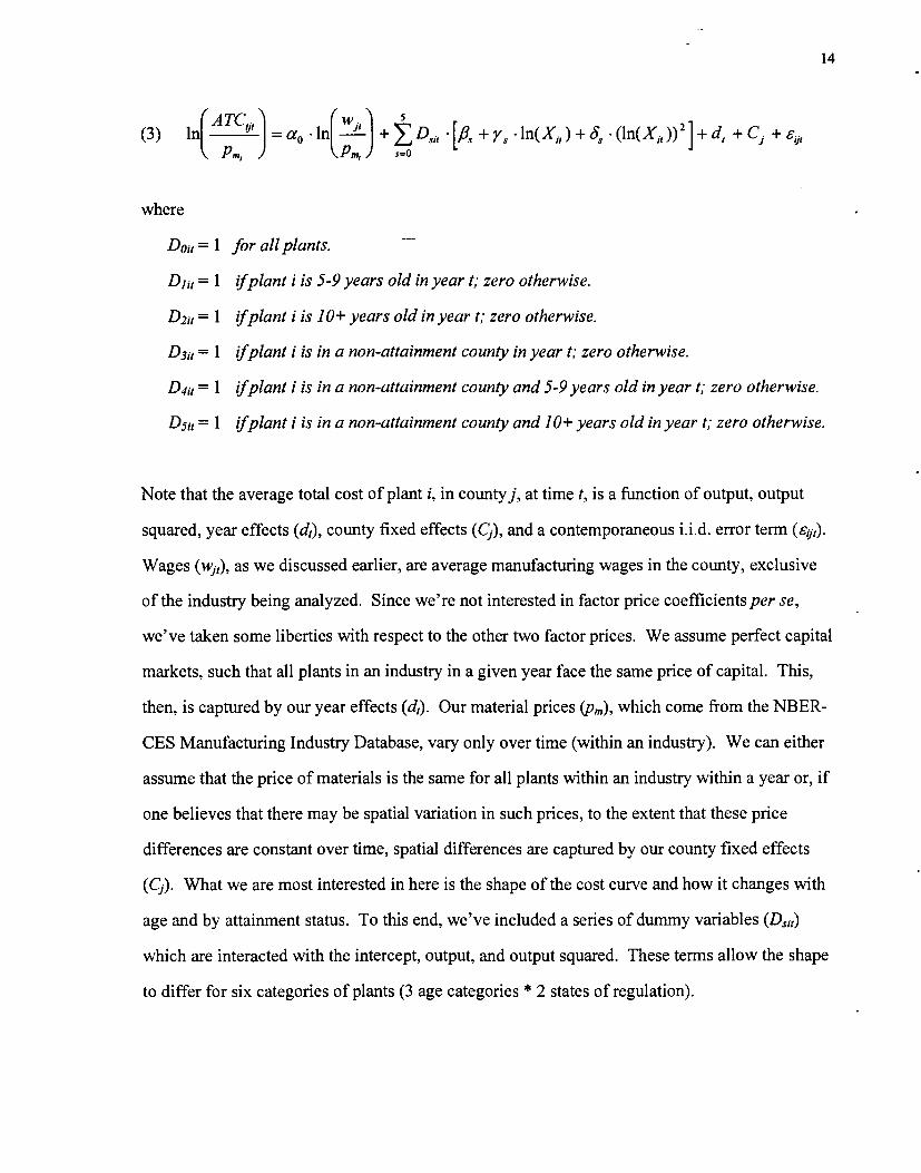
(3) in(ATJ =a0 .in[LJ +D51, •[i3 +y .1n(X,,)+o .(ln(X11))2]+d, +C +e,
where
D01, = 1 for all plants.
D111 = 1 fplant i is 5-9 years old in year t; zero otherwise.
D21 = 1 fplant i is 10+ years old in year t; zero otherwise.
D31 = 1 fplant i is in a non-attainment county in year t; zero otherwise.
D41 = 1 fplant i is in a non-attainment county and 5-9 years old in year t; zero otherwise.
D511 = 1 fplant i is in a non-attainment county and 10+ years old in year t; zero otherwise.
Note that the average total cost of plant i, in countyj, at time t, is a function of output, output
squared, year effects (d1), county fixed effects (Ci), and a contemporaneous i.i.d. error term (e1).
Wages (w), as we discussed earlier, are average manufacturing wages in the county, exclusive
of the industry being analyzed. Since we're not interested in factor price coefficients per se,
we've taken some liberties with respect to the other two factor prices. We assume perfect capital
markets, such that all plants in an industry in a given year face the same price of capital. This,
then, is captured by our year effects (di). Our material prices (pm), which come from the NBER-
CES Manufacturing Industry Database, vary only over time (within an industry). We can either
assume that the price of materials is the same for all plants within an industry within a year or, if
one believes that there may be spatial variation in such prices, to the extent that these price
differences are constant over time, spatial differences are captured by our county fixed effects
(C). What we are most interested in here is the shape of the cost curve and how it changes with
age and by attainment status. To this end, we've included a series of dummy variables (D,)
which are interacted with the intercept, output, and output squared. These terms allow the shape
to differ for six categories of plants (3 age categories *2 states of regulation).
15
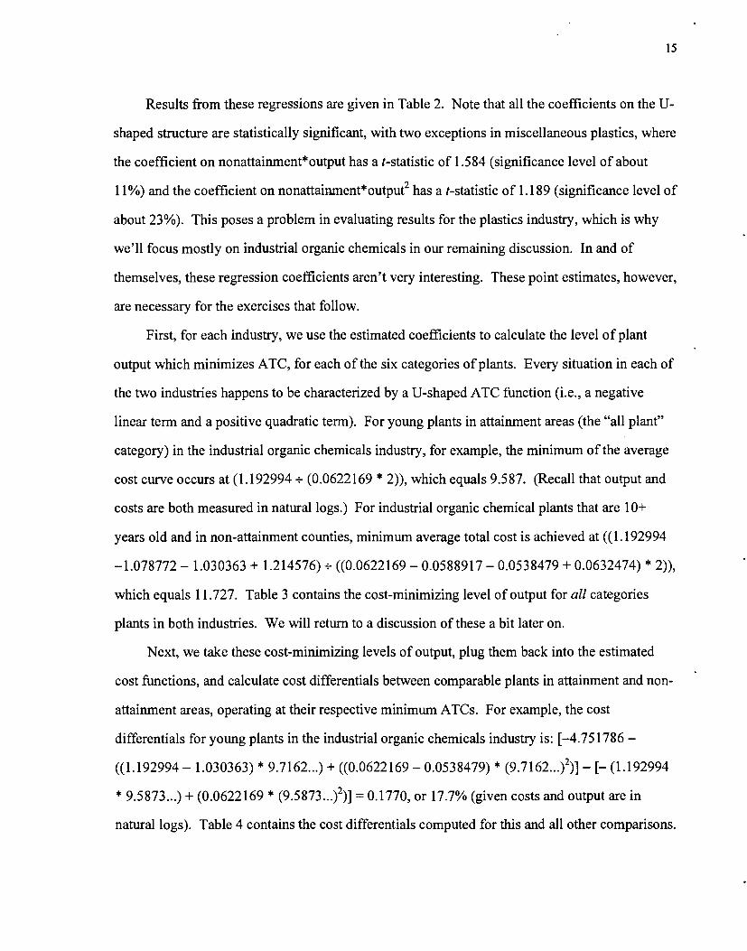
Results from these regressions are given in Table 2. Note that all the coefficients on the U-
shaped structure are statistically significant, with two exceptions in miscellaneous plastics, where
the coefficient on nonattainment*output has a t-statistic of 1.584 (significance level of about
11%) and the coefficient on nonattainment*output2 has a t-statistic of 1.189 (significance level of
about 23%). This poses a problem in evaluating results for the plastics industry, which is why
we'll focus mostly on industrial organic chemicals in our remaining discussion. In and of
themselves, these regression coefficients aren't very interesting. These point estimates, however,
are necessary for the exercises that follow.
First, for each industry, we use the estimated coefficients to calculate the level of plant
output which minimizes ATC, for each of the six categories of plants. Every situation in each of
the two industries happens to be characterized by a U-shaped ATC function (i.e., a negative
linear term and a positive quadratic term). For young plants in attainment areas (the "all plant"
category) in the industrial organic chemicals industry, for example, the minimum of the average
cost curve occurs at (1.192994 ÷ (0.0622169 * 2)), which equals 9.587. (Recall that output and
costs are both measured in natural logs.) For industrial organic chemical plants that are 10+
years old and in non-attainment counties, minimum average total cost is achieved at ((1.192994
—1.078772 — 1.030363 + 1.214576) ((0.0622 169 — 0.0588917 — 0.0538479 + 0.0632474) * 2)),
which equals 11.727. Table 3 contains the cost-minimizing level of output for all categories
plants in both industries. We will return to a discussion of these a bit later on.
Next, we take these cost-minimizing levels of output, plug them back into the estimated
cost functions, and calculate cost differentials between comparable plants in attainment and non-
attainment areas, operating at their respective minimum ATCs. For example, the cost
differentials for young plants in the industrial organic chemicals industry is: [—4.751786 —
((1.192994— 1.030363) * 9.7162...) + ((0.0622169 — 0.0538479) * (9.7l62...)2)] — [—(1.192994
* 9.5873...) + (0.0622169 * (9.5873...)2)] = 0.1770, or 17.7% (given costs and output are in
natural logs). Table 4 contains the cost differentials computed for this and all other comparisons.
16
Here (and throughout) differentials will be defined as the percent by which costs in non-
attainment areas exceed those in attainment areas. These are, therefore, expected to be positive.
The results in Table 4 indicate that costs are indeed higher for plants in non-attainment
areas, compared to those of similar age in attainment areas. In industrial organic chemicals,
young plants in non-attainment areas experience .costs 17.7% higher than their counterparts in
attainment areas. The difference for older plants, though lower, is still quite considerable, at
roughly 10%. This lower cost differential for older plants is consistent with the notion
(discussed earlier) that regulatory requirements are stricter for new (rather than existing) plants.
In the miscellaneous plastic products industry, production costs are also found to be more
expensive for plants in non-attainment counties, but the pattern is the reverse. Young plants in
non-attainment areas are found to have costs that are 4.3% higher than their counterparts in
attainment areas, while plants 5-9 years of age in non-attainment areas have 8.6% higher costs
and plants 10+ years of age have 11.2% higher costs. But again, the precision and accuracy of
these estimates are compromised by the two statistically insignificant cost function coefficients
used in their calculation. Nonetheless, all these results point in the same direction: non-
attainment status leads to higher operating costs for plants in these industries.
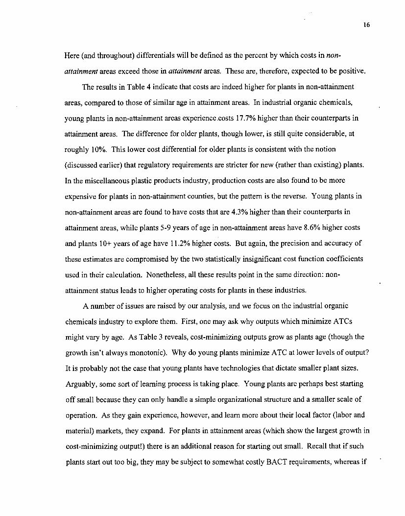
A number of issues are raised by our analysis, and we focus on the industrial organic
chemicals industry to explore them. First, one may ask why outputs which minimize ATCs
might vary by age. As Table 3 reveals, cost-minimizing outputs grow as plants age (though the
growth isn't always monotonic). Why do young plants minimize ATC at lower levels of output?
It is probably not the case that young plants have technologies that dictate smaller plant sizes.
Arguably, some sort of learning process is taking place. Young plants are perhaps best starting
off small because they can only handle a simple organizational structure and a smaller scale of
operation. As they gain experience, however, and learn more about their local factor (labor and
material) markets, they expand. For plants in attainment areas (which show the largest growth in
cost-minimizing output!) there is an additional reason for starting out small. Recall that if such
plants start out too big, they may be subject to somewhat costly BACT requirements, whereas if
17
they start out small they face no regulation. These small (initially) unregulated plants may then
expand as they learn more about their local regulatory environment, and in particular, as they
learn from other plants in the area how to best handle (or avoid) regulation. For plants in non-
attainment areas, which exhibit smaller changes in cost-minimizing output, there are reasons
(discussed previously) for not phasing-in investments this way.
Another issue, revealed in Table 5, is that the output of the "average" plant can be far
smaller than the level of output which minimizes ATC. There are a few reasons why this might
be. It may be the case that regional goods markets are imperfectly competitive, leading firms to
exercise some monopoly power (hence, production shy of cost-minimizing output). Risk
avoidance behavior (to reduce exposure) may also lead firms to invest less than what is
necessary to minimize average total cost. Having said that, however, we note that the differences
between actual and cost-minimizing output in attainment areas is absolutely enormous. For
plants 5-9 years of age in the industrial organic chemicals industry, the level of output that
minimizes ATC (12.46) is about 1.76 standard deviations from the average ln(output) of 9.96,
and the gap for plants 10+ years of age is even larger! What is limiting the size of these plants?
The obvious suggestion is regulation, or more specifically, the threat of regulation. If one
believes these particular extrapolations out to the cost-minimizing levels of output, there are
(virtually) decreasing average total costs throughout. Plants in attainment areas do not generally
grow to these sizes because at some point they will attract attention from regulators; they will be
sued by local interest groups; they may even (single-handedly) pollute their counties into non-
attainment. There are, therefore, regulation-related constraints even on these "unregulated"
plants (that don't get reflected in production costs). The plants that do grow to these sizes may
be in lax states, where plants in attainment areas really are left alone —that is, areas that truly
are devoid of effective regulation.
The oldest category of plants in attainment areas also contain two distinct groups: those
built before the regulatory era (say, the 1970 amendments to the Clean Air Act) and those built
after. Recall that we acknowledged this distinction (i.e., pre- and post-1968 plants) in our
18
investment regressions above. Attempts to control for this separate group of plants here in our
cost functions resulted in coefficients insignificant at the 5% level. However, the coefficients
(albeit imprecise as they are) suggested that plants built before 1968 have much larger cost-
minimizing levels of output than other plants 10+ years of age. The estimates suggested that
those pre-1968 plants could operate at much lower costs in attainment areas if they operated at a
large scale — large enough to be regulated, but much less severely than they would be in a non-
attainment area. Post-1968 plants that are 10+ years of age, on the other hand, operated at about
the same costs in attainment and non-attainment areas. (Differentials for young plants and those
5-9 years of age are unaffected by this re-formulation.) All this might suggest that large pre-
1968 plants in attainment areas, as grandfathered players with extensive experience, reap
considerable advantages. Having said that, however, it is still the case that very few of these
plants operate at even a reasonable fraction of cost-minimizing output. We are, therefore, left
with our same conclusion: plants in attainment areas stay small to avoid triggering regulation.
How do differences between the estimated cost-minimizing levels of output and the actual
levels of plant output affect the cost differentials computed in Table 4? To see, we repeated the
above exercise using instead average ln(output) and ln(average output). The results of these (and
our previous) computations for the industrial organic chemicals industry are contained in Table
6. The cost differentials for young plants is fairly insensitive to the output measure chosen.
Using average ln(output), young plants are found to have costs 16.7% higher in non-attainment
areas, compared to their counterparts in attainment areas. Using /n(average output), this
difference was found to be 16.0%. Originally, using ATC-minimizing output, we had found a
cost differential of 17.7%. For the older categories of plants, the results are less comparable
across output measures. Using average ln(output), cost differentials all but disappear for plants
over 5 years of age (+1.3% and —1.8%). With ln(average output), plants 5-9 years of age are
found to have costs 9.0% higher in non-attainment areas (versus 9.9%, using cost-minimizing
output), but differences virtually disappear (+0.2%) for plants 10+ years of age. All of these
estimates, however, recalling our earlier discussions, are likely to represent lower bounds on the
19
true costs of regulation. If nothing else, they uniformly indicate that regulation is most
burdensome for new (rather than existing) plants.
An Alternative Approach
Instead of quantifying the costs of regulation by inferring it indirectly from a plant's total
costs (which we did in the previous section), one could also, in principle, examine directly the
environmental costs incurred by the plant. The Census Bureau's Pollution Abatement Costs and
Expenditure (PACE) survey, for example, asks manufacturing plants about their capital
expenditures and operating costs associated with various environmental efforts. This survey,
however, has been criticized for potentially missing a large portion of environmental expenses
(see Jaffe, et a!. (1995) for a discussion). It is generally the case that plants do not keep special
track of their expenditures on environmental protection. These data therefore must be estimated.
Capital expenditures of the "end-of-line" variety (e.g., scrubbers, filters, precipitators, and so
forth) are rather straightforward to estimate, since these items are easily identifiable and their
sole purpose is pollution abatement. However, when capital expenditures are of the "production
process enhancement" type (e.g., the installation of new equipment which improves production
efficiency and reduces air emissions) the task is much more difficult.
In these instances, survey respondents are asked to "estimate the pollution abatement
portion [of such projects] as the extra cost of pollution abatement features in structures and
equipment (i.e., your actual spending less what you would have spent without the pollution
abatement features built-in)." The Census Bureau (1994) acknowledges that "interviews with
survey respondents indicate that estimating such an incremental cost is difficult in many
instances" ... ifnot impossible. In 1992, the following "special instructions" were added to the
survey form to help respondents in particularly difficult cases:
"Do not include any of the project cost unless the primary purpose is
environmental protection. If the primary purpose of the project is
environmental protection, report the whole production process enhancement
20
project expenditure.... Caution: A project with the primary purpose of
improving production efficiency may include pollution abatement features
added to meet legal requirements. Since the primary purpose of such a project
is still not environmental prutection, do not report any of the production
process enhancement."
Given these guidelines, and the last two sentences in particular, it is not clear whether any of the
costs of production equipment meeting strict LAER standards, for example, will be attributed to
environmental protection and reported in PACE, especially in the absence of an obvious
baseline.
Concerns also apply to operating expenses. The salaries and wages of a plant's
environmental staff are rather easily accounted for, but what of a production team who spends a
small but non-zero amount of time on various "environmental tasks" or of plant management
who must also spend a fraction of its time and effort on environmental issues? Do these costs get
captured in PACE? Similarly, the cost of "materials, parts, and components that were used as
operating supplies for pollution abatement, or used in repair or maintenance of pollution
abatement capital assets" might be easy to estimate, but what about the "incremental costs for
consumption of environmentally preferable materials and fuels" or the "fuel and power costs for
operating pollution abatement equipment"? Surely these are not easy items to calculate, even for
the most talented and organized (and patient) of plant staffs. Apart from the potential under-
reporting of capital expenditure and operating costs, there are certainly other potential costs that
PACE makes no attempt to capture. For example, adverse impacts on plant output, either from
the outright stoppage of production (e.g., to install pollution control devices) or through the loss
of operational flexibility (to comply with certain regulatory requirements). All these factors
argue for the approach we used in the previous section, where environmental costs (and related
effects) are subsumed by total plant costs (and output).
Nevertheless, we conducted some rudimentary analysis of our two industries using plant-
level data from the 1992 PACE survey linked to 1992 Census of Manufactures (CM) data from
21
the LRD. Only a relatively small sample of manufacturing plants are actually asked to complete
the PACE survey in any given year (e.g., approximately 17,000 in 1992), focusing
disproportionately on large (and hence older) plants and plants in polluting industries. After
eliminating plants with imputed dat&(in either the PACE, the CM, or both), as well as other
suspicious cases, we are left with approximately 15% of all plants in industrial organic chemicals
in 1992 and about 4.5% of all plants in miscellaneous plastic products. This is about one-third
the industry coverage we had in our above cost function exercises. And young plants, a segment
we found to be particularly affected by regulation in our above work, are under-represented here
in our PACE-LRD samples. In industrial organic chemicals, only 7% of our sample consists of
young plants (compared to 23% of the 1992 population in this industry), and in miscellaneous
plastics, 13% are young plants (compared to 35% in the 1992 population). In our above work,
using just multi-unit plants from 1972-1992, young plants accounted for 15% and 26% of our
samples, respectively, compared to the 16% and 30% in the universes from which they were
drawn. These differences in sample sizes and composition, as well as in the time period covered,
should be kept in mind when comparing the results here to the ones found above. In particular,
an unfortunate consequence of the limited number of young plants we have here is that we are
not able to properly distinguish separate age effects in what we do below.
Table 7 contains some basic statistics for our sample of plants. In particular, we present the
share of total plant capital expenditures, labor costs, and operating costs (in 1992) directly
attributable to air pollution abatement activity. These shares are gotten from comparing PACE
and CM responses to questions on capital investments; salaries and wages; and the costs of labor,
materials, energy (electricity + fuels), and contract work; respectively. Note that operating costs
as defined here (as opposed to what we used above) do not include the costs of "capital services"
(essentially because we do not have data on the stock of pollution abatement capital equipment).
What is perhaps most striking here is that expenditures on air pollution abatement in these
industries appears to be fairly low. Air pollution capital expenditures in industrial organic
chemicals only accounts for about 6.8% of total capital expenditure in our sample of plants
22
(6.9% based on published totals). In plastics, this number is under 2%. The share of plant labor
costs and operating costs accounted for by air pollution concerns in industrial organic chemicals
is 1.8% and 0.9% respectively. In miscellaneous plastics, these shares are negligible.
While the impact of regulationgenerally appears to be much smaller here than what we
were finding before, a direct comparison is not possible given the aforementioned difference in
the way operating costs are measured. We therefore instead turn to a comparison of costs
between plants in attainment and non-attainment areas, using the three cost measures that we do
have here. In particular, we run simple OLS regressions where our dependent variable is a
plant's ratio of air pollution abatement expenditures (capital investment, labor costs, or operating
costs) to total plant expenditures (in those same respective categories). Our explanatory
variables include plant output, plant age, a "multi-unit" dummy, and county ozone non-
attainment status. The non-attainment coefficients from these regressions are reported in Table
8. Only relative capital expenditure on air pollution abatement in industrial organic chemicals is
significantly higher in non-attainment areas than it is in attainment areas, with a difference of
almost 4%. All the other non-attainment coefficients are statistically insignificant and very close
to zero.
These estimates obviously suggest much lower regulatory costs than what we were finding
with our cost function approach in the previous section. This might be evidence of the long-held
belief that PACE misses a substantial portion of environmental expenditures. The potential
limitations of this survey (noted above) would obviously understate costs much more for plants
in non-attainment areas than those in attainment areas, narrowing the estimated gap between the
two groups. Our earlier caveats, regarding possible self-selection as well as "voluntary"
environmental expenditures, also apply here —serving to narrow this gap even more. And we
note again that our results in Table 8 do not (because we really cannot) distinguish regulatory
effects by age. Given our previous results, indicating that young plants are most affected by
regulation, and given that the PACE sample is actually weighted toward older plants, differences
in cost estimates may also (to some extent) be due to differences in sample composition. That
23
this potentially heavily-affected group is under-represented in PACE obviously also has potential
implications for the aggregate statistics published from this survey. The results here are
suggestive, but much more work is needed in this area.
Conclusions
This paper examines the effects air quality regulation has had on the size and timing of
plant investment in two particular industries, and the cost such regulation poses on firms in these
industries. In the industry with high relative average capital assets, we find that new, regulated
plants start out much larger than their unregulated counterparts but then do not invest as much,
such that after 10 years, capital stocks of regulated plants are in fact smaller. This is consistent
with our previous findings and highlights the substantial fixed costs involved in negotiating
expansion permits, the benefits of preserving one's "grandfathered" status, and the desire to stay
small (or even downsize) in an environment where the amount of regulatory attention is often
correlated with plant size. In terms of quantifying the costs of air quality regulation, our basic
results show that heavily-regulated plants indeed face higher production costs than their less-
regulated counterparts. This is particularly true for younger plants, which is consistent with the
notion that regulation is most burdensome for new (rather than existing) plants. "Unregulated"
plants, however, also appear to affected by regulation (or at least the threat of regulation), as we
found that they produce at levels far short of the levels that minimize average total costs. This,
again, demonstrates the role plant size plays in regulatory efforts.
24
Notes
1. In theory, one might control for self-selection by using plant fixed effects in modeling
(rather than county fixed effects, which we use here). In practice, however, imposing plant fixed
effects eliminates many young plant&(since these fixed effects require each plant to appear in
two Censuses, at least five years apart), makes identification of age effects impossible, and
greatly reduces sample sizes. We therefore resign ourselves to any selection bias that may be
present, realizing that it will reduce our estimates of treatment effects.
2. Note that, even with regulation, non-attainment counties do have some births, given a local
supply of entrepreneurs (with their own idiosyncrasies) and local and regional demand forces.
3. Total assets (buildings and machinery together) was also asked of non-ASM plants in the
1987 and 1992 Censuses. For our cost function exercises, since we are not interested in the
separate components of capital stock, we also use these plants in our estimation.
4. In industrial organic chemicals, corporate plants account for about 97% of the industry's
output. In miscellaneous plastic products, they account for about 72%.
5. For example, a plant in the 1972 Census is 0-4 years of age if it is making its first Census
appearance in 1972. It is 5-9 years of age if it made its first Census appearance in 1967 and 10+
years of age if it made its first Census appearance in the 1963 Census. The recognition of any
additional age categories is not practical. Since the LRDdoes not contain any of the Censuses
prior to 1963, one is not able to distinguish between 1972 plants that are 10-14 and 15+ years of
age. Excluding 1972 plants from the analyses (and using just 1977-1992 plants) avoids this
problem but unfortunately eliminates an important (control) group of pre-regulatoiy plants which
help us identify the effects of regulation. On the opposite end,fewer age categories would not
buy us any additional data. In principle, two age categories would allow us to use plants in the
1967 Census as well, however capital asset data were not collected from these plants and
therefore they are of no use to us for the types of analyses we wish to conduct here. Three age
categories, therefore, is most ideal.
25
6. The difficulty here is that that the asset information collected by the Census Bureau is on
an 'original cost' basis. It reflects the book value of assets (of various vintages and quality and
so forth) but not necessarily their true economic value. Given the highly imperfect nature of
these data, multiplying them by apraper user cost of capital series seems somewhat
incongruous. What we've done instead is. derive "user cost factors" such that capital's share of
total costs in our samples (by industry and year) equal capital's share of total output (for the
corresponding year and 2-digit industry) in Dale Jorgenson's 35KLEM.DAT (available at his
Harvard University website and described in Jorgenson (1990)). For SIC 28 (Chemicals),
capital's share of total output in Jorgenson's data ranged from 15.2% (1982) to 21.3% (1987), for
the five Census years used in our study. To replicate these shares in our data for industrial
organic chemicals required user cost factors ranging from .1495 (1972) to .2136 (1987). For SIC
30 (Rubber and Miscellaneous Plastics), capital's share of total output in Jorgenson's data ranged
from 4.1% (1982) to 6.6% (1972). To replicate these shares in our miscellaneous plastic
products sample required user cost factors ranging from .0689 (1982) to .0979 (1972). We note
that in the initial phases of this study we experimented with time-invariant user cost factors of
.17 (e.g., a 10% interest rate plus a 7% depreciation rate) and .10, with results that are
remarkably similar to the ones obtained using the factors computed above. We do not believe,
therefore, that our results are sensitive to our treatment of the capital data.
7. [(1 + 0.968 + 0.794 - 1.046) -(1 + 0.968)] ÷ (1 + 0.968)= -0.1280, or roughly 13%.
8. [(1 + 0.968 + 0.793 + 0.794 - 1.046 + 0.555) - (1 + 0.968 + 0.793)] ÷ (1 + 0.968 + 0.793) =
0.1097, or 11%.
9. Having said that, an identical regression (not reported here) on a sample that also includes
single-unit firms (in addition to these multi-unit plants) reveals some of the hypothesized effects.
Namely, new plants in non-attainment areas were found to start with 20% more capital than their
counterparts in attainment areas, but after 10 years, there was virtually no difference between the
two groups. Why these effects might be found in the single-plant sector and not the multi-plant
"corporate" sector is puzzling.
26
References
Barteisman, Eric J., Randy A. Becker, and Wayne B. Gray. NBER-CES Manufacturing Industry
Database. (Available via the Internet at the NBER website.)
Bartik, Timothy J. 1988. "The Effect&of Environmental Regulation on Business Location in the
United States," Growth and Change, 19(3), 22-44.
Becker, Randy A. 1998. The Effects of Environmental Regulation on Firm Behavior. Brown
University Ph.D. Thesis.
Becker, Randy A. and J. Vernon Henderson. 2000. "Effects of Air Quality Regulation on
Polluting Industries," Journal of Political Economy, forthcoming.
—. 1997. "Effects of Air Quality Regulation on Decisions of Firms in Polluting Industries,"
NBER Working Paper Series, 6160.
Gray, Wayne B. 1996. "Does State Environmental Regulation Affect Plant Location?" Clark
University mimeo.
Henderson, J. Vernon. 1996. "Effects of Air Quality Regulation," American Economic Review,
86(4), 789-8 13.
Jaffe, Adam B., Steven R. Peterson, Paul R. Portney, and Robert N. Stavins. 1995.
"Environmental Regulation and the Competitiveness of U.S. Manufacturing: What Does
the Evidence Tell Us?" Journal of Economic Literature, 33(1), 132-163.
Jorgenson, Dale W. 1990. "Productivity and Economic Growth," in F/iy Years of Economic
Measurement, Ernst R. Berndt and Jack E. Triplett (eds.). NBER Studies in Income and
Wealth, vol. 54. Chicago: University of Chicago Press.
Levinson, Arik. 1996. "Environmental Regulation and Manufacturers' Location Choices:
Evidence from the Census of Manufactures," Journal of Public Economics, 62(1), 5-29.
McConnell, Virginia D. and Robert M. Schwab. 1990. "The Impact of Environmental Regulation
on Industry Location Decisions: The Motor Vehicle Industry," Land Economics, 66(1), 67-
81.
U.S. Bureau of the Census. 1994. Pollution Abatement Costs and Expenditures, 1992.
Washington, DC: U.S. Government Printing Office.
27

</ref_section>
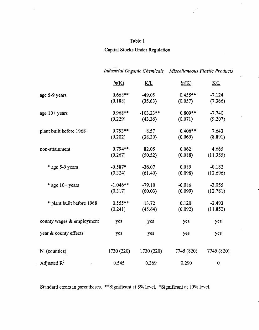
Table 1
Capital Stocks Under Regulation
Industrial Organic Chemicals Miscellaneous Plastic Products
ln(K KJL ln(K) ILL
age 5-9 years 0.668** -49.05 Ø455** 7.124
(0.188) (35.63) (0.057) (7.366)
age l0+years 0.968** 103.23** 0.809** -7.740(0.229) (43.36) (0.071) (9.207)
plant built before 1968 0.793** 8.57 0.406** 7.643
(0.202) (38.30) (0.069) (8.891)
non-attainment Ø•794** 82.05 0.062 4.665
(0.267) (50.52) (0.088) (11.355)
*age 5-9 years 0.587* -36.07 0.089 -0.182
(0.324) (61.40) (0.098) (12.696)
*agelo+years 1.046** -79.10 -0.086 -3.055(0.317) (60.03) (0.099) (12.781)
*plantbujltbefore 1968 0.555** 13.72 0.120 -2.493
(0.241) (45.64) (0.092) (11.852)
county wages & employment yes yes yes yes
year & county effects yes yes yes yes
N (counties) 1730 (220) 1730 (220) 7745 (820) 7745 (820)
Adjusted R2 - 0.545 0.369 0.290 0
Standard errors in parentheses. **sigthficant at 5% level. *sigthflcant at 10% level.
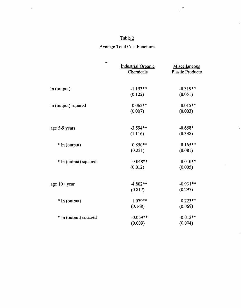
Table 2
Average Total Cost Functions
Industrial Organic MiscellaneousChemicals Plastic Products
in (output) 1.193** 0.3l9**(0.122) (0.051)
in (output) squared 0.062** 0.015**
(0.007) (0.003)
age 5-9 years ..3594** O.658*(1.116) (0.338)
*ln(output) 0.850** 0.165**
(0.231) (0.081)
* in (output) squared 0.048** -0.0i0(0.012) (0.005)
age 10+year 4.802** 0.931**(0.817) (0.297)
*ln(output) 1.079** 0.223**
(0.168) (0.069)
* in (output) squared 0.059** 0.012**
(0.009) (0.004)
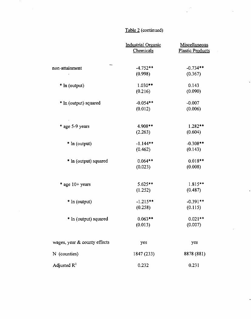
Table 2 (continued)
Industrial Organic MiscellaneousChemicals Plastic Products
non-attainment 4.752** 0.734**(0.998) (0.367)
*ln(output) 1.030** 0.143
(0.216) (0.090)
* In (output) squared 0.054** -0.007(0.012) (0.006)
*age5..9 years 4.908** 1.282**
(2.263) (0.604)
* in (output) 1.144** 0.308**(0.462) (0.143)
*ln(output) squared 0.064** 0.018**
(0.023) (0.008)
*agelo+years 5.625** 1.815**
(1.252) (0.487)
* in (output) _1.215** _0.391**
(0.258) (0.115)
*ln(output) squared 0.063** 0.021**
(0.013) (0.007)
wages, year & county effects yes yes
N (counties) 1847 (233) 8878 (881)
AdjustedR2 0.232 0.231
Standard errors in parentheses. **sigthficant at 5% level. *sigthficant at 10% level.
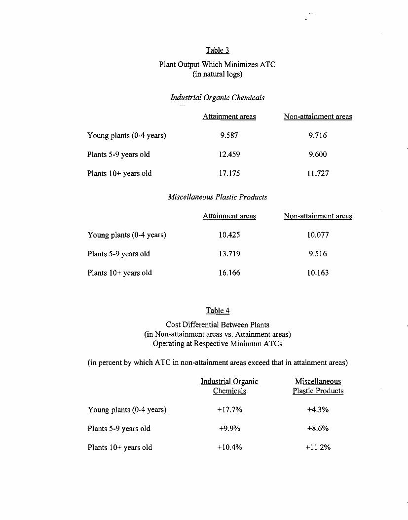
Table 3
Plant Output Which Minimizes ATC(in natural logs)
Industrial Organic Chemicals
Attainment areas Non-attainment areas
Young plants (0-4 years) 9.587 9.7 16
Plants 5-9 years old 12.459 9.600
Plants 10+ years old 17.175 11.727
Miscellaneous Plastic Products
Attainment areas Non-attainment areas
Young plants (0-4 years) 10.425 10.077
Plants5-9yearsold 13.719 9.516
Plants 10+yearsold 16.166 10.163
Table 4
Cost Differential Between Plants(in Non-attainment areas vs. Attainment areas)
Operating at Respective Minimum ATCs
(in percent by which ATC in non-attainment areas exceed that in attainment areas)
Industrial Organic MiscellaneousChemicals Plastic Products
Young plants (0-4 years) +17.7% +4.3%
Plants 5-9 years old +9.9% +8.6%
Plants 10+ years old +10.4% +11.2%
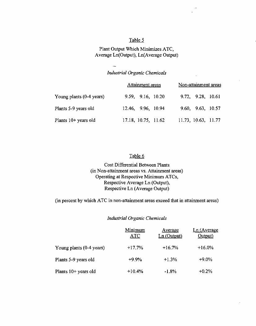
Table 5
Plant Output Which Minimizes ATC,
Average Ln(Output), Ln(Average Output)
Industrial Organic Chemicals
Attainment areas Non-attainment areas
Young plants (0-4 years) 9.59, 9.16, 10.20 9.72, 9.28, 10.61
Plants 5-9 years old 12.46, 9.96, 10.94 9.60, 9.63, 10.57
Plants 10+yearsold 17.18, 10.75, 11.62 11.73, 10.63, 11.77
Table 6
Cost Differential Between Plants(in Non-attainment areas vs. Attainment areas)
Operating at Respective Minimum ATCs,Respective Average Ln (Output),Respective Ln (Average Output)
(in percent by which ATC in non-attainment areas exceed that in attainment areas)
Industrial Organic Chemicals
Minimum Average Ln (AverageATC Ln (Output) Output)
Young plants (0-4 years) +17.7% +16.7% +16.0%
Plants 5-9 years old +9.9% +1.3% +9.0%
Plants 10+ years old +10.4% -1.8% +0.2%
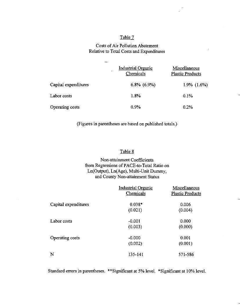
Table 7
Costs of Air Pollution AbatementRelative to Total Costs and Expenditures
Industrial Organic MiscellaneousChemicals Plastic Products
Capital expenditures 6.8% (6.9%) 1.9% (1.6%)
Labor costs 1.8% 0.1%
Operating costs 0.9% 0.2%
(Figures in parentheses are based on published totals.)
Table 8
Non-attainment Coefficientsfrom Regressions of PACE-to-Total Ratio onLn(Output), Ln(Age), Multi-Unit Dummy,
and County Non-attainment Status
Industrial Organic MiscellaneousChemicals Plastic Products
Capital expenditures 0.038* 0.006(0.021) (0.004)
Labor costs -0.00 1 0.000(0.003) (0.000)
Operating costs -0.000 0.00 1
(0.002) (0.001)
N 135-141 571-586
Standard errors in parentheses. **Significant at 5% level. *Significant at 10% level.