Embed Size (px)
Citation preview

Counter-current gas-liquid contacting in a
Rotating Spiral Channel: Experimental
and Theoretical Study
A Thesis
submitted to the University of Sheffield for the degree of Doctor of
Philosophy in the Faculty of Engineering
By
Ahmed A. A. AYASH
Chemical and Biological Engineering Department,
The University of Sheffield,
United Kingdom.
July 2018

I
Dedication
To my late parents who taught me to love learning, my
wonderful wife Milad for her support and my lovely daughters
Dema & Dana who wonder what I do all the day.
Ahmed AYASH

II
Acknowledgments I would like to express my deepest gratitude to all my family, friends and colleagues
who have contributed in finishing this work. I spent almost four years working on this
thesis and during this time many people have helped in one way or another to make this
work happen.
First of all, I would like to thank my supervisor ‘Dr Jordan MacInnes’ for his many
hours of guidance, patience and material support for this work. Jordan was always
available, no matter how busy, to discuss and comment critically on the theoretical and
practical aspects of the work. His knowledge, wisdom and enthusiasm in the work are
unrivalled, I feel lucky to be supervised by him. I also must thank Professor Willam
Zimmerman and Dr Willam Furnass for their help to provide access to Sheffield’s high-
performance computing system (iceberg). I want to thank also Dr George Dowson for
the helpful discussion regarding the safe handling of the chemical materials used in the
experiments.
Thanks and appreciation go to all the technicians in our department. Particularly, Mr
Mark McIntosh, Mr Mark Jones, Mr James Grinham, Mr Keith Penny and Mr Usman
Younis for their appreciable efforts in fixing technical problems experienced during this
work. I want to thank also Mr Robert Hanson in the chemistry department/University of
Sheffield for helping in the analysis process of the samples.
Special thanks to my wife ‘Milad’ for her understanding, patience and sacrifice for
bearing my period of study. Without her support, this work would not have been finished.
I owe her. I would like to thank my sister ’Areej’ and my wife’s father ‘Mr Adel
Mahmoud’ for their continuous support in Iraq throughout my doctoral journey. I also
must thank my friend ‘Dr Khalid Murshid’ for his support and all the staff of
Materials Engineering Department in Al-Mustansriya University. Many thanks to my
lovely daughters ‘Dema & Dana’ who have shown outstanding patience
as I have not been able to spend much time with them.
Last, but not least, I thank my country represented by ‘the Higher Committee for
Education Development in Iraq’ for scholarship and every individual in my country as
each of them contributes in the fund of this scholarship.

III
Abstract
Controlled counter-current contacting between a gas and a liquid forms the basis for
a wide range of chemical separation operations, including absorption, stripping and
distillation. A radical technique based on the rotating of a spiral channel can achieve
segregation of any two immiscible phases into two parallel layers, allowing for a detailed
control of phase flow rates and phase layer thicknesses. This work experimentally and
theoretically studied the mass transfer process of gas-liquid contacting in this novel
contactor, aiming for understanding, evaluating and demonstrating its performance.
In order to establish the spiral performance, experiments were conducted over a wide
range of contacting conditions. In the experiments, desorption of four different organic
solutes from water was studied separately at dilute concentrations, using air as a sweeping
gas. The solutes were ethanol, acetonitrile, acetone and 2-butanone (MEK). This
collection of solutes at different spiral temperatures (24, 30 and 49°C) gives a range of
solute equilibrium distributions ( ) from 0.232 to 5.5 (the mole fraction ratio of solute
in the two phases). Thus, the performance of the rotating spiral channel was explored
using phase and solute systems having different equilibrium characteristics ( ) and
solute transferring properties. The other contacting conditions were the pressure and the
rotation rate, which were fixed to 1.8 bara and 3200 rpm, respectively. For each phase
and solute system ( ), the amount of solute desorbed was measured over a range of
phase flow rates. Interestingly, the results showed that a fixed channel design can process
a variety of systems at any desired conditions, producing solute-free water when operating
at the appropriate phase flow rate ratio. Furthermore, the experimental results showed a
universal peak in the mass transfer coefficient at a liquid layer thickness between 80-90
µm. The peak occurred independently of the gas phase flow rate and appeared
prominently for the systems with large , where the mass transfer was much affected
by the liquid phase. This finding indicates that independent adjustment of the liquid phase
flow rate could determine the optimum contacting and this optimum can be tailored to
occur at any desired phase flow rates ratio by changing only the gas phase flow rate.
Thus, simultaneously, the optimal contactor size and solvent usage could be achieved
with rotation spiral contacting.
f
f
f
f

IV
In addition, the spiral performance, based on the extensive data of the current work,
was compared to the performance for the conventional packed column, rotating packed
beds and the membrane microchannel using data from the literature for these contactors.
The normalised total specific throughput (molar flow rate of the treated stream divided
by the contactor volume) was developed here and used as the comparison criterion. The
maximum of this measure corresponds to a minimum contactor volume to achieve a given
separation task. The comparison showed that the rotating spiral was able to operate in the
appropriate range of phase flow rate ratios and gave the highest specific throughput. This
suggests that the contactor size for this method can be many times smaller than that of the
other methods considered.
A two-dimensional (2-D) computational model was adopted in this work to study the
detail of the flow and species fields that determine the mass transfer process. This model
is based on a novel combination of the governing equations and an existing interface
model to capture accurately the Coriolis acceleration effects and phase interactions. The
2-D model effectively predicted a wide range of experimental conditions, demonstrating
that Coriolis secondary motion could double the mass transfer performance. A parametric
study was also conducted using the 2-D model, where desorption of acetone was taken as
a reference case. The purpose of this study was to examine the role of three key
parameters (rotation rate, channel aspect ratio and flow rate of both phases) that were not
tested experimentally. The results demonstrated that by adjusting the rotation rate ( ),
the contacting process could be optimised. For a range between 1000 and 20,000 rpm, it
was found that =16,000 rpm gave a maximum mass transfer coefficient. Furthermore,
the data showed that the spiral performance was enhanced considerably by changing the
channel aspect ratio. Reducing the channel width from 4 mm to 1 mm increased the mass
transfer coefficient by a factor of two. Finally, at a given rotation rate and channel aspect
ratio, an improvement in mass transfer was observed by adjusting the flow rates of the
contacting phases. Increasing the flow rate of both phases increased the mass transfer
coefficient also by a factor of two.
In general, the experimental and theoretical work in this thesis demonstrate the
potential of rotating spiral contacting and establish a useful foundation underpinning its
future development.

V
Main Publications
Ayash, A. A. and MacInnes, J. M., 2017. Mass Transfer Prediction of Gas-Liquid
Contacting in a Rotating Spiral Channel. in the 4th International Conference of
Fluid Flow, Heat and Mass Transfer (FFHMT’17). Toronto, Canada, pp. 1–8.
MacInnes, J.M. and Ayash, A.A., 2018. Mass transfer characteristics of rotating
spiral gas-liquid contacting. Chemical Engineering Science, 175, pp.320–334.
Ayash, A. A. and MacInnes, J. M., 2018. 2-D parametric analysis of Gas-Liquid
Contacting in a Rotating Spiral Channel. To be submitted.

VI
Nomenclature
Symbol Definition
A Area, m2
a Interfacial surface area per passage volume, m2/m3
12a and 21a Adjustable parameters of UNIQUAC model
La Purity of the heavy phase (solvent) in absorption process
Va Purity of the light phase (target phase) in absorption process
D Solute diffusion coefficient, m2/s
Ld Purity of the heavy phase (target phase) in desorption process
Vd Purity of the light phase (solvent) in desorption process
Eo Eötvös number (ratio of the centrifugal force to the interfacial force)
Ek Ekman number (ratio of viscous force to Coriolis force)
f Slope of solute equilibrium relation, )( LV YfY =
Fr Froude number (ratio of inertial force to centrifugal force)
g Gravity acceleration, 9.81 m/s2
h Channel height, m
Lmh Minimum liquid layer thickness, mm
mh Interface meniscus height, m
j Solute molar flux across the phase interface, Kmol/m2/s
K Overall mass transfer coefficient, Kmol/m2/s
k Individual mass transfer coefficient, Kmol/m2/s
L Contact length, m
Diffusion length, m
I Length of phase interface, m
e Length of one equilibrium stage, m
M Molar mass, kg/kmol
N Molar flow rate, Kmol/s
Ne Number of equilibrium stages
NE Number of elements used in the numerical computations

VII
n Molar density, Kmol/m3
p Pressure, Pa
p Piezometeric pressure, Pa
Pe Péclet number (ratio of mass transfer by fluid motion to
mass transfer by molecular diffusion)
Q Volumetric flow rate, m3/s
LCQ Liquid phase volumetric flow rate in the meniscus region, m3/s
q Phase volumetric flow rates ratio, LV QQq =
nq Phase molar flow rates ratio, LLVVn QnQnq =
nCq Critical molar flow rates ratio
R Spiral radius, m
Re Reynolds number (ratio of inertial force to viscous force)
Ro Rossby number (ratio of inertial force to Coriolis force)
r Interface radius, m
Sc Schmidt number (ratio of momentum diffusivity to mass diffusivity)
T Temperature, oC or K
t Spacing distance between spiral channels, m
mt Residence time, s
St Sampling time, s
u Velocity component in x direction, m/s
V
Velocity vector, m/s
v Velocity component in y direction, m/s
V Root-mean-square velocity,
+=
AA
dAvdAuA
V 221
W Spiral channel width (direction parallel to the phase interface), m
w Velocity component in z direction, m/s
We Weber number (ratio of inertial force to interfacial force)
Y Solute mole fraction
x, y, z Cartesian Coordinates

VIII
Greek Symbols
Symbol Definition
Spiral angle, degrees or radians
Conservative flux vector in Comsol Multiphysics Software
Liquid phase activity coefficient
r Ratio of the centrifugal force to the pressure force
C Capillary height, m
Void fraction
Azimuthal angle of spiral, degrees or radians
Ratio of the centrifugal force to the gravity force
Viscosity, Kg/m/s
Kinematic Viscosity, m2/s
Fraction of the passage volume occupied by the heavy phase
Density, kg/m3
σ Surface tension, N/m
Shear stress, Pa
Specific throughput, s-1
N Total Specific throughput, s-1
Rotation rate, rad/s (1 rad/s equivalent to 9.549 rpm)
Subscripts
Symbol Definition
B Bulk (mean value of velocity, concentration or pressure)
C Critical or corner
e Equilibrium
I Interface
L Heavy phase (liquid)
V Light phase (gas)
W Wall or Water
Superscripts

IX
Symbol Definition
* Normalised variable
∞ Infinite dilution
Sat Saturation
. Rate
Abbreviations
Symbol Definition
CFD Computational fluid dynamics
FEM Finite element method
MEK Methyl ethyl Ketone or 2-butanone
PDE Partial differential equation
rms Root mean square
UNIFAC UNIQUAC Functional-group Activity Coefficients model
UNIQUAC Universal QuasiChemical model
WCM Wide-channel model
X
Table of Contents
List of Figures XV
List of Tables XXIV
CHAPTER 1: INTRODUCTION ....................................................................................... 1
RESEARCH MOTIVATIONS AND OBJECTIVES ............................................................ 3
THESIS STRUCTURE .................................................................................................. 5
CHAPTER 2: BACKGROUND AND LITERATURE REVIEW .................................. 7
GAS-LIQUID CONTACTING ........................................................................................ 7
CONSTRAINTS FOR PHASE CONTACTING................................................................ 10
Thermodynamic Equilibrium and Flow Rate Restrictions ............................ 10
Phase-diffusion Lengths ................................................................................ 13
EXISTING GAS-LIQUID CONTACTORS .................................................................... 15
Dispersed-phase Contactors .......................................................................... 16
2.3.1.1 Packed Columns ........................................................................................ 16
2.3.1.2 Spray Towers ............................................................................................ 18
2.3.1.3 Bubble Columns ........................................................................................ 20
2.3.1.4 Plate Columns ........................................................................................... 22
2.3.1.5 Rotating Beds ............................................................................................ 24
2.3.1.6 Spinning Cone Columns ........................................................................... 27
Parallel-phase Contactors .............................................................................. 28
ROTATING SPIRAL TECHNIQUE .............................................................................. 32
An Overview of Attempts to Use Rotating Spiral ......................................... 32
The Role of the Centrifugal Acceleration ...................................................... 34
Coriolis Acceleration and Secondary Motion ............................................... 36
Recent Studies of the Rotating Spiral ............................................................ 41
THIS RESEARCH ...................................................................................................... 46
CHAPTER 3: BULK MASS TRANSFER ANALYSIS AND BASIC RELATIONS... 48
3.1 COUNTER-CURRENT CONTACTING ANALYSIS ....................................................... 49
3.2 OVERALL COEFFICIENTS ........................................................................................ 51
3.3 DILUTE SOLUTE APPROXIMATION ......................................................................... 54
3.4 MASS TRANSFER PERFORMANCE ........................................................................... 56
Specific Throughput ...................................................................................... 57

XI
Total Specific Throughput ............................................................................. 58
3.5 PURIFICATION RELATION ....................................................................................... 60
3.6 MODIFICATION FOR ROTATING PACKED BEDS ...................................................... 63
3.7 SUMMARY .............................................................................................................. 65
CHAPTER 4: MODELLING OF TWO-PHASE CONTACTING IN A ROTATING
SPIRAL CHANNEL................................................................................ 66
MODEL DESCRIPTION ............................................................................................. 66
GOVERNING EQUATIONS ........................................................................................ 68
4.2.1 Conservation of mass (continuity) ................................................................. 68
4.2.2 Momentum Equation ..................................................................................... 68
4.2.3 Species Conservation Equation ..................................................................... 70
4.2.4 Two-dimensional Approximations ................................................................ 70
INTERFACE SHAPE .................................................................................................. 74
BOUNDARY CONDITION ......................................................................................... 77
4.4.1 Walls .............................................................................................................. 78
4.4.2 Interface ......................................................................................................... 78
NUMERICAL SOLUTION .......................................................................................... 80
4.5.1 Shape of Element ........................................................................................... 81
4.5.2 Type of Element ............................................................................................ 81
4.5.3 Element Size Distribution .............................................................................. 82
4.5.4 Quantities Derived from the Numerical Solution .......................................... 84
4.5.5 Solution Approach ......................................................................................... 85
4.5.6 Grid Dependence ........................................................................................... 87
ILLUSTRATIVE COMPUTATIONS ............................................................................. 90
4.6.1 General Behaviour ......................................................................................... 90
4.6.2 Rotation Direction ......................................................................................... 94
4.6.3 Different Liquid Flow Rates .......................................................................... 96
4.6.4 Different Gas Flow Rates .............................................................................. 99
WIDE CHANNEL SOLUTION .................................................................................. 102
4.7.1 Hydrodynamic Parameters .......................................................................... 103
4.7.2 Mass Transfer Coefficients .......................................................................... 105
COMPARISON WITH WIDE CHANNEL SOLUTION .................................................. 106
SUMMARY ............................................................................................................ 108

XII
CHAPTER 5: MASS TRANSFER EXPERIMENTS .................................................. 109
EXPERIMENTS STRATEGY AND CONDITIONS ....................................................... 109
EXPERIMENTAL APPARATUS ................................................................................ 111
Overall Flow Network ................................................................................. 113
Rotating Spiral Unit ..................................................................................... 114
5.2.2.1 Spiral-channel Element ........................................................................... 117
OPERATIONAL CONSIDERATIONS ......................................................................... 118
Thermal Steady-State of the Rotating Unit ................................................. 118
Pressure Balance .......................................................................................... 119
EXPERIMENTAL MEASUREMENTS ........................................................................ 121
Flow Rate Measurements ............................................................................ 122
5.4.1.1 Simplified Evaporation Model ................................................................ 123
5.4.1.2 Spiral Inlet and Outlet Flow Rates .......................................................... 128
5.4.1.3 Effect of Solute Transfer ......................................................................... 129
5.4.1.4 Spiral Flow Rates .................................................................................... 130
Composition Measurement .......................................................................... 130
5.4.2.1 Sampling of the Outlet Liquid Phase ...................................................... 131
5.4.2.2 Liquid-phase Composition Analysis ....................................................... 134
SUMMARY ............................................................................................................ 139
CHAPTER 6: PHASE AND SOLUTE PROPERTIES ............................................... 140
6.1 SOLUTE PROPERTIES ............................................................................................ 140
Solute Equilibrium Distribution ( f ) ......................................................... 140
Solute Diffusion Coefficients ...................................................................... 144
6.1.2.1 Diffusion Coefficient in the Gas Phase ................................................... 144
6.1.2.2 Diffusion Coefficient in the Liquid Phase ............................................... 146
6.2 PHASE PROPERTIES............................................................................................... 148
Gas-phase Properties ................................................................................... 149
Liquid-phase Properties ............................................................................... 150
6.3 SUMMARY ............................................................................................................ 151
CHAPTER 7: EXPERIMENTAL RESULTS ............................................................. 153
PURIFICATION (Ld ).............................................................................................. 154
Effect of f ................................................................................................ 154
Effect of Gas-phase Flow Rate .................................................................... 155

XIII
Purification Factor (nqf − ) ......................................................................... 158
CONTACTING EFFECTIVENESS .............................................................................. 159
Mass Transfer Coefficients .......................................................................... 159
7.2.1.1 Effect of f ............................................................................................ 160
7.2.1.2 Effect of nqf − ....................................................................................... 163
Liquid Layer Thickness ............................................................................... 166
PERFORMANCE COMPARISON............................................................................... 170
Absorption Relations ................................................................................... 172
Normalised Specific Throughput................................................................. 173
Comparison Results ..................................................................................... 174
SUMMARY ............................................................................................................ 177
CHAPTER 8: COMPUTATIONAL RESULTS .......................................................... 179
8.1 PREDICTION OF LIQUID LAYER THICKNESS ......................................................... 179
8.1.1 Results and Discussion ................................................................................ 181
8.2 PREDICTION OF MASS TRANSFER PARAMETERS .................................................. 184
8.2.1 Purification (Ld ) ......................................................................................... 186
8.2.2 Mass Transfer Coefficient ........................................................................... 189
8.3 MODEL PARAMETRIC ANALYSIS .......................................................................... 192
8.3.1 Different Rotation Rates .............................................................................. 193
8.3.2 Different Channel Aspect Ratio .................................................................. 200
Different Gas and Liquid Flow Rates .......................................................... 205
8.4 SUMMARY ............................................................................................................ 208
CHAPTER 9: GENERAL CONCLUSION AND FUTURE TRENDS ...................... 209
CONCLUSIONS ...................................................................................................... 210
General Characteristics ................................................................................ 210
Rotating Spiral Performance ....................................................................... 210
Relative Performance .................................................................................. 212
Prediction of the 2-D Computational Model ............................................... 212
Model Parametric Study .............................................................................. 213
FUTURE TRENDS ................................................................................................... 214
Experimental Work ..................................................................................... 214
9.2.1.1 Turbulent Flow Regime .......................................................................... 214
9.2.1.2 Other Applications .................................................................................. 216
XIV
Further Modelling Work .............................................................................. 216
Technology Developments .......................................................................... 217
REFERENCES ................................................................................................................ 218
APPENDIX A: EQUATIONS AND BOUNDARY CONDITIONS
IMPLEMENTATION IN COMSOL MULTIPHYSICS .................... 235
A.1 EQUATIONS IMPLEMENTATION ............................................................................ 235
A.2 BOUNDARY CONDITIONS IMPLEMENTATION ....................................................... 236
APPENDIX B: SPIRAL PRESSURE AND TEMPERATURE ESTIMATION ....... 239
B.1 SPIRAL PRESSURE ................................................................................................. 239
B.2 SPIRAL TEMPERATURE ......................................................................................... 241
APPENDIX C: MEASUREMENT UNCERTAINTIES .............................................. 243
APPENDIX D: LIST OF CHEMICAL MATERIALS USED .................................... 246
APPENDIX E: GAS CHROMATOGRAPHY (GC) AND
SPECTROPHOTOMETER CALIBRATION ..................................... 247
APPENDIX F: ACTIVITY COEFFICIENT DETERMINATION ............................ 250
F.1 UNIQUAC MODEL .............................................................................................. 250
F.2 BINARY PARAMETERS DETERMINATION .............................................................. 252
F.3 COMPARISON WITH EXPERIMENTAL DATA .......................................................... 254
F.4 RESULTS AND COMPARISON WITH UNIFAC MODEL ........................................... 255

XV
List of Figures
Figure 1.1. Countercurrent gas-liquid contacting in a rotating spiral channel (MacInnes et
al.,2010)………………………………………………………………………….………3
Figure 2.1. Some examples of rotating and non-rotating gas-liquid contactors (adapted
from Seader and Henley, 2006). ....................................................................................... 8
Figure 2.2. Two possible cases of a solute transfer between two phases........................ 11
Figure 2.3. A section of contactor with W width showing the scales V and L and the
contacting distance travelled in the flow direction ( CL ). ................................................ 14
Figure 2.4. General behaviour of flooding for a gas-liquid system in packed columns
(adapted by Ramshaw, 1993). ......................................................................................... 17
Figure 2.5. Images of spray of water droplets flow taken at the top region of a channel
(left) and far from the top region (right), showing a case of instable flow (de Rivas and
Villermaux, 2016). .......................................................................................................... 20
Figure 2.6. Details of gas-liquid plate contacting in a plate column (Smith, 1963). ...... 22
Figure 2.7. Regime of stable operations of a plate column (Kister, 1992). .................... 23
Figure 2.8. An illustrative diagram showing gas-liquid contacting in a rotating packed
bed (Górak and Stankiewicz, 2011). ............................................................................... 26
Figure 2.9. Spinning cone column and the detail of contacting element (Pyle, 1994). . 28
Figure 2.10. A falling film microcontactor developed by Institut für Mikrotechnik Mainz
and its expanded view (adapted from Monnier et al., 2010). .......................................... 30
Figure 2.11. Schematic diagram showing the principle of contacting in a mesh
microcontactor (Lam et al., 2013). .................................................................................. 32
Figure 2.12. Podbielniak Contactor (Coulson et al., 2002). .......................................... 33
Figure 2.13. Rotating spiral contactor: geometric parameters and principle of operation.
......................................................................................................................................... 35
Figure 2.14. Mechanism of secondary motion formation in a two-phase contacting
counter-currently in a rotating spiral channel. u, v and w are the velocity components in
x, y and z directions, respectively. (a) Coriolis forces (b) onset of secondary motion and
(c) illustrative structure of secondary motion. ................................................................ 37

XVI
Figure 2.15. Streamwise velocity profiles observed experimentally by Hart (1971) along
a centerline in the vertical direction (corresponds to x-direction in Fig. 2.14 ) of a rotating
channel. (a) static channel, (b) at a weak rotating rate, (c) and (d) at moderate rotation rate
and (e) at the highest rotation rate tested (6 rad/s). ......................................................... 38
Figure 2.16. Vector plots of secondary flow and the corrsponding plots of streamwise
velocity for flow through a curved channel of square cross section where plots (a and b)
at Ro = 5, (c and d) at Ro = 10, (e and f) and (g and h) at Ro = 40. ............................... 40
Figure 2.17. The results of computation for two phases with a circular interface, (a) the
main velocity distribution, (b) the direction of the secondary motion (no magnitudes) and
(c) the solute concentration distribution (Ortiz-Osorio et al., 2009). .............................. 41
Figure 2.18. Spiral microchannel (255 95) µm2 formed into a glass chip. ............... 42
Figure 2.19. The main parts of the apparatus: (a) top view of the rotating unit and (b) the
bottom view of the rotating unit. ..................................................................................... 43
Figure 2.20. Images showing the phase layer thicknesses and meniscus size at different
operating conditions (Zambri, 2014). The images are taken from the bottom of the channel
which corresponds to the plane y-z in Fig. 2.14. ............................................................ 45
Figure 3.1. Counter-current contacting of two phases over length L produced by a
suitable magnitude of body force ( bf ) and pressure force ( Pf ). .................................... 49
Figure 3.2. Graphical representation showing the relation between the local slopes of
equilibrium curve and the bulk solute mole fractions in the light and heavy phase. ...... 52
Figure 3.3. A section of contacting length. ..................................................................... 55
Figure 3.4. Dependence of the total specific throughput on nqf − at three different
purifications..................................................................................................................... 60
Figure 3.5. The purification function at several values of mLLt . The red dashed cure is
the maximum effectiveness can be achieved where = mLLt ...................................... 62
Figure 3.6. The purification function at 7.2= mLLt and = 1 for impure inlet solvent.
......................................................................................................................................... 62
Figure 3.7. Rotating packed bed: (a) bed geometry where H is the axial height, Ir bed
inner raduis and Or outer raduis and (b) an element taken at radial poistion r .............. 64
Figure 4.1. Coordinate system and channel geometry: (a) segment of a spiral channel and
(b) the 2-D section. .......................................................................................................... 67
f

XVII
Figure 4.2. An illustrative diagram showing the geometry of the interface in a section of
spiral channel. 1W and
2W are the contact angles at both ends. .................................... 75
Figure 4.3. Channel section divided by an interface computed at = 3200 rpm and a
radial position ( 0R ) of 25 mm for conditions typical of the experiments conducted in this
work. ............................................................................................................................... 77
Figure 4.4. An arbitrary domain discretised using triangular elements. ........................ 81
Figure 4.5. Types of triangular elements up to cubic order. .......................................... 81
Figure 4.6. Non-unifrom mesh using maximum element size of 0.3 mm and 0.03 mm in
the gas and liquid side, respectively. ............................................................................... 83
Figure 4.7. Different grids produced by Comsol using the element size parameters listed
in Table 4.1...................................................................................................................... 88
Figure 4.8. Values of the gas and the liquid phase flow rates versus the number of mesh
elements........................................................................................................................... 89
Figure 4.9. Values of the gas and the liquid phase mass transfer coefficients versus the
number of mesh elements................................................................................................ 89
Figure 4.10. Numerical results for VQ = 3.5 NL/min and LQ = 2.5 mL/min at 3200 rpm:
streamwise velocity contours, vector plot revealing the secondary motion (arrow length
proportional to magnitude for each phase) and solute mole fraction contours. .............. 91
Figure 4.11. Normalised profile of the phase streamwise velocity at the centreline along
the y-axis in the absence and presence of Coriolis terms in the flow equations. ............ 93
Figure 4.12. Normalised profile of the gas phase streamwise velocity at the vertical
centreline in the absence and presence of Coriolis terms in the flow equations. ............ 93
Figure 4.13. Same set of plots shown in Fig. 4.10 but at −= 3200 rpm. ................. 94
Figure 4.14. Numerical results at LQ = 1.2 mL/min and LQ = 12 mL/min. The rotation
rate is 3200 rpm and VQ = 3.5 NL/min. .......................................................................... 97
Figure 4.15. The volumetric mass transfer coefficients at LQ = 1.2 mL/min and 12
mL/min. The other operating conditions are as in Fig. 4.14 .......................................... 98
Figure 4.16. Solute molar flux across the interface for LQ = 1.2 mL/min (red curve) and
12 mL/min (black curve). The other opertaing conditions are as in Fig. 4.14 ............... 98

XVIII
Figure 4.17. Numerical results at = 3200 rpm and LQ = 2.5 NL/min for two different
gas phase flow rates. ..................................................................................................... 100
Figure 4.18. Values of the individual and overall mass transfer coeffiecnets over the
computed range of gas phase flow rate where = 3200 rpm and LQ = 2.5 NL/min. .. 101
Figure 4.19. Two phase contacting in a wide spiral channel: (a) a segment of a spiral
channel without end-walls and (b) top view showing the geometric parameters. ........ 103
Figure 4.20. Numerical results for LQ = 8.198 mL/min and VQ = 3 NL/min at 3200 rpm,
using a flat interface and applying symmetry boundray conditons at the end-walls .... 107
Figure 5.1. (a) The experimental apparatus, (b) rotating spiral unit showing the flow
connections (six tubes connected to six ports along the right side of the seal unit) and (c)
the bottom of the rotating unit showing the monitoring camera and the spiral channel
covered by a toughened glass window. ......................................................................... 112
Figure 5.2. Overall flow network of the apparatus. The green and red lines are passages
for the solute solution and air transport, respectively. The blue line is the cooling water
passage .......................................................................................................................... 113
Figure 5.3. A section view showing the anatomy of the rotating unit. The unit is drawn
inverted relative to its orientation in the experimental rig (Figs. 5.1 and 5.2). ............. 115
Figure 5.4. Close-up section from Fig. 5.3 showing the relationship between the shaft
passage, the lip-seal pairs and the connection fittings. ................................................. 116
Figure 5.5. Underside of the spiral element showing the outer and the inner ends of the
channel and the flow direction of the contacting phases. The green and red arrows are for
the solute solution and air, respectively. The reservoir at the outer end (L2) shows the
typical liquid level formed during operation. ................................................................ 117
Figure 5.6. Bearing temperatures recorded at two different cooling-water flow rates. 119
Figure 5.7. Three different cases demonstrate the pressure balance in the outer end of the
spiral. ............................................................................................................................. 120
Figure 5.8. A simplified flow diagram of Fig. 5.2 showing the measured quantities. . 121
Figure 5.9. Gas flow rate measurements. ..................................................................... 123

XIX
Figure 5.10. A schematic diagram of water evaporation where Wn is the amount of water
evaporated on the spiral and WMn is the total amount of water lost from the outlet gas
phase due to condensation, from leaving the spiral channel until being collected and
measured at the sink. ..................................................................................................... 124
Figure 5.11. Measured (symbols) and predicted (lines) amount of water evaporated on the
spiral over different spiral temperatures and phase flow rates. ..................................... 127
Figure 5.12. Diagram showing the change in the phase flow rate due to solute transfer
where Sn is the total amount of solute transferred along the spiral. ............................. 129
Figure 5.13. Transient of ethanol concentration (mole fraction) measured after changing
the liquid flow rate from 2.3 to 0.37 mL/min at a constant gas flow rate (3 NL/min). 131
Figure 5.14. The transient experiments carried out separately for the selected phase and
solute systems (ethanol, acetonitrile, acetone and MEK) by changing LQ from
approximately 10 mL/min to about 1 mL/min (except ethanol to less than 1 mL/min) and
over the three gas flow rates (1.3, 3 and 6.2 NL/min). ................................................. 133
Figure 5.15. GC-TCD chromatograms for ethanol solutions: (a) feed composition before
a run, (b) feed composition after 6 hrs experimental use, (c) outlet composition where the
outlet gas phase is off and (d) outlet composition after counter-current contacting with
the gas phase. ................................................................................................................ 137
Figure 5.16. A chromatogram of GC-FID showing the acetonitrile peak. .................. 138
Figure 6.1. Solute equilibrium distribution at SP = 1.8 bara and spiral temperatures. 143
Figure 7.1. Purification measured at VQ = 3 NL/min over a range of LQ values for the
seven phase and solute systems. The other contacting parameters are spiral pressure of
1.8 bara and rotation rate of 3200 rpm. The blue circles are repeated experiments at the
same conditions. ............................................................................................................ 155
Figure 7.2. Measured purification ( ) at the three fixed gas flow rates over a range of
liquid flow (symbols). The shaded dashed curves are prediction of the wide channel
model (the lighter shade corresponds to the larger value of the gas phase flow rate). . 156
Figure 7.3. Variation of in terms of the purification factor ( nqf − ). Symbols are the
experimental point and solid curves are the purification function (Eq. 3.51 with
Vd = 0). ......................................................................................................................... 158
Ld
Ld

XX
Figure 7.4. Overall volumetric mass transfer coefficients for three values (0.232,
0.812 and 3.83). Symbols are experiments at VQ = 1.3, 3 and 6.2 NL/min (the lighter
shade corresponds to the larger values of VQ ). The dashed lines are the wide channel
model results at the corresponding conditions and shaded as the experimental points (dark
to light as VQ increases). ............................................................................................... 160
Figure 7.5. Wide channel model calculations showing the dependency of the mass
transfer coefficients on for nqf − = 1 and VQ = 3 NL/m. Symbols are corresponding
values of LK interpolated from the experimental results. ............................................ 161
Figure 7.6. Liquid layer thickness at the minimum point and the meniscus height at the
glass side ....................................................................................................................... 164
Figure 7.7. Variation of individual mass transfer coefficients with the purification factor
for infinitely wide channel. Solid lines are values for the three in Fig. 7.4 at VQ = 3
NL/min. ......................................................................................................................... 165
Figure 7.8. Overall volumetric mass transfer coefficients for three different values of
(0.651, 1.15 and 5.5). Again, the dashed lines are the wide channel model results at the
corresponding conditions and shaded as the experimental points (dark to light as VQ
increases). ...................................................................................................................... 166
Figure 7.9. Correlation for liquid layer thickness as a function of LLQ for the
experimental channel and 3200 rpm rotation rate. Data are reported in MacInnes and
Zambri (2015). .............................................................................................................. 167
Figure 7.10. All data for normalised overall volumetric mass transfer coefficient plotted
as a function of liquid layer thickness. .......................................................................... 168
Figure 7.11. Total specific throughput based on a mole flow rate determined from
experimental data for the rotating spiral, packed column, rotating packed beds and
membrane microchannel over different phase flow rate, contacting conditions and mass
transfer modes. Data for the packed bed, rotating packed bed and membrane are from the
references listed in Table 7.1. ....................................................................................... 175
Figure 8.1. Computational geometry divided by an interface located at a particular Lmh
value. The interface is computed at radial position oR = 34 mm for conditions typical of
the experiments: (a) T = 307 K, V = 2.41 kg/m3 and
L = 994 kg/m3, (b) T = 310 K,
V = 2.39 kg/m3 and L = 992.2 kg/m3 and (c) T = 313 K,
V = 2.02 kg/m3 and
L = 992.13 kg/m3. The pressure for all the cases is 2.1 bara. .................................... 181
f
f
f
f

XXI
Figure 8.2. A comparison between the values of the minimum liquid layer thickness
measured experimentally (symbols) and predicted by the wide channel model (grey
dashed curve) and corresponding values predicted by the 2-D model (red curves) at
= 1480, 2400 and 3840 rpm. ..................................................................................... 182
Figure 8.3. Contour plots of the streamwise velocity in the liquid layer at different liquid
phase flow rates and = 1480 rpm where LCQ is the local liquid phase flow rate through
the large meniscus region computed based on a corner area determined as shown in the
figure. ............................................................................................................................ 183
Figure 8.4. Interface shape computed at three different radial position corresponding to
the inner, outer and an intermediate radial position along the experimental channel where
𝜎 = 0.07 (N/m), the phase densities are the average of the values given in Table 6.9 and
the contact angles are those given in Table 4.2. ............................................................ 185
Figure 8.5. Measured purification (open symbols) and the prediction of the 2-D model
(red symbols) at the three fixed gas flow rates over a range of liquid flow. The shaded
dashed curves are the prediction of the wide channel model (the lighter shade corresponds
to the larger VQ value). ................................................................................................. 187
Figure 8.6. As in Fig. 8.5 for = 1.15 and VQ = 6.2 NL/min over the same range of
liquid flow rate. Red triangles are the 2-D computations, open triangles the experimental
measurements and the dashed curve the wide-channel model result. The cross and the
circle symbols explore the contribution of Coriolis motion and the interface shape to the
mass transfer process in the experimental channel. ...................................................... 189
Figure 8.7. Overall volumetric mass transfer coefficients for three values (0.232,
0.812 and 3.83) at VQ = 3.0 NL/min. The grey symbols are the experiments and the red
ones are the 2-D model predictions at the corresponding conditions. The dashed lines are
the wide channel model results. .................................................................................... 190
Figure 8.8. As in Fig. 8.7 but for = 0.651, 1.15 and 5.5. Again, the dashed lines are the
wide channel model results at the corresponding conditions and the shaded symbols are
the experimental points (grey points) and the 2-D results (red points). ........................ 190
Figure 8.9. Numerical results (streamwise velocity, secondary flow and the solute mole
fraction distribution) for different rotation rates at VQ = 3 NL/min and LQ = 2.2 mL/min
( nqf − = 1.2). ................................................................................................................ 196
Figure 8.10. Computed volume fraction of the channel occupied by the liquid phase at
different rotation rates. The flow conditions as in Fig. 8.9. ......................................... 197
f
f
f

XXII
Figure 8.11. Root-mean-square velocity normalised by the streamwise velocity in each
phase at different rotation rates. The flow conditions as in Fig. 8.9. ............................ 197
Figure 8.12. Computed overall mass transfer coefficients against the rotation rate. The
flow conditions as in Fig. 8.9. ....................................................................................... 198
Figure 8.13. Computed overall mass transfer coefficients for different purification factor
over different rotation rate. ........................................................................................... 199
Figure 8.14. Effect of different channel aspect ratio. The conditions are VQ = 3 NL/min,
LQ = 2.2 mL/m ( nqf − = 1.2) and = 3200 rpm. ........................................................ 200
Figure 8.15. Solute molar flux along the phase interface for channel with different widths.
The conditions as in Fig. 8.14. ...................................................................................... 202
Figure 8.16. Values of the overall mass transfer coefficient against the channel width.
The conditions as in Fig. 8.14. ...................................................................................... 203
Figure 8.17. Values of the overall mass transfer coefficient over different values of
purification factor. The conditions are VQ = 3 NL/min and = 3200 rpm. ................ 204
Figure 8.18. Values of the individual mass transfer coefficient over different values of
purification factor. The conditions are VQ = 3 NL/min and = 3200 rpm. ............... 204
Figure 8.19. Mass transfer coefficients over different values of gas and liquid flow rates.
The other conditions are = 1.15 , nqf − = 1.2 and = 3200 rpm. ........................ 205
Figure 8.20. Solute mole fraction distribution and Coriolis secondary motion at different
liquid and gas phase flow rates. .................................................................................... 207
Figure 9.1. Reynolds numbers limits for various channel heights as a function of solute
equilibrium distribution. The system is air-water at 25 °C and 1.8 bara. The other
parameters are Fr = 0.5, We = 5, 0R = 25 mm and t = 3 mm. ..................................... 215
Figure 9.2. The range of rotation rates required for various channel heights versus solute
equilibrium distribution. The system and the other parameters as in Fig. 9.1. ............. 215
Figure 9.3. Conceptual design of a separation unit consisting of a multiple spiral channels
(adapted from Zambri, 2014). ....................................................................................... 217
Figure A.1. A diagram showing the domain geometry (left-hand side) and the
implemented boundary conditions (right-hand side). ................................................... 237
f
XXIII
Figure B.1. A schematic diagram of the outlet liquid passage (line C in Fig. 5.2 or 5.8,
Chapter 5). The passage consists of rotating and static sections and is shown as a red line.
....................................................................................................................................... 240
Figure B.2. Transient temperatures measured at the glass window after operation at the
higher cooling water flow rate and the fitted function given in Eq. B.4. ...................... 242
Figure C.1. Mass transfer coefficient variation with phase flow rates uncertainty...... 244
Figure C.2. Mass transfer coefficient variation with uncertainty of the liquid phase molar
density. .......................................................................................................................... 244
Figure C.3. Mass transfer coefficient variation with uncertainty of measuring the solute
mole fraction in the exiting liquid. ................................................................................ 245
Figure E.1. Area count of ethanol peaks detected by GC-TCD (Varian 3900) as a function
of ethanol mole fraction in the liquid phase. ................................................................. 247
Figure E.2. Area count of acetonitrile peaks detected by GC-FID (Perkin Elmer
AutoSystem XL) as a function of acetonitrile mole fraction in the liquid phase. ......... 248
Figure E.3. UV absorbance of acetone solutions measured at a wavelength of 280 nm as
a function of acetone mole fraction. The measurements were taken using
spectrophotometer (Ultrospec 2100 Pro) ...................................................................... 248
Figure E.4. UV absorbance of MEK solutions measured at a wavelength of 280 nm as a
function of MEK mole fraction. The measurements were taken using spectrophotometer
(Ultrospec 2100 Pro) ..................................................................................................... 249
Figure F.1. Experimental activity coefficients of acetonitrile-water system at 35 °C and
the predicted values using UNIQUAC model. .............................................................. 255
Figure F.2. The values of the solutes activity coefficients in water predicted by the
UNIQUAC model and these by ASPEN PLUS using DMD-UNIFAC model. ............ 257

XXIV
List of Tables
Table 4.1. Maximum element size and the number of elements in the gas and liquid
region. The other element size parameters are fixed in both regions to be -5108 mm,
1.1 and 0.2 for the minimum element size, maximum element growth rate and curvature
factor respectively. .......................................................................................................... 89
Table 4.2. Properties of air-water System at 20 °C and 1 atm. ...................................... 90
Table 4.3. Values of the liquid layer thickness, pressure gradient and overall volumetric
mass transfer coefficient for = 3200 and − 3200 rpm. .............................................. 96
Table 4.4. Functions used in Eqs. 4.55 and 4.56. .......................................................... 106
Table 4.5. Values of the volumetric mass transfer coefficient calculated from the wide
channel analytical solution (MacInnes et al. 2012) and the 2-D numerical solution. ... 107
Table 5.1. Seven phase and solute systems used in the experiments characterised by the
value of solute equilibrium distribution where )0(LBY is the solute mole fraction in the
liquid feed...................................................................................................................... 110
Table 5.2. Summary of solution types and corresponding analysis techniques. ........... 134
Table 6.1. Antoine equation constants and the temperature application range. ............ 141
Table 6.2. Dimensionless atomic diffusion volumes (Fuller et al., 1969). ................... 144
Table 6.3. Gas-phase diffusion coefficients calculated using Eq. 6.3 at 1.8 bara and spiral
temperatures and experimental values from the literature corrected to the same conditions
using Eq. 6.5. ................................................................................................................. 145
Table 6.4. Atomic volumes (Wilke and Chang, 1955). ................................................ 147
Table 6.5. Liquid-phase diffusion coefficients calculated using Eq. 6.6 at the spiral
temperatures and experimental values from the literature. ........................................... 148
Table 6.6. Air propetries at the spiral pressure and temperatures. ................................ 149
Table 6.7. Density of the studied solutions and pure water at the relevant spiral
temperatures. ................................................................................................................. 151
Table 6.8. Viscosity of the studied solutions and pure water at the relevant spiral
temperatures. ................................................................................................................. 151

XXV
Table 6.9. Physical properties of the seven phase and solute systems studied
experimentally ............................................................................................................... 152
Table 7.1. Parameters and conditions for the packed column, rotating packed bed and
membrane microchannel assembled from literature. .................................................... 171
Table A.1. Gas-phase equations implementation in Comsol using Eq. A.1. ................ 236
Table D.1. Purities of the four organic solutes used in the experiments. ...................... 246
Table F.1. Molecule Parameters for the solutes and water (Anderson and Prausnitz,1978).
....................................................................................................................................... 251
Table F.2. The experimental values of and ................................................... 253
Table F.3. Binary Parameters for the studied systems estimated from the data listed in
Table F.2 and UNIQUAC equations. ............................................................................ 254
12
21
1
Chapter One
Introduction
Separation of chemical mixtures is indispensable and the backbone of many
chemical processing systems. Most of the towers and columns in the typical refineries
or chemical plants are there to purify raw materials, intermediate products or even final
products before they end up to the consumer. Equally, there are many analytical
applications based on separation of chemical components such as gas chromatography,
kidney dialysers, blood oxygenators and other laboratory and medical techniques (Still
et al., 1978; Cussler, 1997).
Separation operations, whether on a large or small scale, commonly involve gas-
liquid contacting. For example, a volatile species can be separated from a liquid stream
by adding a second immiscible gas phase. This operation is known as ‘liquid desorption’
or ‘stripping’. The typical application of this kind of operation is the removal of volatile
organic compounds from waste-water using air stream (Hwang et al., 1992). The
opposite operation is also possible, a liquid solvent can be used to purify a stream of gas.
This operation is known as ‘gas absorption’. Crude oil, which is a complex chemical
mixture, can be separated into a number of useful products by exploiting the difference
in boiling points of the individual components. This type of separation is called
‘distillation’. In this case, energy (heat) is used and/or the system pressure is reduced to
generate the gas phase (vapour) and so the contacting is between liquids and their
vapours.
In all the above examples of gas-liquid contacting, separation is achieved by
improving mass transfer of certain species by diffusion relative to its transfer by fluid
motion. Enhancing mass transfer by diffusion is achieved by creating an intimate contact
between the phases so the diffusion path becomes small and molecules move at high
speeds between them, across an interface. The way of achieving this intimate contact has
been the subject of numerous studies, involving many approaches based on different
contacting principles. Most of these approaches, typically, bring the phases together in
such a way that one of the phases is divided into discrete elements (bubbles, droplets or
films) within the continuous second phase. Although this way of contacting enhance the

2
mass transfer of molecules by shortening the diffusion path, they risk the penalties of
dispersing one phase into the other. Some of the consequences of this mixing process
are: (1) phase ejection (i.e. liquid flooding or gas entraining), (2) difficulties to control
phase hydrodynamic characteristics (film thickness, droplet or bubble size and phase
velocities), which, in turn, affect adversely the mass transfer between the phases and (3)
limitations on the range of phase flow rates ratio that can be handled. This ratio is dictated
by solute equilibrium properties. So the approach suitable for one phase and solute
system is not necessarily suitable for others. Furthermore, the separation of the phases
after the contacting process is necessary and that could pose considerable operational
difficulties such as the separation of easily foamed systems (de Santos et al., 1991;
Sengupta et al., 1998; Hessel et al., 2005; MacInnes et al, 2012).
The rotating spiral technique is an emerging approach that has the potential to
produce a controlled contact between any two immiscible fluid phases (MacInnes et al.,
2015). This distinctive feature allows a variety of mass transfer applications to be within
the capability of this technique, including gas-liquid contacting. In this technique, the
mechanism of contact of fluid phases avoids any mixing, providing solutions for most of
the difficulties arising as a result of dispersion of one phase into the other. The technique
uses a spiral channel spinning around an axis through its origin as shown in Fig. 1.1,
producing both centrifugal and Coriolis acceleration. The centrifugal acceleration with
adjustment of the pressure gradient along the channel allows the fluid phases to flow
either counter-currently or co-currently, side by side as two separate layers. The Coriolis
acceleration and spatial variation of streamwise velocity produce secondary flow in each
phase (Fig. 1.1) which can enhance mass transfer by convection. In contrast with other
dispersed-phase techniques, this organised pattern of contacting can be achieved with a
high degree of control. The relative flow rates and the hydrodynamics obtained (i.e. phase
layer thicknesses and phase velocities) are decoupled and can be controlled independently
with this technique. The former, which is determined mainly by phase equilibrium
characteristics, governs the extent of separation. The latter, on the other hand, dictates the
separation rate. Therefore, with the ability to control these parameters independently,
optimum contacting of systems having different equilibrium and transferring properties
can be achieved, in principle, using the rotating spiral technique.

3
Figure 1.1. Counter-current gas-liquid contacting in a rotating spiral channel (MacInnes et al.,
2010).
Research Motivations and Objectives
Recently, a theoretical study regarding two phase contacting in a rotating spiral
channel has been developed in MacInnes et al. (2012). In the study, the authors put
forward a model for a case where the channel is very wide and gravity is negligible. As
a result, the phase interface is flat and no secondary motion results from Coriolis
acceleration. Following up this work, an experimental study has been carried out that
focuses only on the hydrodynamic characteristics of gas-liquid contacting (MacInnes and
Zambri, 2015). In this study, the first prototype device allowing continuous counter-
current contacting was described and a mathematical model ‘interface-model’ that can
predict the true shape of the interface was developed.
While these recent works significantly make a progress towards understanding
fundamental aspects of rotating spiral contacting, this approach is still viewed as a new
technology and needs to be investigated thoroughly. Experimental and theoretical study
assessing comprehensively the spiral performance for a gas-liquid contacting process
have yet to be established. The work reported in MacInnes and Zambri (2015) did not
investigate the mass transfer. Therefore, the first motivation for this research is to
investigate experimentally the mass transfer performance of rotating spiral approach over
a wide range of gas-liquid contacting conditions. In particular, counter-current physical
desorption of a range of dilute solutes from water into the air was studied over different
phase flow rates. This experimental scheme allows a range of mass transfer data to be

4
produced. These results are used here to: (1) characterise the mass transfer behaviour of
the experimental channel, (2) compare the performance of the spiral channel with other
approaches and, most importantly, (3) assess a computational model adopted in this work
to simulate the contacting process in spiral channels and that is discussed below.
Understanding the rotating spiral contacting requires modelling work. Although the
wide channel model (MacInnes et al., 2012) is helpful in exploring some aspects of the
rotating spiral contacting, it does not lead to a full understanding of two-phase contacting
in actual channels. The assumption of infinite width (i.e. no end-walls) makes the model
unable to capture the effect of the interface shape and Coriolis secondary motion. To
understand the mechanism of mass transfer in rotating spiral contacting, it is important
to explore the role of these parameters since they affect directly the mass transfer. Based
on this fact, a second motivation for this research is to investigate the process of gas-
liquid contacting in a rotating spiral channel using a 2-D computational model. The
model is based on a 2-D numerical solution of the governing equations, using the actual
interface shape determined a priori from the existing interface model. This combination
allows, for the first time, investigation of the effect of both the interface profile and
Coriolis secondary motion on the rotating spiral contacting. It is believed that such
modelling approach will help not only to understand the process of gas-liquid contacting
but also to optimise the design of spiral channels and separation processes.
According to the above, the ultimate objectives of this research can be summarised
as follows:
I. Investigate experimentally the mass transfer performance of rotating spiral
technique over a wide range of gas-liquid contacting conditions (phase flow rates
and solute equilibrium distributions).
II. Develop a consistent basis for evaluating contacting performance and compare
the performance of rotating spiral with other alternatives approaches that achieve
the same separation task.
III. Investigate in detail the mechanism of mass transfer in the experimental spiral
channel using a 2-D computational model, established based on the combination
of the governing equations and the interface model.

5
IV. Assess the effectiveness of the 2-D model, determining its limitations.
V. Conduct a computational study to understand quantatively the effect of key
parameters on the rotating spiral contacting and to demonstrate the flexibility of
this approach.
Thesis Structure
This thesis consists of nine chapters that describe step by step what has been done to
achieve the above objectives and what the main findings are.
Chapter one, as discussed above, gives a general idea about the rotating spiral technique,
motivations and main objectives of the current research.
Chapter two is a background about the constraints of two phase contacting and a critical
review of common existing gas-liquid contactors. The chapter also provides a detailed
review on the rotating spiral, highlighting its features and the current state of the art.
Chapter three presents a general theoretical framework for counter-current physical
mass transfer which allows analysis of experimental data for different contacting
approaches. In the chapter, a standard relation to calculate the experimental mass transfer
coefficients is presented along with a general design equation. The term ‘total specific
throughput’, which is the throughput of processed phase at a given purification per device
volume, is introduced and is argued that should be used to compare different contactors
under different conditions.
Chapter four gives a full development of a 2-D computational model of two-phase
contacting in a rotating spiral channel. This includes the governing equations, boundary
conditions and the interface model. Furthermore, the chapter provides a full description
of the numerical solution and a series of computations to demonstrate the general
behaviour and the effect of gas and liquid flow rate on the contacting process.
Chapter five describes the experimental procedure used in this work to collect the mass
transfer data. This includes an overview about the experimental apparatus, the
experimental measurements, the evaluation of water evaporation effect, the method
developed to collect valid samples and finally the analysis techniques used to measure
liquid phase composition.

6
Chapter six is a brief chapter describing in detail the method for determining the solute
and phase physical properties used throughout this study.
Chapter seven presents the mass transfer results collected using the method described in
Chapter 5. The effect of phase flow ratio and solute equilibrium distribution on the degree
of the purification and the contacting effectiveness are discussed. Also, the mass transfer
coefficients are characterised in terms of the liquid layer thickness. At the end of the
chapter, a comparative study between the rotating spiral and the other approaches (packed
bed column, rotating packed bed and membrane microchannel) is presented.
Chapter eight presents the computational results. This includes a comparison between
the experimental data and the predictions of the 2-D computational model. Further, the
chapter includes a parametric study to investigate the role of rotation rate, channel aspect
ratio and phase flow rates.
Chapter nine summarises and discusses the main conclusions of the research findings
and suggests promising directions for future investigations.
At the end of the thesis, six appendices are compiled (A, B, C, D, E, and F) to
provide further information. Appendix A demonstrates the implementation of the
governing equations and the boundary conditions in Comsol Multiphysics software (Ver.
5.2). Appendix B describes the method of spiral pressure and temperature determination.
Appendix C gives a sensitivity analysis study to evaluate the effect of the measurement
uncertainties on the mass transfer coefficient estimated from the experimental data. The
materials used in the experiments are presented in Appendix D. The calibration procedure
and curves for the instrumental analysis techniques used in this work are presented in
Appendix E. Finally, a presentation of the UNIQUAC model and the method to determine
the liquid phase activity coefficients as a function of solute mole fraction and temperature
are given in Appendix F.

7
Chapter Two
2 Background and Literature Review
This chapter presents a general background concerning two phase contacting and
reviews the principal topics of this work. The gas-liquid contacting and the challenges to
achieving a controlled counter-current contacting are discussed first. This is followed by
a brief summary of the constraints associated with phase contacting and brief details of
the common existing gas-liquid contactors. Next, a description of the rotating spiral
technique is presented, highlighting key features and the role of the centrifugal and
Coriolis accelerations. Finally, the previous theoretical and experimental work on this
technique are reviewed and the main theme of the current work is described.
Gas-Liquid Contacting
Gas-liquid contacting is widely practiced in various industrial and analytical
applications using different types of contactors. Of these contactors, the type based on
counter-current contacting of phases is most commonly used (Yang et al., 2009).
Comparing to co-current flow mode, counter-current contacting is an effective way to
maintain the necessary concentration difference between the phases (De Santos et al.,
1991).
Most existing counter-current contactors employ at least one of the following
approaches to achieve a gas-liquid contacting process: (1) breaking up the gas phase into
small bubbles in a continuous liquid phase (e.g. plate and bubble columns, Fig. 2.1),
(2) dividing the liquid phase into small drops in a continuous gas phase (e.g. spray towers,
Fig. 2.1) and (3) spreading the liquid phase over static or rotating solid surfaces to flow
as a thin film or flying droplets through a continuous gas phase (e.g. packed bed columns
and rotating packed beds, Fig. 2.1) (Treybal, 1981; McCabe et al., 1993; Kohl and
Nielsen, 1997; Seader and Henley, 2006).
Although these approaches appear to be radically different in Fig. 2.1, they have
much in common due to the fact that they are based on the dispersion of one of the phases
into the other. In many practical cases, this way of contacting produces successfully the
close association needed to allow solute species transfer to occur. However, this method
also brings the complexities of phase-mixing which leads to a number of limitations and

8
Plate Column Bubble Column Spray Tower Packed Bed Column
Rotating Packed Bed
difficulties. The breakup process of one of the phases and forcing it to move through the
other phase puts both phases under great drag forces. As a direct consequence, they suffer
from severe ‘velocity limits’ restrictions which make it possible to maintain counter-
current contacting only at a quite limited range of relative phase flow rates. Exceeding
the limiting flow rate of one of the phases relative to the other phase causes phase ejection
(Ramshaw, 1993) which is inherent in all dispersed-phase contactors, in particular non-
rotating ones. Therefore, the throughput of the processed phase relative to the contactor
size is often limited with these approaches.
2.1. Some examples of rotating and non-rotating gas-liquid contactors (adapted from Seader and
Henley, 2006).
Furthermore, the desired solute species is transferred between the phases at a rate
that depends on phase geometries (film, droplet or bubble sizes), the velocity scale of the
phases and the solute concentration in each phase. By mixing the phases, the
hydrodynamics obtained (i.e. phase geometries and velocities) are determined in a
complex way by many parameters. The most crucial parameter, arguably, is the phase
flow rates ratio along with other parameters, including the forces that drive the fluids,
packing geometry (if any), surface tension and phase physical properties (Hessel et al.,

9
2005; Lam et al., 2013; MacInnes et al, 2015). Unfortunately, the allowable phase flow
rates ratio is limited by the usual constraint of phase equilibrium. Thus, it is likely that
there is difficulty in obtaining an optimum mass transfer with the dispersed phase
approaches and this difficulty is very fundamental. On the one hand, the phase flow rates
ratio must satisfy the equilibrium constraint and, on the other hand, this ratio determines
the mass transfer parameters (phase geometries and velocities). So detailed control of the
contacting process such that both the flow rate ratio and the mass transfer rate are
optimum seems unattainable with these approaches and if achieved may be limited to
narrow ranges of phase and solute property values and operating conditions.
Another point to note is that, in general, there is uncertainty regarding maintaining
constant phase geometries and hence the amount of interfacial area per unit volume in
a dispersed-phase contactor. Bubbles and droplets tend to coalescence, leading to a
variable contacting time. Similarly, for rotating systems like a rotating packed bed in Fig.
2.1, it is difficult to maintain conditions that are effective throughout the device. The
flow area and the strength of the centrifugal force, which drives the liquid phase, vary
with the radial position. This means that the liquid velocity and liquid element size are
not constant, but change during the contacting process. Thus, with mixing phases
methods (whether relying on rotation or not), it is difficult to establish controlled
contacting prevailing everywhere in the contacting volume, typically with the result that
the contactor must be large to achieve a specific separation task.
As pointed out in Chapter 1, the technique considered here is a departure from these
approaches. It rests on the principle of guiding a gas and a liquid to flow in a continuous
path and keeping the phase integrity by avoiding the phase mixing. This simple
configuration of contacting under the effect of rotation, uniquely, has features towards
controlling the contacting process between any two immiscible fluid phases. The relative
flow rates and relative layer thicknesses of the phases can be controlled independently
and simultaneously by changing the rotation rate and the pressure drop, each of which is
under external control. This enables adjustment to obtain optimum mass transfer and
allows handling fluid-phase systems having widely differing viscosities, densities, solute
equilibrium characteristics and solute diffusivities.
In order to fully understand the key differences between the rotating spiral and other
approaches, the constraints for two-phase contacting and the existing gas-liquid
contactors are discussed in the next sections.

10
Constraints for Phase Contacting
The molecular diffusion of species within a single phase is enhanced by reducing
the characteristic size of the diffusion length; the smaller the diffusion path, the higher
the rate of mass transfer. However, when two phases are in contact, which is a typical
situation in many separation processes, a diffusion process occurs in each phase
simultaneously and both must be considered. Additionally, through the contacting
process, equilibrium can be established between the phases due to mass transfer. To
transfer a solute out of a target phase and hence achieve the required purity, it is necessary
to depart from this equilibrium (de Santos et al., 1991). This means that operating at
conditions approaching equilibrium limits must be avoided, otherwise a sharp separation
cannot be achieved.
These fundamentals, i.e. considering the contribution of each phase to mass transfer
and the phase equilibrium, are common constraints to all two-phase contacting. In many
literature sources, the implications of these constraints are discussed but rather limited to
a specific case such as desorption of a liquid phase or absorption of a gas phase. For the
present purpose, it is helpful to discuss these constraints from a general point of view,
clarifying the implications for relative phase flow rates and relative phase element sizes.
This discussion is presented in the next subsections.
Thermodynamic Equilibrium and Flow Rate Restrictions
The first constraint for two-phase contacting comes from thermodynamic
equilibrium. The equilibrium characteristics place limits on the allowed phase flow rates.
In general, there is a critical flow rate ratio of the phases beyond which it becomes
impossible to achieve the required purification.
The critical flow rate ratio ( nCq ) can be found simply by making a solute material
balance for two phases contacting counter-currently where the outlet solute concentration
in the solvent stream has reached equilibrium with the inlet process stream (e.g. Sherwood
et al., 1975; Treybal, 1981; McCabe et al., 1993). To give a general account of nCq , two
possible cases are considered here. The case in which solute transfers from the light
phase to the heavy phase (absorption) and the case in which the transfer occurs in
the opposite direction (desorption). Fig. 2.2 shows a schematic representation of these

11
possible cases, where and are solute mole fraction in the light phase and heavy
phase, respectively.
Figure 2.2. Two possible cases of a solute transfer between two phases.
For the two cases shown in Fig. 2.2, nCq can be represented by the ratio of the light
phase molar flow rate to that of the heavy phase and has a negative sign for counter-
current contacting. Further, it is often a good approximation to take the equilibrium solute
mole fraction in one of the phases as proportional to that in the second phase. In this case,
the general relation )( LV YfY = can be written as:
where is the solute equilibrium distribution at a given pressure and temperature.
Use of this equilibrium relation and requiring the mole fraction of solute in the outlet
solvent phase to be in equilibrium with the inlet process phase, the following relations for
the critical flow rate ratio result:
and represent the required purity of the outlet stream and the solvent inlet purity,
respectively, for absorption process and they are given by:
VY LY
f
Va La
(2.1)
For absorption )1(
1
V
LnC
af
afq
−
−=− (2.2)
For desorption V
LnC
df
dq
−
−=−
1 (2.3)
LV YfY =

12
Similarly, for desorption, the purification parameters and are defined by:
The situation where = 0 and = 0 corresponds to full purification whereas = 1
and = 1 means that there is no purification at all. Further, for the case where = 0
and = 0, the equations describe a separation process using a pure solvent, without any
solutes.
It is clear from Eqs. 2.2 and 2.3 that the critical flow rate ratio depends on the value
of , the purity of the inlet solvent stream and the desired purification. To achieve a
given purification, it is necessary to operate with an excess flow of the solvent phase.
This means that the operating molar flow rate ratio ( nq− ) must be less than the
critical flow rate ratio for absorption (i.e. nCn qq −− ) and the opposite for desorption
( nCn qq −− ) since nCq is defined for both cases as the ratio of the light phase flow rate
to that of the heavy phase. Thus, in the case of using pure solvent ( = = 0 ), which
is typical for separation processes, the allowed phase flow rates ratio can be expressed as:
where nqf − is the purification factor and is referred to as the stripping factor in
desorption work and the absorption factor in absorption work (e.g. Edmister, 1957). It is
more convenient, perhaps, to express the above equations in terms of the phase volumetric
flow rates ( VQ and LQ ) as in Eqs. 2.8 and 2.9:
where Ln and Vn are the molar density of the light phase and heavy phase, respectively.
Ld Vd
VaLd Va
Ld La
Vd
f
La Vd
inV
inL
L
inV
outV
VY
Ya
Y
Ya == , (2.4)
inL
inV
V
inL
outL
LY
Yd
Y
Yd == , (2.5)
For absorption V
na
qf−
−1
1 (2.6)
For desorption Ln dqf −− 1 (2.7)
For absorption VV
L
L
V
an
n
Q
Qf
−−
1
1 (2.8)
For desorption )1( L
V
L
L
V dn
n
Q
Qf −− (2.9)

13
Eqs. 2.8 and 2.9 make clear that the relative phase flow rates required to achieve a
particular degree of separation are governed by the solute equilibrium distribution ( ).
For desorption, for example, very large values of require relatively small amounts of
solvent ( VQ ) since this phase is able to hold more solute than the heavy phase. On the
other hand, when is very small, a relatively large solvent flow rate is required.
Further, at a given , using too little solvent will lead to a violation of Eq. 2.7 (or Eq.
2.9), making achieving purification ( ) is not possible. For example, if nqf − = 0.7,
the best purification that can be reached is 0.3 according to Eq. 2.7. Similarly, for
absorption, using too little solvent (in this case LQ in Eq. 2.8) cannot achieve a given
target purification. In either case, an excessive use of solvent satisfies the restriction
imposed by phase equilibrium but with operating cost.
In general, it can be inferred that for a given phase and solute system (that determines
) operating at the optimum flow rate ratio is possible. Such optimum can be identified
once the degree of purification ( or ) has been decided along with other external
factors such as solvent inventory and subsequent solvent recovery process.
Phase-diffusion Lengths
When a separation process involves contacting two phases, mass transfer in each
phase must be considered. In principle, the two phases should be arranged to give the
best contribution to mass transfer such that it is not limited by one of the phases
(MacInnes and Zambri, 2015). To satisfy this condition, an adjustment of the relative
size of phase diffusion layers (i.e. the ratio of the lengths in the two phases, ) is
required. It must be that there is an optimum ratio of lengths such that the diffusion time
required for a solute to penetrate each phase layer equals the residence time of each phase
in the same contacting length CL . Fig. 2.3 shows the intended situation for a case where
the characteristic diffusion lengths correspond to the phase element sizes.
f
f
f
f
Ld
f
VaLd
VL

14
Figure 2.3. A section of contactor with W width showing the scales V and L and the
contacting distance travelled in the flow direction (CL ).
The residence time of each phase depends on the bulk velocity ( Bw ) and the
contacting distance ( CL ). The diffusion time scale can be expressed by the characteristic
size ( ) and the diffusion coefficient ( D ). Equating the phase residence time and solute
diffusion time gives:
From Eqs. 2.10 and 2.11, the optimum VL can be established by setting CL = CVL =
CLL :
For the approaches mentioned in the introduction of this chapter, the scales V and L
may represent the diameter of a bubble, droplet or film thickness over a solid surface.
With the rotating spiral technique, the phase geometries are clearly defined and the scales
V and L can be taken to represent the largely uniform phase layer thicknesses in the
case of simple laminar flow (as depicted in Fig. 2.3). This allows a direct representation
of the phase volumetric flow rates in Eq. 2.12 instead of the bulk velocities since the flow
area and the element size ( L ) are directly linked (i.e. AwQ B= where WA = ). Thus,
Eq. 2.12 can be expressed in terms of the volumetric flow rate of the phases as (e.g.
MacInnes and Zambri, 2015):
Light phase V
V
VB
C
Dw
LV
2= (2.10)
Heavy phase L
L
LB
C
Dw
LL
2= (2.11)
V
L
LB
VB
V
L
D
D
w
w=
2
2
(2.12)

15
This basic equation shows that the optimum phase element sizes depend on phase
diffusion coefficients and phase flow rates. For the gas-liquid contacting of interest, for
example, it is easy to expect that the liquid phase will need smaller diffusion length than
that required for the gas phase. This is because the diffusion coefficient of liquids, in
general, is many times smaller than for gases (Cussler, 1997). Further, the phase with
higher flow rate (i.e. has low phase residence time) will need relatively smaller diffusion
length to decrease the diffusion time. Violating Eq. 2.13 would result in requiring
longer contacting distance for one phase relative to the other (i.e. CLCV LL or
CLCV LL ) to achieve the same mass transfer effect. In this case, larger contactor for the
same throughput will be needed to achieve the required degree of purification.
Furthermore, it is important to remind here that the flow rate ratio appearing in Eq.
2.13 is restricted by the solute equilibrium characteristics ( ) at a particular degree of
purification, as has been shown by Eqs. 2.8 and 2.9. So the optimum layer thicknesses
for a particular phase and solute system will not be the same optimum for other systems
with different equilibrium characteristics. To satisfy Eq. 2.13, therefore, it is necessary
to adjust independently the flow rate ratio of the phases (to adapt to ) and the relative
size of the phase elements (to accommodate both LV QQ and the solute properties).
Existing Gas-Liquid Contactors
There are many types of gas-liquid contactors in the field of chemical and
biochemical engineering and they are classified in the literature in various ways. Here,
the most common contactors in use are considered in terms of the constraints on phase
contacting outlined in the previous section. To simplify the task, these contactors are
categorised according to whether they mix the phases (dispersed-phase contactors) or
they keep them continuous (parallel-phase contactors). Obviously, the rotating spiral
contactor is one of the latter types that avoid mixing phases. But because the rotating
spiral is the principal focus of the work, it is addressed separately at the end of the chapter
(Section 2.4).
f
f
V
L
L
V
V
L
D
D
Q
Q=
(2.13)

16
Dispersed-phase Contactors
2.3.1.1 Packed Columns
Packed columns are frequently used in chemical processing systems to perform
different types of contacting operations such as absorption, stripping and distillation.
Usually, it is a cylindrical vessel filled with small pieces of inert packing materials which
are stacked in a random or a structured manner (Geankoplis, 2003; Seader and Henley,
2006). In the irregular passages formed by the packing, a gas and a liquid are contacting
counter-currently by introducing the gas phase at the bottom, which flows upward as a
result of the pressure gradient along the column, while the liquid phase flows downward
under the stronger influence of gravity.
De Santos et al. (1991) describe this type of contacting as complicated, chaotic, and
even capricious. The liquid film and the surrounding gas regions tend to expand and
contract, divide and recombine continuously during the contacting process. This situation
encourages the possibility of increasing/decreasing phase velocities, producing variable
phase layer thicknesses (i.e. variable ) to satisfy continuity requirements. Thus,
the phases are not contacting well everywhere and at all times if one considers the
implications of violating Eq. 2.13. Consequently, lower mass transfer efficiency and
hence larger equipment size result than might otherwise be achieved. This assumes that
the phases are distributed uniformly inside the packed column and complete wetting
occurs. In the usual situation, this ideal distribution is hard to achieve. At low liquid
flow rate, for example, only a part of the packing surface may be completely wetted,
leaving the others dry or covered by a stagnant liquid film at the best (McCabe et al.,
1993). This decreases packed columns performance since not all the packing surface is
used effectively for mass transfer.
Moreover, there are other issues that limit the performance of this type of contactor.
One of the most important issues is flooding by the liquid phase. Flooding is the lifting
of liquid by the upward gas flow in the column (de Santos et al., 1991). It occurs when
the gas dynamic pressure becomes larger enough compared to the hydrostatic
pressure rise in the liquid over a characteristic height. With the gas superficial velocity
gu and the bed void fraction E , the gas dynamic pressure is 2)( 2Eugg . The
characteristic height can be expressed in terms of packing surface area per void volume,
VL

17
Ea . Thus, the hydrostatic pressure scale is agEgL )( − . For gL , the
parameter determining flooding then should be the ratio of these pressure terms,
).(2 32
Lgg gEau When this ratio exceeds a particular value, liquid will be
carried up the column and it will flood. The onset of flooding in packed columns
was successfully correlated by Sherwood et al. (1938) using this parameter. Fig. 2.4
shows a plot of the correlation. The second parameter appearing in the ordinate is the
liquid viscosity ratio, WL , where W is a reference viscosity (water, 293 K). The
abscissa in the figure can be viewed as the square root of the ratio of liquid and gas
dynamic pressures where L and G are mass flow rates of the liquid and gas phase,
respectively.
Figure 2.4. General behaviour of flooding for a gas-liquid system in packed columns (adapted by
Ramshaw, 1993).
It is clear from Fig. 2.4 that the possible conditions of operation are limited to the
region under the curve (the non-flooding area) and there is an increasing limitation on
these conditions as GL increases. This is not surprising since as liquid flow rate
increases the amount of the liquid phase holdup in the packing increases and hence a
small space will be available for the gas phase. This causes increasing the gas phase
velocity, which means greater shear stresses at the gas-liquid interface, and hence
increasing the probability of the flooding. Thus, it can be expected that the packed
column will be impractical to handle phase and solute systems requiring a low phase flow

18
rate ratio ).( nq− Since this ratio is inversely related to , systems having large are
not expected to be handled successfully using packed columns.
Further, the correlation shows clearly the dependencies on the physical properties of
contacting phases. Cases where the gas density is relatively large are seen from Fig. 2.4
to be more restricted than for low density. With an increase in gas density, the allowed
gas flow rate decreases both by its effect in the abscissa and in the ordinate of the plotted
correlation. Another property that affects flooding is the liquid viscosity. According to
the correlation, it is clear that increasing reduces the flooding gas flow rate at a given
phase flow rates ratio ).( GL
It is important to mention here that there are several other correlations proposed using
primarily the same parameters shown in Fig. 2.4 with slight modifications (e.g. Lobo et
al., 1945; Leva, 1954 ; Eckert, 1970). While these correlations are based on flooding data
for different packings and phase properties, they show the same behaviour of flooding
curve illustrated in Fig. 2.4. This suggests that there is an inherent limitation on the
allowable phase flow rates ratio in the packed columns.
The packed column evidently has some significant limitations regarding independent
control of and LV QQ as well as the types of phase and solute systems, that can
be handled while avoiding flooding. However, it is considered one of the most important
and commonly used methods in many chemical industries.
2.3.1.2 Spray Towers
The use of unpacked spray towers offers advantages over packed columns,
particularly for highly soluble solutes (Seader and Henley, 2006). If the solute is very
soluble in the liquid phase, is small and hence high gas flow rate relative to the liquid
flow rate is needed. As discussed in the previous section, the allowable gas phase flow
rate is limited in packed columns by the flooding characteristics. For systems having
small , therefore, operating at a high liquid flow rate is also restricted in packed
columns for that same reason. At low liquid flow rate, packed columns do not function
well due to uneven liquid phase distribution. This maldistribution results in dry regions,
which are completely inefficient for mass transfer. In addition, the packed columns suffer
f f
VL
f
f

19
from other operational issues such as degradation of packing materials when operating at
high gas phase temperature and blocking of packing voids due to deposition (Javed et al.,
2010). Because the spray tower has no-internals, it avoids all these operational issues.
Equally, it allows a high treatment capacity of gas phase and a reduction of gas pressure
gradient comparing to packed columns (Pinilla et al., 1984).
In the spray tower, the gas is introduced from the bottom as a continuous stream and
the liquid enters from the top through a series of spray nozzles to fall as small droplets,
typically as that shown in Fig. 2.1. However, producing an efficient mass transfer rate
using this approach tends to be difficult. Both the droplet size and inter-drop distance
alter rapidly through the tower as a result of droplet coalescence and the droplet
impingement on the walls (Javed et al., 2006 ; Coulson et al., 2002). Thus, does
not remain optimum throughout the contacting process since it is as desired in some
regions (if it can be controlled in the first place) and is not in others. Additionally, the
pattern of flow suffers from the effect of backmixing flow (sometimes referred as axial
mixing). Purely counter-current contacting does not occur, and always there is a part of
both phases that flows in the opposite direction. This is mainly due to the non-uniform
distribution of the droplets (Vinci et al., 1996) which creates regions with different
densities. Regions with a large volume of droplets have a greater average density and
sink relative to the regions with small volume of droplets, causing undesirable axial
mixing (Fig. 2.5). Such mixing has a detrimental effect on the performance of the
contacting process since it reduces the concentration difference required for mass transfer.
The spray tower might be expected to be more effective when the liquid phase is
broken up into very fine droplets. This enhances the mass transfer rate by decreasing the
diffusion scale (high surface area per unit volume). But also the small droplet size makes
the interphase drag force to increase in relation to the buoyancy force ( g ) and often,
especially at high gas velocity, becomes sufficient to lift the entire liquid phase causing
flooding. Thus, similar to packed columns, the performance of this approach is dictated
by the flooding characteristics of the contacting phases.
Studies have been carried out to investigate ways to enhance the mass transfer in this
kind of contactor. Javed et al. (2006) investigated the enhancement of mass transfer for
gas and liquid contacting in a spray tower using swirling gas flow. In this work, the
absorption of NH3 by water from an air–NH3 mixture was studied experimentally. The
VL

20
results were reported in terms of the overall mass transfer coefficient based on the gas
phase ( aKV ). They showed that aKV is enhanced by 13-20% due to imparting a
swirling motion to the axial gas flow through the spray tower. The same authors
investigated the chemical absorption of CO2 from air by NaOH (Javed et al., 2010). They
also noticed an enhancement in the overall gas phase mass transfer coefficient due to the
effect of swirling motion.
Figure 2.5. Images of spray of water droplets flow taken at the top region of a channel (left) and
far from the top region (right) showing a case of unstable flow (de Rivas and Villermaux, 2016).
2.3.1.3 Bubble Columns
The bubble column can be viewed as moving in an appropriate direction from a
packed column as the spray tower. In this case, the liquid is the continuous phase while
the gas phase is dispersed into it as small bubbles. Such approach allows a small
throughput of the gas phase relative to the liquid and may allow successful operation
when the solubility of a solute in the liquid phase is relatively low (Seader and Henley,
2006). Similar to the spray tower, this approach suffers from the occurrence of
bubble coalescence and back-mixing (Charpentier et al.,1976). These undesirable effects
contribute to a variable residence time of the dispersed phase and hence mass transfer is
not effective everywhere in the column. A good amount of studies have been performed

21
trying to quantify the effect of coalescence phenomenon and to enhance the mass transfer
rate by minimizing its effect.
Prince and Blanch (1990) proposed a model to predict the rate of bubble coalescence
and the rate of bubble breakup. They tested the proposed model with experimental results
for distilled water and salt solutions and they found a favourable agreement.
Bredwell and Worden (1998) presented an approach to enhance the mass transfer
rate in bubble columns using microbubbles and adding surfactants to reduce the bubble
coalescence. They demonstrated the effect of this approach in the fermentation process
of synthesis gas where a spinning disc apparatus was used to produce the microbubbles.
It was found that the overall liquid volumetric mass transfer coefficient was enhanced by
approximately six-fold. Further, the authors noticed that an increase in surfactant
concentration caused a reduction in the value of liquid mass transfer coefficient.
Zimmerman et al. (2009) described a novel approach of generating microbubbles
using fluidic oscillation. They reported that this approach is able to produce a cloud of
microbubbles with a high degree of control (approximately monodisperse with uniform
space). In this study, information about the benefits of microbubbles and advantages of
using fluidic oscillation in airlift reactor are given. In addition, many potential
applications for this approach have been listed in Zimmerman et al. (2011) such as
biofuels production, water treatment, chemicals production, etc. Following the work of
Zimmerman et al. (2011), two recent experimental studies carried out independently by
Al-yaqoobi et al. (2016) and Abdulrazzaq et al. (2016) demonstrate successfully
distillation of ethanol-water using microbubbles. The former work studied mixtures with
different compositions whereas the latter focused on azeotropic mixtures. Both studies
are based on the injection of a hot air through a thin stagnant layer of liquid mixture to
achieve separation. Unlike conventional distillation, the process is semi-continuous with
a throughput limited by the thickness of the liquid layer. Although the process is not
continuous, it seems more energy-efficient and is capable of handling heat-sensitive
mixtures.
Despite this valuable advance in the methods of bubbles generation, the counter-
current contacting of dispersed gas and continuous liquid is still limited to the case where
the solute has low solubility in the liquid phase. In this case, is generally large and a
small gas phase flow rate to the liquid phase is needed.
f

22
2.3.1.4 Plate Columns
Another contactor encountered widely in gas-liquid separation processes is the plate
column (or tray tower). Unlike the approaches discussed above, contacting occurs in a
stage-wise manner. A series of stages or plates allows the gas and liquid to be contacted
as shown in Fig. 2.6. The liquid phase is fed from the top and flows across the plate down
to the next plate. The gas phase flows upward from openings distributed over the plate
to bubble through the liquid layer and then disengages to pass up to the next plate. In this
way, the overall effect is counter-current contacting, although a cross flow of the two
phases occurs over each plate.
Figure 2.6. Details of gas-liquid plate contacting in a plate column (Smith, 1963).
Clearly, mass transfer between the phases and hence the plate efficiency is
determined mainly by the phase flow rates ratio. By increasing the ratio of the gas phase
flow rate to that of the liquid phase, the cross-flow pattern can change from bubble or
emulsion to froth or spray (Lockett, 1986). This non-uniformity of two phase flow, in
turn, changes and hence the interphase diffusion. Thus, in terms of the optimum
contacting, either the phase flow rates ratio or may be suitable but not both at the
same time.
Further, maintaining effective cross-flow contacting requires both the gas phase
velocity and the liquid head over the plate to be relatively high. This condition ensures
that the gas phase is dispersed thoroughly through the liquid phase and an adequate
contact time is achieved for the two phases (Treybal, 1981). However, high gas phase
VL
VL
Plate above
Plate down

23
velocity causes excessive entrainments. In this case, some of the liquid phase is carried
by the gas phase to the plate above. This worsens the mass transfer and hence plate
efficiency by reducing the solute composition difference required for mass transfer.
Also, a large head of liquid and high gas phase velocity lead to a large pressure drop per
plate. The effect of high pressure drop is not limited to increasing pumping cost but also
may cause, particularly in distillation, unnecessarily higher boiling temperature. This, in
turn, leads to heating difficulties and damage to thermally sensitive mixtures (Treybal,
1981).
Further, several undesirable conditions can occur at various phase flow rates. Using
too small liquid phase flow rate leads to too low liquid head over the plate. Consequently,
coning phenomenon may occur, i.e. the gas phase forming a direct cone channel from the
plate holes through the liquid layer without effective contacting. The other extreme of
too high liquid flow rate is also undesirable as it causes downcomer flooding, leading to
liquid accumulation over the plate.
There are also limitations on the gas phase flow rates. If the gas rate is small, the
liquid phase weeps from the plate openings and thus failing to maintain complete cross-
flow over the plate. Extremely small gas flow rate sometimes leads to a case where all
the liquid phase flows through the plate openings and none through the downcomer
(dump point). All these limits, shown schematically in Fig. 2.7, lead to a limited operating
regime for flow rate of the phases, and hence a limited range of phase and solute system
can be handled. This is usually with the result that the column must be large due to the
difficulties to control and the necessity to leave a distance between the plates for
gas phase disengagement.
Figure 2.7. Regime of stable operations of a plate column (Kister, 1992).
VL
24
Over many decades, research has been devoted to studying the hydrodynamics of
flow on the plate and improving column efficiency using different plate designs. A recent
study by Zarei et al. (2013) investigated experimentally the hydrodynamic characteristics
of a new type of plates termed the conical cap plate. The performance of the plates was
compared to conventional bubble cap and valve tray plates and the results showed some
enhancements in terms of the weeping rate and pressure drop. Other recent study
performed by the same main author (Zarei et al., 2017) focused on understanding the
hydrodynamics of valve plates. The study involved experiments (using air-water
contacting in a large scale plate column) supported by CFD computational work. A wide
range of parameters was investigated (weeping rate, pressure drop, entrainment, froth
height and average liquid hold up) and a comparison with the CFD results was made. The
results showed an acceptable agreement between the computations and experiments.
In general, the plate column does not differ radically from the other dispersed-phase
contactors presented in the previous sections. It, perhaps, suffers from even more
limitations as shown in Fig. 2.7. However, similar to the packed bed, it is one of the most
mature contactors and it is used heavily in many vital chemical processing plants.
2.3.1.5 Rotating Beds
Because centrifugal acceleration can be orders of magnitude greater than gravity,
techniques based on rotation could produce a higher rate of mass transfer comparing to
conventional techniques (Bašić and Duduković, 1995). The enhanced body force obtained
by rotation produces smaller droplets size or thinner liquid layer thickness, improving
mass transfer. This results in smaller equipment size and hence expensive solvent having
higher solubility becomes feasible economically. Also, more expensive corrosion-
resistant materials and coatings can be used, improving safety and increasing the
operational lifetime of equipment. Additionally, using small-sized equipment reduces the
quantity of waste produced and as a result lowers the environmental impact. Another
advantage of using enhanced body force is the improvement of the flooding
characteristics. It may be noticed in Fig. 2.4 that flooding is dependent on gravitational
acceleration. Thus, using an enhanced acceleration of 2R instead of g enables both the
gas throughput and the interfacial area per unit volume ( a ) to increase before the onset
of flooding is reached. This allows for operation at conditions that are conventionally

25
inaccessible, such as high LV QQ ratio, as well as handling of systems with different
properties, such as ones involving viscous liquids (Ramshow, 1993; Trent, 2003; Van Der
Schaaf and Schouten, 2011; MacInnes and Zambri, 2015).
Perhaps the most common rotating contactor encountered in chemical processing is
that based on rotating beds filled with packings, baffles or perforated plates. Using
rotating beds to perform gas-liquid contacting operations is not a recent development.
Podbielniak (1942), in a patent filed in 1937, used perforated spiral passages as a rotating
bed for a gas-liquid contacting. In another patent, Placek (1942) described gas-liquid
centrifugal contactors based on perforated cylindrical shells with different designs. Pilo
and Dahlbeck (1960) proposed an apparatus using various types of beds comprising plates
and fillers for counter-current contacting of gas-liquid systems. They claimed that it
could also be used for liquid-liquid systems. However, all the experiments were limited
to gas-liquid systems (scrubbing of benzene from town gas and removal of hydrogen
sulphide using liquid ammonia from coke oven gas).
Vivian et al. (1965) studied desorption of carbon dioxide from water into air in a
conventional packed bed subjected to a centrifugal field. In the work, a small column
was fixed on the horizontal arm of a large centrifuge and the centrifugal acceleration was
varied from g to 6.4g, which. Although, this acceleration is relatively mild for rotating
devices, the authors found that the liquid mass-transfer coefficient was directly
proportional to the value of centrifugal force.
Ramshaw and Mallinson (1981) described using rotating beds filled with random
packing materials such as filament metal gauze and glass beads (so-called ‘Higee
Technology’). In the work, the authors demonstrated experimentally distillation and
absorption processes. They observed that the rate of mass transfer was enhanced by up
to orders of magnitude compared to results of conventional packed beds. Following this
patent, the rotating packed bed has attracted growing interest and a large number of
academic works have been published. Some of these works focused on studying the
hydrodynamic and mass transfer characteristics of gas-liquid contacting and developing
correlations (Munjal et al., 1989; Kumar and Rao, 1990; Liu et al., 1996; Chen and Liu,
2002). Other studies examined various types of packing materials and bed designs (Lin
et al., 2004; Chen et al., 2005; Lin and Chien, 2008; Chiang et al., 2009; Hsu and Lin,
2012; Li et al., 2017). Investigating different applications of rotating packed bed has

26
also been of interest such as nanoparticles preparation, polymerization (Zhao et al., 2010),
removal of gases pollutant emissions (Pan et al., 2017) and the development of a
stripper/regenerator for solvent-based carbon capture (Joel et al., 2017).
While all these versions of rotating packed beds have differences in packing type,
device configuration and mechanical design, they use the same principle of contacting,
which is illustrated in Fig. 2.8. The liquid phase is fed radially into the packing and flows
outward through the packing under the effect of centrifugal acceleration. At the same
time, the gas phase is introduced from the outside periphery and is forced by pressure
gradient to flow through the packing counter to the liquid phase. Unlike gravitational
columns, the film thickness or droplet size is determined by the level of centrifugal force
in addition to the packing geometry and the phase physical properties. Unfortunately, the
effect of centrifugal force is not maintained constant during the contacting process since
it increases with radial position. Thus, the liquid layer thickness and droplet sizes vary
and hence optimum contacting can only occur at a single radial position, leaving the
remaining volume of contacting at a lower mass transfer rate.
Further, Burns and Ramshaw (1996) explored the pattern of flow in the rotating
packed bed. The authors observed that the liquid phase flows in a series of rivulets and
droplets rather than as a continuous, uniform film flow. This type of flow causes
incomplete wetting of the packing (i.e. some areas are dry or partly wetted). Thus, not
all of contacting volume is exploited for mass transfer operations.
While many chemical processes could take advantage of rotating beds, they still mix
phases together and as a result share the same drawbacks accompanied with conventional
techniques.
Figure 2.8. An illustrative diagram showing gas-liquid contacting in a rotating packed bed
(Górak and Stankiewicz, 2011).
Gas In
Gas Out
Liquid Out
Liquid In

27
2.3.1.6 Spinning Cone Columns
The spinning cone column is another approach that uses centrifugal acceleration to
perform gas-liquid contacting. This approach had its start in 1937 with an application to
separate the oxygen isotopes in water (Huffman and Urey, 1937). More recently, the
spinning cone column has been developed for use in the food and beverage industry to
remove volatile materials such as flavours and sulphur compounds (Wright and Pyle,
1996 ; Saffarionpour and Ottens, 2018).
The column comprises of two sets of conical plates. A set of stationary cones is fixed
to the wall of the column and another set fixed to a central shaft rotate in between these
(Fig. 2.9). The two sets are arranged in a successive manner along the column allowing
transferring the fluids between them. Under the influence of gravity, the liquid phase
flows as a thin film down over a stationary cone and falls onto the surface of the rotating
cone. The liquid phase is then driven by the centrifugal force to flow upward and outward
over the surface of the rotating cone, falling again onto the next stationary cone. This
pattern of the liquid flow is repeated down the length of the column. The gas phase enters
from the bottom of the column and flows up counter-currently to the liquid phase.
A series of computational investigations of the gas-liquid contacting flows in a
spinning cone column have been reported in Makarytchev et al. (2002), Langrish et al.
(2003), Makarytchev et al. (2004) and Makarytchev et al. (2005). It was found that the
mass transfer occurs between the two phases in two distinct regions, where the gas flows
adjacent to the rotating cones and where the gas passes across the spray droplets formed
at the lip of the rotating cones. Significantly, the authors conclude that the spray-based
mechanism of mass transfer dominates in small scale devices, whereas the film-based
mechanism is dominant in medium and large scales.
Under the circumstances of contacting discussed above, it tends to be difficult to
secure an efficient contacting. In terms of the spray-based mechanism, the formation of
droplets depends primarily on the phase flow rates and phase physical properties and any
attempt to produce smaller droplets increases the tendency of phase ejection. On the other
hand, in the film-based mechanism, the liquid film experiences a variable centrifugal
force proportional to the radial distance from the axis of rotation at a fixed angular
velocity. This prevents formation a uniform liquid layer (thick in the vicinity of the shaft
and thin on the top surface of rotating cone). Thus, controlling the relative phase element
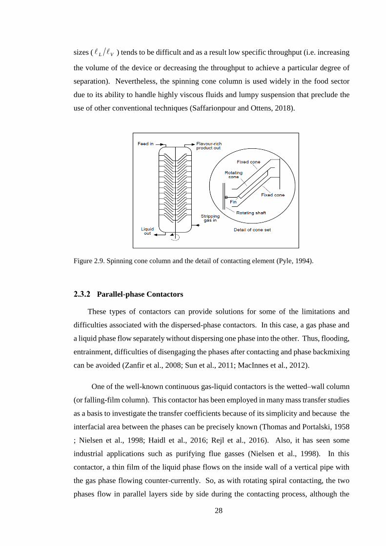
28
sizes ( ) tends to be difficult and as a result low specific throughput (i.e. increasing
the volume of the device or decreasing the throughput to achieve a particular degree of
separation). Nevertheless, the spinning cone column is used widely in the food sector
due to its ability to handle highly viscous fluids and lumpy suspension that preclude the
use of other conventional techniques (Saffarionpour and Ottens, 2018).
Figure 2.9. Spinning cone column and the detail of contacting element (Pyle, 1994).
Parallel-phase Contactors
These types of contactors can provide solutions for some of the limitations and
difficulties associated with the dispersed-phase contactors. In this case, a gas phase and
a liquid phase flow separately without dispersing one phase into the other. Thus, flooding,
entrainment, difficulties of disengaging the phases after contacting and phase backmixing
can be avoided (Zanfir et al., 2008; Sun et al., 2011; MacInnes et al., 2012).
One of the well-known continuous gas-liquid contactors is the wetted–wall column
(or falling-film column). This contactor has been employed in many mass transfer studies
as a basis to investigate the transfer coefficients because of its simplicity and because the
interfacial area between the phases can be precisely known (Thomas and Portalski, 1958
; Nielsen et al., 1998; Haidl et al., 2016; Rejl et al., 2016). Also, it has seen some
industrial applications such as purifying flue gasses (Nielsen et al., 1998). In this
contactor, a thin film of the liquid phase flows on the inside wall of a vertical pipe with
the gas phase flowing counter-currently. So, as with rotating spiral contacting, the two
phases flow in parallel layers side by side during the contacting process, although the
VL

29
liquid layer thickness cannot be decoupled from the liquid phase flow rate in this case
since gravity cannot be changed. Thus, increasing or decreasing the liquid phase flow
rate will lead, necessarily, to increasing or decreasing the liquid layer thickness. Further,
the stability of the phase interface is crucial for this type of contacting. Effective parallel-
phase contacting relies on maintaining the phases separated with phase interface
remaining stable (Hessel et al., 2005; Lam et al., 2013; MacInnes et al, 2012). Disrupting
this organised flow potentially results in changing phase layer thicknesses (VL ) or
even breaking up the interface into droplets or bubbles and hence uncontrolled contacting.
In the wetted-wall column, obtaining unstable flow is highly possible. Operating at large
velocity of one of the phases produces a wavy flow, making the contacting more complex
and uncontrolled (Boomkamp and Miesen, 1996 ; Nielsen et al., 1998).
The falling film microcontactor is a novel approach developed last decade as an
alternative to improve gas-liquid contacting in the wetted-wall column and other
conventional approaches (Monnier et al., 2010). This contactor typically consists of a
number of straight microchannels extended vertically on a plate (Fig. 2.10). The laminar
nature of fluid flow in these channels and their small size result in a flow dominated by
surface forces. This helps to stabilise the liquid layer during the contacting process (Lam
et al., 2013). Also, using microchannels provides a high surface area per unit volume and
hence better contacting can be achieved in relation to the conventional wetted-wall
column (Hessel et al., 2005). However, controlling the liquid layer thickness is still not
within the capability of this approach since the liquid phase flows under the effect of
gravity. Also, gravity is weak to counter the large surface forces which result sometimes
in segmented flow rather than continuous flow (Aota et al., 2009), eliminating the benefit
of counter-current contacting. Thus, it should be expected that the use of gravity to drive
the liquid phase in such small channels can limit the allowable phase flow rates.
Additionally, liquids with a large contact angle may not wet the channel completely,
causing liquid maldistribution (Al-Rawashdeh et al., 2008). This adversely affects the
mass transfer by decreasing the amount of the interfacial area.
A number of studies in the literature investigated the process of gas-liquid contacting
in falling film microcontactors. Most of the attention in these studies is on co-current and
counter-current chemical absorption, in particular the absorption of CO2 using NaOH
solution (Zanfir et al., 2005; Al-Rawashdeh et al., 2008; Ziegenbalg et al., 2010 ; Al-

30
Rawashdeh et al., 2012, reviewed by Lam et al., 2013). Relatively few studies focus on
physical mass transfer. Monnier et al. (2010) demonstrate counter-current absorption of
tetrachloroethylene from air into diethylhexyladipate using a falling film microcontactor.
The authors compare the separation efficiency (measured based on the degree of
purification) with results of a conventional packed bed for the same phase and solute
system. The results were comparable, although an excessive amount of the
solvent was used for the packed bed, i.e. )1(1 Vn aqf −− , in relation to the fall film
microcontactor to achieve the same degree of separation. Furthermore, a theoretical study
has been carried out by Mhiri et al. (2011). The authors analysed the gas-liquid contacting
process in the same apparatus of Monnier et al. (2010) using the same phase and solute
system. They looked at the effect of the gas layer thickness and they found that a good
improvement in mass transfer can be achieved by decreasing the gas layer thickness. This
improvement was attributed to the role of .f The system studied by Monnier et al.
(2010) and Mhiri et al. (2011) has a small f , which means that the solute is very soluble
in the liquid phase. Hence, decreasing the gas layer thickness resulted in an improvement
in mass transfer since most of the mass resistance lies in the gas-side.
Figure 2.10. A falling film microcontactor developed by Institut für Mikrotechnik Mainz and
its expanded view (adapted from Monnier et al., 2010).

31
A further, rather different, method of continuous gas-liquid contacting employs a
membrane barrier. The membrane, essentially, acts as a means of allowing a gas and a
liquid phase to contact in small pores distributed inside it (Mahmud et al., 1998; Simons,
et al., 2009). Unlike the wetted-wall column, this method of contacting enables the phase
element sizes ( ) to be independent of the phase flow rates, providing a constant
and high specific interfacial area (Zanfir et al., 2008). But equally, these elements are
fixed and cannot be adjusted since they are determined by the contactor internal design
(the size of the fluid passages and the membrane configuration). So a design suitable for
one phase and solute system may not be suitable for others. Further, a solute species
needs to diffuse through the membrane to transfer between the phases. This means that
there is an additional mass transfer resistance created by the membrane which will reduce
the mass transfer effectiveness. Another important point is that handling completely
wetting liquids can be problematic. Such liquids pass easily through the membrane pores
into the gas side, reducing in this way the contacting efficiency. There are also other
operational issues inherent in membrane contactors such as fouling, which strongly
affects mass transfer performance, and a limited membrane lifespan (Gabelman and
Hwang, 1999; Zanfir et al., 2008; Sun et al., 2011).
Recently, a mesh microcontactor has been developed to minimise membrane
limitations (Wenn et al., 2003; Zanfir et al., 2008). This contactor is based on using a
mesh with straight micropores distributed in a regular and organised manner (Fig. 2.10).
This micromesh provides less resistance, higher porosity and more organised pore
structure comparing to membrane (Zanfir et al., 2008; Sun et al., 2011). On the downside,
however, using a thin mesh with large pore size increases the possibility of breakthrough
of one phase into the other (Lam et al., 2013). Thus, precise control of the operating
conditions, especially the difference of pressure between phases, is required to avoid such
phase intermixing (Zanfir et al., 2008 ; Sun et al., 2011).
A number of studies have been conducted using the mesh microcontactor in various
separation applications. Some of these studies focused on co-current physical desorption
(Zanfir et al., 2008; Sun et al., 2011; Constantinou et al., 2014). Counter-current
desorption is reported in Cypes and Engstrom (2004) and Chasanis et al. (2011). Both
groups investigated stripping of toluene from water into a nitrogen stream. It was shown
in both studies that the overall coefficient obtained is higher by up to two orders of
VL

32
magnitude than that of a conventional packed column treating the same phase and solute.
Different than these studies, Adiche (2018) recently reported desorption of acetone-
water-N2 system using a hydrophobic/oleophobic membrane microcontactor based on
two meandering channels. The author investigated the effect of the liquid channel depth
and hence the liquid layer thickness on the stripping efficiency over a range of phase flow
rate ratios. The results showed that the smaller the channel depth, the higher is the mass
transfer over the tested range of phase flow. Finally, as the falling film microcontactor,
there are some studies that focus on the co-current chemical absorption of CO2 using
NaOH solution (Constantinou and Gavriilidis, 2010; Constantinou et al., 2012).
Figure 2.11. Schematic diagram showing the principle of contacting in a mesh microcontactor
(Lam et al., 2013).
Rotating Spiral Technique
An Overview of Attempts to Use Rotating Spiral
A considerable number of patents have been granted concerning the exploitation of
centrifugal acceleration in separation processes. However, a survey of these reveals that
the concept of rotating spiral contacting only appears in the earliest patents of
Podbielniak in the 1930s (Podbielniak 1935, 1936, 1937, 1938). In these patents, the
rotating spiral technique was presented as a promising approach capable of handling gas-
liquid and liquid-liquid counter-current separations. Podbielniak and his co-workers were
the first to develop commercially a rotating device for separation (extraction) in 1947
(Trent, 2003; Coulson et al., 2002). Different forms of rotating contacting element have
been proposed by this group; the original design of a spiral element was apparently soon
replaced by a perforated spiral and then, for reasons related to design flexibility and ease
of manufacturing, with perforated concentric shells (Todd and Podbielniak, 1965).

33
Of these proposed contacting elements, only the final version of modifications found
its way to commercial use in penicillin extraction (Podbielniak et al., 1970), while the
original spiral design (non-perforated spiral) was never exploited. MacInnes and Zambri
(2015) attributed the dropping of the rotating spiral design to two main reasons,
which probably led to an unsuccessful operation. Firstly, all the proposed designs were
restricted to a horizontal axis orientation as shown in Fig. 2.12. This unfortunate choice
of operation allows the phase layer thicknesses to be crucially affected by gravity. The
centrifugal component along the spiral channel, the driving force of the heavy phase, is
strengthened by gravity at some positions and weakened by it at others, producing
variable layer thicknesses ( ). Secondly, using a large channel size indicates that
the operation was performed at large values of Reynolds numbers, which were probably
high enough to create interfacial instability and loss of control (MacInnes et al., 2012).
Figure 2.12. Podbielniak Contactor (Coulson et al., 2002).
Unrelated to the Podbielniak et al.’s work, the next investigation of rotating spiral
technique appears to be a theoretical study of Mochalova et al. (1973). The authors
looked at the hydrodynamic characteristics and the mass transfer performance in a
rotating spiral channel, considering a stable laminar flow. This modelling work was
extended by Zhavoronkov et al. (1977) to include the behaviour of flow and the mass
transfer rate at the entrance region of the spiral. In either case, the solution of the
governing equations of motion was approximated for the case of external flow over a
rotating spiral surface to find the liquid layer thickness and mass transfer coefficient in
the liquid side. Unfortunately, there is no indication in the literature that these theoretical
works were ever utilized or even compared with experimental work. Thus, the accuracy
of these models was not proved. However, approximating the solution to the case of
VL
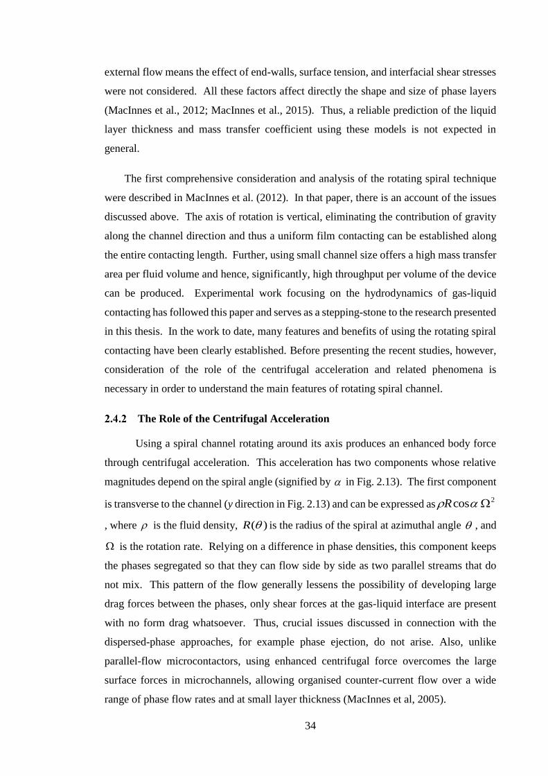
34
external flow means the effect of end-walls, surface tension, and interfacial shear stresses
were not considered. All these factors affect directly the shape and size of phase layers
(MacInnes et al., 2012; MacInnes et al., 2015). Thus, a reliable prediction of the liquid
layer thickness and mass transfer coefficient using these models is not expected in
general.
The first comprehensive consideration and analysis of the rotating spiral technique
were described in MacInnes et al. (2012). In that paper, there is an account of the issues
discussed above. The axis of rotation is vertical, eliminating the contribution of gravity
along the channel direction and thus a uniform film contacting can be established along
the entire contacting length. Further, using small channel size offers a high mass transfer
area per fluid volume and hence, significantly, high throughput per volume of the device
can be produced. Experimental work focusing on the hydrodynamics of gas-liquid
contacting has followed this paper and serves as a stepping-stone to the research presented
in this thesis. In the work to date, many features and benefits of using the rotating spiral
contacting have been clearly established. Before presenting the recent studies, however,
consideration of the role of the centrifugal acceleration and related phenomena is
necessary in order to understand the main features of rotating spiral channel.
The Role of the Centrifugal Acceleration
Using a spiral channel rotating around its axis produces an enhanced body force
through centrifugal acceleration. This acceleration has two components whose relative
magnitudes depend on the spiral angle (signified by in Fig. 2.13). The first component
is transverse to the channel (y direction in Fig. 2.13) and can be expressed as2cos R
, where is the fluid density, )(R is the radius of the spiral at azimuthal angle , and
is the rotation rate. Relying on a difference in phase densities, this component keeps
the phases segregated so that they can flow side by side as two parallel streams that do
not mix. This pattern of the flow generally lessens the possibility of developing large
drag forces between the phases, only shear forces at the gas-liquid interface are present
with no form drag whatsoever. Thus, crucial issues discussed in connection with the
dispersed-phase approaches, for example phase ejection, do not arise. Also, unlike
parallel-flow microcontactors, using enhanced centrifugal force overcomes the large
surface forces in microchannels, allowing organised counter-current flow over a wide
range of phase flow rates and at small layer thickness (MacInnes et al, 2005).

35
Figure 2.13. Rotating spiral contactor: geometric parameters and principle of operation.
The second component of centrifugal force acts along the channel (z direction in Fig.
2.13) and is 2sin R . This component acts on both the liquid and the gas phase,
affecting flows along the channel. Since the density of the liquid phase, in general, is
significantly larger than that for the gas phase, this component mainly affects the liquid
phase. It is employed to drive the liquid forward along the spiral while the gas phase can
travel counter-currently under the influence of pressure gradient. Thus, for a given phase
and solute system, the phase layer thickness ratio ( ) depends on the spiral
geometry (through sinR ), the rotation rate and the pressure gradient. The geometric
parameters of the Archimedean spiral, which is considered here, can be related by the
following polar equation (MacInnes et al., 2005; MacInnes et al., 2010):
( ) ( )( )
2
0th
RR+
+= (2.15)
where h and t (identified in Fig. 2.13) are the channel height and the distance between
adjacent revolutions, respectively.
For practical spirals, is small (MacInnes et al., 2012) and thus, the change in spiral
radius with can be expressed by:
= sin1
d
dR
R (2.16)
Noting that ( ) 2thddR += from Eq. 2.15, so sinR and hence the centrifugal
VL
)(R
th
Rotation
Axis
Spiral
Channel

36
force along the channel remains constant provided h and t are constant. This
corresponds to an Archimedean channel of fixed shape and size (Fig. 2.13). Thus, the
centrifugal body force remains constant along the channel and a large component is
applied in the transverse direction ( sincos RR ). This means that suitable
adjustment of the rotation rate and pressure gradient change and this ratio remains
uniform along the full length of spiral. Hence, in contrast to most available methods,
and LV QQ may be adjusted to the values that achieve optimum contacting and
this optimum prevails throughout the contacting process.
Further, this flexibility of controlling the phase flow rate and element sizes enables
a wide range of phase and solute systems to be within the capability of this technique. An
unpublished study carried out by MacInnes (2013) shows that a single channel design
with moderate adjustment of the pressure gradient and the rotation rate can operate at
flow rate ratios from 10-4 to 104 and handle liquid viscosities from 0.2 to 800 cP and
density ratios from 0.1 up to 0.99. As one may note, this easily encompasses the widest
conceivable range of possible practical phase and solute systems and required operating
conditions.
Coriolis Acceleration and Secondary Motion
The motion of fluids in a rotating channel is subject to Coriolis acceleration
that produces distinctive features in rotating flows (Barua, 1954; Benton, 1956). Coriolis
acceleration has the effect of a force which is perpendicular to both the direction
of the flow and the rotation vector (Tritton, 1988). For two phases flowing in a
rotating channel (Fig. 2.14) then, this force per unit volume can be expressed in each
phase as V
− 2 where is the phase density,
the rotation vector and V
the
velocity vector in the rotating reference frame (e.g. Speziale, 1982). It is clear from this
basic definition and the case depicted in Fig. 2.14 that there is no Coriolis effect in the
direction parallel to , whereas w2 and v− 2 (Fig. 2.14 a) are the remaining
Coriolis terms in y and z directions, respectively, in each phase. The direction of these
forces is determined merely by the direction of both the velocity and the rotation
vector. For counter-current contacting, positive rotation rate and negative v component,
therefore, one would expect that the direction of Coriolis terms is exactly as that shown
in Fig. 2.14 a.
VL
VL
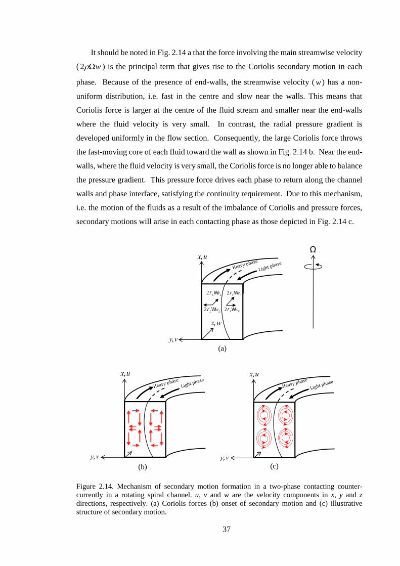
37
(a)
(c)(c)(b)
x,u
y,v
z,w
2rVWvV2rLWvL
2rLWwL 2rVWwV
Ω
(a)
x,u
y,v
x,u
y,v
(c)
It should be noted in Fig. 2.14 a that the force involving the main streamwise velocity
( w2 ) is the principal term that gives rise to the Coriolis secondary motion in each
phase. Because of the presence of end-walls, the streamwise velocity ( w ) has a non-
uniform distribution, i.e. fast in the centre and slow near the walls. This means that
Coriolis force is larger at the centre of the fluid stream and smaller near the end-walls
where the fluid velocity is very small. In contrast, the radial pressure gradient is
developed uniformly in the flow section. Consequently, the large Coriolis force throws
the fast-moving core of each fluid toward the wall as shown in Fig. 2.14 b. Near the end-
walls, where the fluid velocity is very small, the Coriolis force is no longer able to balance
the pressure gradient. This pressure force drives each phase to return along the channel
walls and phase interface, satisfying the continuity requirement. Due to this mechanism,
i.e. the motion of the fluids as a result of the imbalance of Coriolis and pressure forces,
secondary motions will arise in each contacting phase as those depicted in Fig. 2.14 c.
Figure 2.14. Mechanism of secondary motion formation in a two-phase contacting counter-
currently in a rotating spiral channel. u, v and w are the velocity components in x, y and z
directions, respectively. (a) Coriolis forces (b) onset of secondary motion and (c) illustrative
structure of secondary motion.
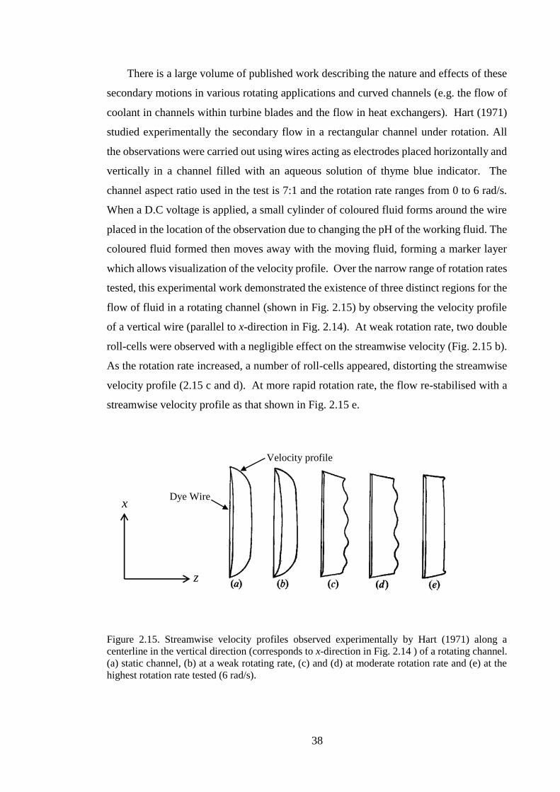
38
There is a large volume of published work describing the nature and effects of these
secondary motions in various rotating applications and curved channels (e.g. the flow of
coolant in channels within turbine blades and the flow in heat exchangers). Hart (1971)
studied experimentally the secondary flow in a rectangular channel under rotation. All
the observations were carried out using wires acting as electrodes placed horizontally and
vertically in a channel filled with an aqueous solution of thyme blue indicator. The
channel aspect ratio used in the test is 7:1 and the rotation rate ranges from 0 to 6 rad/s.
When a D.C voltage is applied, a small cylinder of coloured fluid forms around the wire
placed in the location of the observation due to changing the pH of the working fluid. The
coloured fluid formed then moves away with the moving fluid, forming a marker layer
which allows visualization of the velocity profile. Over the narrow range of rotation rates
tested, this experimental work demonstrated the existence of three distinct regions for the
flow of fluid in a rotating channel (shown in Fig. 2.15) by observing the velocity profile
of a vertical wire (parallel to x-direction in Fig. 2.14). At weak rotation rate, two double
roll-cells were observed with a negligible effect on the streamwise velocity (Fig. 2.15 b).
As the rotation rate increased, a number of roll-cells appeared, distorting the streamwise
velocity profile (2.15 c and d). At more rapid rotation rate, the flow re-stabilised with a
streamwise velocity profile as that shown in Fig. 2.15 e.
Figure 2.15. Streamwise velocity profiles observed experimentally by Hart (1971) along a
centerline in the vertical direction (corresponds to x-direction in Fig. 2.14 ) of a rotating channel.
(a) static channel, (b) at a weak rotating rate, (c) and (d) at moderate rotation rate and (e) at the
highest rotation rate tested (6 rad/s).
x
z
Dye Wire
Velocity profile

39
Speziale and Thangam (1983) computed the laminar flow of an incompressible fluid
(single-phase) in a large aspect-ratio rectangular channel (8:1). The results were in good
agreement with the experiments of Hart (1971). Both studies found that the critical point
at which the instability mode (Fig. 2.15 c and d) occurred is at a Reynolds number of
about 100 and Rossby number (Ro) of around 1. Ro is the ratio of the inertial force to the
Coriolis force and is expressed as DwB where Bw is the bulk streamwise velocity and
D is the channel width. Also, the computations of Speziale and Thangam (1983) showed
clearly that there is an appreciable distortion in the streamwise velocity profiles along the
transverse direction of the channel (corresponds to y-direction in Fig. 2.14) in relation to
the pure pressure driven flow in a static channel (Poiseuille flow). Such distortion was
confirmed by other computational studies made by Kheshgi and Scriven (1985) and Selmi
et al. (1994). The former studied the behaviour of laminar flow of a single phase in a
straight rotating channel, while the latter focused on the laminar flow in a curved channel
under rotation. Fig. 2.16 shows the pattern of the secondary motion and the corresponding
streamwise velocity profile computed by Selmi et al. (1994) at different Ro. The figure
shows clearly the change in the distortion pattern of the streamwise velocity (Figs. 2.16
b, d, f and h) as the secondary flow changes (Figs. 2.16 a, c, e and g) with Ro.
Numerical studies have also been carried out to investigate the flow analogy in
stationary curved ducts and rotating ducts (Lee and Baek 2001, 2002, 2006). For both
laminar and turbulent flow, the authors found that the secondary motion increases the
mean friction factor and they pointed out to that these secondary motions induce the heat
transfer rate. In terms of the mass transfer, Ikehata et al. (2004) studied the effect of
Coriolis force on the counter-current chromatographic separation by changing the
direction of column rotation (i.e. anticlockwise or clockwise). For all solvent systems
used, they found that there is a pronounced effect of Coriolis force on the performance of
separation. The results also show that the clockwise rotation considerably enhances the
separation performance with a lower retention time, irrespective of what the type of
mobile phase is.
Similarly, in the rotating spiral contacting, Coriolis secondary motion is present and
affects consequently the flow characteristics and mass transfer. As far as the author
knows, the role of this motion, its structure and how it affects the mass transfer process
in the spiral channel have not yet been explored. In this work, the effect of this secondary
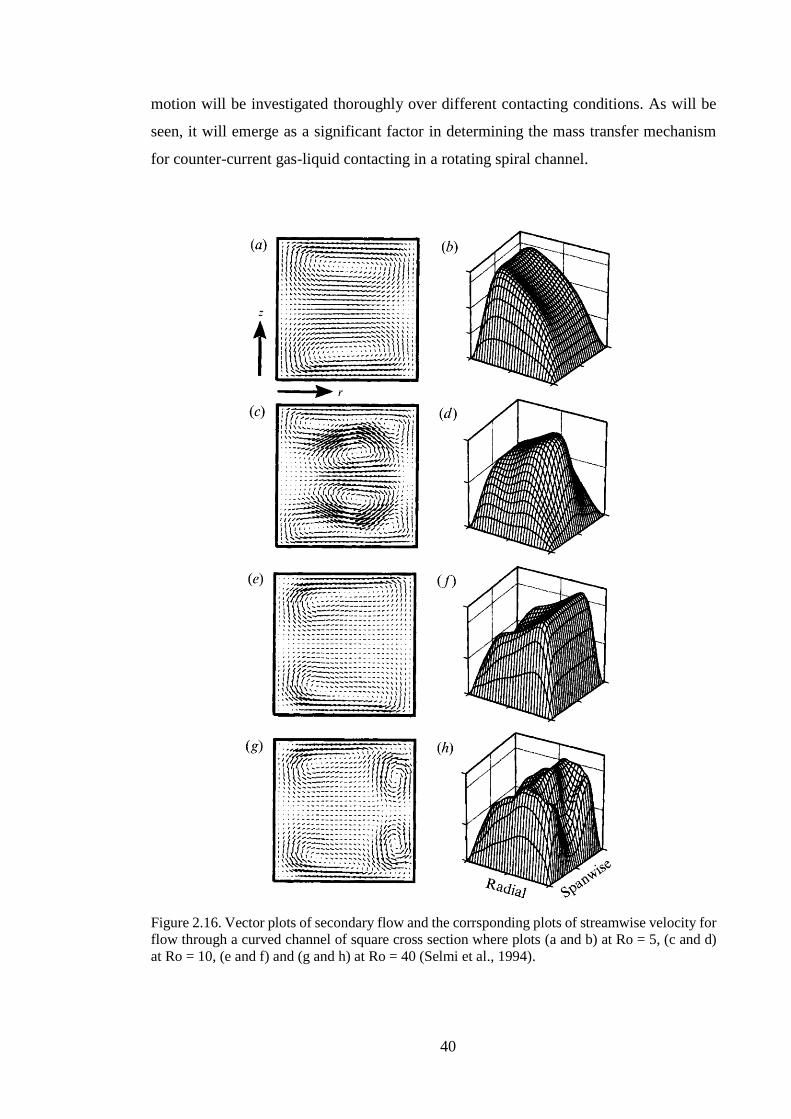
40
motion will be investigated thoroughly over different contacting conditions. As will be
seen, it will emerge as a significant factor in determining the mass transfer mechanism
for counter-current gas-liquid contacting in a rotating spiral channel.
Figure 2.16. Vector plots of secondary flow and the corrsponding plots of streamwise velocity for
flow through a curved channel of square cross section where plots (a and b) at Ro = 5, (c and d)
at Ro = 10, (e and f) and (g and h) at Ro = 40 (Selmi et al., 1994).

41
Recent Studies of the Rotating Spiral
A theoretical study of rotating spiral contacting was performed by MacInnes et al.
(2005). In the study, a hydrodynamic analysis was carried out for a vapour-liquid system
flowing counter-currently to explore the feasibility of this technique. It was found that
with minor changes to geometric parameters such as the channel angle, the pressure
gradient and the centrifugal force could be controlled to produce a suitable counter-
current flow.
Ortiz-Osorio et al. (2009) performed a numerical computation for a specific
experimental condition of a rotating spiral distillation reported later by MacInnes et al.
(2010). In the computation, the interface is assumed to be a perfect circle (Fig. 2.17).
Such assumption is likely acceptable since the channel has micro-dimensions, causing the
variation in the pressure across the interface to be negligible in relation to the surface
tension. The bulk concentration in the liquid and vapour phase was computed and the
results showed a good agreement with those measured experimentally.
Figure 2.17. The results of computation for two phases with a circular interface, (a) the main
velocity distribution, (b) the direction of the secondary motion (no magnitudes) and (c) the solute
concentration distribution (Ortiz-Osorio et al., 2009).
An experimental exploration of rotating spiral contacting has been performed by
MacInnes et al. (2010). In the study, a rotating apparatus was developed using a
spiral microchannel (Fig. 2.18) to conduct a stripping distillation. A binary mixture of
hydrocarbons (50:50 of 2,2-dimethylbutane and 2-methyl-2-butene ) was used as a
feedstock. The idea of bringing two immiscible phases (vapour-liquid) to flow side by
Liquid Phase
Vapour Phase

42
side counter-currently at micro-level was achieved successfully via this technology,
resulting in an efficient multiple stages distillation.
Figure 2.18. Spiral microchannel (255 95) µm2 formed into a glass chip.
Fig. 2.19 shows the components of the apparatus used. As can be seen, it is equipped
with a relatively large rotating unit. This unit holds all the main parts: the feed reservoir
(only its atmospheric vent shown in Fig. 2.19 a), the distillate and the bottom collecting
reservoirs (vials shown in Fig. 2.19 a), the spiral channel chip (not shown) and the
heating and cooling elements (Fig. 2.19 b). The work gives a detail description of the
temperature distribution and the flow network of the phases. These are crucial factors to
control the evaporation process to generate the second phase (vapour). As the feed travels
along the spiral channel, the temperature increases in a consistent manner such that
evaporation occurs beyond the junction region (Fig. 2.18). This evaporation creates a
pressure difference along the spiral which is enough to push the vapour phase backward
to oppose the liquid that is primarily driven by the centrifugal force.
The above work demonstrated experimentally the feasibility of this technique by
producing a distillation-like process. It was shown that a stable counter-current film
contacting could be achieved practically by adjusting both the rotation rate and pressure
drop along the channel.

43
Figure 2.19. The main parts of the apparatus: (a) top view of the rotating unit and (b) the bottom
view of the rotating unit.
Subsequently, a theoretical study has been reported in MacInnes et al. (2012). The
study included analysis and modelling of two-phase contacting in a rotating spiral
with infinite-width. As a result, an analytical model ‘wide-channel model’ was
developed. The solution of the model defines explicitly the relations between the
hydrodynamics parameters, transfer coefficients, spiral geometry and operating
conditions (pressure drop and rotation rate) in closed-formed expressions. In the work,
MacInnes et al. (2012) also proposed dimensionless parameters as a preliminary guide to
obtain a stable flow. Using the same notation identified in Figs. 2.13 and 2.14, the
minimum radial position of the spiral channel ( minR ) and the heavy phase volume fraction
( ), these parameters can be expressed as:
V
VBVV
hw
)1(Re
−=
L
LBLL
hw
=Re
hR
wLB
2
min
Fr
= ( )
hww VBLBV
2
We−
=
( )
22
minOE
hRVL −= 1
2
min
g
R
(2.17)
(b)
(a)

44
The first two ( VRe and LRe ) are Reynolds numbers in the two phases and must remain
less than some critical values to maintain steady and laminar flow. The third and fourth
parameters are Froude number ( Fr ) and Weber number ( We ), respectively. The former
can indicate where centrifugal body force waves at the phase interface may present. The
latter represents the tendency to form interfacial surface tension waves or to disintegrate
the interface into drops under high gas phase force. Each number must be less than some
critical value. The final two are Eötvös number ( OE ), here based on the centrifugal rather
than the gravitational acceleration, and the ratio of centrifugal and gravitational
acceleration ( gR 2
min ). These two constraints affect the interface shape. OE must be
large enough to overcome the surface forces which tend to confine the gas phase into
pockets surrounded by slugs of liquid phase, preventing ideal counter-current contacting.
2
minR , on the other hand, must be larger than g to ensure obtaining an interface parallel
to the channel walls and consequently phase layers of uniform thickness. These non-
dimensional numbers, along with the wide channel model, help to determine the
appropriate spiral dimensions and operating conditions under which stable interfacial
contacting can be achieved.
MacInnes and Zambi (2015) studied the hydrodynamics of gas-liquid contacting
using a newly developed apparatus. In contrast to the apparatus used in MacInnes et al.
(2010), this allows continuous, counter-current contacting of fluid phase over a wide
range of operating conditions. In the work, the variation of the liquid layer thickness
(measured at the minimum distance between the interface shape and the channel wall)
was examined as a function of phase flow rates, rotation rate and liquid viscosity. The
minimum liquid layer thickness and hence the interface position was traced by taking
digital images and analysing them using a model for the interface shape. The model was
verified in that same work by comparing to experimental results over a wide range of
conditions. Fig. 2.20 shows images taken to the phase layers at different conditions. In
each image, there are three distinct regions: air on the left side, water on the right side
and in between (grey region) the light reflected from the interface. Any changes in the
position or shape of the interface with the conditions appear in Fig. 2.20 as changes in the
grey region (interface region).

45
Figure 2.20. Images showing the phase layer thicknesses and meniscus size at different operating
conditions (Zambri, 2014). The images are taken from the bottom of the channel which
corresponds to the plane y-z in Fig. 2.14.
As expected, the authors found that by changing the rotation rate or the phase flow
rates, the position of the interface could be adjusted as required. For the changes of the
rotation rate (Fig. 2.20 a), they noticed that increasing the rotation rate at constant phase
flow rates decreases the liquid layer thickness and also decreases both the interface tilt

46
and the meniscus height at the end-walls. Also, they found that increasing the flow rate
of the liquid phase increases the liquid layer thickness as shown in Fig. 2.20 b. On the
other hand, the results showed that the effect of the gas phase flow rate is minor at high
rotation rate (Figs. 2.20 c) but becomes more pronounced at low rotation rate (2.20 d).
Additionally, liquids with a considerable range of viscosities (from about 0.6 to 60 cP)
were tested in that same work. The results showed that at constant rotation rate (3200
rpm), gas pressure (2.1 bar) and gas phase flow rate (1.15 NL/min), the liquid layer
thickness increases with increasing the liquid viscosity.
Recently, chemical counter-current absorption of carbon dioxide from nitrogen using
aqueous mixtures of diethanolamine (DEA) was investigated by MacInnes et al. (2017).
The work demonstrated the use of the rotating spiral as a rapid and accurate tool to
determine the optimum amine-water composition. This was made by comparing the
amount of the gas phase treated by different DEA compositions under conditions where
the liquid layer thickness is fixed (86 µm) and 90% removal of CO2 is required. The
study found that a DEA mass fraction of about 31% gave a maximum gas phase
throughput at the required degree of purification.
This Research
The current work is linked strongly to the previously described works on the rotating
spiral and is designed to build on systematically. The most crucial outcome emerging
from the studies presented is that a full theoretical treatment of rotating spiral contacting
is possible. This conclusion opens up the way to establish a general modelling approach
to two phase contacting in a rotating spiral channel. The approach is based on a
combination of the interface shape model (MacInnes and Zambri, 2015) and the 2-D
governing equations. This helps to simulate the process of contacting, using the actual
shape of the interface and including the Coriolis acceleration. In this way, the details of
the flow and species fields can be calculated under different contacting conditions,
opening up the possibility of deeply understanding the mass transfer process in rotating
spiral channel which is one of the main aims here.
The work also includes an extensive experimental investigation of physical mass
transfer (desorption) in a rotating spiral channel. These experiments aimed to study and
understand the characteristics of the physical mass transfer in this novel contactor over

47
different phase flow rates. It has been argued in this chapter that the rotating spiral,
uniquely, possesses the characteristics of producing improved contacting: independent
control of the phase element length scales and phase flow rates. Quantifying this
improvement is a significant step. Therefore, another direction here is to use the
experimental results obtained to quantify the performance of the spiral in relation to
alternative contacting approaches. For this purpose, a theoretical framework that allows
a comparison between different approaches is developed and given in Chapter 3. The
mass transfer results are also used to test critically the 2-D numerical model adopted in
this work, determining its limitations. The theory behind the model is given in Chapter 4
while the comparison with the experimental data is discussed in Chapter 8, after
presenting the experimental work (Chapter 5), determining the required physical
properties (Chapter 6) and characterising the mass transfer behaviour using the
experimental results (Chapter 7).

48
Chapter Three
3 Bulk Mass Transfer Analysis and Basic Relations
The previous chapter discusses gas-liquid contacting including the most common
types of contactors and highlights features of rotating spiral channel. For most of these
contactors a simple mass transfer analysis for a solute being transfer between the two
immiscible phases is possible. Such analysis can be applied for both co-current and
counter-current contacting, whether the process is absorption or desorption and whether
the flow is linear or radial such as for rotating packed bed. In either case, ordinary
differential equations based on the bulk quantities of the phases and transfer coefficients
govern the mass transfer. Useful relations can be derived from the solution of
these equations, linking the measurable inlet and outlet solute concentrations (bulk) to
mass transfer coefficients. Therefore, it is possible to gain insight into the mass transfer
performance at any contacting condition of interest. Also, the derived relations can be
used to analyse results for any contacting method. So they can be employed as a basis
for comparing different contacting devices. This can be done regardless of solute
properties and operating conditions, allowing direct comparison between the rotating
spiral and other contactors performing similar separation task.
This chapter gives a full presentation of the bulk mass transfer analysis and the
resulting relations. As in the experiments in this work, attention is focused on counter-
current contacting and the case of dilute solute. Counter-current flow enables an unlimited
number of equilibrium stages to be reached and hence a high degree of purification. The
case of a dilute solute ensures constant physical properties in each phase and linear
representation of the solute equilibrium curve. Further, a broad range of applications
involve the purification of dilute solute, such as removal of organic compounds or other
trace toxics from waste water (Hartwick and Howat, 1995; Sherman et al., 1996).
Relations for determining the mass transfer coefficients are developed first. These
relations lead to a useful design equation which links purification with the phase flow
rates ratio, the residence time of the processed phase and the contacting effectiveness.
The contacting effectiveness is represented here by the specific throughput which is the
volumetric flow rate of the processed phase per volume of one equilibrium stage

49
dz0 L
z
Heavy
PhaseLight
Phase
fb
a ,
fP
(MacInnes et al, 2012). Another important parameter introduced is the total specific
throughput, which is the specific throughput divided by the number of stages required to
achieve a given purification. This parameter is used in this work to compare the rotating
spiral channel with other alternative approaches over a range of solute properties and
contacting conditions as discussed in Chapter 7.
3.1 Counter-current Contacting Analysis
A general state of counter-current fluid-phase contacting in a contactor with length
L is depicted in Fig. 3.1 where the notation a and are the interfacial area per unit
volume of the passage and the volume fraction occupied by the heavy phase, respectively.
To give a general context and simplify the discussion, the gas phase is referred to as the
‘light’ phase with subscript ‘V ’ and the term ’heavy’ phase with subscript ‘ L ‘ is used to
designate the liquid phase.
Figure 3.1. Counter-current contacting of two phases over length L produced by a suitable
magnitude of body force ( bf ) and pressure force ( pf ).
The flow of the phases in Fig. 3.1 is in the direction of the z-coordinate. When a
body force per unit volume ( bf ) acts in the positive z-direction and a pressure force
( pf ) acts in the negative z-direction, a counter-current mode of flow is possible. In this
case, the heavy phase, represented by dispersed droplets, travels in the direction of the
body force since it has a larger density while the light continuous phase flows in the
opposite direction. Similarly, co-current flow may occur in either direction along z. Both
phases can flow in the positive direction when the body force is dominant or in the
negative direction when the pressure force is sufficiently large. It is also possible for the
heavy phase to be the continuous phase, e.g. in bubble columns, or both phases could be
continuous as the case for rotating spiral and falling film contactors. All these possible
cases are described in Chapter 2 and they do not change the analysis in this chapter.

50
The mass transfer experiments performed in this work consider desorption in which
the solute transfers from the liquid to the gas phase. Accordingly, a differential mole
balance for a solute being desorbed from the heavy phase into the light phase over a region
of dz length (Fig. 3.1) can be expressed as:
Heavy phase: ajdz
YwndL
LBLBL =− )(
(3.1)
Light phase: ajdz
YwndV
VBVBV =− ))1((
(3.2)
where Vn and Ln are the phase molar densities , VBw and LBw are the bulk velocities
with VBw negative according to the coordinates used in Fig. 3.1, VBY and LBY are the bulk
solute mole fractions and Vj and Lj are the solute molar flux transferred across the phase
interface based on the two phases.
The flux in Eqs. 3.1 and 3.2 may be expressed in terms of two individual mass
transfer coefficients ( Vk and Lk ) and the difference between the bulk solute mole fractions
and those at the interface ( VIY and LIY ):
Heavy phase: )( LILBLL YYkj −= (3.3)
Light phase: )( VBVIVV YYkj −= (3.4)
Substituting Eqs. 3.3 and 3.4 in Eqs. 3.1 and 3.2, respectively, gives:
Heavy phase: )()(
LILBLLBLBL YYak
dz
Ywnd−=
− (3.5)
Light phase: )())1((
VBVIVVBVBV YYak
dz
Ywnd−=
− (3.6)
The derivatives on the left hand sides of the above equations can be expanded as:
dz
wndY
dz
dYwn
dz
Ywnd LBLLB
LBLBL
LBLBL )()(
−+−=
−
(3.7)
dz
wndY
dz
dYwn
dz
Ywnd VBVVB
VBVBV
VBVBV ))1(()1(
))1((
−+−=
−
(3.8)
The change in phase molar flow rates appeared in Eqs. 3.7 and 3.8 equals the amount of
solute being transferred, i.e.:

51
In Eq. 3.7: )()(
LILBLLBL YYak
dz
wnd−=
− (3.9)
In Eq. 3.8: )())1((
VBVIVVBV YYakdz
wnd−=
− (3.10)
Combining Eqs. 3.7, 3.8, 3.9 and 3.10 and substituting for the derivatives in Eqs. 3.5 and
3.6, give:
Heavy phase: )()1(
LILBLLB
LB
LBL YYakdz
dY
Y
wn−=
−
− (3.11)
Light phase: )()1(
)1(VBVIV
VB
VB
VBV YYakdz
dY
Y
wn−=
−
− (3.12)
Eqs. 3.11 and 3.12 give the variation of the bulk mole fraction in each phase in terms of
the individual mass transfer coefficients, specific interfacial area, bulk and interfacial
mole fractions and phase molar flow rates per unit area. The factors )1( LBY− and
)1( VBY− in these equations account for the change in molar flow rates due to changing
bulk mole fractions along the contacting length as a result of solute transport.
3.2 Overall Coefficients
The difficulty in using Eqs. 3.11 and 3.12 to analyse experiments directly centres
around the problem of knowing solute mole fractions at the interface ( LIY and VIY ). This
makes an analysis based on the individual coefficients impractical. By using ‘overall’
mass transfer coefficients, the flux (the right-hand terms in Eqs. 3.11 and 3.12) can be
expressed equivalently in terms of the bulk mole fractions in the two phases, eliminating
the need to determine LIY and VIY :
Heavy phase: )()( *
LBLBLLILBL YYKYYk −=− (3.13)
Light phase: )()( *
VBVBVVBVIV YYKYYk −=− (3.14)
where LK and VK are the overall mass transfer coefficients, *
LBY is a hypothetical solute
mole fraction that would be in equilibrium with that in the gas phase and *
VBY is similar
to *
LBY but in equilibrium with the liquid phase composition. The concept of these
hypothetical mole fractions ( *
LBY and *
VBY ) stems from the fact that mass transfer occurs

52
due to a departure from the equilibrium (i.e. *
LBLB YY − ). Thus, one might expect that if
the light phase becomes fully saturated with solute, LBY will be exactly *
LBY and hence the
net solute flux is zero. In practice, approaching such equilibrium case should be avoided
by choosing appropriate phase flow rates ratio, as discussed in Chapter 2, if a convenient
degree of purification is required.
Locally, the overall mass transfer coefficients can be expressed purely in terms of
the individual coefficients and the slopes of the equilibrium curve. In almost all
situations, this can be done under three conditions. First of all, the interface must be an
extremely thin layer without any contaminants or extra layers which might add resistance.
In this case, the interface does not store mass and equilibrium exists between LIY and
.VIY Second, there are no interfacial ripples or turbulence which can affect the individual
mass transfer coefficients. Third, the transfer of the solute across the interface is not
associated with chemical reaction (Sherwood et al., 1975). Under these conditions, the
interfacial mole fractions ( LIY and VIY ) lie on the solute equilibrium curve, ( )LBVB YfY =
, as shown in Fig. 3.2.
Figure 3.2. Graphical representation showing the relation between the local slopes of the
equilibrium curve and the bulk solute mole fractions in the light and heavy phase.
In the figure, ( LBY , VBY ) is any local position along the contacting length and 1f and 2f
are the local slopes of the equilibrium curve. These slopes can be determined graphically
using the values of the solute mole fractions ( LBY , VBY , LIY and VIY ):

53
LILB
VIVB
YY
YYf
−
−=
*
1 (3.15)
*2
LBLI
VBVI
YY
YYf
−
−= (3.16)
Using Eqs. 3.13 and 3.14, the solute mole fractions in Eqs. 3.15 and 3.16 can be replaced
by the transfer coefficients,
1fk
k
K
k
V
L
V
L += (3.17)
L
V
L
V
k
k
fK
k+
=
2
1 (3.18)
From Eqs. 3.17 and 3.18, it is clear that the local mass transfer coefficients can
be expressed in terms of the individual mass transfer coefficients and the slopes
of the equilibrium curve. However, these relations can only be used when a linear
representation of equilibrium curve is feasible.
To this point, the governing equations (Eqs. 3.11 and 3.12) can be expressed in terms
of the overall mass transfer coefficients using Eqs. 3.13 and 3.14:
Heavy phase: ( )LBLBLBLLB
LBL YYYaKdz
dYwn −−=− 1)( * (3.19)
Light phase: )1)(()1( *
VBVBVBVVB
VBV YYYaKdz
dYwn −−=− (3.20)
These differential equations are non-linear and must be solved by integrating along the
contacting length from the inlet to the outlet:
Heavy phase:
−−
−=
)(
)0(
*
0))(1(
LY
Y LBLBLB
LB
L
LBL
L LB
LBYYY
dY
aK
wndz
(3.21)
Light phase:
−−
−=
)(
)0(
*
0))(1(
)1(LY
Y VBVBVB
VB
V
VBV
L VB
VBYYY
dY
aK
wndz
(3.22)
In general, the integration requires numerical or graphical evaluation, i.e. evaluation of
the integrands over the relevant range of mole fractions. However, a full analytical
solution is possible with further approximation and that will be discussed in the next
section.
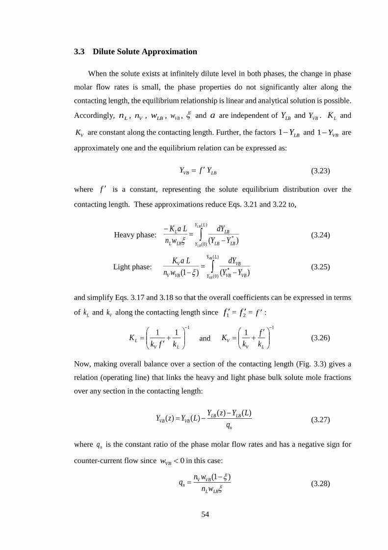
54
3.3 Dilute Solute Approximation
When the solute exists at infinitely dilute level in both phases, the change in phase
molar flow rates is small, the phase properties do not significantly alter along the
contacting length, the equilibrium relationship is linear and analytical solution is possible.
Accordingly, Ln , Vn , LBw , VBw , and a are independent of LBY and VBY . LK and
VK are constant along the contacting length. Further, the factors LBY−1 and VBY−1 are
approximately one and the equilibrium relation can be expressed as:
LBVB YfY = (3.23)
where is a constant, representing the solute equilibrium distribution over the
contacting length. These approximations reduce Eqs. 3.21 and 3.22 to,
Heavy phase: −=
−)(
)0(
* )(
LY
Y LBLB
LB
LBL
L
LB
LBYY
dY
wn
LaK
(3.24)
Light phase: −=
−
)(
)0(
* )()1(
LY
Y VBVB
VB
VBV
V
VB
VBYY
dY
wn
LaK
(3.25)
and simplify Eqs. 3.17 and 3.18 so that the overall coefficients can be expressed in terms
of Lk and Vk along the contacting length since 1f = 2f = f :
1
11−
+
=
LV
Lkfk
K and
1
1−
+=
LV
Vk
f
kK (3.26)
Now, making overall balance over a section of the contacting length (Fig. 3.3) gives a
relation (operating line) that links the heavy and light phase bulk solute mole fractions
over any section in the contacting length:
n
LBLBVBVB
q
LYzYLYzY
)()()()(
−−= (3.27)
where nq is the constant ratio of the phase molar flow rates and has a negative sign for
counter-current flow since 0VBw in this case:
LBL
VBVn
wn
wnq
)1( −= (3.28)
f

55
)(zYLB
L
)(zYVB )(LYVB
)(LYLB
Figure 3.3. A section of contacting length.
Since both Eqs. 3.23 and 3.27 are linear relations between LBY and VBY , the difference in
concentration (i.e. *
LBLB YY − and VBVB YY −* in Fig. 3.2) must also be linear with LBY and
VBY , thus:
)( *
LBLBLB YYddY − and )( *
VBVBVB YYddY − (3.29)
Using the abbreviations *
LBLBLB YYY −= and VBVBVB YYY −= * , Eq. 3.29 gives:
( ) ( )( ) ( )0
0
LBLB
LBLB
LB
LB
YLY
YLY
dY
Yd
−
−=
(3.30)
( ) ( )( ) ( )0
0
VBVB
VBVB
VB
VB
YLY
YLY
dY
Yd
−
−=
(3.31)
So, the integrals in Eqs. 3.24 and 3.25 may be expressed in terms of the variables LBY
and VBY and integrated to give two relations in terms aKL and aKV (e.g. Sherwood et
al., 1975):
( ) ( )
LB
LBLB
LBL
L
Y
YLY
wn
LaK
−=
− 0
(3.32)
( )
( ) ( )
VB
VBVB
VBV
V
Y
YLY
wn
LaK
−=
−
0
1 (3.33)
where ( ) ( )
( ) ( ) 0ln
0
LBLB
LBLBLB
YLY
YLYY
−= (3.34)
and ( ) ( )
( ) ( ) 0ln
0
VBVB
VBVBVB
YLY
YLYY
−= (3.35)
It is helpful to note here that
LBY and
VBY in the expressions for LBY and VBY are
linked to the solute mole fraction in each phase through the equilibrium relation (Eq. 3.23)
and can be expressed as fYY VBLB= and LBVB YfY = .

56
Now, Eqs. 3.32 to 3.35 can be used directly to determine aKL and aKV from the
inlet and outlet solute mole fractions for each phase, phase flow rates and equilibrium
constant. In practice, these parameters either can be measured directly such as the solute
mole fractions and the phase flow rates or estimated from the contacting conditions such
as , allowing a determination of the experimental aKL and aKV values.
3.4 Mass Transfer Performance
For fluid-fluid contacting, the mass transfer relies on two essential factors: the phase
flow rate ratio, which is represented by the purification factor ( nqf − ), and the phase
contacting effectiveness. The first is important to make ensure that a sufficient amount
of solvent is used to achieve the required degree of purification. The constraint on this
factor has been discussed in Chapter 2 (Section 2.2.1). For desorption, for example,
nqf − must satisfy the limit Ln dqf −− 1 (Eq. 2.7) where )0()( LBLBL YLYd = according
to the notations in Fig. 3.1. The contacting effectiveness, on the other hand, depends on
the way that the two phases are brought together in each particular contactor. In literature,
there are different measures that quantify this factor. The overall mass transfer coefficient
is the usual measure. Another measure is the length of a “transfer unit” based on one of
the phases (Anvaripour et al., 1995). It has a unit of length and represents the inverse of
the terms multiplying L on the right-hand side of Eqs. 3.33 and 3.34 (i.e. aKwn LLBL / or
aKwn VVBV /)1( − ). Equivalently, the specific throughput ( ) measures the
contacting effectiveness and will be used here. This term represents the volumetric flow
rate of fluid to be processed per passage volume corresponding to one equilibrium stage
(MacInnes, et al., 2012), i.e.:
(3.36)
The equilibrium stage is taken to have a contacting length of e which is required for the
exiting phases to have a solute composition corresponding to equilibrium. Using the
equilibrium stage concept, the length of a contactor then can be expressed as:
eeNL = (3.37)
where eN is the number of equilibrium stages.
f

57
For any contacting task, when a suitable phase flow rates ratio is selected
( Ln dqf −− 1 ), the required degree of separation ( ) determines eN and hence the
total passage length from Eq. 3.37 once e has been determined. The number of
equilibrium stages in Eq. 3.37, therefore, is simply a multiplicative factor, independent of
the contacting effectiveness. Hence, in a qualitative sense, a larger specific throughput at
a given value of nqf − indicates that larger volumetric flow rate of the process stream
can be treated in a given size of contactor ( L ) and degree of separation ( ). Specific
throughput also can be defined as the inverse of the processing time needed to accomplish
one equilibrium stage. Its reciprocal measures the passage volume required for each
equilibrium stage per unit volumetric flow rate of the process phase. Thus, the larger the
specific throughput at a given value of nqf − and (which fix eN ) the smaller e and
hence contactor size needed (Eq. 3.37) to purify a given throughput of the processed
phase.
Specific Throughput
The basic definition of the specific throughput given in Eq. 3.36 may be expressed
in terms of the heavy phase flow rate (process stream in desorption) which is AwLB and
the passage volume based on one equilibrium stage ( Ae ) as:
e
LB
e
LBL
w
A
Aw
== (3.38)
where A is the passage cross sectional area of a contactor.
For continuous, differential-contacting where there are no physically distinguishable
stages, e is an arbitrary length for which the contacting phases are at equilibrium.
Eq. 3.24 can be used directly to determine this arbitrary length by taking its position to
be z = 0 along the contacting and replacing L by e as:
−
−=
)(
)0(
* )(
eLB
LB
Y
Y LBLB
LB
L
LBLe
YY
dY
aK
wn
(3.39)
The integral term in Eq. 3.39 can be handled in the same manner used for Eq. 3.24 and
this gives:
Ld
Ld
Ld

58
)0()(ln)0()(
)()0(LBeLB
LBeLB
eLBLB
L
LBLe YY
YY
YY
aK
wn
−
−=
(3.40)
Using the general mole balance relation (Eq. 3.27) and setting z = 0 and eL = , the
relation between the heavy and light phase bulk solute mole fractions over the equilibrium
length may be given as:
n
eLBLBeVBVB
q
YYYY
)()0()()0(
−−=
(3.41)
Using the above equation and the fact that )0(VBY = )( eLBYf , Eq. 3.40 may be
simplified to:
( )
( )n
nn
L
LBLe
qf
qfqf
aK
wn
+
−=
1
ln (3.42)
Substituting Eq. 3.42 in 3.38, the corresponding relation for the specific throughput is:
( )
( )nn
n
L
LL
qfqf
qf
n
aK
−
+=
ln
1 (3.43)
This relation allows the calculation of the specific throughput from the overall mass
transfer coefficient, the molar density of the heavy phase and the purification factor
( nqf − ).
Total Specific Throughput
While the specific throughput is useful to judge the contacting effectiveness at
a particular nqf − , it becomes imprecise when different contacting conditions from
different equipment are involved. In this case, the purification factor ( nqf − ), the degree
of purification ( ), the throughput achieved and the size of the contactor used to achieve
the throughput must be considered. Comparison considering these factors needs to look
at the throughput per volume of the total passage required to achieve a specific purity.
This ‘total’ specific throughput, LN , differs from L precisely by the number of the
equilibrium stages required, i.e.:
e
L
ee
LBLBLN
NN
w
L
w ===
(3.44)
Ld
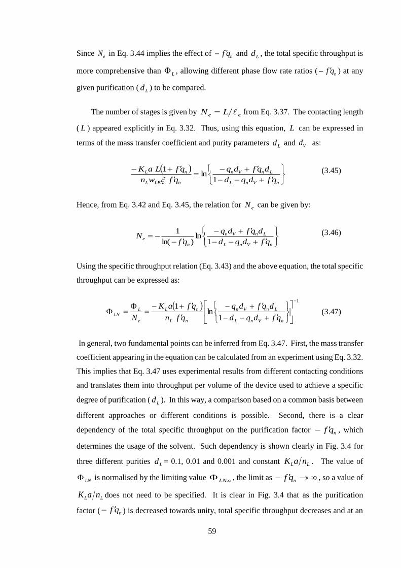
59
nqf −
Since eN in Eq. 3.44 implies the effect of nqf − and , the total specific throughput is
more comprehensive than L , allowing different phase flow rate ratios ( nqf − ) at any
given purification ( ) to be compared.
The number of stages is given by ee LN = from Eq. 3.37. The contacting length
( L ) appeared explicitly in Eq. 3.32. Thus, using this equation, L can be expressed in
terms of the mass transfer coefficient and purity parameters and as:
( )
+−−
+−=
+−
nVnL
LnVn
nLBL
nL
qfdqd
dqfdq
qfwn
qfLaK
1ln
1
(3.45)
Hence, from Eq. 3.42 and Eq. 3.45, the relation for eN can be given by:
+−−
+−
−−=
nVnL
LnVn
n
eqfdqd
dqfdq
qfN
1ln
)ln(
1 (3.46)
Using the specific throughput relation (Eq. 3.43) and the above equation, the total specific
throughput can be expressed as:
( )
1
1ln
1−
+−−
+−
+−=
=
nVnL
LnVn
nL
nL
e
LLN
qfdqd
dqfdq
qfn
qfaK
N (3.47)
In general, two fundamental points can be inferred from Eq. 3.47. First, the mass transfer
coefficient appearing in the equation can be calculated from an experiment using Eq. 3.32.
This implies that Eq. 3.47 uses experimental results from different contacting conditions
and translates them into throughput per volume of the device used to achieve a specific
degree of purification ( ). In this way, a comparison based on a common basis between
different approaches or different conditions is possible. Second, there is a clear
dependency of the total specific throughput on the purification factor nqf − , which
determines the usage of the solvent. Such dependency is shown clearly in Fig. 3.4 for
three different purities = 0.1, 0.01 and 0.001 and constant .LL naK The value of
LN is normalised by the limiting value LN , the limit as →− nqf , so a value of
LL naK does not need to be specified. It is clear in Fig. 3.4 that as the purification
factor ( ) is decreased towards unity, total specific throughput decreases and at an
Ld
Ld
Ld Vd
Ld
Ld

60
0.1
1
1 10 100
L
N/
L
N
dL = 0.1
0.01
0.001
nqf −
increasing rate. On the other hand, high nqf − means excessive solvent flow rate. In
general, the precise optimum for nqf − , for a particular phase and solvent system, will
depend on and , on how LL naK changes with nqf − along with other external
factors related to process inventory and must be determined for each situation
individually. However, a value lying in the range nqf − = 2 to 4 appears to be a
reasonable compromise between specific throughput (equipment size) and flow rate ratio
(solvent cost).
Figure 3.4. Dependence of the total specific throughput on nqf − at three different purifications.
3.5 Purification Relation
Based on the liquid phase, Eq. 3.45 explicitly links the most important parameters
for any contacting task: the size of contactor represented by L , the mass transfer
rate represented by aKL which can be linked with the specific throughput, actual
throughput per unit area (LBLwn ) and finally the purity parameters ( and ) and the
purification factor ( nqf − ). This equation may be combined with the specific
throughput (Eq. 3.43) to determine a general relation relating all the major contacting
parameters. Thus, re-arranging the specific throughput relation (Eq. 3.43) gives:
( ) ( )nnLLnL qfqfnqfaK −=+ ln1 (3.48)
LdVd
Ld Vd
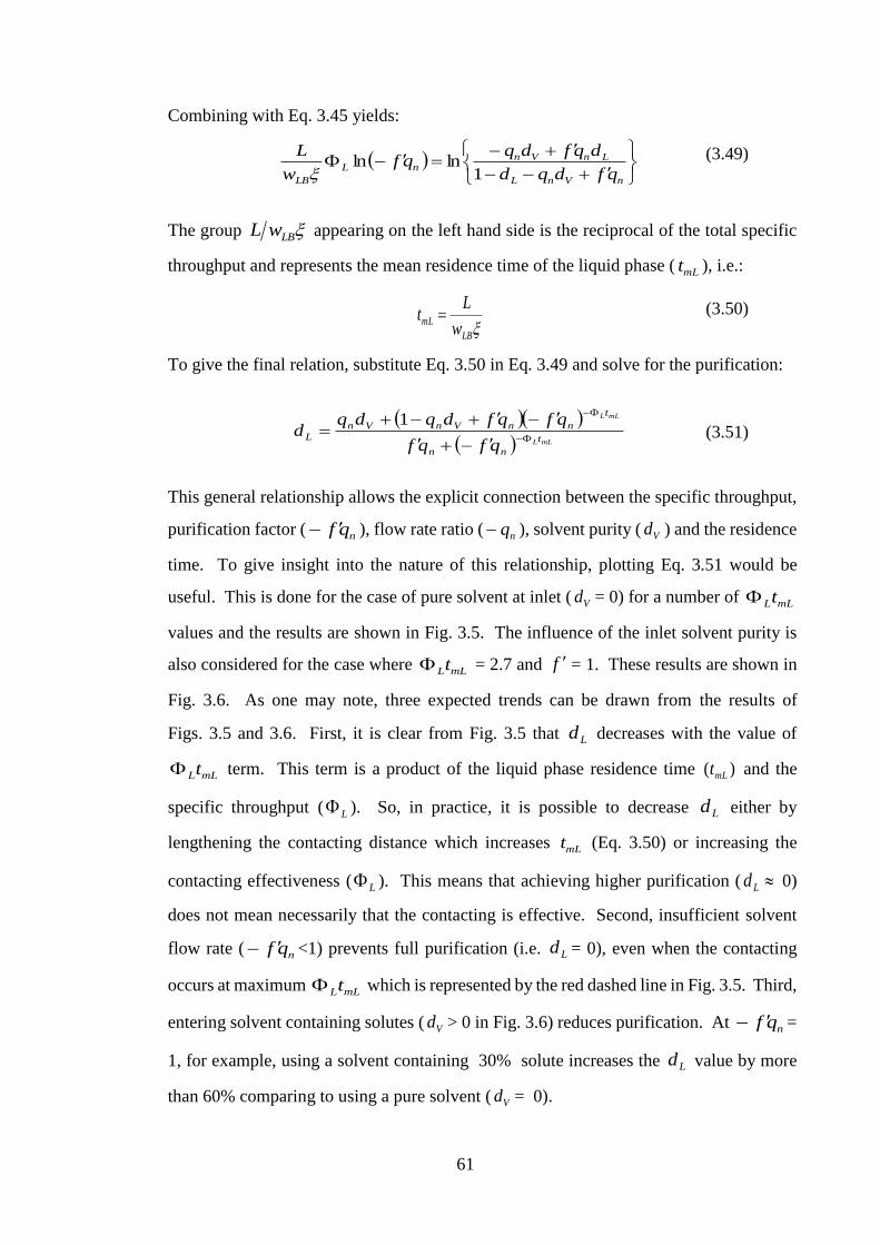
61
Combining with Eq. 3.45 yields:
( )
+−−
+−=−
nVnL
LnVnnL
LB qfdqd
dqfdqqf
w
L
1lnln
(3.49)
The group LBwL appearing on the left hand side is the reciprocal of the total specific
throughput and represents the mean residence time of the liquid phase ( mLt ), i.e.:
LB
mLw
Lt = (3.50)
To give the final relation, substitute Eq. 3.50 in Eq. 3.49 and solve for the purification:
( )( )
( ) mLL
mLL
t
nn
t
nnVnVnL
qfqf
qfqfdqdqd
−
−
−+
−+−+=
1 (3.51)
This general relationship allows the explicit connection between the specific throughput,
purification factor ( nqf − ), flow rate ratio ( nq− ), solvent purity ( ) and the residence
time. To give insight into the nature of this relationship, plotting Eq. 3.51 would be
useful. This is done for the case of pure solvent at inlet ( = 0) for a number of mLLt
values and the results are shown in Fig. 3.5. The influence of the inlet solvent purity is
also considered for the case where mLLt = 2.7 and = 1. These results are shown in
Fig. 3.6. As one may note, three expected trends can be drawn from the results of
Figs. 3.5 and 3.6. First, it is clear from Fig. 3.5 that decreases with the value of
mLLt term. This term is a product of the liquid phase residence time )( mLt and the
specific throughput ( L ). So, in practice, it is possible to decrease either by
lengthening the contacting distance which increases mLt (Eq. 3.50) or increasing the
contacting effectiveness ( L ). This means that achieving higher purification ( Ld 0)
does not mean necessarily that the contacting is effective. Second, insufficient solvent
flow rate ( nqf − <1) prevents full purification (i.e. = 0), even when the contacting
occurs at maximum mLLt which is represented by the red dashed line in Fig. 3.5. Third,
entering solvent containing solutes ( > 0 in Fig. 3.6) reduces purification. At nqf − =
1, for example, using a solvent containing 30% solute increases the value by more
than 60% comparing to using a pure solvent ( = 0).
Vd
Vd
f
Ld
Ld
Ld
Vd
Ld
Vd
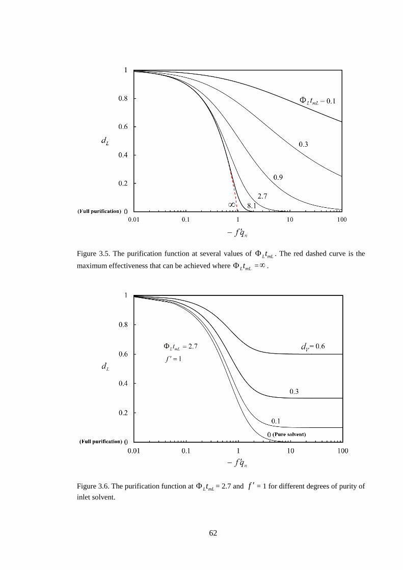
62
Figure 3.5. The purification function at several values of mLLt . The red dashed curve is the
maximum effectiveness that can be achieved where mLLt = .
Figure 3.6. The purification function at mLLt = 2.7 and = 1 for different degrees of purity of
inlet solvent.
f

63
3.6 Modification for Rotating Packed Beds
The relations developed so far can be applied to any counter-current contacting
device for which the body force is constant and hence the flow conditions remain uniform
along the contacting length. This situation holds to a good approximation for packed
columns, falling film columns and rotating spirals. However, relations for rotating
packed beds differ since the geometry is cylindrical with flow in the radial direction as
shown in Fig. 3.7. This means that the velocity and the section area vary radially along
the bed. So it should be expected that the volumetric mass transfer coefficient also varies
with the radial position and some adjustments are needed to the relations given in the
preceding sections.
Making a material balance on a solute being desorbed in a differential element has a
volume rHdr2 (Fig. 3.7), the relations corresponding to Eqs. 3.24 and 25 are:
( )
( )
−=−
O
I
OL
IL
r
r
L
L
rY
rY LBLB
LB rdraKN
H
YY
dY 2
)( (3.52)
( )
( )
=−
O
I
OV
IV
r
r
V
V
rY
rY VBVB
VB rdraKN
H
YY
dY 2
)( (3.53)
where is the bed void fraction and LN and VN are the phase molar flow rates which
can be expressed in terms of the area available for the flow (fA ) and velocity as
fLBLL AwnN = and ( ) fVBVV AwnN −= 1 .
Integration of the left hand side is exactly as before, but the right hand side varies in the
integration because the mass transfer coefficients and the interface area per unit volume
are functions of r . The usual treatment for rotating packed bed is to use average products
of the mass transfer coefficients and specific interface area (e.g. Chiang et al., 2009).
Accordingly, the mass transfer coefficient relations corresponding to Eqs. 3.32 and 3.33
are:
( ) ( ) ( )
LB
ILBOLB
L
IOL
Y
rYrY
N
rrHaK
−=
−−
22 (3.54)
( ) ( ) ( )
VB
IVBOVB
V
IOV
Y
rYrY
N
rrHaK
−=
− 22 (3.55)

64
H
dr
(a) (b)
rI
rO
z
Heavy
phase
Light
phase
rfb
H
The relation for a specific throughput is unchanged, although it is now in terms of the
average mass transfer coefficients. Thus, the equivalent of Eq. 3.43 becomes,
( )
( )nn
n
L
LL
qfqf
qf
n
aK
−
+=
ln
1 (3.56)
Similar to Eq. 3.45, Eq. 3.54 can be expressed in terms of the inlet and outlet mole fraction
ratios:
( )( )
+−−
+−=
+−
nVnL
LnVn
nL
nIOL
qfdqd
dqfdq
qfN
qfrrHaK
1ln
1 22
(3.57)
The relation for the number of stages (Eq. 3.46) and hence for the total specific throughput
(3.47) is unchanged. Further, from Eqs. 3.56 and 3.57, the same relation for purification
as before holds (Eqs. 3.51) with the mean residence time given by passage volume per
volumetric flow rate in this case.
( )
L
IOmL
Q
rrHt
22 −=
(3.58)
Figure 3.7. Rotating packed bed: (a) bed geometry where H is the axial height, Ir bed inner
radius and Or outer radius and (b) an element taken at radial position r .
65
3.7 Summary
Bulk mass transfer analysis for counter-current contacting was carried out in this
chapter. As a result, useful relations were derived and will be used along this study. The
first relations developed here were those for the overall mass transfer coefficients (Eqs.
3.32, 3.33, 3.54 and 3.55). These relations are used to estimate the overall transfer
coefficients from the experimental measurements (inlet and outlet bulk solute
compositions and the phase flow rates). Relations for the specific throughput (Eqs. 3.43)
and the total specific throughput (Eq. 3.47) were also developed here. These terms are
used to assess the spiral contacting effectiveness and to compare the spiral with other
alternative approaches. Finally, a novel design equation (Eq. 3.51) that links the mass
transfer parameters was presented in this chapter. This relation is used to help
interpretations, to check the consistency of the experimental data and to calculate
values from the computational results.
So far relations based on bulk quantities to analyse experiments under different
conditions have been presented. These relations can be applied to desorption process in
any fluid-fluid phase contactors. For absorption process, the relations are not quite
different and they are presented at the end of Chapter 7 to compare absorption and
desorption results. However, understanding the mass transfer process in a rotating spiral
channel needs a precise model that allows prediction and detailed analysis. Such model
is considered in this work and is presented in the next chapter.
Ld
66
Chapter Four
4 Modelling of Two-phase Contacting in a Rotating
Spiral Channel
A computational model is presented in this chapter. The model is employed in this
work to investigate the process of gas-liquid contacting in a rotating spiral channel. The
concept of this model is based on a 2-D numerical solution of the flow and species
equations using an interface shape computed independently using the interface model of
MacInnes and Zambri (2015). This allows prediction of the true character of the main
flow and Coriolis secondary motion. These parameters are of primary importance since
they determine the mass transfer mechanism in the channel and hence gain insight into
the details of rotating spiral contacting. Further, knowing the flow and species fields
allows the individual mass transfer coefficients to be quantified. These coefficients are
the most important parameters of interest since they determine the specific throughput
and hence the effectiveness of contacting.
The chapter is organised as follows: the governing equations and the appropriate
approximations for the spiral flow are given first. This is followed by a presentation of
the interface model and the required boundary conditions. After that, the numerical
solution is discussed and a series of computations is conducted. The purpose of these
computations is to understand the general behaviour of gas-liquid contacting and to
investigate the main effects of the gas and liquid phase flow rate that are tested
experimentally. The chapter closes with the analytical solution for an infinite-width
channel (MacInnes et al., 2012), which is used here to assess the 2-D numerical solution.
Model Description
The physical situation of two immiscible phases contacting in a rotation spiral
channel is depicted in Fig. 4.1 where a heavy and a light phase flow counter-currently
with a dilute solute transferring between them. The figure shows the coordinate system,
the channel geometry and a 2-D section through the channel along with the nomenclature
used.

67
a) Channel Segment b) 2-D section
Figure 4.1. Coordinate system and channel geometry: (a) segment of a spiral channel and (b) the
2-D section.
Since practical spiral channels have relatively a large radius of curvature in relation
to the channel height ( hR ), the channel is treated as straight at any location and is
inclined at angle relative to the tangential direction (Fig. 4.1 a). The validity of this
approximation has been verified by performing computations using local cylindrical
coordinates fit to a section of the spiral channel. In Fig. 4.1, x and y are coordinates of
the flow section and z is the direction along the channel. u , v and w represent the
velocity components in the x, y and z direction, respectively. The axis of rotation is
parallel to the x direction and the channel is located at a distance R from the channel wall
to this axis. The channel section (Fig. 4.1 b) has height h and width W . In the section,
the heavy phase occupies fraction of the flow area ( hW ) which is determined by the
position and shape of the phase interface. For the counter-current contacting of interest,
the heavy phase is driven primarily by the centrifugal effect and flows as a layer over the
outer wall in the positive z direction. For the light phase, which has much lower density,
the flow is driven mainly in the opposite direction by the pressure gradient.
As discussed in Chapter 2 (Section 2.4.4), MacInnes et al. (2012) argue that a stable
layer flow must be obtained when flow conditions are laminar and below critical values
of the Froude and Weber numbers (Eq. 2.17). Hence, flow in the spiral channel below
these critical conditions and for dilute solute concentration is considered laminar,
isothermal and steady in each phase.
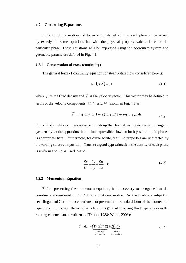
68
Centrifugal
acceleration
Coriolis
acceleration
Governing Equations
In the spiral, the motion and the mass transfer of solute in each phase are governed
by exactly the same equations but with the physical property values those for the
particular phase. These equations will be expressed using the coordinate system and
geometric parameters defined in Fig. 4.1.
4.2.1 Conservation of mass (continuity)
The general form of continuity equation for steady-state flow considered here is:
( ) 0= V
(4.1)
where is the fluid density and V
is the velocity vector. This vector may be defined in
terms of the velocity components ( u , v and w ) shown in Fig. 4.1 as:
kji )()(),,( zy,x,wzy,x,vzyxuV ++=
(4.2)
For typical conditions, pressure variation along the channel results in a minor change in
gas density so the approximation of incompressible flow for both gas and liquid phases
is appropriate here. Furthermore, for dilute solute, the fluid properties are unaffected by
the varying solute composition. Thus, to a good approximation, the density of each phase
is uniform and Eq. 4.1 reduces to:
0=
+
+
z
w
y
v
x
u
(4.3)
4.2.2 Momentum Equation
Before presenting the momentum equation, it is necessary to recognise that the
coordinate system used in Fig. 4.1 is in rotational motion. So the fluids are subject to
centrifugal and Coriolis accelerations, not present in the standard form of the momentum
equations. In this case, the actual acceleration ( a
) that a moving fluid experiences in the
rotating channel can be written as (Tritton, 1988; White, 2008):
VRaa ++= 2)(ref. (4.4)
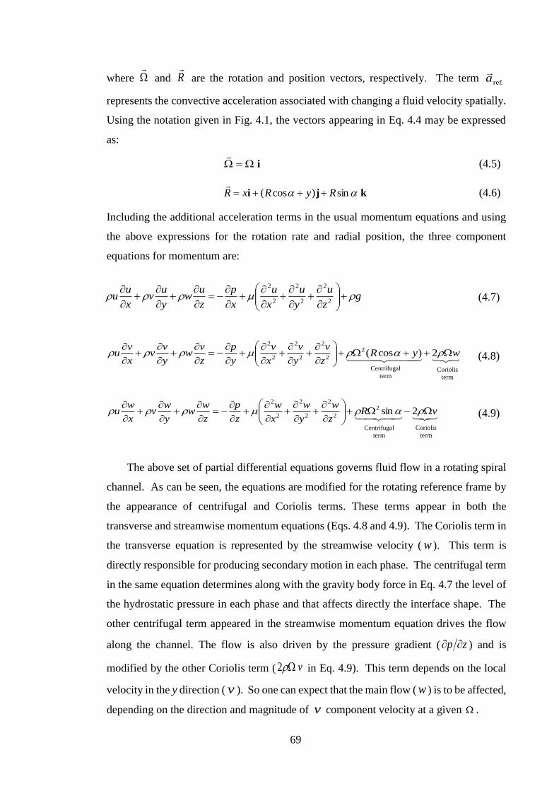
69
Coriolis
term
Coriolis
term
Centrifugal
term
Centrifugal
term
where
and R
are the rotation and position vectors, respectively. The term ref.a
represents the convective acceleration associated with changing a fluid velocity spatially.
Using the notation given in Fig. 4.1, the vectors appearing in Eq. 4.4 may be expressed
as:
i=
(4.5)
kji sin)cos( RyRxR +++=
(4.6)
Including the additional acceleration terms in the usual momentum equations and using
the above expressions for the rotation rate and radial position, the three component
equations for momentum are:
gz
u
y
u
x
u
x
p
z
uw
y
uv
x
uu +
+
+
+
−=
+
+
2
2
2
2
2
2
(4.7)
wyRz
v
y
v
x
v
y
p
z
vw
y
vv
x
vu +++
+
+
+
−=
+
+
2)cos(2
2
2
2
2
2
2
(4.8)
vR
z
w
y
w
x
w
z
p
z
ww
y
wv
x
wu −+
+
+
+
−=
+
+
2sin2
2
2
2
2
2
2
(4.9)
The above set of partial differential equations governs fluid flow in a rotating spiral
channel. As can be seen, the equations are modified for the rotating reference frame by
the appearance of centrifugal and Coriolis terms. These terms appear in both the
transverse and streamwise momentum equations (Eqs. 4.8 and 4.9). The Coriolis term in
the transverse equation is represented by the streamwise velocity ( w ). This term is
directly responsible for producing secondary motion in each phase. The centrifugal term
in the same equation determines along with the gravity body force in Eq. 4.7 the level of
the hydrostatic pressure in each phase and that affects directly the interface shape. The
other centrifugal term appeared in the streamwise momentum equation drives the flow
along the channel. The flow is also driven by the pressure gradient ( zp ) and is
modified by the other Coriolis term ( v2 in Eq. 4.9). This term depends on the local
velocity in the y direction ( v ). So one can expect that the main flow ( w ) is to be affected,
depending on the direction and magnitude of v component velocity at a given .

70
4.2.3 Species Conservation Equation
The transport of a solute in a rotating spiral channel could occur in x, y, and z
directions by two mechanisms: molecular diffusion and convection by fluid motion. The
general form of the solute conservation equation including these two terms in the absence
of chemical reaction is given as (Bird et al., 1997):
( ) ( )
YnDYVn 2= (4.10)
where n is the molar density, D the solute mass diffusivity and Y the solute mole
fraction. In terms of Cartesian coordinates, Eq. 4.10 can be expressed:
+
+
=
+
+
2
2
2
2
2
2
z
Y
y
Y
x
YD
z
Yw
y
Yv
x
Yu (4.11)
As can be seen, the three velocity components appear explicitly in Eq. 4.11, showing a
clear dependency of solute transport on Coriolis secondary motion and the streamwise
velocity.
Up to this point, the governing equations have been presented for laminar,
incompressible flow but are otherwise general. More approximations, however, are
appropriate in the case of the contacting flow in rotating spiral channels. These are
examined next.
4.2.4 Two-dimensional Approximations
The driving force remains constant along the channel, provided the component sinR
remains constant and the density and viscosity are uniform in each phase. The former is
ensured by the correct design of the spiral and corresponds to a spiral that maintains a
fixed spacing between revolutions (Chapter 2, Section 2.4.2). The latter follows from the
approximately constant composition in each phase. Hence, beyond an entry length at
either end of a spiral channel, the flow will be independent of the z direction for uniform
phase properties and no mass exchange between the phases, except a transfer of a dilute
solute. This developed flow state is two-dimensional with velocity components dependent
only on x and y direction and also the pressure gradient is constant along the channel and
independent of x and y. This is an excellent approximation in a channel of uniform
Diffusion term Convection term
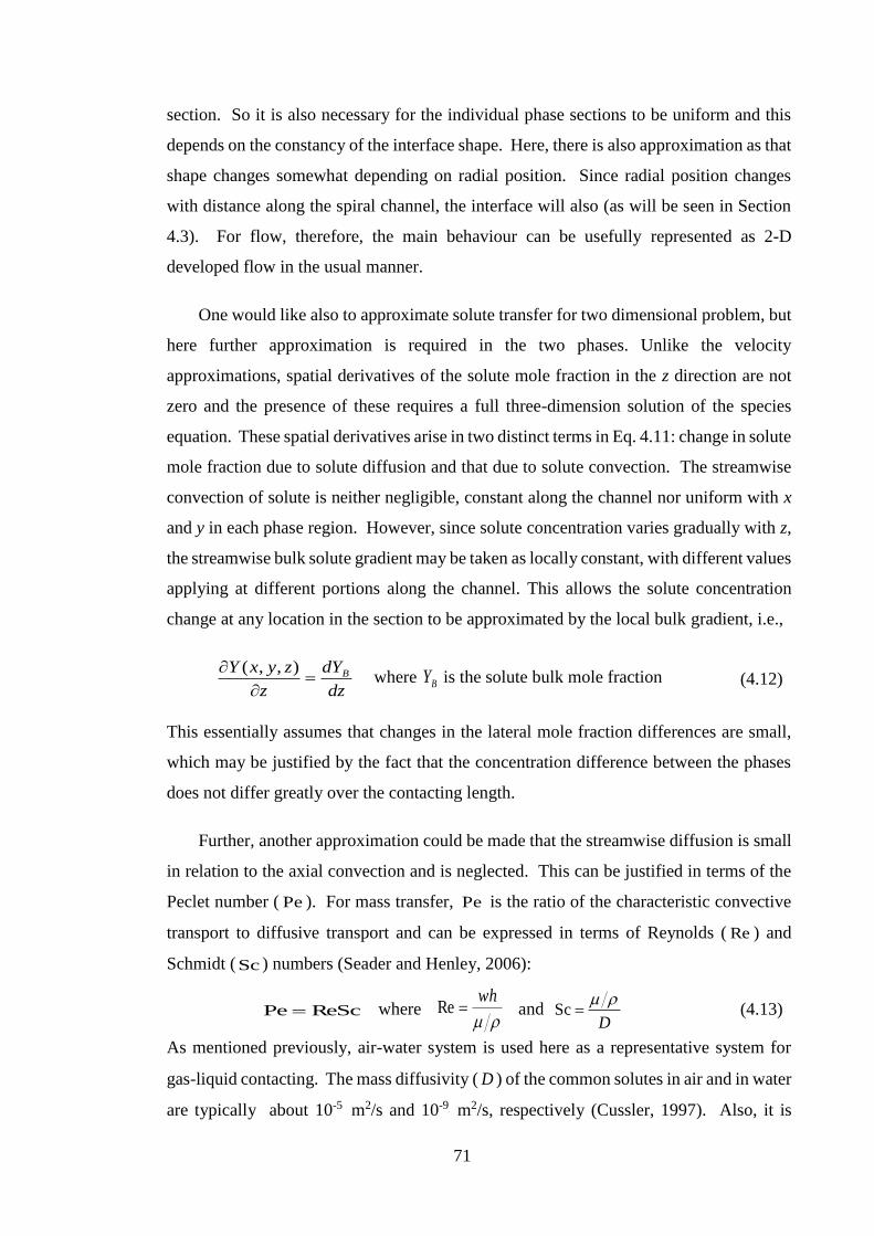
71
section. So it is also necessary for the individual phase sections to be uniform and this
depends on the constancy of the interface shape. Here, there is also approximation as that
shape changes somewhat depending on radial position. Since radial position changes
with distance along the spiral channel, the interface will also (as will be seen in Section
4.3). For flow, therefore, the main behaviour can be usefully represented as 2-D
developed flow in the usual manner.
One would like also to approximate solute transfer for two dimensional problem, but
here further approximation is required in the two phases. Unlike the velocity
approximations, spatial derivatives of the solute mole fraction in the z direction are not
zero and the presence of these requires a full three-dimension solution of the species
equation. These spatial derivatives arise in two distinct terms in Eq. 4.11: change in solute
mole fraction due to solute diffusion and that due to solute convection. The streamwise
convection of solute is neither negligible, constant along the channel nor uniform with x
and y in each phase region. However, since solute concentration varies gradually with z,
the streamwise bulk solute gradient may be taken as locally constant, with different values
applying at different portions along the channel. This allows the solute concentration
change at any location in the section to be approximated by the local bulk gradient, i.e.,
dz
dY
z
zyxY B=
),,( where BY is the solute bulk mole fraction (4.12)
This essentially assumes that changes in the lateral mole fraction differences are small,
which may be justified by the fact that the concentration difference between the phases
does not differ greatly over the contacting length.
Further, another approximation could be made that the streamwise diffusion is small
in relation to the axial convection and is neglected. This can be justified in terms of the
Peclet number ( Pe ). For mass transfer, Pe is the ratio of the characteristic convective
transport to diffusive transport and can be expressed in terms of Reynolds ( Re ) and
Schmidt (Sc ) numbers (Seader and Henley, 2006):
ReScPe = where
wh=Re and
D
=Sc (4.13)
As mentioned previously, air-water system is used here as a representative system for
gas-liquid contacting. The mass diffusivity ( D ) of the common solutes in air and in water
are typically about 10-5 m2/s and 10-9 m2/s, respectively (Cussler, 1997). Also, it is
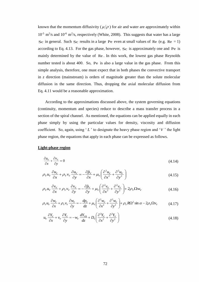
72
known that the momentum diffusivity ( ) for air and water are approximately within
10-5 m2/s and 10-6 m2/s, respectively (White, 2008). This suggests that water has a large
Sc in general. Such Sc results in a large Pe even at small values of Re (e.g. Re = 1)
according to Eq. 4.13. For the gas phase, however, Sc is approximately one and Pe is
mainly determined by the value of Re . In this work, the lowest gas phase Reynolds
number tested is about 400. So, Pe is also a large value in the gas phase. From this
simple analysis, therefore, one must expect that in both phases the convective transport
in z direction (mainstream) is orders of magnitude greater than the solute molecular
diffusion in the same direction. Thus, dropping the axial molecular diffusion from
Eq. 4.11 would be a reasonable approximation.
According to the approximations discussed above, the system governing equations
(continuity, momentum and species) reduce to describe a mass transfer process in a
section of the spiral channel. As mentioned, the equations can be applied equally in each
phase simply by using the particular values for density, viscosity and diffusion
coefficient. So, again, using ‘ L ’ to designate the heavy phase region and ‘V ’ the light
phase region, the equations that apply in each phase can be expressed as follows.
Light-phase region
0=
+
y
v
x
u VV (4.14)
+
+
−=
+
2
2
2
2ˆ
y
u
x
u
x
p
y
uv
x
uu VV
VVV
VVV
VV (4.15)
VV
VVV
VVVV
VVV w
y
v
x
v
y
p
y
vv
x
vu +
+
+
−=
+
2
ˆ2
2
2
2
(4.16)
VVV
VVV
0VVV
VVV vR
y
w
x
w
dz
dp
y
wv
x
wu −+
+
+−=
+
2sin2
2
2
2
2
(4.17)
+
+−=
+
2
2
2
2
y
Y
x
YD
dz
dYw
y
Yv
x
Yu VV
VVB
VV
VV
V (4.18)
73
Heavy-phase region
0=
+
y
v
x
u LL (4.19)
+
+
−=
+
2
2
2
2ˆ
y
u
x
u
x
p
y
uv
x
uu LL
LLL
LLL
LL (4.20)
LL
LLL
LLLL
LLL w
y
v
x
v
y
p
y
vv
x
vu +
+
+
−=
+
2
ˆ2
2
2
2
(4.21)
LLLLL
L0L
LLL
LL vRy
w
x
w
dz
dp
y
wv
x
wu −+
+
+−=
+
2sin2
2
2
2
2
(4.22)
+
+−=
+
2
2
2
2
y
Y
x
YD
dz
dYw
y
Yv
x
Yu LL
LLB
LL
LL
L (4.23)
It is important to note that the pressure appearing in the above equations ( Vp , Lp )
is a piezometeric pressure in the flow section. In most cases of flow in rotating or curved
channels, the true pressure can be expressed in a reduced form (piezometeric) in
x-y section. Usually, this is made by combining the gravity force in Eq. 4.7 and
the transverse centrifugal force in Eq. 4.8 with xp and yp , respectively
(e.g. Speziale and Thangam, 1983; Beak and Ko, 2000; Lee and Beak, 2002). In general,
such treatment is acceptable since the effect of gravity and transverse centrifugal force
are present whether there is flow or not and balance the pressure gradient in x and y
directions in both cases. So these forces do not have any influence on the main flow and
can be combined with the pressure force terms. Accordingly, the actual pressure
derivatives in the transverse directions (Eqs. 4.7 and 4.8) and the centrifugal and gravity
terms in the same equations may reduce to:
In Eq. 4.7: gx
p
x
p−
=
ˆ (4.24)
In Eq. 4.8: 2)cos(
ˆ+−
=
yR
y
p
y
p (4.25)
where p is the piezometeric pressure and can be found at any point in x-y section by
integrating Eqs. 4.24 and 4.25, thus for the light phase and heavy phase:
74
),()2
cos(),(),(ˆ0
22
yxpgxy
Ryyxpyxp VVVV −
++−= (4.26)
),()2
cos(),(),(ˆ0
22
yxpgxy
Ryyxpyxp LLLL −
++−= (4.27)
In the above equations, 0Vp and 0Lp are reference pressures taken at the position x = 0
and y = 0 on the phase interface (Fig. 4.1).
Finally, the bulk mole fraction gradients in the light and heavy phase ( dzdYLB and
dzdYVB ) appearing in Eqs. 4.18 and 4.23 are related through solute conservation and
thus are not independent. Equating mass transfer rates in the two phases at the interface
and using Eqs. 3.1 and 3.2 (given in Chapter 3) requires that:
dz
dYwn
dz
dYwn VB
VBVLB
LBL )1( −=− (4.28)
Hence, setting the bulk gradient in one phase determines that in the other.
Interface Shape
The part of the channel section occupied by each phase must be established to solve
the governing equations. Two parameters determine these sections: the interface shape
and its location inside the channel. These two parameters depend on fluid flow and can
be obtained simultaneously as part of the solution of the flow equations (Wörner, 2012).
MacInnes and Zambri (2015), however, point out that for practical conditions in the spiral
the component of centrifugal acceleration driving the flows is far smaller than the
transverse component that determines interface shape, i.e. sincos 22 RR ,
since is small. This means that the interface shape is insignificantly affected by flow
stresses and can be calculated independently of the flow solution, considering only the
effect of stresses at static conditions and surface tension. The pressure difference across
the interface (stresses), the interfacial surface tension, , and the interface shape are
linked by Young-Laplace law as:
+=−
21
11
rrpp LV (4.29)

75
where 1r and 2r are respectively the curvature radii of the interface in the x-y section and
along the channel. For rotating spiral contacting, the difference in pressure across the
interface )( LV pp − can be determined directly from Eqs. 4.26 and 4.27 by setting
LV pp ˆˆ = . Therefore, according to the coordinates given in Fig. 4.2, LV pp − can be
written as:
−+−+=− gxy
yRppp VLLV
2
0 )2
cos()( (4.30)
where 000 LV ppp −= at x = 0 and y = 0 (Fig. 4.1 or Fig. 4.2 below).
Eq. 4.29 can be simplified by dropping 21 r since the curvature of the interface along the
channel is smaller than that in the transverse direction, 11 r . Further, since hR and
1cos for small , the term 2cos yR + in Eq. 4.30 can be approximately replaced
by the outer wall radial position ( 0R in Fig. 4.2). Using these simplifications and taking
rr =1 , substitution of Eq. 4.30 into Eq. 4.29 results in:
=−−+
rgxyRp VL
1))(( 2
00 (4.31)
Figure 4.2. An illustrative diagram showing the geometry of the interface in a section of spiral
channel. 1W and 2W are the contact angles at both ends.
The radius ( r ) in Eq. 4.31 can be expressed in terms of the arc length ( ) to obtain
parametric equations for the interface coordinates. Normalising by the channel width, the
resulting equations can be written as (MacInnes and Zambri, 2015):

76
*
***
2
*
02*
*2
d
dxxy
Wp
d
yd
C
−
+=
(4.32)
2/12
*
*
*
*
1
−=
d
dy
d
dx (4.33)
The asterisked indicates normalised variables: Wyy =* , Wxx =* , W =* and
*
0
* pWp = . In addition, two new parameters emerge from this non-dimensional
representation: the characteristic capillary height ( WC ) and the gravity parameter ( ):
22
0)( WRW VL
C
−=
and 2
0=
R
g (4.34)
WC is the root of the ratio of the interfacial surface force to the centrifugal force. This
parameter reflects the relative characteristics meniscus height for the interface. Thus, the
smaller the value of WC the more effective the centrifugal force is to overcome the
interface curvature and hence results in a flatter interface between the two phases. On the
other hand, indicates to what degree the interface is tilted due to the effect of gravity
(Eq. 4.34). In general, as the rotation rate increases, the effect of gravity becomes minor
and approximately less tilted interface can be obtained at a given radial position.
From Eqs. 4.32, 4.33 and 4.34, it is clear that the shape of the interface depends only
on the phase density difference ( VL − ), surface tension ( ), the radial position of the
interface along the spiral ( 0R ), the channel width (W ) and the rotation rate ( ). Also,
the shape depends on the contact angles ( 1W and 2W in Fig. 4.2) which determine the
slope at the end-walls:
**
**
1
11
cos
sintan
ddy
ddx
W
WW
−==
,
**
**
2
22
cos
sintan
ddy
ddx
W
WW ==
(4.35)
Specifying these parameters, the profile of the interface can be determined by numerical
integration of Eqs. 4.32 and 4.33 over a given channel width. The solution starts from
both ends where the slopes are defined by the contact angles (Eq. 4.35). The solution also
requires adjustment of *
0p in Eq. 4.32 at either side such that the arc length extends
from each end to match (having the same slope) at a central point (MacInnes and Zambri,
2015).
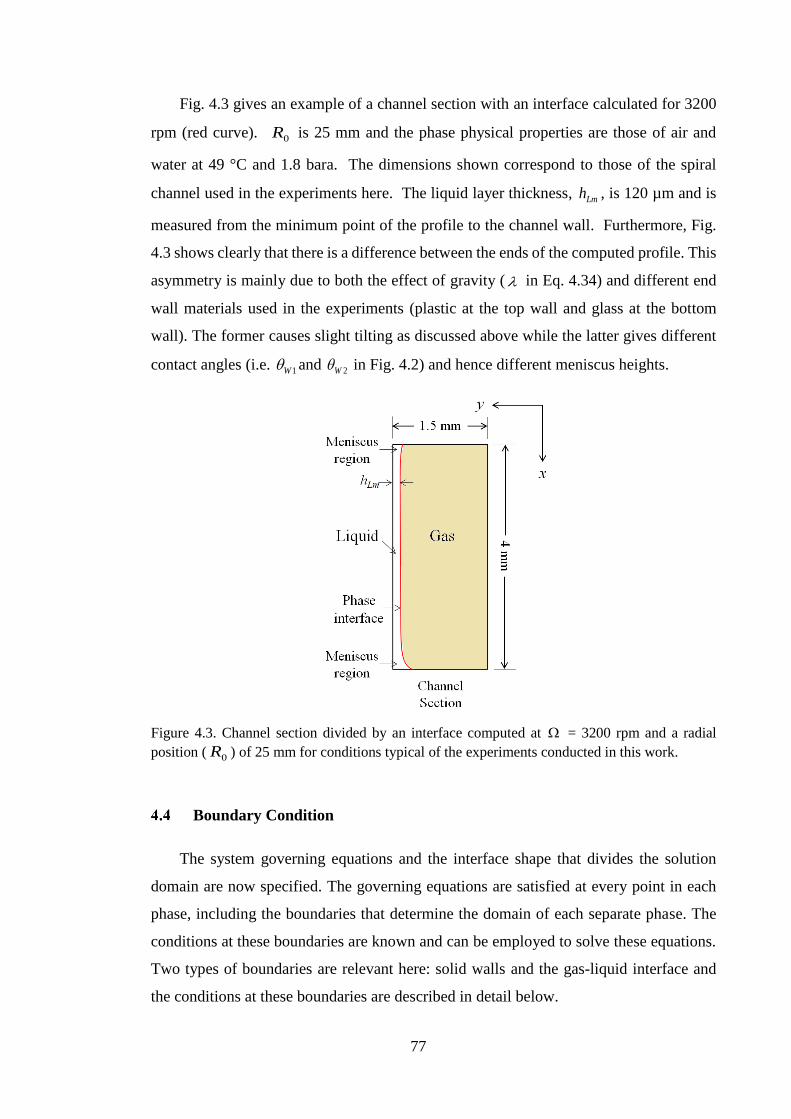
77
Fig. 4.3 gives an example of a channel section with an interface calculated for 3200
rpm (red curve). 0R is 25 mm and the phase physical properties are those of air and
water at 49 °C and 1.8 bara. The dimensions shown correspond to those of the spiral
channel used in the experiments here. The liquid layer thickness, Lmh , is 120 µm and is
measured from the minimum point of the profile to the channel wall. Furthermore, Fig.
4.3 shows clearly that there is a difference between the ends of the computed profile. This
asymmetry is mainly due to both the effect of gravity ( in Eq. 4.34) and different end
wall materials used in the experiments (plastic at the top wall and glass at the bottom
wall). The former causes slight tilting as discussed above while the latter gives different
contact angles (i.e. 1W and 2W in Fig. 4.2) and hence different meniscus heights.
Figure 4.3. Channel section divided by an interface computed at = 3200 rpm and a radial
position ( 0R ) of 25 mm for conditions typical of the experiments conducted in this work.
Boundary Condition
The system governing equations and the interface shape that divides the solution
domain are now specified. The governing equations are satisfied at every point in each
phase, including the boundaries that determine the domain of each separate phase. The
conditions at these boundaries are known and can be employed to solve these equations.
Two types of boundaries are relevant here: solid walls and the gas-liquid interface and
the conditions at these boundaries are described in detail below.

78
4.4.1 Walls
For fixed and non-absorbing walls, the conditions are no-slip velocity and zero
normal mass flux of solute. The mass flux can be expressed using the species flux vector
and the unit vector normal to the wall (i.e. ji yx nnn +=
). Using these expressions, the
boundary conditions at the wall surfaces in the light phase are:
Vu = 0 , Vv = 0 , Vw = 0 and 0=
+
y
VX
V ny
Yn
x
Y (4.36)
Similarly, where the heavy phase is in contact with the wall,
Lu = 0 , Lv = 0 , Lw = 0 and 0=
+
y
LX
L ny
Yn
x
Y (4.37)
4.4.2 Interface
The conditions at the interface can be obtained from the fact that the interface has a
negligible mass and therefore can store no momentum or mass. This constrains the
velocities to be continuous and the stress and mass flux to balance across the interface.
Further, since the macroscopic length scales are larger than the molecular spacing in both
the gas and the liquid, it is a good approximation that a local equilibrium prevails at the
interface. Additionally, the interface is fixed in the geometry section. This means that the
interface is not in motion in x-y plane and the normal velocity of the phases on the
interface is zero.
Now, in terms of the unit normal vector ( n
) to the interface, the conditions of the
velocity components at the interface are:
0=+ yVxV nvnu (normal velocity), 0=+ yLxL nvnu , LV vv = VL ww =, (4.38)
The stress at the interface has normal and tangential components. All components must
be balanced at each location on the interface. In the normal direction (Batchelor, 2000),
( ) ( ) ( ) ( ) ( ) ( ) yxVxyyVyyxVxxVyxLxyyLyyxLxxL nnnnpnnnnp 2ˆ2ˆ 2222 +++−=+++−
which, on substitution the Newtonian stress law gives:

79
yxVV
VyV
xV
VV
yxLL
LyL
xL
LL
nnx
v
y
un
y
vn
x
up
nnx
v
y
un
y
vn
x
up
+
+
+
+−
=
+
+
+
+−
22ˆ
22ˆ
22
22
(4.39)
)
It is important to note that the above equation is written in terms of the piezometeric
pressure ( Vp and Lp ), the same variable appearing in the flow equations. Expressing
Eq. 4.39 in this way means that the surface tension effect is implicitly taken into account.
This is clear from the expression of the piezometeric pressure (Eqs. 4.26 and 4.27) which
includes the effect of hydrostatic pressure that balances r (Eq. 4.31). Thus, it must be
expected that at static conditions, Eq. 4.39 can reduce to the scalar Young-Lapace
equation given in Eq. 4.29, as expected.
It is also important to emphasise here that the normal stress will not be balanced
precisely since the interface shape is calculated for conditions where the flow stresses
make no contribution to the pressure change across the interface. Excluding the flow
stresses from Eq. 4.39 means that at all positions on the interface, the piezometeric
pressure should remain the same on either side, as assumed in the interface model. This
constraint is imposed on the interface at the wall contact line which corresponds to the
point (0,0) in Fig. 4.1. In this case, differences in piezometeric pressure across the
interface in the 2-D computation reflect the extent to which flow stresses affect interface
shape and hence the error in interface shape determination. A typical pressure deviation
at 3200 rpm, for example, is about 20 Pa. This corresponds to less than 1% of the
centrifugal pressure difference taken into account in the interface shape.
The balance of the tangential stress components in the x-y plane results in (Batchelor,
2000),
( ) ( ) ( ) ( ) ( ) ( )2222
yxVxyyxVyyxxyxLxyyxLyyxx nnnnnnnn −+−=−+−
or
( )
( )22
22
2
2
yxVV
VyxVV
V
yxLL
LyxLL
L
nnx
v
y
unn
x
u
y
v
nnx
v
y
unn
x
u
y
v
−
+
+
−
=−
+
+
−
(4.40)
80
There is other tangential stress component in the z direction. This is expressed
( ) ( ) ( ) ( ) yVyzxVxzyLyzxLxz nnnn +=+
so,
The solute flux must also be balanced at the interface. This requires:
Finally, the solute mole fraction jump across the interface is expressed:
where VIY and LIY are the values of solute mole fraction along the interface in the light
and heavy phase, respectively.
Numerical Solution
A direct solution for the 2-D governing equations given in Section 4.2.4 is not
possible even with the simplification made. The equations are nonlinear and coupled
through the conditions at the interface and hence a numerical solution is required.
Comsol Multiphysics Software (general PDE mode) can be used to achieve the numerical
solution. The applicability and accuracy of this software to handle different partial
differential equations (PDEs) have been demonstrated in many entries to the literature
(e.g. Zimmerman, 2004; Li et al., 2009). In Comsol, the numerical solution is based on
the finite element method (FEM) in which the computational domain is discretised into
small subdomains, forming a mesh of cells (Fig. 4.4). The generated mesh determines
locations (nodes) over the solution domain. At these nodes, the variables are calculated
by approximating the PDEs to a set of algebraic equations and solving them. Typically,
a large number of nodes is used to obtain a reliable solution. In turn, this leads to a large
number of algebraic equations which are solved often by iteration to reach a converged
solution.
Before describing the computational method used to solve the governing equations,
there are three essential parameters should be selected to achieve an accurate numerical
yV
VxV
VyL
LxL
L ny
wn
x
wn
y
wn
x
w
+
=
+
(4.41)
yV
VVxV
VVyL
LLxL
LL ny
YDnn
x
YDnn
y
YDnn
x
YDn
+
=
+
(4.42)
)( LIVI YfY = (4.43)

81
Linear Quadratic Cubic
Nodes
Domain
Boundary
solution. These parameters are the shape, type and size of the elements. In this work, the
basic and the most commonly used parameters are selected and this will be discussed
first.
Figure 4.4. An arbitrary domain discretised using triangular elements.
4.5.1 Shape of Element
Triangular elements are often preferred in representing irregular domain shape since
they involve less error compared to other 2-D element shapes (Reddy, 1984; Ho-Le, 1988;
Pepper and Heinrich, 2006). The irregularity, in this case, arises from the curving shape
of the interface as shown in Fig. 4.3. So triangular elements are used throughout this
work to generate the mesh in each separate domain.
4.5.2 Type of Element
As a default choice, Comsol Multiphysics uses Lagrange polynomials as the
interpolation function to describe the variation of variables within the elements. Elements
are classified according to the order of the interpolation polynomial (linear, quadratic,
cubic, etc.). The difference between these types is just the number of nodes used for the
Lagrange function to represent a variable over an element (the higher polynomial order
the more nodes are needed and hence higher order element). Fig. 4.5 shows the number
of nodes in triangular elements up to third order.
Figure 4.5. Types of triangular elements up to cubic order.

82
The common approach to obtaining a stable numerical solution for the
incompressible Navier-Stokes equation is to use mixed element types where the pressure
should be less than the velocity by one order. Typically, quadratic Lagrange element for
the velocity components and linear Lagrange element for the pressure are employed
(Reddy, 1984; Zimmerman, 2004; Olesen et al., 2006; Gregersen et al., 2009; Sheng and
Zhu, 2014). Such treatment is because that the order of velocity in the momentum
equations is higher than that for pressure. Hence, for consistency, the order of the
Lagrange function used for the pressure should be less than that used for the velocities
(Reddy, 1984). Here, first-order and second-order Lagrange elements are used for the
pressure and the velocity component, respectively. For the solute mole fraction, second-
order elements are also used since they give accurate results with a reasonable
computation time when a suitable element size is selected.
4.5.3 Element Size Distribution
The size of elements determines the accuracy of the solution. The smaller the
element size, the better the approximation and hence the more accurate solution can be
achieved. But this accuracy is at the expense of increased computational time and
memory. To reduce that, elements with different sizes in a non-uniform mesh are used
and distributed so that size suits accuracy requirement in each location.
At the molar flow rate ratio of interest, the contacting occurs in the spiral between a
thin liquid layer (small ) and a gas phase occupied most the channel (typically as that
shown in Fig. 4.3). This is mainly due to the inherent difference between the molar
densities of the contacting phases which results in a smaller liquid volumetric flow rate
relative to that for the gas phase. Thus, one should expect a small mesh size is needed in
the liquid side to compute accurately the velocity and concentration fields in such small
spatial scale. Further, the liquid phase in general, as argued previously, has a larger
Schmidt number comparing to the gas phase which is typically around one. So one should
expect also a much steeper concentration gradient in the liquid side since larger Sc
results in larger Peclet number even at small values of Reynolds number (i.e. )1ReL ,
according to Eq. 4.13. This also suggests that a small element size is needed in the liquid
side. Another location required to be treated carefully is the region around the interface.
This region is strongly curved at the end-walls. Furthermore, since the mass flux and the
stresses must match at the interface, an abrupt change in the velocity and concentration

83
field occurs there due to the difference in the properties of the contacting phases.
Consequently, a small size of elements needs to be placed near the interface compared to
the element size in the far field.
Considering the regions where small element size is expected to be needed, a finer
grid size by a factor of 8 to10 times is used in the liquid domain as compared to that in
the gas. Further, the maximum element growth rate, which determines the maximum
allowable size ratio of two adjacent elements, is constrained in both regions to be 1.1.
This ensures a large number of small elements to be packed in the region around the phase
interface. So the curved boundary between the two phases and the large change in the
solution gradients there can be captured reliably. The other element size parameters
which can be adjusted are the curvature factor (which is the ratio of element size to the
curved boundary radius) and the minimum allowable element size. These are left as
specified in Comsol to be 0.2 and 8 10-5 mm, respectively, since they are sufficiently
small to obtain a mesh independent solution as will be described subsequently.
As an illustrative example, Fig. 4.6 below shows the elements distribution using the
size parameters discussed above. The maximum element size in the gas and liquid
side used are 0.3 mm and 0.03 mm, respectively, giving a total number of elements, NE,
of 5259.
Figure 4.6. Non-unifrom mesh using maximum element size of 0.3 mm and 0.03 mm in the gas
and liquid side, respectively.

84
4.5.4 Quantities Derived from the Numerical Solution
The solution of the governing equations gives the velocity, pressure and
concentration values at any x and y coordinates in the spiral section. As a result, the bulk
flow rate and concentration, and the mass transfer coefficient in each phase can be
determined. These bulk quantities are of interest since they can be measured
experimentally and hence a numerical analysis and comparison with the experiments are
possible.
Since both phases have a uniform density along the channel, the bulk flow rates can
be determined directly by integrating the streamwise velocity ( Vw and Lw ):
V
A
VVVBV dAwAwQ
V
== and L
A
LLLBL dAwAwQ
L
== (4.44)
where VBw and LBw are the bulk velocities and VA and LA are the section areas occupied
by the light and heavy phase, respectively.
Similarly, the bulk mole fraction in each phase ( VBY and LBY ) can be found by dividing
the integration of the product of velocity and mole fraction by the volumetric flow rate:
V
A
VV
VVB
VB dAYwAw
Y
V
=1
and =
LA
LLL
LLB
LB dAYwAw
Y1
(4.45)
In terms of the individual mass transfer coefficients ( Vk and Lk ), they can be calculated
locally from the fact that the mass transfer rate in each phase must equal the total amount
of solute transferred across the interface. Taking the interface length as I in the channel
section, this balance may be expressed in an appropriate form as:
Light phase: dz
dYAwndYnDnYYk VB
VVBVIVVVVBVIIV
I
==−
)( (4.46)
Heavy phase: dz
dYAwndYnDnYYk LB
LLBLILLLLILBIL
I
−==−
)( (4.47)
where the bulk solute mole fraction ( BY ) are calculated from Eqs. 4.45 and VIY and LIY
can be found by integrating VY and LY along the interface length ( I ):

85
dYY
I
V
I
VI =1
and
dYY
I
L
I
LI =1
(4.48)
It is helpful to indicate here that for rotating spiral contacting, the interfacial area per unit
volume of the passage ( a ) can be calculated easily since the geometry of the space
occupied by each phase is known:
A
a I= (4.49)
where A is the cross-section area of the channel ( hW ).
Thus, when values of volumetric mass transfer coefficients are required, it is just a matter
of multiplying the values of Vk and Lk calculated from Eqs. 4.46 and 4.47, respectively,
by the value of a from Eq. 4.49.
It should be clear now that having obtained a full solution, the bulk flow rate
( VQ and LQ ) and bulk mole fraction in each phase ( VBY and LBY ) can be calculated from
Eq. 4.44 and 4.45, respectively. VIY and LIY can be calculated from Eq. 4.48. These
results then allow determination of the individual mass transfer coefficients ( Vk and Lk )
using Eqs. 4.46 and 4.47. From these coefficients, the overall mass transfer coefficient
based on one of the phases can be found using the relations given in Chapter 3 (Eq. 3.26).
The degree of purification ( ) can also be determined using the purification formula
(Eq. 3.51).
4.5.5 Solution Approach
A number of input parameters are required to solve the governing equations (Eqs.
4.14 to 4.23) using the boundary conditions given in Section 4.4. These parameters are
the pressure gradient ( dzdp0 ), the bulk solute mole fraction gradient ( dzdYB ) in each
phase, the rotation rate ( ), the liquid layer thickness along with the physical properties
of each phase and the geometric parameters ( sinR ). The properties of the phases
( , and D ) and the solute equilibrium distribution ( ) can easily be determined at a
given spiral temperature and pressure. This is discussed in details in Chapter 6. The
geometric parameters of the spiral are fixed and the rotation rate can be decided. Using
this information, the shape of the interface can be computed at any radial position along
Ld
f

86
the channel by solving the equations of the interface model (as described in Section 4.3).
Once the interface shape has been determined, the interface position can be decided,
determining the liquid layer thickness ( Lmh ) and hence the flow domain for each phase as
shown in Fig. 4.3. In the numerical solution, the liquid phase flow rate is sensitive to the
liquid layer thickness while the gas phase flow rate is determined mainly by the level of
dzdp0 set. In terms of species equation, dzdYLB and dzdYVB are linked by the solute
conservation constraint (Eq. 4.28), so value of just a single bulk mole fraction gradient is
required. Furthermore, since only gradients of pressure and mole fraction appear in the
equations, it is necessary to specify the level of each at some position in the section to
close the solution.
To predict what happens in the experiments, it is necessary to compute the volumetric
flow rates at which the contacting occurs. Numerically, obtaining a solution (i.e. velocity
and mole fraction distribution) directly for a given gas and liquid flow rate is not possible.
This requires adjusting, by trial and error, both the value of the pressure gradient and the
liquid layer thickness to compute particular phase flow rates. In this work, however, it
will be often of interest to solve for a given gas phase flow rate and compute a number of
different liquid phase flow rates. Thus, for a given liquid layer thickness, it is only
necessary to adjust the pressure gradient along the channel to match the gas phase flow
rate with the liquid flow rate determined from the solution. For the solute, as pointed out,
setting one of the bulk mole fraction gradient ( dzdYLB or dzdYVB ) and a reference
solute mole fraction determines (together with the flow solution) the mole fraction field
in both phases ( VY and LY ). The bulk mole fraction gradient is selected such that avoids
the value of mole fraction distribution falling outside the physically-possible range which
is between zero to unity at all positions in the section.
As mentioned previously, the general PDE mode in Comsol Multiphysics (Ver.5.2)
is employed to achieve the numerical solution. In this mode, the governing equations for
both phases and the relevant boundary conditions are implemented using a general PDE
equation. Details concerning the implementation of the governing equations and the
boundary conditions in Comsol are described in Appendix A. The equations are solved
using an iterative solver with a relative convergence tolerance of 10-6 which means that
the solution is converged only when the estimated error in the iterative calculation is less
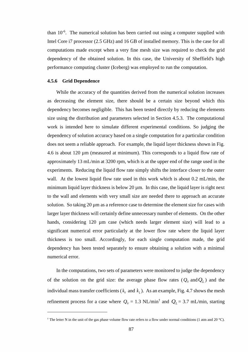
87
than 10-6. The numerical solution has been carried out using a computer supplied with
Intel Core i7 processor (2.5 GHz) and 16 GB of installed memory. This is the case for all
computations made except when a very fine mesh size was required to check the grid
dependency of the obtained solution. In this case, the University of Sheffield's high
performance computing cluster (Iceberg) was employed to run the computation.
4.5.6 Grid Dependence
While the accuracy of the quantities derived from the numerical solution increases
as decreasing the element size, there should be a certain size beyond which this
dependency becomes negligible. This has been tested directly by reducing the elements
size using the distribution and parameters selected in Section 4.5.3. The computational
work is intended here to simulate different experimental conditions. So judging the
dependency of solution accuracy based on a single computation for a particular condition
does not seem a reliable approach. For example, the liquid layer thickness shown in Fig.
4.6 is about 120 µm (measured at minimum). This corresponds to a liquid flow rate of
approximately 13 mL/min at 3200 rpm, which is at the upper end of the range used in the
experiments. Reducing the liquid flow rate simply shifts the interface closer to the outer
wall. At the lowest liquid flow rate used in this work which is about 0.2 mL/min, the
minimum liquid layer thickness is below 20 µm. In this case, the liquid layer is right next
to the wall and elements with very small size are needed there to approach an accurate
solution. So taking 20 µm as a reference case to determine the element size for cases with
larger layer thickness will certainly define unnecessary number of elements. On the other
hands, considering 120 µm case (which needs larger element size) will lead to a
significant numerical error particularly at the lower flow rate where the liquid layer
thickness is too small. Accordingly, for each single computation made, the grid
dependency has been tested separately to ensure obtaining a solution with a minimal
numerical error.
In the computations, two sets of parameters were monitored to judge the dependency
of the solution on the grid size: the average phase flow rates ( VQ and LQ ) and the
individual mass transfer coefficients ( Vk and Lk ). As an example, Fig. 4.7 shows the mesh
refinement process for a case where VQ = 1.3 NL/min† and LQ = 3.7 mL/min, starting
† The letter N in the unit of the gas phase volume flow rate refers to a flow under normal conditions (1 atm and 20 °C).

88
from an initial grid of 8451 elements (NE). The specifications of each grid are
summarized in Table 4.1. The values of flow rates and mass transfer coefficients against
the number of elements are plotted in Figs. 4.8 and 4.9, respectively. It is clear from Fig.
4.8 that the effect of the mesh elements size on the phase flow rates is negligible beyond
NE > 8451 elements, leaving only slight differences which may be due to round-off errors.
The same behaviour can be seen for Vk in Fig. 4.9 but with an obvious change in Lk
values between 8451 < NE < 39,212. Thus, in this case, using NE 39,212 will ensure
that the sensitivity of VQ , LQ , Vk and Lk to the element size is negligible, giving a
maximum error less than 0.7% in Lk value when it is compared to that determined using
NE = 168,408.
It should be expected that using the same element size parameters listed in Table 4.1
for a lower liquid flow rate results in a larger error. Indeed, at LQ = 0.5 mL/min for the
same gas phase flow rate using the same parameters at NE = 39,212 (Table 4.1) leads to
an error about of 8% in Lk value in relation to that computed using the parameters at
NE =168,408. So a finer mesh is needed particularly in the liquid side to reduce the error
associated with decreasing the liquid flow rate and vice versa.
Figure 4.7. Different grids produced by Comsol using the element size parameters listed in Table
4.1.
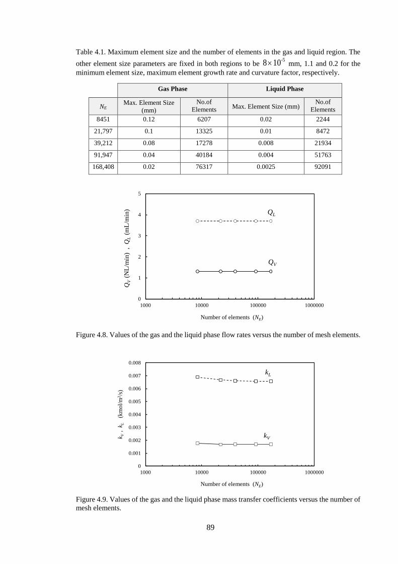
89
0
1
2
3
4
5
1000 10000 100000 1000000
QV
(N
L/m
in)
,
QL
(m
L/m
in)
Number of elements (NE)
QV
QL
0
0.001
0.002
0.003
0.004
0.005
0.006
0.007
0.008
1000 10000 100000 1000000
k V ,
kL
(
km
ol/
m2/s
)
Number of elements (NE)
kL
kV
Table 4.1. Maximum element size and the number of elements in the gas and liquid region. The
other element size parameters are fixed in both regions to be -5108 mm, 1.1 and 0.2 for the
minimum element size, maximum element growth rate and curvature factor, respectively.
Gas Phase Liquid Phase
NE Max. Element Size
(mm)
No.of
Elements Max. Element Size (mm)
No.of
Elements
8451 0.12 6207 0.02 2244
21,797 0.1 13325 0.01 8472
39,212 0.08 17278 0.008 21934
91,947 0.04 40184 0.004 51763
168,408 0.02 76317 0.0025 92091
Figure 4.8. Values of the gas and the liquid phase flow rates versus the number of mesh elements.
Figure 4.9. Values of the gas and the liquid phase mass transfer coefficients versus the number of
mesh elements.

90
Illustrative Computations
In this section, computations are carried out following the numerical solution
developed in the previous section. The objective of these computations is to investigate
the essential characteristics of rotating spiral contacting and the main effects of the gas
and liquid flow rate. The computations are made at =3200 rpm, which is used
experimentally, for a hypothetical solute desorbing from water into air at atmospheric
pressure and 20 °C. The phase properties at these conditions are listed in Table 4.2. The
values listed for the end-wall contact angles ( 1W and 2W ) are those established for the
experimental channel used here (MacInnes and Zambri, 2015) for the same phase system.
The geometry used in the computations also is for the experimental channel ( h and W as
those shown in Fig. 4.3 and sinR = 5.57 10-4 m).
Table 4.2. Properties of air-water system at 20 °C and 1 atm.
Phase
Properties Air Water
(kg/m3) 1.2 1000
(Pa s) 1.8 10-5 10-3
Solute
D (m2/s) 2 10-5 10-9
1
Interfacial properties
(N/m) 0.07
1W (glass) 15°
2W (plastic) 75°
4.6.1 General Behaviour
For rotation rate 3200 rpm, liquid layer thickness ( Lmh ) 50 µm and pressure gradient
( dzdp0 ) 2250 Pa/m, the computation produces counter-current flow with rates 3.5
NL/min and 2.5 mL/min for the gas phase and liquid phase, respectively. This
corresponds to − nqf 1 and so represents an appropriate condition of operation for the
particular solute value. Fig. 4.10 shows vector and contour plots of the computed
streamwise velocity, secondary motion and solute mole fraction fields.
f
f

91
x
y
Streamwise
velocitySecondary
motion
Solute
mole fraction
Domain
geometry
GasLiquid
In each phase, the colours are shaded from blue through green to red corresponding
to the range of values from minimum to maximum. In the liquid phase, the minimum w
velocity is at the channel walls and reaches a maximum near the interface. For the
counter-flowing gas flow, the velocity is generally negative and the minimum (dark blue)
occurs in the core of the flow away from the channel walls and interface where the
magnitude is greatest but velocity is negative. The velocity of the gas phase is thus
highest (red) at the walls and interface, where the liquid actually drags the gas in the
positive z direction. As pointed out previously, the interface shape is asymmetric both
since the end-wall contact angles differ (Table 4.2) and because gravity tilts the interface
slightly. The effect of the interface asymmetry on the streamwise liquid flow is quite
strong with considerably higher velocity in the lower thicker end of the layer (i.e. the dark
red core near the bottom end wall).
Figure 4.10. Numerical results for VQ = 3.5 NL/min and LQ = 2.5 mL/min at 3200 rpm:
streamwise velocity contours, vector plot revealing the secondary motion (arrow length
proportional to magnitude for each phase) and solute mole fraction contours.
The vector plot of the secondary motion reveals the primary effect of the Coriolis
acceleration. Without the term w2 in the y-component momentum equation (Eqs. 4.16
and 4.21) there would be no motion in either x or y. As discussed in Chapter 2 (Section
2.4.3), the secondary motion is produced by the non-uniformity of w velocity in x and y
directions. Fluid near the end walls has lower w velocity magnitude than that further

92
away so the pressure gradient that developed in the channel section overbalanced the slow
fluid near the walls but underbalanced that in the core region. The consequence is the
secondary motion near the end walls, which is magnified in the liquid phase, rotating in
the opposite direction in the two phases since they have opposite streamwise motion. It
can be noted that while the secondary motion affects the entire width of the flow in the
gas phase, it only penetrates into the liquid from the end walls at a distance approximately
similar to the liquid layer thickness.
Further, in Fig. 4.10, the effect of this secondary motion on the streamwise velocities
is clear in the distortion of gas streamwise velocity. Fig. 4.11 shows w velocity profile
along the y direction at mid-channel both with and without the Coriolis acceleration term
w2 that causes the secondary motion. To show clearly the velocity profile, w velocity
in each phase is normalised by its absolute maximum value, ranging the values of the
velocities from -1 to 1. So the difference (jump) between the velocities in Fig. 4.11 is
simply due to using different normalisation for the gas and liquid. As can be seen in Fig.
4.11, a strong asymmetric in the velocity profile (red line) is evident, confirming the
distortional effect of the Coriolis term in the streamwise momentum equation particularly
in the gas phase ( v− 2 ). Since is positive in this computation, this term serves to
drive the gas flow when Vv is positive and retard the gas flow when negative. Without
the term w2 , the numerical solution would, in turn, result in standard developed flow
profile for w (dashed line in Fig. 4.11), even including the Coriolis term v− 2 in the z-
component momentum equation. The streamwise velocity profile at the vertical centreline
of the gas layer is also plotted and shown in Fig. 4.12. While the profile is nearly
symmetric, it is also distorted by the strong Coriolis secondary motions at the top and the
bottom of the channel. This velocity profile shown in Fig. 4.12 is consistent with the
experimental observations of Hart (1971) for a single phase flowing in a channel at the
highest rotation rate tested (shown in Chapter 2, Fig. 2.15 e). Also, the distorted gas phase
velocity profile observed in Fig. 4.11 is qualitatively similar to the computed profiles
reported by Speziale (1982), Kheshgi and Scriven, (1985) and Beak and Ko (2000) which
are also for a single phase in a rectangular channel under rotation. This is, perhaps, not
surprising since the gas phase in the spiral occupied most the channel with a small fraction
of the liquid phase. So the flow in the spiral is approximately corresponding to a single
phase flow and hence a good agreement with the single phase literature results.

93
-1.2
-0.8
-0.4
0.0
0 0.5 1 1.5 2 2.5 3 3.5 4
W (mm)
Ω = 3200 rpm
Full terms
No Coriolis term
( )
max
/V
Vw
w
w2
W
-1.2
-0.8
-0.4
0.0
0.4
0.8
1.2
0 0.3 0.6 0.9 1.2 1.5
h (mm)
Ω = 3200 rpm
Liq
uid
-lay
er t
hic
kn
ess
Full terms
No Coriolis term
( )
max
max
/,
/L
LV
Vw
ww
w
max/ VV ww
max/ LL ww
w2
h
Figure 4.11. Normalised profile of the phase streamwise velocity at the centreline along the
y-axis in the absence and presence of Coriolis terms in the flow equations.
Figure 4.12. Normalised profile of the gas phase streamwise velocity at the vertical centreline in
the absence and presence of Coriolis terms in the flow equations.

94
x
y
Streamwise
velocity
Secondary
motion
Solute
mole fraction
The final contour plot of species distribution in the two phases reveals considerable
complexity. First of all, one notes extreme values appear in the core region of the gas
flow (solute minima). These are simply the results of strong convection of solute from
upstream in this high-speed core region, bringing gas of low solute concentration. The
top and bottom difference in streamwise velocity in the liquid associated with liquid layer
thickness variation appears to have a strong influence on solute distribution. Where liquid
velocity is low (top), gas and liquid may come to equilibrium and mass transfer is not
strong. Below, where streamwise liquid velocities are higher, variations in solute mole
fraction are more pronounced in the liquid and this has an evident effect on the gas
distribution.
4.6.2 Rotation Direction
The rotation direction may be positive or negative. The centrifugal terms are
insensitive to the rotation direction since they depend on the square of rotation value. The
Coriolis components, on the other hand, change sign and hence the direction of action.
This is examined here by repeating the computation in the previous computation but for
3200−= and compare the results. The same interface shape shown in Fig. 4.10 has
been used since the rotation direction does not change the level of the centrifugal force.
Also, the same phase flow rates in the previous computation have been re-produced here
by adjusting both the liquid layer thickness and the pressure gradient. Fig. 4.13 shows
the results at 3200−= rpm which are the same set of plots shown in Fig. 4.10.
Figure 4.13. Same set of plots shown in Fig. 4.10 but at −= 3200 rpm.

95
As in the previous computation, the gas phase streamwise velocity profile is distorted
but with high speed core region (blue) shifted towards the interface. This is consistent
with the expected flow reversal occurred in the secondary motion which is captured
correctly by the 2-D numerical solution. These changes in the flow pattern yield a
different mole fraction distribution in Fig. 4.13 than that shown in Fig. 4.10, particularly
in the gas side. In this case, lower solute mole fraction prevails in the most region of the
gas layer near the interface. As discussed previously, this is a result of the larger
streamwise velocity there, producing stronger convection of solute from upstream and
hence gas of lower solute mole fraction. In the liquid side, the streamwise velocity and
hence solute mole fraction distribution is not much sensitive to rotation direction. Thus,
similar to what has been observed in Fig. 4.10, the streamwise liquid velocity is high near
the bottom end wall (red core in the meniscus region) and it is low at the top, causing
variations in solute mole fraction along the layer. However, this variation is less
pronounced than that observed in Fig. 4.10.
Quantitatively, reversing the rotation rate leads to 10% increase in the liquid layer
thickness and approximately the same pressure gradient to re-produce the same phase
flow rates in the previous computation (values given in Table 4.3). In both computations,
the component sin2
0 +− Rdzdp L in the w equation is approximately the
same. So the increase in the liquid layer thickness is simply because the longitudinal
Coriolis term ( LL v− 2 ) is larger here than for positive case. Thus, one must
expect that this term lessens the component that drives the liquid phase when is
negative, leading clearly to such difference in the liquid layer thickness for the same liquid
phase flow rate. For the gas phase, on the other hand, VV v− 2 has a negligible effect
in Vw equation since the gas density is small. So changing the rotation direction does
not affect the pressure gradient and hence same value approximately has been obtained
(Table 4.3). In terms of the mass transfer coefficient, there is a slight reduction in aKL
value comparing with the previous computation and that is consistent with the increase
in the liquid layer thickness.

96
Table 4.3. Values of the liquid layer thickness, pressure gradient and overall volumetric mass
transfer coefficient for = 3200 and − 3200 rpm.
Quantities + −
Liquid layer thickness (µm) 50 55
dzdp0 (Pa/m) 2250 2270
aKL (kmol/m3/s) 1.07 0.98
4.6.3 Different Liquid Flow Rates
In this section, the variation of the liquid phase flow rate is examined. Fig. 4.14
shows the results of two different liquid flow rates where the rotation rate and the gas
phase are fixed as those used in the first computation ( = 3200 rpm and VQ = 3.5
NL/min). First of all, it is clear from the figure that the liquid layer thickness increases
with the liquid phase flow rate. The interface shape, as argued, is independent of the
phase flow rates. So the change in the interface position in Fig. 4.14 is only due to the
effect of the liquid flow rate. As mentioned in the previous section, the flow of the liquid
phase is mainly driven by the component 2sin RL (Eq. 4.22) along the channel
against the wall and gas phase shear stresses and the pressure force. This body force is
constant in both cases shown in Fig. 4.14 since the rotation rate is constant. So increasing
the liquid flow rate must produce a thicker layer to maintain balancing forces and hence
accommodate the increase in flow rate. Comparing with the images shown in Fig. 2.20 b
(MacInnes and Zambri, 2015), the same behaviour has been observed. That is, the liquid
layer thickness increases with the liquid phase flow rate at constant rotation rate.
It is also quite clear in Fig. 4.14 that the interface shape has a less effect on the
streamwise liquid flow as the liquid layer thickness increases. The liquid flow rate is
distributed approximately evenly with a higher velocity shifted towards the centre of the
layer (dark red core). Another point to note in Fig. 4.14 is that the secondary motion in
the liquid side evolves as the liquid flow rate increases. This is mainly due to increasing
the effect of the transverse Coriolis term ( LLw2 ) in the Lv equation. As can be seen in
the vector plot, the configuration of this motion in the liquid phase starts with two
vortices, occupying the menisci regions at small LQ . As increasing LQ then, the
structure of the secondary motion develops by producing small streamwise vortices (roll
cells), stretching gradually towards the middle of the liquid layer. The effect of these roll
cells is quite evident in the solute mole fraction contour plot.

97
x
y
Liquid Gas
Streamwise
velocity
Secondary
motion
Solute
mole fraction
Domain
geometry
Liquid Gas
Figure 4.14. Numerical results at LQ = 1.2 mL/min and LQ = 12 mL/min. The rotation rate is
3200 rpm and VQ = 3.5 NL/min.
In terms of the mass transfer quantities, Fig. 4.15 shows the values of the mass
transfer coefficients. As can be seen, a noticeable increase in the individual liquid phase
transfer coefficient (grey bar) as the liquid phase flow rate increases. This could be
attributed to the developed secondary flow in the liquid side which can boost the mass
transfer rate, resulting in a larger mass transfer coefficient. Fig. 4.16 provides information
about the solute molar flux along the interface for the two different LQ cases. As can be
seen, the mass transfer rate is improved as the liquid flow rate increases, as expected. The
peaks in the plot (black curve) correspond to locations where the streamwise vortices are
active, indicating clearly the role of secondary motion in enhancing the mass transfer.
(a) QL = 1.2 mL/min
(b) QL = 12 mL/min
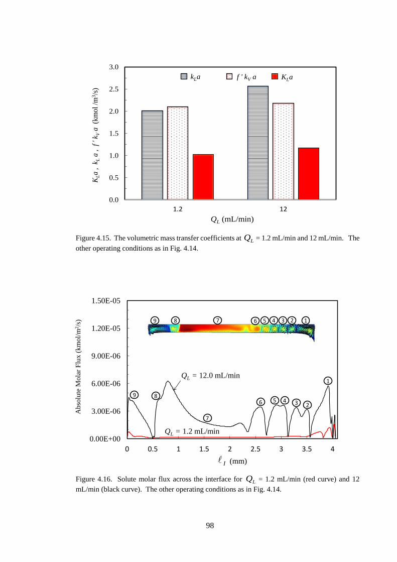
98
0.00E+00
3.00E-06
6.00E-06
9.00E-06
1.20E-05
1.50E-05
0 0.5 1 1.5 2 2.5 3 3.5 4
Abso
lute
Mola
r F
lux (
km
ol/
m2/s
)
(mm)
5
7
4 17 23
1
34569
9
I
8
8
2
6
QL = 12.0 mL/min
QL = 1.2 mL/min
0.0
0.5
1.0
1.5
2.0
2.5
3.0
1.2 12
Series1 Series2 Series3
QL (mL/min)
KLa , k L
a ,
f ' k
Va (k
mol
/m3/s
)
KLa kLa f ' kV a
Figure 4.15. The volumetric mass transfer coefficients at LQ = 1.2 mL/min and 12 mL/min. The
other operating conditions as in Fig. 4.14.
Figure 4.16. Solute molar flux across the interface for LQ = 1.2 mL/min (red curve) and 12
mL/min (black curve). The other operating conditions as in Fig. 4.14.

99
4.6.4 Different Gas Flow Rates
The variation of the gas phase flow rate is now examined by computing for a range
from 1 to 6 NL/min with the liquid phase flow rate held constant at LQ = 2.5 mL/min.
This range of gas phase flow rate gives a range of Reynolds numbers approximately
between 300 and 1800. So it falls within the laminar flow regime where the 2-D model
equations can be applied. The computed streamwise velocity, secondary flow and solute
mole fraction distribution for the highest and lowest gas phase flow rate are shown in Fig.
4.17 and will be discussed first.
As can be seen in the figure, the general features observed in the previous
computations do not change as the gas phase flow rate changes however there are some
interesting points that can be made. First, comparing to the effect of liquid phase flow
rate, it is quite clear that the gas phase has a minor effect on the liquid layer thickness.
The computations show that increasing the gas phase flow rate by a factor of 6 requires
adjusting the liquid layer thickness ( Lmh ) by about 20% (from 45 to 55 µm) to maintain
the same liquid phase flow rate. This behaviour is linked directly to the layer thickness
which is quite thin at 3200 rpm. At such thin layer, the order of magnitude of shear stress
exerted by the gas on the liquid phase interface is small in relation to the wall shear stress
(MacInnes and Zambri, 2015). Hence, the liquid layer thickness is slightly sensitive to
the variation of gas phase flow rate at this particular rotation rate, which is considered
relatively high. However, as the rotation rate decreases, Lmh increases and the effect of
gas phase flow rate may become more pronounced. This is simply because the thicker
layer provides a smaller flow passage available for the gas phase. This leads, in turn, to
increasing the gas shear stress on the liquid side due to both increasing the gas velocity
and decreasing the characteristic spatial length. This is tested here by re-producing the
conditions of Fig. 4.17 but for = 1480 rpm. At this rotation rate, Lmh = 110 µm and
dzdp0 = 600 Pa/m produce counter-current flow with VQ = 1 NL/min and LQ = 2.5
mL/min. Increasing Lmh and dzdp0 to be 356 µm and 6000 Pa/m, respectively, counter-
current flow with VQ = 6 NL/min and LQ = 2.5 mL/min can be produced. So, clearly,
the results show that under the same variation of gas phase flow rate (from 1 to 6 NL/min),
the liquid layer thickness increases by approximately 3 times (from 110 to 356 µm) at the
low rotation rate. These computational results are consistent with the experimental

100
Streamwise
velocity
Secondary
motion
Solute
mole fraction
Domain
geometry
Liquid Gas
x
y
Liquid Gas
observations of MacInnes and Zambri (2015) shown in Chapter 2. The images at
= 1480 rpm (Fig. 2.20 d) show the strong sensitivity of the liquid layer thickness to the
gas phase flow rate while this sensitivity becomes negligible at =3840 rpm over
approximately the same range of gas phase flow (Fig. 2.20 c).
Figure 4.17. Numerical results at = 3200 rpm and LQ = 2.5 NL/min for two different gas phase
flow rates.
Another effect of gas phase flow rate observed in Fig. 4.17 is on Coriolis secondary
motion. The velocity vectors for the two cases are plotted using the same scale factor,
showing clearly that the strength of secondary motion in the gas side increases as the
(a) NL/min0.1=VQ
(b) NL/min0.6=VQ

101
0.0
0.5
1.0
1.5
2.0
2.5
0 1 2 3 4 5 6 7
QV (NL/min)
KLa
, k L
a ,
f ' k V
a (k
mol
/m3/s
)
KLa
kL a
f ' kV a
gas flow rate increases. This is mainly due to the effect of the term VV w2 which
determines the strength of this motion. The consequence of increasing the secondary
motion on the main flow is also evident in Fig. 4.17, relatively thinner momentum layers
at the two end walls at the higher gas phase flow rate
Bringing in mind the observations discussed above, the mass transfer mechanism can
be understood. Fig. 4.18 shows the variation of the mass transfer coefficients over the
computed range of gas phase flow rate. It is obvious that the individual gas phase mass
transfer coefficient increases with the gas phase flow rate. This is consistent with the
noticeable improvement in Coriolis secondary motion with the gas phase flow rate. This
convective motion, in effect, can short-circuit the species diffusion and hence enhances
mass transfer. On the other side, the individual liquid phase mass transfer coefficient
decreases slightly with the gas phase flow rate. This is clearly attributed to the slight
increase in the liquid layer thickness which decreases the species diffusion. Based on the
behaviour of these individual parameters, the overall mass transfer coefficient increases
slightly with the gas phase flow rate, showing a clear dependency on the mass transfer
action in both phases.
Figure 4.18. Values of the individual and overall mass transfer coeffiecnets over the computed
range of gas phase flow rate where = 3200 rpm and LQ = 2.5 NL/min.
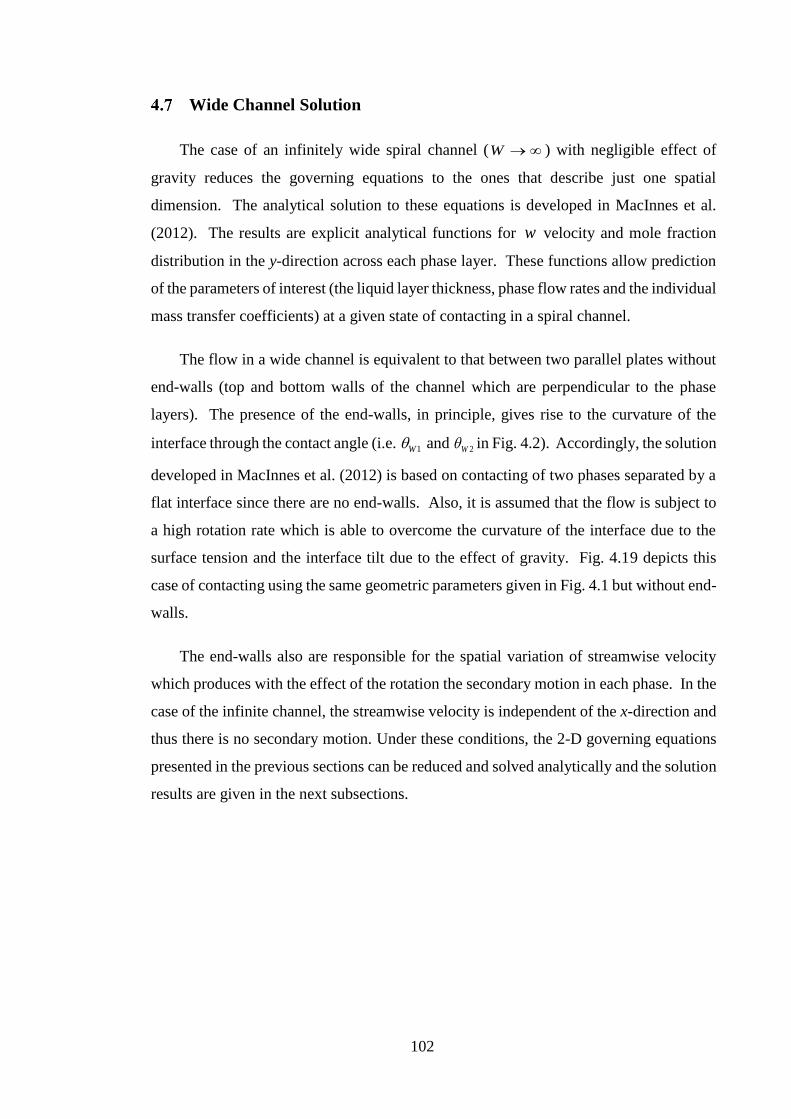
102
Wide Channel Solution
The case of an infinitely wide spiral channel ( →W ) with negligible effect of
gravity reduces the governing equations to the ones that describe just one spatial
dimension. The analytical solution to these equations is developed in MacInnes et al.
(2012). The results are explicit analytical functions for w velocity and mole fraction
distribution in the y-direction across each phase layer. These functions allow prediction
of the parameters of interest (the liquid layer thickness, phase flow rates and the individual
mass transfer coefficients) at a given state of contacting in a spiral channel.
The flow in a wide channel is equivalent to that between two parallel plates without
end-walls (top and bottom walls of the channel which are perpendicular to the phase
layers). The presence of the end-walls, in principle, gives rise to the curvature of the
interface through the contact angle (i.e. 1W and 2W in Fig. 4.2). Accordingly, the solution
developed in MacInnes et al. (2012) is based on contacting of two phases separated by a
flat interface since there are no end-walls. Also, it is assumed that the flow is subject to
a high rotation rate which is able to overcome the curvature of the interface due to the
surface tension and the interface tilt due to the effect of gravity. Fig. 4.19 depicts this
case of contacting using the same geometric parameters given in Fig. 4.1 but without end-
walls.
The end-walls also are responsible for the spatial variation of streamwise velocity
which produces with the effect of the rotation the secondary motion in each phase. In the
case of the infinite channel, the streamwise velocity is independent of the x-direction and
thus there is no secondary motion. Under these conditions, the 2-D governing equations
presented in the previous sections can be reduced and solved analytically and the solution
results are given in the next subsections.

103
Figure 4.19. Two phase contacting in a wide spiral channel: (a) a segment of a spiral channel
without end-walls and (b) top view showing the geometric parameters.
4.7.1 Hydrodynamic Parameters
The relevant parts of the solution of the flow equations are the phase volumetric
flow rates ( VQ and LQ ). Here, these values are measured experimentally and hence a
direct comparison with the experiments can be made by reproducing these measured
values. The full analytical expressions for VQ and LQ are given in MacInnes et al. (2012)
and can be re-expressed as:

104
r
)1(1
)41)(1)(1()1(3)1(
12
2
0
3
r
rrrrr
V
Vdz
dpWhQ
−−
+−−−+−−−= (4.50)
)1(1
))1(4()1()1)(1(3
12
22
0
3
r
rrrrr
V
Ldz
dpWhQ
−−
+−−+−−−= (4.51)
where r and r are ratios of viscosity and density for the two phases,
L
Vr
= and
L
Vr
= (4.52)
and r is the ratio of centrifugal body force acting on the heavy phase to the pressure
force:
2
0
sin=
dzdp
RLr
(4.53)
Eq. 4.53 can be expressed in terms of flow rate ratio ( LV QQq = ) and phase physical
properties by dividing Eq. 4.50 by Eq. 4.51 and solving for r :
(4.54)
The above equations allow the essential hydrodynamic parameters of two phase
contacting in a rotating spiral channel to be predicted. For example, from Eqs. 4.50 to
4.54, the liquid layer thickness represented by can be predicted at given phase
flow rates by knowing only the phase physical properties ( r and r ), the geometric
parameters ( ,W h and the component sinR ) and the rotation rate. From , q and
the phase physical properties, r can be calculated from Eq. 4.54. Then, the pressure
gradient along the channel can be found straightforward from Eq. 4.53.

105
4.7.2 Mass Transfer Coefficients
In terms of the mass transfer parameters, it is sufficient to introduce the expressions
for the individual mass transfer coefficient since these are the most relevant parameters
and allow a comparison with the experiments through the overall mass transfer coefficient
of one of the phases. These expressions are given in MacInnes et al. (2012) as:
2
2
2
)())(1())(1(213
41)(1(3)4(2135
FEDCBAh
Dnk
rr
rrrrrVVV
+++−++−+
+−−+−−−−−=
(4.55)
2
2
2
)()(2
))944()1(33)1(235
KJIHGDnh
Dnk
rrrr
rrrrVVL
++−+
−−+−+−−−+=
(4.56)
The normalised physical properties used in Eqs. 4.55 and 4.56 are the same for those in
r but with two additional parameters: ratios of molar density ( rn ) and solute diffusion
coefficient ( rD ) and these are:
L
Vr
n
nn = and
L
Vr
D
DD = (4.57)
Further, r and can be calculated independently, as mentioned, from the hydrodynamic
equations while the variables A to K are functions only of the physical properties and
and can be found from the equations listed in Table 4.4 (MacInnes et al, 2012).
Some characteristics can be drawn from the infinite-width channel solution. First,
the mass transfer coefficients are independent of the solute mole fraction gradient along
the channel ( dzdYLB and dzdYVB ) and nor do they depend on the level of the solute
mole fraction. Second, at a constant phase flow rates ratio (which is determined by the
solute equilibrium distribution, ) and constant interface position ( ), Vk and Lk are
independent of the level of the flow rate in each phase.
f

106
Table 4.4. Functions used in Eqs. 4.55 and 4.56.
4)1(41387 2 −−−−= rrrA
13)4113)(1())3334(439(8239)1( 2 −−−+−−−−−= rrrrrrB
rrrrC 13)1(4)1(1463 242 +−−+=
rrrD 66)1(41(2)2(1313)1( 22 +−+−+−=
)1341()1(2 3 −−= rE
)5(10(10513)8213(132)1( 2 −−−−−−+−= rF
22)1(13)1(3056367063 rrrG −−−−−+−=
9))1(45()1(7 2 −−+−= rrH
2)1341)(1()269(2814191 rrrrI −−−+−−−=
rrrJ 4)1(13)1(14)1(63 242 +−−+−=
)13)1(82()2(1321322 rrK +−+−+=
Comparison with Wide-channel Solution
The wide-channel case can be employed to assess the 2-D numerical solution by
comparing the predictions of these two different approaches to solve the governing
equations. To reduce the 2-D numerical model to the wide-channel case, the interface
shape is treated as flat and symmetry boundary conditions are applied at the end-walls of
the spiral channel. The symmetry condition imposes zero normal velocity and vanishing
both viscous stresses and solute diffusion flux at the end walls. In this way, the effect of
the end-walls is neglected and the problem is approximated to two-phase contacting in a
channel with large aspect ratio ( →hW ). The comparison has been done over different
phase flow rate ratios (0.2 nq 12) using the same phase physical properties (Table
4.2), rotation rate and channel geometry used in the previous computations.
As expected, the same analytical results of the wide channel solution have been re-
produced numerically over the whole range of the conditions tested. Fig. 4.20 shows
representative results of a computation made at LQ = 8.198 mL/min, VQ = 3 NL/min and
= 3200 rpm using symmetry boundary conditions at the end walls. On the left is the

107
x
y
Streamwise
velocity
Solute
mole fraction
Domain
geometry
GasLiquid
domain geometry where a flat interface divides the gas and the liquid phase. The variation
of the velocity field and the flow direction of the phases can be seen from streamwise
velocity contour plot. Qualitatively, the dark blue core in the gas region is the highest
velocity (negative value) while the highest liquid phase velocity is approximately at the
interface (red) and is a positive value. So, clearly, the phase streamwise velocities change
only in the lateral y-direction and counter-current mode of flow is achieved. On the right
is the solute mole fraction distribution in each phase and also, clearly, it varies only in the
y-direction. By choosing a negative solute mole fraction gradient in the liquid phase,
desorption mode of contacting is depicted here where the solute is being transferred from
the liquid phase into the gas phase. The values of the individual mass transfer coefficients
computed by the two solution approaches at the conditions shown in Fig. 4.20 are listed
in Table 4.5.
Figure 4.20. Numerical results for LQ = 8.198 mL/min and VQ = 3 NL/min at 3200 rpm, using
a flat interface and applying symmetry boundary conditions at the end-walls.
Table 4.5. Values of the volumetric mass transfer coefficient calculated from the wide channel
analytical solution (MacInnes et al. 2012) and the 2-D numerical solution.
Solution Approach akV
(kmol /m3/s)
akL
(kmol /m3/s)
Analytical Solution (Eqs. 4.55 and 4.56 ) 1.0686 1.2230
Numerical Solution (Eqs. 4.46 and 4.47) 1.0673 1.2230

108
Summary
This chapter introduced a 2-D numerical model to simulate a mass transfer process
of a dilute solute between two phases contacting in a section of rotating spiral channel.
In the chapter, the main aspects of the numerical solution were described and illustrative
computations were carried out. These computations served to highlight the general
behaviour of counter-current gas-liquid contacting in a rotating spiral channel and the
effects of gas and liquid phase flow rate individually. Hydrodynamics results of these
computations were compared qualitatively with the previous experimental measurements
and theoretical predictions for a single phase in a channel under rotation and the results
were in agreement. At the end of this chapter, the analytical solution for a case where the
spiral channel has infinite width was presented (MacInnes, et al, 2012) and a direct
comparison with the 2-D numerical solution at symmetry boundary conditions was
carried out.
The main conclusions from the computations made for the experimental channel,
which has a relatively large aspect ratio, can be summarised as follows:
• As a general behaviour, strong Coriolis secondary motion in the gas phase
occupied most of the channel while there are just two weak vortices in the
liquid phase and they reside mainly in the meniscus regions.
• The streamwise velocities are distorted due to the effect of Coriolis
acceleration.
• At fixed rotation rate ( =3200 rpm), increasing the gas phase flow rate
produces stronger Coriolis motion. This motion improves the mass transfer
in the gas side with a small effect on the liquid layer thickness.
• In the liquid phase, on the other hand, increasing the liquid phase flow
increases the liquid layer thickness and changes the structure of Coriolis
secondary motion. The motion becomes strongly active in the corners and
generates small vortices, stretching gradually towards the central layer. This
developed motion also can enhance mass transfer in the liquid side by
convection.

109
Chapter Five
5 Mass Transfer Experiments
This chapter describes the experiments conducted in this thesis. The objective of
these experiments is to investigate the performance of rotating spiral channel over a wide
range of gas-liquid contacting conditions. This was made by studying separately counter-
current desorption of four different organic solutes (ethanol, acetonitrile, acetone and
MEK) from water into air at a dilute concentration. This collection of solutes was selected
since they are completely soluble in water under ambient conditions, making them
difficult to strip (Lamarre and Shearouse, 1994). Furthermore, they have different
equilibrium characteristics ( ). This means that the relative flow rates of the contacting
phases can vary considerably with solute type, giving a wide range of conditions to
examine the spiral performance.
In this chapter, the experiments strategy and the operating conditions are discussed
in the first section. This is followed by a description of the experimental apparatus,
including the flow networks and the rotating spiral unit. After that, the operational
considerations of the spiral unit are illustrated. At the end of the chapter, the experimental
measurements are discussed, giving details about the determination of the phase flow
rates, the method developed to collect valid samples and the techniques used to analyse
them.
Experiments Strategy and Conditions
The four different solutes were tested here at three different contacting temperatures
(24, 30 and 49 °C). This range of temperatures gives considerably different values of the
equilibrium constant ( ) for a given solute in the water-air system and affects somewhat
the phase properties. So, in other words, different phase and solute systems in terms of
have been tested and these systems are given in Table 5.1. The details of
determination are described in Chapter 6. Table 5.1 also lists the maximum level of the
solute mole fraction added to the liquid feed in the experiments, )0(LBY . For each system,
the value of )0(LBY was selected to ensure that: (1) both phases remained at a dilute level
and (2) a reliable measurement of the remaining solute content in the liquid phase after
f
f
f f

110
Solute Y LB (0) T S (°C) f'
0.05 30 0.232
0.05 49 0.651
0.03 30 0.812
0.03 49 1.84
0.02 24 1.15
0.02 49 3.83
MEK 0.015 49 5.5
Ethanol
Acetonitrile
Acetone
contacting could be obtained. So )0(LBY ranged from 0.015 for MEK (which has the
largest equilibrium curve slope) to 0.05 for ethanol (the lowest slope), giving a maximum
mole fraction in the gas phase not exceeding about 0.08 for any of the solutes at
equilibrium.
Table 5.1. Seven phase and solute systems used in the experiments characterised by the value of
solute equilibrium distribution where )0(LBY is the solute mole fraction in the liquid feed.
Examining systems having different requires different flow rate ratio of the
contacting phases to be achieved. For each phase and solute system ( ), three values
of gas flow rate ( VQ ) were tested (1.3, 3 and 6.2 NL/min), where the largest flow rate
was near the upper limit of the laminar regime ( VRe 1800). At each fixed value of gas
flow rate, the liquid flow rate ( LQ ) has ranged over about 60 times (approximately from
0.2 mL/min to 12 mL/min). This range of LQ was determined based on pre-calculations
with the wide-channel model and the purification relation (Eq. 3.51) to ensure different
extent of separation ( Ld ) to be reached for each phase and solute system. Additionally,
all of the tests were made at a rotation rate of 3200 rpm for which the liquid layer remains
reasonably uniform in thickness with only small meniscus heights at the end walls as
shown in Chapter 4. This level of rotation rate with a liquid phase outlet passage open to
atmosphere fixes the operating pressure in the spiral to be 1.8 bara and that is used all the
experiments.
f
f

111
Under these operating conditions, the solute mole fraction at the liquid outlet
, )(LYLB , was measured as a function of the phase flow rates for each system.
Measurement of )(LYLB , VQ and LQ along with the phase properties enabled calculation
of the experimental mass transfer coefficient and hence the specific throughput using the
basic relations developed in Chapter 3. In this way, the spiral performance was quantified
and investigated over different phase flow rates, which affect directly the mass transfer
as shown in the computations made in Chapter 4.
Experimental Apparatus
Fig. 5.1 shows a photograph of the experimental apparatus used throughout this work
to test the seven phase and solute systems listed in Table 5.1. The experiments were
carried out essentially on the same rotating unit used in the hydrodynamic study of
MacInnes and Zambri (2015). At the top is a variable speed motor connected to an
inverter to produce the required rotation rate. This motor drives a shaft inside a seal unit
(Fig. 5.1 b). The shaft allows a spiral element to be mounted on its head (Fig. 5.1 c).
Passages in the shaft lead from individual seals to corresponding holes in the spiral
element that connect to the ends of the spiral channel. The bottom of the spiral channel
is shown in Fig. 5.1 c. On the top right of Fig. 5.1 a, a monitor shows an image of the
outer revolutions and the outer end (reservoir) of the spiral channel during operation. The
image is taken using a camera (Fig. 5.1 c) and a strobe light (Fig. 5.1 a) synchronised with
the rotation speed of the spiral. This visualisation system enables the liquid layer to be
seen at any section along the channel and that helps to establish and control the contacting
process in the spiral during the experiments. Additionally, Fig. 5.1 a shows the external
flow network used to transfer the contacting phases individually to and from the rotating
spiral unit. Usually, the liquid phase is supplied by either a pressurised pot or a syringe
pump (shown on the right side of Fig. 5.1 a) while the air by a compressor.
To give a clear description of the journey of the fluid phases through the experimental
apparatus and to understand how the contacting is achieved, the overall flow network is
described in the next subsection. This is followed by a brief description of the main
components of the rotating unit. This description helps to get insight into the function of
these components, the circuit of fluids inside the unit and the unit operational
considerations.

112
Figure 5.1. (a) The experimental apparatus, (b) rotating spiral unit showing the flow connections
(six tubes connected to six ports along the right side of the seal unit) and (c) the bottom of the
rotating unit showing the monitoring camera and the spiral channel covered by a toughened glass
window.

113
Overall Flow Network
A schematic diagram of the overall flow network is shown in Fig. 5.2. The red and
green lines are plastic tubes which are used, respectively, to transfer the air and the
solution from the supply points (the beginning of lines A and B) to the rotating unit and
from the rotating unit to the collection points (the end of lines C and D). The tubing
diameters for the gas lines is 1/4 inch and for the liquid lines is 1/8 inch. These diameters
ensure relatively minor pressure drops in these connecting tubes. Additionally, there is a
cooling water flow (blue line) to remove the frictional heat generated by the seals and
shaft bearings.
Figure 5.2. Overall flow network of the apparatus. The green and red lines are passages for the
solute solution and air transport, respectively. The blue line is the cooling water passage.
In the experiments, the air (red lines) is introduced from a compressor to the rotating
unit through a regulator (REG 1). This regulator allows adjusting the pressure of the inlet
air so the liquid outlet is correctly balanced. Inside the rotating unit, the air flows through
a rotating shaft to enter the spiral channel at its outer end. It flows through the spiral
channel where counter-current contacting occurs with the solution. After that, the air
Rotating Unit
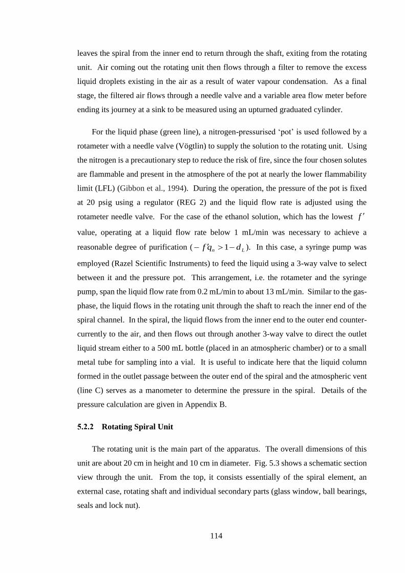
114
leaves the spiral from the inner end to return through the shaft, exiting from the rotating
unit. Air coming out the rotating unit then flows through a filter to remove the excess
liquid droplets existing in the air as a result of water vapour condensation. As a final
stage, the filtered air flows through a needle valve and a variable area flow meter before
ending its journey at a sink to be measured using an upturned graduated cylinder.
For the liquid phase (green line), a nitrogen-pressurised ‘pot’ is used followed by a
rotameter with a needle valve (Vögtlin) to supply the solution to the rotating unit. Using
the nitrogen is a precautionary step to reduce the risk of fire, since the four chosen solutes
are flammable and present in the atmosphere of the pot at nearly the lower flammability
limit (LFL) (Gibbon et al., 1994). During the operation, the pressure of the pot is fixed
at 20 psig using a regulator (REG 2) and the liquid flow rate is adjusted using the
rotameter needle valve. For the case of the ethanol solution, which has the lowest
value, operating at a liquid flow rate below 1 mL/min was necessary to achieve a
reasonable degree of purification ( Ln dqf −− 1 ). In this case, a syringe pump was
employed (Razel Scientific Instruments) to feed the liquid using a 3-way valve to select
between it and the pressure pot. This arrangement, i.e. the rotameter and the syringe
pump, span the liquid flow rate from 0.2 mL/min to about 13 mL/min. Similar to the gas-
phase, the liquid flows in the rotating unit through the shaft to reach the inner end of the
spiral channel. In the spiral, the liquid flows from the inner end to the outer end counter-
currently to the air, and then flows out through another 3-way valve to direct the outlet
liquid stream either to a 500 mL bottle (placed in an atmospheric chamber) or to a small
metal tube for sampling into a vial. It is useful to indicate here that the liquid column
formed in the outlet passage between the outer end of the spiral and the atmospheric vent
(line C) serves as a manometer to determine the pressure in the spiral. Details of the
pressure calculation are given in Appendix B.
Rotating Spiral Unit
The rotating unit is the main part of the apparatus. The overall dimensions of this
unit are about 20 cm in height and 10 cm in diameter. Fig. 5.3 shows a schematic section
view through the unit. From the top, it consists essentially of the spiral element, an
external case, rotating shaft and individual secondary parts (glass window, ball bearings,
seals and lock nut).
f

115
Glass Window
External Case
Spiral Element
Shaft
Lock Nut
Shaft Head
Lip-seals
Ball Bearing
Ball Bearing
Gas Inlet
Gas Outlet
Liquid Inlet
Liquid Outlet
Cooling Water Outlet
Cooling Water Inlet
Figure 5.3. A section view showing the anatomy of the rotating unit. The unit is drawn inverted
relative to its orientation in the experimental rig (Figs. 5.1 and 5.2).
The external case of the rotating spiral unit is made from 316L stainless steel. This
case has six ports which are connected to external flow tubing (shown on the right hand
side of Fig. 5.3), one inlet and one outlet for each of the contacting phases and for the
cooling water. Because it is important to transfer the fluids reliably from the static
passages to the rotating spiral channel, lip seals are used (blue-coloured parts in Fig. 5.3).
These seals are made from carbon fibre-PTFE (Ceetak Sealing Solutions). Inside the
case, the seals are stacked in pairs along the shaft to form six sealed chambers (annular
gaps between the seals and passage holes located at the shaft circumference). The four
pairs in the middle guide the contacting phases (inlet and outlet for the gas and the liquid)
so that they can flow independently through passages along the shaft to the spiral element
where the contacting occurs. The remaining two pairs of seals (on the top and bottom of
the unit) allow continuous flow of cooling water through four cooling passages (not
shown in Fig. 5.3) made along the shaft to carry away the frictional heat generated due to
rotation. In this work, the spiral temperature was adjusted by varying the cooling water
flow rate and determined indirectly using the method described in MacInnes and Zambri
(2015). A brief detail of the method is presented in Appendix B.
Fluids Passage

116
Fig. 5.4 shows three pairs of seals and the described fluid transfer arrangement. As
one can see, each pair is formed by installing two seals in a T-section metal holder. To
clamp the seals in the holder, spacing washers are placed between the seal pairs. Each
washer has a groove to provide a passage for liquid leaking from the seal to drain. In
general, there is no evidence of water leakage during operation. For the gas phase, a
pressure test is made regularly after each experiment to check the seal conditions by
quantifying the rate of gas leakage. This is made by filling the gas passage by a
pressurised air. For functional seals, the gas leakage rate is typically less than a few
percent of the lowest gas flow rate used in this work.
Figure 5.4. Close-up section from Fig. 5.3 showing the relationship between the shaft passage,
the lip-seal pairs and the connection fittings.
It is clear from Figs. 5.3 and 5.4 that the shaft is a key link between the seal unit and
the spiral element. The shaft is made from 316L stainless steel and fixed inside the case
by two ball bearings (located top and bottom) supported by a lock nut to prevent vertical
movement during operation, as shown in Fig. 5.3. One of the important design parameters
of the shaft is the external surface since it affects directly the sealing performance. In this
work, this part of the shaft has been improved in relation to that used in MacInnes and
Zambri (2015). Rather than hardening the shaft by treating the native metal, here the
external surface was coated by tungsten carbide layer to a thickness of about 100 µm
(Engineering Performance Coatings).
Seal Pair
Shaft
Fluids Passage
Gas Inlet
Gas Outlet
Chambers
(annular gaps)
Holder
(T-section)
Spacing Washer
Port

117
5.2.2.1 Spiral-channel Element
The passages in the shaft transfer the contacting phases to and from the spiral
element, as shown in Fig. 5.3. In the element, the two phases are brought together in a
single spiral channel to establish the rotating spiral contacting. The element is fabricated
from polyether ether ketone (PEEK) which has excellent chemical resistance and
mechanical properties. Also, it is one of the most thermally stable polymers (Patel et al.,
2010). This ensures the stability of the element structure during the operation over the
temperature range of interest.
The underside of the element is shown in Fig. 5.5 where the spiral channel can be
seen. This channel is formed by milling the PEEK surface using a computer-controlled
milling machine, yielding a channel 1.5 mm height ( h ), 4 mm depth (W ) and 910 mm
long ( L ). The spiral path is an Archimedean spiral with a fixed distance between
adjacent revolutions of 2 mm, giving sinR = 5.57 10-4 m. In the experiments, the
spiral channel was covered with a toughened glass window (10 mm thick) which allowed
an optical access and served as a seal between the channel revolutions (Fig. 5.5). So the
fluids in the spiral channel were in contact with PEEK (from three sides) and the glass
window (underside).
Figure 5.5. Underside of the spiral element showing the outer and the inner ends of the channel
and the flow direction of the contacting phases. The green and red arrows represent the liquid
solution and air, respectively. The reservoir at the outer end (L2) shows the typical liquid level
formed during operation.

118
bT
The contacting phases transfer to and from the spiral element and hence the spiral
channel through 4 holes in the shaft head (two inlets and two outlets). Because the
element is clamped firmly to the shaft head, the phases transfer directly from these holes
to four radial passages incorporated inside the element. These radial passages, in turn,
guide the phases to and from the inner and outer ends of the spiral channel (L1, L2, V1,
and V2 in Fig. 5.5). The liquid phase is fed from the inner hole of the spiral (L1) which
is near to the centre, leaving the spiral at L2, whereas the gas is introduced from the outer
end of the channel (V2), coming out from V1. In this way, counter-current contacting in
the rotating spiral channel was established.
Operational Considerations
Having described the main components of the rotating spiral unit, the operational
considerations can be discussed now. These are the thermal steady-state of the rotating
unit and the balance of the pressure at the outer end of the spiral channel between the inlet
gas phase (V2 in Fig. 5.5) and the outlet liquid phase (L2).
Thermal Steady-State of the Rotating Unit
As described previously and shown in Fig. 5.3, ball bearings are used in the rotating
unit to support the shaft rotating mechanism. The heat generated from these bearings
under rotation is significant and can transfer through the systems, reaching the spiral
channel where the two phases contact. Moreover, the seals are additional sources of heat
generation and can augment the amount of heat transferred to the system. Such frictional
heat generation due to rotation needs a period of time to propagate through the rotating
unit (in which the spiral is placed) such that a uniform temperature distribution is reached.
Any measurements should be avoided until reaching this case of thermal steady-state
otherwise the contacting will be tested under transient conditions, which is not within the
scope of this work. Establishing a steady thermal condition was achieved by monitoring
the lower bearing temperature since it is the main source of heat and the nearest to the
spiral channel region (Fig. 5.3). The measurement was made using a thermocouple
inserted in the rotating unit with the sensing tip about 2 mm from the bearing. A reading
was taken every minute using data logging (HH309A, Omega Engineering) from the start
of the rotation until the end of each experiment. A typical variation of the bearing
temperature ( ) over time is shown in Fig. 5.6 for two different cooling-water flow
rates.

119
As one can see in Fig. 5.6, the temperature started rising rapidly just beyond t = 0
and reached a roughly steady level after about 45 min. This steady state prevailed until
the end of the experiment with about 2 °C rms (root mean square) deviation in
temperature. Such deviation is expected since in each experiment a wide range of phase
flow rates is tested and that could disturb the thermal equilibrium due to introducing the
new flow rates. Thus, one should expect that the effective temperature on the spiral for
each single test may differ by a couple of degrees or less. However, accepting the
uncertainties introduced by these fluctuations reduces the experimental time considerably
since it is not necessary to wait for 45 min after every single change made in the phase
flow rates during the experiment. Further, the current apparatus does not allow for easy
temperature control. Therefore, small temperature adjustments after changing the phase
flow rates is not expected to be a practical approach. According to that, t > 45 min is
taken as a safe rule to ensure that the rotating unit is thermally stable and ready to start
the experiments and take the measurements.
Figure 5.6. Bearing temperatures recorded at two different cooling-water flow rates.
Pressure Balance
To establish the situation where the two phases flow counter-currently side by side
inside the spiral channel, balancing the pressure at the spiral reservoir between the inlet
gas and the outlet liquid is essential. This is achieved by adjusting the inlet gas pressure
so that it balances the level of the hydrostatic pressure gained by the liquid phase
( 2221 RL ), which dictates the pressure at the spiral outer end. The level of the liquid

120
in the spiral reservoir is employed as an indicator to balance the pressure. When the
pressure of the gas becomes greater than that of the liquid phase, the level of the liquid in
the reservoir decreases, eventually allowing the gas phase to flow in the outlet pathway
of the liquid phase, as shown in Fig. 5.7 a. On the other hand, when the hydrostatic
pressure exceeds the pressure of the inlet gas phase, the liquid overflows from the
reservoir, occupying a part of the inlet gas phase pathway (Fig. 5.7 b). In this case, pre-
contacting occurs outside the spiral channel. As a consequence, the entering gas is not
free of solute which reduces the purification as illustrated in Fig. 3.6 in Chapter 3. Thus,
in practice, once the level of the rotation rate has been decided, that determines the amount
of the hydrostatic pressure, balancing the pressure is then just a matter of adjusting the
inlet gas pressure such that the level of the liquid phase is fixed at a specific position
within the reservoir. Fig. 5.7 c shows the intended situation and the other cases where
Liquidair PP and Liquidair PP .
Figure 5.7. Three different cases demonstrate the pressure balance in the outer end of the spiral.
(c) This is a typical case when
The level of the liquid is fixed in the outer
reservoir and the phases flow counter-currently.
(a) This is the case when The
level of the liquid will drop and the gas phase
flows through the liquid passage (red arrows).
(b) When , the liquid will
overflow from the reservoir and pre-contacting
will occur (green arrows).
Liquid Level
Liquid Level
Liquid Level
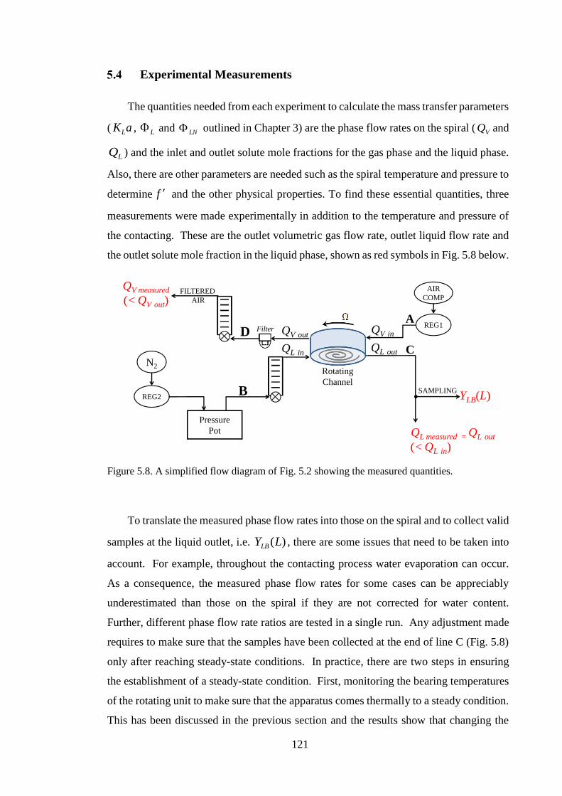
121
Rotating
Channel
Pressure
Pot
N2
REG2
A
C
D
B
REG1
AIR
COMPFILTERED
AIR
QL in
QV out
QL out
QV in
QV measured
(< QV out)
QL measured = QL out
(< QL in)
Filter
SAMPLINGYLB(L)
Experimental Measurements
The quantities needed from each experiment to calculate the mass transfer parameters
( aKL , L and LN outlined in Chapter 3) are the phase flow rates on the spiral ( VQ and
LQ ) and the inlet and outlet solute mole fractions for the gas phase and the liquid phase.
Also, there are other parameters are needed such as the spiral temperature and pressure to
determine and the other physical properties. To find these essential quantities, three
measurements were made experimentally in addition to the temperature and pressure of
the contacting. These are the outlet volumetric gas flow rate, outlet liquid flow rate and
the outlet solute mole fraction in the liquid phase, shown as red symbols in Fig. 5.8 below.
Figure 5.8. A simplified flow diagram of Fig. 5.2 showing the measured quantities.
To translate the measured phase flow rates into those on the spiral and to collect valid
samples at the liquid outlet, i.e. )(LYLB , there are some issues that need to be taken into
account. For example, throughout the contacting process water evaporation can occur.
As a consequence, the measured phase flow rates for some cases can be appreciably
underestimated than those on the spiral if they are not corrected for water content.
Further, different phase flow rate ratios are tested in a single run. Any adjustment made
requires to make sure that the samples have been collected at the end of line C (Fig. 5.8)
only after reaching steady-state conditions. In practice, there are two steps in ensuring
the establishment of a steady-state condition. First, monitoring the bearing temperatures
of the rotating unit to make sure that the apparatus comes thermally to a steady condition.
This has been discussed in the previous section and the results show that changing the
f

122
flow rate has negligible effect on the apparatus thermal status. Second, waiting enough
time for the flow and the concentration field in the spiral and the passages leading to the
sampling point (line C) to reach a steady condition for given phase flow rates.
In this work, a simplified evaporation model and an experimental procedure are
developed to address the issues discussed above since they affect directly the phase flow
rates on the spiral and the measured solute mole fractions at the liquid outlet. These
measures are discussed in detail within the relevant subsections below where the
experimental measurements are described. As pointed out previously, the determination
the spiral pressure and temperature is given in Appendix B. This left the determination
of phase flow rates and solute concentrations and these are discussed below.
Flow Rate Measurements
As shown in Fig. 5.8, the gas and liquid phase flow rates are measured during the
experiments at the end of downstream passages (the end of line C and D for the liquid
and the gas, respectively). Since air is weakly soluble in water (Sander, 2015) and is
essentially filtered at the end of line D, a water displacement method was used to
determine the gas flow rate. This was made by timed collection of the outlet gas volume
in an upturned graduated cylinder immersed in a sink of water. The conditions where the
gas was collected were within a few percent of 20 °C (laboratory ambient) and
atmospheric pressure (the liquid level in the cylinder is just few centimetres above the
sink level). In this way, the gas flow rates were documented at normal conditions. The
measurements taken for all the experiments conducted are presented chronologically in
Fig. 5.9 where rms is about 1% for the average flow rate values of 1.3, 3 and 6.2 NL/min.
For the liquid phase, four different aqueous solutions (ethanol, acetonitrile, acetone
and MEK) were tested. These solutions have different viscosities even they are intended
to be at dilute levels. For example, the 5% ethanol solution tested is about 20% more
viscous than the other solutions (Khattab et al., 2012). For this reason, the liquid
rotameter installed at the upstream passage (line B in Fig. 5.8) was employed as an
indicator rather than a measuring tool and the flow rates were measured directly at the
outlet. The measurements were carried out by collecting liquid mass for a measured time.
The collected mass was then converted to a volumetric flow rate using water density
estimated from a correlation at the ambient temperature (White, 2008). This approach
was used for all the studied systems. However, some tests for ethanol systems, as

123
0
1
2
3
4
5
6
7
8
0 10 20 30 40 50 60 70 80 90 100 110 120 130 140 150
Mea
sure
d G
as F
low
Rat
e (N
L/m
in)
Test Number
QV = 6.2 NL/min
QV = 3.0 NL/min
QV = 1.3 NL/min
mentioned, have been carried out using a syringe pump to deliver flow rates below 1
mL/min. Such flow rates are dictated by the small value of for these particular
systems ( = 0.232 and 0.651) to achieve a practical degree of purification. In this case,
the flow rate delivered by the pump was determined simply by adjusting the pump driver
speed and knowing the syringe size to determine the flow area. At the same time, the
flow rate delivered by the pump was also measured downstream by collecting mass in a
measured time. This helps in evaluating the amount of water lost on the spiral due to
evaporation as will be seen in the next section.
Figure 5.9. Gas flow rate measurements.
5.4.1.1 Simplified Evaporation Model
On the spiral, water evaporation can occur simultaneously with the solute transport
since the air used in the experiments is dry (supplied by a compressor). The implication
is that the phase flow rates measured can be underestimated than the actual flow rates on
the spiral (Fig. 5.8). Evaluating the effect of evaporation is possible by approximating
that the gas is fully saturated with water both at the exit from the spiral (at the spiral
temperature) and at the collection point (at the ambient temperature). Based on this
approximation, a simplified model was developed. The model has two purposes: first to
evaluate the effect of water evaporation in general and second to estimate the phase flow
rates on the spiral.
f
f
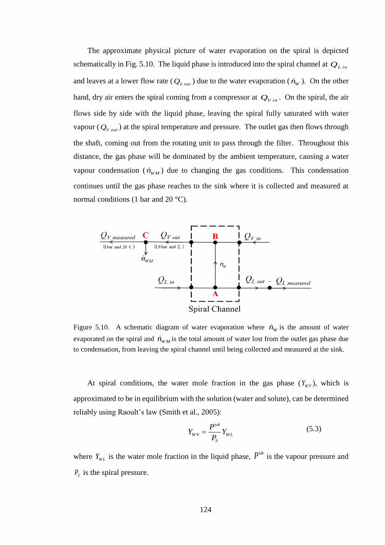
124
The approximate physical picture of water evaporation on the spiral is depicted
schematically in Fig. 5.10. The liquid phase is introduced into the spiral channel at inLQ
and leaves at a lower flow rate (outLQ ) due to the water evaporation ( Wn ). On the other
hand, dry air enters the spiral coming from a compressor at inVQ . On the spiral, the air
flows side by side with the liquid phase, leaving the spiral fully saturated with water
vapour (outVQ ) at the spiral temperature and pressure. The outlet gas then flows through
the shaft, coming out from the rotating unit to pass through the filter. Throughout this
distance, the gas phase will be dominated by the ambient temperature, causing a water
vapour condensation ( WMn ) due to changing the gas conditions. This condensation
continues until the gas phase reaches to the sink where it is collected and measured at
normal conditions (1 bar and 20 °C).
Figure 5.10. A schematic diagram of water evaporation where Wn is the amount of water
evaporated on the spiral and WMn is the total amount of water lost from the outlet gas phase due
to condensation, from leaving the spiral channel until being collected and measured at the sink.
At spiral conditions, the water mole fraction in the gas phase ( W VY ), which is
approximated to be in equilibrium with the solution (water and solute), can be determined
reliably using Raoult’s law (Smith et al., 2005):
WL
S
WV YP
PY
sat
= (5.3)
where WLY is the water mole fraction in the liquid phase, satP is the vapour pressure and
SP is the spiral pressure.

125
For a dilute solute, 1WLY and Eq. 5.3 is reduced to:
S
W VP
PY
sat
= (5.4)
In Eq. 5.4, the water vapour pressure can be calculated at the spiral temperatures using
Antoine equation (Smith et al., 2005) while the spiral pressure ( SP ) is fixed at 1.8 bara.
These conditions give a water vapour content (mole fraction) of 0.0167, 0.025 and 0.065
for a gas leaving the spiral at temperatures of 24, 30, 49 °C, respectively. The predicted
mole fractions can be used to quantify the effect of evaporation by making a mole balance
using the notation in Fig. 5.10. Thus, a balance on the water without solute (since it is
dilute) in the spiral channel gives:
For the liquid phase: WoutLLinLL nQnQn += (5.5)
For the gas phase: WW VoutVV nYQn = (5.6)
where Wn is the total molar flow rate of water evaporated along the spiral and Vn and Ln
are the molar densities of the gas and the liquid phase, respectively.
From Eqs. 5.5 and 5.6, the water volumetric flow rate can be determined in terms of the
water mole fraction in the gas phase, phase flow rates and molar densities:
L
WVoutVV
outLinLn
YQnQQ =− (5.7)
To give a sense of the amount of water evaporated with respect to the liquid flow rate fed
to the spiral, Eq. 5.7 is normalised by the inlet liquid flow rate (inLQ ):
inLL
W VoutVV
inL
L
inL
outLinL
Qn
YQn
Q
Q
Q
QQ=
=
− (5.8)
Now, it is clear from Eq. 5.8 that the amount of water evaporated in relation to the inlet
liquid flow rate is a function of temperature (implied in W VY ) and the phase flow rates for
given spiral pressure and phase densities. This equation represents the change in the
liquid phase flow rate along the spiral channel and can be used to give a rough estimate
of how the evaporation affects the liquid flow rate. Fig. 5.11 shows the results of Eq. 5.8
for air-water system, using the three gas flow rates used in the experiments (1.3, 3 and
6.2 NL/min) and liquid flow rates from 0.1 to 100 mL/min, at the three different spiral
temperatures (Table 5.1).

126
As shown in Fig. 5.11, the change in liquid flow rate due to water evaporation is
significant at the small liquid flow rate. This suggests that the studied systems with low
are the most affected by evaporation, since it is necessary for these systems to operate
at a low liquid flow rate to achieve a practical degree of purification. But the effect of
evaporation is minor for the systems with large since it allows a large liquid flow rate
to be tested. Accordingly, the ethanol systems are the most affected by evaporation (
= 0.232 and 0.651), whereas for the acetone and MEK systems ( = 3.83 and 5.5,
respectively) the effect is lower. Also, it is clear that at a given gas and liquid flow rate
the fraction of water evaporated increases as the spiral temperature increases. Thus, for
acetone system at 24 °C, the evaporation has a less effect on the liquid phase flow rate
relative to the other systems and is expected to be minor since the range of liquid flow
used to test this system is between 1 to 10 mL/min.
Additionally, the model results are compared to experimental measurements for the
case of syringe pump feeding, which was used for = 0.232 and 0.651 systems. In this
case, inLQ was determined from the pump speed and syringe size and
outLQ was
measured by collecting mass in a specific time period. Form these values, the amount of
water evaporated was determined experimentally at the three gas flow rates and compared
to the model results to check its reliability, as shown in Fig. 5.11. It is clear from the
figure that there is a scatter in the experimental measurements (symbols) in general. This
scatter could be attributed to the fact that the effective temperature on the spiral may have
been lower or higher than the values used in the evaporation model. This is consistent
with the variations in the bearing temperature measurements noticed in Fig. 5.6.
Regardless of the scatter, however, there is an obvious agreement between the model
predictions and the data. This gives a support for the validity of approximating that the
gas leaves the spiral fully saturated and suggests that the model can be used to quantify
the amount of water evaporated under these conditions.
f
f
f
f
f

127
Q
L/Q
L
QL (mL/min)
Figure 5.11. Measured (symbols) and predicted (lines) amount of water evaporated on the spiral
over different spiral temperatures and phase flow rates.

128
5.4.1.2 Spiral Inlet and Outlet Flow Rates
To this point, the above model helps in evaluating the effect of water evaporation on
the liquid flow rate and can be used also to quantify the inlet liquid flow rate (inLQ in Fig.
5.10) and the inlet and outlet gas flow rate (inVQ and
outVQ ) from the measured quantities.
According to Fig. 5.10, outVQ can be calculated by making an overall material balance
around node C:
MWmeasuredVVNoutVV nQnQn += (5.9)
where Vn and VNn are the molar densities at the spiral exit and at the collection point
(sink), respectively. WMn is the total amount of water condensed due to changing the
saturation conditions from those on the spiral (1.8 bara and TS) to normal conditions (1
bar and 20 °C) at the collection point. Saturation at the collection point is ensured by
making line D (Fig. 5.8) sufficiently long to reach ambient temperature.
WMn in Eq. 5.9 can be found by making a material balance on the water around node C,
measuredVVNWNoutVVWVWM QnYQnYn −= (5.10)
where W VY and W NY are the water mole fractions in the gas phase at the spiral and normal
conditions, respectively, and can be estimated using Raoult’s law (Eq. 5.4).
Now, substituting Eq. 5.10 in Eq. 5.9 gives outVQ as:
measuredV
W V
W N
V
VNoutV Q
Y
Y
n
nQ
)1(
)1(
−
−= (5.11)
The change in the gas phase flow rate along the spiral due to water evaporation can also
be determined:
W V
outV
inVoutVY
Q
QQ=
− (5.12)
Form outVQ (Eq. 5.11), the inlet liquid flow rate (
inLQ ) can be calculated using Eq. 5.7
where outLQ is the same as the liquid flow rate measured downstream. Accordingly, Eq.
5.7 can be re-expressed in terms of the measured liquid flow rate as:
L
WVoutVV
measuredLinLn
YQnQQ += (5.13)
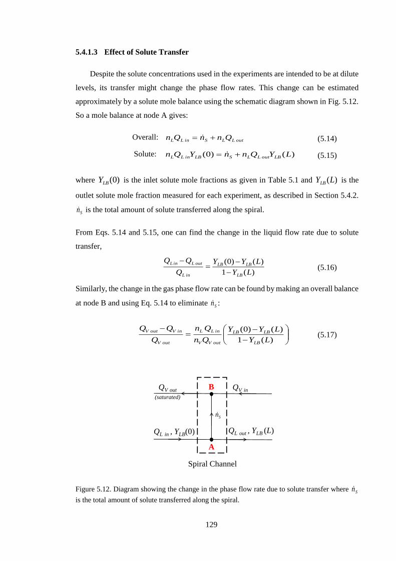
129
Spiral Channel
QV in
QL out , YLB (L)
A
B
Sn
QV out
(saturated)
QL in , YLB(0)
5.4.1.3 Effect of Solute Transfer
Despite the solute concentrations used in the experiments are intended to be at dilute
levels, its transfer might change the phase flow rates. This change can be estimated
approximately by a solute mole balance using the schematic diagram shown in Fig. 5.12.
So a mole balance at node A gives:
Overall: outLLSinLL QnnQn += (5.14)
Solute: )()0( LYQnnYQn LBoutLLSLBinLL += (5.15)
where )0(LBY is the inlet solute mole fractions as given in Table 5.1 and )(LYLB is the
outlet solute mole fraction measured for each experiment, as described in Section 5.4.2.
Sn is the total amount of solute transferred along the spiral.
From Eqs. 5.14 and 5.15, one can find the change in the liquid flow rate due to solute
transfer,
)(1
)()0(
LY
LYY
Q
LB
LBLB
inL
outLinL
−
−=
− (5.16)
Similarly, the change in the gas phase flow rate can be found by making an overall balance
at node B and using Eq. 5.14 to eliminate Sn :
−
−=
−
)(1
)()0(
LY
LYY
Qn
Qn
Q
LB
LBLB
outVV
inLL
outV
inVoutV (5.17)
Figure 5.12. Diagram showing the change in the phase flow rate due to solute transfer where Sn
is the total amount of solute transferred along the spiral.

130
5.4.1.4 Spiral Flow Rates
The flow of the phases changes with distance along the spiral channel due to both
solute transfer and water evaporation. Calculations using Eqs. 5.16 and 5.17 show that
the change in the flow rate associated with solute transfer for either phase remains less
than 7%. The effect of water evaporation is also generally small. For the gas phase, the
largest change is less than 7% (Eq. 5.12) at the highest operating temperature (49 °C).
For the liquid flow rate, however, the relative change could be very large at low liquid
flow rates (as shown in Fig. 5.11). In general, results with considerable change are
excluded from the final data based on a sensitivity analysis. This analysis was made using
the mass transfer relation (Eq. 3.32) to determine the change in the mass transfer
coefficient due to uncertainties in the measurements of flow rates. Further, the same
relation was used to quantify the effect of uncertainties in the solute concentration
measurements (discussed in the next section) and the liquid phase molar density. The
transfer of the solute along the channel changes the mean molecular mass of the liquid
phase and hence the liquid phase molar density which appears explicitly in Eq. 3.32.
Appendix C gives the details of this sensitivity analysis and shows the change in aKL
with the measurements uncertainties.
As discussed in Chapter 3, the mass transfer coefficient relation (Eq. 3.32) was
derived based on assuming constant flow rates and properties. To avoid bias in calculating
aKL , the flow rate values were taken as the average of the inlet and outlet values for each
phase. Also, the liquid molar density was taken as constant and equal to the average of
the inlet and outlet values.
Composition Measurement
The other bulk quantities required to quantify the experimental mass transfer
coefficient (Eq. 3.32) are the inlet and outlet solute mole fractions in the gas and the liquid
phase. For all the experiments, the inlet air stream was solute-free. The composition of
the feed solution was prepared using high purity raw materials and deionised water (the
specifications of these materials are given in Appendix D). This means that the inlet
solute mole fraction of the gas phase and the liquid phase are known for each test. This
left only the task of measuring the outlet solution composition, )(LYLB , to complete the
required solute mole fraction information since the outlet gas phase composition can be
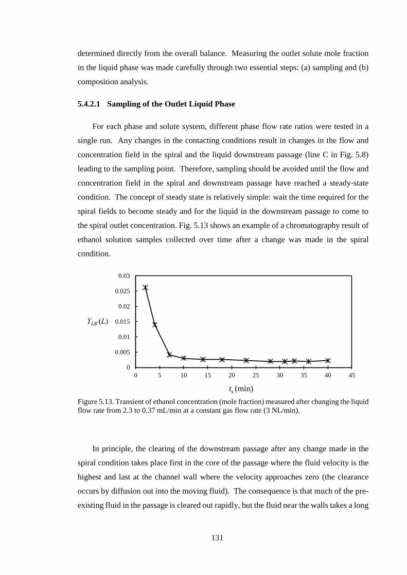
131
0
0.005
0.01
0.015
0.02
0.025
0.03
0 5 10 15 20 25 30 35 40 45
ts (min)
determined directly from the overall balance. Measuring the outlet solute mole fraction
in the liquid phase was made carefully through two essential steps: (a) sampling and (b)
composition analysis.
5.4.2.1 Sampling of the Outlet Liquid Phase
For each phase and solute system, different phase flow rate ratios were tested in a
single run. Any changes in the contacting conditions result in changes in the flow and
concentration field in the spiral and the liquid downstream passage (line C in Fig. 5.8)
leading to the sampling point. Therefore, sampling should be avoided until the flow and
concentration field in the spiral and downstream passage have reached a steady-state
condition. The concept of steady state is relatively simple: wait the time required for the
spiral fields to become steady and for the liquid in the downstream passage to come to
the spiral outlet concentration. Fig. 5.13 shows an example of a chromatography result of
ethanol solution samples collected over time after a change was made in the spiral
condition.
Figure 5.13. Transient of ethanol concentration (mole fraction) measured after changing the liquid
flow rate from 2.3 to 0.37 mL/min at a constant gas flow rate (3 NL/min).
In principle, the clearing of the downstream passage after any change made in the
spiral condition takes place first in the core of the passage where the fluid velocity is the
highest and last at the channel wall where the velocity approaches zero (the clearance
occurs by diffusion out into the moving fluid). The consequence is that much of the pre-
existing fluid in the passage is cleared out rapidly, but the fluid near the walls takes a long
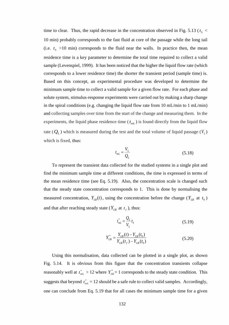
132
time to clear. Thus, the rapid decrease in the concentration observed in Fig. 5.13 ( St <
10 min) probably corresponds to the fast fluid at core of the passage while the long tail
(i.e. St >10 min) corresponds to the fluid near the walls. In practice then, the mean
residence time is a key parameter to determine the total time required to collect a valid
sample (Levenspiel, 1999). It has been noticed that the higher the liquid flow rate (which
corresponds to a lower residence time) the shorter the transient period (sample time) is.
Based on this concept, an experimental procedure was developed to determine the
minimum sample time to collect a valid sample for a given flow rate. For each phase and
solute system, stimulus-response experiments were carried out by making a sharp change
in the spiral conditions (e.g. changing the liquid flow rate from 10 mL/min to 1 mL/min)
and collecting samples over time from the start of the change and measuring them. In the
experiments, the liquid phase residence time ( mLt ) is found directly from the liquid flow
rate ( LQ ) which is measured during the test and the total volume of liquid passage ( LV )
which is fixed, thus:
L
LmL
Q
Vt = (5.18)
To represent the transient data collected for the studied systems in a single plot and
find the minimum sample time at different conditions, the time is expressed in terms of
the mean residence time (see Eq. 5.19). Also, the concentration scale is changed such
that the steady state concentration corresponds to 1. This is done by normalising the
measured concentration, )(tYLB , using the concentration before the change ( LBY at 0t )
and that after reaching steady state ( LBY at ft ), thus:
S
L
LmL t
V
Qt =*
(5.19)
)()(
)()(
0
0*
tYtY
tYtYY
LBfLB
LBLBLB
−
−= (5.20)
Using this normalisation, data collected can be plotted in a single plot, as shown
Fig. 5.14. It is obvious from this figure that the concentration transients collapse
reasonably well at *
mLt > 12 where *
LBY = 1 corresponds to the steady state condition. This
suggests that beyond *
mLt = 12 should be a safe rule to collect valid samples. Accordingly,
one can conclude from Eq. 5.19 that for all cases the minimum sample time for a given

133
0
0.2
0.4
0.6
0.8
1
1.2
0 5 10 15 20 25 30 35
*
LBY
*
mLt
flow rate must be:
LLS QVt 12 (5.21)
where LV is fixed and equals 1.6 mL and LQ is a measured quantity during the tests.
Eq. 5.21 was used throughout all experiments as a rule to collect valid samples. At each
new adjusted condition, LQ was measured first and then St (from Eq. 5.21) was
calculated to determine the minimum time to reach steady state conditions and hence a
sample could be collected and measured.
Figure 5.14. The transient experiments carried out separately for the selected phase and solute
systems (ethanol, acetonitrile, acetone and MEK) by changing LQ from approximately
10 mL/min to about 1 mL/min (except ethanol to less than 1 mL/min) and over the three gas
flow rates (1.3, 3 and 6.2 NL/min).
For each flow rate ratio tested, at least two samples of the outlet liquid were collected
using vials (Sigma-Aldrich) with sealed caps (caps with silicon/PTFE septa). The volume
of the vials used ranged between 1-3 mL, depending on the analysis method requirement.
To avoid losing solute to the atmosphere during the sampling process, the sampling outlet
(a steel tube) was immersed in the already collected liquid and was not removed until the
vial was completely filled. Further, as a precautionary step, all samples were analysed
immediately after each experiment. In this way, the time between the sampling and the
analysis was reduced and, therefore, any possible changes to the sample composition
(small leak, evaporation, unknown slow reactions) were minimised, if not avoided.

134
5.4.2.2 Liquid-phase Composition Analysis
Two instrumental analysis techniques were used to quantify the composition of the
four different solutions tested in this work. These are gas-chromatography (GC) and UV-
visible spectrophotometry. Gas-chromatography is essentially a separation technique in
which the sample mixture is vaporised and then swept by a carrier gas (creating a mobile
phase) to pass over an immiscible stationary phase (either a solid or a liquid). The
separation then, occurs because the components of the mixture tend to distribute
themselves between the two phases. Some of these components are strongly held by the
stationary phase and move slowly with the moving phase while others travel rapidly
because they are weakly retained by the stationary phase. As a result of these differences
in travelling rates, mixture components are separated into discrete groups, allowing them
to be analysed using a suitable detector (Harries et al., 2007). UV-spectrophotometry
technique, however, is different. It is based on exposing a sample (a solute in a solvent
for example) to a beam of light at a specific wavelength between 190 nm - 900 nm.
During this operation, some of the light will be absorbed by the solute and some will
transmit. The amount of light absorbed is proportional directly to the concentration of
the solute and the sample thickness in the light path (Harries et al., 2007). Based on this
principle, mixtures can be analysed qualitatively and quantitatively. For this work, Table
5.2 lists the solution type and the corresponding technique used to analyse them. As one
may note, two different types of gas-chromatography were used, GC with a thermal
conductivity detector (TCD) and GC with an ionised flame detector (FID), to analyse the
ethanol and acetonitrile solutions, respectively. The spectrophotometry, on the other
hand, was used for both acetone and 2-butanone (MEK).
Table 5.2. Summary of solution types and corresponding analysis techniques.

135
Before engaging in the analysis of the samples, a strict calibration method was
adopted to ensure the reproducibility of the instruments used in this work and hence
establishing a reliable calibration curve. This includes, for each instrument, carrying out
the calibration process three times independently (often has been made in three different
days), using a new series of standards each time. This helps to identify the precision of
the instrument and also shows clearly whether there are any errors in the preparation of
the standard samples. The results showed that the reproducibility of the instruments used,
in general, is within 1% and the data of each system could be represented by a fit with
rms deviations of about 0.9%, 1.4%, 0.4% and 0.5% for ethanol, acetonitrile, acetone and
MEK, respectively (Table 5.2). Appendix E presents the calibration details including the
measurements and the fitting functions used in this work to determine the solute
concentration.
Also, as a long term monitoring procedure, the functioning of the instruments was
checked regularly throughout the work. This was done by running standard samples (at
least three) before each run. When the instrument was not within the limit of uncertainties
determined in Table 5.2, measures had been taken to diagnose and resolve the problem.
For the sake of the completeness, the details of the methods used to analyse each
individual solution are described in the next subsections.
5.4.2.2.1 Ethanol Concentration Measurement
Gas chromatograph (GC) technique is the one of the reliable analytical methods to
quantify the ethanol concentration in aqueous solutions (Weatherly et al, 2014;
Abdulrazzaq et al., 2016). The analysis can be accomplished rapidly to a high accuracy
and precision. In this work, for example, the typical run times were just over 3 min with
uncertainties less than 1%. All the ethanol solution samples were analysed using a gas
chromatograph (Varian 3900) equipped with a thermal conductivity detector, following
the method described by Abdulrazzaq et al. (2016). The injection volume used for both
calibration and sample analysis was 0.4 µL and the injection was carried out manually
using a 1 μL syringe (SGC, Australia). The column used for all measurements was a
packed column type HAYESEP P (80-100 mesh) with an internal diameter of 3 mm and
a length of 2.08 m (Varian, USA). The GC oven and injection port temperatures were set
at 150 °C and 180 °C, respectively. The carrier gas used was nitrogen at 400 mL/min.
Finally, ethanol and water retention times were about 2 min and 0.8 min, respectively.

136
Typical chromatograms obtained using this set-up are shown in Fig. 5.15. Fig. 5.15
a and 5.15 b show the analysis of the feed composition , )0(LBY , before and after 6 hrs
experimental use where the large peak on the left represents the water and the small one
on the right is the ethanol. These two measurements were performed to evaluate the
stability of the feed composition during a run. As an experimental routine, this type of
evaluation was made throughout all the experiments. The results show that the difference
in feed composition before and after a run was always within the measurement uncertainty
(below 0.9%). Thus, the solution inlet concentration (whether supplied by a nitrogen-
pressurised ‘pot’ or a syringe pump) was fixed throughout all tests performed.
For the outlet composition, Fig. 5.15 c and Fig. 5.15 d show the analysis of two
samples. The first was sampled after running only the solution in the spiral while the
outlet gas phase (air) was off (Fig. 5.15 c) and the second was sampled after normal
operation (i.e. contacting with the gas phase). As expected, the result show no change in
the outlet composition with respect to the feed composition when the air was off whereas
a reduction in the ethanol peak size was observed (Fig. 5.15 c) when operating at normal
conditions. These two experiments demonstrate clearly that contacting of the two phases
was achieved and desorption of ethanol solute from the water into the air occurred.

137
Time (min)
Volt
age
(mV
)V
olt
age
(mV
)
Time (min)
Time (min)
Time (min)
a) Feed Composition (before a run) b) Feed Composition (after a run)
c) Outlet Composition
(outlet air off)
d) Outlet Composition
(with air)
Figure 5.15. GC-TCD chromatograms for ethanol solutions: (a) feed composition before a run,
(b) feed composition after 6 hrs experimental use, (c) outlet composition where the outlet gas
phase is off and (d) outlet composition after counter-current contacting with the gas phase.
5.4.2.2.2 Acetonitrile Concentration Measurement
For the acetonitrile solutions, all analyses were carried out using a gas chromatograph
(Perkin Elmer AutoSystem XL) supplied with ionised flame detector (FID). The analysis
method was developed by the chemistry department of the University of Sheffield. For
this ste-up, the suitable injection volume was 0.1 μL and the sample was injected using
an autosampler. The column used was a capillary column, type Alltech AT1 (30 m length
and 0.32 mm internal diameter) coated with 5 µm pure dimethylpolysiloxane. The GC
oven and the injector temperatures were set at 200 °C and 250 °C, respectively. Hydrogen
was used as a carrier gas (2.4 mL/min) and the split ratio was 20:1. The acetonitrile
retention time was approximately 1 min and that was out of 10 min of an analysis time.
Fig. 5.16 shows a typical chromatogram of an analysis with an acetonitrile peak emerging
at a retention time of 1.07 min.

138
Acetonitrile peak
Figure 5.16. A chromatogram of GC-FID showing the acetonitrile peak.
5.4.2.2.3 Acetone and MEK Concentration Measurement
For acetone and MEK solutions, UV-visible spectrophotometry was used to analyse
the samples. This technique has been successfully used for these types of solutes in
various studies (Gierczak et al., 1998; Schutze and Herrmann, 2004; Nadasdi et al., 2010).
In this work, all tests were carried out using Ultrospec 2100 pro (Amersham Biosciences)
at room temperature and ambient pressure. Disposable plastic cuvettes (semi-micro,
Fisherbrand) with a volume 1.5 mL and pathlength 1 cm were used to hold the samples
during the tests.
As a part of the procedure, the device was zeroed using a blank of deionised water
(the same source of water was used throughout the calibration and experiments) before
each single test. This isolates the effect of both the solvent (water) and the cuvette and
hence the light absorbance measured by the device is merely due to the presence of solute.
It was found that an effective absorbance could be obtained at 280 nm wavelength for
both acetone and MEK. This wavelength was fixed and used throughout the calibration
(Appendix E) and analyses. Using the same wavelength for both solutes was found to be
consistent with the literature. Schutze and Herrmann (2004) and Nadasdi et al. (2010)
reported that the difference in absorption spectrum between the two solutes is just a few
nanometres. In addition, this particular wavelength is within the acetone and MEK
absorption bands which are approximately between 230-340 nm.

139
Summary
The chapter described step by step the mass transfer experiments conducted in this
thesis. All desorption experiments were studied in a spiral channel with 1.5 mm height
( h ), 4 mm depth (W ) and 910 mm long ( L ). The operating conditions were: pressure
of 1.8 bara, rotation rate of 3200 rpm and three different temperatures (24, 30 and 49 °C).
Three different gas phase flow rates were tested (1.3, 3.0 and 6.2 NL/min) over a range
of liquid flow rates. The experimental apparatus used to collect the data was described,
including the flow network and the rotating spiral unit. The time needed to reach a thermal
steady-state was discussed along with the necessity to balance the pressure at the outer
end of the spiral between the inlet gas and the outlet liquid.
The last part of this chapter focused on the measurements of the phase flow rates and
the solute mole fraction at the liquid outlet. The effect of water evaporation and the
transfer of the solute on the phase flow rates was quantified. While the solute has a minor
effect on the phase flow rates, water evaporation can cause appreciable change in the
liquid phase flow rate along the channel especially at small LQ values. As a policy here,
data showing considerable change were rejected based on a sensitivity analysis using the
mass transfer relation (Appendix C). Furthermore, for the purpose of aKL determination,
the phase flow rates and the liquid phase molar density were taken constant and equal to
the average of the inlet and outlet. At the end of the chapter, an experimental method to
collect valid samples was discussed and the techniques used to analyse the liquid phase
composition were described.

140
Chapter Six
6 Phase and Solute Properties
Theoretical predictions using the models presented in Chapter 4 and calculations of
the experimental mass transfer coefficient using the relations in Chapter 3 require a
reliable knowledge of the phase and solute physical properties. In particular, the solute
diffusion coefficients, the density and viscosity of each phase and the solute equilibrium
distribution are required. These properties are determined in this work using either a
fundamental theory, standard empirical relations or data from the literature. This chapter
presents the method used to determine each property. The chapter is organized into two
main sections. The first section deals with the determination of solute properties while
the second section covers the details of phase properties determination.
6.1 Solute Properties
Solute Equilibrium Distribution ( f )
Determination of vapour-liquid equilibrium data using the fundamental
thermodynamic relations is possible. The modified Raoul’s law provides a realistic
description of the equilibrium behaviour of the selected solutes under the conditions of
interest. As argued in Chapter 4, the spiral pressure varies little along the channel and the
temperature is approximately uniform. So the gas phase can be treated as incompressible
(perfect). Further, water exhibits considerably non-ideal behaviour with the selected
organic solutes (Bergmann and Eckert, 1991; Sherman et al., 1996; Kojima et al., 1997),
and that is exactly the case where the law is applicable. The modified Raoult’s law is
expressed as follows:
LV YP
PY
sat
= (6.1)
where VY and LY are the solute mole fractions in the gas and liquid phase, respectively,
satP is the pure solute vapour pressure and is the activity coefficient in the liquid phase
which is a function of the temperature and LY .
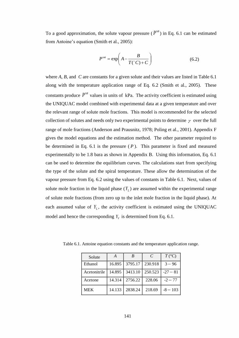
141
To a good approximation, the solute vapour pressure (satP ) in Eq. 6.1 can be estimated
from Antoine’s equation (Smith et al., 2005):
+−=
CCT
BAP
)(expsat
(6.2)
where A, B, and C are constants for a given solute and their values are listed in Table 6.1
along with the temperature application range of Eq. 6.2 (Smith et al., 2005). These
constants produce satP values in units of kPa. The activity coefficient is estimated using
the UNIQUAC model combined with experimental data at a given temperature and over
the relevant range of solute mole fractions. This model is recommended for the selected
collection of solutes and needs only two experimental points to determine over the full
range of mole fractions (Anderson and Prausnitz, 1978; Poling et al., 2001). Appendix F
gives the model equations and the estimation method. The other parameter required to
be determined in Eq. 6.1 is the pressure ( P ). This parameter is fixed and measured
experimentally to be 1.8 bara as shown in Appendix B. Using this information, Eq. 6.1
can be used to determine the equilibrium curves. The calculations start from specifying
the type of the solute and the spiral temperature. These allow the determination of the
vapour pressure from Eq. 6.2 using the values of constants in Table 6.1. Next, values of
solute mole fraction in the liquid phase ( LY ) are assumed within the experimental range
of solute mole fractions (from zero up to the inlet mole fraction in the liquid phase). At
each assumed value of LY , the activity coefficient is estimated using the UNIQUAC
model and hence the corresponding VY is determined from Eq. 6.1.
Table 6.1. Antoine equation constants and the temperature application range.
Solute A B C T (°C)
Ethanol 16.895 3795.17 230.918 3 − 96
Acetonitrile 14.895 3413.10 250.523 -27 − 81
Acetone 14.314 2756.22 228.06 -2 − 77
MEK 14.133 2838.24 218.69 -8 − 103

142
Fig. 6.1 shows the equilibrium curve calculated from Eq. 6.1 for each solute over the
relevant range of solute mole fractions and spiral temperatures. In each single plot, the
maximum LY represents the inlet solute mole fraction in the liquid phase used in the
experiments. It is clear from Fig. 6.1 that the equilibrium relation is not a strong curving
function and a linear presentation is possible, i.e. LV YfY = . To give a best estimate
of , the sum of the squared difference between the values of LY calculated from Eq.
6.1 and those from the proposed linear function ( LV YfY = ) is minimised. This gives
values of between 0.232 for ethanol system at 30 °C to 5.5 for MEK at 49 °C (as
shown in Fig. 6.1) with a maximum rms deviation of about 3%. These values are used in
this work to represent the solute equilibrium distribution for each system at a given
temperature and over the range of mole fractions of interest.
f
f

143
Figure 6.1. Solute equilibrium distribution at SP = 1.8 bara and spiral temperatures.

144
Solute Diffusion Coefficients
6.1.2.1 Diffusion Coefficient in the gas Phase
For the purpose of the determination of the gas phase diffusion coefficient, the gas
mixture is treated as a binary system of air and solute. This is reasonable since the solute
diffuses into a gas mixture consisting mostly of air with a small percent of water vapour
(at most 6 mol% which represents the saturation mole fraction at 49 °C). For binary gas
systems, there are several theoretical and semi-empirical equations in the literature for
estimating the solute diffusion coefficient ( VD ). Many of these equations are reviewed
and compared to experimental data by Poling et al. (2001). One of the most reliable and
easy to use equations is that developed by Fuller et al. (1969) (Sherwood et al., 1975;
Poling et al., 2001; Seader and Henley, 2006). This equation is used here to estimate VD
for the selected solutes in the gas phase. The equation is given below where the subscripts
‘S’ and ‘A’ refer to the solute and air, respectively:
23/13/12/1
75.1
)()(
00143.0
ASSA
V
vvPM
TD
+= (6.3)
In Eq. 6.3, VD is in cm2/s, P is in bar, T is in K and SAM can be found from the molar
mass of the solute ( SM ) and air ( AM ):
)/1()/1(
2
AS
SAMM
M+
= (6.4)
The quantities Sv and Av are the dimensionless diffusion volumes of the solute and air,
respectively. The diffusion volume of air is 19.7 and for the selected organic solutes, it
is calculated by summing the atomic diffusion volumes given in Table 6.2 (Fuller et al.,
1969). This gives solute diffusion volumes of 35.45, 33.86, 38.58 and 41.18 for ethanol,
acetonitrile, acetone and MEK, respectively.
Table 6.2. Dimensionless atomic diffusion volumes (Fuller et al., 1969).
Atom C H O N
Diffusion Volume 15.9 2.31 6.11 4.53

145
100.
.% −
=V
VV
Dexpt.
Dexpt.Dcalcdev
For each solute, the results of Eq. 6.3 are listed in Table 6.3 at the spiral pressure
(1.8 bara) and temperatures along with relevant experimental data reported in the
literature. According to Eq. 6.3, VD is proportional to PT 75.1 for a given solute. This
relation is used to convert the experimental diffusivities at the given conditions (pressure
and temperature) to those of the spiral and hence a comparison under the same conditions
with the correlation is made, i.e.:
75.1
1
2
2
1
1
2
=
T
T
P
P
D
D
V
V (6.5)
As one can see in the table below, the maximum deviation between the values
estimated from Eq. 6.3 and the corresponding experimental data is less than 6%. The
sensitivity of the numerical computation to the possible error in VD was explored. The
results showed that the largest change in the gas phase mass transfer coefficient did not
exceed 0.5%. This, perhaps, is expected since the mass transfer mechanism in the gas
phase is largely affected by the Coriolis secondary motion over the range of gas flow rates
of interest. Thus, any changes in the amount of molecular diffusion due to changes in the
diffusion coefficient are not expected to be significant.
Table 6.3. Gas-phase diffusion coefficients calculated using Eq. 6.3 at 1.8 bara and spiral
temperatures and experimental values from the literature corrected to the same conditions
using Eq. 6.5.
Solute
ST (°C) calc. 610VD expt. 610VD dev.% * Ref.
(m2/s) (m2/s)
Ethanol 30 7.11 7.50 5.5 Kwon et al.(2004)
49 7.92 8.40 5.7 Arnold (1930)
Acetonitrile 30 7.79 7.54 3.3 Poling et al. (2001)
49 8.66 8.39 3.2 Poling et al. (2001)
Acetone 24 5.93 6.04 1.8 Kwon et al.(2004)
49 6.67 6.82 2.2 Lugg (1968)
MEK 49 5.92 5.74 3.1 Lugg (1968)
*
146
6.1.2.2 Diffusion Coefficient in the Liquid Phase
The diffusion coefficient of the solute in the liquid phase ( LD ) is much smaller than
that in the gas phase and concentration-dependent (Poling et al., 2001). Most of the
literature reviewed agree that LD is difficult to estimate because of the lack of a well-
developed theory for the liquid state (Sherwood et al., 1975; Poling et al., 2001; Seader
and Henley, 2006; Bird et al., 2007). For the case of infinite dilution, however, there are
several proposed empirical equations that can estimate LD successfully for binary
systems, giving a representative diffusion coefficient over a range of solute mole fractions
up to 0.05, or perhaps 0.1 (Poling et al., 2001). The Wilke-Chang equation is widely used
and gives a reasonably good prediction of LD for dilute solutes in aqueous solutions
(Sherwood et al., 1975; Bird et al., 2007). This equation is employed here to estimate
LD for the selected solutes in water and is given as:
0.6
S
5.08
V
)(104.7
L
LL
TMD
−= (6.6)
where LD is in cm2/s, T is in K, and LM and L are the molar mass and viscosity (cP)
of the liquid phase, respectively. For water, L is estimated using a correlation given by
White (2008). This correlation is a function of temperature only and applicable for a
temperature range of 0 − 100 °C:
2
3 )(
273003.7
)(
273306.5704.1
10788.1
)sPa(ln
+
−−=
− KTKT
L (6.7)
In Eq. 6.6, SV is the molar volume of the solute (mL/mol) at its normal boiling point.
This parameter is determined by summing the atomic contribution using the values listed
in Table 6.4. This gives molar volumes of 59.2, 56.3, 74 and 96.2 mL/mol for ethanol,
acetonitrile, acetone and MEK, respectively. The other parameters required in Eq. 6.6 is
the associate factor . Wilke and Chang (1955) recommend to be 2.6 for water.
However, this value has been revised for dilute solutes in aqueous solutions in an
independent study made by Hayduk and Laudie (1974). They used data for 89 different
substances in water and found a better accuracy can be obtained from Eq. 6.6 if = 2.26.
This value is taken and fixed in all calculations made with Eq. 6.6.

147
Table 6.4. Atomic volumes (Wilke and Chang, 1955).
Atom C H O N (Doubly Bonded)
Volume (mL/mol) 14.8 3.7 7.4 15.6
The values of LD predicted by Eq. 6.6 are listed in Table 6.5. In the same table,
the results are also compared with interpolated experimental data for ethanol and acetone
at infinite dilution. As can be seen, the deviation between the predicted values and those
reported in the literature is about 10% and that is within the expected accuracy of Eq. 6.6
(Bird et al., 2007). However, there is a clear dependency of LD on the liquid phase
viscosity which appears explicitly in Eq. 6.6. In this work, the presence of the solute
increases the viscosity of the liquid phase and hence decreases LD . Thus, it should be
expected that the deviation shown in Table 6.5 will increase by some percent if one
considers LD at the inlet solute concentration. For example, LD for 5% ethanol solution
at 30 °C is 1.32 10-5 cm2/s (Pratt and Wakeham, 1974), widening the deviation to about
15% in relation to the value estimated by Eq. 6.6. This means also that LD varies along
the channel by approximately 5% (at most) in relation to the LD value at infinite dilution
(1.4 10-5 cm2/s) reported in Pratt and Wakeham (1974). Nevertheless, computation with
the 2-D model for the ethanol system shows that 15% deviation in LD leads only to a few
percent change in mass transfer coefficient. This suggests that using Wilke and Chang
equation does not lead to a significant error in the mass transfer coefficient for these
particular systems under the conditions of the experiments.

148
100.
.% −
=L
LL
Dexpt.
Dexpt.Dcalcdev
Table 6.5. Liquid-phase diffusion coefficients calculated using Eq. 6.6 at the spiral temperatures
and experimental values from the literature.
Solute
ST (°C) calc. 910LD
(m2/s)
expt. 910LD
(m2/s)
dev.% * Ref.
Ethanol 30 53.1 1.4 9.2 Pratt and Wakeham (1974)
49 36.2 2.14 10.2 Pratt and Wakeham (1974)
Acetonitrile 30 58.1 - - -
49 43.2 - - -
Acetone 24 1.15 1.27 9.2 Tyn and Calus (1975)
49 2.07 1.89 9.4 Tyn and Calus (1975)
MEK 49 1.77 - - -
*
6.2 Phase Properties
The other physical properties required in the 2-D model and WCM computations are
the density and viscosity of the contacting phases. To simplify the determination of these
properties, the conditions of the experiments at the inlet for each phase are used (i.e.
solute-free air and solution at the inlet solute mole fraction). This approximation is
justifiable since the water vapour content in the gas phase has a relatively small effect on
the density and the viscosity of air, about 4 and 6% reduction in the density and viscosity,
respectively, at 49 °C (Tsilingiris, 2008). Furthermore, the solute mole fractions remain
at a dilute level in both phases (Fig. 6.1). So the transferring of solute does not have a
strong effect on the phase physical properties, with the exception of the ethanol solution
viscosity and that will be discussed in Section 6.2.2. Details of the density and viscosity
determination for each phase are described in the following subsections.

149
Gas-phase Properties
As pointed out previously, the change in the pressure along the channel is small and
the temperature is approximately uniform. Thus, the gas phase can be treated as an ideal
gas and the density can be calculated directly:
RT
PMVV = (6.8)
where VM is the air molar mass (28.97 kg/kmol) and R is the gas constant.
For the viscosity, data reported in Kadoya et al. (1985) suggest that the air viscosity
is a function of temperature and only weakly dependent on the pressure between 1 and 25
bar and a range of temperature between 200 and 650 K. In this work, the experimental
conditions lie between these limits. It is reasonable, therefore, to estimate gas viscosity
as a function of temperature since the pressure dependence of the viscosity is negligible
at the spiral conditions. The Sutherland law is simple and gives sufficiently accurate
results for air viscosity at a temperature range from − 40 up to 500 °C (White, 2008):
+
+
=
ST
ST 15.273
15.273
2/3
0
(6.9)
where S is the Sutherland constant and 0 is the gas viscosity at 273.15 K. For air, the
values of these constants are S = 110.56 K and 0 = 1.7894 10-5 Pa s. Using Eqs. 6.8
and 6.9, the density and the viscosity of the air at the spiral pressure and temperatures can
then be calculated. These values are given in the table below.
Table 6.6. Air propetries at the spiral pressure and temperatures.
ST (°C) V (kg/m3) 510V (Pa s)
24 2.11 1.83
30 2.06 1.85
49 1.95 1.94

150
Liquid-phase Properties
For the liquid phase, the viscosity and density reported in the literature at the relevant
temperatures and inlet solute mole fraction are used in this work. This is the case for all
the studied systems except for 1.5% MEK solution because no data were found.
Alternatively, the density and viscosity of this particular solution were estimated at 49 °C
using the volume mixing rule since it is the most dilute system. The density and viscosity
of pure MEK at 49°C used in the calculation are 773 kg/m3 and 3.03 10-4 Pa s,
respectively (Habibullah et al., 2011) and those for water at the same temperature are
988.5 kg/m3 (White, 2008) and 5.56 10-4 Pa s (Khattab et al., 2012).
The calculated properties of the MEK solution, along with those for the other
solutions collected from the literature, are listed in Tables 6.7 and 6.8. The former shows
the density of the solutions at the relevant temperatures and inlet solute mole fraction and
the latter shows the values of viscosity at the same conditions. Some of these values were
taken directly and others were interpolated from the measured values. The density and
viscosity of pure water are also listed in these same tables. These values correspond to
full purification of the liquid phase and are used here to assess the maximum variation in
the density and viscosity along the channel due to solute transfer.
It is clear from Table 6.7 that the variation of the liquid phase density along the
channel is less than 2% in all cases. On the other hand, the values of the viscosity listed
in Table 6.8 show a clear sensitivity to the solute concentration. The complete removal
of the solute drops the viscosity to about 33 percent for the ethanol system at 30 °C. In
general, such drop has two effects. First, it leads to increase the diffusion coefficient
along the channel and that is estimated to be about 5% as pointed out in Section 6.1.2.2.
Second, it produces a thinner liquid layer in the spiral at a given rotation rate. MacInnes
and Zambri (2015) have shown that at the lowest liquid flow rate tested (0.2 ml/min), this
reduction in viscosity decreases the liquid layer thickness (measured at the minimum) by
approximately 18% at 3200 rpm. All these observations may affect the mass transfer and
are taken into account when it comes to discussing the results presented in Chapter 7 and
Chapter 8.

151
7.13 40178.01000)kg/m( CCT −−=
100.%
−=
L
LWdev
100.%
−=
L
LWdev
Table 6.7. Density of the studied solutions and pure water at the relevant spiral temperatures.
*
** The water density at 24 and 49 °C is estimated using a correlation given in White (2008) because they are not given in Thomas and McAllister (1957):
Table 6.8. Viscosity of the studied solutions and pure water at the relevant spiral temperatures.
*
6.3 Summary
The chapter has described the methods used to determine the physical properties of
the seven phase and solute systems studied experimentally. These properties are used
throughout this work to make model predictions and to derive values of mass transfer
coefficients from the experimental measurements. Table 6.9 below compiles all these
properties and categorises them according to solute type and spiral temperature.
Solute TS (°C) )0(LBY W (kg/m3)
(pure water) L (kg/m3)
(water+solute) dev.%* Ref.
Ethanol 30 0.05 994.0 977.7 1.67 Khattab et al. (2012)
49 0.05 983.1 965.5 1.82 Khattab et al. (2012)
Acetonitrile 30 0.03 995.7 984.9 1.10 Saleh et al.(2006)
49 0.03 988.5 976.2 1.26 Saleh et al.(2006)
Acetone 24 0.02 997.1** 986.2 1.11 Thomas and McAllister (1957)
49 0.02 988.5** 976.2 1.26 Thomas and McAllister (1957)
MEK 49 0.015 988.5** 973.0 1.59 Volume Mixing Rule
Solute TS (°C) )0(LBY 410W (Pa s)
(pure water)
410L (Pa s)
(water+solute) dev.%* Ref.
Ethanol 30 0.05 7.98 11.9 32.9 Khattab et al. (2012)
49 0.05 5.56 6.68 16.8 Khattab et al. (2012)
Acetonitrile 30 0.03 8.00 8.43 4.63 Saleh et al.(2006)
49 0.03 5.61 5.83 3.79 Saleh et al.(2006)
Acetone 24 0.02 8.99 10.33 12.72
Howard and McAllister
(1958)
49 0.02 5.56 6.32 10.70
Howard and McAllister
(1958)
MEK 49 0.015 5.56 5.51 0.9 Volume Mixing Rule

152
So
lute
MS (k
g/km
ol)
TS
(°C)
f'
DV
(m2/s)
DL
(m2/s)
ρV
(kg/m
3)µ
V (P
a s)Y
LB
(0)
µL
(Pa s)
ρL
(kg/m
3)
30
0.2
32
7.1
1 ×
10
-61
.53
× 1
0-9
2.0
61
.85
× 1
0-5
0.0
51
.19
× 1
0-3
97
7.7
49
0.6
51
7.9
2 ×
10
-62
.36
× 1
0-9
1.9
51
.94
× 1
0-5
0.0
56
.68
× 1
0-4
96
5.5
30
0.8
12
7.7
9 ×
10
-61
.58
× 1
0-9
2.0
61
.85
× 1
0-5
0.0
38
.43
× 1
0-4
98
4.9
49
1.8
48
.66
× 1
0-6
2.4
3 ×
10
-91
.95
1.9
4 ×
10
-50
.03
5.8
3 ×
10
-49
76
.2
24
1.1
55
.93
× 1
0-6
1.1
5 ×
10
-92
.11
1.8
3 ×
10
-50
.02
1.0
3 ×
10
-39
86
.2
49
3.8
36
.67
× 1
0-6
2.0
7 ×
10
-91
.95
1.9
4 ×
10
-50
.02
6.3
2 ×
10
-49
77
.5
ME
K7
2.1
49
5.5
5.9
2 ×
10
-61
.77
× 1
0-9
1.9
51
.94
× 1
0-5
0.0
15
5.5
1 ×
10
-49
73
Eth
ano
l4
6.1
Aceto
nitrile
Aceto
ne
41
.1
58
.1
Tab
le 6.9
. Ph
ysical p
roperties o
f the sev
en p
hase an
d so
lute sy
stems stu
died
experim
entally
.
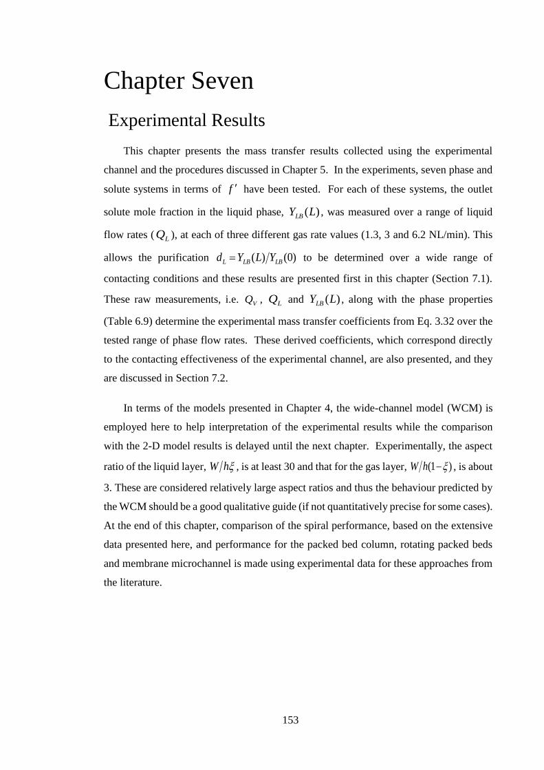
153
Chapter Seven
7 Experimental Results
This chapter presents the mass transfer results collected using the experimental
channel and the procedures discussed in Chapter 5. In the experiments, seven phase and
solute systems in terms of have been tested. For each of these systems, the outlet
solute mole fraction in the liquid phase, )(LYLB , was measured over a range of liquid
flow rates ( LQ ), at each of three different gas rate values (1.3, 3 and 6.2 NL/min). This
allows the purification )0()( LBLBL YLYd = to be determined over a wide range of
contacting conditions and these results are presented first in this chapter (Section 7.1).
These raw measurements, i.e. VQ , LQ and )(LYLB , along with the phase properties
(Table 6.9) determine the experimental mass transfer coefficients from Eq. 3.32 over the
tested range of phase flow rates. These derived coefficients, which correspond directly
to the contacting effectiveness of the experimental channel, are also presented, and they
are discussed in Section 7.2.
In terms of the models presented in Chapter 4, the wide-channel model (WCM) is
employed here to help interpretation of the experimental results while the comparison
with the 2-D model results is delayed until the next chapter. Experimentally, the aspect
ratio of the liquid layer, hW , is at least 30 and that for the gas layer, )1( −hW , is about
3. These are considered relatively large aspect ratios and thus the behaviour predicted by
the WCM should be a good qualitative guide (if not quantitatively precise for some cases).
At the end of this chapter, comparison of the spiral performance, based on the extensive
data presented here, and performance for the packed bed column, rotating packed beds
and membrane microchannel is made using experimental data for these approaches from
the literature.
f

154
Purification ( )
Effect of f
Results for measured at the intermediate gas phase flow rate (3 NL/min) for the
seven phase and solute systems are shown in Fig. 7.1. These results are presented to
highlight general trends and the effect of on the level of purification over a range of
liquid phase flow rate, approximately from 0.2 to 12 mL/min.
The first thing to note in Fig. 7.1 is that desorption has been achieved successfully
for each system, reaching approximately solute-free water ( Ld 0) for low enough liquid
flow rate. The exception is the data for = 0.232 where a liquid flow rate approaching
0.1 mL/min is required to achieve a complete removal of solute. Operating at such small
level of liquid flow rate requires an extended data sampling time. Further, it would be
associated with more uncertainties regarding layer formation ( Lmh 20 µm) therefore, it
was avoided. It is also clear from Fig. 7.1 that at a fixed the liquid phase purity
decreases, i.e. larger , as the liquid phase flow rate increases. The physical explanation
for this behaviour is that increasing the liquid flow rate decreases the residence time of
the liquid phase ( mLt ). So practically this means that less contacting time will be available
for the two phases and as a result, the purity of the liquid phase decreases as increasing
LQ . Another possible explanation is that increasing the liquid phase flow rate
excessively at fixed both and the gas phase flow rate causes a situation where the
amount of gas phase (solvent) becomes saturated with the solute. Hence, the more
increasing the liquid phase flow rate the less purity is obtained since the gas phase is not
able to remove more solute. Qualitatively, similar behaviour has been noticed for the
variation of with the liquid flow rate at the smaller and larger gas flow rates (1.3 and
6.2 NL/min). So the experimental results shown in Fig.7.1 represent a general behaviour.
The effect of on the degree of purification is also evident in Fig. 7.1. In all cases,
increasing leads to improving the purity of the liquid phase, i.e. smaller , at a given
LQ . Equivalently, as increases, the liquid flow rate that can be processed increases
at a given level of purification ( ). These two effects can be understood in terms of the
limit placed by on the phase flow rate ratio. From Chapter 2 (Eq. 2.9),
Ld
Ld
f
f
f
Ld
f
Ld
f
f Ld
f
Ld
f

155
0
0.1
0.2
0.3
0.4
0.5
0.6
0.7
0.8
0.9
1
0.1 1 10 100
QL (mL/min)
QV = 3.0 NL/min0.812
1.15
3.83
5.50
0.651
1.84
232.0=f
Repeated
Experiment)0(
)(
LB
LBL
Y
LYd =
L
LL
VVn d
Qn
Qnfqf −−=− 1 (7.1)
At the fixed solvent flow rate ( VQ = 3 NL/min), increasing increases the capacity of
this same amount of solvent to hold solute. According to Eq. 7.1, therefore, a larger
amount of LQ can be treated at a given as increases or purer liquid phase (has
smaller ) can be produced at a given LQ without violating the equation (inequality)
in either case.
Figure 7.1. Purification measured at VQ = 3 NL/min over a range of LQ values for the seven
phase and solute systems. The other contacting parameters are spiral pressure of 1.8 bara and
rotation rate of 3200 rpm. The shaded circles are repeated experiments at the same conditions.
Effect of Gas-phase Flow Rate
The results for all gas flow rates are shown in Fig. 7.2 and plotted for each value
separately. In each single plot, the values are presented as a function of LQ for each
of the three gas phase flow rates (1.3, 3, and 6.2 NL/min). The solution of the wide-
channel model at the corresponding conditions is also shown in the plots using the
properties determined in Chapter 6 (Table 6.9). The symbols are the experimental points
and the shaded dashed lines are the model calculations where the lighter shade
corresponds to the larger value of VQ .
f
Ld f
Ld
f
Ld

156
dL
Figure 7.2. Measured purification ( Ld ) at the three fixed gas flow rates over a range of liquid
flow (symbols). The shaded dashed curves are the predictions of the wide channel model (the
lighter shade corresponds to the larger value of the gas phase flow rate).

157
The effect of the liquid phase flow rate has been discussed in the preceding section
and, again, it is clear that for each system ( ) increasing LQ decreases the purity of the
liquid phase (larger ) because mLt decreases. In terms of the gas phase flow rate
(solvent phase), the effect is different. In all cases, increasing VQ at a fixed liquid flow
rate ensures adequate solvent supply to desorb more solute and hence produces a high
degree of purification. Similarly, the liquid phase flow rate for which a given purification
is achieved increases with the solvent flow rate. These general trends are captured by the
WCM. However, differences become most pronounced as both and gas phase flow
rate increase. For = 5.5 (MEK) and VQ = 6.2 NL/min, for example, the purification
in the experiment is improved many fold relative to the wide channel model. This
improvement must be a consequence of the effect of the end walls which are present in
the experimental spiral channel, but not in the WCM. As discussed in Chapter 4, the
presence of the end walls causes two main changes in relation to an infinitely wide
channel. First, the interface is not flat as that used in WCM calculations but it is curved
due to the menisci at the end walls and tilted due to the effect of gravity. The second
change is the presence of Coriolis secondary motions. These changes could explain the
differences between the experiments and the WCM model as and VQ increase.
At a given value, increasing for a fixed gas flow rate corresponds to
increasing liquid phase flow rate. The computations performed in Chapter 4 (Fig. 4.14)
demonstrate that both the liquid layer thickness and the strength of Coriolis motion
increase as LQ increases. When the liquid layer is thick, the deformation in interface
shape becomes secondary (MacInnes and Zambri, 2015) and the layer can be considered
as flat. This leaves only the effect of Coriolis motion in the experimental channel which
can enhance the mass transfer due to convection. This main difference explains the
improvement in mass transfer in the experiments relative to the model predictions as
increases above 0.812. For a fixed , the greater change in the mass transfer with gas
flow rate for the experiments is also consistent with effects of Coriolis motion, but this
time in the gas phase. The pattern of the gas phase Coriolis motion has been computed
and shown in Chapter 4 (Fig. 4.17) at conditions close to those used in the experiments.
As pointed out there, this motion occupies most of the channel and is stronger than that
in the liquid side. As increasing the gas phase flow rate, the Coriolis motion becomes
f
Ld
f
f
f
Ld f
f
f

158
more effective since the term responsible for producing this motion (i.e. VV w2 )
becomes larger. Accordingly, as observed in Fig. 7.2, an increasingly improved
purification is found in the experiments relative to the model predictions as VQ increases.
Purification Factor ( nqf − )
Plotting the measured purification as a function of nqf − places the results in the
context of the purification function developed in Chapter 3 (Eq. 3.51). So a direct check
whether the experimental data follow the common trends shown in Fig. 3.5 or not is
possible. Fig. 7.3 shows all of the experimental points plotted in this way along with the
purification function for the mLLt values of 0.4, 0.8, 1.6, 3.2, 6.4 and 12.8. The
experimental points are plotted as circles for the three fixed gas flow rates and shaded
dark to light with increasing gas flow rate.
Figure 7.3. Variation of in terms of the purification factor ( nqf − ). Symbols are the
experimental points and solid curves are the purification function results (Eq. 3.51 with Vd = 0).
It is helpful to remind here that the dashed red curve, → mLLt in Fig. 7.3, is the
maximum separation that can be achieved at a given nqf − . This is equivalent to
achieving perfect equilibrium between the inlet liquid flow and the outlet gas flow which
requires a contactor of infinite length. As expected, all the data respect this limit imposed
Ld

159
f
by the thermodynamic equilibrium which is nL qfd += 1 and no data fall under the red
curve, i.e. purification that is impossible. Additionally, there is a clear pattern in Fig. 7.3
to the spread of data over the values of mLLt , data with larger gas flow rates (light shade
circles) tend to produce smaller mLLt .
At this stage, there is a temptation to judge the effectiveness of the contacting for any
given experimental point in terms of the value of mLLt . However, as discussed in
Chapter 3, higher purification can be achieved simply by increasing the residence time,
mLt , and this cannot be considered effective contacting since no increase in specific
throughput, L , may accompany this. The pattern observed in Fig. 7.3, i.e. the spread
out of data according to gas phase flow rate, supports this argument. At a fixed nq
( LLVV QnQn ), the residence time of the liquid phase is related inversely to the liquid
phase flow rate and hence the gas phase flow rate. Since the results clearly spread out
according to gas flow rate and hence residence time, the change in mLLt in the
experiments may be mainly due to the effect of residence time and hence contacting
effectiveness cannot be judged from the plot.
Contacting Effectiveness
Mass Transfer Coefficients
Specific throughput ( L ) is the appropriate way to judge the effectiveness of
contacting at a given nqf − . As shown in Chapter 3 in relation to Eq. 3.43, L is the
product of LL naK and a function of nqf − . Therefore, at a particular value of nqf − ,
aKL behaviour corresponds directly to that of L . The aKL values derived from the
data are plotted in Fig. 7.4 as a function of nqf − for three representative values of
(0.232, 0.812 and 3.83). The results for = 0.232 (ethanol at 30 °C), = 0.812
(acetonitrile at 30 °C) and = 3.83 (acetone at 49 °C) are plotted as triangles, diamonds
and circles, respectively. As in Fig. 7.3, the data are shaded dark to light as the level of
the gas phase flow rate increases. For comparison, the wide channel model results for the
three values and gas flow rates are also plotted and indicated as shaded dashed curves
(again the lighter shade corresponds to the larger VQ ).
f
f f
f
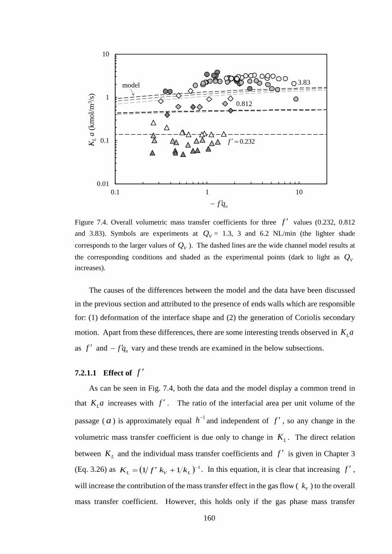
160
0.01
0.1
1
10
0.1 1 10
KL
a (
km
ol/
m3/s
)
0.812
3.83
232.0=f
model
nqf −
Figure 7.4. Overall volumetric mass transfer coefficients for three values (0.232, 0.812
and 3.83). Symbols are experiments at VQ = 1.3, 3 and 6.2 NL/min (the lighter shade
corresponds to the larger values of VQ ). The dashed lines are the wide channel model results at
the corresponding conditions and shaded as the experimental points (dark to light as VQ
increases).
The causes of the differences between the model and the data have been discussed
in the previous section and attributed to the presence of ends walls which are responsible
for: (1) deformation of the interface shape and (2) the generation of Coriolis secondary
motion. Apart from these differences, there are some interesting trends observed in aKL
as and nqf − vary and these trends are examined in the below subsections.
7.2.1.1 Effect of f
As can be seen in Fig. 7.4, both the data and the model display a common trend in
that aKL increases with . The ratio of the interfacial area per unit volume of the
passage ( a ) is approximately equal 1−h and independent of , so any change in the
volumetric mass transfer coefficient is due only to change in LK . The direct relation
between LK and the individual mass transfer coefficients and is given in Chapter 3
(Eq. 3.26) as ( ) 111
−+= LVL kkfK . In this equation, it is clear that increasing ,
will increase the contribution of the mass transfer effect in the gas flow ( Vk ) to the overall
mass transfer coefficient. However, this holds only if the gas phase mass transfer
f
f
f
f
f
f

161
0.00001
0.0001
0.001
0.01
0.1
0.1 1 10
KL
, k L
, k V
, k V
f ' (
km
ol/
m2/s
)
f '
KL
kL kV f '
kV
KL experiment
QV = 3.0 NL/min
-f 'qn = 1
coefficient makes a significant contribution. In other words, the gas-side resistance
( Vkf 1 ) is not negligible in relation to that in the liquid side ( Lk1 ) and this occurs only
if Vkf is similar in magnitude or smaller than Lk . The individual mass transfer
coefficients can be calculated using the wide channel model. This model gives
approximate values that can help to evaluate the contribution of the phases to the overall
mass transfer. The calculated coefficients are shown in Fig. 7.5 below as functions of
for the intermediate gas flow rate and nqf − = 1. The physical properties used in the
model calculations are the averages of the values listed in Table 6.9 (Chapter 6).
Figure 7.5. Wide channel model calculations showing the dependency of the mass transfer
coefficients on for 1=− nqf and VQ = 3 NL/m. Symbols are corresponding values of LK
interpolated from the experimental results.
As can be seen in Fig. 7.5, Vk is roughly uniform while Lk decreases as increases.
Both are expected since the gas phase flow rate and nqf − are fixed. So the liquid phase
flow rate must be increased as increases to maintain nqf − = 1. Any increase in the
liquid phase flow rate leads to increasing the liquid layer thickness (diffusion distance).
As a result, Lk decreases with . Comparing the contribution of the individual
coefficients, Lk remains larger than the increasing value of Vkf up to about = 4. So,
clearly, Vkf appears to have an appreciable effect on LK over this range of the data.
f
f
f
f
f
f

162
Beyond = 4, the decrease in Lk value continues but remains modest below Vkf up
to the maximum studied here, which is = 5.5. This also indicates that the overall
coefficient continues to be affected to some extent by Vkf at this range of (4 <
< 5.5).
The experimental values of LK for all the studied systems at VQ = 3 NL/min
and nqf − =1 are also shown in Fig. 7.5 (solid circle symbols). These values have
been determined from the experimental aKL results interpolated to nqf − = 1 using a
specific interfacial area ( a ) calculated from the interface shape shown in Fig. 4.3, which
is 102.1 −= ha . Comparing the experimental values to those from the wide channel
model, the same pattern observed in Fig. 7.4 is revealed, as expected. Mass transfer in the
experiments becomes increasingly more effective compared to the model results as
increases, which corresponds to increasing LQ at fixed VQ and nqf − . This behaviour
is again due to the convective effect of Coriolis motion in the liquid and the gas phase
which can increase the contribution of both individual coefficients to LK .
The results shown in Fig. 7.5 are for the intermediate VQ and nqf − = 1. At the
higher and lower experimental gas phase flow rates the picture is the same, although
the value for which LV kkf = is somewhat reduced for the higher value of VQ
and somewhat increased for the lower gas phase flow rate. Additionally, the general
behaviour is not considerably change for other values of nqf − . Based on the analysis
made in Fig. 7.5, therefore, it should be clear that the increasing aKL with observed
in Fig. 7.4 is essentially because increases the effect of Vk . A plot of L would
show exactly the same pattern of improvements with as that observed for aKL at a
given nqf − . This is clear since L differs from aKL only by the value of the nqf −
function, )ln()1( nnn qfqfqf −+ , and the liquid phase molar density ( Ln ), according to
Eq. 3.43. The function is fixed for a given value of nqf − and Ln is roughly constant
(Table 6.9). Accordingly, L also increases with at given nqf − and VQ values.
f
f f
f f
f
f
f
f
f
f
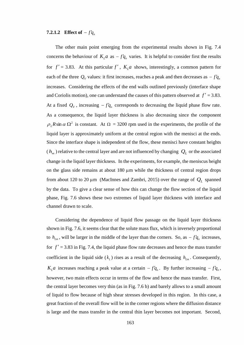
163
7.2.1.2 Effect of nqf −
The other main point emerging from the experimental results shown in Fig. 7.4
concerns the behaviour of aKL as nqf − varies. It is helpful to consider first the results
for = 3.83. At this particular , aKL shows, interestingly, a common pattern for
each of the three VQ values: it first increases, reaches a peak and then decreases as nqf −
increases. Considering the effects of the end walls outlined previously (interface shape
and Coriolis motion), one can understand the causes of this pattern observed at = 3.83.
At a fixed VQ , increasing nqf − corresponds to decreasing the liquid phase flow rate.
As a consequence, the liquid layer thickness is also decreasing since the component
2sin RL is constant. At = 3200 rpm used in the experiments, the profile of the
liquid layer is approximately uniform at the central region with the menisci at the ends.
Since the interface shape is independent of the flow, these menisci have constant heights
( mh ) relative to the central layer and are not influenced by changing LQ or the associated
change in the liquid layer thickness. In the experiments, for example, the meniscus height
on the glass side remains at about 180 m while the thickness of central region drops
from about 120 to 20 m (MacInnes and Zambri, 2015) over the range of LQ spanned
by the data. To give a clear sense of how this can change the flow section of the liquid
phase, Fig. 7.6 shows these two extremes of liquid layer thickness with interface and
channel drawn to scale.
Considering the dependence of liquid flow passage on the liquid layer thickness
shown in Fig. 7.6, it seems clear that the solute mass flux, which is inversely proportional
to Lmh , will be larger in the middle of the layer than the corners. So, as nqf − increases,
for = 3.83 in Fig. 7.4, the liquid phase flow rate decreases and hence the mass transfer
coefficient in the liquid side ( Lk ) rises as a result of the decreasing Lmh . Consequently,
aKL increases reaching a peak value at a certain nqf − . By further increasing nqf − ,
however, two main effects occur in terms of the flow and hence the mass transfer. First,
the central layer becomes very thin (as in Fig. 7.6 b) and barely allows to a small amount
of liquid to flow because of high shear stresses developed in this region. In this case, a
great fraction of the overall flow will be in the corner regions where the diffusion distance
is large and the mass transfer in the central thin layer becomes not important. Second,
f f
f
f

164
μm180=mh
μm20=Lmhμm120=Lmh
μm180=mh
Liquid Layer Gas Layer
Glass side
(a) QL = 12 mL/min (b) QL = 0.28 mL/min
the strength of Coriolis motion decreases as a result of decreasing the liquid phase flow
rate. Thus, an effective Coriolis convection in the corner regions is not to be expected.
As direct consequence of these two effects, the liquid phase mass transfer coefficient
drops at large nqf − values as most of the liquid phase flows in the corner regions where
the mass transfer is poor (large diffusion distance associated with weak Coriolis
convection). Further, it is clear in Fig. 7.4, again for = 3.83, that the position of the
peak shifts to larger nqf − as VQ increases. At larger VQ , a particular value of LQ leads
to a larger nqf − value. This suggests that there is a certain liquid phase flow rate,
and hence liquid layer thickness, that determines the peak. It is known from the
hydrodynamic study of MacInnes and Zambri (2015) and the computational results
shown in Chapter 4 (Fig. 4.17) that the gas flow rate does not greatly affect the liquid
layer thickness. So it should be expected that the liquid flow rate must be the same at the
peak regardless of the gas flow rate.
Figure 7.6. Liquid layer thickness at the minimum point ( Lmh ) and the meniscus height at the
glass side ( mh ) measured by MacInnes and Zambri (2015) at liquid phase flow rates correspond
to the maximum and the minimum liquid flow rate used in the current work.
Another behaviour observed in Fig. 7.4 is that for the other values of , the same
pattern (i.e. rise and fall in mass transfer coefficient with increasing nqf − ) is not evident.
Perhaps, this is because that the other systems are less affected by the variation
in the liquid layer thickness and hence LQ . This was the case for = 0.232 and 0.812
f
f
f

165
0.0001
0.001
0.01
0.1
0.01 0.1 1 10 100
k L ,
k Vf
' (k
mo
l/m
2/s
)
kL
kV f '
wide-channel calculations
QV = 3.0 NL/min232.0=f
83.3=f
812.0=f
nqf −
at nqf − = 1 according to the wide-channel results shown in Fig. 7.5. A similar analysis
can be made over the range of nqf − which covers the range of the experiments. This is
shown in Fig. 7.7 for the three representative values of shown in Fig. 7.4. For each
phase and solute system, the physical properties listed in Table 6.9 (Chapter 6) are used
in the WCM calculations. As can be seen clearly in the figure, the individual liquid phase
mass transfer coefficient ( Lk ) affects, in general, the overall coefficient at large , but
it diminishes as decreasing . This supports the idea that the small values of
have an overall coefficient that is less affected by Lk over the experimental range of
nqf − . Thus, a pronounced peak might not be expected at = 0.232 and 0.812. Similar
behaviour to that just described for = 0.232, 0.812 and 3.83 is found for = 0.651,
1.15 and 5.5, which are shown in Fig. 7.8. Again, a clear peak is observed only for the
largest value of , although = 1.15 data may capture the tailing off from peak.
Figure 7.7. Variation of individual mass transfer coefficients with the purification factor for
infinitely wide channel. Solid lines are values for the three in Fig. 7.4 at VQ = 3 NL/min.
f
f
f f
f
f f
f f
f
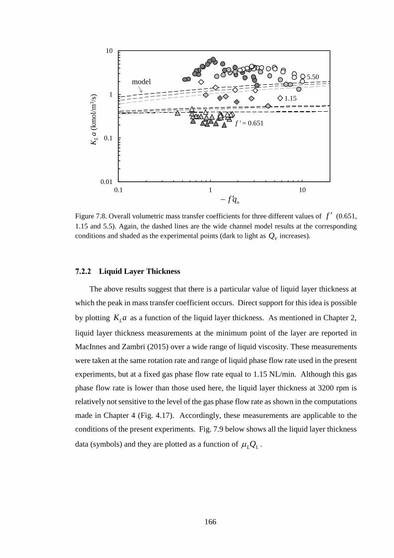
166
0.01
0.1
1
10
0.1 1 10
KL
a (
km
ol/
m3/s
)
f ' = 0.651
1.15
5.50
nqf −
model
Figure 7.8. Overall volumetric mass transfer coefficients for three different values of (0.651,
1.15 and 5.5). Again, the dashed lines are the wide channel model results at the corresponding
conditions and shaded as the experimental points (dark to light as VQ increases).
Liquid Layer Thickness
The above results suggest that there is a particular value of liquid layer thickness at
which the peak in mass transfer coefficient occurs. Direct support for this idea is possible
by plotting aKL as a function of the liquid layer thickness. As mentioned in Chapter 2,
liquid layer thickness measurements at the minimum point of the layer are reported in
MacInnes and Zambri (2015) over a wide range of liquid viscosity. These measurements
were taken at the same rotation rate and range of liquid phase flow rate used in the present
experiments, but at a fixed gas phase flow rate equal to 1.15 NL/min. Although this gas
phase flow rate is lower than those used here, the liquid layer thickness at 3200 rpm is
relatively not sensitive to the level of the gas phase flow rate as shown in the computations
made in Chapter 4 (Fig. 4.17). Accordingly, these measurements are applicable to the
conditions of the present experiments. Fig. 7.9 below shows all the liquid layer thickness
data (symbols) and they are plotted as a function of LLQ .
f

167
0.01
0.10
0.0001 0.001 0.01
hLm (mm)
LQL (Pa s mL/min)
QV = 1.15 NL/min
L= 0.67 cP (water)
L= 5.5 cP (60% glycerol)
L= 42 cP (Emim EtSO4)
L= 62 cP (88% glycerol)
06.153/1 )(103.562.0)( −−−= LLLLLm QQh
Figure 7.9. Correlation for liquid layer thickness as a function of LLQ for the experimental
channel and 3200 rpm rotation rate. Data are reported in MacInnes and Zambri (2015).
As can be seen, the data collapse well even though there is a difference of about two
orders of magnitude between the lowest and highest viscosity tested in that work.
Essentially, plotting the data against the parameter LLQ eliminates the difference in
viscosity between the tested fluids since any decrease in viscosity will need an increase
in the liquid flow rate to produce the required shear stresses to maintain a given liquid
layer thickness (MacInnes and Zambri, 2015). In this way, representing the data by a
single correlation is possible and this is indicated as a solid line in Fig. 7.9 (in terms of
Lmh and LLQ in the units given in the axis labels). This function enables the liquid layer
thickness for each experimental point in the present work to be determined using the
measured liquid phase flow rate for that point and the corresponding viscosity value from
Table 6.9. Additionally, it has been demonstrated in the previous section (Figs. 7.4 and
7.8) that aKL has a significant dependency on . This can be removed approximately
by normalising the overall mass transfer coefficient by so faKL instead of aKL is
plotted against Lmh determined from the correlation in Fig. 7.9. Fig. 7.10 shows these
results where explicitly the relation between the overall mass transfer coefficient and
liquid layer thickness for all the seven systems at the three different gas phase flow rates
can be seen.
f
f

168
0.1
1
10
10 100
KL
a /
f ' (
km
ol/
m3/s
)
hLm (m)
NL/min3.1=VQ
NL/min0.3=VQ
NL/min2.6=VQ
Figure 7.10. All data for normalised overall volumetric mass transfer coefficient plotted as a
function of liquid layer thickness.
Interestingly, the above figure shows that the data for the most part cluster together
revealing a common peak, an approximately at a liquid layer thickness of around 80 to
90 m for these phase and solute properties and this particular channel under rotation rate
of 3200 rpm. The data that deviate (in particular, those at large Lmh which lie right above
the clustered points) correspond to systems with = 0.232, 0.812 and 1.15. As one may
note in Table 6.9, these values are achieved with relatively low temperatures and
hence have relatively large values of viscosity. Viscosity for acetone at 24 °C ( = 1.15)
and for ethanol at 30 °C ( = 0.232), for example, are about double the typical viscosity
level and that for acetonitrile at 30 °C ( = 0.812) is about 50% larger than typical. At
a constant centrifugal body force and fixed layer thickness, such high viscosities
correspond to low liquid flow rates (Fig. 7.9). Accordingly, the Coriolis motion in the
liquid layer are further damped for these systems due to decreasing the liquid phase flow
rates. Thus, these systems might have aKL values which are affected by the mass
transfer processes in the liquid side at different Lmh and hence a shift in peak position.
The effect of viscosity could be augmented by the level of the gas phase flow rate since
these points collected at VQ = 6.2 NL/min. The strength of Coriolis secondary motion in
the gas phase increase with VQ and consequently this changes the relative contribution of
the indivudal mass transfer coefficents ( Vkf and Lk ) to aKL . In this case, it must be
expected that the experimental points at the largest VQ will have Vkf shifted upwards
f
f
f
f
f

169
from what is shown in Fig. 7.7, increasing at these points the impact of Lk on the overall
coefficients which is essential to determine the peak.
Despite the deviation in some data, the peak observed in Fig. 7.10 demonstrates
clearly the flexibly of rotating spiral contactor to operate at the optimum aKL by varying
only the liquid phase flow rate, independent of the gas phase flow rate. This likely
indicates that the optimum aKL can always be adjusted to occur at the optimum nqf −
by varying only the gas phase flow rate, thus simultaneously optimum contactor size and
optimum usage of solvent can be achieved.

170
Performance Comparison
Up to this point, the mass transfer characteristics of the experimental spiral have been
demonstrated over different solute properties and a range of phase flow rates. These mass
transfer data can be used now to assess the performance of rotating spiral contacting
relative to alternative gas-liquid counter-current contacting approaches. The parameter
used to judge the contacting performance is the total specific throughput. This parameter
has been presented in Chapter 3 (Eq. 3.47) and defined as the volume flow rate of the
phase being treated (the gas phase for absorption or the liquid phase for desorption)
divided by the passage volume of the contactor used. So higher specific throughput
means a smaller contactor size is required to produce the same throughput at the same
degree of purification or, equally, means for the same contactor size a higher throughput
can be achieved at a given purification.
The two different categories of contactors discussed in Chapter 2 are considered in
this comparison: the parallel-flow and the dispersed-phase contactors. For the former,
the data reported by Adiche (2018) for desorption of acetone-water-N2 system using a
membrane microchannel contactor are considered. For the latter, data for the conventional
packed column, which is commonly used in industry, and the rotating packed bed, which
has emerged recently as a proposed way of improving mass transfer by using enhanced
body force, are used. Houston and Walker (1950) reported mass transfer data for the
packed bed column over a wide range of both gas and liquid flow rates. Similar to the
experiments done here, they studied the mass transfer of different solutes having different
between air and water contacting counter-currently. For the rotating packed bed,
mass transfer of different solutes using different packing types have been studied by many
authors and again for the same phase system (water-air) and over a range of gas and liquid
flow rates. This includes studies carried out by Liu et al. (1996), Chen and Liu (2002),
Lin et al. (2004), Lin and Chien (2008), Chiang et al. (2009) and Hsu and Lin (2012). All
these studies are summarised in Table 7.1 where the values of void fraction ( ) and
solute equilibrium distribution ( ) are given. The values of listed are needed to
convert the volumetric mass transfer values from a column or bed basis to a flow passage
basis. The values of are taken from equilibrium information in the papers and are
needed to calculate the total specific throughput values from the reported mass transfer
coefficients.
f
f
f

171
Table 7.1. Parameters and conditions for the packed column, rotating packed bed and membrane
microchannel assembled from literature.
Reference Solute ( f ) T (°C ) Packing
void
fraction
Mode
Packed Column Data
Houston
& Walker
(1950)
ethanol (0.322)
methanol (0.282)
ammonia (1.08)
acetone (2.52)
27 Raschig
rings 0.72 absorption
Rotating Packed Bed Data
Liu et al.
(1996) ethanol (0.220) 20
rectangular
solids 0.53 desorption
Chen &
Liu (2002)
isopropyl alcohol (0.612)
acetone (2.37)
ethyl acetate (7.47)
25 beads 0.40 absorption
Lin et al.
(2004)
isopropyl alcohol (0.612)
ethyl acetate (7.47) 25 wire mesh 0.96 absorption
Lin &
Chien
(2008)
ethanol (0.290)
acetone (2.37)
ethyl acetate (7.47)
25 wire mesh
blades 0.99 absorption
Chiang et
al. (2009) ethanol (0.389) 30 wire mesh 0.94 absorption
Hsu & Lin
(2012)
methanol (0.275)
1-butanol (0.663) 25
wire mesh
blades 0.99 absorption
Membrane Microchannel Data
Adiche
(2018) Acetone (1.77) 23 - 0.39 desorption
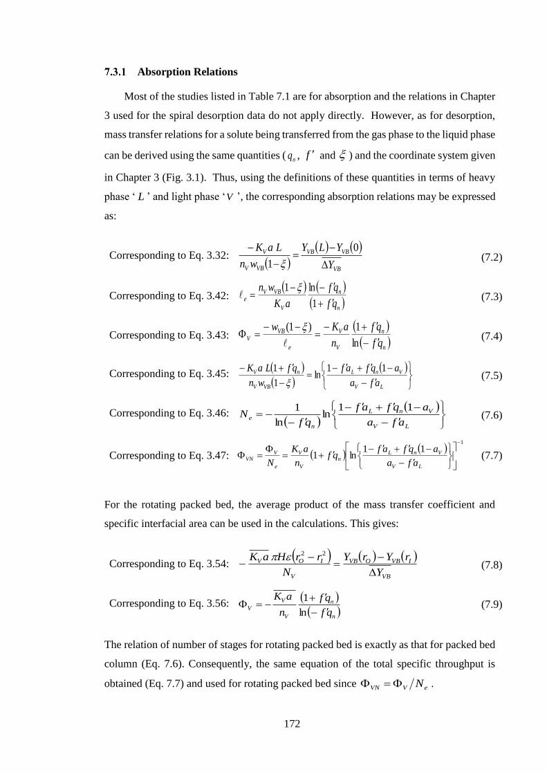
172
( )
( )1
11ln1
−
−
−+−+=
=
LV
VnLn
V
V
e
VVN
afa
aqfafqf
n
aK
N
Absorption Relations
Most of the studies listed in Table 7.1 are for absorption and the relations in Chapter
3 used for the spiral desorption data do not apply directly. However, as for desorption,
mass transfer relations for a solute being transferred from the gas phase to the liquid phase
can be derived using the same quantities ( nq , and ) and the coordinate system given
in Chapter 3 (Fig. 3.1). Thus, using the definitions of these quantities in terms of heavy
phase ‘ L ’ and light phase ‘V ’, the corresponding absorption relations may be expressed
as:
For the rotating packed bed, the average product of the mass transfer coefficient and
specific interfacial area can be used in the calculations. This gives:
The relation of number of stages for rotating packed bed is exactly as that for packed bed
column (Eq. 7.6). Consequently, the same equation of the total specific throughput is
obtained (Eq. 7.7) and used for rotating packed bed since eVVN N= .
f
Corresponding to Eq. 3.32: ( )
( ) ( )
VB
VBVB
VBV
V
Y
YLY
wn
LaK
−=
−
− 0
1 (7.2)
Corresponding to Eq. 3.42: ( ) ( )
( )n
n
V
VBVe
qf
qf
aK
wn
+
−−=
1
ln1 (7.3)
Corresponding to Eq. 3.43: ( )
( )n
n
V
V
e
VBV
qf
qf
n
aKw
−
+−=
−−=
ln
1)1(
(7.4)
Corresponding to Eq. 3.45: ( )( )
( )
−
−+−=
−
+−
LV
VnL
VBV
nV
afa
aqfaf
wn
qfLaK 11ln
1
1
(7.5)
Corresponding to Eq. 3.46: ( )
( )
−
−+−
−−=
LV
VnL
n
eafa
aqfaf
qfN
11ln
ln
1 (7.6)
Corresponding to Eq. 3.47: (7.7)
Corresponding to Eq. 3.54: ( ) ( ) ( )
VB
IVBOVB
V
IOV
Y
rYrY
N
rrHaK
−=
−−
22 (7.8)
Corresponding to Eq. 3.56: ( )
( )n
n
V
V
Vqf
qf
n
aK
−
+−=
ln
1 (7.9)
173
Normalised Specific Throughput
For absorption, Eq. 7.7 can now be used to calculate the total specific throughput and
hence a comparison of results for absorption and desorption is possible, although this
requires two adjustments. First, the volumetric flow rate used in the specific throughput
for absorption is inherently greater than that for desorption. This is due to the large
difference between the densities of the gas and the liquid phases. Such difference in
specific throughput can be adjusted easily by using molar flow rate rather than volumetric
flow rate per passage size. This means multiplying the specific throughput by the phase
molar density, i.e. VNVn and LNLn . Secondly, the increasing aKL and hence
specific throughput with for desorption can be adjusted approximately by dividing
LNLn by (as for aKL in Fig. 7.10). For absorption, such adjustment is not needed
since aKV is less sensitive to , provided that the gas phase mass transfer coefficient
dominates the overall coefficient. This can be seen in the relation between and :VK
( ) 11
−+= LVV kfkK (Eq. 3.26). So the final normalised total specific throughputs
allowing comparisons across different approaches, mass transfer modes and conditions
are VNVn (absorption) and fn LNL (desorption).
To make the comparison, the values of the total specific throughput are calculated
from Eqs. 3.47 and 7.7 using the reported flow rates and the mass transfer coefficients in
the case of the packed columns, rotating packed beds and membrane. Additionally, the
removal of the solute is taken to be 90 % ( = = 0.1) which fixes the number of
equilibrium stages in the total specific throughput relations (Eqs. 3.46 and 7.6).
Experimental points violating the limit placed by on the phase flow rate ratio (e.g.
Eq. 7.1 for desorption) simply means achieving this particular degree of separation is not
possible. Thus, data with nqf − less than Ld−1 = 0.9 (for desorption) or nqf − greater
than )1(1 Va− = 1/0.9 (for absorption) cannot be plotted, as occurs with all of desorption
data of Liu et al. (1996) and some data for spiral and other approaches.
f
f
f
f
Ld Va
f

174
Comparison Results
Fig. 7.11 shows the normalised total specific throughput plotted against nqf − for
desorption and nqf −1 for absorption. In this way, the abscissa measures solvent usage
relative to the minimum possible for both absorption and desorption, placing the two
operations on the same basis.
The rotating spiral data are indicated as red circles in Fig. 7.11 and cluster
relatively in a coherent manner as a function of the purification factor. The grey diamonds
are the Houston and Walker (1950) data for a static packed column. Unlike a rotating
spiral, the packed column data tend to spread broadly in both the vertical and horizontal
direction. Horizontally, the data extending far beyond nqf −1 = 10 simply indicates that
an excessive amount of solvent (liquid phase) is used relative to the throughput of the
processed gas phase. The spread of data in the vertical direction, on the other hand, is
essentially a consequence of the gas flow rate used which affects directly the specific
throughput. (The larger the gas phase flow rate the higher the specific throughput.)
However, the highest points for the packed column are near the limit of the theoretical
gas flow rate producing flooding (Houston and Walker,1950). As discussed in Chapter
2, the maximum allowable throughput of the gas phase in a packed column is normally
determined by the flooding behaviour which is one of the inherent limitations in this
approach. So the highest data of the packed bed shown in Fig. 7.11 are probably the
maximum performance that can be achieved. Comparing to the rotating spiral channel,
it is clear that the total specific throughput of the spiral is about three to four times larger
than that for packed bed in the expected region of optimum operation which is around
nqf − between 2 and 4.

175
Figure 7.11. Total specific throughput based on a mole flow rate determined from experimental
data for the rotating spiral, packed column, rotating packed beds and membrane microchannel
over different phase flow rate, contacting conditions and mass transfer modes. Data for the packed
bed, rotating packed bed and membrane are from the references listed in Table 7.1.
For rotating packed beds, the data are shown as squares with different shading.
Similar to the packed column, these data extend to large nqf −1 , with some
experimental points at phase flow rates ratio well above 100. This corresponds to over
a one-hundred fold increase in the amount of solvent flow rate at a particular specific
throughput and hence an excessive use of solvent flow rate. Over the large range of
nqf −1 , a pronounced increase in the rotating packed bed performance can be observed
for some data (Chiang et al., 2009 and Chen and Liu, 2002) relative to that for the packed
bed. This improvement may be attributed to the enhanced body force which allows
operation at higher gas phase velocity in relation to the static packed bed. This effect can
be seen clearly in the plot of Sherwood correlation shown in Chapter 2 (Fig. 2.4) which
shows the possible enhancement in gas phase velocity as increasing the acceleration term
(i.e. replacing g by 2R ). However, interestingly, such performance drops and becomes
comparable to the performance of the conventional packed column as flow rate ratio

176
decreases below 10. This is except for two data points of Chen and Liu (2002) which
achieve a specific throughput just 35% lower than for the rotating spiral in a range of
nqf −1 less than 10. Since all of the packed bed data in Fig. 7.11 (whether rotating or
not) are for absorption, decreasing nqf −1 corresponds to decreasing liquid phase flow
rate. As mentioned in Chapter 2, Burns and Ramshaw (1996) observed that at low liquid
flow rate the liquid phase travels through the rotating packed bed as segregated rivulets
and flying droplets rather than continuous film, leaving most of packing area not
effectively-wetted. Thus, at low liquid flow rate, one would expect that this
maldistribution becomes more pronounced and hence the contacting efficiency decreases
dramatically and becomes as that for the packed bed or even less (Lin et al. 2004). This
is consistent with the experimental study carried out by Sandilya et al. (2001) which finds
that the transfer coefficient of a conventional packed bed can be larger than that for a
rotating packed bed as a result of this liquid phase maldistribution.
For the parallel-flow contactor, the data are shown as yellow circles. These data are
for desorption of acetone from water into N2 using membrane with two meandering
channels: 3 mm for the gas phase and 100 µm for the liquid phase. While the phase and
solute system and the contacting conditions are approximately similar to those achieved
in the spiral, it is clear that the spiral data produce a larger specific throughput by a factor
of 2 at nqf − value between 2 and 4. This difference could be attributed to the presence
of the Coriolis secondary motion in rotating spiral contacting and the additional mass
transfer resistance added by membrane. These two factors must result in a better
contacting in the spiral in relation to membrane microcontactor. However, it is clear that
the performance of this contactor shows an improvement in relation to packed bed column
by about 50% at nqf − between 1 and 2.
Finally, increasing the spiral channel specific throughput can be achieved by
decreasing the channel height ( h ). As pointed out in Chapter 2, stripping distillation of
a binary system has been carried out by MacInnes et al. (2012) in a rotating spiral channel
with h = 300 µm at = 5000 rpm. The individual mass transfer coefficients have been
computed over the full range of bulk mole fraction (Ortiz-Osorio et al., 2009) and these
can be converted to specific throughput using Eqs. 3.26 and 3.47. This has been done by
calculating aKL and at dilute concentration for the more-volatile species being f

177
transferred from the liquid phase into the gas phase as for desorption process. The
experimental point of MacInnes et al (2010) is shown as a red triangle in Fig. 7.11. As
can be seen, this rough estimation gives specific throughput about 12 times greater than
that for the 1.5 mm spiral channel used in the current experiments. Thus, reducing
channel size appears to be a direct approach to improve the rotating spiral performance,
without imposing any limitations.
Summary
Measurements of desorption of four different organic solutes from water into air were
presented in this chapter over a range of water flow rates, air flow rates and solute
equilibrium distribution. The results showed that that the spiral can handle this wide
range of phase and solute systems achieving approximately solute-free water when the
appropriate flow rate ratio is chosen. These mass transfer measurements were used to
quantify the contacting effectiveness of the spiral, representing by the overall volumetric
mass transfer coefficient based on the liquid side ( aKL ). The results showed that the
contacting effectiveness increases with due to increasing the gas phase contribution
( Vkf ) to LK . Also, interestingly, it was found that the mass transfer coefficient varies
with nqf − , forming a clear peak at the three different gas phase flow rates for the large
values. This behaviour depends on the liquid phase making a significant contribution
to LK . Exploration with the wide channel model, which can compute the individual mass
transfer coefficients, suggests that LK is more affected by the individual liquid phase
mass transfer coefficient for the systems with = 3.83 and 5.5 than the other systems
with lower .
Using the liquid layer thickness measurements reported in MacInnes and Zambri
(2015) for the same channel, it was found that the peak in aKL occurs approximately at
the same liquid layer thickness (80-90 µm), independent of the gas phase flow rate. This
feature of rotating spiral contacting enables selection of gas phase flow rate to achieve
the optimum phase flow rate ratio ( nqf − ) for a given solute and, at the same time, aKL
is optimum.
f
f
f
f

178
At the end of the chapter, a comparison of spiral performance with the conventional
packed column, rotating packed bed and membrane mircochannel contactors was made.
The normalised specific throughput (molar flow rate of the treated stream divided by the
passage volume) was used as the comparison criterion, where maximum specific
throughput corresponds to minimum device volume to achieve a given separation.
Interestingly, it was found that the rotating spiral is able to operate in the appropriate
range of phase flow rate ratio and gives the highest normalised specific throughput,
demonstrating clearly the capability of this approach to produce a controlled contacting.
While the wide-channel model captures some trends of the data, considerable
differences were found due to the effect of end walls in the experimental channel. This
makes it necessary to include this effect to understand the mechanism of mass transfer in
the experimental channel. For this purpose, the 2-D computational model presented in
Chapter 4 will be used and the results are given in the next chapter.

179
Chapter Eight
8 Computational Results
This chapter is about the results obtained following the 2-D computational model
presented in Chapter 4. The chapter is divided into three main parts. The first presents
computations to compare with the experiments of MacInnes and Zambri (2015). As
pointed out, the 2-D model considers the case of a dilute solute where the mass transfer
has no appreciable effect on the phase physical properties (density and viscosity).
Therefore, the solution of the flow equations is completely independent of the species
equation and can be handled separately. This opens up the possibility of using the
hydrodynamic data reported in MacInnes and Zambri (2015) to assess the hydrodynamic
part of the model separately before taking into account any mass transfer contribution. It
is expected that such assessment would be helpful since it includes a direct comparison
based on the liquid layer thickness which is, arguably, the most important parameter in
terms of the mass transfer. The second part presents a comparison with the current mass
transfer results, in particular the purification measurements and mass transfer coefficients
presented in Chapter 7 (Figs. 7.2, 7.4 and 7.8). Finally, the chapter closes with a
parametric study. The computations made in Chapter 4 demonstrate the effect of the gas
and liquid flow rates at a fixed rotation rate. In this chapter, the focus will be on three
further important parameters: rotation rate, channel aspect ratio and the variation of both
the gas phase and liquid phase for a given phase and solute system.
8.1 Prediction of Liquid Layer Thickness
As mentioned previously, MacInnes and Zambri (2015) reported measurements of
liquid layer thickness at the minimum point of the interface profile ( Lmh ) for the air-water
system. The experiments were conducted in the same channel described in Chapter 5.
All the measurements were taken locally at the outer revolution of the channel, at a radial
position of 0R = 34 mm, over a range of conditions. Here, three sets of experiments are
considered in which the value of Lmh is measured over a range of liquid flow rate ( LQ ),
fixed gas flow rate ( VQ = 3.54 NL/min) and three different rotation rates ( =1480, 2400
and 3840 rpm). The operating conditions (pressure and temperature) for each rotation

180
rate are given in that same work and they are 2.1 bara (constant) and 307, 310 and 313 K,
respectively, for 1480, 2400, and 3840 rpm (MacInnes and Zambri, 2015). So the density
and viscosity of each phase are fully defined. Using the phase properties and values of
the contact angles used in the previous computations (Table 4.2), the interface shape is
computed individually at 0R = 34 mm for each rotation rate as described in Chapter 4
(Section 4.3). Fig. 8.1 shows the computational geometry and the computed interface
profile at the corresponding value of rotation rate. It is helpful to remember that while
the interface has a fixed shape at each rotation rate, its position and hence Lmh may change
in response to flow rates.
Now, all the parameters required to predict the minimum liquid layer thickness
( Lmh ) from the numerical solution are defined and these are:
• The geometry of the computational domains including the true shape of the
interface (Fig. 8.1).
• The flow and continuity equations for each phase (listed in Section 4.2.4).
• The suitable boundary conditions (discussed in Section 4.4).
• The phase physical properties estimated at the experimental conditions and the
other constant parameters such as sinR and .
The numerical solution of the equations, however, is not intended explicitly to track the
minimum liquid layer thickness. This is obvious since Lmh is not one of the dependent
variables. But instead the solution can determine the velocity profile in each phase and
hence LQ and VQ at a given interface position (defined by Lmh ) and pressure gradient
level ( dzdp0 ). As pointed out, VQ is fixed while LQ is varying in the set of the
experiments considered here. Thus, following the same solution approach described in
Chapter 4 (Section 4.5.5), Lmh can be predicted by only adjusting the level of dzdp0 at a
given Lmh value such that VQ calculated matches that measured experimentally while
LQ is determined from the solution. For each rotation rate, this same approach is
employed over a range of LQ covering that of the experiments. This is done with a
maximum error less than 0.5 % between the predicted and the measured gas phase flow
rate. The details of the results are discussed in the next section.

181
x
y
(a) 1480 rpm (b) 2400 rpm (c) 3840 rpm
PEEK
AirWater
Glass window
Meniscus
region
Meniscus
region
Figure 8.1. Computational geometry divided by an interface located at a particular Lmh value.
The interface is computed at radial position 0R = 34 mm for conditions typical of the
experiments: (a) T = 307 K, V = 2.41 kg/m3 and L = 994 kg/m3, (b) T = 310 K, V = 2.39
kg/m3 and L = 992.2 kg/m3 and (c) T = 313 K, V = 2.02 kg/m3 and L = 992.13 kg/m3. The
pressure for all the cases is 2.1 bara.
8.1.1 Results and Discussion
Fig. 8.2 shows the Lmh measurements (symbols) and the prediction of the 2-D model
(red curves) as a function of LQ for the three different rotation rates. The wide channel
model (WCM) results, which are shown as grey dashed curves, are also included. These
results are used here to provide the reference case of two phases separated by a flat
interface.
As can be seen in Fig. 8.2, the general behaviour is captured well by the 2-D model
and the results are in a good agreement with the experimental measurements, particularly
at =1480 and 3200 rpm. At =2400 rpm, however, the 2-D model relatively under-
predicts the minimum liquid layer thickness approximately at LQ > 3 mL/min. The inset
in Fig. 8.2 shows clearly the behaviour. This could be attributed to the experimental
scatter which is obvious in the data at this rotation rate in relation to other values and that
may lead to such difference.
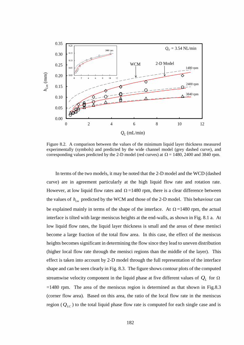
182
Figure 8.2. A comparison between the values of the minimum liquid layer thickness measured
experimentally (symbols) and predicted by the wide channel model (grey dashed curve), and
corresponding values predicted by the 2-D model (red curves) at = 1480, 2400 and 3840 rpm.
In terms of the two models, it may be noted that the 2-D model and the WCD (dashed
curve) are in agreement particularly at the high liquid flow rate and rotation rate.
However, at low liquid flow rates and =1480 rpm, there is a clear difference between
the values of Lmh predicted by the WCM and those of the 2-D model. This behaviour can
be explained mainly in terms of the shape of the interface. At =1480 rpm, the actual
interface is tilted with large meniscus heights at the end-walls, as shown in Fig. 8.1 a. At
low liquid flow rates, the liquid layer thickness is small and the areas of these menisci
become a large fraction of the total flow area. In this case, the effect of the meniscus
heights becomes significant in determining the flow since they lead to uneven distribution
(higher local flow rate through the menisci regions than the middle of the layer). This
effect is taken into account by 2-D model through the full representation of the interface
shape and can be seen clearly in Fig. 8.3. The figure shows contour plots of the computed
streamwise velocity component in the liquid phase at five different values of LQ for
=1480 rpm. The area of the meniscus region is determined as that shown in Fig.8.3
(corner flow area). Based on this area, the ratio of the local flow rate in the meniscus
region ( LCQ ) to the total liquid phase flow rate is computed for each single case and is
0.00
0.05
0.10
0.15
0.20
0.25
0.30
0.35
0 2 4 6 8 10 12
hL
m(m
m)
QL (mL/min)
WCM 2-D Model1480 rpm
2400 rpm
3840 rpm
QV = 3.54 NL/min
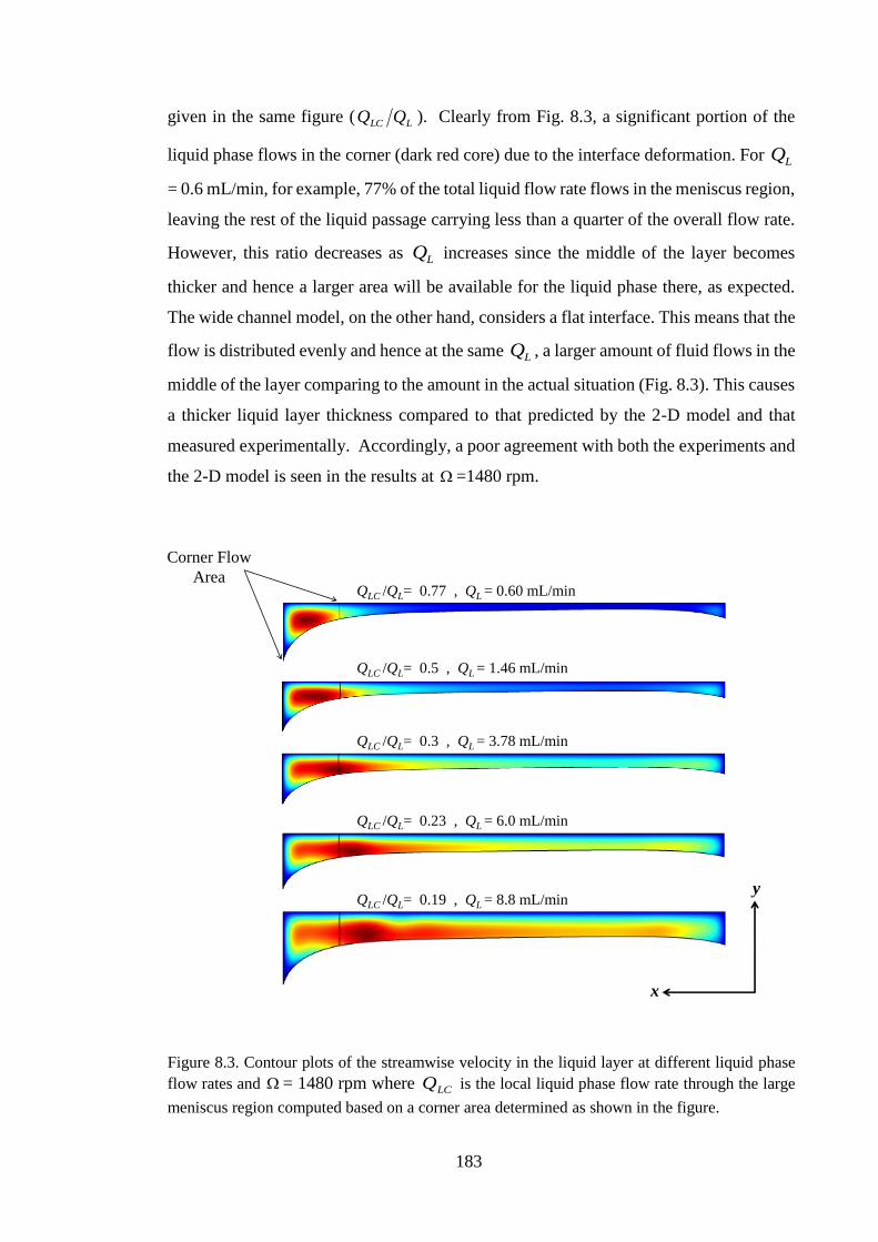
183
Corner Flow
AreaQLC /QL= 0.77 , QL = 0.60 mL/min
QLC /QL= 0.5 , QL = 1.46 mL/min
QLC /QL= 0.3 , QL = 3.78 mL/min
QLC /QL= 0.23 , QL = 6.0 mL/min
QLC /QL= 0.19 , QL = 8.8 mL/miny
x
given in the same figure ( LLC QQ ). Clearly from Fig. 8.3, a significant portion of the
liquid phase flows in the corner (dark red core) due to the interface deformation. For LQ
= 0.6 mL/min, for example, 77% of the total liquid flow rate flows in the meniscus region,
leaving the rest of the liquid passage carrying less than a quarter of the overall flow rate.
However, this ratio decreases as LQ increases since the middle of the layer becomes
thicker and hence a larger area will be available for the liquid phase there, as expected.
The wide channel model, on the other hand, considers a flat interface. This means that the
flow is distributed evenly and hence at the same LQ , a larger amount of fluid flows in the
middle of the layer comparing to the amount in the actual situation (Fig. 8.3). This causes
a thicker liquid layer thickness compared to that predicted by the 2-D model and that
measured experimentally. Accordingly, a poor agreement with both the experiments and
the 2-D model is seen in the results at =1480 rpm.
Figure 8.3. Contour plots of the streamwise velocity in the liquid layer at different liquid phase
flow rates and = 1480 rpm where LCQ is the local liquid phase flow rate through the large
meniscus region computed based on a corner area determined as shown in the figure.

184
However, as pointed out, the difference between the wide channel model and the 2-
D model becomes smaller as the liquid flow rate and the rotation rate increase (e.g. LQ
6 mL/min and =3840 rpm in Fig. 8.2). Bearing in mind the effect of the interface shape
on the liquid phase distribution, the reasons for this behaviour must be understood. As the
rotation rate increases, the interface becomes less tilted with small menisci (nearly flat)
as shown in Fig. 8.1. Add to that, the contribution of middle part of the layer becomes
larger in relation to these small menisci as the liquid flow rate increases. Hence, one can
infer that the combined effect of increasing the flow rate and the rotating rate makes the
menisci to be much less important or even negligible and thus a good agreement with the
WCM is obtained at both high rotation rate and high liquid flow rate.
8.2 Prediction of Mass Transfer Parameters
In this section, the results of the full 2-D model are compared to the experimental
measurements of the current work. For the liquid layer thickness (Fig. 8.4), the
comparison is made with Lmh values measured at a fixed radial position in the channel
with no mass transfer included. This simplifies the comparison since all needed is local
information about the interface shape at this particular radial position and physical
properties of pure air-water system, containing no solute. Here, the situation is different
and there are some aspects needed to be considered in order to make a reliable
comparison. The increasing radial position ( 0R ) with distance along a spiral channel
means that the interface shape is not constant, but varies along the channel. Fig. 8.4 shows
the interface shape computed at the inner, outer and an intermediate radial position along
the experimental channel for 3200 rpm. As can be seen in the figure, most of the liquid
layer is insensitive to the variation in 0R value with relatively small changes confined at
the lower end of the channel (glass side). So the effect is relatively modest and the
interface shape used here is calculated using the intermediate radial position (25 mm)
(Ayash and MacInnes, 2017).
Further, the value of the surface tension is taken to be that of pure water at 25 °C
(0.07 N/m). In general, two parameters affect the surface tension: the temperature and
the presence of the solute. The variation of surface tension with temperature is negligible
within the experimental range. However, the presence of solute reduces somewhat the

185
0
0.3
0.6
0.9
1.2
1.5
0 0.5 1 1.5 2 2.5 3 3.5 4
R 15 mm
R 25 mm
R 35 mm
Gas Phase
Liquid Phase
R0 = 16.5 mm
R0 = 36 mm
W (mm)
h(m
m)
rpm3200=R0 = 25 mm
R0 = 36 mm
Glass Side
water surface tension, depending on the amount and the chemical nature of the solute
(Howard and McAllister, 1958; Roemer and Leppert, 1968; Vazquez et al., 1995; Yang
et al., 1998; Rafati et al., 2010). Here, for example, the effect of adding 5% (by mole)
ethanol to water reduces the water surface tension by about 35% while the effect of adding
2% (by mole) acetone is about one half that of ethanol. The effect of the maximum
variation in surface tension on the interface shape is tested at 0R = 25 mm and it is minor
relative to the effect of 0R shown in Fig. 8.4. So taking the value of water surface tension
is suitable since the effect is small and confined at channel end. The other physical
properties used in the interface calculations are the phase densities and these values are
listed in Table 6.9. Finally, the contact angles are needed and they are taken as those
shown in Table 4.2 which are for the air and water contacting in the same experimental
channel (MacInnes and Zambri, 2015). These values are consistent with those reported
in the relevant literature (Comyn et al., 1996; Kowalczuk and Drzymala, 2016).
Figure 8.4. Interface shape computed at three different radial position corresponding to the inner,
outer and an intermediate radial position along the experimental channel where 𝜎 = 0.07 (N/m),
the phase densities are the average of the values given in Table 6.9 and the contact angles are
those given in Table 4.2.
The approximations discussed above ensure the constancy of the interface shape
along the channel. Using a fixed interface shape (red curve in Fig. 8.4), the numerical
computation allows a prediction of the local mass transfer coefficients at certain values
of bulk mole fraction level ( BY ) and bulk mole fraction gradient ( dzdYB / ). Changing
BY and dzdYB / corresponds to performing computations at different locations along the

186
channel and hence an effective transfer coefficient can be determined. However,
explorations of the effect of BY level and dzdYB / for the experimental channel suggest a
negligible effect of the choice of bulk value and gradient (Ayash and MacInnes, 2017).
So which particular values are used is only constrained by a selection that avoids the value
of mole fraction falling outside the physically-possible range of zero to unity at all
positions in the section. Since the mass transfer coefficients do not depend significantly
on the local value and gradient of bulk mole fraction, it follows that the mass transfer
coefficients are exactly constant along the channel for the above approximations and it is
unnecessary to compute mass transfer coefficients as a function of position along the
channel.
8.2.1 Purification ( )
The experimental values as a function of phase flow rates and the corresponding
WCM results were discussed in Chapter 7 in relation to Fig. 7.2. Of these results, the
values for = 1.15 and 3.83 are compared to those predicted by the 2-D numerical
model. The data for those systems are selected since they show interestingly a
pronounced difference in relation to WCM results. This difference is expected to be
mainly due to the effect of the Coriolis secondary motion. So a comparison with these
systems can clearly demonstrate the effect of this motion since it is taken into account by
the 2-D model.
Fig. 8.5 shows the values calculated for a series of computations spanning the
experimental range of gas and liquid flow rates along with the experimental results. The
experimental points are shown as open symbols (square, circle and triangle) while the
corresponding red symbols represent the prediction of the 2-D model. For reference, the
result for the wide-channel model (computed from the analytical solution given in
Chapter 4) is also included in the figure and is shown as a shaded dashed curve, the lighter
shade corresponds to the larger gas phase flow rate.
As can be seen in Fig. 8.5, the computation closely predicts the experimental
findings and it is likely that the minor deviations observed are mainly the result
of interface shape approximations and experimental uncertainties. Generally, the results
show three essential characteristics. First, the degree of purification decreases, i.e.
Ld
Ld
f
Ld
Ld

187
dL
0
0.2
0.4
0.6
0.8
1
0.1 1 10 100
Acetone, 49 C
83.3=f
QL (mL/min)
0
0.2
0.4
0.6
0.8
1Acetone, 24 C
QV = 1.3 NL/min
3.0 NL/min
6.2 NL/min
WCM
Experiment
2-D Model
15.1=f
increases, with increasing the liquid phase flow rate due to decreasing liquid phase
residence time. Second, the decreases as the gas phase flow rate increases since that
same phase can hold more solute. Finally, there is an improvement in the degree of
purification as the value of increases, which is also due to increasing the capacity of
the gas phase. All of these trends are captured by the two models but with different
quantitative success. The differences, in general, become more pronounced as both LQ
and VQ increase. Since in the wide-channel model there is no effect of secondary motion,
it is natural to suspect that this motion is what causes the considerable improvement in
the experiments and 2-D results comparing to WCM results.
Figure 8.5. Measured purification (open symbols) and the prediction of the 2-D model (red
symbols) at the three fixed gas flow rates over a range of liquid flow. The shaded dashed curves
are the prediction of the wide channel model (the lighter shade corresponds to the larger VQ
value).
Ld
f

188
It is helpful at this stage to examine briefly the role of the secondary motion, that
produces the improvement in mass transfer in relation to the WCM, using the 2-D model.
This is done by making a series of computations with and without the Coriolis terms in
the 2-D equations and solving for . The data at VQ = 6.2 NL/min for = 1.15 shown
in Fig. 8.5 are selected for demonstration and the results are plotted in Fig. 8.6. First, the
computation can be checked by reproducing the wide channel case. This is done by
imposing a flat interface and introducing symmetry boundary conditions at each end wall.
The results are shown in Fig. 8.6 as open circles and is clearly in agreement with the
analytical solution (dashed curve). Reintroducing the end wall boundary conditions and
the correct interface shape for the actual channel, but leaving out the Coriolis terms and
hence the secondary motion, leads to the results at the same gas phase flow rate shown as
cross symbols. It is clear from the results that the curving of the interface reduces the
mass transfer significantly in relation to the flat interface results, particularly at low liquid
phase flow rate. The hydrodynamic results discussed in the previous section indicate that
at a low liquid phase flow rate the middle of the layer becomes thinner and the enlarged
menisci regions divert most of the liquid flow (Fig. 8.3). Consequently, the reduction in
the degree of separation values seen in the results (crosses) at low LQ is because that the
enlarged space for liquid flow in the regions of the menisci tend to reduce mass transfer
by increasing both the characteristic streamwise velocity and diffusion length,
overcoming the opposite tendency from the thinning of the central section of the liquid
layer. Next, it proves interesting to add the Coriolis terms back into the equations, taking
the computation back to the original result over the range of liquid flow rate (red
triangles). As can be seen, the Coriolis terms in the gas phase and liquid phase bring the
mass transfer coefficient up to the original level, proving clearly the strong effect of
Coriolis secondary motion.
The series of computations shown in Fig. 8.6 decouples the effect of Coriolis
secondary motion and the interface shape and, accordingly, two main points can be
inferred, First, the Coriolis secondary motion is responsible for the difference between
the WCM and the experiments, as expected. Second, the interface curvature (cross
symbols) can decrease the mass transfer and this effect is much more pronounced as the
liquid phase flow rate decreases.
Ld f

189
0
0.2
0.4
0.6
0.8
1
0.1 1 10 100
No Coriolis Terms
Flat interface ; symmetry BCs
Coriolis terms in both phasesQV = 6.2 NL/min
dL
QL (mL/min)
Acetone, 24 C
15.1=fWCM
Experiment
nqf −
Figure 8.6. As in Fig. 8.5 for = 1.15 and VQ = 6.2 NL/min over the same range of liquid flow
rate. Red triangles are the 2-D computations, open triangles the experimental measurements and
the dashed curve the wide-channel model result. The cross and the circle symbols explore the
contribution of Coriolis motion and the interface shape to the mass transfer process in the
experimental channel.
8.2.2 Mass Transfer Coefficient
The experimental mass transfer coefficients presented in Chapter 7 (Figs. 7.4 and
7.8) are now compared with the 2-D model predictions for the intermediate gas phase
flow rate (3 NL/min). Figs. 8.7 and 8.8 below, which correspond to Figs. 7.4 and 7.8
respectively, show the experimental data (grey symbols) along with the 2-D predictions
(red symbols). Again, the WCM result is included and it is shown as a dashed curve.
In general, for the different phase and solute systems, the results in Figs. 8.7 and 8.8
show that the 2-D computation convincingly captures the mass transfer performance over
a large range of the experimental data. However, there are some differences which can
be seen clearly at some values of . It is helpful to discuss first those seen at = 3.83
(Fig. 8.7) and = 5.5 (Fig. 8.8) where the 2-D model over-predicts the mass transfer
coefficients at large values of .
f
f f
f

190
0.01
0.1
1
10
0.1 1 10
KL
a (
km
ol/
m3/s
)
0.8123.83
232.0=f
QV = 3.0 NL/min Experiment2-D Model
Interface shape with
larger meniscus height
WCM
0.01
0.1
1
10
0.1 1 10
KL
a (
km
ol/
m3/s
)
f ' = 0.651
1.15
5.50
QV = 3.0 NL/min
Interface shape with
larger meniscus height
Figure 8.7. Overall volumetric mass transfer coefficients for three values (0.232, 0.812 and
3.83) at VQ = 3.0 NL/min. The grey symbols are the experiments and the red ones are the 2-D
model predictions at the corresponding conditions. The dashed lines are the wide channel model
results.
Figure 8.8. As in Fig. 8.7 but for = 0.651, 1.15 and 5.5. Again, the dashed lines are the wide
channel model results at the corresponding conditions and the shaded symbols are the
experimental points (grey points) and the 2-D results (red points).
f
f
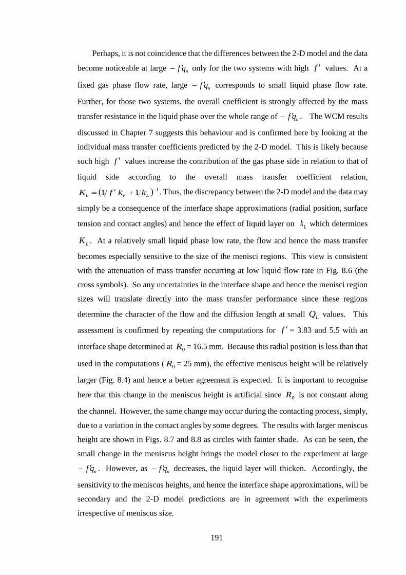
191
Perhaps, it is not coincidence that the differences between the 2-D model and the data
become noticeable at large nqf − only for the two systems with high values. At a
fixed gas phase flow rate, large nqf − corresponds to small liquid phase flow rate.
Further, for those two systems, the overall coefficient is strongly affected by the mass
transfer resistance in the liquid phase over the whole range of nqf − . The WCM results
discussed in Chapter 7 suggests this behaviour and is confirmed here by looking at the
individual mass transfer coefficients predicted by the 2-D model. This is likely because
such high values increase the contribution of the gas phase side in relation to that of
liquid side according to the overall mass transfer coefficient relation,
( ) 111
−+= LVL kkfK . Thus, the discrepancy between the 2-D model and the data may
simply be a consequence of the interface shape approximations (radial position, surface
tension and contact angles) and hence the effect of liquid layer on Lk which determines
LK . At a relatively small liquid phase low rate, the flow and hence the mass transfer
becomes especially sensitive to the size of the menisci regions. This view is consistent
with the attenuation of mass transfer occurring at low liquid flow rate in Fig. 8.6 (the
cross symbols). So any uncertainties in the interface shape and hence the menisci region
sizes will translate directly into the mass transfer performance since these regions
determine the character of the flow and the diffusion length at small LQ values. This
assessment is confirmed by repeating the computations for = 3.83 and 5.5 with an
interface shape determined at 0R = 16.5 mm. Because this radial position is less than that
used in the computations ( 0R = 25 mm), the effective meniscus height will be relatively
larger (Fig. 8.4) and hence a better agreement is expected. It is important to recognise
here that this change in the meniscus height is artificial since 0R is not constant along
the channel. However, the same change may occur during the contacting process, simply,
due to a variation in the contact angles by some degrees. The results with larger meniscus
height are shown in Figs. 8.7 and 8.8 as circles with fainter shade. As can be seen, the
small change in the meniscus height brings the model closer to the experiment at large
nqf − . However, as nqf − decreases, the liquid layer will thicken. Accordingly, the
sensitivity to the meniscus heights, and hence the interface shape approximations, will be
secondary and the 2-D model predictions are in agreement with the experiments
irrespective of meniscus size.
f
f
f

192
One might argue that the same behaviour must be seen in the other systems, i.e. the
difference between the 2-D model and the experiments increases with nqf − . This
difference, as discussed, is mainly due to the effect of the meniscus heights on Lk and
hence the overall coefficient ( LK ) which is not necessarily the case as decreases. For
= 0.812 (Fig. 8.7) and = 1.15 (Fig. 8.8), for example, the overall mass transfer
coefficients are less affected by the mass transfer in the liquid side over the nqf − range.
So any small changes in meniscus height due to using an average radial position or larger
values of surface tension and contact angles would have a small influence on the mass
transfer performance. This probably explains the agreement of the 2-D model with the
experiments for these intermediate values of . For = 0.232 (Fig. 8.7) and =
0.651 (Fig. 8.8), on the other hand, the situation is more complicated. The 2-D model
shows a gradual increase as nqf − decreases while the data are relatively less sensitive to
nqf − values over the experimental range if one considers the scatter in the data. It is
useful to remember here that these systems are for ethanol and are tested in a lower range
of liquid phase flow rate than for the other systems. For ethanol solution, the viscosity
changes by about 30% along the channel (Table 6.8) so the liquid layer thickness is no
longer constant along the channel. Further, since the experiments are carried out at small
values of liquid phase flow rates, the effect of water evaporation is expected to be strong.
This means that the liquid phase flow rate is not constant but changes significantly along
the channel. The variation in both the viscosity and flow rate of the liquid phase is not
taken into account by the 2-D model and that may lead to such anomalous behaviour
which is observed only in the data of these systems ( = 0.232 and = 0.651).
8.3 Model Parametric Analysis
The comparisons made in the previous sections show clearly the capability of the
2-D computational model to predict over a wide range of experimental conditions. So it
can be employed now to demonstrate the effect of some key parameters which have not
been tested experimentally. Three main parameters are considered in this study: rotation
rate, channel aspect ratio and different phase flow rates. To simplify the task, desorption
of acetone from water into air is taken as a reference case ( = 1.15). The properties of
this system used in the computations are given in Table 6.9. Further, the purification
f
f f
f f f
f f
f

193
factor is fixed at 1.2 (except where indicated otherwise) which is not expected to be
unreasonable value for desorption process (i.e. nqf − > 1 − ).
8.3.1 Different Rotation Rates
One of the most key parameters that this technology is based on and is fully under
external control is the rotation rate. The effect of rotation rate on the mass transfer process
is examined here by computing for a range from 1000 to 20,000 rpm with the phase flow
rates held constant at =VQ 3 NL/min and LQ = 2.2 mL/min ( nqf − = 1.2). This has
been done by adjusting both the liquid layer thickness and dzdp0 until the computed
flow rates are correct. Fig. 8.9 shows the computed streamwise velocity, secondary flow
and solute mole fraction distribution over the range of the rotation rate. In each contour
plot, the colours are shaded from blue through green to red corresponding to the range of
values from minimum to maximum. Also, it is important to note that the vector plots,
which reveal the secondary flow, are plotted with an arrow length is proportional to the
transverse velocity magnitude and using the same scale factor in all the cases for each
phase.
In general, the three main features of gas-liquid contacting can be seen clearly in the
results shown in Fig. 8.9: (1) small liquid layer with small vortices at the corners, (2)
curved interface and (3) gas phase velocity skewness with strong Coriolis motion there.
Interestingly, the rotation rate has a strong influence on these features. First of all, the
effect of increasing the rotation rate on both the interface shape and thickness of the phase
layers is evident in Fig. 8.9. As increasing both the transverse centrifugal component
( cos2R ) which determines the interface shape and the longitudinal component
( sin2R ) that drives the liquid phase increase. So in the figure, the meniscus height,
the interface tilt and the liquid layer thickness decrease simultaneously with the rotation
rate, as expected. Fig. 8.10 shows the variation of the liquid layer thickness, which is
represented by the liquid phase volume fraction ( ), over the tested range of the rotation
rate. As can be seen, decreases by approximately a factor of 10 as the rotation rate
increases from 1000 to 20,000 rpm.
Further, the effect of the rotation rate on the pattern of streamwise velocity, the
strength of the secondary motion and hence the solute mole fraction distribution is also
Ld

194
evident in Fig. 8.9. Considering the gas phase first, increasing increases the level of
the Coriolis terms in v and w equations. Accordingly, the strength of Coriolis secondary
motion and the distortion of the gas streamwise velocity profile become more pronounced
with increasing the rotation rate. In the liquid layer, on the contrary, the streamwise
velocity increases while the secondary motion diminishes as rotation rate increases. This,
perhaps, is not surprising since increasing the rotation rate is associated with a sharp
decrease in the liquid layer thickness, as shown in Fig. 8.10. As the layer thickness
decreases, the viscous effect becomes important relative to the Coriolis effect and hence
a weaker Coriolis motion generates. The order of magnitude of the viscous force relative
to the Coriolis force, known as Ekman number, is readily estimated in each phase (e.g.
Kheshgi and Scriven, 1985):
22
Ek
h
LL
= and
22 )1(Ek
−=
h
VV (8.1)
For the conditions of the computations in Fig. 8.9, the kinematic viscosity ( ) of the gas
and liquid are 8.7 10-6 and 10-6 m2/s, respectively, ranges from 105 up to 2095 rad/s
and the value of varies from 0.15 at low rotation rate to about 0.015 at the highest
(Fig.8.10). At low rotation rate, these values give LEk = 0.18 and VEk = 0.05. So,
clearly, the magnitude of viscous force to Coriolis force is higher in the liquid side than
that in the gas side. At high rotation rate, the forces become comparable in the liquid
( LEk = 0.92) while their ratio decreases by about 25 times ( VEk = 0.0018) in the gas.
According to the values of Ekman number, the secondary flow is attenuated in the liquid
side and it becomes more active in the gas as the rotation rate increases. This simple
order of magnitude analysis suggests that the magnitude of the secondary flow in relation
to streamwise velocity in the liquid side decreases with the rotation rate while it increases
in the gas phase. Numerical values that support this suggestion are shown in Fig. 8.11
where the secondary flow is represented by LV and VV (the root mean square of the
velocity in the liquid and gas phase section, respectively) and they are expressed as:
+=
+=
A
VVV
A
V
V
V
A
LLL
A
L
L
L dAvdAuA
VdAvdAuA
V 2222 1and
1 (8.2)

195
Streamwise
velocity
Secondary
motion
Solute
mole fraction
rpm4000=
Liquid
Domain
geometry
Gas
rpm2000=
GasLiquid
x
yrpm1000=1.5 mm
Phase
interface
4 m
m
Meniscus
region
Meniscus
region
GasLiquid

196
rpm8000=
GasLiquid
rpm16000=
GasLiquid
rpm20000=
GasLiquid
Streamwise
velocity
Secondary
motion
Solute
mole fraction
Domain
geometry
Figure 8.9. Numerical results (streamwise velocity, secondary flow and the solute mole fraction
distribution) for different rotation rates at VQ = 3 NL/min and LQ = 2.2 mL/min ( nqf − = 1.2).

197
0
0.02
0.04
0.06
0.08
0.1
0.12
0.14
0 4000 8000 12000 16000 20000 24000
Ω (rpm)
,
LBL wV
VBV wV
VB
Vw
VL
BL
wV
0
0.02
0.04
0.06
0.08
0.1
0.12
0.14
0.16
0.18
0 4000 8000 12000 16000 20000 24000
Ω (rpm)
Figure 8.10. Computed volume fraction of the channel occupied by the liquid phase at different
rotation rates. The flow conditions as in Fig. 8.9.
Figure 8.11. Root-mean-square velocity normalised by the streamwise velocity in each phase at
different rotation rates. The flow conditions as in Fig. 8.9.
In terms of the mass transfer, the change in the solute mole fraction distribution with
the rotation rate in Fig. 8.9 is linked directly with the changing in the interface shape. At
= 1000 rpm, for example, the top and the bottom difference in the liquid layer thickness
causes a strong difference in the streamwise liquid velocity which clearly has a strong
influence on the solute distribution. In the bottom meniscus region, where the streamwise
liquid velocity is highest, variation in the solute mole fraction is more pronounced than
the top, where liquid velocity is low. The overall solute variation along the liquid layer
has an evident effect on the solute distribution in the gas phase, a higher solute mole
fraction at the bottom and the middle than that at the top. As the rotation rate increases,
the relation between the size of the red core in the meniscus region (solute maxima) and

198
0
0.2
0.4
0.6
0.8
1
1.2
1.4
0 4000 8000 12000 16000 20000 24000
Ω (rpm)
KLa
(k
mo
l /m
3/s
)
QV = 3.0 NL/min
-f 'qn= 1.2
Acetone ( f '=1.15)
the strength of the streamwise velocity there becomes less pronounced. This is expected
since as the rotation rate increases the liquid layer becomes approximately flat,
resulting in a smaller variation in streamwise liquid velocity distribution. As a result,
approximately a symmetric solute distribution is obtained, as can be seen in the results at
8000 rpm.
Looking now at the mass transfer coefficient, the variation in mass transfer
performance with the rotation rate can be quantified. Fig. 8.12 below gives the values of
the overall volumetric mass transfer coefficients over the tested range of rotation rate.
Figure 8.12. Computed overall mass transfer coefficients against the rotation rate. The flow
conditions as in Fig. 8.9.
It is important to note that the maximum change in the interfacial area per unit
volume ( a ) associated with the change in the interface shape is about 5%. So the
behaviour shown in the above figure is essentially due to the change in LK values. The
data show clearly that the mass transfer performance increases rapidly with the rotation
rate up to about = 8000 rpm. This is attributed to the sharp decrease in the liquid layer
thickness (seen in Fig. 8.10) and the noticeable increase in the strength of the gas phase
secondary flow (Fig. 8.11) with the rotation rate which together lead to enhancing the
mass transfer in the channel. Beyond = 8000 rpm, however, the mass transfer responds
weakly to the change in the rotation rate: increasing slightly and then decreasing and thus
forming a broad peak with a maximum at around = 16,000 rpm. This is consistent with
the slow variation in both the liquid layer thickness and the secondary flow seen in Figs.

199
8.10 and 8.11, respectively, over the same range of rotation rate. As pointed out, these
parameters determined mainly the mass transfer effect. Hence, a small change in the LK
has been seen in the results at 8000 rpm with an optimum at = 16,000 rpm,
representing the best interaction of , LBL wV and
VBV wV .
The effect of the rotation rate on desorption of acetone over a range of nqf − is also
tested and the results are shown in Fig. 8.13. This is simply made by decreasing only the
liquid phase flow rate. Again, at a given nqf − , there is an improvement in mass transfer
coefficient with the rotation rate. Also, it is clear that aKL increases rapidly first between
2000 and 8000 rpm and then slowly as the rotation rate increases. These trends are similar
to those observed in Fig. 8.12 and they are attributed to the same reasons discussed above:
the decrease in the liquid layer thickness and the increase in the gas Coriolis motion.
Finally, there is a clear pattern over the range of nqf − and that is the slope of aKL curve
changes gradually with the rotation rate. This is because of the variation in the interface
shape with shown in Fig. 8.9 (domain geometry). At = 2000 rpm, the interface
shape is strongly curved with large menisci, causing decreasing the mass transfer as
nqf − increases since 11 − Ln Qqf . As the rotation increases, the interface
deformation becomes less pronounced. As a result, the solute mass transfer increases
with nqf − at > 4000 rpm since increasing nqf − reduces the liquid layer thickness
( ) and the effect of the meniscus heights is negligible.
Figure 8.13. Computed overall mass transfer coefficients for different purification factor over
different rotation rate.

200
8.3.2 Different Channel Aspect Ratio
All the experiments are made using a channel with a relatively large aspect ratio
( hW 2.5). However, this design parameter may affect the mass transfer performance
and is examined here by varying W (the channel dimension parallel to the phase layers).
Varying only W and keeping h constant ensures approximately a constant interfacial
area per unit volume (1− ha ) for the tested cases. Therefore, any changes in mass transfer
would be a direct result of changes in LK values. A channel with three different widths
are simulated: W = 1, 2 and 3 mm in addition to that used in the original design (4 mm).
The standard set of plots for each case is shown in Fig. 8.14 where = 3200 rpm and,
again, the phase flow rates are held constant at VQ = 3 NL/min and LQ = 2.2 mL/min
( nqf − = 1.2).
It is clear in Fig. 8.14 that the variation in channel width has a strong influence on
the main features of the contacting process. First of all, reducing the channel width
increases the interfacial surface force to the centrifugal force ( WC , Eq. 4.34). This
results in a more curved interface between the phases. Further, the variation in channel
width affects directly the character of the main flow and the Coriolis secondary motion
and hence the solute distribution in both phases. For the liquid phase, decreasing the
channel width results in a thicker liquid layer to conserve the mass and hence allows to
the same amount of liquid to flow in a smaller channel. So, for example, the fraction of
liquid phase ( ) increases about 2.5 times (from 0.055 to 0.137) as W decreases from 4
to 1 mm. As a direct consequence of that, the difference between the centre of the layer
and its ends becomes minor as W decreases. Thus, at W = 1 mm, the liquid phase flows
approximately evenly everywhere, causing a strong variation in streamwise liquid
velocity. The effect of streamwise liquid velocity distribution on the Coriolis motion is
evident in Fig. 8.14. Since the variation in streamwise velocity under rotation causes the
generation of the secondary flow, it is natural to see that the rotation of the smaller channel
gives rise to stronger vortices occupying most the liquid passage relative to those with
sufficiently large channel width.
It is also clear in Fig. 8.14 that the gas phase Coriolis motion becomes more active
in the smaller channel. This is mainly due to the large increase in the gas phase velocity
associated with the large reduction in the size of the passage available for the same phase.
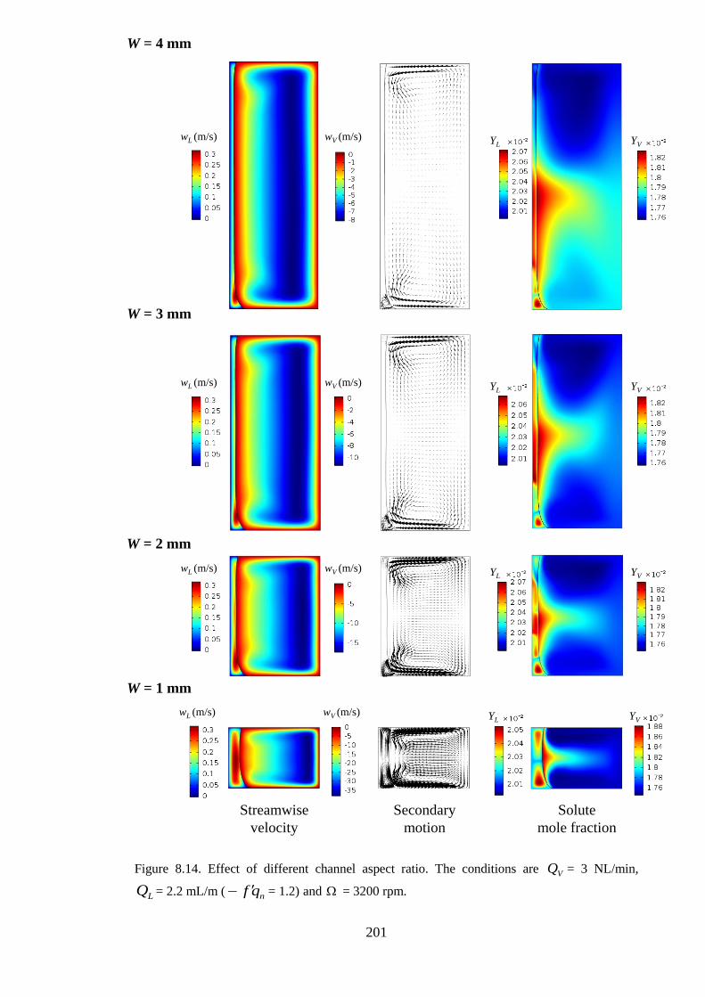
201
wV (m/s)wL (m/s) YL YV
wV (m/s)wL (m/s) YL YV
wV (m/s)wL (m/s) YVYL
wV (m/s)wL (m/s) YVYL
Streamwise
velocity
Secondary
motion
Solute
mole fraction
W = 1 mm
W = 2 mm
W = 3 mm
W = 4 mm
Figure 8.14. Effect of different channel aspect ratio. The conditions are VQ = 3 NL/min,
LQ = 2.2 mL/m ( nqf − = 1.2) and = 3200 rpm.
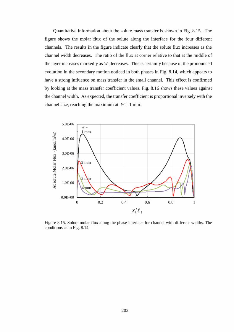
202
0.0E+00
1.0E-06
2.0E-06
3.0E-06
4.0E-06
5.0E-06
0 0.2 0.4 0.6 0.8 1
Ix
W =
1 mm
2 mm
3 mm
4 mmAb
solu
te M
ola
r F
lux
(k
mo
l/m
2/s
)
Quantitative information about the solute mass transfer is shown in Fig. 8.15. The
figure shows the molar flux of the solute along the interface for the four different
channels. The results in the figure indicate clearly that the solute flux increases as the
channel width decreases. The ratio of the flux at corner relative to that at the middle of
the layer increases markedly as W decreases. This is certainly because of the pronounced
evolution in the secondary motion noticed in both phases in Fig. 8.14, which appears to
have a strong influence on mass transfer in the small channel. This effect is confirmed
by looking at the mass transfer coefficient values. Fig. 8.16 shows these values against
the channel width. As expected, the transfer coefficient is proportional inversely with the
channel size, reaching the maximum at W = 1 mm.
Figure 8.15. Solute molar flux along the phase interface for channel with different widths. The
conditions as in Fig. 8.14.

203
0
0.5
1
1.5
2
2.5
0 1 2 3 4 5
W (mm)
KLa
(km
ol/
m2/s
)
QV = 3.0 NL/min
Acetone ( f ' = 1.15)
-f 'qn = 1.2
Figure 8.16. Values of the overall mass transfer coefficient against the channel width. The
conditions as in Fig. 8.14.
The results so far demonstrate clearly that the small channel is more efficient in
desorbing acetone from water at the flow conditions of Fig. 8.14 where nqf − = 1.2. The
effect of channel aspect ratio over a range of nqf − is also tested here by changing LQ at
VQ = 3 NL/min and = 3200 rpm. The values of the overall mass transfer coefficients
are shown in Fig. 8.17. Again, it is clear in the figure that using a small channel can
enhance mass transfer over the tested range of nqf − . At nqf − = 4, for example, the
mass transfer performance increases approximately by a factor of 2 as W decreases from
4 to 1 mm.
Another behaviour can be observed in Fig. 8.17 that there is a peak in aKL values
for W = 1 mm while for the other channel widths aKL decreases with nqf − . Looking at
the individual mass transfer coefficients, this behaviour can be understood. In Fig. 8.18,
the term akf V (dashed lines) and akL (solid lines) are plotted against nqf − for W = 1
and 2 mm. It is clear in the figure that akL is less affected by the change in the channel
width relative to akf V . Consequently, at W = 1 mm, akL becomes more dominant than
akf V , dictating the behaviour of aKL . This explains directly the different behaviour
of aKL observed at this particular channel width in Fig. 8.17. The peak in the individual
liquid phase mass transfer coefficient (red solid curve) and its effect on the overall mass
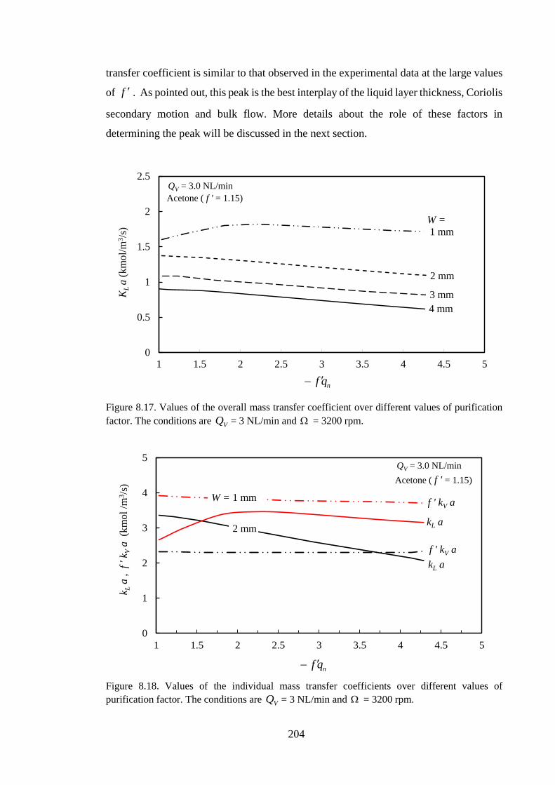
204
0
0.5
1
1.5
2
2.5
1 1.5 2 2.5 3 3.5 4 4.5 5
KL
a (
km
ol/
m3/s
)
4 mm
2 mm
W =
1 mm
QV = 3.0 NL/min
3 mm
Acetone ( f ' = 1.15)
nqf −
0
1
2
3
4
5
1 1.5 2 2.5 3 3.5 4 4.5 5
k La
,
f ' k V
a
(km
ol
/m3/s
)
2 mm
QV = 3.0 NL/min
Acetone ( f ' = 1.15)
W = 1 mm
nqf −
kL a
f ' kV a
kL a
f ' kV a
transfer coefficient is similar to that observed in the experimental data at the large values
of . As pointed out, this peak is the best interplay of the liquid layer thickness, Coriolis
secondary motion and bulk flow. More details about the role of these factors in
determining the peak will be discussed in the next section.
Figure 8.17. Values of the overall mass transfer coefficient over different values of purification
factor. The conditions are VQ = 3 NL/min and = 3200 rpm.
Figure 8.18. Values of the individual mass transfer coefficients over different values of
purification factor. The conditions are VQ = 3 NL/min and = 3200 rpm.
f

205
0 1 2 3 4 5 6 7
0
0.5
1
1.5
2
2.5
3
0 1 2 3 4 5 6 7 8 9 10
QV (NL/min)
KLa
, k L
a ,
f ' k V
a
(km
ol
/m3/s
)
QL (mL/min)
KLa
f ' kV a
kL a
-f 'qn= 1.2
Acetone ( f '= 1.15)
'qn
Different Gas and Liquid Flow Rates
The experiments and the computations carried out in this work are based on fixing
the flow rate of one of the phases, usually the gas phase, and change the other. However,
it is important to examine how varying these parameters together affects the process of
contacting. Fig. 8.19 below shows the sensitivity of the transfer coefficients to different
values of gas and liquid flow rates. Again, the purification factor ( nqf − ) and are
fixed at 1.2 and 1.15, respectively, for all the cases. Also, before discussing the results,
it is worth mentioning that the range of gas and liquid flow rates shown in Fig. 8.19
corresponds to a range of Reynolds number of 243Re −L and 2150270Re −V .
Figure 8.19. Mass transfer coefficients over different values of gas and liquid flow rates. The
other conditions are = 1.15 , nqf − = 1.2 and = 3200 rpm.
Considering the results of the gas phase first (red curve), the behaviour is
immediately evident: akf V increases gradually as the gas phase flow rate increases.
There is no doubt that this effect is mainly due to increasing Reynolds number (ratio of
convective effect to the viscous effect) which, in turn, results in a stronger Coriolis
motion, enhancing mass transfer by convection. On the other hand, the solute mass
transfer in the liquid side (blue curve) reveals an interesting behaviour. It can be seen
f
f

206
clearly that akL increases as the liquid flow rate increases (labels on the upper abscissa)
and then starts decreasing at around LQ > 4.5 mL/min, forming a wide peak. This
behaviour can be interpreted in terms of both the liquid layer thickness and the combined
effect of the main flow and secondary flow. It must be clear now that at a low liquid flow
rate, the interface shape imposes a situation where the diffusion length scale is large at
the ends compared to that at the middle of the layer (due to the menisci formation) and a
large fraction of the fluid is diverted there. Also, it must be known that small liquid flow
rate means a weak secondary flow generated in the menisci regions. So the rapid increase
in akL with the liquid flow rate (from 0.7 to about 3 mL/min) is mainly because the
menisci effect is minimised along with the expected increase in secondary motion with
the liquid flow rate. The variation in menisci effect with the liquid phase flow rate can
be seen clearly in Fig. 8.20 through the progression in solute mole fraction distribution.
As the liquid flow rate increases, the liquid layer increases and hence a large portion of
liquid flow rate is diverted in the middle of the layer, affecting directly the solute
concentration distribution.
The effect of streamwise convection in the liquid side is also clear in Fig. 8.20 (i.e.
dzdYw LBL perpendicular to the direction of diffusion, LBL YD ). Because Lw increases
with distance from the wall, a strong variation in solute distribution occurs across the
flowing liquid (i.e. colour changes from dark red to light red) and it increases with the
liquid flow. Diffusive transfer, in general, is proportional directly with the difference in
solute concentration. But increasing the liquid flow rate has an opposite effect as well.
It leads to increasing both the layer thickness and hence the diffusion length scale and the
axial mass transfer by the bulk flow. Thus, any dropping in mass transfer due to increasing
the diffusion distance and the bulk flow appears to be over-compensated by the increased
effect of secondary motions and the solute difference across the flowing fluid. This likely
explains the continuous increase in akL observed in Fig. 8.19, reaching an optimum at
LQ around 4.5 mL/min. Further increasing the liquid phase flow rate, however, the mass
transfer will be more affected by the decreasing effect of liquid layer thickness and the
axial mass transfer along the channel and hence akL decreases.
The overall mass transfer coefficient is a direct result of the variation in the individual
coefficients seen in Fig. 8.19, particularly akf V . Accordingly, aKL increases first as
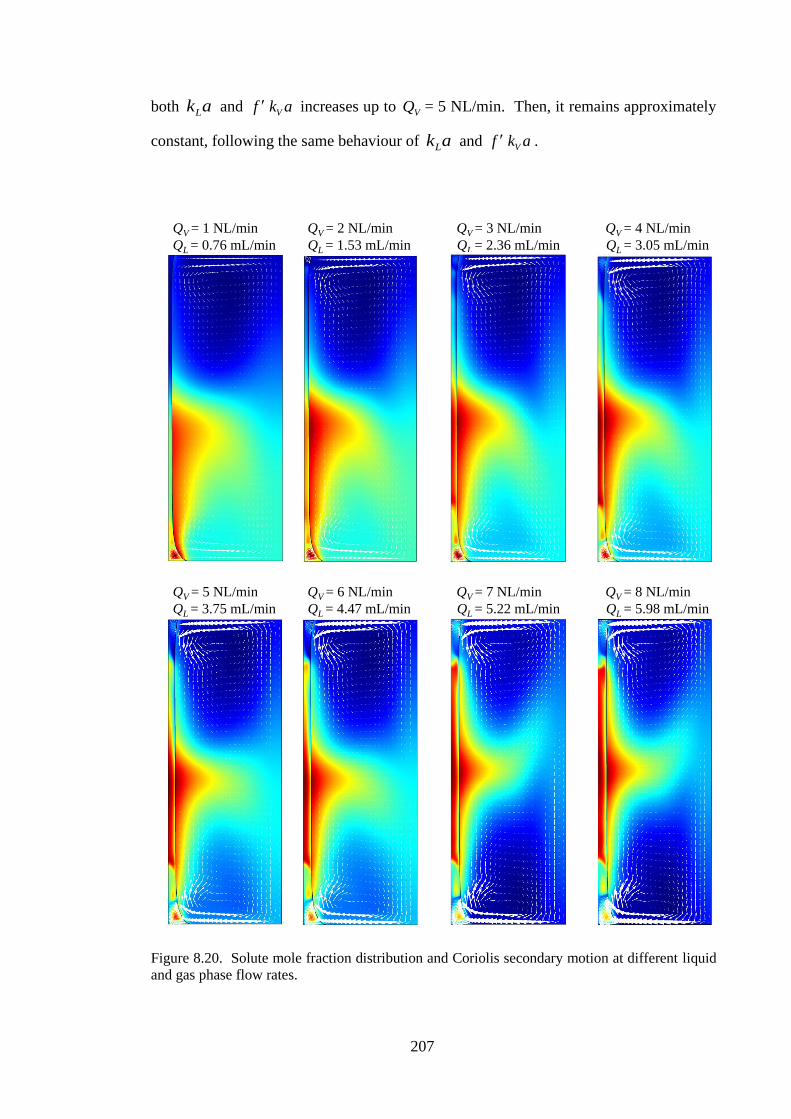
207
QV = 5 NL/min QV = 6 NL/min QV = 7 NL/min QV = 8 NL/min
QL = 3.75 mL/min QL = 4.47 mL/min QL = 5.22 mL/min QL = 5.98 mL/min
QV = 1 NL/min QV = 2 NL/min QV = 3 NL/min QV = 4 NL/min
QL = 0.76 mL/min QL = 1.53 mL/min QL = 2.36 mL/min QL = 3.05 mL/min
both akL and akf V increases up to VQ = 5 NL/min. Then, it remains approximately
constant, following the same behaviour of akL and akf V .
Figure 8.20. Solute mole fraction distribution and Coriolis secondary motion at different liquid
and gas phase flow rates.

208
8.4 Summary
Computational results for gas-liquid contacting in a rotating spiral channel have been
presented in this chapter. The first part of the chapter was dedicated to assessing the 2-D
computational approach adopted in this research. It was tested by predicting a range of
experimental data. The approach gives an excellent prediction of the liquid layer thickness
(MacInnes and Zambri, 2015) and a good prediction of mass transfer parameters ( and
aKL ) over a wide range of experimental conditions. However, it was less good at
conditions where the liquid flow rate is small (or large nqf − ) for the large values.
The model sensitivity analysis using an interface shape with a larger meniscus size
suggests that the difference is likely due to the approximations used in the interface shape
calculations.
In the second part of the chapter, a parametric analysis was conducted to demonstrate
the flexibility of rotating spiral contacting. In the analysis, the effect of three key
parameters (rotation rate, channel aspect ratio and phase flow rates) on desorption of
acetone was studied. Interestingly, the results showed that some of these parameters can
be adjusted and others can be engineered to enhance the contacting process. First, by
adjusting the rotation rate, the contacting process can be optimised. For a range between
1000-20,000 rpm, it was found that =16,000 rpm gives a maximum mass transfer
coefficient. Second, by changing the channel aspect ratio, the contacting process can be
enhanced considerably. It was found that reducing the width from 4 mm to 1 mm
increases the mass transfer coefficient approximately by a factor of two. Finally, at a
given rotation rate and channel aspect ratio, the mass transfer can be enhanced by
adjusting the flow rate of the contacting phases. It was found that increasing the flow rate
of both phases increases the mass transfer coefficient also by about a factor of two.
Ld
f
209
Chapter Nine
9 General Conclusions and Future Trends
The rotating spiral technique is an emerging separation approach with the potential
to handle any two immiscible fluid phases. In this work, experimental and 2-D numerical
investigations of physical mass transfer in a rotating spiral channel were conducted over
a wide range of phase and solute systems. The main aim was to understand and
demonstrate the performance of this technique for gas-liquid contacting. The work began
by establishing a theoretical framework based on a bulk analysis of counter-current
contacting (Chapter 3). This enabled experimental analysis and a comparison between
approaches under different contacting conditions. The term ‘total specific throughput ‘,
which is the ratio of treated phase throughput to the contactor volume, was presented as
the comparison criterion in this research. A 2-D computational model was detailed in
Chapter 4 and a series of computations were conducted. The purpose of these
computations was: (1) to understand the general character of the flow and the process of
solute transfer at different gas and liquid phase flow rates and (2) to benchmark the
numerical solution by predicting results for the wide-channel model, which has an
analytical solution. Experimentally, desorption of four different dilute solutes from water
into air were studied separately over a range of contacting conditions. The procedures to
conduct the experiments and to take measurements were presented in Chapter 5. The list
of physical properties used throughout this work were given in Chapter 6. The
experimental findings and a comparison of the rotating spiral approach to other alternative
approaches were discussed in Chapter 7. In Chapter 8, the predictions of the 2-D
computational model were assessed and a parametric study was carried out to highlight
the role of rotation rate, the channel aspect ratio and the effect of phase flow rates.
The main findings and conclusions of this research are presented in this chapter. This
is followed by recommendations, suggesting research directions for further future work.
It is helpful to note here that a detailed conclusion for each portion of this work were
covered at the end of each chapter.
210
Conclusions
General Characteristics
The computations carried out in Chapter 4 revealed important characteristics of gas-liquid
contacting in a spiral channel with a relatively large aspect ratio. The results indicated
that there was strong Coriolis secondary motion in the gas phase, while in the liquid phase
there were just two weak vortices active only in the meniscus regions. This secondary
motion, in the gas-phase, has a strong distortional effect on the gas streamwise velocity.
The distortion observed in the gas-phase and the structure of the Coriolis motion were
consistent with the experimental findings and computations reported in the literature for
a single fluid flow in a rotating channel. So there was a strong reason to believe that the
essential features of the flow were captured by the 2-D computations. The main flow and
the secondary flow determined the solute concentration distribution in the spiral, and
hence, the mass transfer performance. The numerical results at = 3200 rpm given in
Chapter 4 clearly demonstrated that increasing the gas phase flow rate produced stronger
Coriolis motion, thereby improving the mass transfer of the gas side, with little impact on
the liquid layer thickness. In the liquid phase, on the other hand, it was found that
increasing the liquid phase flow rate increased the liquid layer thickness and changed the
structure of Coriolis secondary motion. The motion became vigorously active in the
corners and produced small roll-cells, stretching towards the central part of the liquid
layer. This evolved motion also enhanced the mass transfer in the liquid side through
convection. Interestingly, the comparison between the model results (with and without
Coriolis terms) and the mass transfer measurements made in Chapter 8 showed that the
mass transfer could be doubled due to the effect of secondary motions in both the gas and
liquid phases.
Rotating Spiral Performance
A wide range of experiments were performed to establish the performance of a
rotating spiral channel by studying individually desorption of ethanol, acetonitrile,
acetone and MEK from water using air as a stripping agent. The spiral temperature, gas
phase flow rate and liquid phase flow rate were varied while the rotation rate and pressure
were maintained at 3200 rpm and 1.8 bara, respectively. The experimental results were
given in Chapter 7 and showed the capability of the spiral to handle this variety of
systems, achieving approximately solute-free water when the appropriate flow rate ratio

211
was selected. Such simplification greatly reduces manufacturing and device design costs,
in addition to providing an inherently flexible piece of equipment.
Also, one of the more significant findings emerged from the experiments was that
there was a universal peak in the mass transfer coefficient at a liquid layer thickness
between 80-90 µm. This occurred independently of the gas phase flow rate and
prominently appeared in the data for the systems with large (3.38 and 5.5) where mass
transfer was greatly affected by the liquid phase. At a small liquid phase flow rate, most
of the liquid was shifted into the corners (menisci regions) where mass transfer was poor,
a large diffusion path accompanied weak Coriolis motion. By increasing the liquid flow
rate, the effect of menisci decreased with a stronger Coriolis motion, leading to an
increased mass transfer coefficient, up until the peak value. Any further increasing of the
liquid phase flow rate, however, resulted in the liquid layer thickness and the axial mass
transfer along the channel increasing, and hence decreased. The effect of menisci
on the flow, and hence mass transfer, and the mechanism of peak determination is
confirmed by the 2-D computational results given in Chapter 8.
Significantly, this finding strengthens the idea that the spiral can identify successfully
the optimum contacting and this optimum prevails along the contacting channel. At a
given rotation rate, the spinning of spiral produces a constant longitudinal body force
which drives mainly the liquid phase along the channel and a transverse body force which
keeps the phases separated. So the phases do not mix and hence the gas phase does not
affect strongly the liquid layer thickness. Therefore, as in the experiments, by changing
only the liquid phase flow rate, which in turn changes the liquid layer thickness, the peak
in can be identified. Since this peak is weakly dependent on the gas phase flow rate,
it can be tailored to the desired nqf − by changing only the gas phase flow rate. In
principle, therefore, it seems that optimum contacting, represented by , and optimum
usage of solvent, determined by nqf − , can be achieved simultaneously by using the
rotating spiral technique.
f
aKL
aKL
aKL

212
Relative Performance
Before this study, evidence regarding spiral channel performance relative to other
approaches was purely anecdotal. The rotating spiral can be thought of as a new
contacting approach and it is important to be placed into the context of other alternative
contacting methods. For this purpose, a total specific throughput based on molar flow
rate was used to enable a fair comparison between results of absorption and desorption
taken from different contactors and those collected by the current spiral. This comparison
measure is linked inversely to the contactor size and contacting time scale. So a higher
specific throughput means a smaller contactor size can be used to achieve a given
throughput at a given purification. The comparison results were shown in Chapter 7 and
indicated that the spiral channel allowed total specific throughput to be many times larger
than that for the other methods. Comparison with dispersed-phase contactors data
(packed column and rotating packed bed) showed that total specific throughput of the
spiral was about three times larger in the expected region of operation which is around
1 < nqf − < 4. For parallel-flow contactors, recent data of desorption of acetone using a
membrane microchannel (Adiche, 2018) were considered in the comparison.
Interestingly, the phase and solute system as well as the contacting conditions in this study
were, approximately, the same as those tested in the spiral. However, the results also
indicated that the spiral could produce a larger specific throughput by factor of two in
relation to this contactor in the appropriate range of nqf − . This difference is, perhaps,
due to the convective effect of the Coriolis motion in the spiral and the additional mass
transfer resistance added by the membrane which together may lead to such difference.
Prediction of the 2-D Computational Model
The study adopted a computational model based on solving the governing equations
in a 2-D section using an interface shape predicted independently. In this work, this
computational model was assessed using a range of experimental data and the results were
presented in Chapter 8. A comparison with the experimental data of MacInnes and
Zambri (2015) showed that this model could reliably capture the liquid layer thickness
over a range of liquid phase flow rates for three different rotation rates (1480, 2400 and
3840 rpm). In terms of the mass transfer, the 2-D model predicted the experimental mass
transfer coefficient over most of the range of data but it also failed in some instances. In
particular, the 2-D model over-predicted aKL values at a low liquid phase flow rate (or

213
large nqf − ) for the systems with large (3.38 and 5.5). The model sensitivity analysis
using an interface shape with a larger meniscus size suggested that the difference is likely
due to the approximations used in the interface shape calculations. One of these
approximations is using contact angles measured at static conditions. In practice, these
angles might be more sensitive to other processes, such as evaporation, during the
contacting process. Any changes in the contact angles affect the meniscus size, which is
a crucial parameter in determining the mass transfer at low liquid phase flow rates.
However, without adjusting the contact angles and using a local radial position ( 0R = 25
mm) and water surface tension (0.07 N/m), the 2-D model predicts convincingly the data
especially over nqf − values between 1 and 4 which are a typical for desorption process.
Model Parametric Study
The final piece of this research was a parametric study using the 2-D model to
investigate the effect of three key parameters: rotation rate, channel aspect ratio and both
the gas and liquid phase flow rate. The effect of these parameters has not been
studied experimentally and it is important to understand their role in gas-liquid
contacting process. For this objective, desorption of acetone ( = 1.15) at nqf − = 1.2
and = 3200 rpm was taken a reference case to carry out the study.
Interestingly, the 2-D numerical results showed that the channel geometry can be
engineered and the rotation rate and phase flow rates can be adjusted to enhance the
rotating spiral contacting. It was found that reducing the channel width from 4 mm to 1
mm increased the mass transfer coefficient approximately by a factor of two. This
reduction in channel width changed the strength of Coriolis motion in both phases. It
became stronger and occupied most the gas and liquid phase passage, resulting in
improving the mass transfer. Further, the rotation rate, which is a key operating
parameter, was examined over a range between 1000-20,000 rpm. The results showed
that by adjusting the rotation rate, the contacting process could be optimised. By
increasing the rotation rate, three main changes occurred: (1) the shape of the interface
flattened, (2) the liquid layer thickness decreased and (3) the Coriolis motion in the gas
phase increased. These three changes improved the mass transfer of acetone in both
phases achieving a maximum mass transfer coefficient at around =16,000 rpm. The
other parameter examined was the flow rate of the contacting phases. The flow rate of the
f
f

214
gas phase and the liquid phase can be controlled simultaneously at a desired nqf − during
operation. In practice, this can be done by simply adjusting a needle valve or pump
setting. The 2-D model results showed that increasing the flow rate of both phases from
VQ =1 NL/min and LQ = 0.76 mL/min to VQ = 8 NL/min and LQ = 5.98 mL/min
increases the mass transfer coefficient by about a factor of two. This was mainly
attributed to the convective effect of Coriolis motion in the gas and liquid phase. This
study provides evidence that the 2-D modelling approach established here can be a useful
tool for the improvement of the rotating spiral technique.
Future Trends
In this section, some recommendations for further development and investigation are
suggested to build upon the current research systematically.
Experimental Work
9.2.1.1 Turbulent Flow Regime
The experiments in this work were restricted to laminar flow in order to ensure a
stable flow in each phase. However, it may be possible to investigate the performance of
the spiral at higher Reynolds number or possibly even reaching the turbulent flow regime
in one of the phases. One of the most challenges of such study is to determine the
Reynolds number limits that can be achieved practically in the two phases such that a
stable flow can be obtained. Using the wide-channel model (Chapter 4) and conservative
values of the Froude number ( Fr = 0.5) and Weber number ( We = 5) defined in Chapter
2, one can quantify roughly the maximum allowable limits of Reynolds number. The
results over the broadest possible range of phase and solute systems ( ) and the required
range of rotation rates are shown in Fig. 9.1 and Fig. 9.2, respectively. The spiral
geometrical parameters used in the calculations are 0R = 25 mm (minimum radius of the
spiral), t = 3 mm (spacing between the channels) and different heights ( h ). Fig. 9.1
clearly indicates that it is possible to achieve high Reynolds number (reaching turbulent
flow) in the gas phase for systems with > 1 (Fig. 9.1). Equally, the results in Fig. 9.2
shows that the smaller channel, which provides a higher surface area per unit volume,
requires larger rotation rate. Moving from a 7 mm channel height down to a 1 mm height
at = 1, for example, increases the rotation rate by a factor of 75. Considering the
f
f
f
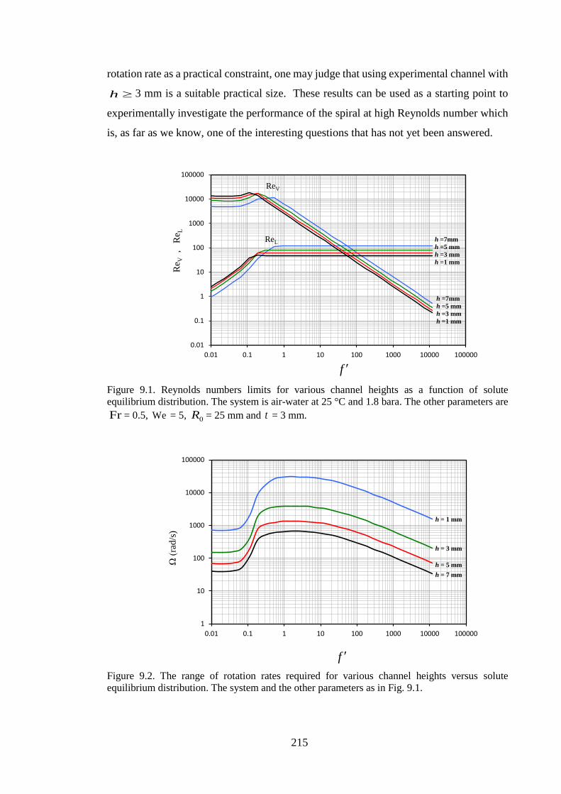
215
1
10
100
1000
10000
100000
0.01 0.1 1 10 100 1000 10000 100000
Ω (
rad/s
)
h = 1 mm
h = 3 mm
h = 5 mm
h = 7 mm
f
0.01
0.1
1
10
100
1000
10000
100000
0.01 0.1 1 10 100 1000 10000 100000
Re V
,
R
e L
ReV
ReL h =7mm
h =5 mm
h =3 mm
h =1 mm
h =7mm
h =5 mm
h =3 mm
h =1 mm
f
rotation rate as a practical constraint, one may judge that using experimental channel with
h 3 mm is a suitable practical size. These results can be used as a starting point to
experimentally investigate the performance of the spiral at high Reynolds number which
is, as far as we know, one of the interesting questions that has not yet been answered.
Figure 9.1. Reynolds numbers limits for various channel heights as a function of solute
equilibrium distribution. The system is air-water at 25 °C and 1.8 bara. The other parameters are
Fr = 0.5, We = 5, 0R = 25 mm and t = 3 mm.
Figure 9.2. The range of rotation rates required for various channel heights versus solute
equilibrium distribution. The system and the other parameters as in Fig. 9.1.

216
9.2.1.2 Other Applications
The process of gas-liquid contacting in a rotating spiral channel was demonstrated
here. However, there are other applications within the capability of this approach that
have not been investigated. Liquid-liquid extraction, perhaps, is the most attractive
research area. The spiral can handle liquids with different viscosities and densities and
that is key to effective liquid-liquid contacting. Using the same experimental and
theoretical approach of the current study, many questions can be answered concerning
liquid-liquid contacting such as the role of Coriolis force, phase Reynolds number and
rotation rate. Furthermore, the present research showed the flexibility of spiral channel
to produce a wide range of mass transfer measurements and these measurements can be
predicted precisely over a range of conditions. This distinctive feature of the spiral can
be employed in many analytical applications such as physical properties determination.
In general, there is a lack of information about solute diffusion coefficients, particularly
in the liquid phase, and solute equilibrium distribution. With the spiral technique, this
necessary information can be determined rapidly and accurately for a given phase and
solute system using the 2-D model in parallel with a few number of experiments.
However, this inversion estimation method needs to be developed and tested over the
largest conceivable range of solute properties and this is another research trend that can
be further investigated.
Further Modelling Work
The 2-D model presented in the work was about a mass transfer process between two
immiscible phases contacting in a section of rotating spiral channel. A case of dilute solute
was considered and no other physical processes were included. However, this level of
modelling can be extended by taking into account other effects such as heat transfer and
chemical reaction. Processes such as distillation or chemical separation certainly require
a more comprehensive model to be investigated thoroughly using the same 2-D analysis
made in this work. Further, the 2-D approximations proposed in this research were based
on replacing the solute concentration change at any location in the section ( zY ) by
the local bulk gradient ( dzdYB ). For fast chemical reactions or the presence of a high
concentration solute, the change in solute concentration along the channel may not occur
in a gradual manner and hence this approximation may no longer be justified. So in this
case, ideally, one would like to quantify the effect of this approximation. This requires

217
12 cm
18 cm 1.8 m
1.5 m
Units in arrays to
handle larger
throughput
25-channel stack
50-unit array
developing a numerical solution for the governing equations in a 3-D spiral segment,
which is expected to be computationally expensive.
Further, studying the process of contacting in a turbulent regime (as suggested in
Section 9.2.1) requires developing a turbulence model to deepen understanding of this
complex process. This is another research direction that can be taken on board. It is
expected that such a theoretical investigation along with the experiments suggested in the
previous section will be a tremendous step to advance this novel technology.
Technology Developments
Further work to develop the spiral technology can be made. It is important to
recognise that the flow rate of the gas phase and the liquid phase were small in the
experimental channel. The maximum gas phase flow rate tested here, for example, was
6.2 NL/min which is equivalent to about 20 kg/day/channel. The idea of stacking multiple
spiral channels is raised in MacInnes and Zambri (2015) since this increases the actual
throughput. Scaling-out the contacting unit by stacking 25 channels identical to the one
used in the experiments would result in a throughput of 500 kg/day/unit. The conceptual
design of the unit and its dimensions are shown in Fig. 9.3. It is believed that such a flow
rate would meet the production requirements of many small chemical industries.
Achieving larger throughput could be conceived by using an array of units connected
together. Of course, such development would not be straightforward and a research effort
would need to be devoted to that direction in the future.
Figure 9.3. Conceptual design of a separation unit consisting of a multiple spiral channels.

218
References
Abdulrazzaq, N., Al‐Sabbagh, B., Rees, J.M. and Zimmerman, W.B., 2016. Separation of
azeotropic mixtures using air microbubbles generated by fluidic oscillation. AIChE
Journal, 62(4), pp.1192-1199.
Abrams, D.S. and Prausnitz, J.M., 1975. Statistical thermodynamics of liquid mixtures: a new
expression for the excess Gibbs energy of partly or completely miscible systems. AIChE
Journal, 21(1), pp.116-128.
Adiche, C., 2018. Stripping of acetone from water in a microchannel device. Separation and
Purification Technology, 199, pp. 105–113.
Al-Rawashdeh, M., Cantu-Perez, A., Ziegenbalg, D., Löb, P., Gavriilidis, A., Hessel, V. and
Schönfeld, F., 2012. Microstructure-based intensification of a falling film microreactor through
optimal film setting with realistic profiles and in-channel induced mixing. Chemical Engineering
Journal, 179, pp. 318–329.
Al-Rawashdeh, M., Hessel, V., Lob, P., Mevissen, K., Schonfeld, F., 2008. Pseudo 3-D
simulation of a falling film microreactor based on realistic channel and film profiles. Chemical
Engineering Science, 63(21), pp.5149–5159.
Al-yaqoobi, A., Hogg, D. and Zimmerman, W. B., 2016. Microbubble Distillation for Ethanol-
Water Separation. International Journal of Chemical Engineering, 2016, pp. 1–10.
Anderson, T. F. and Prausnitz, J. M., 1978. Application of the UNIQUAC Equation to Calculation
of Multicomponent Phase Equilibria. 1. Vapor-Liquid Equilibria. Ind. Eng. Chem. Process Des.
Dev., 17(4), pp. 552–561.
Anvaripour, B., Yoswathana, N., Ashtoif, N. and Arrowsmith, A., 1995. Stripping ethanol and
acetone from water with modern packings. Transactions on Ecology and the Environment, 7, pp.
493–500.
Aota, A., Mawatari, K. and Kitamori, T., 2009. Parallel multiphase microflows: fundamental
physics, stabilization methods and applications. Lab on a chip, 9(17), pp. 2470–2476.
Arnold, J. H., 1930. Studies in diffusion. I.–Estimation of diffusivities in gaseous systems.
Industrial and Engineering Chemistry, 22(10), pp. 1091–1095.
219
Atik, Z., Gruber, D., Krummen, M. and Gmehling, J., 2004. Measurement of Activity Coefficients
at Infinite Dilution of Benzene, Toluene, Ethanol, Esters, Ketones, and Ethers at Various
Temperatures in Water Using the Dilutor Technique. J. Chem. Eng. Data, 49(5), pp. 1429–1432.
Ayash, A. A. and MacInnes, J. M., 2017. Mass Transfer Prediction of Gas-Liquid Contacting in
a Rotating Spiral Channel. in the 4th International Conference of Fluid Flow, Heat and Mass
Transfer (FFHMT’17). Toronto, Canada, pp. 1–8.
Barua, S. N., 1954. Secondary flow in a rotating straight pipe. Proc. R. Soc. Lond. A 227, pp.
133–139.
Bašić, A. and Duduković, M.P., 1995. Liquid holdup in rotating packed beds: examination of the
film flow assumption. AIChE Journal, 41(2), pp.301–316.
Batchelor, G.K., 2000. An introduction to fluid dynamics. Cambridge University Press.
Beak, J. H. and Ko, C. H., 2000. Numerical Flow Analysis in a Rotating Square Duct and a
Rotating Curved-Duct. International Journal of Rotating Machinery, 6(1), pp. 1–9.
Benton, G. S., 1956. The Effect of the Earth’s Rotation on Laminar Flow in Pipes. J. Appl. Mech,
23, pp. 123–127.
Bergmann, D. L. and Eckert, C. A., 1991. Measurement of limiting activity coefficients for
aqueous systems by differential ebulliometry. Fluid Phase Equilibria, 63(1-2), pp. 141–150.
Bird, R.B., Stewart, W.E., and Lightfoot, E. N., 2007. Transport Phenomena. 2nd edn. John Wiley
& Sons,Inc.
Boomkamp, P. A. M. and Miesen, R. H. M., 1996. Classification of instabilities in parallel two-
phase flow. International Journal of Multiphase Flow, 22(1967), pp. 67–88.
Brandani, S., Brandani, V., Del Re, G. and Di Giacomo, G., 1991. Activity coefficients from a
virial expansion about their infinite-dilution values. The Chemical Engineering Journal, 46(1),
pp.35–42.
Bredwell, M.D. and Worden, R.M., 1998. Mass‐transfer properties of microbubbles. 1.
Experimental studies. Biotechnology Progress, 14(1), pp.31–38.
Burns, J.R. and Ramshaw, C., 1996. Process intensification: visual study of liquid maldistribution
in rotating packed beds. Chemical Engineering Science, 8(51), pp.1347–1352.

220
Charpentier, J. C., Chimiques, I. and France, N., 1976. Review Paper Recent Progress in Two
Phase Gas-Liquid Mass Transfer in Packed Beds. Chemical Engineering Journal, 11(3), pp. 161–
181.
Chasanis, P., Kehrmann, K. M., Kern, J., Zecirovic, R., Grünewald, M. and Kenig, E. Y., 2011.
Investigation of a microstructured high efficiency contactor. Chemical Engineering and
Processing: Process Intensification, 50(11–12), pp. 1244–1251.
Chen, Y.S., Lin, C.C. and Liu, H.S., 2005. Mass transfer in a rotating packed bed with various
radii of the bed. Industrial & engineering chemistry research, 44(20), pp.7868–7875.
Chen, Y.S. and Liu, H.S., 2002. Absorption of VOCs in a rotating packed bed. Industrial &
engineering chemistry research, 41(6), pp.1583–1588
Chiang, C. Y., Chen, Y. S., Liang, M. S., Lin, F. Y., Tai, C. Y. Der and Liu, H. S., 2009.
Absorption of ethanol into water and glycerol/water solution in a rotating packed bed. Journal of
the Taiwan Institute of Chemical Engineers, 40(4), pp. 418–423.
COMSOL, A., 2008. COMSOL multiphysics version 3.5, User’s guide and reference guide. from:
http://math. nju. edu.cn/help/mathhpc/doc/comsol/command. pdf. [Accessed 30/01/2015].
Comyn, J., Mascia, L., Xiao, G. and Parker, B.M., 1996. Plasma-treatment of polyetheretherketone
(PEEK) for adhesive bonding. International Journal of Adhesion and Adhesives, 16(2), pp.97–104.
Constantinou, A., Barrass, S., Pronk, F., Bril, T., Wenn, D. A., Shaw, J. E. A. and Gavriilidis, A.,
2012. CO2 absorption in a high efficiency silicon nitride mesh contactor. Chemical Engineering
Journal , 207–208, pp. 766–771.
Constantinou, A. and Gavriilidis, A., 2010. CO2 absorption in a microstructured mesh reactor.
Ind. Eng. Chem. Res., 49(3), pp. 1041–1049.
Constantinou, A., Ghiotto, F., Lam, K.F. and Gavriilidis, A., 2014. Stripping of acetone from
water with microfabricated and membrane gas–liquid contactors. Analyst, 139(1), pp.266-272.
Coulson, J. M., Rcharson, J. F., Backhurst, J. R. and Harker, J. H., 2002. Particle Technology and
Separation Processes. 5th edn. Bath, UK: The Bath Press.
Cussler, E. L., 1997. Diffusion: Mass Transfer in Fluid Systems. 3rd edn. UK: Cambridge
University Press.

221
Cypes, S. H. and Engstrom, J. R., 2004. Analysis of a toluene stripping process: A comparison
between a microfabricated stripping column and a conventional packed tower. Chemical
Engineering Journal, 101(1–3), pp. 49–56.
Eckert, J. S., 1970. Trays and packings: selecting Proper Distillation Column Packing. Chemical
Engineering Progress, 66(3), p. 39–44.
Edmister, W. C., 1957. Absorption and stripping‐factor functions for distillation calculation by
manual‐and digital‐computer methods. AIChE Journal, 3(2), pp. 165–171.
French, H. T., 1987. Vapour pressures and activity coefficients of (acetonitrile + water) at 308.15
K. The Journal of Chemical Thermodynamics, 19(11), pp. 1155–1161.
Fuller, E.N., Ensley, K. and Giddings, J.C., 1969. Diffusion of halogenated hydrocarbons in
helium. The effect of structure on collision cross sections. The Journal of Physical
Chemistry, 73(11), pp.3679–3685.
Gabelman, A. and Hwang, S.T., 1999. Hollow fiber membrane contactors. Journal of Membrane
Science, 159(1-2), pp.61–106.
Geankoplis, C. J., 2003. Transport Processes and Unit Operations. 3rd edn. London: Prentice-
Hall international (UK) Limited.
Gibbon, H.J., Wainwright, J. and Rogers, R.L., 1994. Experimental determination of flammability
limits of solvents at elevated temperatures and pressures. In Institution of Chemical Engineers
Symposium Series (Vol. 134, pp. 1-1). HEMSPHERE PUBLISHING CORPORATION.
Gierczak, T., Burkholder, J. B., Bauerle, S. and Ravishankara, A. R., 1998. Photochemistry of
acetone under tropospheric conditions. Chemical Physics, 231, pp. 229–244.
Górak, A. and Stankiewicz, A., 2011. Intensified reaction and separation systems. Annual review
of chemical and biomolecular engineering, 2, pp.431–451.
Gregersen, M. M., Okkels, F., Bazant, M. Z. and Bruus, H., 2009. Topology and shape
optimization of induced-charge electro-osmotic micropumps. New Journal of Physics, 11(7), pp.
1–21.
Habibullah, M., Rahman, I. M. M., Uddin, M. A., Iwakabe, K., Azam, A. and Hasegawa, H.,
2011. Densities and Viscosities of the Binary Mixtures of Phenylmethanol with 2-Butanone’,
Journal of Chemical and Engineering Data, 56(8), pp. 3323–3327.

222
Haidl, J., Rejl, F. J., Valenz, L., Kordač, M., Moucha, T., Labík, L. and Schultes, M., 2016.
Absorption in wetted-wall column with phase properties close to distillation conditions. Chemical
Engineering Science, 144, pp. 126–134.
Harries, D., Holler, J. F. and Crouch, S. R., 2007. Principles of Instrumental Analysis. 6th edn.
Canada: Thomson Brooks/Cole.
Hart, J. E., 1971. Instability and Secondary Motion in a Rotating Channel Flow. J Fluid Mech,
45(2), pp. 341–351.
Hartwick, R. P. and Howat, C. S., 1995. Infinite Dilution Activity Coefficients of Acetone in
Water. A New Experimental Method and Verification. J. Chem. Eng. Data, 40(4), pp. 738–745.
Hayduk, W. and Laudie, H., 1974. Prediction of diffusion coefficients for nonelectrolytes in dilute
aqueous solutions. AIChE Journal, 20(3), pp.611–615.
Hessel, V., Angeli, P., Gavriilidis, A. and Löwe, H., 2005. Gas-liquid and gas-liquid-solid
microstructured reactors: Contacting principles and applications. Industrial and Engineering
Chemistry Research, 44(25), pp. 9750–9769.
Ho-Le, K., 1988. Finite element mesh generation methods: a review and classification. Computer-
Aided Design, 20(1), pp. 27–38.
Houston, R. and Walker, C., 1950. Absorption in Packed Towers. Effect of Molecular Diffusing
on Gas Film Coefficient. Industrial & Engineering Chemistry, 42(6), pp. 1105–1112.
Hovorkaa, Š., Dohnala, V., Rouxb, A. H. and Roux-Desgranges, G., 2002. Determination of
temperature dependence of limiting activity coefficients for a group of moderately hydrophobic
organic solutes in water. Fluid Phase Equilibria ·, 201(1), pp. 135–164.
Howard, K.S. and McAllister, R.A., 1957. Surface tension of acetone‐water solutions up to their
normal boiling points. AIChE Journal, 3(3), pp.325-329.
Howard, K. S. and McAllister, R. A., 1958. The viscosity of acetone‐water solutions up to their
normal boiling points. AIChE Journal, 4(3), pp. 362–366.
Hsu, L. J. and Lin, C. C., 2012. Binary VOCs absorption in a rotating packed bed with blade
packings. Journal of Environmental Management, 98(1), pp. 175–182.
Huffman, J. R. and Urey, H. C., 1937. Separation of Oxygen Isotopes by a Fractionating Column.
Indutrial and Engineering Chemistry, 29(5), pp. 531–535.

223
Hwang, Y. L., Keller, G. E. and Olson, J. D., 1992. Steam Stripping for Removal of Organic
Pollutants from Water. 1. Stripping Effectiveness and Stripper Design. Industrial and
Engineering Chemistry Research, 31(7), pp. 1753–1759.
Ikehata, J., Shinomiya, K., Kobayashi, K., Ohshima, H., Kitanaka, S. and Ito, Y., 2004. Effect of
Coriolis force on counter-current chromatographic separation by centrifugal partition
chromatography. Journal of Chromatography A, 1025(2), pp. 169–175.
Iwakabe, K. and Kosuge, H., 2002. Determination and prediction of the isobaric vapor-liquid-
liquid equilibrium data. in the Proceedings of the International Conference on Distillation and
Absorption. Baden-Baden, Germany.
Javed, K. H., Mahmud, T. and Purba, E., 2006. Enhancement of mass transfer in a spray tower
using swiriling gas flow. Chemical Engineering Research and Design, 84(6), pp. 465–477.
Javed, K. H., Mahmud, T. and Purba, E., 2010. The CO2 capture performance of a high-intensity
vortex spray scrubber. Chemical Engineering Journal, 162(2), pp. 448–456.
Joel, A. S., Wang, M., Ramshaw, C. and Oko, E., 2017. Modelling, simulation and analysis of
intensified regenerator for solvent based carbon capture using rotating packed bed technology.
Applied Energy, 203, pp. 11–25.
Kadoya, .K, Matsunaga, N. and Nagashima, A., 1985. Viscosity and Thermal Conductivity of
Dry Air in the Gaseous Phase. J. Phys. Chem. Ref. Data, 14(4), pp. 947–970.
Khattab, I. S., Bandarkar, F., Fakhree, M. A. A. and Jouyban, A., 2012. Density, viscosity, and
surface tension of water+ethanol mixtures from 293 to 323K. Korean Journal of Chemical
Engineering, 29(6), pp. 812–817.
Kheshgi, H. S. and Scriven, L. E., 1985. Viscous flow through a rotating square channel. Physics
of Fluids, 28(10), pp. 2968–2979.
Kister, H.Z., Haas, J.R., Hart, D.R. and Gill, D.R., 1992. Distillation design (Vol. 1). New York:
McGraw-Hill.
Kohl, A. and Nielsen, R., 1997. Gas Purification. 5th edn. USA: Gulf Publishing Company.
Kojima, K., Zhang, S. and Hiaki, T., 1997. Measuring methods of infinite dilution activity
coefficients and a database for systems including water. Fluid Phase Equilibria, 131, pp. 145–
179.

224
Kowalczuk, P. B. and Drzymala, J., 2016. Some remarks on attachment of a gas bubble to another
phase both immersed in water. Physicochemical Problems of Mineral Processing, 52(1), pp.
147–154.
Kumar, M. P. and Rao, D. P., 1990. Studies on a High-Gravity Gas-Liquid Contactor. Industrial
& engineering chemistry research, 29(5), pp. 917–920.
Kunz, R. G. and Baade, W. F., 2001. Vapor-liquid activity coefficients for methanol and ethanol
from heat of solution data: application to steam-methane reforming. Journal of hazardous
materials, 88(1), pp. 53–62.
Kuvshinov, D., Bown, M. R., MacInnes, J. M., Allen, R. W. K., Ge, R., Aldous, L., Hardacre, C.,
Doy, N., Newton, M. I. and Mchale, G., 2011. Thermal conductivity measurement of liquids in a
microfluidic device. Microfluidics and Nanofluidics, 10(1), pp. 123–132.
Kwon, K.C., Ibrahim, T.H., Park, Y. and Simmons, C.M., 2004. Pseudo-binary molecular
diffusion of vapors into air. Advances in Environmental Research, 8(3-4), pp.667–678.
Lam, K. F., Sorensen, E. and Gavriilidis, A., 2013. Review on gas–liquid separations in
microchannel devices. Chemical Engineering Research and Design. Institution of Chemical
Engineers, 91(10), pp. 1941–1953.
Lamarre, B. and Shearouse, D., 1994. Air Stripping Industrial Wastewater. Pollution Engineering
:(United States), 26(9).
Langrish, T., Makarytchev, S., Fletcher, D. and Prince, R., 2003. Progress in Understanding the
Physical Processes Inside Spinning Cone Columns. Chemical Engineering Research and Design,
81(1), pp. 122–130.
Lee, G. H. and Baek, J. H. , 2002. A numerical study of the similarity of fully developed turbulent
flows in orthogonally rotating square ducts and stationary curved square ducts. International
Journal of Numerical Methods for Heat & Fluid Flow, 12(3), pp. 241–257.
Lee, G. H. and Baek, J. H., 2006. Effect of aspect ratio on the similarity between developing
laminar flows in orthogonally rotating ducts and stationary curved ducts. International Journal
of Numerical Methods for Heat & Fluid Flow, 16(4), pp. 494–508.
Lee G.H., Beak, J. H. , 2001. A numerical study on the similarity of laminar flows in orthogonally
rotating rectangular ducts and stationary curved rectangular ducts of arbitrary aspect ratio. in 7th
International Conference on Fluid Dynamics and Propulsion. Egypt, pp. 1–6.

225
Leva, M., 1954. Flow Through Irrigated Dumped Packings-Pressure drop, Loading, Flodding. In
Chem. Eng. Progr. Symp. Ser., 50(10), pp. 51–59.
Levenspiel, O., 1999. Chemical Recation Engineering. 3rd edn. New York: John Wiley & Sons,
Inc.
Li, Q., Ito, K., Wu, Z., Lowry, C. S. and Loheide, S. P., 2009. COMSOL multiphysics: A novel
approach to ground water modeling. Ground Water, 47(4), pp. 480–487.
Li, Y., Lu, Y., Liu, X. J., Wang, G., Nie, Y. and Ji, J., 2017. Mass-transfer characteristics in a
rotating zigzag bed as a Higee device’, Separation and Purification Technology. 186, pp. 156–
165.
Lin, C.C. and Chien, K.S., 2008. Mass-transfer performance of rotating packed beds equipped
with blade packings in VOCs absorption into water. Separation and Purification Technology,
63(1), pp. 138–144.
Lin, C. C., Wei, T. Y., Liu, W. T. and Shen, K. P., 2004. Removal of VOCs from gaseous streams
in a high-voidage rotating packed bed. Journal of Chemical Engineering of Japan, 37(12), pp.
1471–1477.
Liu, H., Lin, C., Wu, S. and Hsu, H., 1996. Characteristics of a rotating packed bed. Ind. Eng.
Chem. Res., 35(10), pp. 3590–3596.
Lobo, W. E., Friend, L., Hashmall, F. and Zenz, F., 1945. Limiting capacity of dumped tower
packings. Transactions of the American Institute of Chemical Engineers, 41(6), pp. 693–710.
Lockett, M. J., 1986. Distillation Tray Fundamentals. New York: Cambridge University Press.
Lugg, G. A., 1968. Diffusion coefficients of some organic and other vapors in air. Analytical
Chemistry, 40(7), pp. 1072–1077.
MacInnes, J. M., 2013. Prototype Channel Design Operation range for Rotating Spiral Phase
Contacting. (Personal communication, 26th April 2015).
MacInnes, J. M., Ayash, A. A. and Dowson, G. R. M., 2017. CO2 absorption using
diethanolamine-water solutions in a rotating spiral contactor. Chemical Engineering Journal, 307,
pp. 1084–1091.
226
MacInnes, J. M., Ortiz-Osorio, J., Jordan, P. J., Priestman, G. H. and Allen, R. W. K., 2010.
Experimental demonstration of rotating spiral microchannel distillation. Chemical Engineering
Journal, 159(1–3), pp. 159–169.
MacInnes, J. M., Pitt, M. J., Priestman, G. H. and Allen, R. W. K., 2012. Analysis of two-phase
contacting in a rotating spiral channel. Chemical Engineering Science, 69(1), pp. 304–315.
MacInnes, J. M., Priestman, G. H. and Allen, R. W. K., 2005. A Spinning Micro-Channel
Multiphase Contactor. in :7th World Congress of Chemical Engineering. Glasgow.
MacInnes, J. M. and Zambri, M. K. S., 2015. Hydrodynamic characteristics of a rotating spiral
fluid-phase contactor. Chemical Engineering Science, 126, pp. 427–439.
Mahmud, H., Kumar, A., Narbaitz, R. M. and Matsuura, T., 1998. Membrane air stripping : a
process for removal of organics from aqueous solutions. Separation Science and Technology,
33(14), pp. 2241–2255.
Makarytchev, S. V., Langrish, T. A. G. and Fletcher, D. F., 2005. CFD Analysis of Scale Effects
in Spinning Cone Columns. Chemical Engineering Research and Design, 83(8), pp. 951–958.
Makarytchev, S. V., Langrish, T. A. G. and Fletcher, D. F., 2002. CFD analysis of spinning cone
columns: Prediction of unsteady gas flow and pressure drop in a dry column. Chemical
Engineering Journal, 87(3), pp. 301–311.
Makarytchev, S. V, Langrish, T. A. G. and Fletcher, D. F., 2004. Mass transfer analysis of
spinning cone columns using CFD. Chemical Engineering Research and Design, 82(6), pp. 752–
761.
McCabe, W. L., Smith, J. C. and Harriott, P., 1993. Unit Operations of Chemical Engineering.
5th edn. New York: McGraw-Hill.
Mhiri, N., Monnier, H. and Falk, L., 2011. Intensification of the G/L absorption in microstructured
falling film application to the treatment of chlorinated VOC’s. Part III: Influence of gas thickness
channel on mass transfer. Chemical Engineering Science, 66(23), pp. 5989–6001.
Mochalova, N.S., Kholpanov, L.P. and Shkadov, V.Y., 1973. Hydrodynamics and mass transfer
in a liquid layer at a rotating surface. Journal of Engineering Physics and Thermophysics, 25(4),
pp.1251–1256.

227
Monnier, H. and Falk, L. , 2011. Intensification of G/L absorption in microstructured falling film.
Application to the treatment of chlorinated VOC’s - part II: Modeling and geometric optimization.
Chemical Engineering Science, 66(12), pp. 2475–2490.
Monnier, H., Falk, L., Lapicque, F., Hadjoudj, R. and Roizard, C., 2010. Intensification of G/L
absorption in microstructured falling film. Application to the treatment of chlorinated VOC’s -
part I: Comparison between structured and microstructured packings in absorption devices.
Chemical Engineering Science, 65(24), pp. 6425–6434.
Munjal, S., Dudukovć, M. P. and Ramachandran, P., 1989. Mass-transfer in rotating packed
beds—I. Development of gas—liquid and liquid—solid mass-transfer correlations. Chemical
Engineering Science, 44(10), pp. 2245–2256.
Nadasdi, R., Zügner, G. L., Farkas, M., Dóbe, S., Maeda, S. and Motokuma, K., 2010.
Photochemistry of Methyl Ethyl Ketone: Quantum Yields and S1/S0 -Diradical Mechanism of
Photodissociation. ChemPhysChem 2010, 11(18), pp. 3883–3895.
De Nevers, N., 2012. Physical and chemical equilibrium for chemical engineers. 2nd edn.
Hoboken, New Jersy: John Wiley and Sons. Inc.
Nielsen, C. H. E., Kiil, S., Thomsen, H. W. and Dam-Johansen, K., 1998. Mass transfer in wetted-
wall columns: Correlations at high Reynolds numbers. Chemical Engineering Science, 53(3), pp.
495–503.
Olesen, L. H., Okkels, F. and Bruus, H., 2006. A high-level programming-language
implementation of topology optimization applied to steady-state Navier-Stokes flow.
International Journal for Numerical Methods in Engineering, 65(7), pp. 975–1001.
Ortiz-Osorio, J., MacInnes, J. M., Jordan, P. J., Priestman, G. H. and Allen, R. W. K., 2009.
Computation of Mass transfer in Rotating Spiral Microchannel Distillation. in :The Eighth World
Congress of Chemical Engineering, Montreal, July 2009.
Pan, S. Y., Wang, P., Chen, Q., Jiang, W., Chu, Y. H. and Chiang, P. C., 2017. Development of
high-gravity technology for removing particulate and gaseous pollutant emissions: Principles and
applications. Journal of Cleaner Production, 149, pp. 540–556.
Patel, P., Hull, T., Lyon, R., Stoliarov, S., Walters, R., Crowley, S. and Safronava, N., 2010.
Investigation of the thermal decomposition and flammability of PEEK and its carbon and glass-
fibre composites. Polymer Degradation and Stability, 96 (1), pp. 12–22.

228
Pepper, D. W. and Heinrich, J. C., 2006. The finite element method: basic concepts and
applications. 2nd edn. USA: CRC Press.
Pilo, C. W. and Dahlbeck, S. W., 1960. Apparatus for Intimate Contacting of Two Fluid Media
Having Different Specific Weight. U.S. Patent No. 2,941,872 .
Pinilla, E. A., Diaz, J. M. and Coca, J., 1984. Mass Transfer and Axial Dispersion in a Spray
Tower for Gas-Liquid Contacting. The Canadian Journal of Chemical Engineering, 62(5), pp.
617–622.
Pividal, K. A., Birtigh, A. and Sandler, S. I., 1992. Infinite Dilution Activity Coefficients for
Oxygenate Systems Determined Using a Differential Static Cell’, J. Chem. Eng. Data, 37(4), pp.
484–487.
Placek, A., 1942. Process and apparatus for treating liquids with a gaseous medium. U.S. Patent
2,281,616.
Podbielniak, W.J., Kaiser, H.R. and Ziegenhorn, G.J., 1970. The history of penicillin production.
In Chem Eng. Symp Ser, 66, pp. 43–50.
Podbielniak, W. J., 1935. Centrifugal Fractionation Method and Apparatus. U.S. Patent
2,003,308.
Podbielniak, W. J., 1936. Method of Securing Counter-current Contact of Fluids by Centrifugal
Action. U.S. Patent 2,044,996.
Podbielniak, W. J., 1937. Method and Apparatus of Refining Hydrocarbon Oil. U.S. Patent
2,093,645.
Podbielniak, W. J., 1938. Apparatus for Effecting Counter-current Contact Between Fluids. U.S.
Patent 2,109,375.
Podbielniak, W. J., 1942. Method of Securing Counter-current Contact between Fluids. U.S.
Patent 2,286,157.
Poling, B. E., Prausnitz, J. M. and O’connell, J. P., 2001. The properties of gases and liquids. 5th
edn. New York: Mcgraw-hill.
Pratt, K. C. and Wakeham, W. A., 1974. The Mutual diffusion coefficient of ethanol-water
mixtures: determination by a rapid, new method. Proc. R. Soc. Lond. A, 336(1606), pp. 393–406.
229
Prince, M. J. and Blanch, H. W., 1990. Bubble coalescence and break-up in air-sparged bubble
columns. AIChE Journal, 36(10), pp. 1485–1499.
Pyle, L., 1994. Processed Foods with Natural Flavour: The Use of Novel Recovery Technology.
Nutrition & Food Science, 94(1), pp. 12–14.
Rafati, A.A., Bagheri, A. and Najafi, M., 2010. Experimental data and correlation of surface
tensions of the binary and ternary systems of water+ acetonitrile+ 2-propanol at 298.15 K and
atmospheric pressure. Journal of Chemical & Engineering Data, 55(9), pp.4039–4043.
Ramshaw, C. and Mallinson, R.H., Imperial Chemical Industries Ltd, 1981. Mass transfer
process. U.S. Patent 4,283,255.
Ramshaw, C., 1993. Opportunities for Exploiting Centrifugal Fields. Heat Recovery Systems &
CHP, 13(6), pp. 493–513.
Rasoul, A. A., 2014. Modelling of vapour-liquid-liquid equilibria for multicomponent
heterogeneous systems. Ph.D thesis. Teesside University.
Reddy, J. N., 1984. An intorduction to the Finite Element Method. New York: McGraw-Hill, Inc.
Rejl, F. J., Haidl, J., Valenz, L., Moucha, T. and Schultes, M., 2016. Analogy of absorption and
distillation processes. Wetted-wall column study. Chemical Engineering Science, 153, pp. 146–
154.
De Rivas, A. and Villermaux, E., 2016. Dense spray evaporation as a mixing process. Physical
Review Fluids, 1(1), pp. 1–15.
Roemer, R.B. and Leppert, G., 1968. Surface tensions of water-methyl ethyl ketone
mixtures. Journal of Chemical & Engineering Data, 13(1), pp.28-30.
Saffarionpour, S. and Ottens, M., 2018. Recent Advances in Techniques for Flavor Recovery in
Liquid Food Processing. Food Engineering Reviews, 10(2), pp. 1–14.
Saleh, M. A., Akhtar, S., Ahmed, M. S., Saleh, M. A., Akhtar, S. and Ahmed, M. S., 2006.
Density , viscosity and thermodynamic activation of viscous flow of water + acetonitrile. Physics
and Chemistry of Liquids, 44(5), pp. 551–562.
Sander, R., 2015. Compilation of Henry’s law constants (version 4.0) for water as solvent.
Atmos.Chem.Phys., 15(8), pp. 4399–4981.

230
Sandilya, P., Rao, D. P., Sharma, a. and Biswas, G., 2001. Gas-Phase Mass Transfer in a
Centrifugal Contactor. Industrial & Engineering Chemistry Research, 40(1), pp. 384–392.
De Santos, J. M., Melli, T. R. and Scriven, L. E., 1991. Mechanics of gas-liquid flow in packed-
bed contactors. Annu. Rev. Fluid Mech, 23(1) , pp. 233–260.
Schmidt, T.W., Phillips Petroleum Company, 1980. Determination of infinite dilution activity
coefficients (γ∞) using molecular beams. U.S. Patent 4,214,158.
Schütze, M. and Herrmann, H., 2004. Uptake of acetone, 2-butanone, 2, 3-butanedione and 2-
oxopropanal on a water surface. Physical Chemistry Chemical Physics, 6(5), pp.965–971.
Seader., J. D. and Henley, E. J., 2006. Separation Process Principles. 2nd edn. John Wiley &
Sons, Inc.
Selmi, M., Nandakumar, K. and Finlay, W. H., 1994. A bifurcation study of viscous flow through
a rotating curved duct. J.Fluid Mech., 262, pp.353–375.
Sengupta, A., Peterson, P. A., Miller, B. D., Schneider, J. and Fulk, C. W., 1998. Large-scale
application of membrane contactors for gas transfer from or to ultrapure water. Separation and
Purification Technology, 14(1–3), pp. 189–200.
Shaffer, D. L. and Daubert, T. E., 1969. Gas-liquid chromatographic determination of solution
properties of oxygenated compounds in water. Analytical Chemistry, 41(12), pp. 1585–1589.
Sheng, H. and Zhu, S., 2014. Weak Form & LiveLink for MATLAB Based Modified Uzawa
Method for Solving Steady Navier-Stokes Equation. In Comsol conference in Shanghai.
Sherman, S. R., Trampe, D. B., Bush, D. M., Schiller, M., Eckert, C. a., Dallas, A. J., Li, J. and
Carr, P. W., 1996. Compilation and Correlation of Limiting Activity Coefficients of
Nonelectrolytes in Water. Industrial & Engineering Chemistry Research, 35(4), pp. 1044–1058.
Sherwood, T. K., Pigford, R. L. and Wilke, C. R., 1975. Mass Transfer. McGraw-Hill.
Sherwood, T.K., Shipley, G.H. and Holloway, F.A.L., 1938. Flooding velocities in packed
columns. Industrial & Engineering Chemistry, 30(7), pp.765–769.
Simons, K., Nijmeijer, K. and Wessling, M., 2009. Gas-liquid membrane contactors for CO2
removal. Journal of Membrane Science, 340(1–2), pp. 214–220.
Smith, B., 1963. Design of equilibrium stage processes. New York: McGraw-Hill Companies.

231
Smith, J. M., Van Ness, H. C. and Abbott, M. M., 2005. Introduction to Chemical Engineering
Thermodynamics. 7th edn. New York: McGraw-HILL Eductation.
Speziale, C. G., 1982. Numerical study of viscous flow in rotating rectangular ducts. Journal of
Fluid Mechanics, 122, pp. 251–271.
Speziale, C. G. and Thangam, S., 1983. Numerical study of secondary flows and roll-cell
instabilities in rotating channel flow. Journal of Fluid Mechanics, 130, pp. 377-395.
Still, W. C., Khan, M. and Mitra, A., 1978. Rapid chromatographic technique for preparative
separations with moderate resolution. The Journal of Organic Chemistry, 43(14), pp. 2923–2925.
Sun, X., Constantinou, A. and Gavriilidis, A., 2011. Stripping of acetone from isopropanol
solution with membrane and mesh gas–liquid contactors. Chemical Engineering and Processing:
Process Intensification, 50(10), pp.991–997.
Thomas, K. S. and McAllister, R. A., 1957. Densities of liquid‐acetone‐water solutions up to their
normal boiling points. A.1.Ch.E. Journal, 3(2), pp. 161–164.
Thomas, W.J. and Portalski, S., 1958. Hydrodynamics of countercurrent flow in wetted-wall
columns. Industrial & Engineering Chemistry, 50(7), pp.1081–1088.
Tochigi, K. and Kojima, K., 1976. The Determination of Group Wilson Parameters To Activity
Coefficients By Ebulliometer. Journal of Chemical Engineering of Japan, 9(4), pp. 267–273.
Todd, D. B. and Podbienlniak, W. J., 1965. Advances in centrifugal extraction. Chemical
Engineering Progress, 61(5), p.69.
Trent, D. L., 2003. Chemical Processing in High Gravity Fields. In: Stankiewicz A. & Mouljin,
J. A. Re-Engineering the Chemical Processing Plant: Process Intensification, CRC Press. pp. 29–
61.
Treybal, R. E., 1981. Mass-Transfer Operations. McGraw-Hill.
Tritton, D.J., 1988. Physical fluid mechanics. Clarendon, Oxford.
Tsilingiris, P. T., 2008. Thermophysical and transport properties of humid air at temperature range
between 0 and 100 °C. Energy Conversion and Management, 49(5), pp. 1098–1110.

232
Tyn, M.T. and Calus, W.F., 1975. Temperature and concentration dependence of mutual diffusion
coefficients of some binary liquid systems. Journal of Chemical and Engineering Data, 20(3),
pp.310–316.
Van der Schaaf, J. and Schouten, J.C., 2011. High-gravity and high-shear gas–liquid contactors
for the chemical process industry. Current Opinion in Chemical Engineering, 1(1), pp.84–88.
Vazquez, G., Alvarez, E. and Navaza, J. M., 1995. Surface Tension of Alcohol + Water from 20
to 50 °C. Journal of Chemical and Engineering Data, 40(3), pp. 611–614.
Vinci, B.J., Watten, B.J. and Timmons, M.B., 1996. Gas-phase axial dispersion in a spray
tower. Aquacultural engineering, 15(1), pp.1–11.
Vivian, J. E., Brian, P. L. T. and Krukonis, V. J., 1965. The influence of gravitational force on
gas absorption in a packed column. 11(6), pp. 1088–1091.
Wang, L., 1997. Effect of spanwise rotation on centrifugal instability in rotating curved non-
isothermal flows. Computational mechanics, 19(5), pp.420-433.
Weatherly, C. A., Woods, R. M. and Armstrong, D. W., 2014. Rapid analysis of ethanol and
water in commercial products using ionic liquid capillary gas chromatography with thermal
conductivity detection and/or barrier discharge ionization detection. Journal of Agricultural and
Food Chemistry, 62(8), pp. 1832–1838.
Weidlich, U. and Gmehling, J., 1987. A modified UNIFAC model. 1. Prediction of VLE, hE, and.
gamma.. infin. Industrial & engineering chemistry research, 26(7), pp.1372-1381.
Wenn, D. a, Shaw, J. E. a and Mackenzie, B., 2003. A mesh microcontactor for 2-phase reactions.
Lab on a chip, 3(3), pp. 180–6.
White, F. M., 2008. Fluid Mechanics. 6th edn. McGraw-Hill.
Wilke, C.R. and Chang, P., 1955. Correlation of diffusion coefficients in dilute solutions. AIChE
Journal, 1(2), pp.264–270.
Wörner, M., 2012. Numerical modeling of multiphase flows in microfluidics and micro process
engineering: A review of methods and applications. Microfluidics and Nanofluidics, 12(6), pp.
841–886.
Wright, A. J. and Pyle, D. L., 1996. An investigation into the use of the spinning cone column for
in situ ethanol removal from a yeast broth. Process Biochemistry, 31(7), pp. 651–658.

233
Yang, W. J., Fann, S. and Kim, J., 1994. Heat and fluid flow inside rotating channels. Appl. Mech.
Rev ., 47(8), pp. 367–396.
Yang, Y., Belghazi, M., Lagadec, A., Miller, D.J. and Hawthorne, S.B., 1998. Elution of organic
solutes from different polarity sorbents using subcritical water. Journal of Chromatography
A, 810(1-2), pp.149-159.
Yang, Z., Zhang, G., Lin, L., Ren, D., Meng, Q. and Zhang, H., 2009. Effects of baffles on
separation of aqueous ethanol solution with hollow fibers. Frontiers of Chemical Engineering in
China, 3(1), pp.68–72.
Zambri, M. K. S. (2014). Rotating Spiral Prototype Contactor: Design and Demonstration. Ph.D
thesis. The University of Sheffield.
Zanfir, M., Gavriilidis, A., Wille, C. and Hessel, V., 2005. Carbon Dioxide Absorption in a Falling
Film Microstructured Reactor: Experiments and Modeling. Industrial & Engineering Chemistry
Research, 44(6), pp. 1742–1751.
Zanfir, M., Sun, X. and Gavriilidis, A., 2008. Microstructured mesh contactor for asymmetric
transfer hydrogenation with simultaneous stripping: Modeling and experiments. Industrial and
Engineering Chemistry Research, 47(23), pp. 8995–9005.
Zarei, T., Rahimi, R., Zarei, A. and Zivdar, M., 2013. Hydrodynamic characteristic of Conical
Cap tray: Experimental studies on dry and total pressure drop, weeping and
entrainment. Chemical Engineering and Processing: Process Intensification, 64, pp.17-23.
Zarei, T., Farsiani, M. and Khorshidi, J., 2017. Hydrodynamic characteristics of valve tray:
Computational fluid dynamic simulation and experimental studies. Korean Journal of Chemical
Engineering, 34(1), pp. 150–159.
Zhao, H., Shao, L. and Chen, J.F., 2010. High-gravity process intensification technology and
application. Chemical Engineering Journal, 156(3), pp.588–593.
Zhavoronkov, N.M., Malyusov, V.A., Mochalova, N.S. and Kholpanov, L.P., 1977. Mass transfer
in a liquid layer of variable thickness on a rotating archimedes spiral taking account of the
entrance region. Journal of Applied Mechanics and Technical Physics, 18(6), pp.806–811.
Ziegenbalg, D., Löb, P., Kralisch, D., Hessel, V. and Schönfeld, F., 2010. Use of ‘smart
interfaces’ to improve the liquid-sided mass transport in a falling film microreactor. Chemical
Engineering Science, 65(11), pp.3557–3566.

234
Zimmerman, W. B., 2004. Process modelling and simulation with finite element methods. World
Scientific Series A on Stability, Vibration and Control of Systems, Singapore.
Zimmerman, W. B., Hewakandamby, B. N., Tesar, V., Bandulasena, H. C. H. and Omotowa, O.
A., 2009. On the design and simulation of an airlift loop bioreactor with microbubble generation
by fluidic oscillation. Food and Bioproducts Processing, 87(3), pp. 215–227.
Zimmerman, W. B., Tesař, V. and Bandulasena, H. C. H., 2011. Towards energy efficient
nanobubble generation with fluidic oscillation. Current Opinion in Colloid and Interface Science,
16(4), pp. 350–356.

235
Appendix A
Equations and Boundary Conditions Implementation
in Comsol Multiphysics
A.1 Equations Implementation
The built-in PDE interface in Comsol (Ver. 5.2) provides a general form, allowing
implementation of partial differential equations (PDEs). Multiple dependent variables
can be implemented in one-, two- or three-dimensional form for steady-state and time
dependent problems. For the case considered here, this general form can be expressed as
follows (COMSOL Multiphysics User's Guide, 2008):
F= (A.1)
where and F are called ‘the conservative flux vector’ and ‘the source term’,
respectively.
For the purpose of this work, two general PDEs (Eq. A.1) have been specified for each
separate phase. One includes the three velocity components and the mole fraction
( wvu ,, and Y ) while the other equation is just to define the pressure ( ). Separating
the variables using two general PDEs allows independently selecting second-order
Lagrange elements for all the variable except the pressure, for which first-order elements
satisfy as discussed in Chapter 4 (Section 4.5.2). The only limitation to this treatment of
equations is that by default extra boundary conditions will be specified for the pressure
in Comsol and must be deactivated.
Having defined the variables for each phase (domain), the continuity, momentum
and species equations (Chapter 4, Section 4.2.4) can be implemented using Eq. A.1.
Comsol specifies vector and for each single variable defined to enter the governing
equations. Typically, the divergence of includes all the fluxes in a governing equation
while includes all the other terms that cannot be expressed as a divergence. As an
illustrative example, the implementation of the governing equations of the gas phase
(listed in Section 4.2.4) is shown in Table A.1 (e.g. Gregersen et al., 2009).
p
F
F

236
Table A.1. Gas-phase equations implementation in Comsol using Eq. A.1.
Variable Equation F
Eq. 4.14 0
Eq. 4.15
Eq. 4.16
Eq. 4.17
Eq. 4.18
It is important to recognize here that the continuity equation (Eq. 4.14) is not
presented as an equation for variable Vu or Vv . This is because that Comsol does not
permit defining two equations for a single variable. To circumvent this situation, the
continuity equation is entered in the source term of Vp . Such presentation is acceptable
since the pressure gradient in x and y is already considered within Eqs. 4.15 and 4.16,
respectively.
A.2 Boundary Conditions Implementation
In Comsol, the boundary conditions are classified into two main types: constraint (or
Dirichlet) and Neumann boundary conditions. The first specifies explicit values or
expressions of the variables on the boundary of the domain while the second defines
values or expressions of the fluxes (derivatives) of the variables. These types of boundary
conditions can be implemented using the following equations (COMSOL Multiphysics
User's Guide, 2008):
Constraint B.Cs (A.2)
Neumann B.Cs (A.3)
Vpy
v
x
u VV
−
−
Vu
−
+
+
−
y
u
yp
x
u
x
VVV
VV ˆ
y
uv
x
u VVV
VVV
−
−
Vv
−
+
+
−
y
v
yp
x
v
x
VVV
VV ˆ VV
VVV
VVV w
y
vv
x
v−
−
− 2
Vw
−
+
−
y
w
yx
w
x
VV
VV
VVVV
VVV
VVV
ww
y
wv
x
w
−+
−
−
2sin
VY
−
+
−
y
YD
yx
YD
x
VV
VV
x
Yv
x
Yu
dz
dYw VB
VVB
VVB
−
−−
iR=0
iiiii uqGn −=−

237
The term in Eq. A.2 describes the constraint-type boundary conditions. Typically,
Comsol dictates the explicit values or expressions of dependent variables to be
implemented as constraints according to Eq. A.2. Taking the gas phase as an example,
the no-slip boundary condition can be implemented as , and
As another example, the continuity of velocities at the phase interface can be
obtained by defining , and . For the
Neumann boundary conditions, the flux is added on the boundary as can be seen in
Eq. A.3. This term may represent an expression or a value of the gradient of the defined
variables. The is a coefficient which allows introducing a mixed boundary conditions
(function and derivative) through the form where is a dependent variable. Here,
in the case of symmetry boundary conditions, for example, and are set to be zero
since a zero flux of all variables is required on the end-walls. Fig. A.1 summarises the
conditions applied at the boundaries of each separate phase using Eqs. A.2 and A.3.
Figure A.1. A diagram showing the domain geometry (left-hand side) and the implemented
boundary conditions (right-hand side).
iR
vuR −=1 VvR −=2
.2 VwR −=
Lv uuR +−=1 Lv vvR +−=2 Lv wwR +−=3
iG
iq
iiuq iu
iG iq
238
In addition to the above boundary conditions, the specification of the piezometeric
pressure ( ) and the solute mole fraction (Y ) are also needed to solve the governing
equations. In terms of the piezometeric pressure, a single value at any point in the solution
domain is sufficient to establish the pressure field since the flow equations do not depend
explicitly on the pressure level but on its gradient. This value is taken to be zero at a
reference point in the gas phase (Fig. A.1). For the solute, on the other hand, it was found
that specifying the mole fraction level at a reference point tends to be the highest value
from which the entire mole fraction field establishes. Such uneven mole frication
distribution is not physically-possible and might lead to error in estimating the bulk values
( VBY and LBY ) and hence mass transfer coefficient. To avoid that, the average solute mole
fraction along the interface in one of the phases is constrained to a fixed value using a
global constraint function in Comsol. This allows establishing the solute mole fraction
field to satisfy this constraint without selecting preferentially a specific point in the
solution domain and hence unbiased distribution can be obtained.
p

239
Appendix B
Spiral Pressure and Temperature Estimation
B.1 Spiral Pressure
The gas phase and the liquid phase are driven in the spiral channel essentially by the
difference between the amount of the longitudinal body force and the pressure gradient
along the channel ( dzdpR 0
2 sin − ), against the viscous forces (as described in
Chapter 4). For fully developed flow, dzdp0 is the same for the two phases but they are
different in sin2R which is smaller for the gas phase (small density). Thus, the change
in pressure along the channel is mainly due to the frictional losses in the gas flow and it
is expected to be small since the viscosity of the gases, in general, is small. The 2-D
computations made in this work show that the maximum gas flow rate used (which is 6.2
NL/min) needs approximately 3 kPa pressure difference to be driven over the spiral
length. This confirms that the change in pressure over the spiral channel is small in
relation to the absolute pressure, about 3% of atmospheric pressure. Therefore, for gas-
liquid contacting, representing the spiral pressure by a single value would be an excellent
approximation for purposes of gas and solute properties determination.
As shown in Chapter 5 (Fig. 5.7), the level of the pressure in the spiral is dictated by
the amount of the centrifugal hydrostatic pressure )21( 22RL in the liquid phase. This
pressure can be determined using the manometer formed between the outer end of the
spiral and the atmospheric vent (line C in Fig. 5.2 or 5.8 in Chapter 5 and is shown below
in Fig. B.1 as a red line), (Todd and Podbielniak, 1965; MacInnes and Zambri, 2015).
Thus, according to Fig. B.1, the spiral pressure ( SP ) can be obtained by a force balance
between the pressure difference across the manometer ends ( atmS PP − ), the frictional losses
along the passage and the hydrostatic pressure changes (whether due to a change in the
elevation ( ) or the radial position for the rotating passages). This gives:
lossesfrictionalPassage
fL
changechydrostatilCentrifuga
SRLLatmS ghrrZgPP +−+=− 222)(21
(B.1)
Z
Centrifugal hydrostatic
change Pressure
frictional losses

240
Rotating
Unit
Patm
PS
Ω
Rotating Shaft
LiquidOutlet
Liquid OutletRotation
Centre
datum
Δz
Spiral Element
Radial Passage( Shaft )
Atmospheric vent
Outer end of the spiral
where Rr and Sr are the radial distances from the rotation centre to the spiral outer end
and to the radial passage end of the shaft (which represents the end of the rotating part in
the liquid passage as shown in Fig. B.1), respectively.
Figure B.1. A schematic diagram of the outlet liquid passage (line C in Fig. 5.2 or 5.8, Chapter
5). The passage consists of rotating and static sections and is shown as a red line.
In the experiments, Z and the liquid outlet passage are sized to just a few centimetres.
So, the change in the hydrostatic pressure and the passage frictional losses are negligible
in relation to the change in the centrifugal hydrostatic pressure. This simplifies Eq. B.1
to:
(B.2)
According to the above equation, the spiral pressure then, is determined by downstream
liquid pressure which is atmospheric ( atmP ), the liquid density ( L ), the level of the
rotation rate (3200 rpm) and the radial distances. Therefore, the only parameters needed
to determine the spiral pressure are the rotation rate which is fixed and the liquid density
which depends on the liquid composition and temperature. For all tests, the solution is
fed at a dilute level and leaves the spiral channel at a lower concentration. So, it should
be expected that the liquid density in the outlet passage (after contacting) is approximately
a density of water. Further, it is known that the change in temperature has a minor effect
222)(21 −+= SRLatmS rrPP

241
on the densities of liquids (to about 1% when water temperature is increased from 20 to
50 °C). For the sake of the simplicity of calculations, therefore, the spiral pressure is
determined based on a density of pure water at 25 °C since the liquid density is
approximately constant under the experimental conditions. This gives 1.8 bara as a spiral
pressure and this value is fixed and used for the purposes of physical properties and gas
flow rate calculations.
B.2 Spiral Temperature
Since the gas phase and the liquid phase flow through passages of the same shaft and
contact counter-currently in a single spiral channel, the temperature along the channel is
assumed to be uniform and the same in both phases. This temperature is estimated using
a method described in MacInnes and Zambri (2015), following an original work by
Kuvshinov et al. (2011). The method is based on measuring the transient temperatures at
the glass window (which is one of the channel ends wall) immediately after steady-state
operation at a rotation rate of 3200 rpm. The glass temperature measurements start with
stopping both the rotation and the flow of the fluids inside the spiral. Once the spiral
element has come to stop, a thermocouple with a foam insulation is placed directly on the
glass window and temperatures are recorded every 3 seconds using data logging
(HH309A, Omega Engineering). In this way, the glass window is sandwiched between
two insulation layers (the foam from one side and the PEEK spiral element from the other
side) and one dimensional heat transfer is assumed between the glass ends. Under these
conditions, MacInnes and Zambri (2015) argue that the final temperature ( fT ) measured
during the transient period is the same as the temperature at the middle of the glass during
steady-state operation. Thus, with a simple energy balance across the glass at the steady
condition, taking 0T as an initial temperature, one can estimate the spiral temperature
( ST ) during operation as:
(B.3)
It should be clear now that the identification of one-dimensional range in the measured
transient temperatures data determines temperatures, 0T and fT , during steady-state
operation. From these temperatures, the spiral temperature can be estimated using Eq.
B.3.
00 )(2 TTTT fS +−=

242
One-dimensional term
tertermterm
Longer time scale
term
tertermterm
23
24
25
26
27
28
0 20 40 60 80 100 120 140 160 180
TG ( C)
t (s)
The thermal characteristic time of the glass ( ) is 125 s where is the glass
thickness (1 cm) and is the glass thermal diffusivity (8 10-7 m2/s). This small
characteristic time suggests that a fast one dimension heat transfer occurs during a short
period of time. This implies that the measured transient temperatures data can be
separated into two different parts: (1) a short time scale, purely one-dimensional and from
which the spiral temperature can be determined, and (2) a longer time scale including the
heat transfer in the transverse direction of the glass and that of overall device. Kuvshinov
et al. (2011) suggest a function to distinct these two parts for a similar application and is
used here:
(B.4)
To give the best estimate of 0T and fT and the parameters and , the sum of the
squared difference between the values of )(tT measured and those determined from Eq.
B.4 is minimised. As an example, Fig. B.2 shows a typical behaviour of the recorded
temperatures with time (symbols) and the best fit (solid line) obtained using Eq. B.4. In
this case, the initial and the final temperature are 20.9 and 25.44 °C, respectively, giving
a spiral temperature about of 30 °C. This temperature is measured after operation at a
higher cooling-water flow rate and is consistent with the level of the bearing temperature
recorded (Chapter 5, Fig. 5.6).
Figure B.2. Transient temperatures measured at the glass window after operation at the higher
cooling water flow rate and the fitted function given in Eq. B.4.
2
)(exp1)()( 00
00 tttt
TTTtT f −+
−
−−−=−

243
Appendix C
Measurement Uncertainties
The experimental values of the mass transfer coefficients were determined using Eq.
3.32 in Chapter 3. It is useful here to re-write this equation to support discussion below:
( ) ( )
LB
LBLBLBLL
Y
LYY
L
wnaK
−=
0 (C.1)
where ( ) ( )
( ) ( ) 0ln
0
LBLB
LBLBLB
YLY
YLYY
−= with LBLBLB YYY −=
As mentioned in Chapter 5, three measured quantities are used to calculate from the
above equation: the liquid flow rate, the gas flow rate and the bulk solute mole fraction
at the exit of the liquid phase. As one might note, the gas flow rate does not appear
explicitly in Eq. C.1 but it is needed to calculate )0(VBY from overall solute mole balance.
In addition, the molar density of the liquid phase ( ) must be known to calculate
from Eq. C.1. In deriving Eq. C.1 (Chapter 3), constant flow rates and properties were
assumed while the water evaporation together with the solute transfer changes the phase
flow rates and Ln along the channel. The uncertainty due to flow rate variation can be
evaluated by recalculating using the inlet phase flow rates rather than average values
for each data point and noting the change. The results of such sensitivity analysis are
shown in Fig. C.1 where the data are shaded such that the dark colour stands for the small
gas flow rate used in the experiments. Similarly, uncertainty associated with Ln was
assessed by using the value for pure water instead of the average molar densities of inlet
and outlet stream and the results are shown in Fig. C.2. Eventually, there is an uncertainty
associated with measuring the solute mole fraction in the outlet liquid stream. This was
determined by calculating the change in mass transfer coefficient when the measured
mole fraction was increased by one rms deviation which is within the range of
uncertainties of the calibration curves given in Chapter 5 (Table 5.2).
aKL
Ln aKL
aKL

244
0.01
0.1
1
0.01 0.1 1 10 100
KL
ach
ange
wit
h f
low
rat
e un
cert
ainty
-f 'qn
0.01
0.1
1
0.01 0.1 1 10 100
KL
ach
ang
e w
ith
nL
un
cert
ain
ty
-f 'qn
As one can see in Figs. C.1, C.1 and C.3, the changes associated with the experimental
measurements affect the data, in general, at both high and small values nqf − , reaching
for some points more than 20%. Even though 20% will not change significantly the
conclusions drawn in Chapter 7, the maximum accepted error in this work was taken to
be not more than 12%. So all data for which the change associated with any one of the
above tests exceeded 12% were excluded from the final data. This measure is considered
to be a conservative estimate of the maximum uncertainty in the data presented for mass
transfer coefficient and specific throughput.
Figure C.1. Mass transfer coefficient variation with phase flow rates uncertainty.
Figure C.2. Mass transfer coefficient variation with uncertainty of the liquid phase molar density.

245
0.01
0.1
1
0.01 0.1 1 10 100
KL
ach
ang
e w
ith
YL
(L
) u
nce
rtai
nty
-f 'qn
Figure C.3. Mass transfer coefficient variation with uncertainty of measuring the solute mole
fraction in the exiting liquid.

246
Appendix D
List of Chemical Materials Used
In all experiments, the tested solutions were prepared experimentally using deionised
water, which is supplied from a Milli-Q system, and one of the organic solutes listed in
Table D.1:
Table D.1. Purities of the four organic solutes used in the experiments.
Name Formula Purity Manufacturer
Ethanol C2H6O 99.8% Sigma-Aldrich
Acetonitrile C2H3N 99.9% Sigma-Aldrich
Acetone C3H6O 99.9% Sigma-Aldrich
2-Butanon
(MEK) C4H8O 99.7% Acros organics

247
0.0E+00
2.0E+04
4.0E+04
6.0E+04
8.0E+04
1.0E+05
1.2E+05
0 0.01 0.02 0.03 0.04 0.05 0.06 0.07 0.08
Are
a c
ount (A
E)
YEthanol
AE = -1.61E7 YE2 + 2.78E6 YE
RMS = 0.91%
Feed concentration
Appendix E
Gas Chromatography (GC) and Spectrophotometer
Calibration For each analytical instrument used in this work, the calibration process was repeated
three times using new standard solutions in each time. As mentioned, gas chromatography
was used to analyse the ethanol and acetonitrile solutions and spectrophotometry for
acetone and MEK solutions. The measurements of the three calibration processes are
gathered in a single plot for each instrument and are shown in the below figures along
with the fitting functions. The uncertainty in the proposed functions was quantified using
relative Root Mean Square (rms) error:
minmax
1
2)ˆ(
rmsXX
N
XXN
i
ii
−
−
=
=
(E.1)
where iX is the predicted value by the function, iX observed value and N the number
of the samples.
Figure E.1. Area count of ethanol peaks detected by GC-TCD (Varian 3900) as a function of
ethanol mole fraction in the liquid phase.

248
Aλ = -31836 YA3 - 237.11 YA
2 + 110.88 YA
0
0.5
1
1.5
2
2.5
0 0.005 0.01 0.015 0.02 0.025
Absorb
ance (
Aλ)
YAcetone
RMS = 0.4%
Feed concentration
0.0E+00
2.0E+04
4.0E+04
6.0E+04
8.0E+04
1.0E+05
1.2E+05
1.4E+05
1.6E+05
1.8E+05
0 0.01 0.02 0.03 0.04 0.05
Are
a c
ount (A
A )
YAcetonitrile
RMS = 1.5%
AA = 3.373E6 YA
Feed concentration
Figure E.2. Area count of acetonitrile peaks detected by GC-FID (Perkin Elmer AutoSystem XL)
as a function of acetonitrile mole fraction in the liquid phase.
Figure E.3. UV absorbance of acetone solutions measured at a wavelength of 280 nm as a function
of acetone mole fraction. The measurements were taken using spectrophotometer (Ultrospec 2100
Pro)

249
0
0.5
1
1.5
2
2.5
0 0.0025 0.005 0.0075 0.01 0.0125 0.015 0.0175
Ab
so
rba
nce
(Aλ)
YMEK
RMS = 0.5%
Aλ = -140898 YMEK 3 + 862.8 YMEK
2 + 141.03 YMEK
Feed concentration
Figure E.4. UV absorbance of MEK solutions measured at a wavelength of 280 nm as a function
of MEK mole fraction. The measurements were taken using spectrophotometer (Ultrospec 2100
Pro)

250
Appendix F
Activity Coefficient Determination
Modified Raoult’s law was employed to predict the equilibrium data for each phase
and solute system since all the selected solutes form non-ideal solutions with water. In
the law, the departure from the non-ideality is represented by the solute activity
coefficient in the liquid phase ( ). This parameter must be determined to obtain a
reliable vapour-liquid equilibrium data and hence determine the solute equilibrium
distribution. In this work, the UNIQUAC model (short for UNIversal QUAsiChemial)
is used to estimate because of its flexibility to fit all the selected systems (Poling and
Prausnitz, 2001). Also, it has only two adjustable parameters per binary system. These
parameters can be estimated uniquely for each tested solute-water mixture from only two
experimental data, allowing the determination of over the whole range of mole
fractions. Here, the model equations are presented and the approach that leads to
estimating γ for each phase and solute system is given.
F.1 UNIQUAC Model
The UNIQUAC model is a semi-empirical equation proposed for estimating the
activity coefficients for a wide range of solutions, including ethanol, acetonitrile, acetone
and MEK (Abrams and Prausnitz, 1975; Anderson and Prausnitz, 1978). For each
solution, the model gives the activity coefficient for the solute (designated by 1) and water
(designated by 2) as follows:
++−
−+
+
= )(lnln
21n1n 2112
2
112
1
1
1
112 21
1
L
θθqlr
rl
θq
z
Y
+−
+
12
12
21
211
1221
2θθθθ
qθ
(F.1)
++−
−+
+
= )(lnln
21n1n 121222
1
221
2
22
2
221 θθql
r
rl
θq
z
YL
+−
+
2121
21
2112
1221
θθθθqθ
(F.2)
γ
γ
γ

251
where LY is the component mole fraction and z is a constant and taken to be 10 as
suggested in Anderson and Prausnitz (1978). The other parameters appearing in Eqs. F.1
and F.2 are and θ which are the fraction of molecule size (segment fraction) and
molecule outer surface area (area fraction), respectively, and they are given with θ , 1l
and 2l as:
(F.3)
(F.4)
(F.5)
(F.6)
The parameters r , q and q in the above equations are constants. These constants
depend on the molecular-structure of the pure component where represents the
molecule size and and are the molecule external surface area and the surface
interaction, respectively. For the most components, has the same value as except
those that have – OH group in their molecular-structure (e.g. ethanol and water). For
these components, value is different than the molecular surface area ( ) and this
difference should be considered to obtain better results as recommended by Anderson and
Prausnitz (1978). For the studied solutes and water, these parameters are given in Table
F.1 and can be used directly in Eqs. F.3 to F.6 to calcaulate the structural parameters for
these components.
Table F.1. Molecule Parameters for the solutes and water (Anderson and Prausnitz,1978).
Component Ethanol Acetonitrile Acetone MEK Water
r 2.11 1.87 2.57 3.25 0.92 1.97 1.72 2.34 2.88 1.40
0.92 1.72 2.34 2.88 1
2211
222
2211
111 ;
rYrY
rY
rYrY
rY
LL
L
LL
L
+=
+=
2211
222
2211
111 ;
qYqY
qY
qYqY
qY
LL
L
LL
L
+=
+=
2211
222
22111
111 ;
qYqY
qY
qYqxY
qY
LL
L
LL
L
+
=
+
=
( ) ( ) )1(2
;)1(2
22221111 −−−
=−−−
= rqr
zlrqr
zl
r
q q
q q
q q
q
q

252
The further variables appearing in Eqs. F.1 and F.2 are 12 and 21 . These two variables
are expressed as:
(F.7)
As one might see, and include the effect of temperature on the activity coefficient
and also they have two variables ( and ). These are the UNIQUAC parameters and
are independent of the component mole fraction but relatively dependent on the
temperature.
Now, it is clear from Eqs. F.1 and F.2 that the activity coefficient is a function of
component mole fraction, temperature, and which imply through 12 and 21 ,
and the structural parameters. For the studied systems, once the type of solute has been
specified, the structural parameters for the solute and water are determined (i.e. , ,
θ and l ) from Eqs. F.3 to F.6 using the values of , and given in Table F.1. At a
given temperature, this leaves only 12a and 21a in Eq. F.7 as unknown variables. These
parameters can be found from solving Eqs. F.1 and F.2 simultaneously using two activity
coefficients data: 12 for the solute and 21 for the water. The values of 12a and 21a ,
once determined at a given temperature, are fixed and uniquely can be used to estimate
the solute activity coefficient from Eq. F.1 at a given mole fraction and hence determine
the equilibrium data using Modified Raoul’s law over the range of interest of the mole
fractions as described in Chapter 6.
F.2 Binary Parameters Determination
At a given temperature, the UNIQUAC parameters ( 12a and 21a ), as mentioned,
must be determined from experimental data for each single solution. One of the possible
sources of data is the activity coefficient at infinite dilution. These data are available and
provide two experimental points for a binary system: the activity coefficient of solute (1)
in water (2) at infinite dilation ( 12 ) and the value at the other end which is the activity
coefficient of water (2) in solute (1) at infinite dilution ( 21 ). For each solute-water
mixture, the values of and extracted from literature are given in Table F.2 with
the corresponding temperatures and references. Some of these values are taken directly
−=
−=
T
a
T
a 2121
1212 exp;exp
12 21
12a 21a
12a 21a
r q q
12
21
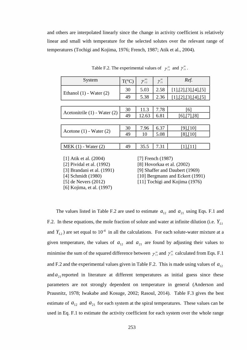
253
and others are interpolated linearly since the change in activity coefficient is relatively
linear and small with temperature for the selected solutes over the relevant range of
temperatures (Tochigi and Kojima, 1976; French, 1987; Atik et al., 2004).
Table F.2. The experimental values of 12 and .
System T(°C) Ref.
Ethanol (1) - Water (2) 30 5.03 2.58 [1],[2],[3],[4],[5]
49 5.38 2.36 [1],[2],[3],[4],[5]
Acetonitrile (1) - Water (2) 30 11.3 7.78 [6]
49 12.63 6.81 [6],[7],[8]
Acetone (1) - Water (2) 30 7.96 6.37 [9],[10]
49 10 5.08 [8],[10]
MEK (1) - Water (2) 49 35.5 7.31 [1],[11]
[1] Atik et al. (2004)
[7] French (1987)
[2] Pividal et al. (1992) [8] Hovorkaa et al. (2002)
[3] Brandani et al. (1991) [9] Shaffer and Daubert (1969)
[4] Schmidt (1980) [10] Bergmann and Eckert (1991)
[5] de Nevers (2012) [11] Tochigi and Kojima (1976)
[6] Kojima, et al. (1997)
The values listed in Table F.2 are used to estimate 12a and 21a using Eqs. F.1 and
F.2. In these equations, the mole fraction of solute and water at infinite dilution (i.e. 1LY
and 2LY ) are set equal to 10-4 in all the calculations. For each solute-water mixture at a
given temperature, the values of 12a and 21a are found by adjusting their values to
minimise the sum of the squared difference between 12 and calculated from Eqs. F.1
and F.2 and the experimental values given in Table F.2. This is made using values of 12a
and 21a reported in literature at different temperatures as initial guess since these
parameters are not strongly dependent on temperature in general (Anderson and
Prausnitz, 1978; Iwakabe and Kosuge, 2002; Rasoul, 2014). Table F.3 gives the best
estimate of and for each system at the spiral temperatures. These values can be
used in Eq. F.1 to estimate the activity coefficient for each system over the whole range
21
12
21
21
12a 21a

254
of mole fractions. However, it is useful to test the approach of finding 12a and 21a by
comparing, the prediction of the UNIQUAC model with some experimental data and that
will be discussed in the next section.
Table F.3. Binary Parameters for the studied systems estimated from the data listed in
Table F.2 and UNIQUAC equations.
System T(°C) 12a ( ) 21a ( )
Ethanol (1) - Water (2) 30 -70.16 307.91
49 -89 367.44
Acetonitrile (1) - Water (2) 30 597.71 -130.94
49 493.73 -82.9
Acetone (1) - Water (2) 30 428.95 26.06
49 672.54 10.23
MEK (1) - Water (2) 49 545.48 -5.39
F.3 Comparison with Experimental Data
To test the approach used to estimate 12a and 21a , which is based on using values of
activity coefficients at infinite dilution, a comparison is made with experimental data
available for the acetonitrile-water system at 35 °C. These data are reported in French et
al. (1987). At 35 °C, the values of 12a and 21a are estimated using 12 = 11.58 and
= 7.61 (reported in that same work) and they are found to be 410.8 K and 47.4 K,
respectively. From Eq. F.1, the activity coefficients of acetonitrile in water ( 12 ) are
estimated over the whole range of mole fraction using the values of and along
with the structural parameters of acetonitrile. Fig. F.1 shows the estimated activity
coefficients using the UNIQUAC model (dash line) and the experimental data (red
circles). As one can see, the experimental data are captured very well by the UNIQUAC
model over the whole range of mole fractions. This suggests that a reliable prediction of
the activity coefficients can be obtained using parameters derived from and .
21
12a 21a
12
21

255
0
2
4
6
8
10
12
14
0 0.1 0.2 0.3 0.4 0.5 0.6 0.7 0.8 0.9 1
YL
UNIQUAC Model
Data
Data of French et al. (1987)
12
Acetonitrile-water at 35 C
Figure F.1. Experimental activity coefficients of acetonitrile-water system at 35 °C and the
predicted values using UNIQUAC model.
F.4 Results and Comparison with UNIFAC Model
For each system, the activity coefficients at the experimental range of temperatures
are estimated using 12a and 21a listed in Table F.1. These results are shown in Fig. F.2
where the data are represented by red squares. Also, the results are compared to
corresponding values predicted by UNIFAC model. This model treats the molecules as
functional groups and has interaction parameters which are independent of temperature
(Weidlich and Gmehling, 1987). Thus, it is a pure theoretical model and provides
independent prediction of the activity coefficient and hence a reliable assessment of the
UNIQUAC model prediction can be made. UNIFAC model has many variants. However,
Dortmund-Modified UNIFAC (DMD-UNIFAC) is incorporated in ASPEN PLUS
software (version 8.4) and is chosen to achieve the comparison since it produces good
results for a large number of systems (Weidlich and Gmehling, 1987). The activity
coefficients predicted by DMD-UNIFAC model for each system at the temperature of
interest are shown in Fig. F.2 (solid line). The results show that there is a quantitate
agreement between the values predicted by the UNIQUAC model supported by
experimental data and the DMD-UNIFAC. Both models predict the activity coefficient
over the full range of mole fractions at the same degree of precision except the evident
differences over the small values of LY for acetonitrile, acetone and MEK systems at
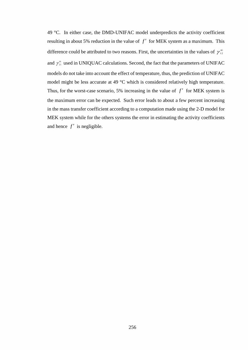
256
49 °C. In either case, the DMD-UNIFAC model underpredicts the activity coefficient
resulting in about 5% reduction in the value of for MEK system as a maximum. This
difference could be attributed to two reasons. First, the uncertainties in the values of
and used in UNIQUAC calculations. Second, the fact that the parameters of UNIFAC
models do not take into account the effect of temperature, thus, the prediction of UNIFAC
model might be less accurate at 49 °C which is considered relatively high temperature.
Thus, for the worst-case scenario, 5% increasing in the value of for MEK system is
the maximum error can be expected. Such error leads to about a few percent increasing
in the mass transfer coefficient according to a computation made using the 2-D model for
MEK system while for the others systems the error in estimating the activity coefficients
and hence is negligible.
f
12
21
f
f

257
Figure F.2. The values of the solutes activity coefficients in water predicted by the UNIQUAC
model and these by ASPEN PLUS using DMD-UNIFAC model.