Counterweight balancing for machine frame vibration ...Counterweight balancing for machine frame vibration re-duction: design and robustness analysis M. Verschuure, B. Demeulenaere,

Counterweight balancing for machine frame vibration re-duction: design and robustness analysis

M. Verschuure, B. Demeulenaere, J. Swevers, J. De SchutterK.U.Leuven, Department of Mechanical Engineering,Celestijnenlaan 300 B, B-3001, Heverlee, Belgiume-mail: [email protected]

AbstractBy addition of counterweights to the moving links of a linkage, supported by an elastically mounted frame,it is possible to reduce the frame vibration induced by the resulting forces and moments of the linkage onthe frame. Determining the counterweights that yield a maximal reduction in frame vibration is a nonlinearoptimization problem. This paper shows that this optimization problem can be reformulated as a convexproblem, i.e. a nonlinear optimization problem that has a unique (global) optimum. This methodology isgeneral but developed here for a planar four-bar linkage. For the particular example considered here, arobustness analysis shows a significant reduction of frame vibration even for drive speeds and mountingparameters other than those considered during the counterweight design.

1 Introduction

Counterweight addition is a well-known way [1, 2] to reduce the forces and moments transmitted by a linkageto its supporting frame. For planar linkages, the resulting force and moment exerted on the machine frameare denoted as the shaking force and the shaking moment. If these forces are highly peaked, troublesomevibrations in the frame might be induced. A possible side-effect of these vibrations is the transmission ofsignificant forces to the machine floor, resulting in disturbing effects in the building in which the machine isplaced as well as its surroundings [3]. Weaving mills, for instance, have been reported to cause vibration inneighboring housing blocks.

For planar four-bar linkages, which are the subject of the present paper, simultaneous elimination of theshaking force and the shaking moment requires counter-rotating masses [4] except in the case of foldablelinkages [5]. Therefore, using counterweights to reduce the reactions on the frame involves a trade-offbetween minimizing the shaking force and the shaking moment.

One approach is to minimize the shaking moment, under the restriction of complete elimination of the shak-ing force [6, 7, 8, 9, 10]. The attractive side of this full force balance approach is that the shaking momentis a pure couple and hence invariant with respect to the chosen reference point. Another approach, gearedtowards obtaining more shaking moment reduction, is to give up full force balance [11, 12, 13, 14, 15, 16,17, 18, 19, 20]. The price to be paid is that the balancing results depend on the chosen reference point forthe shaking moment.

A common weakness of both approaches is the lack of certainty whether the optimal solution actually im-proves the machine performance in terms of frame vibration. This can only be assessed if a model of theframe that supports the linkage is considered. This approach [21, 22, 23] measures the vibration level of theframe through its average kinetic energy [21, 22] and is therefore termed the energy approach to distinguishit from the full force balance approach.

3699

c2 c3

c1

o4

ϕ1

ϕ3

ϕ2

ad1

d2

o2

o1o3

c4

bqt

Figure 1: Planar crank-rocker four-bar linkage supported by an elastically mounted, rigid frame with threedegrees of freedom (qx, qy, qt). The shaded boxes indicate spring-damper systems.

The present paper considers the example of a four-bar linkage supported by an elastically mounted frame andformulates the design of the counterweights that minimize the frame vibration as an optimization problem,like in [22]. The following contributions are made. First, it is shown that the counterweight optimization canbe formulated as a convex optimization problem. Convex optimization problems are nonlinear optimizationproblems that have a unique (global) optimum, which can be found with great efficiency. Second, the numer-ical results of Kochev and Gurdev [22] are extended in several respects: a better optimum is obtained, theonly marginal beneficial effect of using a coupler counterweight is demonstrated and a robustness analysis iscarried out for drive speeds and mounting parameters, other than those considered during the counterweightdesign. Furthermore, the modeling simplifications used in [22] are validated by simulation of a completemodel using a state-of-the-art multibody simulation software (Virtual.Lab Motion1).

This paper is organized as follows. Section 2 defines the dynamic model of the machine. Section 3 developsthe balancing criteria in convex form. This method is numerically illustrated and compared with othermethods in Sec. 4. Section 5 finally discusses the obtained results, the limits of application of the methodand further research.

2 Modeling

After introducing the benchmark problem (Sec. 2.1) and the modeling assumptions (Sec. 2.2) used through-out this paper, the benchmark’s mathematical model is developed in Sec. 2.3. Subsequently, the criterium toassess the balancing results is discussed in Sec. 2.4.

2.1 Benchmark Problem

Figure 1 shows the benchmark problem [22]: a planar crank-rocker four-bar linkage supported by an elasti-cally mounted, rigid frame. The moving links as well as the frame are assumed to be rigid. The crank o1o2

(link 1) rotates at constant speed Ω (rad/s). The coupler o2o4 (link 2) connects the crank with the rocker o3o4

(link 3). The latter performs an oscillating (rocking) motion. Two linear spring-damper systems connect theframe (link 4) with the machine floor. The frame has three degrees of freedom, two translational and one

1www.lmsvirtuallab.com

3700 PROCEEDINGS OF ISMA2006

rotational, measured by the displacement

q =(qx qy qt

)T, (1)

where (.)T denotes a matrix transpose. (qx, qy) denote the coordinates of the frame center of gravity (COG)c4 with respect to the world coordinate system a. qt measures the frame rotation angle counterclockwisefrom a to the frame coordinate system b, which is attached to the frame. At rest, the frame is horizontalwith c4 coinciding with a, implying (qx, qy, qt) = (0, 0, 0). Coordinate systems with origin o are denoted aso throughout this paper.

The link coordinate systems oi, i = 1, 2, 3, are fixed to the moving links, with their abscissa alongthe link. The link angles ϕi(t) (rad) are measured counterclockwise from b to oi, whereas (xoi , yoi)measures the position of oi in b. The link lengths are denoted as ai (m).

The mass, COG and centroidal moment of inertia of each link are denoted as mi (kg), ci and Ji (kg·m2),respectively, i = 1 . . . 4. (xci , yci), i = 1 . . . 4, and (ui, vi), i = 1, 2, 3, measure the COG location inb and oi, respectively.

The spring-damper attachment points are denoted as dj , j = 1, 2 with coordinates (xdj , ydj ) in b. Thej-th spring-damper system is fully characterized by its horizontal stiffness kxj (N/m), vertical stiffness kyj

(N/m), torsional stiffness ktj (N·m/rad), horizontal viscous damping ζxj (N·s/m), vertical viscous dampingζyj (N·s/m) and torsional viscous damping ζtj (N·m·s/rad) expressed with respect to the local coordinatesystem dj parallel to a. The viscous damping coefficients are denoted using the symbol ζ instead of theclassical symbol c, used here for indicating COGs.

The shaking forces fshak,x (N) and fshak,y (N) are the x and y-component, expressed in b, of the totalforce exerted by the four-bar linkage on the supporting frame. The shaking moment mshak (N·m) is definedhere as the total moment, with respect to c4, exerted by the four-bar linkage on the frame.

2.2 Modeling Assumptions

The variation of the shaking force and the shaking moment during the motion of the linkage results in framevibration, for which a mathematical model is developed based on the following assumptions [24]:

1. rigid four-bar links and supporting frame.

2. small angular displacement qt; this implies, for instance, that the shaking force components, expressedin a are virtually identical to the shaking force components expressed in b.

3. small mass and inertia of the linkage compared to the mass and inertia of the supporting frame.

4. complete decoupling between the frame vibration and the shaking force and the shaking moment thatcause it. That is, fshak(t) and mshak(t) are determined from a kinetostatic analysis of the four-bar, inwhich the frame is considered to be at rest. This is a reasonable assumption if the previous assumptionshold and if the accelerations of the linkage pivots o1 and o3 are small with respect to the link COGaccelerations.

2.3 Mathematical Model

Based on the previously made modeling assumptions, the rigid frame vibration is governed by:

Mq(t) + Cq(t) + Kq(t) = f(t), (2)

where the components off(t) =

(fshak,x fshak,y mshak

)T (3)

ROTATING MACHINERY:DYNAMICS 3701

are considered to be exciting forces, independent from the resulting displacement q(t). These componentsare determined beforehand from a kinetostatic linkage analysis. The symmetric matrices M , C and Kdenote the mass, damping and stiffness matrices, with reference point in c4

2 and expressed with respect tothe coordinate system a:

M = diag(m4,m4, J4), C =∑

Cj , K =∑

Kj .

Kj represents the stiffness matrix of the j-th spring and Cj the damping matrix of the j-th damper:

Kj =

kxj 0 −kxj (ydj − yc4)0 kyj kyj (xdj − xc4)

−kxj (ydj− yc4) kyj (xdj

− xc4) ktj + kxj (ydj− yc4)

2 + kyj (xdj− xc4)

2

,

Cj =

ζxj 0 −ζxj (ydj− yc4)

0 ζyj ζyj (xdj − xc4)−ζxj (ydj − yc4) ζyj (xdj − xc4) ζtj + ζxj (ydj − yc4)

2 + ζyj (xdj − xc4)2

.

Since differential equation (2) is linear and its driving force periodic (with periodicity equal to the periodicityT = 2π/Ω of the linkage), its solution q is also periodic with period T .

2.4 Balancing criterium

In order to assess the balancing result, the vibration level of the machine is considered here. This balancingcriterium is measured by the average (over one period of motion) frame kinetic energy Ekin (J) [22, 21]. Theinstantaneous frame kinetic energy Ekin(t) and the numerical average kinetic energy equal

Ekin(t) =12· q(t)T ·M · q(t), (4)

Ekin =1kT

kT∑

k=1

Ekin((k − 1)Ts), (5)

where Ts (s) denotes the sampling period and kT = T/Ts denotes the number of samples per period.

3 Optimization

In order to reduce the vibration kinetic energy, counterweights are added to each link. Sections 3.2-3.4introduce the optimization variables, constraints and objective function of the original (non-convex) andreformulated convex optimization problem. Section 3.5 shows that the resulting optimization problem isconvex, more specifically a so-called second-order cone program (SOCP). First, however, Sec.3.1 introducessome basic concepts of convex optimization.

3.1 A convex optimization primer

Convex programs (CPs) are nonlinear optimization problems, for which very effective algorithms exist thatcan reliably and efficiently determine the global optimum, even for large problems. Formulating an opti-mization problem as a CP, therefore, has big advantages. Unfortunately, recognizing convex optimizationproblems, or those that can be transformed into CPs, is not straightforward: the art and challenge in convex

2In this respect, our methodology deviates slightly from [22], in which the mass, damping and stiffness matrices are referred toc, the average COG of the ensemble of the frame and the linkage. Both modeling approaches are approximate, since they are basedon the aforementioned decoupling between the frame vibration and the shaking force and shaking moment.


optimization is in problem formulation. Once a problem is formulated as a convex program, it is relativelystraightforward to solve it [25].

Several classes of CPs exist, each of which are a subclass of a more general type of problems. Starting withthe smallest class, we have: linear programs (LPs), convex quadratic programs (QPs), second-order coneprograms (SOCPs) and semidefinite programs (SDPs): LP ⊂ QP ⊂ SOCP ⊂ SDP ⊂ CP. SOCPs are ofparticular interest here. In an SOCP, one minimizes a linear objective function, subject to linear equalityconstraints, linear inequality constraints and second-order cone constraints [25]. The latter constraints are ofthe general form:

‖A · x + b‖ ≤ cT x + d, (6)

where x ∈ Rn is the optimization variable, and A ∈ Rk×n, b ∈ Rk, c ∈ Rn and d ∈ R constitute problemdata. ‖ · ‖ denotes the L2-norm: ‖x‖ =

√xT · x.

3.2 Optimization Variables

The counterweight mass parameters, indicated with an asterisk (·)∗, constitute the optimization variables,and are grouped into the optimization variable x. For a four-bar linkage:

x =(

m∗1 u∗1 v∗1 J∗1 m∗

2 u∗2 v∗2 J∗2 m∗3 u∗3 v∗3 J∗3

)T ∈ R12.

Minimizing the average kinetic energy based on these optimization variables results in a non-convex pro-gram. In order to obtain a convex program a nonlinear change of variables is required, yielding the so-calledµ-parameters [10]:

µ1i = mi;µ2i = mi · ui;µ3i = mi · vi;

µ4i = Ji + mi ·(u2

i + v2i

).

These so-called µ-parameters represent the moments of the i-th link mass distribution with respect to oi: thezeroth order moment µ1i, the x-component µ2i and y-component µ3i of the first-order moment, expressed inoi, and the second-order moment µ4i.

Two properties of the µ-parametrization are exploited here to obtain an SOCP. First, as stressed in [10], theµ-parameters are additive:

µ = µo + µ∗, (7)

where µo, µ∗ and µ group the µ-parameters (expressed in oi) of the original linkage, the counterweightsand the balanced linkage, respectively. For the four-bar example considered here, these vectors are elementsof R12 and they are given by, (·) = ∗, o,∅:

µ(·) =(

µ(·)11 µ

(·)21 µ

(·)31 µ

(·)41 µ

(·)12 µ

(·)22 µ

(·)32 µ

(·)42 µ

(·)13 µ

(·)23 µ

(·)33 µ

(·)43

)T.

This superposition principle can intuitively be understood from the fact that moments of any distribution areadditive.

Second, any force or moment obtained through a kinetostatic analysis of a linkage can be written as a linearcombination of the linkage µ-parameters, a result well-known in experimental robot identification [26]. Thisimplies that

fshak,x(t) = φx(t)T · µ, (8a)

fshak,y(t) = φy(t)T · µ, (8b)

mshak(t) = φt(t)T · µ, (8c)


where the elements of φx(t), φy(t) and φt(t) ∈ R12 are time-dependent and completely determined by thefour-bar kinematics. Analytical expressions for φx(t), φy(t) and φt(t) follow from applying the principle oflinear and angular momentum as in [27]. Note that linear independence of the elements of φx(t), φy(t) andφt(t) is not required, contrary to the linearly independent vectors introduced in [27]. Based on (8a)–(8c), (3)is written as:

f(t) = (φx(t) φy(t) φt(t))T · µ

= Φ(t)T · µ, (9)

where Φ(t) ∈ R12×3.

3.3 Constraints

Using the µ-parameters as the optimization variables requires that additional constraints be imposed to guar-antee that these variables represent a mass distribution that is realizable in theory and/or practice. Thecounterweights are required to be so-called minimum inertia counterweights, that is counterweights that arecylindrical with a radius R∗

i (m) equal to [28]:

R∗i =

√(u∗i )

2 + (v∗i )2.

Given that the centroidal moment of inertia of a cylindrical counterweight equals

J∗i =m∗

i · (R∗i )

2

2,

it follows that

J∗i =m∗

i ·((u∗i )

2 + (v∗i )2)

2. (10)

This guarantees the moment of inertia to be nonnegative provided that the counterweight mass be nonnega-tive:

m∗i ≥ 0. (11)

Furthermore, bound constraints are required for the coordinates of the center of gravity (COG) of the coun-terweights, as well as an upper limit m∗,M

tot (kg) for the total counterweight mass, in order to obtain realisticcounterweight configurations:

umi ≤ u∗i ≤ uM

i ; (12a)

vmi ≤ v∗i ≤ vM

i ; (12b)

m∗1 + m∗

2 + m∗3 ≤ m∗,M

tot . (12c)

Superscripts (·)m and (·)M denote the user-defined lower and upper bounds, respectively. Substituting theµ-parameters into (10), (11) and (12a)–(12c) yields, i = 1, 2, 3 [29]:

∥∥∥∥∥∥

√

6 · µ∗2i√6 · µ∗3i

µ∗1i − µ∗4i

∥∥∥∥∥∥≤ µ∗1i + µ∗4i; (13a)

µ∗1i · umi ≤ µ∗2i ≤ µ∗1i · uM

i ; (13b)

µ∗1i · vmi ≤ µ∗3i ≤ µ∗1i · vM

i ; (13c)

µ∗11 + µ∗12 + µ∗13 ≤ m∗,Mtot . (13d)

Equation (13a) is in fact a relaxation of (10), since the equality sign is replaced by an inequality sign.However, in all of our numerical experiments, (10) was an active constraint (i = 1, 2, 3), that is, it holds withequality. Hence, in numerical practice, (13a) and (10) are equivalent. The constraints (7) and (13a)–(13d)are linear in µ∗ji except for Eq.(13a), which is a second-order cone (SOC) constraint in µ∗1i, µ∗2i, µ∗3i and µ∗4i

as comparison with (6) reveals.


3.4 Objective function

As explained in Sec.3.2, f(t) is linear in the µ-parameters. Since Eq.(2) is a linear differential equation, itssolution q is linear in f(t) and therefore also linear in the µ-parameters:

q(t) = [qx(t) qy(t) qt(t)]T

= [ψx(t) ψy(t) ψt(t)]T · µ= Ψ(t)T · µ. (14)

The matrices ψx(t), ψy(t) and ψt(t) ∈ R12×1 are determined according to the numerical method proposedin [29]. Substituting (14) into Eq.(4) yields:

Ekin(t) =12· µT · Ψ(t)T ·M · Ψ(t) · µ

= µT ·H(t) · µ, (15)

where Ψ(t) = dΨdt . In other words: the kinetic energy can be written as a quadratic form of µ. Given the fact

that the symmetric matrix H(t) is of the form

H(t) =12· Ψ(t)T ·M · Ψ(t), (16)

with M a diagonal matrix with positive elements and Ψ(t) an arbitrary matrix (possibly not of full rank),H(t) is positive semidefinite. Substituting (15) into (5) yields:

Ekin =1kT

kT∑

k=1

µT ·Hk · µ = µT ·(∑kT

k=1 ·Hk

kT

)· µ = µT · H · µ, (17)

where Hk = H((k − 1)Ts). H is a (non-negative) sum of positive semidefinite matrices Hk and hence apositive semidefinite matrix.

3.5 Resulting SOCP

The resulting optimization problem is:

minimize[µ∗;µ] µT · H · µsubject to (7), (13a)–(13d).

SVD factorization and partitioning of the symmetric positive semidefinite matrix H yields:

H = [U1|U2] ·(

Σr 000000 000

)·[

UT1

UT2

].

Σr ∈ Rr×r is a diagonal matrix of which all diagonal elements are positive. Now introducing the auxiliaryvariables p ∈ Rr and z ∈ Rr as well as the linear equality constraints p = UT

1 · µ and z =√

Σr · p it iseasily verified that the average kinetic energy is a quadratic form E = zT · z, of a variable z that is a lineartransformation of µ.

Note that minimizing zT · z is equivalent to minimizing√

zT · z = ‖z‖ since the square root is monoto-nously increasing on the nonnegative reals. A final observation before defining the resulting SOCP is thatminimizing ‖z‖ is equivalent [25] to minimizing the auxiliary variable w subject to the (second-order cone)constraint that

‖zu‖ ≤ w. (18)


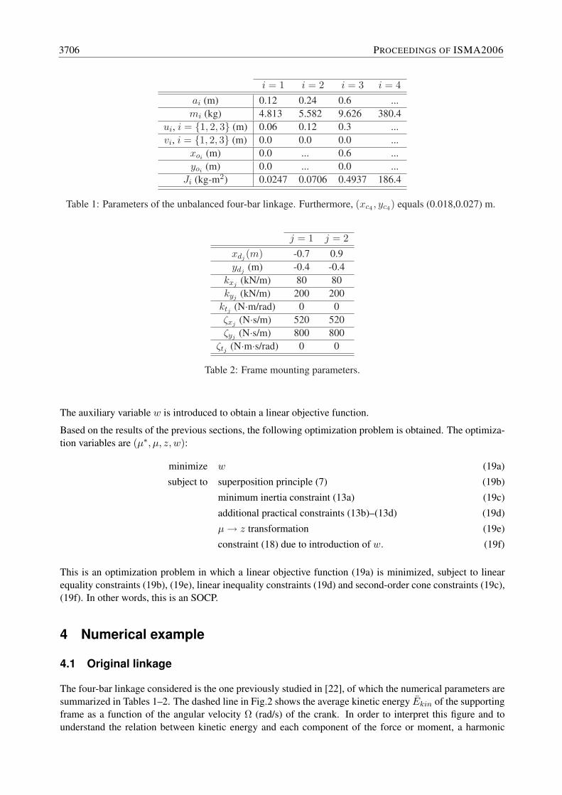
i = 1 i = 2 i = 3 i = 4ai (m) 0.12 0.24 0.6 ...mi (kg) 4.813 5.582 9.626 380.4

ui, i = 1, 2, 3 (m) 0.06 0.12 0.3 ...vi, i = 1, 2, 3 (m) 0.0 0.0 0.0 ...

xoi (m) 0.0 ... 0.6 ...yoi (m) 0.0 ... 0.0 ...

Ji (kg-m2) 0.0247 0.0706 0.4937 186.4

Table 1: Parameters of the unbalanced four-bar linkage. Furthermore, (xc4 , yc4) equals (0.018,0.027) m.

j = 1 j = 2xdj

(m) -0.7 0.9ydj

(m) -0.4 -0.4kxj (kN/m) 80 80kyj (kN/m) 200 200

ktj (N·m/rad) 0 0ζxj (N·s/m) 520 520ζyj (N·s/m) 800 800

ζtj (N·m·s/rad) 0 0

Table 2: Frame mounting parameters.

The auxiliary variable w is introduced to obtain a linear objective function.

Based on the results of the previous sections, the following optimization problem is obtained. The optimiza-tion variables are (µ∗, µ, z, w):

minimize w (19a)

subject to superposition principle (7) (19b)

minimum inertia constraint (13a) (19c)

additional practical constraints (13b)–(13d) (19d)

µ → z transformation (19e)

constraint (18) due to introduction of w. (19f)

This is an optimization problem in which a linear objective function (19a) is minimized, subject to linearequality constraints (19b), (19e), linear inequality constraints (19d) and second-order cone constraints (19c),(19f). In other words, this is an SOCP.

4 Numerical example

4.1 Original linkage

The four-bar linkage considered is the one previously studied in [22], of which the numerical parameters aresummarized in Tables 1–2. The dashed line in Fig.2 shows the average kinetic energy Ekin of the supportingframe as a function of the angular velocity Ω (rad/s) of the crank. In order to interpret this figure and tounderstand the relation between kinetic energy and each component of the force or moment, a harmonic


5 10 15 20 25 30 35 40 45 50 55 6010

−4

10−3

10−2

10−1

100

101

102

Ω [rad/s]

Eki

n [J]

original

optimized

Figure 2: Average frame kinetic energy versus crankspeed for the original linkage (dashed line) and theoptimized linkage (solid line) with the three counterweights of Table 4–column 6.

umi (m) uM

i (m) vmi (m) vM

i (m)i = 1, (a1 = 0.12m) -0.0761 0.0600 -0.0300 0.0212i = 2, (a2 = 0.24m) -0.1200 0.1200 -0.1200 0.1200i = 3, (a3 = 0.60m) -0.1500 0.1500 -0.1000 0.1000

Table 3: Upper and lower bounds on the counterweight COG coordinates.

analysis is carried out. The three (damped) resonance frequencies of the 3-dof flexibly mounted frame equal:

ωn1 = 19.04 rad/s, ωn2 = 31.98 rad/s, ωn3 = 40.11 rad/s. (20)

The peaks in the average kinetic energy emerge if Ω is such that one of the harmonics is close to one of theresonance frequencies. For instance in the case of the peak near Ω = 19 rad/s and Ω = 32 rad/s, the firstharmonic of Ω is close to ωn1 and ωn2, respectively. For the peak near Ω = 9.5 rad/s the second harmonic isclose to ωn1. In this example counterweights are designed for a crank speed of Ω = 20 rad/s as in [22]. Table3 shows the values for the upper and lower bounds on the COG coordinates used in (13b)-(13c), i = 1, 2, 3.These values are chosen such that the counterweights of [22] comply with them3.

The upper limit m∗,Mtot on the total counterweight mass is set to 24.25 kg, that is, exactly the amount of

counterweight mass used in [22]. This mass corresponds to about 1/16 of the frame mass and 1.2 times theoriginal four-bar mass.

The optimization problem is implemented in Matlab, using Yalmip, a Matlab toolbox for modelingoptimization problems independently of the numerical solver [30]. The SOCP numerical solver used hereis SeDuMi, a dedicated software package for optimization problems over symmetric cones [31]. Solvingone optimization problem instance does not require an initial guess and on average takes less than one CPUsecond.

4.2 Results

Table 4 shows the results of the optimization for different objective functions and optimization methods.Optimizations have been carried out with Gurdev and Kochev’s reference point c (see Sec. 2.2) and thereference point c4 used here.

3It would be more accurate to use the bounds chosen in [22], but these bounds are not provided in this reference.


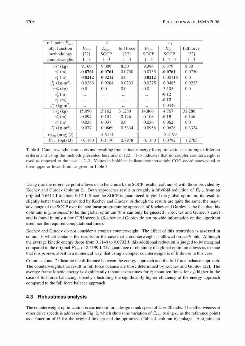
ref. point Ekin c c4

obj. function Ekin Ekin full force Ekin Ekin full forcemethodology [22] SOCP [22] SOCP SOCP [22]

counterweights 1 - 3 1 - 3 1 - 3 1 - 3 1 - 2 - 3 1 - 3m∗

1 (kg) 9.160 9.089 8.30 9.384 16.379 8.30u∗1 (m) -0.0761 -0.0761 -0.0750 -0.0735 -0.0761 -0.0750v∗1 (m) 0.0212 0.0212 0.0 0.0212 0.00116 0.0

J∗1 (kg-m2) 0.0286 0.0284 0.0233 0.0275 0.0485 0.0233m∗

2 (kg) 0.0 0.0 0.0 0.0 3.105 0.0u∗2 (m) ... ... ... ... -0.12 ...v∗2 (m) ... ... ... ... -0.12 ...

J∗2 (kg-m2) ... ... ... ... 0.0447 ...m∗

3 (kg) 15.090 15.162 31.280 14.866 4.767 31.280u∗3 (m) -0.094 -0.101 -0.146 -0.108 -0.15 -0.146v∗3 (m) 0.036 0.037 0.0 0.036 0.062 0.0

J∗3 (kg-m2) 0.077 0.0869 0.3334 0.0956 0.0628 0.3334Ekin (orig) (J) 5.6414 8.4199Ekin (opt) (J) 0.1180 0.1170 0.7978 0.1140 0.0792 1.2705

Table 4: Counterweight parameters and resulting frame kinetic energy for optimization according to differentcriteria and using the methods presented here and in [22]. 1–3 indicates that no coupler counterweight isused as opposed to the case 1–2–3. Values in boldface indicate counterweight COG coordinates equal totheir upper or lower limit, as given in Table 3.

Using c as the reference point allows us to benchmark the SOCP results (column 3) with those provided byKochev and Gurdev (column 2). Both approaches result in roughly a fiftyfold reduction of Ekin from anoriginal 5.6414 J to about 0.12 J. Since the SOCP is guaranteed to yield the global optimum, its result isslightly better than that provided by Kochev and Gurdev. Although the results are quite the same, the majoradvantage of the SOCP over the nonlinear programming approach of Kochev and Gurdev is the fact that thisoptimum is guaranteed to be the global optimum (this can only be guessed in Kochev and Gurdev’s case)and is found in only a few CPU seconds (Kochev and Gurdev do not provide information on the algorithmused, nor the required computational time).

Kochev and Gurdev do not consider a coupler counterweight. The effect of this restriction is assessed incolumn 6 which contains the results for the case that a counterweight is allowed on each link. Althoughthe average kinetic energy drops from 0.1140 to 0.0792 J, this additional reduction is judged to be marginalcompared to the original Ekin of 8.4199 J. The guarantee of obtaining the global optimum allows us to statethat it is proven, albeit in a numerical way, that using a coupler counterweight is of little use in this case.

Columns 4 and 7 illustrate the difference between the energy approach and the full force balance approach.The counterweights that result in full force balance are those determined by Kochev and Gurdev [22]. Theaverage frame kinetic energy is significantly (about seven times for c; about ten times for c4) higher in thecase of full force balancing, thereby illustrating the significantly higher efficiency of the energy approachcompared to the full force balance approach.

4.3 Robustness analysis

The counterweight optimization is carried out for a design crank speed of Ω = 20 rad/s. The effectiveness atother drive speeds is addressed in Fig. 2, which shows the variation of Ekin (using c4 as the reference point)as a function of Ω for the original linkage and the optimized (Table 4–column 6) linkage. A significant


kx [N/m]

k y [N/m

]

0.5 1 1.5 2 2.5 3 3.5 4

x 105

0.5

1

1.5

2

2.5

3

3.5

4x 10

5

2

4

6

8

10

12

(a) original linkage

kx [N/m]

k y [N/m

]

0.5 1 1.5 2 2.5 3 3.5 4

x 105

0.5

1

1.5

2

2.5

3

3.5

4x 10

5

0.2

0.4

0.6

0.8

1

1.2

1.4

1.6

1.8

2

(b) optimized linkage with the three counterweightsof Table 4–column 6

Figure 3: Average frame kinetic energy for different damping values of kx and ky and for ζx = 520 Ns/mand ζy = 800 Ns/m at a crankspeed of 20 rad/s.

frame vibration reduction is observed over the entire speed range, which illustrates the robustness of thecounterweight design, despite that robustness is not taken into account during the design stage.

Furthermore, the effect of variation of the stiffness values kx,i and ky,i on the resulting average kinetic energyis investigated in Fig. 3 for the damping values given in Table 2. Since both spring-damper systems are thesame it suffices to consider the variation of kx,i = kx, i = 1, 2 and ky,i = ky, i = 1, 2. The analysis iscarried out for kx and ky values ranging from 20 kN/m to 400 kN/m, i.e. a maximum stiffness of about 5times the design value of kx and of 2 times the design value of ky. For these values of kx and ky, Fig.3(a)and (b) show the average kinetic energy of the original linkage and the optimized linkage, respectively.

In Fig.3(a) two regions with significantly higher vibration levels appear, one around kx = 100 kN/m and onearound ky = 80 kN/m. For these stiffness values, one of the frame resonance frequencies gets very close tothe first harmonic frequency of the shaking force/moment (20 rad/s), which explains the increased vibrationlevel. More specifically, the frame resonance frequency of 20 rad/s around kx = 100 kN/m, is mainly excitedby the first harmonic of fshak,x, while the frame resonance frequency of 20 rad/s around ky = 80 kN/m, ismainly excited by the first harmonic of fshak,y.

In Fig.3(b), the increased vibration region around kx = 100 kN/m has disappeared. This is due to factthat the counterweights result in a 17-fold reduction of the first harmonic of fshak,x. On the other hand,the first harmonic of fshak,y is reduced with a factor of two only, which clearly does not suffice to removethe increased vibration region around ky = 80 kN/m. The reduction of the first harmonics of fshak,x andfshak,y comes at a cost of an increased first and second harmonic of mshak. This, however, does not resultin increased frame vibration, which is illustrated by the fact that the counterweights reduce (compared to theoriginal linkage) the average kinetic energy with 45% to 99.9% for all considered values of stiffness.

For the stiffness values given in Table 2, Fig. 4(a) and (b) show the average kinetic energy of the originallinkage and the optimized linkage, respectively, for different values of ζx and ζy. Since both spring-dampersystems are the same, they are both varied in the same way. A range from 0 to 1600 N· s/m is considered forboth ζx and ζy, i.e. a maximum damping of about 3 times the design ζx and of 2 times the design ζy. Figure4(b) shows that the average kinetic energy of the optimized linkage changes little over the whole range. Thisis due to the fact that changing the damping has a much smaller effect on the (damped) resonance frequenciesthan changing the stiffness. For the damping range considered here, the first harmonics of fshak,x and fshak,y

never coincide exactly with the frame resonance frequencies, resulting in lower vibration levels in Fig. 4(b)than in 3(b).

It can therefore be concluded that, for this particular example, counterweight balancing is a very robustsolution for vibration reduction, both for changes in crank speed, damping and stiffness. More examples are


ζx [Ns/m]

ζ y [Ns/

m]

0 200 400 600 800 1000 1200 1400 16000

200

400

600

800

1000

1200

1400

1600

4

6

8

10

12

14

16

18

20

22


ζx [Ns/m]

ζ y [Ns/

m]

0 200 400 600 800 1000 1200 1400 16000

200

400

600

800

1000

1200

1400

1600

0.08

0.09

0.1

0.11

0.12

0.13

0.14

0.15


Figure 4: Average frame kinetic energy for different damping values of ζx and ζy and for kx = 80 kN/m andky = 200 kN/m at a crankspeed of 20 rad/s.

0 0.05 0.1 0.15 0.2 0.25 0.3

2

4

6

8

10

12

14

16

time [sec]

E0 ki

n [J]

Virtual.LabMatlab


0 0.05 0.1 0.15 0.2 0.25 0.3

0.02

0.04

0.06

0.08

0.1

0.12

0.14

0.16

0.18

0.2

0.22

time [sec]

Eki

n [J]

Virtual.LabMatlab


Figure 5: Instantaneous frame kinetic energy during one period of motion for the exact Virtual.Lab simula-tion (solid line) and the approximate Matlab simulation (dashed line).

needed, however, to draw more general conclusions regarding robustness. In addition, future work will focuson including robustness in the optimization framework.

4.4 Validation of the model

In this section, the validity of the modeling assumptions of Sec.2.2 is assessed by comparing the approximatemodeling results with those obtained from a state-of-the-art multibody simulation software (Virtual.LabMotion). Figure 5(a) shows the frame kinetic energy during one period of motion of the original linkagefor the exact Virtual.Lab simulation (solid line) and the approximate Matlab simulation (dashed line). Figure5(b) shows the same simulation results for the optimized linkage of Table 4-column 6 (reference point c4).At Ω = 20 rad/s, the resulting relative error on the average frame kinetic energy is 52% for the originallinkage and 1% for the balanced linkage. Using c as in [22] gives a better estimation: relative errors of 3%(Ekin) for the original linkage. Near the optimum both methods provide a similar estimation, however.

The model is significantly more accurate for the balanced linkage since it satisfies the assumptions ofSec.2.2 to a much greater extent. First, the small angular displacement assumption is much better fulfilled:max(|qt|) = 5 · 10−3 rad (original) versus max(|qt|) = 5 · 10−4 rad (balanced). Second, the assumption


of small pivot accelerations is met to a much greater extent since the maximum absolute value of the frameacceleration (qx, qy, qt) drops significantly: from (11.2 m/s2, 3.8 m/s2, 5.3 rad/s2) to (1.0 m/s2, 1.9 m/s2, 1.2rad/s2).

5 Discussion and conclusion

It has been shown that counterweight balancing by minimizing the average frame kinetic energy can beformulated (under not too restrictive modeling assumptions) as a convex optimization problem, which guar-antees that the global optimum be found. This methodology has been successfully applied to an earlierbenchmark by Kochev and Gurdev: their results have been (slightly) improved, by solving an SOCP thatrequires only a few seconds of computational time. For the same example, the balancing has been shown tobenefit only marginally from using a coupler counterweight. This balancing results in a significant reductionof the frame kinetic energy, even for drive speeds and stiffness and damping values other than those used foroptimization.

The presented method is easily applied to more complicated mechanisms. It is applicable to any planarlinkage, mounted on springs and dampers with linear characteristics. The example used a constant inputspeed of the crank but this method also applies to any periodic movement of the crank. The authors feel thatconsidering more complicated mechanisms will better demonstrate the potential of the method, since thereis a much bigger chance (due to the increased number of optimization variables) to get trapped in a localoptimum for the nonconvex optimization problem formulation proposed by Kochev and Gurdev.

Some assumptions were made which limit the application of this method. First, it is not possible to evaluatethe potential of this method for machines where the frame vibrations significantly influence the forces in themechanism and where the total mass of the mechanism is close to the mass of the frame (this is only rarelythe case, however). Second, the four-bar links and the frame are assumed to be rigid. While link elasticityconstitutes a dramatic complication, frame elasticity can also be accounted for in the present framework.Third, the results of the optimization depend on the parameters of the frame mounting.

Present research is focusing on (i) including robustness for varying mounting parameters in the presentframework, (ii) extending the present framework to also include the transmission of forces to the machinefloor and (iii) illustrating the application potential for more complicated mechanisms.

Acknowledgment

This work has been carried out within the framework of project G.0462.05 ‘Development of a powerfuldynamic optimization framework for mechanical and biomechanical systems based on convex optimizationtechniques’ of the Research Foundation - Flanders (FWO - Vlaanderen). Bram Demeulenaere is a Post-doctoral Fellow of the Research Foundation - Flanders (FWO–Vlaanderen). The support of the followingprojects is gratefully acknowledged: IWT 040444 ’Dynamic Balancing of Weaving Machines’ of the Insti-tute for the Promotion of Innovation by Science and Technology in Flanders (IWT) and K.U.Leuven-BOFEF/05/006 Center-of-Excellence Optimization in Engineering.

References

[1] G.G. Lowen, F.R. Tepper, and R.S. Berkof. Balancing of linkages–an update. Mechanism and MachineTheory, 18(3):213–220, 1983.

[2] V.H. Arakelian and M.R. Smith. Shaking force and shaking moment balancing of mechanisms: A his-torical review with new examples. Transactions of the ASME, Journal of Mechanical Design, 127:334–339, 2005.


[3] G.H. Martin. Kinematics and Dynamics of Machines (2nd Ed.). McGraw-Hill, 1982.

[4] R.S. Berkof. Complete force and moment balancing of inline four-bar linkages. Mechanism andMachine Theory, 8:397–410, 1973.

[5] C.M. Gosselin, F. Vollmer, G. Cote, and Y. Wu. Synthesis and design of reactionless three-degree-of-freedom parallel mechanisms. IEEE Transactions on Robotics and Automation, 20(2), April 2004.

[6] R.S. Berkof and G.G. Lowen. Theory of shaking moment optimization of force-balanced four-barlinkages. Transactions of the ASME, Journal of Engineering for Industry, pages 53–60, 1971.

[7] G.G. Lowen and R.S. Berkof. Determination of force-balanced four-bar linkages with optimum shakingmoment characteristics. Transactions of the ASME, Journal of Engineering for Industry, pages 39–46,1971.

[8] J.L. Wiederrich and B. Roth. Momentum balancing of four-bar linkages. Transactions of the ASME,Journal of Engineering for Industry, pages 1289–1295, 1976.

[9] W.L. Carson and J.M. Stephens. Feasible parameter design spaces for force and root-mean-squaremoment balancing an in-line 4r 4-bar synthesized for kinematic criteria. Mechanism and MachineTheory, 13:649–658, 1978.

[10] R.S. Haines. Minimum rms shaking moment or driving torque of a force-balanced 4-bar linkage usingfeasible counterweights. Mechanism and Machine Theory, 16:185–190, 1981.

[11] B. Porter and D.J Sanger. Synthesis of dynamically optimal four-bar linkages. Proc. Conf. Mechanisms1972, Paper No. C69/72:24–28, Institution of Mechanical Engineers, 1972.

[12] J.P. Sadler and R.W. Mayne. Balancing of mechanisms by nonlinear programming. 3rd Applied Mech-anism Conference, Paper No. 29, Oklahoma State University, Stillwater, Oklahoma, 1973.

[13] F.R. Tepper and G.G. Lowen. Shaking force optimization of four-bar linkage with adjustable constraintson ground bearing forces. Transactions of the ASME, Journal of Engineering for Industry, pages 643–651, 1975.

[14] H. Dresig and S. Schonfeld. Rechnergestutzte optimierung der antriebs- und gestellkraftgrossen ebenerkoppelgetriebe (computer-aided optimization of driving and frame reaction forces of planar linkages).Mechanism and Machine Theory, 11(6):363–379, 1976.

[15] S.J. Tricamo and G.G. Lowen. Simultaneous optimization of dynamic reactions of a four-bar linkagewith prescribed maximum shaking force. Transactions of the ASME, Journal of Mechanisms, Trans-missions, and Automation in Design, 105:520–525, 1983.

[16] T.W. Lee and C. Cheng. Optimum balancing of combined shaking force, shaking moment, and torquefluctuations in high-speed linkages. Transactions of the ASME, Journal of Mechanisms, Transmissions,and Automation in Design, 106:242–251, 1984.

[17] N.M. Qi and Pennestri. E. Optimum balancing of four-bar linkages–a refined algorithm. Mechanismand Machine Theory, 26(3):337–348, 1991.

[18] Porter. B., S.S. Mohamed, and B.A. Sangolola. Genetic design of dynamically optimal four-bar link-ages. In Proceedings of the 1994 ASME Mechanisms Conference, volume DE–70, pages 413–424,Minneapolis, Minnesota, 1994.

[19] G. Guo, N. Morita, and T. Torii. Optimum dynamic design of planar linkage using genetic algorithms.JSME International Journal, Series C: Mechanical Systems, Machine Elements and Manufacturing,43(2):372–377, 2000.


[20] B. Demeulenaere, E. Aertbelien, M. Verschuure, J. Swevers, and J. De Schutter. Ultimate limits forcounterweight balancing of crank-rocker four-bar linkages. Accepted for Publication in ASME J. ofMech. Design.

[21] W.E. Johnson and N.Y. Schenectady. A method of balancing reciprocating machines. Transactions ofthe ASME, Journal of Applied Mechanics, 57:A81–A86, 1935.

[22] I.S. Kochev and G.H. Gurdev. General criteria for optimum balancing of combined shaking force andshaking moment in planar linkages. Mechanism and Machine Theory, 23(6):481–489, 1988.

[23] S. Zhang and J. Chen. The optimum balance of shaking force and shaking moment of linkage. Mecha-nism and Machine Theory, 30:589–597, 1995.

[24] I.S. Kochev. A new general method for full force balancing of planar linkages. Mechanism and MachineTheory, 23(6):475–480, 1988.

[25] S. Boyd and L. Vandenberghe. Convex Optimization. Cambridge University Press, 2004.

[26] C.G. Atkeson, C.H. An, and J.M. Hollerbach. Estimation of inertial parameters of manipulator loadsand links. The International Journal of Robotics Research, 5(3):101–119, 1986.

[27] R.S. Berkof and G.G. Lowen. A new method for completely force balancing simple linkages. Trans-actions of the ASME, Journal of Engineering for Industry, pages 21–26, 1969.

[28] F.R. Hertrich. How to balance high-speed mechanisms with minimum inertia counterweights. MachineDesign, 35(6):160–164, 1963.

[29] B. Demeulenaere. Dynamic Balancing of Reciprocating Machinery With Application to Weaving Ma-chines. PhD thesis, Dept. of Mech. Eng., K.U.Leuven, Leuven, Belgium, 2004.

[30] J Lofberg. Yalmip : A toolbox for modeling and optimization in matlab. In Proc. 2004 IEEECCA/ISIC/CACSD, page Paper SaM09.1, Taipei, Taiwan, 2004.

[31] J.F. Sturm. Using sedumi 1.02, a matlab toolbox for optimization over symmetric cones. OptimizationMethods and Software, 11–12:625–653, 1999. Special issue on Interior Point Methods (CD supplementwith software).



Documents

Counterweight balancing for machine frame vibration ...Counterweight balancing for machine frame vibration re-duction: design and robustness analysis M. Verschuure, B. Demeulenaere,