Counting on b-Diversity to Safeguard the Resilience of Estuaries

Counting on b-Diversity to Safeguard the Resilience ofEstuariesSilvia de Juan*, Simon F. Thrush, Judi E. Hewitt

National Institute of Water and Atmospheric Research, Hamilton, New Zealand

Abstract

Coastal ecosystems are often stressed by non-point source and cumulative effects that can lead to local-scale communityhomogenisation and a concomitant loss of large-scale ecological connectivity. Here we investigate the use of b-diversity asa measure of both community heterogeneity and ecological connectivity. To understand the consequences of differentenvironmental scenarios on heterogeneity and connectivity, it is necessary to understand the scale at which differentenvironmental factors affect b-diversity. We sampled macrofauna from intertidal sites in nine estuaries from New Zealand’sNorth Island that represented different degrees of stress derived from land-use. We used multiple regression models toidentify relationships between b-diversity and local sediment variables, factors related to the estuarine and catchmenthydrodynamics and morphology and land-based stressors. At local scales, we found higher b-diversity at sites with arelatively high total richness. At larger scales, b-diversity was positively related to c-diversity, suggesting that a largeregional species pool was linked with large-scale heterogeneity in these systems. Local environmental heterogeneityinfluenced b-diversity at both local and regional scales, although variables at the estuarine and catchment scales were bothneeded to explain large scale connectivity. The estuaries expected a priori to be the most stressed exhibited higher variancein community dissimilarity between sites and connectivity to the estuary species pool. This suggests that connectivity andheterogeneity metrics could be used to generate early warning signals of cumulative stress.

Citation: de Juan S, Thrush SF, Hewitt JE (2013) Counting on b-Diversity to Safeguard the Resilience of Estuaries. PLoS ONE 8(6): e65575. doi:10.1371/journal.pone.0065575

Editor: Matteo Convertino, University of Florida, United States of America

Received March 9, 2013; Accepted April 27, 2013; Published June 5, 2013

Copyright: � 2013 de Juan et al. This is an open-access article distributed under the terms of the Creative Commons Attribution License, which permitsunrestricted use, distribution, and reproduction in any medium, provided the original author and source are credited.

Funding: SdJ was funded by a postdoctoral mobility grant from The Spanish Ministry of Education (Programa nacional de movilidad de recursos humanos delPlan Nacional I+D+i 2008–2011). This work was supported by funding from MBIE (NIWA COMS1302, COER1201 & C01X0501). The funders had no role in studydesign, data collection and analysis, decision to publish, or preparation of the manuscript.

Competing Interests: The co-author Simon Thrush is a PLOS ONE Academic Editor. However, this does not imply any competing interests and it does not alterthe authors’ adherence to all the PLOS ONE policies on sharing data and materials.

* E-mail: [email protected]

Introduction

The effects of spatial scale on diversity are readily apparent from

species accumulation curves that are structured by increasing the

sampling area or the number of habitats [1,2]. This implies a

strong interaction between the regional species pool and the local

richness. b-diversity can represent the difference in species

composition between local and regional assemblages [3] and in

this context it reflects heterogeneity in community composition

and ecological connectivity [4–6]. Under this definition, b-

diversity has been suggested as a measure of ecosystem resilience

across scales [7], where the difference between a local site’s

richness and the size of the regional species pool reflects the

connectivity between biological assemblages and thus influences

the recovery potential of ecological systems [6,8]. However,

cumulative disturbance can cause both ecological and physical

habitat fragmentation and local community homogenisation, with

the consequent loss of ecological connectivity feeding back on the

potential for recovery [8,9]. Habitat homogenisation and ecolog-

ical fragmentation are amongst the main threats to biodiversity

[10], and b-diversity has been promoted as providing essential

information for conservation management by highlighting the

consequences of biodiversity loss to ecosystem resilience [6,11,12].

Under the current global situation of marine ecosystem

degradation due to cumulative stressors [13], we need to

identify and test surrogate variables that indicate the potential

for dynamic changes in community state. In this context, b-

diversity is essential for identifying relevant scales of change and

understanding ecosystem processes related to anthropogenic

activities [6,14]. A range of natural factors have been implicated

in affecting changes in b-diversity patterns, including distance

between locations and mechanisms related to dispersal, local

environmental variability and changes in the strength of species

interaction [15–17]. Empirical evidence for the relative impor-

tance of these factors is inconsistent [18] and it is likely to vary

over space and time scales [6]. Human activities can also have

different effects on patterns in b-diversity at different scales, e.g.

at local scales stress could decrease heterogeneity [19] while at

regional scales it could initially increase heterogeneity through

the loss of ecological connectivity, i.e. ecological fragmentation

[7,10]. Importantly, b-diversity may show non-linear responses

to stress, as diffuse sources of anthropogenic disturbance can

operate in a cumulative fashion, implying the importance of

understanding thresholds of change in b-diversity [9,20].

While our ability to identify abrupt regime shifts in natural

systems has improved, detection of potential early-warning signals

is still very limited [21–23]. At present, the only way of detecting a

threshold is to cross it [24] and thus identifying indicators and

trends that occur in advance of large shifts in ecosystem state is

critical for successful management, especially if there is hysteresis

PLOS ONE | www.plosone.org 1 June 2013 | Volume 8 | Issue 6 | e65575

in recovery dynamics [25]. Early warning signals for regime shifts

would be useful for managing transitions, however, response

patterns still remain ambiguous limiting application in manage-

ment. While most of the proposed indicators are theoretically well

developed, there have been few empirical tests [26–28], but see

[23,29], with effective long-term time-series monitoring required

[21,29,30]. In this context, there is a need to understand

connectivity and heterogeneity patterns before systems transition

to a degraded state. However, the expected responses to

disturbance may not be evident in low stress scenarios as

heterogeneity between locations and habitat types would maintain

the regional species pool [30]. This suggests that there is likely to

be a threshold to the effects of habitat fragmentation on b-

diversity, when habitat patches are too small and unconnected to

sustain viable populations [2] and thus the regional species pool

decreases, causing broad-scale homogeneity [10] and low b-

diversity at medium to large scales. b-diversity is also a promising

measure of ecosystem integrity, but its use needs to be verified by

testing for scale-dependence in relation to disturbance.

The estuaries in New Zealand can be considered low stressed

systems (compared to more populated regions) and we aimed to

assess local and regional scales of heterogeneity and ecological

connectivity in these systems. In a naturally heterogeneous

estuarine system we would expect local connectivity patterns

(connecting patches on the 10–100 m scale) to be strongly

influenced by micro-scale environmental variability, while at

larger scales we would expect estuarine morphology and

hydrodynamics to increase in importance, although these different

scales will interact [2,6,31,32]. Diffuse sources of stress in these

estuaries are mainly caused by land-based environmental stressors

that include runoff from agricultural, industrial and urban land-

use [10,33,34] modified by the size and topography of the

catchment as well as by climate. Once some understanding of the

scale-dependence of environmental factors that contribute to

ecological connectivity and heterogeneity has been gained,

exploring changes in b-diversity should provide information about

the subtle effects of human disturbance in estuaries, such as

changes in small-scale patchiness [10] and loss of connectivity

between ecological units [6].

Here we consider three hypotheses related to spatial scale, land-

use stressors and b-diversity: (1) Within-site small-scale heteroge-

neity in species richness primarily depends on local environmental

variables. (2) The estuarine community heterogeneity and

connectivity among communities (between-sites scale) is primarily

controlled by large-scale changes in estuarine characteristics and

the within estuary habitat variability. (3) Heterogeneity and

connectivity patterns are controlled by stress derived from human

uses in the estuary causing small-scale homogeneity, resulting in

ecological fragmentation and consequent large-scale loss of

connectivity. The alternative hypotheses imply that the heteroge-

neity and connectivity patterns are controlled by distance between

locations that determines connectivity among communities

through species’ dispersal patterns. This study employs a novel

approach based on the empirical study of b-diversity patterns

across scales, from local patches to regional scales, compared to

most studies which focus on a single scale. Using this approach we

aim to assess shifts in scale-dependent heterogeneity and

connectivity in systems subjected to a gradient of diffuse source

stressors.

Materials and Methods

Characterisation of the EstuariesA set of nine estuaries with different intensities of land-based

stressors were selected around the North Island of New Zealand

(Fig. 1): Parekura, Whananaki, Okura, Puhoi, Waiwera, Whanga-

teau, Mangemangeroa, Tamaki and Waitemata. In order to

identify variability between estuaries linked to natural or

anthropogenic factors, a range of potential explanatory variables

for changes in b-diversity were obtained from existing data bases

and sampling. These variables covered local (site), within estuary,

and estuary/catchment scales. The estuarine and catchment

characteristics were available from the New Zealand Estuarine

Environment Classification Database (NZEED, [35]). The per-

centage of land cover in the catchment of natural, pastoral and

exotic (i.e. plantation forests) vegetation and urbanisation were

used as surrogates for stress caused by human uses in the

catchment [33,36]. Tamaki and Waitemata estuaries were

expected to be the most stressed as the percentage of urban cover

was over 40%, while Parekura and Whananaki had the largest

proportion of natural cover in the catchment (Table 1). The

estuaries also exhibited variable morphology and hydrodynamics

(Table 1), although they were all coastal-ocean dominated systems

with low freshwater input relative to the tidal exchange. The Shore

Complexity Index (as the length of the perimeter of the estuary

shoreline divided by the circumference of a circle that has the

same area as the estuary; 1 for simple and ,0.1 for complex

shoreline) and the Closure Index (as the width of the estuary

mouth divided by the length of the perimeter of the estuary

shoreline; 0.4 wide mouth to ,0.01 narrow entrance), were also

available from NZEED. Total nitrogen and ammoniacal-nitrogen

as annual average loads to each estuary were available (http: //

www.mpi.govt.nz/environment-natural-resources/water/clues),

but preliminary analyses showed no effects of these parameters on

the b-diversity measures and were not included further.

Sampling SitesThe estuaries were sampled in spring-summer between 2006

and 2011: summer 2006 and 2009 in Waitemata, spring-summer

2009 and 2010 in Tamaki, spring 2011 in Mangemangeroa and

summer 2008 in the other estuaries. However, for all sites not

sampled in the summer of 2008 (i.e. some sites from Waitemata,

Tamaki and Mangemangeroa), time series of macrofaunal and

sediment composition at most sites within the estuary were

available over a 5 year period and multivariate analysis of these

variables did not show a strong annual variation relative to within

or between estuarine differences. For example, 7 of the 10 sites in

Mangemangeroa had been sampled in every year since 2005 in

early spring and late summer and we tested that differences in

community composition based on presence/absence data between

these 7 sites did not differ between the 2011 year and the others,

and that late summer sampling was not different to early spring.

Between 9 and 10 randomly located intertidal sandy sites were

sampled in each estuary, with the exception of Okura, 8 sites,

Whananaki, 6 sites, and Tamaki, 7 sites. Ten core samples of

13 cm of diameter and 15 cm depth were obtained at each site

(with the exception of Mangemangeroa where only 6 samples were

available). This sampling strategy covered the within-patch

heterogeneity with 6–10 replicates obtained at each site (site area

c 50 m2), and the within estuary heterogeneity, by sampling 10

sites across sand-flats with variable sand-mud content. Distance

between sites varied from an average of 15.7 km in Waitemata to

0.4 km in Mangemangeroa (Appendix 1), related to the size of the

estuary.

b-Diversity and the Resilience of Estuaries


Core samples were sieved through a 500 mm mesh and the

retained organisms were identified to the lowest practical

taxonomical level (generally species). Small cores (2 cm depth)

were used to sample surface sediment for grain size, organic

content and benthic chlorophyll a at each site (organic content was

not available for Waitemata and Tamaki and chlorophyll a was

not available for Mangemangeroa and Tamaki). The presence of

shell hash was assessed at each site, based on visual assessment of

shell material present on the sediment surface within 5 0.25 m2

quadrat photos, as: no shell (0%), rare (0–5%) and presence when

there was a moderate to high abundance (.5% and it was rarely

higher than 40%).

No specific permissions were required for sampling these

locations as our sampling is a permitted activity. Field studies

did not involve endangered or protected species.

b-diversity MeasuresNumerous studies have addressed the importance of b-diversity

to ecological patterns by using a great variety of metrics; a

consensus has not been reached and variety of metrics prevail

Figure 1. Map of the study area: 9 estuaries in New Zealand North Island.doi:10.1371/journal.pone.0065575.g001

Table 1. Estuarine and catchment characteristics.

EstuariesEstuaryarea

Catchmentarea

Shorelength SC CI

Riverinflow

Riverdischarge Rainfall Runoff

Tiderange

Intertidal(%)

Natural(%)

Pastoral(%)

Urban(%)

Exotic(%)

Mangemangeroa 0.6 10.0 7.4 0.34 0.09 0.02 0.4 1208 300 2.4 86.9 26.6 69.9 3.4 0.09

Okura 1.4 27.4 12.7 0.31 0.04 0.06 1.2 1401 457 2.2 79.3 40.7 36.9 0.6 21.8

Parekura 3.6 23.2 14.4 0.45 0.05 0 1.2 1598 664 1.6 36.9 77.3 17.1 0 5.6

Puhoi 1.7 43.0 18.7 0.25 0 0.03 2.2 1600 764 2.1 70.6 32.8 55.5 0 11.4

Tamaki 16.9 108.8 94.6 0.15 0.02 0.004 4.1 1208 250 2.4 40.0 1.96 24.7 73.1 0.2

Waitemata 78.8 427.3 260.1 0.12 0.01 0.003 19.7 1468 430 2.3 36.2 18.6 34.5 42.6 4.2

Waiwera 1.0 37.9 11.7 0.3 0.001 0.04 1.9 1577 643 2.1 64.5 47.1 52.3 0.4 0.3

Whananaki 2.1 53.9 16.8 0.3 0.01 0.04 2.9 1731 778 1.6 75.3 65.1 34.5 0 0.2

Whangateau 7.5 42.4 31.9 0.3 0.01 0.01 2.1 1596 553 1.9 85.4 19.6 75.6 0.9 3.6

Data obtained from the New Zealand Estuarine Environment Classification Database [35].Estuarine water area at high tide and land catchment area in km2. Shore length in km. The shore complexity index (SC) as the length of the perimeter of the estuaryshoreline divided by the circumference of a circle that has the same area as the estuary (1 simple and ,0.1 complex shoreline). The closure index (CI) as the width of theestuary mouth divided by the length of the perimeter of the estuary shoreline (0.4 wide to ,0.01 narrow entrance). Annual river inflow as the ratio of river inflow tototal estuary volume at high water. The mean annual discharge of river to estuary in cumecs. Mean catchment rainfall (mm/yrs) and mean annual runoff (mm/km2).Mean tide range in metres. Intertidal, as the percentage of intertidal area in the estuary at high water. Land-use variables based on the percentage of catchmentcovered by natural, pastoral and exotic vegetation and urban areas.doi:10.1371/journal.pone.0065575.t001



[3,37]. In this work we explored 2 different measures: one strictly

related to species accumulations in space (additive b-diversity

[38]); and one related to community heterogeneity (Jaccard’s

dissimilarity [4]). Additive b-diversity (c-a) measures heterogeneity

from local to larger scales and can be adapted to measure

connectivity between locations [6,39,40], with its magnitude

dependent on the both a- and c-diversities. We used additive b-

diversity (c-a) instead of the multiplicative b-diversity (c/a) [41], as

we consider it better represents the connectivity between local and

regional species richness. Preliminary analysis with both measures

proved that general connectivity patterns were consistent across

both measures.

We adopted a consistent and hierarchical approach in order to

assess b-diversity at different spatial scales, from sampling site to

estuary. Within-site heterogeneity of species richness, hereafter b-

site, was considered as the difference between average species

richness (a-site diversity) and total species richness (c-site diversity).

The a-site diversity was the average of species richness from the 10

replicates in each site and the c-site was estimated as the species

richness obtained from the random accumulation of 10 replicates

in each site [42]. Therefore, the difference between the average

number of species from the 10 replicates and the total number of

species recorded in a site reflected the heterogeneity at the within-

site patch scale [10]. Within-estuary connectivity of species

richness, b-conn, was estimated for each site from the difference

between c-diversity at the estuary scale (c-estuary diversity) and

the total species richness at a site, c-site, where the c-estuary

diversity was the species richness predicted to be obtained from the

random accumulation of the 10 replicates at 10 sites in each

estuary. Within-estuary and between-estuaries heterogeneity in

communities was assessed by calculating the Jaccard’s dissimilarity

index (based on species presence-absence data) for each pair of

sites within each estuary and for pairs of estuaries, based on site

and estuary average species composition respectively. Diversity

measures across scales are summarised in Appendix 1.

Data AnalysisPrincipal Components analysis was done to obtain an ordina-

tion of the estuaries based on the morphological, hydrodynamic

variables and land-use in the catchment (variables included in

Table 1). Spearman rank correlation tested the link between the

different diversity scales, from a- to b- and c-diversities. Kruskal-

Wallis tests were performed to assess the significance of differences

between b-diversity measures across estuaries.

Aiming to understand the scales of factors controlling average

and total site species richness (a- and c-site), within-site

heterogeneity (b-site), and site connectivity to the estuarine species

pool (b-conn), we performed Random Forest (RF) and Generalised

Additive Models (GAM). These statistical tools are particularly

useful for considering a large number of interdependent variables,

as they are flexible regarding missing data and allow the inclusion

of complex non-linear interactions that usually exist in natural

communities [43]. The aim of combining these two approaches

was to take advantage of their individual strengths, e.g. inclusion of

a large number of variables in RF, with the subsequent

identification of the most important set of variables to perform a

GAM that allows the inclusion of non-linear effects. RF is a

machine learning based approach that uses a regression tree

approach to recursively partition predictor variables. Bootstrap

samples are drawn to construct multiple trees and each tree is

grown with a randomized subset of predictors [44]. In this work,

RF were built using 500 regression trees to model relationships

between the diversity measures and environmental data. The

number of predictors to be chosen randomly at each split was set

as one-third the number of variables. The GAM models were

adjusted to a quasi-Poisson distribution of the data. The most

parsimonious models were identified by backwards selection using

the GCV score [45].

The RF and GAM analyses included the effects of the

environmental variables at different scales: estuarine and catch-

ment variables (estuary and catchment areas, shore length,

complexity and closure indices, river inflow and discharge, mean

rainfall and runoff, tide range, percentage of intertidal area and

land-based stressors estimated from the percentages of natural,

pastoral, exotic and urban cover of the catchment; Table 1) and

local variables (percentages of mud, coarse sediment, medium

grain and fine grain sand, organic content, shell hash and

chlorophyll a, Table 2). The distance of each site from the estuary

mouth was also included in the analysis. Prior to the analysis, we

checked possible significant inter-correlations and co-variances

between the environmental variables and found high Spearman

correlation (at .0.8 and with high covariance correlation

considered at .0.70) between fine sand and mud and fine sand

and intertidal area; shore length, catchment area and discharge

were highly correlated amongst themselves and with estuarine

area, exotic coverage and complexity index. The variables fine

sand, shore length, catchment area, and river discharge were

excluded from the analysis.

Mantel’s tests were performed to assess the correlation between

Jaccard dissimilarity and spatial or environmental distances at 2

spatial scales (between sites and between estuaries). For spatial

distances, both the distance between the estuaries (coordinates in

the middle of estuary mouth) and distances between sites within

the estuaries were calculated. For the environmental distances,

Euclidean distances were obtained between sites based on the local

environmental variables (sediment composition, organic content

and chlorophyll a) and between estuaries based on the estuarine

and catchment variables (data included in Table 1). In order to

determine the role that spatial and environmental factors played in

driving connectivity, Mantel tests were also performed to assess the

significance of the correlations between pairs of matrices of spatial

and environmental distance and differences in b-conn between

sites in each estuary.

Statistical analyses were performed with the R program,

v.2.11.0. The similarity measures were obtained with PRIMER

statistical package [46] and species accumulation curves were

obtained with EstimateS [47].

Results

Estuaries CharacterisationThe Principal Components analysis explained 78% of the

variance between estuaries with 3 axes related to land-use

activities, estuarine morphology and hydrodynamics (Table 1).

The first two axes explained .50% and were related to most of

the variables (Fig. 2), although the estuary closure (CI) and shore

complexity (SC) indices were more closely related to the third axis.

Tamaki and Waitemata were the most urbanised estuaries (73 and

43% of the catchment area was urbanised, respectively; Table 1);

Whangateau and Mangemangeroa had a high pastoral cover in

the catchment (76 and 70% respectively); Okura, Puhoi and

Waiwera had approximately half pastoral and half natural cover,

and Okura and Puhoi were also characterised by presence of

exotic vegetation, 22 and 11% respectively (this factor was mainly

related to the fourth axis); Whananaki had higher natural (65%)

than pastoral cover and the catchment in Parekura was mostly

covered by natural vegetation (77%).



Regarding the environmental variables, Whananaki was char-

acterised by the highest mean runoff, with an annual average of

778 mm/km2; Okura, Puhoi and Waiwera were characterised by

a relatively high river inflow (0.03–0.06 annual ratio of river

inflow); Waitemata (79 km2) and Tamaki (17 km2) had the largest

estuarine area; while Mangemangeroa (87%) and Whangateau

(85%) had the highest percentage of intertidal area. Waitemata

and Tamaki had the most complex shorelines (with multiple arms,

SC,0.2), while the simplest shores were found in Parekura and

Mangemangeroa (SC = 0.45 and 0.34). Mangemangeroa and

Parekura were the most open estuaries (CI = 0.09 and 0.05

respectively), whereas the estuary mouth at Waiwera and Puhoi

had narrow entrances (CI,0.001) (Fig. 2). The estuaries also

varied in sediment composition, chlorophyll a and organic content

across sites (Table 2).

Patterns of Diversity at the Local Scalea-site diversity was generally highly variable within the sand

flats of each estuary and ranged from an average of 5 to 20 species

per site (Fig. 3). The c-site was positively related with a-site

diversity. b-site diversity was also variable within estuaries and was

Figure 2. Principal Components of the estuarine and catchment environment data (arrows; data from Table 1) at each estuary: 1,Mangemangeroa; 2, Okura; 3, Parekura; 4, Puhoi; 5, Tamaki; 6, Waitemata; 7, Waiwera; 8, Whananaki; 9, Whangateau. PC1:41% andPC2:22% of explained variance.doi:10.1371/journal.pone.0065575.g002



more highly correlated with c-site than to a-site for each estuary

(Fig. 3); overall values across estuaries: r 0.9, p,0.001 and 0.6,

p,0.001 for b-site and c-site or a-diversity respectively. The

Kruskal-Wallis test for the comparison of b-site across estuaries

was not significant.

The RF and GAM models for the local diversity measures

explained 21 to 51% of the variance (Table 3), with the GAM

models consistently explaining a higher proportion of the variance.

Shell hash had positive effects on a-, b- and c-site diversities and a

non-additive linear interaction of chlorophyll a and mud had

Table 2. Ranges of the sediment variables across sites.

Estuaries % Coarse % Sand % Mud Organic Chl. a

Mangemangeroa 0.1–5.3 0.3–34.6 0.6–37.1 1.3–5.4 2

Okura 0.1–15.1 0.2–2.6 4.3–32.3 0.9–2.3 3.3–9.9

Parekura 0.9–47.9 1.5–24.9 3–64.3 1–5.8 2.4–11.8

Puhoi 0.1–1.4 0.3–22.9 3–27.1 1.6–3.2 4.8–7.9

Tamaki 0.5–8 0.9–73.8 7.3–79.4 2 2

Waitemata 0–9 0.3–22.7 10.2–86.7 2 8.8–32.1

Waiwera 0.05–4.6 0.4–25.1 0.1–65.3 1.2–3.3 4–9.2

Whananaki 0.6–9.8 1.5–2.7 4.1–23.1 1.7–2.9 5.5–9.5

Whangateau 0.1–3.7 11.2–35.3 1.2–24.3 0.6–3.6 4.5–14.6

Percentages of coarse sediment, medium-grain sand and mud, organic content and chlorophyll a.doi:10.1371/journal.pone.0065575.t002

Figure 3. Diversity measures at the site scale in each estuary: a-site (light grey bars, mean and SD), c- site (black bars) and b-site(grey bars). Sites: 1 to 10. Significant Spearman correlation (r) between diversity measures at each estuary is included in left corner of graphs.doi:10.1371/journal.pone.0065575.g003



negative effects on a-site. In most cases, the percentage of

medium-grain sand was a good surrogate for the shell hash, but

the percentage of explained variance was generally lower for this

variable. For b-site diversity the most important variables were

shell hash and medium sand, with positive effects, and to a lesser

extent the distance to the estuary mouth, with negative effects, and

chlorophyll a with non-linear effects. The catchment variables

river runoff and exotic cover had positive effects on b-site (Fig. 4).

Patterns of Connectivity at the Estuary ScaleThe average b-conn (Fig. 5) was higher in the estuaries with

high c-estuary (Fig. 6), Spearman r 0.49, p,0.001. Differences in

b-conn across estuaries were significant for Whananaki compared

to Whangateau and Mangemangeroa (p,0.001 for Kruskal-Wallis

test). Within each estuary, the b-conn was negatively linked to c-

site (Spearman r 20.78, p,0.001), i.e. lower b-conn in the sites

with highest total richness, and the highest variations within an

estuary occurred in Mangemangeroa, Waiwera and Waitemata

(Fig. 5). Differences in b-conn between all pairs of sites within an

estuary were not related to spatial distance between sites for any

estuary but were related to environmental distances for Tamaki,

Waitemata and Waiwera (although only weakly related for the

latter, Table 4).

In comparison with local (site) diversity measures, the predictive

models for b-conn included more variables at the estuary scale.

However, b-conn was also negatively related with coarse sediment

and the presence of shell hash (Table 3), reflecting the link with site

richness (c-site). River inflow had negative effects and the intertidal

area had positive effects on b-conn. The RF also included urban

cover as the third most important variable for explaining

variability in b-conn (Fig. 4). The estuaries Mangemangeroa and

Whangateau, with large intertidal areas, had the highest c-estuary,

and Waiwera, Whananaki and Okura, with high river inflow and

runoff, had the lowest c-estuary diversity (Fig. 6). These

morphological and hydrodynamic differences between estuaries

were reflected in the models for b-conn (Table 3).

Dissimilarity Patterns at Local and Regional ScalesJaccard dissimilarity between sites (Fig. 5) was lowest in

Waiwera (p,0.001 for Kruskal-Wallis test) and Whananaki

(non-significant). In the other estuaries the average values were

similar and the highest within-estuary variation occurred in

Mangemangeroa and Waitemata. The dissimilarity between sites

was significantly correlated with the spatial and environmental

distances in Parekura, Puhoi and Tamaki, but just environmental

distance in Waitemata and Whangateau (Table 4).

Jaccard dissimilarity between estuaries was not significantly

correlated with the spatial distance between estuaries, but it was

correlated with the environmental distance based on estuarine/

catchment variables (Table 4).

Discussion

Land-based environmental stressors often cause small but

cumulative impacts on estuarine ecosystems [30]. The principal

source of stress in New Zealand intertidal areas is the input of

land-based sediments caused by the reduction of native vegetation

in the catchment. Under this stressor, intertidal communities

undergo loss of small-scale heterogeneity and large-scale connec-

tivity [34]. We predicted that the ‘‘no-stress’’ situation in intertidal

sand-flats would be represented by large estuarine species pools (c-

Table 3. Summary of the Random Forest (RF) and General Additive Model (GAM) for the diversity measures.

Diversitymeasures % RF %GAM Local factors Estuarine/catchment factors

RF GAM RF GAM

a- 30 51 shell +shell-p***, 2chl.a: mud* ns ns

c-site 35 52 shell, med.sand +shell-p***, +shell-r* ns ns

b-site 21 51 shell, med.sand, distance +shell-p***, +shell-r**, s(chl.a)** ns +runoff*, +exotic*

b-conn 46 59 shell 2shell-p***, 2shell-r**, 2coarse* inflow, urban 2inflow***, +intertidal**,

2runoff.

Percentage of variance explained by each model and the significant effects of the variables at local and estuarine/catchment scales. All the GAMs were significant atp,0.001. Factor shell in the GAM is included as a categorical variable: ‘‘shell-p’’, presence of shell, and ‘‘shell-r’’, rare shell content.***p,0.001,**p,0.01,*p,0.05 and.: p,0.01.‘‘ns’’: non-significant effects. +/2 indicates the direction of the effects. s(factor) indicates smooth effects. ‘‘: ’’crossed effects interaction.doi:10.1371/journal.pone.0065575.t003

Figure 4. Importance of the explanatory variables in theRandom Forest models for b-site and b-conn measures.doi:10.1371/journal.pone.0065575.g004



estuary) but also by high total species richness at the site scale (c-

site), as a product of high within-site heterogeneity (b-site), with

good connectivity (low b-conn) (Fig. 7) [6,10]. In stressed systems

we would expect reduced b-site, and habitat fragmentation at the

estuary scale to reduce connectivity leading to high b-conn

[30,48]. If stressors persist at our sites, we would then expect that

over time the positive relationship between b-conn and the stressor

would disappear, then reverse, accompanied by a sharp decrease

in b-conn at the estuary scale (Fig. 7) due to broad-scale

homogenisation that would cause a significant reduction of species

richness at the estuary scale [10].

AS we aimed to assess the effects of stress on b-diversity, across

scales, before a degraded state with changes in heterogeneity and

connectivity, the nine estuaries included in our study represent

different but relatively low stress conditions: Waitemata and

Tamaki were the most urbanised estuaries and Parekura and

Whananaki had the highest extension of natural cover in the

catchment. However, heterogeneity and connectivity within an

estuary also depends on natural factors, such as currents and

dispersion barriers [7,32,49], and the nine estuaries also differed in

their morphological and hydrodynamic characteristics. The

dissimilarity in communities between estuaries we observed was

related to their morphology, hydrodynamics and land-use and not

to spatial distance. Within estuaries, environmental variation was

important in explaining patterns of community heterogeneity

(Jaccard dissimilarity) for half the estuaries but it was only

important in explaining differences in connectivity (b-conn) for

one third of the estuaries. The distance between sites was not

important in explaining within-estuary heterogeneity and connec-

tivity, which again reflected the importance of environmental

variability rather than the spatial distance between locations.

Local-scale b-diversity (b-site) was strongly related to local-scale

c-diversity in all estuaries, rather than local-scale a-diversity, and it

was predicted by both local-scale and estuary-scale environmental

factors. Similarly, estuary-scale b-conn was predicted by local-

scale and estuary-scale environmental factors and it was related to

c-diversity of the estuary, while it had a negative relationship with

c-diversity at the local scale, causing within-estuary variability in

connectivity. The dissimilarity between sites was most highly

variable in Mangemangeroa, which translated into higher

community heterogeneity within the estuary. This probably

contributed to a high average and variance in b-conn and to

Table 4. Summary of the Mantel test.

Matrices comparison Estuaries Mantel test r2 p-value

Within estuaries b-conn-environmental Tamaki 0.6 0.03

Waitemata 0.5 ,0.01

Waiwera 0.3 0.04

Jaccard-spatial Parekura 0.4 0.02

Puhoi 0.4 0.01

Tamaki 0.6 ,0.01

Jaccard-environmental Parekura 0.4 0.02

Puhoi 0.6 ,0.01

Tamaki 0.7 0.02

Waitemata 0.5 0.01

Whangateau 0.5 ,0.01

Between estuaries Jaccard-environmental all 0.6 0.02

Significant results for the correlation between matrices of b-diversity (b-conn and Jaccard’s dissimilarity) with spatial (geographic distance) and environmental(Euclidean distance) data. For Jaccard’s dissimilarity the Mantel’s comparisons were done for matrices between pair of sites within each estuary and also betweenestuaries.doi:10.1371/journal.pone.0065575.t004

Figure 5. Box plots for b-conn and between-sites Jaccard’s dissimilarity in each estuary: 1, Mangemangeroa; 2, Okura; 3, Parekura;4, Puhoi; 5, Tamaki; 6, Waitemata; 7, Waiwera; 8, Whananaki; 9, Whangateau. Boxplots include median, 25 and 75 percentiles andmaximum and minimum values. In brackets the standard deviation of the b-diversities across each estuary.doi:10.1371/journal.pone.0065575.g005



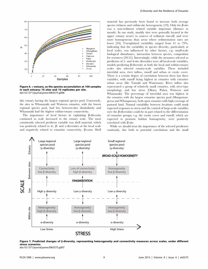
this estuary having the largest regional species pool. Conversely,

the sites in Whananaki and Waiwera estuaries, with the lowest

regional species pool, had low between-sites dissimilarity and

Whananaki had the highest within-estuary connectivity.

The importance of local factors in explaining b-diversity

continued as scale increased to the estuary scale. The most

consistently selected predictor variable was shell material, which

was positively related to a-, b- and c-diversities at the local scale

and negatively related to estuarine connectivity, b-conn. Shell

material has previously been found to increase both average

species richness and within-site heterogeneity [19]. Only for b-site

was a non-sediment related variable important (distance to

mouth). In our study, muddy sites were generally located in the

upper estuary nearer to sources of sediment run-off, and were

more homogeneous than areas where sedimentation rates are

lower [34]. Unexplained variability ranged from 41 to 79%,

indicating that the variability in species diversity, particularly at

local scales, was influenced by other factors, e.g. small-scale

biological disturbance, interaction between species, competition

for resources [50,51]. Interestingly, while the measures selected as

predictors of c- and a-site diversities were all local-scale variables,

models predicting b-diversity at both the local and within-estuary

scales also selected estuary-scale variables. These included

intertidal area, river inflow, runoff and urban or exotic cover.

There is a certain degree of correlation between these last three

variables, with runoff being highest in estuaries with extensive

urban areas (like Tamaki and Waitemata). River inflow also

represented a group of relatively small estuaries, with river-type

morphology and low stress (Okura, Puhoi, Waiwera and

Whananaki). The percentage of intertidal area was highest in

the estuaries with the largest estuarine species pool (Mangeman-

geroa and Whangateau), both open estuaries with high coverage of

pastoral land. Natural variability between locations could mask

expected responses to stress and the control of large-scale variables

over the b-diversities could be in part related to the differentiation

of estuarine groups; e.g. the exotic cover and runoff, which are

expected to promote habitat homogeneity, were positively

correlated with b-site.

While we should treat the importance of the selected predictors

cautiously, due both to potential correlations and the small

Figure 6. c-estuary, as the species accumulation at 100 samplesin each estuary; 10 sites and 10 replicates per site.doi:10.1371/journal.pone.0065575.g006

Figure 7. Predicted changes of b-diversity, representing heterogeneity and connectivity measures across scales, under differentstress scenarios.doi:10.1371/journal.pone.0065575.g007



number of estuaries (9) sampled, the predictors did include those

representing both geomorphology and stress. At the within-estuary

scale, connectivity (b-conn) was negatively related to a potential

stressor (runoff), while at the site scale, heterogeneity (b-site) was

positively related to local variables related to habitat heterogeneity

(shell hash). The average within-site heterogeneity in species

richness (b-site) was similar across estuaries, but the estuary

heterogeneity in species composition (similarity between sites) was

lowest in Waiwera and site-connectivity to the regional species

pool (b-conn) was lowest in Mangemangeroa and Whangateau.

These patterns overlapped with the effects of estuarine morphol-

ogy and hydrodynamics on b-diversity and no strong evidence of

the predicted responses to the stress gradient were identified. In

systems subjected to low but cumulative disturbance, we should

expect increasing variability in local species richness across space

due to localised responses to disturbance [10,26]. An early

warning in our low stress scenarios would be high variability in

connectivity within an estuary (b-conn), with some sites starting to

lose connectivity across the estuary. The highest variation for b-

conn measures occurred in Mangemangeroa, Waitemata and

Waiwera. Waitemata had a high degree of urbanisation;

Mangemangeroa had been undergoing changes in land-use

associated with urbanisation; and Waiwera had considerable road

construction across the upper estuary. Another early warning

signal could be related to the heterogeneity in species composition

between sites across an estuary. The highest variation for between-

sites dissimilarity was again observed in Mangemangeroa and

Waitemata, and in the most urbanised estuary, Tamaki. Note that

Mangemangeroa had the lowest estuary connectivity (high b-conn)

and Waiwera had the highest within-estuary homogeneity (low

Jaccard dissimilarity).

Data from low stressed systems is needed to identify early

warning signals of increasing marine degradation [13]. Most

studies on early warning signals focus on temporal trends, for

which long-term data bases are necessary, or data needs to be

extracted from models [23,52,53]. Early signals based on data

analysed across spatial scales in low stress systems could thus prove

particularly useful tools to anticipating changes in benthic

ecosystems subjected to diffuse sources of cumulative stress. The

estuaries included in this study were subjected to low stress, where

impact responses related to heterogeneity and connectivity

measures were not strong. Results confirm the complexity of

natural systems, where responses to cumulative stress in terms of

shifts in heterogeneity and connectivity do not follow linear

patterns and should be placed within the wider context of diversity

estimates across scales (Fig. 7). However, our results suggested links

between predicted land-based stressors and b-diversity, as the

estuaries with larger urbanised areas in the catchment had

increased variability in b-diversity across the estuary. The

implications of this for management are important in the context

of spatial planning and maintaining the adaptive capacity of

estuarine ecosystems. While large-scale heterogeneity might still

sustain a large regional species pool in the studied systems, the

increased variability across some of the most stressed estuaries

implies that persisting cumulative impacts could trigger ecological

fragmentation across the estuary and consequent decrease of

resilience of ecological communities. While this study does not

suggest a single indicator of ecosystems to stress, it suggests that

combined b-diversity metrics are good candidates for early

warnings in low stressed systems to predict loss of resilience due

to community homogenisation and loss of ecological connectivity.

Supporting Information

Table S1 Summary of the diversity measures fromwithin-site to estuary spatial scales. a-site is the average

species richness at a site (mean 6 SD, n = 10 replicates); c-site is

the total species richness predicted from the accumulation of 10

replicates per site; b-site is the additive b-diversity at the within-site

scale (c-site - a-site); c-estuary is the total species richness predicted

from the accumulation of 10 replicates 610 sites in each estuary;

b-conn is the additive b-diversity at the within-estuary scale (c-

estuary - c-site); between-site Jaccard is the average similarity

between all pair of sites within the estuary.

(DOCX)

Acknowledgments

We thank Sarah Hailes, Carolyn Lundquist, Barry Greenfield and Kelly

May with help with the field work.

Author Contributions

Conceived and designed the experiments: SFT JEH. Performed the

experiments: SFT JEH. Analyzed the data: SdJ. Wrote the paper: SdJ SFT

JEH.

References

1. Thrush SF, Gray JS, Hewitt JE, Ugland K (2006) Predicting the effects of habitat

homogenization on marine biodiversity. Ecological Applications 16: 1636–1642.

2. de Juan S, Hewitt J (2011) Relative importance of local biotic and environmental

factors versus regional factors in driving macrobenthic species richness in

intertidal areas. Marine Ecology Progress Series 423: 117–129.

3. Koleff P, Gaston KJ, Lennon JJ (2003) Measuring beta diversity for presence-

absence data. Journal of Animal Ecology 72: 367–382.

4. Anderson M, Ellingsen K, McArdle BH (2006) Multivariate dispersion as a

measure of beta diversity. Ecology Letters 9: 683–693.

5. Ellingsen KE (2002) Soft-sediment benthic biodiversity on the continental shelf

in relation to environmental variability. Marine Ecology Progress Series 232:

15–27.

6. Thrush SF, Hewitt JE, Cummings VJ, Norkko A, Chiantore M (2010) beta-

diversity and species accumulation in Antarctic coastal benthos: influence of

habitat, distance and productivity on ecological connectivity. PloS ONE 5:

e11899.

7. Thrush SF, Hewitt JE, Lohrer AM, Chiaroni LD (2013) When small changes

matter: the role of cross-scale interactions between habitat and ecological

connectivity in recovery. Ecological Applications 23: 226–238.

8. Scheffer M, Carpenter SR, Lenton TM, Bascompte J, Brock W, et al. (2012)

Anticipating Critical Transitions. Science 338: 344–348.

9. Thrush SF, Hewitt JE, Lohrer A (2012) Interaction networks in coastal soft-

sediments highlight the potential for change in ecological resilience. Ecological

Applications 22: 1213–1223.

10. Hewitt J, Thrush S, Lohrer A, Townsend M (2010) A latent threat to

biodiversity: consequences of small-scale heterogeneity loss. Conservation

Biology 19: 1315–1323.

11. Gering JC, Crist TO, Veech JA (2003) Additive partitioning of species diversity

across multiple spatial scales: implications for regional conservation of

biodiversity. Conservation Biology 17: 488–499.

12. Shackell NL, Fisher JD, Frank KT, Lawton P (2012) Spatial scale of similarity as

an indicator of metacommunity stability in exploited marine systems. Ecological

Applications 22: 336–348.

13. Halpern BS, Walbridge S, Selkoe KA, Kappel C V., Micheli F, et al. (2008) A

global map of human impact on marine ecosystems. Science 319: 948–952.

14. Bevilacqua S, Plicanti A, Sandulli R, Terlizzi A (2012) Measuring more of b-

diversity: Quantifying patterns of variation in assemblage heterogeneity. An

insight from marine benthic assemblages. Ecological Indicators 18: 140–148.

15. Cottenie K, De Meester L (2004) Metacommunity structure: synergy of biotic

interactions as selective agents and dispersal as fuel. Ecology 85: 114–119.

16. Shurin JB, Allen EG (2001) Effects of competition, predation, and dispersal on

species richness at local and regional scales. The American Naturalist 158: 624–

637.

17. Soininen J, Mcdonald R, Hillebrand H (2007) The distance decay of similarity in

ecological communities. Ecography 30: 3–12.

18. Keil P, Schweiger O, Kuhn I, Kunin W, Kuussaari M, et al. (2012) Patterns of

beta diversity in Europe: the role of climate, land cover and distance across

scales. Journal of Biogeography 39: 1473–1486.



19. Hewitt J, Thrush SF, Halliday J, Duffy C (2005) The importance of small-scale

habitat structure for maintaining beta diversity. Ecology 86: 1619–1626.

20. Koch E., Barbier EB, Silliman BR, Reed DJ, Perillo GM, et al. (2009) Non-

linearity in ecosystem services: temporal and spatial variability in coastal

protection. Frontiers in Ecology and the Environment 7: 29–37.

21. Scheffer M, Bascompte J, Brock W, Brovkin V, Carpenter S, et al. (2009) Early-

warning signals for critical transitions. Nature 461: 53–59.

22. Carpenter SR, Cole JJ, Pace ML, Batt R, Brock W, et al. (2011) Early warnings

of regime shifts: a whole-ecosystem experiment. Science 332: 1079–1082.

23. Lindegren M, Dakos V, Groger JP, Gardmark A, Kornilovs G, et al. (2012)

Early detection of ecosystem regime shifts: a multiple method evaluation for

management application. PloS ONE 7: e38410.

24. Carpenter S, Walker B, Anderies JM, Abel N (2001) From metaphor to

measurement: Resilience of what to what? Ecosystems 4: 765–781.

25. Fujita R, Moxley JH, DeBey H, Van Leuvan T, Leumer A, et al. (2013)

Managing for a resilient ocean. Marine Policy 38: 538–544.

26. Guttal V, Jayaprakash C (2009) Spatial variance and spatial skewness: leading

indicators of regime shifts in spatial ecological systems. Theoretical Ecology 2: 3–

12.

27. Dakos V, Nes EH, Donangelo R, Fort H, Scheffer M (2009) Spatial correlation

as leading indicator of catastrophic shifts. Theoretical Ecology 3: 163–174.

28. Brock WA, Carpenter SR (2010) Interacting regime shifts in ecosystems:

implication for early warnings. Ecological Monographs 80: 353–367.

29. Hewitt JE, Thrush SF (2010) Empirical evidence of an approaching alternate

state produced by intrinsic community dynamics, climatic variability and

management actions. Marine Ecology Progress Series 413: 267–276.

30. Thrush SF, Hewitt JE, Dayton PK, Coco G, Lohrer AM, et al. (2009)

Forecasting the limits of resilience?: integrating empirical research with theory.

Proceedings of the Royal Society 276: 3209–3217.

31. Thrush SF, Chiantore M, Asnagi V, Hewitt J, Fiorentino D, et al. (2011)

Habitat-diversity relationships in rocky shore algal turf infaunal communities.

Marine Ecology Progress Series 424: 119–132.

32. Lundquist C, Thrush S, Coco G, Hewitt J (2010) Interactions between

disturbance and dispersal reduce persistence thresholds in a benthic community.

Marine Ecology Progress Series 413: 217–228.

33. Edgar GJ, Barrett NS (2000) Effects of catchment activities on macrofaunal

assemblages in Tasmanian estuaries. Estuarine, Coastal and Shelf Science 50:

639–654.

34. Thrush SF, Hewitt JE, Cummings VJ, Ellis J, Hatton C, et al. (2004) Muddy

waters: elevating sediment input to coastal and estuarine habitats. Frontiers in

Ecology and the Environment 2: 299–306.

35. Hume T, Snelder T, Weatherhead M, Liefting R (2007) A controlling factor

approach to estuary classification. Ocean & Coastal Management 50: 905–929.

36. Bierschenk AM, Savage C, Townsend CR, Matthaei CD (2012) Intensity of land

use in the catchment influences ecosystem functioning along a freshwater-marinecontinuum. Ecosystems 15: 637–651.

37. Anderson MJ, Crist TO, Chase JM, Vellend M, Inouye BD, et al. (2011)

Navigating the multiple meanings of b diversity: a roadmap for the practicingecologist. Ecology letters 14: 19–28.

38. Ricotta C (2008) Computing additive beta-diversity from presence and absencescores: a critique and alternative parameters. Theoretical population biology 73:

244–249.

39. Loreau M (2000) Are communities saturated? On the relationship betweenalpha, beta and gamma diversity. Ecology Letters 3: 73–76.

40. Lande R (1996) Statistics and partitioning of species diverisity, and similarityamong multiple communities. Oikos 76: 5–13.

41. Jost L (2007) Partitioning diversity into independent alpha and beta components.Ecology 88: 2427–2439.

42. Colwell RK, Mao CX, Chang J (2004) Interpolating, extrapolating, and

comparing incidence-based species accumulation curves. Ecology 85: 2717–2727.

43. Hastie TJ, Tibshirani R (1990) Generalized Additive Models. Chapman andHall. London.

44. Breiman L (2001) Random Forests. Machine Learning 45: 5–32.

45. Wood SN, Augustin NH (2002) GAMs with integrated model selection usingpenalized regression splines and applications to environmental modelling.

Ecological Modelling 157: 157–177.46. Clarke KR, Warwick RM (1994) Changes in marine communities: an approach

to statistical analysis and interpretation. Natural Environment ResearchCouncil, Plymouth, UK.

47. Colwell R (2006) EstimateS: Biodiversity estimation. Available: http: //

viceroy.eeb.uconn.edu/EstimateS. Accessed 10 February 2012.48. Freestone AL, Inouye BD (2006) Dispersal limitation and environmental

heterogeneity shape scale-dependent diversity patterns in plant communities.Ecology 87: 2425–2432.

49. Thrush SF, Halliday J, Hewitt JE, Lohrer AM (2008) The effects of habitat loss,

fragmentation, and community homogenization on resilience in estuaries.Ecological Applications 18: 12–21.

50. Bruno JF, Stachowicz JJ, Bertness MD (2003) Inclusion of facilitation intoecological theory. Trends in Ecology and Evolution 18: 119–125.

51. Levin SA, Paine RT (1974) Disturbance, patch formation, and communitystructure. Proceedings of the National Academy of Sciences 71: 2744–2747.

52. Dakos V, Carpenter SR, Brock WA, Ellison AM, Guttal V, et al. (2012) Methods

for detecting early warnings of critical transitions in time series illustrated usingsimulated ecological data. PloS ONE 7: e41010.

53. Scheffer M, Carpenter S, Foley JA, Folke C, Walker B (2001) Catastrophic shiftsin ecosystems. Nature 413: 591–596.



Documents

Counting on b-Diversity to Safeguard the Resilience of Estuaries