COUNTING POINTS ON ELLIPTIC CURVES OVER F2n, then it is

mathematics of computationvolume 60, number 201january 1993, pages 407-420

COUNTING POINTS ON ELLIPTIC CURVES OVER F2n,

ALFRED J. MENEZES, SCOTT A. VANSTONE, AND ROBERT J. ZUCCHERATO

Abstract. In this paper we present an implementation of Schoofs algorithm

for computing the number of i"2m-P°mts °f an elliptic curve that is defined over

the finite field F2m . We have implemented some heuristic improvements, and

give running times for various problem instances.

1. INTRODUCTION

The use of elliptic curves in public key cryptography was first proposed by

N. Koblitz [5] and V. Miller [10]. Since then, a significant amount of research

has been done on the implementation of practical and secure cryptosystems

based on elliptic curves. For a secure system, one should select a curve E over

a finite field Fq such that the order, #E(Fq), of the group of points has a large

prime divisor. There are some families of curves whose orders are trivial to

compute (see [7] for some examples). However, if a random curve is chosen,

then it is necessary to have an efficient algorithm for computing its order.

In 1985, Schoof [ 13] gave a polynomial-time algorithm for computing #E(Fq).

The algorithm has a running time of 0(log q) bit operations, and is rathercumbersome in practice. In [3] the authors combined Schoofs algorithm with

Shanks' baby-step giant-step algorithm, and were able to compute orders of

curves over Fp , where p is a 27-decimal-digit prime. The algorithm took 4.5hours on a SUN-1 SPARC station.

The work mentioned above was all described for the case q odd. From a

practical point of view, however, curves over fields of characteristic 2 are more

attractive, since the arithmetic in F2m is easier to implement in hardware thanthe arithmetic in Fq, q odd. In [6] Koblitz adapted Schoofs algorithm to

curves over F2m and studied the implementation and security of a random-

curve cryptosystem. Special emphasis was placed on the underlying field F2m.

Recently, Agnew, Mullin, and Vanstone [1] have developed a VLSI device to

perform arithmetic in F2,ss and to perform computations on a random elliptic

curve over this field. Consequently, it is of interest to determine the order of

random curves over F2\s$.

We have implemented Schoofs algorithm for counting the points on an ar-

bitrary curve over F2m , and have employed some heuristics to improve the

actual running time. We are able to compute #E(F2m) for m = 155 (and so

#£(/>) « 1047) in about 61 hours on a SUN-2 SPARC station.

Received by the editor February 20, 1992.

1991 Mathematics Subject Classification. Primary 11Y40, 11T71; Secondary 94A60, 68P25,11Y16.

©1993 American Mathematical Society

0025-5718/93 $1.00 + 5.25 per page

407

License or copyright restrictions may apply to redistribution; see http://www.ams.org/journal-terms-of-use

408 A. J. MENEZES, S. A. VANSTONE, AND R. J. ZUCCHERATO

The remainder of the paper is organized as follows. In §2, we mention the

relevant properties of elliptic curves over finite fields of characteristic 2. In §3,

we outline Schoofs algorithm, and in §4 we present our heuristics for improving

Schoofs algorithm. Section 5 discusses details of our implementation, and gives

some running times for various problem instances. Finally, in §6, we survey the

latest research on the problem of counting points on an elliptic curve.

2. Elliptic curves in characteristic 2

Let q = 2m , and let K = Fq be the finite field of q elements. We denote the

algebraic closure of K by K. If S is a field or an additive group, then S* will

denote the nonzero elements of S. There are two types of elliptic curves over

K . A supersingular curve E over K is the set of solutions (x, y) £ K x K to

an equation of the form

(1) y2 + a-sy = x3 + a4x + a6,

with 03, a4, Û6 € K, ú¡3 t¿ 0, together with the "point at infinity" denoted^.

A nonsupersingular curve E over K is the set of solutions (x, y) £ K x K to

an equation of the form

(2) y2 + xy = x3 + a2x2 + a6,

with a2, a¿ £ K, a&^0, together with the point tf.If L is any field with K C L ç K, then let E(L) denote the set of points

in E both of whose coordinates lie in L, together with the point ¿f.

There are precisely three isomorphism classes of supersingular elliptic curves

over K if m is odd, and seven classes if m is even. The number of points

on a curve in each class is known [9]. Given a supersingular curve (1), we can

then compute #E(K) by determining the isomorphism class that E belongs to.

For the remainder of the paper we will thus be interested in computing #E(K),where £ is a nonsupersingular elliptic curve.

There are 2q - 2 isomorphism classes of nonsupersingular curves over K.

A set of representatives of these classes is

[y2 + xy = x3 + a2x2 + a6\a6 £ K*, a2 £ {0, y}},

where y £ K is a fixed element of trace 1. If E and E are the curves y2+xy =

x3 + a¿ and y2 + xy = x3 + yx2 + a¿, respectively, then it is easily verified that

#E(K) + #E(K) = 2q + 2 . Henceforth we will always assume that the equation

for E is of the form

(3) y2 + xy = x3 + a6, a6 £ K*.

It is well known that E has the structure of an abelian group, with the point

cf serving as its identity element. The rules for adding points on the curve (3)

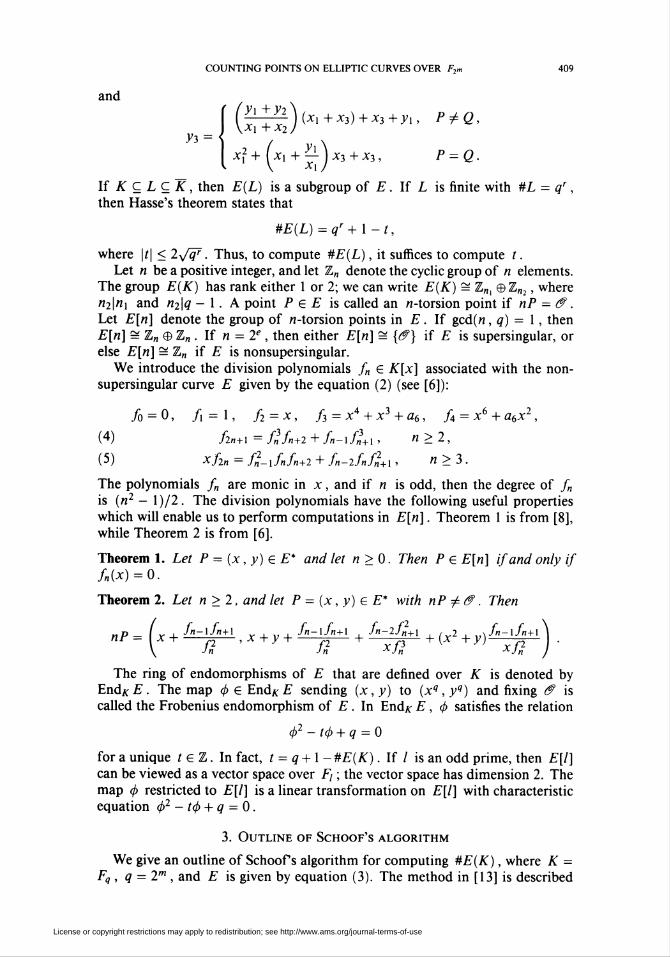
are the following. Let P = (xx, yx) £ E* ; then -P = (x\, Vi +Xx). Notice that

P and -P have the same x-coordinates. If Q = (x2, y2) £ E* and Q ¿ -P,

then P + Q = (x-$, y?,), where

— ) \xl + x2f Xx +X2

^+x2, P = Q,xi


COUNTING POINTS ON ELLIPTIC CURVES OVER F2m 409

and

V3

r (y\ +y2\

\Xi+X2)(x1+x3) + x3+yi, P^Q,

Cx + x" '

If K ç L Ç K, then E(L) is a subgroup of E. If L is finite with #L = qr,then Hasse's theorem states that

#E(L) = qr + X-t,

where |i| < 2v/tf7. Thus, to compute #E(L), it suffices to compute t.

Let « be a positive integer, and let Z„ denote the cyclic group of n elements.

The group E(K) has rank either 1 or 2; we can write E(K) = Z„, ©Z„2, where

n2\nx and «2k - 1. A point P £ E is called an «-torsion point if nP = &.Let E[n] denote the group of n-torsion points in E. If gcd(«, q) = X , then

E[n] =■ Z„ 9 Z„ . If « = 2e , then either £[«] S {^} if £ is supersingular, or

else E[n] = Z„ if E is nonsupersingular.

We introduce the division polynomials /„ £ K[x] associated with the non-supersingular curve E given by the equation (2) (see [6]):

fo = 0, fx = X, f2=x, ft = x4 + x3 + a6, f4 = x6 + a6x2,

(4) /2fl+l = fifn+2 + fn-lflx , « > 2,

(5) Xf2n = f„-xfnfn+2 + fn-2fnf„+l > « > 3.

The polynomials /„ are monic in x, and if n is odd, then the degree of /„

is (n2 — X)/2. The division polynomials have the following useful properties

which will enable us to perform computations in E[n]. Theorem 1 is from [8],

while Theorem 2 is from [6].

Theorem 1. Let P = (x, y) £ E* and let n>0. Then P £ E[n] if and only if

fn(x) = 0.

Theorem 2. Let n > 2, and let P = (x, y) e E* with nP / tf. Then

nP=(x+ /n-'f"+1 , x + y + fn-\{n+x + fn-2$+x + (x2 + y)f"-xfn+x \fi ' '" ft Xfn3 V y> Xf2 )■

The ring of endomorphisms of E that are defined over K is denoted by

EndxE. The map <f> £ End*;/? sending (x,y) to (xq ,yq) and fixing & is

called the Frobenius endomorphism of E. In End*; E, <f> satisfies the relation

(j)2 - t<p + q = 0

for a unique t £ Z. In fact, t = q + X - #E(K). If / is an odd prime, then E[l]can be viewed as a vector space over F¡ ; the vector space has dimension 2. The

map <p restricted to E[l] is a linear transformation on E[l] with characteristic

equation <f>2 - t<p + q = 0.

3. Outline of Schoof's algorithm

We give an outline of Schoof s algorithm for computing #E(K), where K =

Fq , q = 2m , and E is given by equation (3). The method in [13] is described


410 A. J. MENEZES, s. a. vanstone, and r. j. zuccherato

for fields of odd characteristic. More details for the case q even will be given

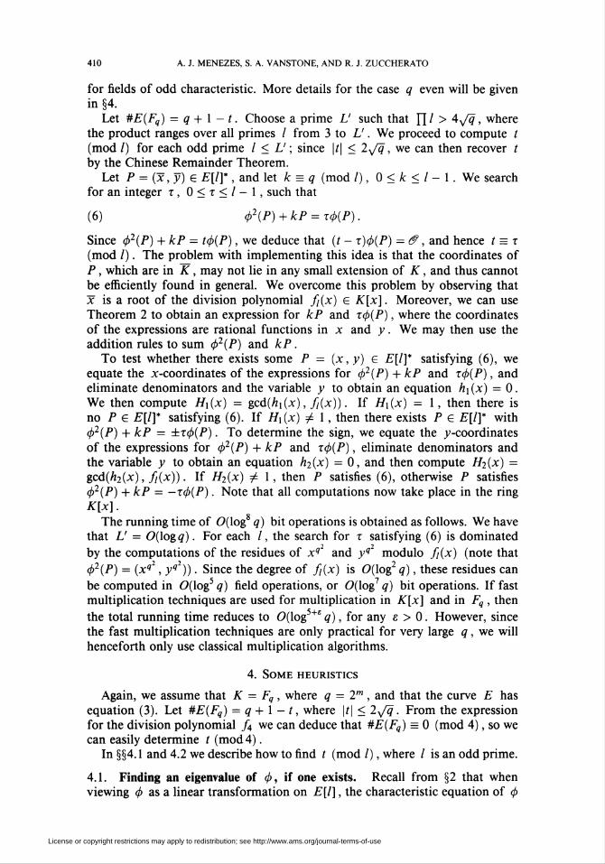
in §4.Let #E(Fq) = q + X - t. Choose a prime L' such that Y\l > 4^/q, where

the product ranges over all primes / from 3 to L'. We proceed to compute t

(mod /) for each odd prime /</_/; since \t\ < 2^/q, we can then recover t

by the Chinese Remainder Theorem.

Let P = (x, y) £ E[l]*, and let k = q (mod /), 0 < k < I - X. We searchfor an integer x, 0 < x < I - 1, such that

(6) <t>2(P) + kP = X<f>(P) .

Since 4>2(P) + kP = t<f>(P), we deduce that (t - x)tp(P) = tf, and hence t = x(mod /). The problem with implementing this idea is that the coordinates of

P, which are in K, may not lie in any small extension of K, and thus cannot

be efficiently found in general. We overcome this problem by observing that

x is a root of the division polynomial f(x) e K[x]. Moreover, we can use

Theorem 2 to obtain an expression for kP and x<p(P), where the coordinates

of the expressions are rational functions in x and y. We may then use the

addition rules to sum <p2(P) and kP.To test whether there exists some P = (x, y) £ E[l]* satisfying (6), we

equate the x-coordinates of the expressions for 4>2(P) + kP and x4>(P), and

eliminate denominators and the variable y to obtain an equation «i(x) = 0.

We then compute Hx(x) = gcd(«i(x), f(x)). If Hx(x) = X, then there is

no P £ E[l]* satisfying (6). If Hx(x) ¿ X, then there exists P £ E[l]* with4>2(P) + kP = ±x(j)(P). To determine the sign, we equate the y-coordinates

of the expressions for <j>2(P) + kP and x<f>(P), eliminate denominators and

the variable y to obtain an equation h2(x) = 0, and then compute H2(x) =

gcd(h2(x), fi(x)). If H2(x) ^ 1, then P satisfies (6), otherwise P satisfies

4>2(P) + kP = -x<t>(P). Note that all computations now take place in the ring

K[x].

The running time of 0(log8 q) bit operations is obtained as follows. We have

that L' = 0(Xogq). For each /, the search for t satisfying (6) is dominated

by the computations of the residues of xq and yq modulo f(x) (note that

4>2(P) = (xq , yq )). Since the degree of f(x) is 0(log2 q), these residues can

be computed in 0(log5 q) field operations, or 0(log7 q) bit operations. If fast

multiplication techniques are used for multiplication in K[x] and in Fq , then

the total running time reduces to 0(log5+£ q), for any e > 0. However, since

the fast multiplication techniques are only practical for very large q, we will

henceforth only use classical multiplication algorithms.

4. Some heuristics

Again, we assume that K = Fq , where q = 2m , and that the curve E has

equation (3). Let #E(Fq) = q + X - t, where |/| < 2^/q. From the expression

for the division polynomial f4 we can deduce that #E(Fq) = 0 (mod 4), so we

can easily determine t (mod 4).

In §§4.1 and 4.2 we describe how to find t (mod /), where / is an odd prime.

4.1. Finding an eigenvalue of <p, if one exists. Recall from §2 that when

viewing 0 as a linear transformation on E[l], the characteristic equation of (j)


counting points on elliptic curves over F2 411

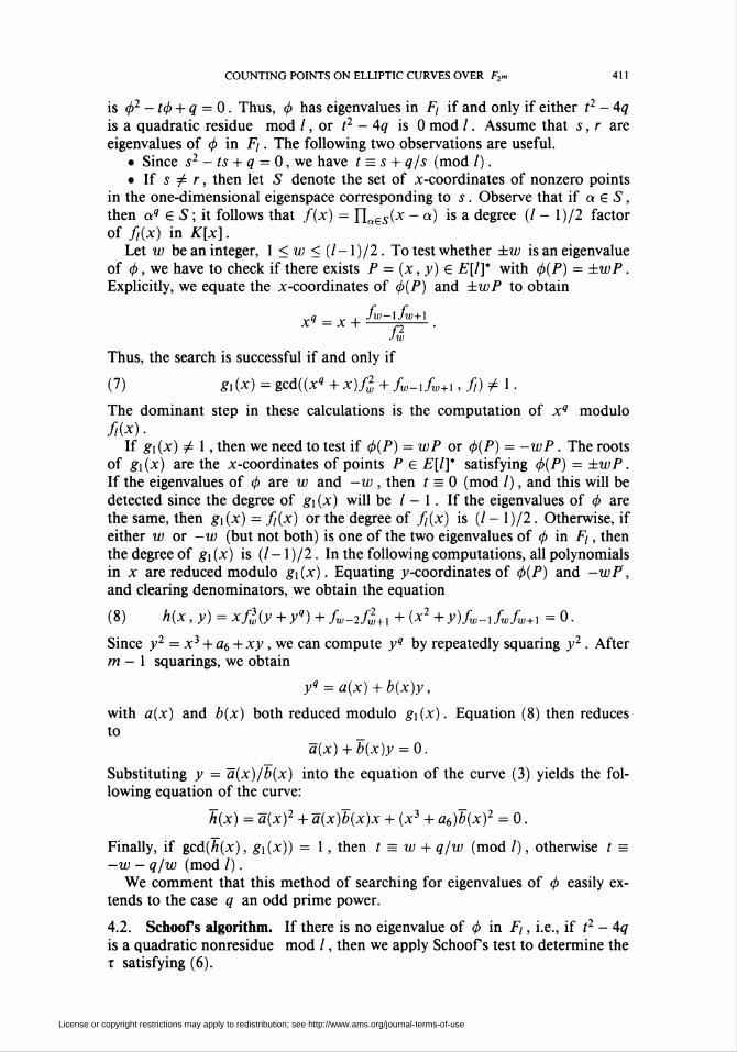
is 4>2 - t<j) + q = 0. Thus, <f> has eigenvalues in F¡ if and only if either t2 - 4qis a quadratic residue mod /, or t2 - 4q is 0 mod /. Assume that s, r are

eigenvalues of <j> in F¡. The following two observations are useful.

• Since s2 - ts + q = 0, we have t = s + q/s (mod /).

• If 5 t¿ r, then let S denote the set of x-coordinates of nonzero pointsin the one-dimensional eigenspace corresponding to s. Observe that if a £ S,

then aq £ S ; it follows that f(x) = Y\aeS(x -a) is a degree (/ - l)/2 factor

of fi(x) in K[x].Let w be an integer, X <w < (l-X)/2. To test whether ±w is an eigenvalue

of (¡>, we have to check if there exists P = (x, y) £ E[l]* with <p(P) = ±wP.

Explicitly, we equate the x-coordinates of <f>(P) and ±wP to obtain

q _ , Jw-lJw+l

X ~ A "1~ f2Jw

Thus, the search is successful if and only if

(7) gx(x) = gcd((x« + x)fl + fw-xfw+x ,f,)¿X.

The dominant step in these calculations is the computation of xq modulo

//(*)■If gx(x) t¿ 1, then we need to test if 4>(P) = wP or <¡>(P) = -wP. The roots

of gx(x) are the x-coordinates of points P £ E[l]* satisfying 4>(P) = ±wP.

If the eigenvalues of 0 are w and -w , then t = 0 (mod /), and this will be

detected since the degree of gi (x) will be / - 1. If the eigenvalues of <j> are

the same, then g\(x) = f(x) or the degree of f(x) is (/ - l)/2. Otherwise, ifeither w or -w (but not both) is one of the two eigenvalues of q> in F¡, then

the degree of gx(x) is (/-1)/2. In the following computations, all polynomials

in x are reduced modulo gx(x). Equating y-coordinates of <f>(P) and -wP,and clearing denominators, we obtain the equation

(8) h(x,y) = xf3(y + yq)+fw-2f¿+l + (x2 +y)fw-xfwfw+i =0.

Since y2 = x3 + a6 + xy, we can compute yq by repeatedly squaring y2. After

m - X squarings, we obtain

yq = a(x) + b(x)y,

with a(x) and b(x) both reduced modulo gx(x). Equation (8) then reduces

toa(x) + b(x)y = 0.

Substituting y = a~(x)/b(x) into the equation of the curve (3) yields the fol-

lowing equation of the curve:

h(x) = d~(x)2 + a~(x)b(x)x + (x3 + a6)b(x)2 = 0.

Finally, if gcd(/z(x), gx(x)) = 1, then t = w + q/w (mod /), otherwise / =

-w - q/w (mod /).We comment that this method of searching for eigenvalues of <f> easily ex-

tends to the case q an odd prime power.

4.2. Schoof s algorithm. If there is no eigenvalue of </> in F¡, i.e., if t2 - 4q

is a quadratic nonresidue mod /, then we apply Schoof s test to determine thex satisfying (6).


412 A. J. menezes, s. a. vanstone, and r. j. zuccherato

We first check if there is a P = (x, y) £ E[l]* with 4>2(P) = ±kP, where kis q modulo /. This is the case if and only if

gcd((xq2 + x)f2 + fk_xfk+l, fi) ¿ X.

Observe that if t = 0 (mod /), then <f>2(P) = -kP. Now, if 4>2(P) = kP, then<j>(P) = (2k/t)P, whence (p has an eigenvalue in F¡. But t2 -4q is a quadratic

nonresidue mod /, so we conclude that 4>2(P) = -kP. Thus, t(j)(P) = <f and

t = 0 (mod /).Assume now that there is no P £ E[l]* with 4>2(P) = ±kP. In order to

determine t (mod /), we check for each x, X < x < I - 1, if there exists

P £ E[l]* satisfying (6). Since 4>2(P) / ±kP, we can use the rule for adding

distinct points to compute an expression for 4>2(P) + kP. Explicitly, let (P)x

denote the x-coordinate of point P. Then for k > 2

(9) (±x<t>(P))x = xq + fr-xfr+x

ft"

(<t>2(P) + kP)x = xql + x + fk~xJ2k+x +X2 + X,h

(yql + y + x)xf3 + fk-2ft+x +(x2 + x + y)(fk-Xfkfk+x)

and

where

(10) X =xf3(x + xq2) + xfk_xfkfk+x

Similar equations can be obtained for the case k = X. Equate the x-coordinates

of 4>2(P) + kP and ±x<f>(P), and eliminate denominators and the variable y ,

to get an identity «3(x) = 0. Then there exists a P £ E[l]* with tj>2(P) + kP =

±xcj)(P) if and only if h4(x) = gcd(«3(x), f(x)) / 1. This is repeated foreach x, 1 < x < (I - l)/2, for which x2 - 4q is a nonresidue (mod/). If the

gcd is nontrivial, then we can determine the correct sign by first equating the

y-coordinates of <f>2(P) + kP and x<t>(P). Explicitly, for x > 2,

fQ fQ fq f2q fq fq(11) (x<p(P))y = xq+yq + ^£±i + ¿lî±i + {x2q + y«)^|±!

7t XqJx XqJx

and(4>2(P) + kP)y = X(xqI + x3) + X3 + yql,

where X3 = (</>2(P) + kP)x and X is as in (10) (similar equations can be ob-

tained for the case x = 1 ). As was done above, we then proceed to eliminate

the denominator and the variable y to get an identity h5(x) = 0. Then, if

gcd(//(x), hs(x)) t¿ 1, we have t = x ; otherwise t = -x. The dominant step

in these calculations is the computation of xq and yq modulo f(x).

To determine / (mod /) in practice, one would first search for an eigenvalue

of 4> in F¡, and if this fails, then Schoof s algorithm is applied. The firstmethod is faster since it only requires the residue of xq modulo f(x), while

the second method requires the residues xq , xq ,yq, and yq modulo f¡(x).

Heuristically, for a random curve, we would expect <b to have an eigenvalue in

F¡ (i.e., t2-4q is a quadratic residue in F¡) for half of all /'s. Moreover, if <p

does have eigenvlaues in F¡, then in most cases the eigenvalues will be distinct,

and so the test if 4>(P) = wP or 4>(P) = -wP in (4.1) takes negligible time

(since deggï(x) = (/ - l)/2 or / - 1).



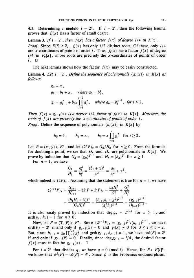
4.3. Determining t modulo I = 2C. If / = 2C, then the following lemma

proves that f(x) has a factor of small degree.

Lemma 3. If l = 2c, then f¡(x) has a factor f(x) of degree 1/4 in K[x].

Proof. Since E[l] =■ Z/, f(x) has only 1/2 distinct roots. Of these, only 1/4are x-coordinates of points of order /. Thus, f(x) has a factor f(x) of degree

1/4 in Fq[x], whose roots are precisely the x-coordinates of points of order

/. D

The next lemma shows how the factor f(x) may be easily constructed.

Lemma 4. Let I = 2C. Define the sequence of polynomials {g¡(x)} in K[x] as

follows:

go = x,

gx = bx + x, where a6 = b4,

i-1

gi = gf-X + biX Y[ gj, where a6 = bf , for i > 2.;=i

Then f(x) = gc-i(x) is a degree 1/4 factor of f(x) in K[x]. Moreover, the

roots of f(x) are precisely the x-coordinates of points of order I.

Proof. Define the sequence of polynomials {h¡(x)} in K[x] by

«o=l, «i = x, hi■■ = x Y\ gj for i > 2.j=i

Let P = (x, y) e E*, and let (2nP)x = Gn/Hn for « > 0. From the formula

for doubling a point, we see that G„ and Hn are polynomials in K[x]. We

prove by induction that Gn = (gn)2"+< and Hn = (h„)2" for n > X.

For n = X, we have

Gx_ _ g[ _ (¿1+X)4 _ 06 2

Hx h2 x2 x2+ '

which indeed is (2P)X . Assuming that the statement is true for n = i, we have

(2'+lP)x = |^ = (2'P + TP)X = ÜJ§- + %

(bxHi + Gi)4 ^ (bi+xhj + g2)2'+2 = (gi+x)2'+2

(GiHi)2 (g}hi)2M (hi+x)2M '

It is also easily proved by induction that degg„ = 2"~x for n > X, and

gcd(g„ , «„) = 1 for « >0.

Now, let P = (x, y)£E*. Since (2C~XP)X = (gc-xf /(hc-xf1, we haveord(P) = 2C if and only if &_i(x) = 0 and g¡(x) / 0 for 0 < / < c - 2.

But, since «c_i = goIT/I? SJ and S,cà{gc-i, hc-i) = 1, we have ord(P) = 2C

if and only if gc-i(x) = 0. Finally, since deggc_i = 1/4, the desired factor

f(x) must in fact be gc-x(x). D

For I = 2C that divides q , we have q = 0 (mod /). Hence, for P £ E[l]*,we know that </>2(P) — xq)(P) = (f. Since 4> is the Frobenius endomorphism,



4>(P) t¿ tf for P j^cf. Therefore, <p(P) -xP = <f and x is an eigenvalue of <f>

in Z/.Since we know that #E(Fq) = 0 (mod 4), we have that t = 1 (mod 4) and

t = 1 (mod 4). This gives us only two choices for x modulo 8. We can easily

obtain this eigenvalue using a factor of f%(x) obtained as above, and using our

heuristic for finding eigenvalues. This procedure can then similarly be applied

to finding eigenvalues for / = 16, 32, 64, ... . The method is efficient for /

being a small power of 2, since the polynomial arithmetic is performed modulo

a degree 1/4 factor of f(x).

4.4. Baby-step giant-step algorithm. The calculation of t modulo / using

Schoof s algorithm for small primes / is very simple. However, since deg(f(x))

= (I2 - X)/2, the calculation quickly becomes infeasible as the value of / in-

creases. In [3], the authors combined Schoof s algorithm with Shanks' baby-

step giant-step method. In this method, one first computes #E(Fq) modulo

L - lo • l\ ■ ■ ■ lr, where lx, ... , lr are small primes and /o is a small power of

2. We then use the baby-step giant-step algorithm to determine #E(Fq).

We describe Shanks' algorithm with suitable modifications for use with

Schoof s algorithm.

Step X. Choose a random point P in E(Fq) and set

k = min{Ä:'|Ä:' > \>JL • 4 . y/q~\, k' = 0 (mod L)}.

Step 2. Compute iP for i = ([q + X - 2Jq\ - #E(Fq)) (mod L) for 0 < / <k - 1 . If for some i we have iP = (f, then return to Step 1. Otherwise, store

i and the first 32 bits of the x-coordinate of iP in a table sorted by the entry

iP.

Step 3. Set Q = kP.

Step 4. Compute

Hj = [q + l-2y/q\P + jQ

for j = X ,2, ... , k/L and check (by a binary search) whether the first 32 bits

of the x-coordinate of Hj correspond to the first 32 bits of the x-coordinate

of iP for some /. If it does, we then check if H¡ = iP (by recalculating iP).

If we have only one pair (i, j) with Hj = iP, then

#E(Fq)=[q+X-2y/q\+kj-i,

and the algorithm terminates. If not, then return to Step 1.

We sketch the correctness and running time of the algorithm.

Since P £ E(Fq), then ord(P) divides #E(Fq). Thus, if there exists aunique integer r £ [q + X - 2^/q, q + X + 2^/q] such that rP = cf, then

r = #E(Fq) ; if not, then ord(P) < 4^/q . Either case is detected in Step 4. Thus

in Step 1 we hope that ord(P) > 4^/q .Recall that E(Fq) = Z„, © Z„2, where n\ \ n2 and n2 \ (q - X). For a

random elliptic curve, we would expect «i > «2 and so nx » 4^/q. Thus,

with very high probability, ord(P) > 4^/q. Since #E(Fq) > (y/q - X)2, wehave «1 > yfq - X . Moreover, since 4 | #E(Fq) and «2 is odd, we have

"1 > 2(v/<7- 1). If in fact nx < 4^/q , then there is no point in E(Fq) of order

greater than 4y/q. This will be detected since the algorithm will fail in Step 4



each time. If this happens, then we determine ord(P) and repeat the algorithm

until ord(P) > 2(y/q - 1). We then search for a point P' which has order > 3

in the quotient group E(Fq)/(P). For more details, consult [3].

The table in Step 2 has about S = 2qx/4/\[L entries, which are computed

with O(S) field operations. The table is then sorted using O(SXogS) com-

parisons. Computing Hj for j = X, 2, ... , k/L takes O(S) field operations,

while each binary search takes 0(XogS) comparisons. Thus the whole algorithm

takes 0(qx/4(Xogq)2/\/L) bit operations, and requires 0(qxl4(Xogq)/\fL) bits

of storage.

4.5. Checking results. Let #E(Fq) = q + X - t, where t is unknown, and

suppose that our algorithm outputs #E(Fq) = q + X - f. We may verify that

t = t' as follows.Let P be the point in the baby-step giant-step algorithm. Since the algorithm

terminated, we believe that ord(P) > 4^/q. We first verify that (q + X - t')P =

(f ; if this does not hold, then t ^ t'. We then proceed to factor q + X - t',

which is an easy task since q + X-t' < 1050 for the #'s we are concerned with.

Given the prime factorization of q + 1 - t', we can easily determine ord(P),

and we then check that ord(P) > 4^/q. Now, since (q + X - t)P = c? and

(q + X - t')P = £?, we deduce that (t - t')P = cf. Finally, since ord^) > 4^/qand \t - t'\ < 4yfq, we conclude that t = t'.

Of course, this check is only successful if «i > 4^/q, which, as pointed out

in §4.4, is true for most curves.

5. Implementation and results

The algorithm described in §4 was implemented in the C programming lan-guage on a SUN-2 SPARC station with 64 Mbytes of main memory. We make

some comments on our implementation.

(i) The elements of Fq = F2m were represented with respect to a normal

basis. This has the advantage that squaring a field element involves only a

cyclic shift of the vector representation. Explicitly, if yS is a normal basis

generator and a = ££ö' A,/?2', where X¡ £ F2, then a2 = Yô Vi A2' (withsubscripts reduced modulo m). For computational efficiency in multiplying

field elements, we use the special class of normal bases known as optimal normal

bases [11]; these bases only exist for certain values of m but are perhaps the

most important for practical purposes.

(ii) Let « = degyj(x). To compute gcd(,4(x), //(x)) for some A(x) £ K[x],

we first reduce ^(x) modulo f¡(x), and then compute the gcd of the resulting

polynomial with f(x). In order to compute xq (mod//(x)), which is needed,

for example, in (7), we precompute the residues x2j modulo f(x), for 0 < j <

n-X. Then xq (mod//(x)) is obtained by repeatedly squaring x . Explicitly,

x2'(modf,(x)) = (x2'~\modf,(x)))2(modf,(x))

(n-l \ n-l

YâjXi (modf(x)) = J2^(x2J(modf,(x))).;=0 / 7=0

The residues of xq ,yq, and yq modulo f(x) are obtained in a similarmanner.


416 A. J. menezes, s. a. vanstone, and r. j. zuccherato

(iii) In calculating (9) and (11), we need to compute fq (mod fi(x)), for

0 < x < (I - l)/2 + 1. Since we already know xq (mod^(x)), we can easily

compute y? (mod//(x)) recursively:

^=0(mod//(x)),

f? = X (modfi(x)),

fq=xq(modMx)),

fq = x4q + x3q + a6 (mod fi(x)),

fq = x6q + a6x2q (modfi(x)),

Í2i+i = fï9f?+2 + ff-ifUl (mod//(x)), i>2,

f2qi = s{x){fi2ïxfifï+2 + fi-2f?fM) (mod/,(*)), i>3,

where s(x) £ K[x] satisfies s(x)xq = X (modf¡(x)). Note that indeed

gcd(x« , f,(x)) = X

when / is odd, since the only points with x-coordinates equal to 0 have order

2.(iv) We chose /'s up to 31 in order to keep manageable the size of the space

searched in the baby-step giant-step part of the method. If more memory is

available, then the cases / = 29 and / = 31 may be excluded, at the expense

of an increase in the time for the baby-step giant-step part.

Using the method of §4.3, we also computed t modulo 64. If ( t modulo

64) < 31, then we compute t modulo 128 (for this we only need the division

polynomials f(x), 1 < i < 31, modulo the degree-32 factor of fxni*)) •Similarly, if ( t modulo 128) < 31, we compute / modulo 256. In this way we

may compute t modulo 1024.(v) In the baby-step giant-step algorithm we need to select points uniformly

at random from E(Fq). This is accomplished as follows. First pick a random

element x £ Fq . The probablity that x is the x-coordinate of some P £ E(Fq)

is roughly j ; this follows from Hasse's theorem. We then attempt to solve the

equation

y2 + xy = x3 + a6

for y . There is a solution if and only if there is a solution to y2+y = b, where

b = x_2(x3 + ad). Compute b, and let

m— 1 m—l

b=Y,°iß2' and y=Yjyiß2'-;=0 ¡=0

Thenm-\ m-l

y2+y = Y,(yi-i+y>)ß2' = Y,b'ß2'-;=0 !=0

Select y0 = 0 or y0 = 1 at random. Since y0 + yi = bx, this determines yx.

Similarly, y2, y3, ... , ym-\ are determined. Finally, if ym-X + y0 = b0 , then

(x, xy) is a random point in E(Fq). Otherwise, x is not the x-coordinate of

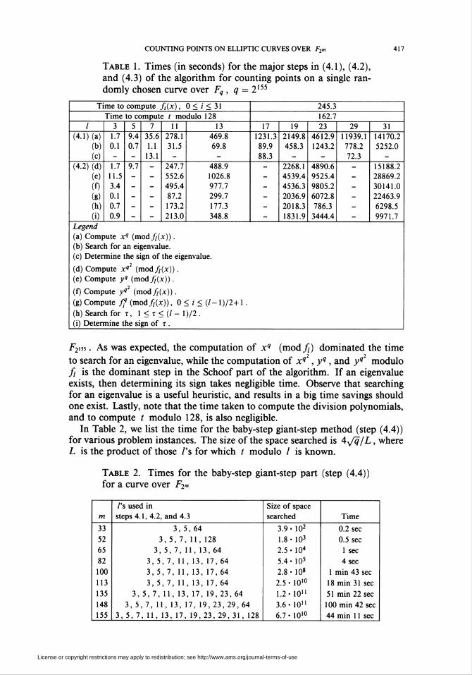
a point in E(Fq).In Table 1, we list the time taken for the major steps in (4.1), (4.2), and (4.3)

of our algorithm for counting points on a single randomly chosen curve over


COUNTING POINTS ON ELLIPTIC CURVES OVER F2 417

Table 1. Times (in seconds) for the major steps in (4.1), (4.2),

and (4.3) of the algorithm for counting points on a single ran-

domly chosen curve over Fq , q = 2155

Time to compute f(x) » 0 < i < 31 245.3

Time to compute t modulo 128 162.7

11 13 17 19 23 29 31

(4.1) (a)

(b)

(c)

1.7

0.19.4

0.735.61.1

13.1

278.1

31.5469.869.8

1231.389.988.3

2149.8458.3

4612.91243.2

11939.1778.2

72.3

14170.2

5252.0

(4.2) (d)(e)

(0(g)(h)

(i)

1.711.53.40.1

0.70.9

9.7 247.7

552.6495.487.2173.2213.0

488.91026.8977.7299.7177.3348.8

2268.14539.4

4536.32036.9

2018.31831.9

4890.69525.49805.26072.8786.3

3444.4

15188.2

28869.230141.022463.96298.59971.7

Legend

(a) Compute xq (moáf¡(x)).

(b) Search for an eigenvalue.

(c) Determine the sign of the eigenvalue.

(d) Compute xq (mod/;(x)).

(e) Compute yq (mod//(x)).

(f) Compute yql (mod/,(*)).

(g) Compute ff (mod/,(*)), 0 < i < (/-(h) Search for t , 1 < x < (I - l)/2.(i) Determine the sign of t .

0/2+1

F2i5s. As was expected, the computation of xq (mod.//) dominated the time2 2

to search for an eigenvalue, while the computation of xq , yq , and yq modulo

fi is the dominant step in the Schoof part of the algorithm. If an eigenvalueexists, then determining its sign takes negligible time. Observe that searching

for an eigenvalue is a useful heuristic, and results in a big time savings should

one exist. Lastly, note that the time taken to compute the division polynomials,

and to compute t modulo 128, is also negligible.

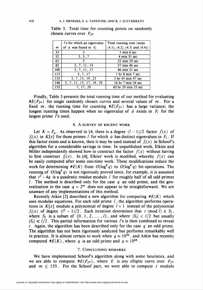
In Table 2, we list the time for the baby-step giant-step method (step (4.4))for various problem instances. The size of the space searched is 4^/q/L, whereL is the product of those /'s for which t modulo / is known.

Table 2. Times for the baby-step giant-step part (step (4.4))

for a curve over F2m

/'s used in

steps 4.1, 4.2, and 4.3

Size of space

searched Time

33

52

65

82

100

113

135

148

155

3, 5,64

3, 5, 7, 11, 128

3, 5, 7, 11, 13, 64

3, 5, 7, 11, 13, 17, 64

3, 5, 7, 11, 13, 17,64

3, 5, 7, 11, 13, 17,64

3, 5, 7, 11, 13, 17, 19,23, 64

3, 5, 7, 11, 13, 17, 19,23,29,64

3, 5, 7, 11, 13, 17, 19,23, 29, 31, 128

3.91.8

2.5

5.4

2.8

2.5'

1.2

3.66.7>

■102

103■ 104

• 105

•108

1010

10"

10"

1010

0.2 sec

0.5 sec

1 sec

4 sec

1 min 43 sec

18 min 31 sec

51 min 22 sec

100 min 42 sec

44 min 11 sec



Table 3. Total time for counting points on randomly

chosen curves over F2m

33

52

65

82

100

113

135

148155

/'s for which an eigenvalue

of <j> was found in F¡

3, 5, 7

5

3, 7, 11, 135, 7, 11, 17

3,7, 173, 7, 13, 19,23

5, 7, 11, 13, 17, 19, 297, 17,29

Total running time (steps

(4.1), (4.2), (4.3) and (4.4))

1 min 6 sec

4 min 51 sec

22 min 29 sec

57 min 46 sec

46 min 21 sec

1 hr 8 min 7 sec

5 hr 43 min 47 sec

16 hr 7 min 26 sec

60 hr 29 min 33 sec

Finally, Table 3 presents the total running time of our method for evaluating

#E(F2m) for single randomly chosen curves and several values of m. For a

fixed m, the running time for counting #E(F2m) has a large variance; the

longest running times happen when no eigenvalue of 0 exists in F¡ for the

largest prime /'s used.

6. A SURVEY OF RECENT WORK

Let K = Fq . As observed in §4, there is a degree (/ - l)/2 factor f(x) of

fi(x) in K[x] for those primes / for which (¡> has distinct eigenvalues in F¡. If

this factor exists and is known, then it may be used instead of f(x) in Schoof s

algorithm for a considerable savings in time. In unpublished work, Elkies and

Miller independently showed how to construct the factor f(x) without having

to first construct f(x). In [4], Elkies' work is modified, whereby f(x) can

be easily computed after some one-time work. These modifications reduce the

work for determining #E(K) from 0(log8 q) to 0(log6 q) bit operations. The

running of (7(log6 q) is not rigorously proved since, for example, it is assumed

that t2 -4q is a quadratic residue modulo / for roughly half of all odd primes

/. The method is described only for the case q an odd prime, and the gen-

eralization to the case q = 2m does not appear to be straightforward. We are

unaware of any implementations of this method.Recently Atkin [2] described a new algorithm for computing #E(K) which

uses modular equations. For each odd prime /, the algorithm performs opera-

tions in K[x] modulo a polynomial of degree / + 1 instead of the polynomial

f(x) of degree (I2 - X)/2. Each iteration determines that t (modi) £ S¡,

where S¡ is a subset of {0, 1,2,...,/}, and where \S¡\ < 1/2 but usually

\Si\ <C 1/2. This partial information for various /'s is then combined to reveal

t. Again, the algorithm has been described only for the case q an odd prime.

The algorithm has not been rigorously analyzed but performs remarkably well

in practice. It is almost certain to work when q ¡=s 1050 , and Atkin has recently

computed #E(K), where q is an odd prime and q « 1068.

7. Concluding remarks

We have implemented Schoof s algorithm along with some heuristics, and

we are able to compute #E(F2m), where E is any elliptic curve over F2m

and m < 155. For the Schoof part, we were able to compute t modulo



/ for / = 3, 5, 7, 11, 13, 17, 19,23, 29, 31, and 64 (and sometimes / =128,256, 512,1024).

Computing #E(F2iss) takes roughly 61 hours on a SUN-2 SPARC station.

(The algorithm takes 61 hours or less provided that </> has an eigenvalue in

either F2g or F3l . Heuristically, one would expect this to occur about 75%

of the time for random curves.) On the SPARC station, we can multiply field

elements in F2m at the rate of 900 multiplications per second. There exists a

special purpose chip which does the field arithmetic in F2¡ss and can perform

250,000 multiplications per second [1]. Since roughly 90% of all time of the

algorithm is spent in multiplying field elements in F2m, the use of this chip

should reduce the time for computing #E(F2i>}) to about 6 hours.

Possible improvements which we did not implement are the computation of

t modulo 27, and using Pollard's Lambda method for catching kangaroos [12]

instead of the baby-step giant-step algorithm. Pollard's method has the same

expected running time as the latter method, but requires very little storage.

Finally, as pointed out by Atkin [2], we mention that the information ob-

tained from Schoof s algorithm and the heuristics presented here can be com-

bined with the information from Atkin's method to compute #E(F2m) for even

larger values of m .

Acknowledgment

We would like to thank an anonymous referee and A. Atkin for their careful

reading of this paper, and for suggesting some useful improvements.

Bibliography

1. G. Agnew, R. Mullin, and S. Vanstone, An implementation of elliptic curve cryptosystems

over F2i55 , preprint.

2. A. Atkin, The number of points on an elliptic curve modulo a prime, unpublished manuscript,

1991.

3. J. Buchmann and V. Müller, Computing the number of points of elliptic curves over fi-nite fields, presented at International Symposium on Symbolic and Algebraic Computation,

Bonn, July 1991.

4. L. Charlap, R. Coley, and D. Robbins, Enumeration of rational points on elliptic curves over

finite fields, preprint.

5. N. Koblitz, Elliptic curve cryptosystems, Math. Comp. 48 (1987), 203-209.

6. _, Constructing elliptic curve cryptosystems in characteristic 2, Advances in Cryptology—

Proc. Crypto '90, Lecture Notes in Comput. Sei., vol. 537, Springer-Verlag, Berlin, 1991,

pp. 156-167.

7. _, CM-curves with good cryptographic properties, Advances in Cryptology—Proc. Crypto

'91, Lecture Notes in Comput. Sei., vol. 576, Springer-Verlag, Berlin, 1992, pp. 279-287.

8. S. Lang, Elliptic curves: Diophantine analysis, Springer-Verlag, Berlin, 1978.

9. A. Menezes and S. Vanstone, Isomorphism classes of elliptic curves over finite fields of char-

acteristic 2, Utilitas Math. 38 (1990), 135-153.

10. V. Miller, Uses of elliptic curves in cryptography, Advances in Cryptology—Proc. Crypto

'85, Lecture Notes in Comput. Sei., vol. 218, Springer-Verlag, Berlin, 1986, pp. 417-426.

11. R. Mullin, I. Onyszchuk, S. Vanstone, and R. Wilson, Optimal normal bases in GF(p"),

Discrete Appl. Math. 22 (1988/89), 149-161.



12. J. Pollard, Monte Carlo methods for index computation (mod p), Math. Comp. 32 (1978),

918-924.

13. R. Schoof, Elliptic curves over finite fields and the computation of square roots mod p ,

Math. Comp. 44 (1985), 483-494.

Department of Combinatorics and Optimization, University of Waterloo, Waterloo,

Ontario N2L 3G1, Canada

E-mail address: [email protected]




Documents

COUNTING POINTS ON ELLIPTIC CURVES OVER F2n, then it is