County-­‐Scale  Carbon  Estimation  in  NASA’s  Carbon  Monitoring  System  

Ralph  Dubayah,  University  of  Maryland  

1. Motivation There  is  an  urgent  need  to  develop  carbon  monitoring  capabilities  at  fine  scales  and  high  accuracies  for  a  variety  of  applications  such  as  climate  treaty  verification  (for  activities  such  as  REDD+)  and  for  better  understanding  the  effects  of  changes  in  land  use  and  climate  on  the  global  carbon  cycle.  Carbon  monitoring  data  sets  furthermore  are  essential  for  initialization  of  prognostic  carbon  models,    required  for  the  development  of  sound  policy.  Aboveground  biomass  dynamics  is  a  key  element  in  this  area.  To  date  there  have  been  large  variations  in  data,  methods  and  models,  and  frameworks  for  uncertainty  analysis  are  either  missing  or  poorly  developed.  As  a  result  it  has  been  difficult  to  assess  U.S.  national  carbon  stocks  in  a  stable  and  transparent  fashion  at  the  required  resolutions  and  accuracies.  

The  U.S.  Congress  recently  mandated  NASA  to  initiate  work  towards  a  Carbon  Monitoring  System  (CMS)  [NASA,  2010].  The  objectives  of  the  CMS  project  are  to:  (1)  Develop  prototype  national  biomass  data  products  for  monitoring,  reporting  and  verification  of  carbon  stocks  and  changes  (MRV),  and:  (2)  Demonstrate  NASA  readiness  for  MRV  using  existing  in  situ  and  satellite  observations.  Two  pilot  studies  were  initiated;  one  focused  on  an  integrated  emission/uptake  flux  product,  and  the  other  on  aboveground  biomass  at  continental  and  local-­‐scales.    The  focus  of  this  report  is  to  provide  an  overview  of  our  local,  county-­‐scale  mapping  efforts  for  the  CMS  project  thus  far.  

2. Biomass Pilot Project The  Biomass  Pilot  Project  is  focused  on  quantifying  terrestrial  vegetation  carbon  stocks  for  the  U.S.  as  well  as  globally.  There  are  two  approaches  being  implemented.  The  first  is  a  continental  (top-­‐down)  approach  using  remote  sensing  data  products  to  produce  a  U.S.  biomass  map  at  moderate  scales  (250  m  to  1  km).  The  second  is  a  local  scale  (bottom-­‐up)  

Figure  1.  Nested  scales  of  observation  are  fundamental  to  a  comprehensive  CMS  which  requires  both  top-­‐down  and  bottom-­‐up  analysis.  Local  mapping  is  critical  for  project  valuation,  policy  and  management  activities.    

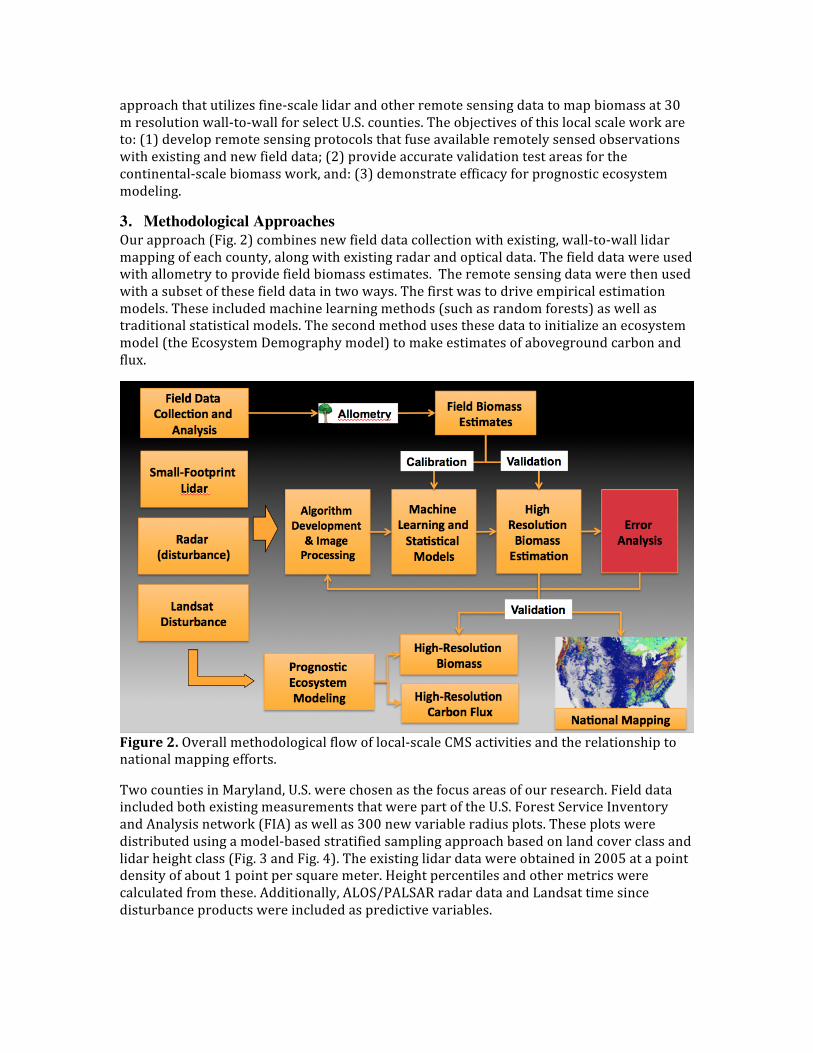
approach  that  utilizes  fine-­‐scale  lidar  and  other  remote  sensing  data  to  map  biomass  at  30  m  resolution  wall-­‐to-­‐wall  for  select  U.S.  counties.  The  objectives  of  this  local  scale  work  are  to:  (1)  develop  remote  sensing  protocols  that  fuse  available  remotely  sensed  observations  with  existing  and  new  field  data;  (2)  provide  accurate  validation  test  areas  for  the  continental-­‐scale  biomass  work,  and:  (3)  demonstrate  efficacy  for  prognostic  ecosystem  modeling.    

3. Methodological Approaches Our  approach  (Fig.  2)  combines  new  field  data  collection  with  existing,  wall-­‐to-­‐wall  lidar  mapping  of  each  county,  along  with  existing  radar  and  optical  data.  The  field  data  were  used  with  allometry  to  provide  field  biomass  estimates.    The  remote  sensing  data  were  then  used  with  a  subset  of  these  field  data  in  two  ways.  The  first  was  to  drive  empirical  estimation  models.  These  included  machine  learning  methods  (such  as  random  forests)  as  well  as  traditional  statistical  models.  The  second  method  uses  these  data  to  initialize  an  ecosystem  model  (the  Ecosystem  Demography  model)  to  make  estimates  of  aboveground  carbon  and  flux.      

Figure  2.  Overall  methodological  flow  of  local-­‐scale  CMS  activities  and  the  relationship  to  national  mapping  efforts.  

Two  counties  in  Maryland,  U.S.  were  chosen  as  the  focus  areas  of  our  research.  Field  data  included  both  existing  measurements  that  were  part  of  the  U.S.  Forest  Service  Inventory  and  Analysis  network  (FIA)  as  well  as  300  new  variable  radius  plots.  These  plots  were  distributed  using  a  model-­‐based  stratified  sampling  approach  based  on  land  cover  class  and  lidar  height  class  (Fig.  3  and  Fig.  4).  The  existing  lidar  data  were  obtained  in  2005  at  a  point  density  of  about  1  point  per  square  meter.  Height  percentiles  and  other  metrics  were  calculated  from  these.  Additionally,  ALOS/PALSAR  radar  data  and  Landsat  time  since  disturbance  products  were  included  as  predictive  variables.  

 

Figure  3.  Field  plots  were  placed  into  each  county  according  to  model-­‐based  stratification  based  on  NLCD  landcover  classes  (left)  and  height  classes  (right).  About  60  new  plots  were  placed  in  each  landcover  stratum,  and  distributed  equally  between  height  classes  in  that  stratum  (see  Fig  4.).  

 Figure  4.  Each  30  m  grid  cell  over  each  county  was  classified  into  one  of  the  strata  described  in  Fig.  3.  A  set  of  300  points  was  randomly  selected  (60  in  each  landcover  class)  and  sampled  for  biomass.  Because  of  the  suburban  nature  of  the  counties  points  could  fall  outside  of  forest  areas,  such  as  backyards,  road  medians,  and  agricultural  lands.    

At  each  plot,  prisms  were  used  to  identify  trees  within  and  outside  of  the  plot  (hence  the  plots  had  variable  radius).  This  resulted  in  about  7-­‐10  trees  for  inclusion  and  for  which  species  and  dbh  were  noted.  Jenkins  equations  were  then  used  to  obtain  allometric  aboveground  biomass  and  carbon.  The  USFS  additionally  created  20  new  FIA-­‐style  plots  and  another  20  variable  radius  plots  for  comparison.  These  were  in  addition  to  the  existing  FIA  plot  network  in  the  county  (which  is  quite  limited).  

3.1. Remote sensing data sets Small-­‐footprint  lidar  The  primary  remote  sensing  data  set  was  the  small  footprint  lidar  acquired  by  each  county.  These  data  were  flown  about  5  years  earlier  and  are  part  of  continuing  efforts  by  the  state  for  providing  up-­‐to  date  floodplain  mapping.  These  data  were  obtained  wall-­‐to-­‐wall  at  a  point  density  of  about  1  point/m^2.  The  first  and  last  return  data  were  then  used  to  derive  various  lidar  percentile  height  metrics.  These  percentiles  were  aggregated  using  a  2m  x  2  m  forest/non-­‐forest  cover  map  for  each  30  m  pixel  in  the  counties  (Fig.  5).  

 

Figure  5.  Lidar  height  metrics  were  derived  using  the  first  and  last  return  data  and  a  2m  x  2m  forest/non-­‐forest  map.  Heights  for  forested  areas  within  each  2m  pixel  were  then  aggregated  to  create  a  percentile  height  distribution  within  each  30  m  pixel,  from  which  height  metrics  were  derived.  

Landsat  time  since  disturbance  Disturbance  is  one  of  the  one  most  important  factors  affecting  biomass  dynamics.  Knowing  the  time  since  disturbance  provides  important  information  on  successional  state  (and  therefore  sequestration  potential,  especially  in  carbon  models)  and  also  for  biomass  loss  from  forest  patches  disturbed  after  lidar  data  collection.    A  30-­‐year  time  series  of  Landsat  data  were  used  to  create  the  disturbance  mosaic  shown  in  Fig.  6.  

 

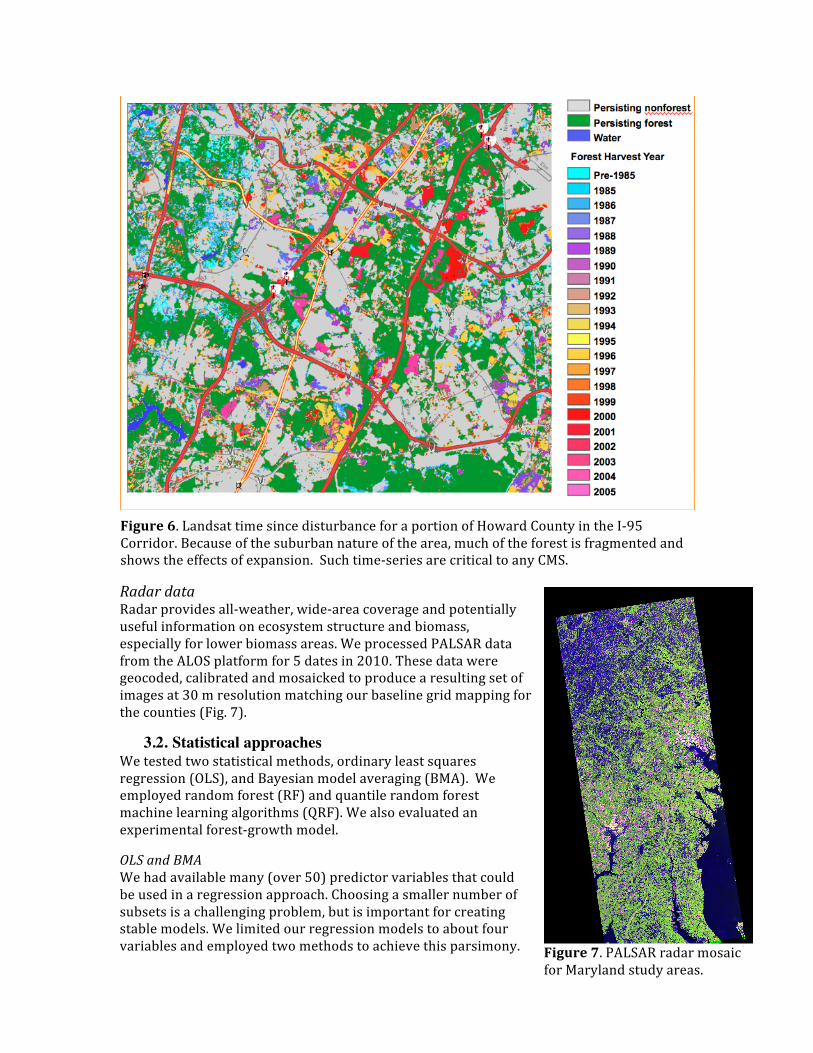
Radar  data  Radar  provides  all-­‐weather,  wide-­‐area  coverage  and  potentially  useful  information  on  ecosystem  structure  and  biomass,  especially  for  lower  biomass  areas.  We  processed  PALSAR  data  from  the  ALOS  platform  for  5  dates  in  2010.  These  data  were  geocoded,  calibrated  and  mosaicked  to  produce  a  resulting  set  of  images  at  30  m  resolution  matching  our  baseline  grid  mapping  for  the  counties  (Fig.  7).    

3.2. Statistical approaches We  tested  two  statistical  methods,  ordinary  least  squares  regression  (OLS),  and  Bayesian  model  averaging  (BMA).    We  employed  random  forest  (RF)  and  quantile  random  forest  machine  learning  algorithms  (QRF).  We  also  evaluated  an  experimental  forest-­‐growth  model.  

OLS  and  BMA  We  had  available  many  (over  50)  predictor  variables  that  could  be  used  in  a  regression  approach.  Choosing  a  smaller  number  of  subsets  is  a  challenging  problem,  but  is  important  for  creating  stable  models.  We  limited  our  regression  models  to  about  four  variables  and  employed  two  methods  to  achieve  this  parsimony.  

Figure  6.  Landsat  time  since  disturbance  for  a  portion  of  Howard  County  in  the  I-­‐95  Corridor.  Because  of  the  suburban  nature  of  the  area,  much  of  the  forest  is  fragmented  and  shows  the  effects  of  expansion.    Such  time-­‐series  are  critical  to  any  CMS.  

Figure  7.  PALSAR  radar  mosaic  for  Maryland  study  areas.  

The  first  is  a  method  called  “all-­‐possible  subsets”  that  iteratively  tries  all  combination  of  variables  and  chooses  the  ones  that  provide  the  most  explanatory  power  and  stability.  A  second  method,  called  Bayesian  Model  Averaging,  uses  a  Bayesian  approach  to  pick  variables.  

Random  forest  and  Quantile  Random  forest  Random  forest  is  a  now  well-­‐known  machine  learning  procedure  widely  employed  in  biomass  estimation.  It  suffers  from  a  common  problem  of  underestimation  of  high  biomass  values.  To  overcome  this  limitation  and  to  provide  robust  error  bounds,  we  employed  a  quantile  random  forest  approach.  Such  an  approach  predicts  not  the  median  value  (as  in  normal  random  forests)  but  a  particular  quantile.  This  allows  for  error  bounds  (say  5%  and  95%  quantiles)  to  be  predicted,  as  well  as  high  biomass  values  (large  quantiles).  As  far  as  we  know  this  is  the  first  time  such  an  approach  has  been  used  for  biomass  estimation.  

4. Carbon Modeling Efforts The  ability  to  evaluate  future  carbon  states  rests  firmly  in  the  domain  of  physically-­‐based  ecosystem  models.  Such  models  predict  not  only  biomass,  but  carbon  flux  now  and  in  the  future.  To  be  effective  these  models  require  accurate  initialization  data,  most  importantly,  current  forest  status  (age  and  structure).  In  addition,  information  on  climate  and  soils  is  also  required.  We  used  the  Ecosystem  Demography  model  (ED)  for  our  efforts  here.  No  ecosystem  model  has  been  run  at  the  resolution  of  our  county  data  (1  ha)  over  such  a  large  area  (and  indeed  the  computation  effort  was  equivalent  to  running  ED  globally  at  coarse  resolution).  

Climatological  and  soil  data  were  obtained  and  processed  for  the  counties.  Then  a  series  of  experiments  was  performed  to  evaluate  the  effect  of  increasing  resolution  and  adding  successional  state  and  structure  to  the  models,  that  is  going  from  what  is  basically  a  potential  vegetation  model  to  one  that  is  predicting  actual  carbon  status  at  the  resolution  required.    A  summary  of  these  experiments  is  given  in  Fig.  8.  

 

 

 

Figure  8.  ED  was  run  using  a  variety  of  input  layers  at  varying  resolutions,  with  V1.6  the  most  sophisticated.  

Use  of  the  ED  model  also  required  detailed  model  species  allometry  refinements  to  run  at  such  high  resolutions  for  the  mid-­‐atlantic  region.  This  required  a  considerable  validation  effort  (Fig.  9).  

5. Results 5.1. Empirical modeling

We  compared  our  four  models  (OLS,  BMA,  RF  &  QRF).  Results  were  similar,  with  RMSE  values  of  79,  75,  66.5  and  63  Mg/ha  for  OLS,  BMA,  RF  and  QRF,  respectively  (Fig.  10).  Total  county  biomass  (Fig.  11)  compared  well  in  all  methods.  Results  also  compared  well  with  estimates  from  FIA  for  forested  lands  (e.g  13.6  Tg  for  CMS  vs  13.5  Tg).  However,  FIA  estimates  for  non-­‐forest  (e.g.  urban  and  suburban  areas)  were  much  lower  than  CMS  estimates  (2.1  Tg  vs.  5.6  Tg)  (Fig.  12).  Maps  of  biomass  from  each  method  were  generally  quite  similar,  but  showed  some  variation  at  local  scales  (Fig.  13).  

 

 

 

Figure  9.  ED  species  curve  validations.  DBH/biomass  for  individual  species  curves  are  shown.  ED  uses  a  generalized  allometric  equations  to  represent  different  functional  types.  The  ED  model  correctly  captured  the  correct  relationships  after  adjustment  for  use  in  CMS.  

 

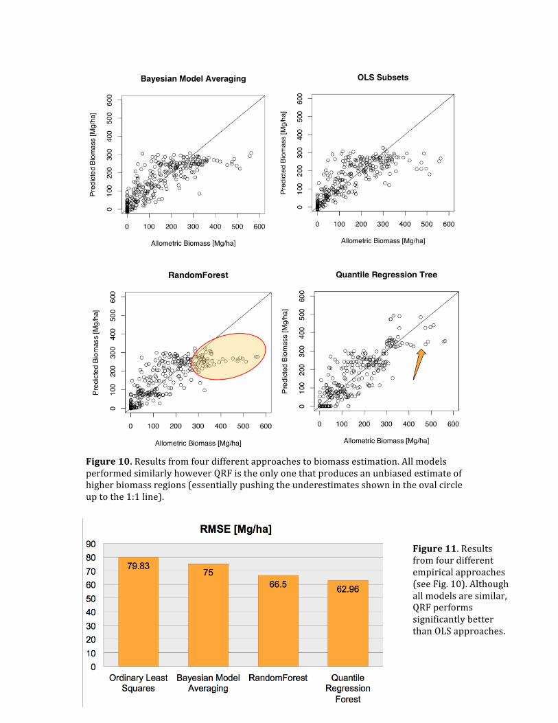
Figure  10.  Results  from  four  different  approaches  to  biomass  estimation.  All  models  performed  similarly  however  QRF  is  the  only  one  that  produces  an  unbiased  estimate  of  higher  biomass  regions  (essentially  pushing  the  underestimates  shown  in  the  oval  circle  up  to  the  1:1  line).  

 

Figure  11.  Results  from  four  different  empirical  approaches  (see  Fig.  10).  Although  all  models  are  similar,  QRF  performs  significantly  better  than  OLS  approaches.  

 

Figure  12.  Comparison  of  one  CMS  estimate  (BMA)  of  biomass  with  USFS-­‐FIA  plot  estimates.  Model  and  USFS  results  are  essentially  identical  of  forested  areas  (that  is  areas  classified  as  forest  by  NLCD),  but  diverge  strongly  for  non-­‐forest  areas.  This  is  a  reflection  of  the  fragmented  and  suburban  nature  of  the  counties  and  shows  that  non-­‐forest  areas  are  a  significant  pool  of  carbon  that  must  be  accounted  for  properly.  

 

Figure  13.  Above  ground  biomass  for  two  Maryland  counties.  Map  shown  on  left  was  generated  using  the  BMA  approach.  Insets  show  detail  of  maps  generated  using  different  methods  and  visible  imagery  of  the  inset  (bottom  right).  

Error  maps  Providing  estimates  of  uncertainty  is  critical  for  CMS.  Both  OLS  and  QRF  provide  clear  and  theoretically  sound  bases  for  providing  such  maps.  Shown  below  (Fig.  14)  is  one  such  example  (generated  for  BMA).  For  any  30  m  pixel  in  the  counties,  the  5%  and  95%  confidence  interval  is  known.    

 

Figure  14.  Error  maps  from  BMA  biomass  predictions.  Note  that  the  lower  and  upper  bound  maps  give  the  95%  confidence  interval  for  any  particular  30  m  pixel.    

5.2. Radar modeling Biomass  was  also  estimated  using  radar  data  alone.  These  results  are  similar  to  other  radar  modeling  efforts,  with  saturation  at  high  biomass  (Fig.  15)  

!"#"$%$$&'()*+","$%$$-."/0"#"$%&$1.1"

!"#"$%$$23'()*+","$%$$&&"/0"#"$%445-3"

!"#"$%$$2'()*+","$%$$&5"/0"#"$%41212"

!"#"$%$$6'()*+"7"$%$$$."/0"#"$%4$261"

!"#"$%$$6-'()*+","$%$$1."/0"#"$%-62-5"

$"

$%$3"

$%$1"

$%$5"

$%$-"

$%$4"

$%$&"

$%$."

$" 4$" 3$$" 34$" 1$$" 14$" 5$$"

!"#$%#"&

'()*+

,-'(.)

/0,1'2(,345)!6,7"%%)*829:".)

;'<"=,4%:6>)0'?-''4)86@'5)A,('%?)/B!)"45)CD0"45)0"#$%#"&'()5'>'45642),4)"E36%6=,4)5"?')64)8"(F<"45)

89:;9<=9>"

?@!"

AB'!"

CBDBE;"

FG;H=9>"

!"#"$%$$&'()*+,"-"$%$$.&"/0"#"$%121$."

$"

$%$$2"

$%$'"

$%$'2"

$%$3"

$%$32"

$%$."

$%$.2"

$%$4"

$%$42"

$%$2"

$" 2$" '$$" '2$" 3$$" 32$" .$$" .2$"

!"#"

$%&"'()'"*+$%,-

./+$0%

12.3+4$.56#%&7.8"))%,94:;"0%

!+<"=.6);7>%2+?/++6%<73+%1@&%"6#%AB%2"'()'"*+$%76%97C+#%D.$+)?)%E$.8%?+8>.$"<%"3+$"4764%.E%78"4+)%76%9"$F<"6#%

Figure  15.  Relationship  between  PALSAR  backscatter  and  biomass.  Temporal  averaging  strengthens  the  relationship  but  still  saturates  at  higher  levels  of  biomass.  Radar  metrics  were  not  picked  by  regression  and  machine  learning  models  (mainly  because  of  domination  by  lidar  metrics).  

5.3. ED carbon modeling The  ED  model  was  run  for  the  cases  outlined  earlier,  from  the  simplest  (and  in  theory  least  accurate)  realization  using  no  canopy  structure  and  1  degree  climate  and  soil  inputs,  up  to  the  most  refined  realization,  using  actual  canopy  heights  from  lidar,  Landsat  disturbance,  1  ha  soils,  and  0.25  degree  climate.  The  results  are  summarized  in  Fig.  14  and  maps  of  biomass  are  shown  in  Fig.  15.  

 

Figure  14.  Results  from  ED  experiments.  Using  no  height  initialization  and  coarse  soils  and  climate  (V1.0  and  left  Fig.  15)  results  in  far  different  biomass  estimates  relative  to  using  lidar  height  initializationand  fine-­‐scale  soils  and  climate  (V1.6  and  right  Fig.  15).  

 

Figure  15.  ED  biomass  results  for  V1.0  (left)  and  V1.6  (right).  Clearly,  carbon  models  must  use  high-­‐resolution  inputs  to  be  effective  for  most  CMS  activities.  

 

 

6. Considerations and Conclusions

Given  the  staleness  of  our  lidar  data  and  our  limited  field  sampling,  our  results  were  quite  encouraging.  We  conclude  the  following:  (1)  Existing  lidar  data  sets  are  useful  for  biomass  mapping  in  the  U.S.  at  local  scales,  even  if  they  are  several  years  old  and  of  low  point  density;  (2)  Rapid  field-­‐survey  methods  are  accurate  and  appropriate;  (3)  Choice  of  statistical  estimation  method  is  not  critical,  though  some  methods  appear  more  accurate;  (4)  High-­‐resolution  mapping  is  required  to  accurately  estimate  non-­‐forest  biomass;  (5)  County-­‐based  lidar  data  sets  should  form  the  basis  of  local  CMS  efforts,  both  in  the  U.S.  and  abroad;  (6)  Carbon  modeling  is  critical  but  must  have  appropriate  input  data;  in  particular  high-­‐resolution  canopy  structure  data  and  soils.