Convex Optimization — Boyd & Vandenberghe

10. Unconstrained minimization

• terminology and assumptions

• gradient descent method

• steepest descent method

• Newton’s method

• self-concordant functions

• implementation

10–1

Unconstrained minimization

minimize f(x)

• f convex, twice continuously differentiable (hence dom f open)

⋆ • we assume optimal value p = infx f(x) is attained (and finite)

unconstrained minimization methods

• produce sequence of points x(k) ∈ dom f , k = 0, 1, . . . with

f(x(k)) → p ⋆

• can be interpreted as iterative methods for solving optimality condition

∇f(x ⋆ ) = 0

Unconstrained minimization 10–2

�

Initial point and sublevel set

algorithms in this chapter require a starting point x(0) such that

• x(0) ∈ dom f

• sublevel set S = {x | f(x) ≤ f(x(0))} is closed

2nd condition is hard to verify, except when all sublevel sets are closed:

• equivalent to condition that epi f is closed

• true if dom f = Rn

• true if f(x) → ∞ as x → bddom f

examples of differentiable functions with closed sublevel sets:

f(x) = log( exp(aT i x + bi)), f(x) = − log(bi − aT

i x)

m m�

Unconstrained minimization 10–3

i=1 i=1

Strong convexity and implications

f is strongly convex on S if there exists an m > 0 such that

∇2f(x) � mI for all x ∈ S

implications

• for x, y ∈ S,

f(y) ≥ f(x) + ∇f(x)T (y − x) + m �x − y�2

22

hence, S is bounded

• p ⋆ > −∞, and for x ∈ S,

f(x) − p ⋆ ≤ 1 �∇f(x)�2

22m

useful as stopping criterion (if you know m)

Unconstrained minimization 10–4

Descent methods

x(k+1) = x(k) + t(k)Δx(k) with f(x(k+1)) < f(x(k))

• other notations: x+ = x + tΔx, x := x + tΔx

• Δx is the step, or search direction; t is the step size, or step length

• from convexity, f(x+) < f(x) implies ∇f(x)TΔx < 0 (i.e., Δx is a descent direction)

General descent method.

given a starting point x ∈ dom f .

repeat

1. Determine a descent direction Δx.

2. Line search. Choose a step size t > 0.

3. Update. x := x + tΔx.

until stopping criterion is satisfied.

Unconstrained minimization 10–5

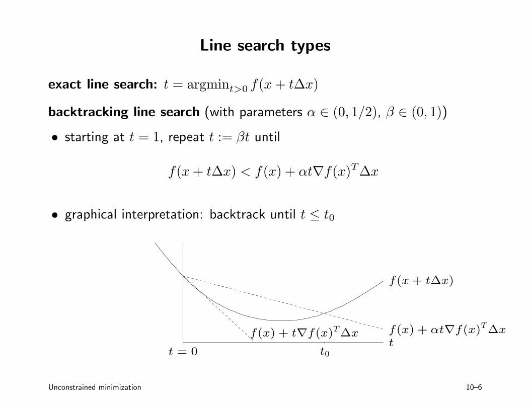
Line search types

exact line search: t = argmint>0 f(x + tΔx)

backtracking line search (with parameters α ∈ (0, 1/2), β ∈ (0, 1))

• starting at t = 1, repeat t := βt until

f(x + tΔx) < f(x) + αt∇f(x)TΔx

• graphical interpretation: backtrack until t ≤ t0

t = 0 t0

f(x + tΔx)

f(x) + t∇f(x)TΔx f(x) + αt∇f(x)TΔx t

Unconstrained minimization 10–6

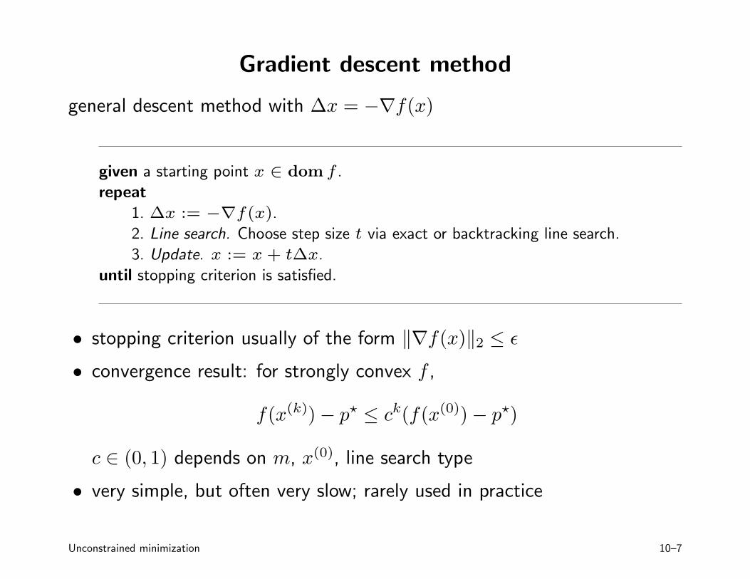
Gradient descent method

general descent method with Δx = −∇f(x)

given a starting point x ∈ dom f .

repeat

1. Δx := −∇f(x).

2. Line search. Choose step size t via exact or backtracking line search.

3. Update. x := x + tΔx.

until stopping criterion is satisfied.

• stopping criterion usually of the form �∇f(x)�2 ≤ ǫ

• convergence result: for strongly convex f ,

f(x(k)) − p ⋆ ≤ c k(f(x(0)) − p ⋆ )

c ∈ (0, 1) depends on m, x(0), line search type

• very simple, but often very slow; rarely used in practice

Unconstrained minimization 10–7

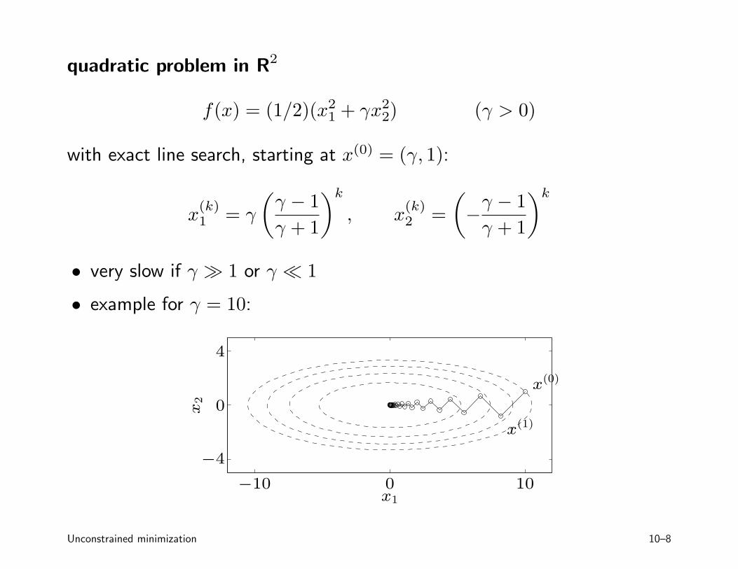
quadratic problem in R2

f(x) = (1/2)(x 21 + γx22) (γ > 0)

with exact line search, starting at x(0) = (γ, 1):

�γ − 1

�k � γ − 1

�k

x(1 k)

= γ , x(2 k)

= − γ + 1 γ + 1

• very slow if γ ≫ 1 or γ ≪ 1

• example for γ = 10:

x2

x(0)

x(1)

0

4

−4

−10 0 10 x1

Unconstrained minimization 10–8

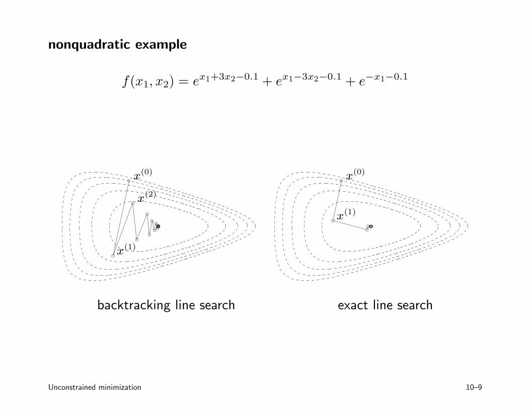
nonquadratic example

f(x1, x2) = e x1+3x2−0.1 + e x1−3x2−0.1 + e −x1−0.1

x(0)

x(1)

x(2)

x(0)

x(1)

backtracking line search exact line search

Unconstrained minimization 10–9

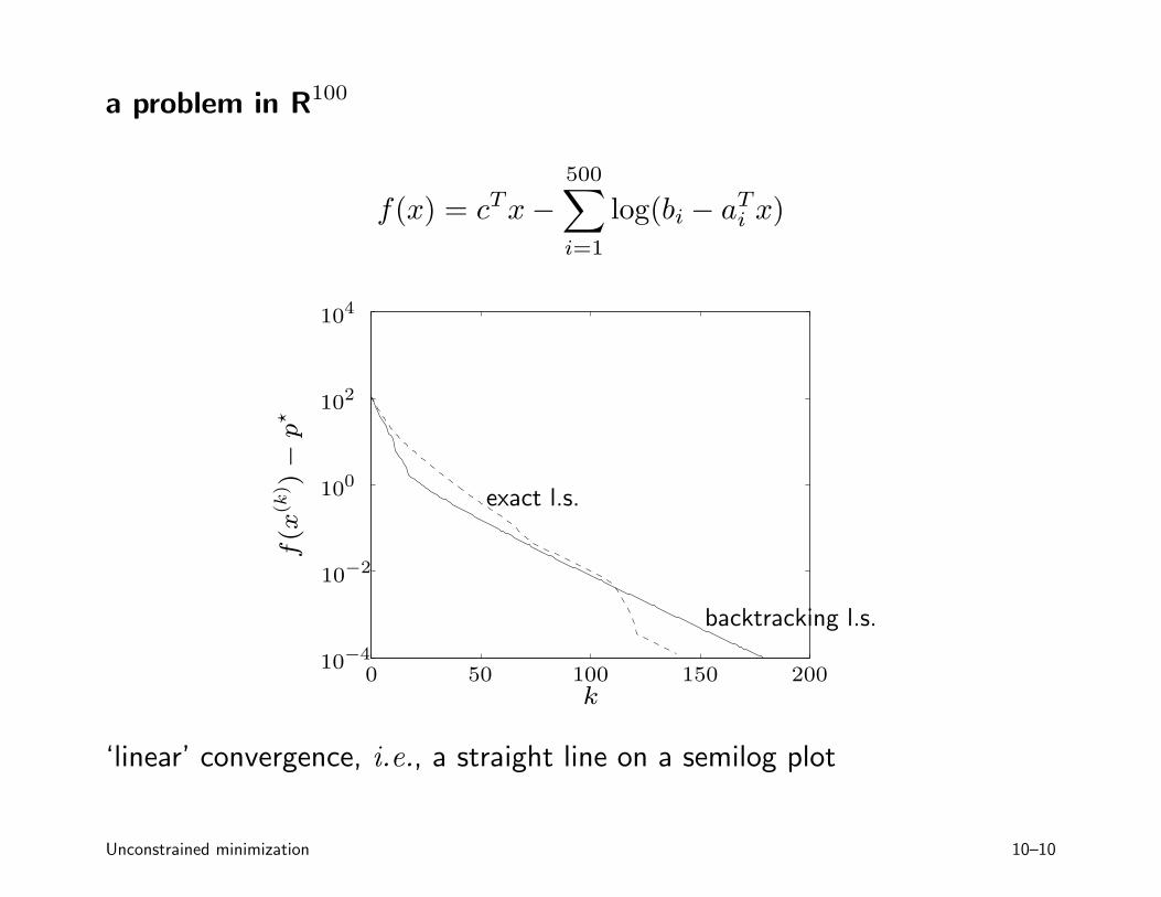
a problem in R100

500

f(x) = c T x −�

log(bi − a Ti x) i=1

104

0 50 100 150 200k

f(x

(k) )

−p ⋆

exact l.s.

backtracking l.s.

10−4

10−2

100

102

‘linear’ convergence, i.e., a straight line on a semilog plot

Unconstrained minimization 10–10

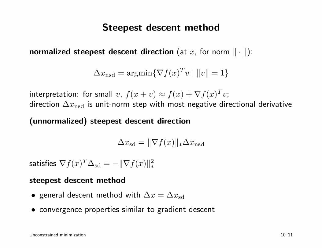
Steepest descent method

normalized steepest descent direction (at x, for norm � · �):

Δxnsd = argmin{∇f(x)T v | �v� = 1}

interpretation: for small v, f(x + v) ≈ f(x) + ∇f(x)Tv; direction Δxnsd is unit-norm step with most negative directional derivative

(unnormalized) steepest descent direction

Δxsd = �∇f(x)�∗Δxnsd

satisfies ∇f(x)TΔsd = −�∇f(x)�2 ∗

steepest descent method

• general descent method with Δx = Δxsd

• convergence properties similar to gradient descent

Unconstrained minimization 10–11

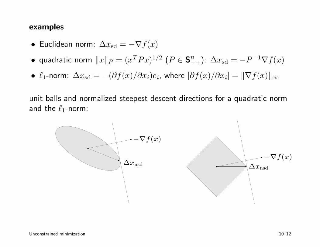
examples

• Euclidean norm: Δxsd = −∇f(x)

• quadratic norm �x�P = (xTPx)1/2 (P ∈ Sn ): −P −1∇f(x)++ Δxsd =

• ℓ1-norm: Δxsd = −(∂f(x)/∂xi)ei, where |∂f(x)/∂xi| = �∇f(x)�∞

unit balls and normalized steepest descent directions for a quadratic norm and the ℓ1-norm:

Δxnsd

−∇f(x)

−∇f(x)

Δxnsd

Unconstrained minimization 10–12

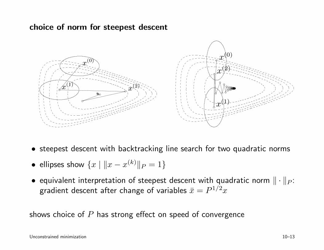
choice of norm for steepest descent

x(0)

x(1) x(2)

x(0)

x(1)

x(2)

• steepest descent with backtracking line search for two quadratic norms

• ellipses show {x | �x − x(k)�P = 1}

• equivalent interpretation of steepest descent with quadratic norm � · �P : gradient descent after change of variables x̄ = P 1/2x

shows choice of P has strong effect on speed of convergence

Unconstrained minimization 10–13

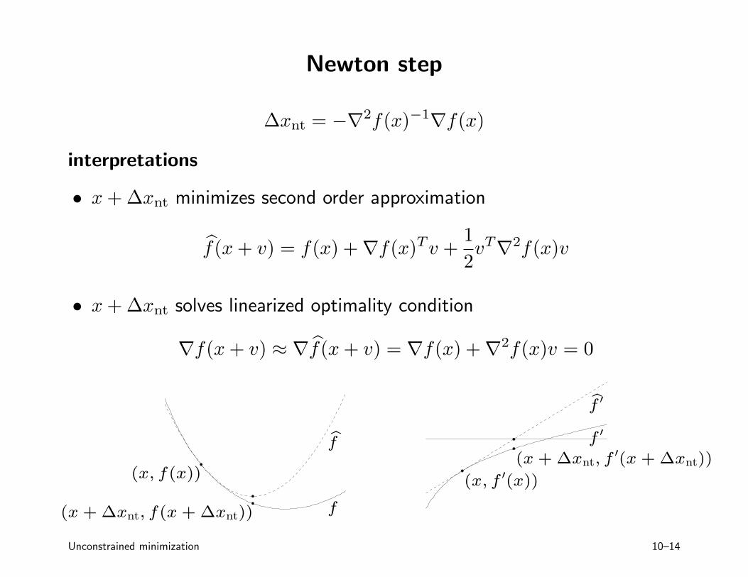
Newton step

Δxnt = −∇2f(x)−1∇f(x)

interpretations

• x + Δxnt minimizes second order approximation

f�(x + v) = f(x) + ∇f(x)T v +2

1 v T∇2f(x)v

• x + Δxnt solves linearized optimality condition

∇f(x + v) ≈ ∇f�(x + v) = ∇f(x) + ∇2f(x)v = 0

f

bf

(x, f(x))

(x + Δxnt, f(x + Δxnt))

f ′

bf ′

(x, f ′ (x))

(x + Δxnt, f ′ (x + Δxnt))

Unconstrained minimization 10–14

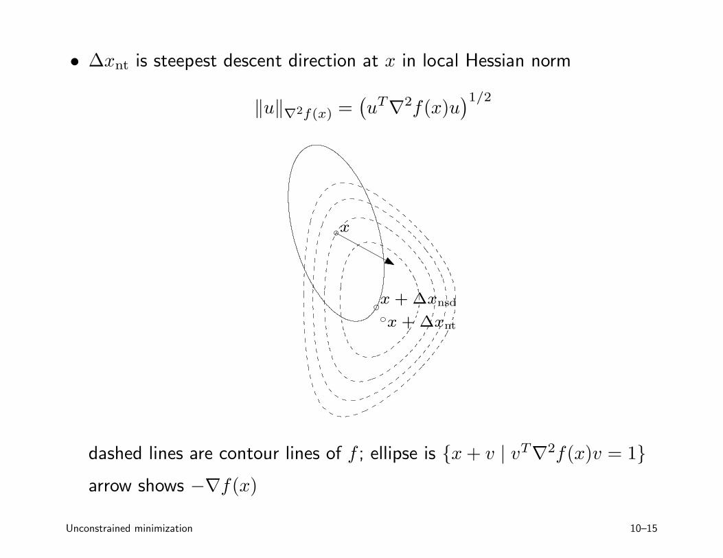
• Δxnt is steepest descent direction at x in local Hessian norm

�u�∇2f(x) = �u T∇2f(x)u

�1/2

x

x + Δxnt

x + Δxnsd

dashed lines are contour lines of f ; ellipse is {x + v | vT∇2f(x)v = 1}

arrow shows −∇f(x)

Unconstrained minimization 10–15

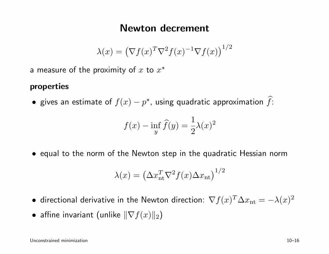
Newton decrement

λ(x) = �∇f(x)T∇2f(x)−1∇f(x)

�1/2

⋆a measure of the proximity of x to x

properties

• gives an estimate of f(x) − p ⋆, using quadratic approximation f�:

1 λ(x)2f(x) − inf f(y) =

y �

2

• equal to the norm of the Newton step in the quadratic Hessian norm

λ(x) = �Δxnt

T ∇2f(x)Δxnt

�1/2

• directional derivative in the Newton direction: ∇f(x)TΔxnt = −λ(x)2

• affine invariant (unlike �∇f(x)�2)

Unconstrained minimization 10–16

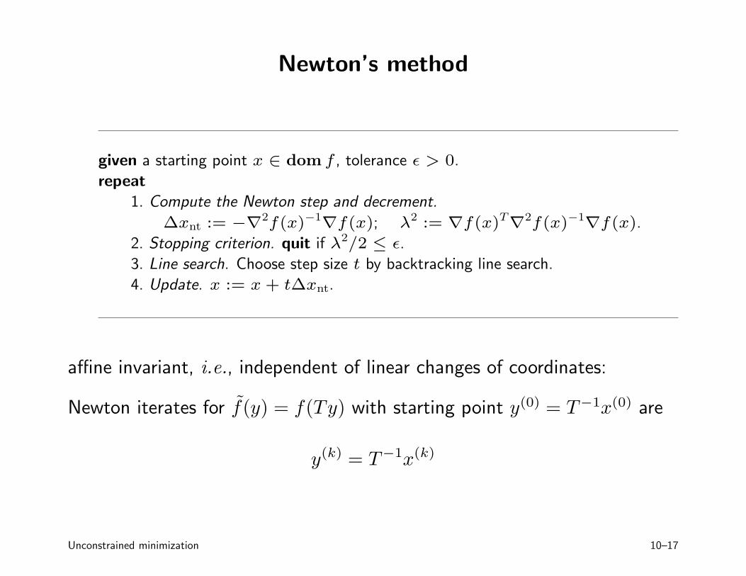
Newton’s method

given a starting point x ∈ dom f , tolerance ǫ > 0.

repeat

1. Compute the Newton step and decrement. Δxnt := −∇2f(x)−1∇f(x); λ2 := ∇f(x)T∇2f(x)−1∇f(x).

2. Stopping criterion. quit if λ2/2 ≤ ǫ.

3. Line search. Choose step size t by backtracking line search.

4. Update. x := x + tΔxnt.

affine invariant, i.e., independent of linear changes of coordinates:

Newton iterates for f̃(y) = f(Ty) with starting point y(0) = T −1x(0) are

y(k) = T −1 x(k)

Unconstrained minimization 10–17

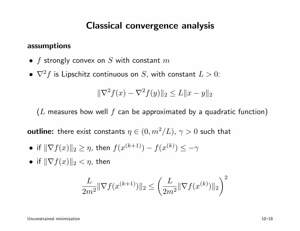
Classical convergence analysis

assumptions

• f strongly convex on S with constant m

• ∇2f is Lipschitz continuous on S, with constant L > 0:

�∇2f(x) −∇2f(y)�2 ≤ L�x − y�2

(L measures how well f can be approximated by a quadratic function)

outline: there exist constants η ∈ (0,m2/L), γ > 0 such that

• if �∇f(x)�2 ≥ η, then f(x(k+1)) − f(x(k)) ≤ −γ

• if �∇f(x)�2 < η, then

L �∇f(x(k+1))�2 ≤

� L

�∇f(x(k))�2

�2

2m2 2m2

Unconstrained minimization 10–18

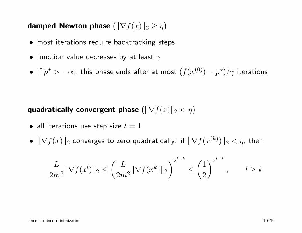
damped Newton phase (�∇f(x)�2 ≥ η)

• most iterations require backtracking steps

• function value decreases by at least γ

• if p ⋆ > −∞, this phase ends after at most (f(x(0)) − p ⋆)/γ iterations

quadratically convergent phase (�∇f(x)�2 < η)

• all iterations use step size t = 1

• �∇f(x)�2 converges to zero quadratically: if �∇f(x(k))�2 < η, then

L �

L �2l−k �

1�2l−k

�∇f(x l)�2 ≤ �∇f(x k)�2 ≤ , l ≥ k 2m2 2m2 2

Unconstrained minimization 10–19

conclusion: number of iterations until f(x) − p ⋆ ≤ ǫ is bounded above by

f(x(0)) − p ⋆

+ log2 log2(ǫ0/ǫ)γ

• γ, ǫ0 are constants that depend on m, L, x(0)

• second term is small (of the order of 6) and almost constant for practical purposes

• in practice, constants m, L (hence γ, ǫ0) are usually unknown

• provides qualitative insight in convergence properties (i.e., explains two algorithm phases)

Unconstrained minimization 10–20

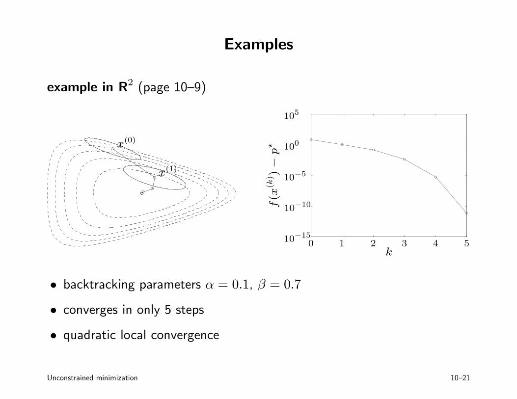
Examples

example in R2 (page 10–9)

105

x(0)

x(1)

f(x

(k) )

−p

⋆

100

10−5

10−10

10−15 0 1 2 3 4 5

k

• backtracking parameters α = 0.1, β = 0.7

• converges in only 5 steps

• quadratic local convergence

Unconstrained minimization 10–21

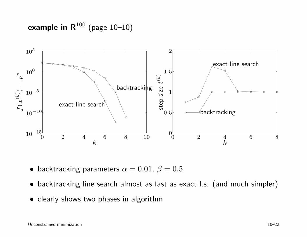
example in R100 (page 10–10)

2105

exact line search 1.5100

backtracking

backtracking

10−10

exact line search 0.5

step

siz

e t (k

)

10−5 1

10−15 0 0 2 4 6 8 10 0 2 4 6

k k

• backtracking parameters α = 0.01, β = 0.5

• backtracking line search almost as fast as exact l.s. (and much simpler)

• clearly shows two phases in algorithm

Unconstrained minimization 10–22

f(x

(k) )

−p

⋆

8

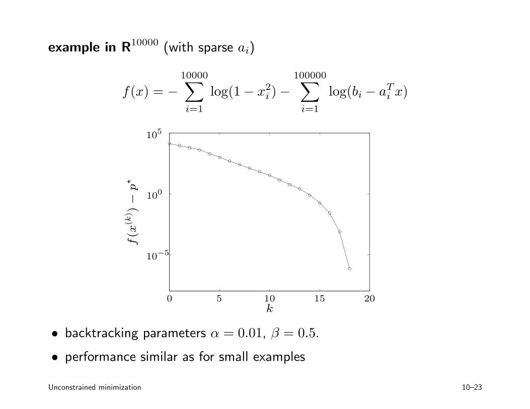
example in R10000 (with sparse ai)

10000 100000

f(x) = − �

log(1 − xi2) −

� log(bi − ai

T x) i=1 i=1

105 f(x

(k) )

−p ⋆

10−5

100

0 5 10 15 20 k

• backtracking parameters α = 0.01, β = 0.5.

• performance similar as for small examples

Unconstrained minimization 10–23

Self-concordance

shortcomings of classical convergence analysis

• depends on unknown constants (m, L, . . . )

• bound is not affinely invariant, although Newton’s method is

convergence analysis via self-concordance (Nesterov and Nemirovski)

• does not depend on any unknown constants

• gives affine-invariant bound

• applies to special class of convex functions (‘self-concordant’ functions)

• developed to analyze polynomial-time interior-point methods for convex optimization

Unconstrained minimization 10–24

Self-concordant functions

definition

• convex f : R → R is self-concordant if |f ′′′ (x)| ≤ 2f ′′ (x)3/2 for all x ∈ dom f

• f : Rn → R is self-concordant if g(t) = f(x + tv) is self-concordant for all x ∈ dom f , v ∈ Rn

examples on R

• linear and quadratic functions

• negative logarithm f(x) = − log x

• negative entropy plus negative logarithm: f(x) = x log x − log x

affine invariance: if f : R → R is s.c., then f̃(y) = f(ay + b) is s.c.:

f̃ ′′′ (y) 3f ′′′ (ay + b), f̃ ′′ (y) 2f ′′ (ay + b)= a = a

Unconstrained minimization 10–25

Self-concordant calculus

properties

• preserved under positive scaling α ≥ 1, and sum

• preserved under composition with affine function

• if g is convex with dom g = R++ and |g ′′′ (x)| ≤ 3g ′′ (x)/x then

f(x) = log(−g(x)) − log x

is self-concordant

examples: properties can be used to show that the following are s.c.

• f(x) = −�m

i=1 log(bi − aiTx) on {x | ai

Tx < bi, i = 1, . . . ,m}

• f(X) = − log detX on Sn ++

• f(x) = − log(y2 − xTx) on {(x, y) | �x�2 < y}

Unconstrained minimization 10–26

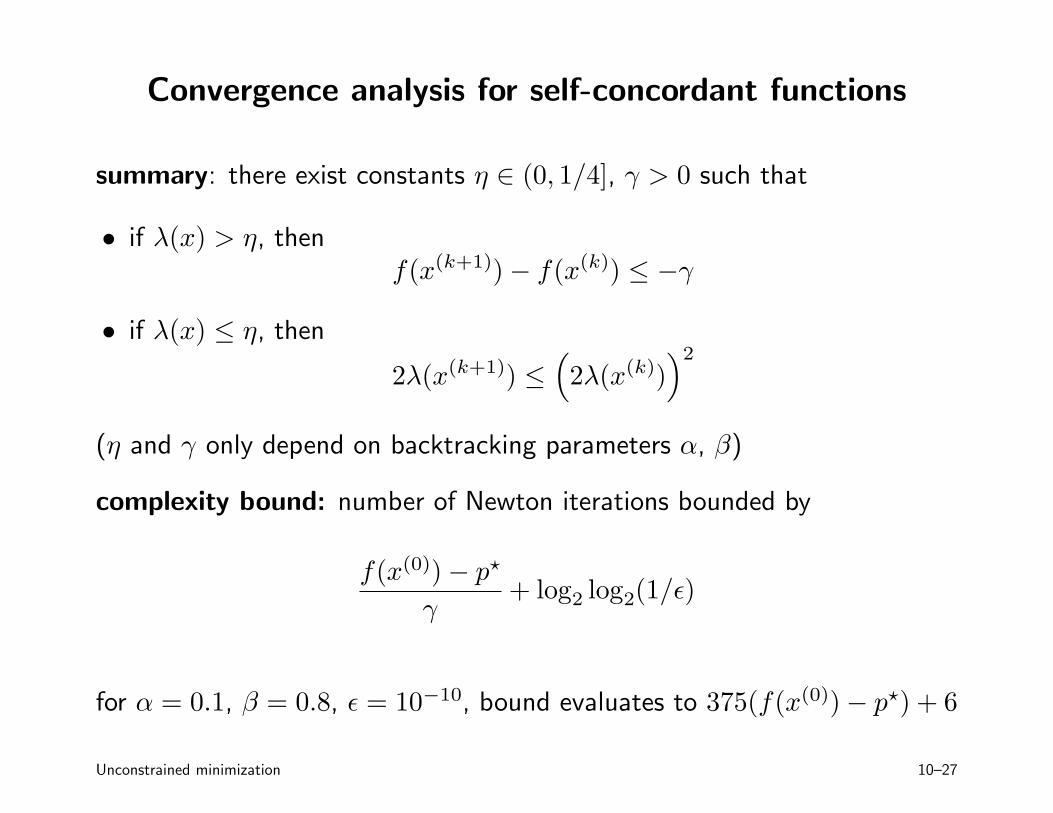
Convergence analysis for self-concordant functions

summary: there exist constants η ∈ (0, 1/4], γ > 0 such that

• if λ(x) > η, then f(x(k+1)) − f(x(k)) ≤ −γ

• if λ(x) ≤ η, then

2λ(x(k+1)) ≤ �2λ(x(k))

�2

(η and γ only depend on backtracking parameters α, β)

complexity bound: number of Newton iterations bounded by

f(x(0)) − p ⋆

+ log2 log2(1/ǫ)γ

for α = 0.1, β = 0.8, ǫ = 10−10, bound evaluates to 375(f(x(0)) − p ⋆) + 6

Unconstrained minimization 10–27

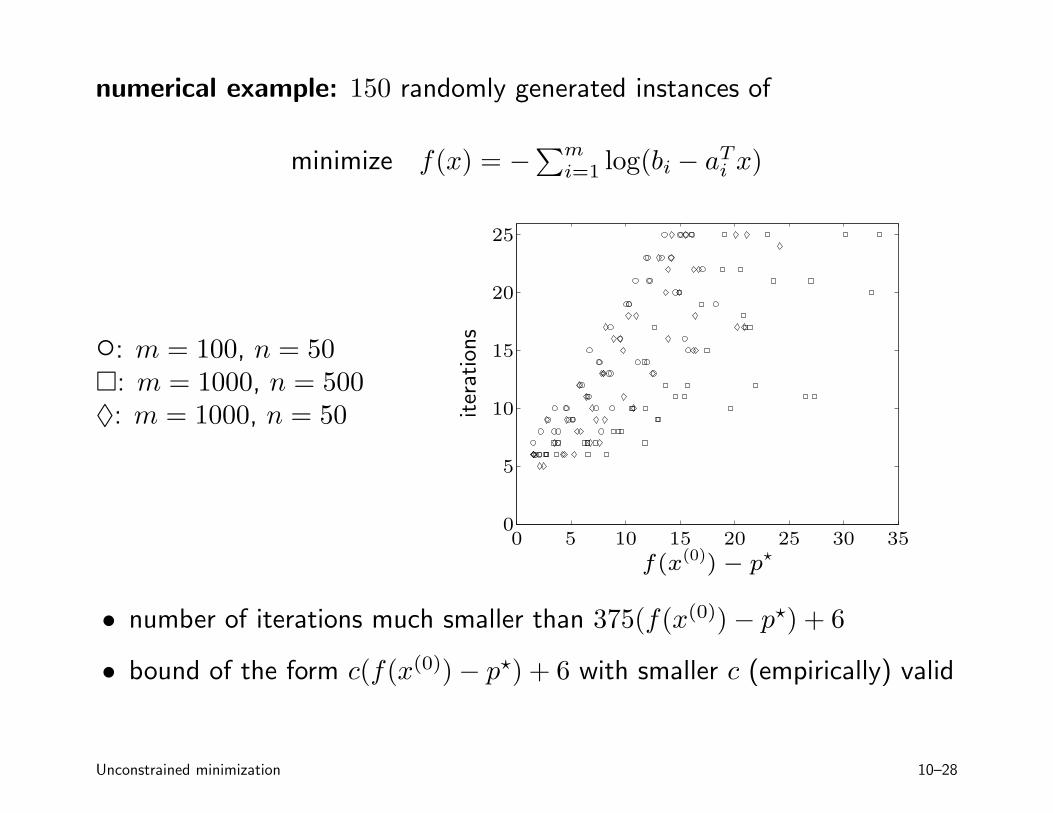
numerical example: 150 randomly generated instances of

Tminimize f(x) = −�m

i=1 log(bi − ai x)

25

20

◦: m = 100, n = 50�: m = 1000, n = 500♦: m = 1000, n = 50 it

erat

ions

15

10

5

0 0 5 10 15 20 25 30 35

f(x(0)) − p⋆

• number of iterations much smaller than 375(f(x(0)) − p ⋆) + 6

• bound of the form c(f(x(0)) − p ⋆) + 6 with smaller c (empirically) valid

Unconstrained minimization 10–28

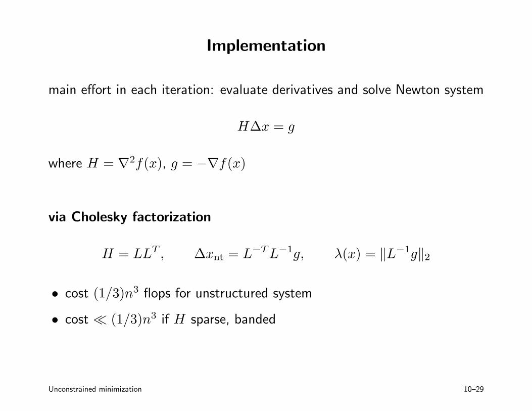
Implementation

main effort in each iteration: evaluate derivatives and solve Newton system

HΔx = g

where H = ∇2f(x), g = −∇f(x)

via Cholesky factorization

H = LLT , Δxnt = L−TL−1 g, λ(x) = �L−1 g�2

• cost (1/3)n3 flops for unstructured system

• cost ≪ (1/3)n3 if H sparse, banded

Unconstrained minimization 10–29

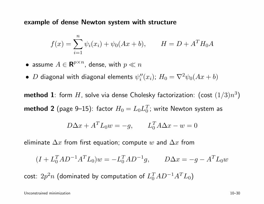
example of dense Newton system with structure

n

f(x) = �

ψi(xi) + ψ0(Ax + b), H = D + ATH0A i=1

• assume A ∈ Rp×n, dense, with p ≪ n

• D diagonal with diagonal elements ψi ′′ (xi); H0 = ∇2ψ0(Ax + b)

method 1: form H, solve via dense Cholesky factorization: (cost (1/3)n3)

method 2 (page 9–15): factor H0 = L0L0 T ; write Newton system as

DΔx + ATL0w = −g, LT 0 AΔx − w = 0

eliminate Δx from first equation; compute w and Δx from

(I + LT 0 AD

−1ATL0)w = −LT 0 AD

−1 g, DΔx = −g −ATL0w

cost: 2p2n (dominated by computation of LT 0 AD

−1ATL0)

Unconstrained minimization 10–30

MIT OpenCourseWare http://ocw.mit.edu

6.079 / 6.975 Introduction to Convex Optimization Fall 2009

For information about citing these materials or our Terms of Use, visit: http://ocw.mit.edu/terms.