NEW ECONOMIC SCHOOLMasters in Energy Economics - Masters in Finance

Data Analysis in PythonModule 2, 2016–2017

Professor: Stanislav KhrapovNew Economic School

skhrapov@nes.ru

Course information

Course Website: my.nes.ruInstructor’s Office Hours: Just knock on the doorClass Time: TBARoom Number: TBATA: Emil Lakkis (elakkis@nes.ru)

Course description

The course is an introduction to statistical data analysis based on open source software ecosystem ofPython. Modern industry is overwhelmed by the amount of data it can collect. At the same time thetools that are used to process, analyze, and visualize the data are expensive and outdated. These daysdata crunching becomes increasingly the domain of free open source programming languages such asPython. Hence, the goal of this course is to give the students tools to process large amount of dataefficiently, summarize it, visualize it, and make informative decisions based on that. Students shouldlearn how to clean imperfectly collected data, how to aggregate it, dissect it, and present the results forefficient communication using state-of-the-art graphing capabilities of Python.

Course requirements and grading

The grading of student’s performance is based on

• 5 weekly individual homework assignments that account for 20% of the final grade.

Homework assignments will contain practical computational exercises to be written in Python.They will be posted on my.nes.ru. Your individual work must be uploaded on my.nes.ru before thespecified deadline. Late submissions have zero weight. Sloppy formatting is heavily penalized.The homework should contain at most two separate files:

1

– Pdf report with text, graphics, and tables.

– Working bug-free code.

• Final exam accounts for 80% of the final grade.

The exam will be conducted in one of the computer classes with no Internet access. Pythonenvironment will be preinstalled. All necessary manuals and reference material will be provided.

• The format of the make-up exam is the same as the final.

Course materials

Required textbooks and materials

• My own lecture notes <dataanalysispython.readthedocs.org>

• Python Scientific Lecture Notes <scipy-lectures.github.io>

• Dive into Python 3 <diveintopython3.net>

Additional materials

• Pandas - Python data analysis library <pandas.pydata.org>

• Matplotlib - plotting library <matplotlib.org>

• Bokeh - Interactive plotting <bokeh.pydata.org>

• Plotly - Interactive plotting <plot.ly>

Academic integrity policy

Cheating, plagiarism, and any other violations of academic ethics at NES are not tolerated.

Course contents

1 Python basics

• Datatypes: lists, tuples, dictionaries, strings, numbers, booleans

• Comprehensions

2

• Control flow

• Functions, classes

• Reusing code

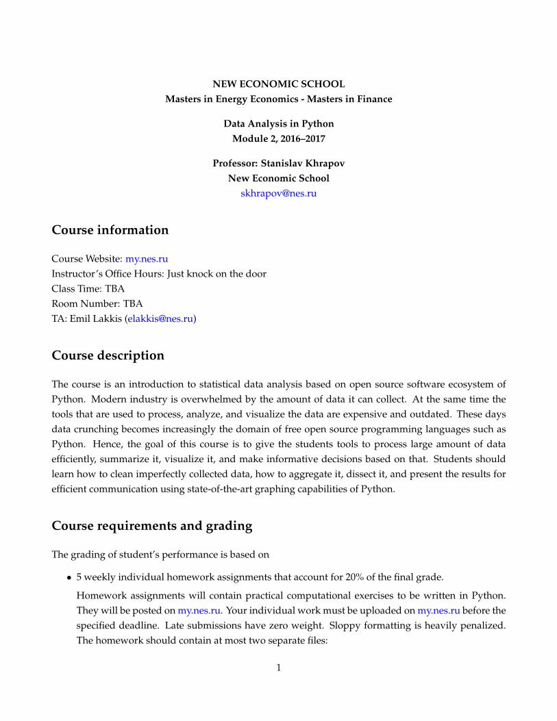
2 Data processing

• Loading data from the web, csv, Excel

• Data structures: Series, DataFrame, Panel

• Merging several data sets

• Indexing and selecting data

• Computational tools for data modification

• Grouping and aggregating data

• Reshaping data

• Time and date functionality

3 Data visualization

• Creating simple plots: line, scatter, bar

• Plotting several data sources

• Fine tuning aesthetics

• Additional libraries for interactive exploration

• Distributing visualizations

3

Final exam

Set up the environment.

In [1]: import zipfile

import numpy as np import pandas as pd

import matplotlib.pylab as plt import seaborn as sns

import warnings warnings.simplefilter("ignore")

sns.set_context('talk') pd.set_option('float_format', '{:6.2f}'.format)

%matplotlib inline

Q1 (15 points). Load data into Python

Q1.1 (3 points)Print the list of files contained in the zip file.

In [2]:

['rusreg.dta', 'var_info_rusreg.xls']

Q1.2 (3 points)Load Stata file into Pandas DataFrame.Load only the following variables: 'id', 'year', 'birthcoeff', 'divor_per1000mar', 'unempl_level','shconexphouse_alco', 'avertemp_jul', 'avertemp_jan', and all that start with 'shaaempl_'.Print number of rows and columns in the dataset.Print types of each variable in the dataset.

The result of this question is saved in 'exam_data.hdf' under 'rawdata' key.

In [3]:

(2268, 21) id float32 year int16 birthcoeff float64 divor_per1000mar float64 unempl_level float64 shconexphouse_alco float64 avertemp_jul float64 avertemp_jan float64 shaaempl_indus float64 shaaempl_agri float64 shaaempl_forest float64 shaaempl_constr float64 shaaempl_trans float64 shaaempl_comm float64 shaaempl_trade float64 shaaempl_house float64 shaaempl_educ float64 shaaempl_health float64 shaaempl_culture float64 shaaempl_science float64 shaaempl_other float64 dtype: object

Q1.3 (4 points)Convert 'id' variable to integer.Convert 'year' variable to datetime.Print first five rows of these two variables only.

The result of this question is saved in 'exam_data.hdf' under 'maindata' key.

In [4]:

id year 0 1000 1970-01-01 1 1001 1970-01-01 2 31 1970-01-01 3 32 1970-01-01 4 33 1970-01-01

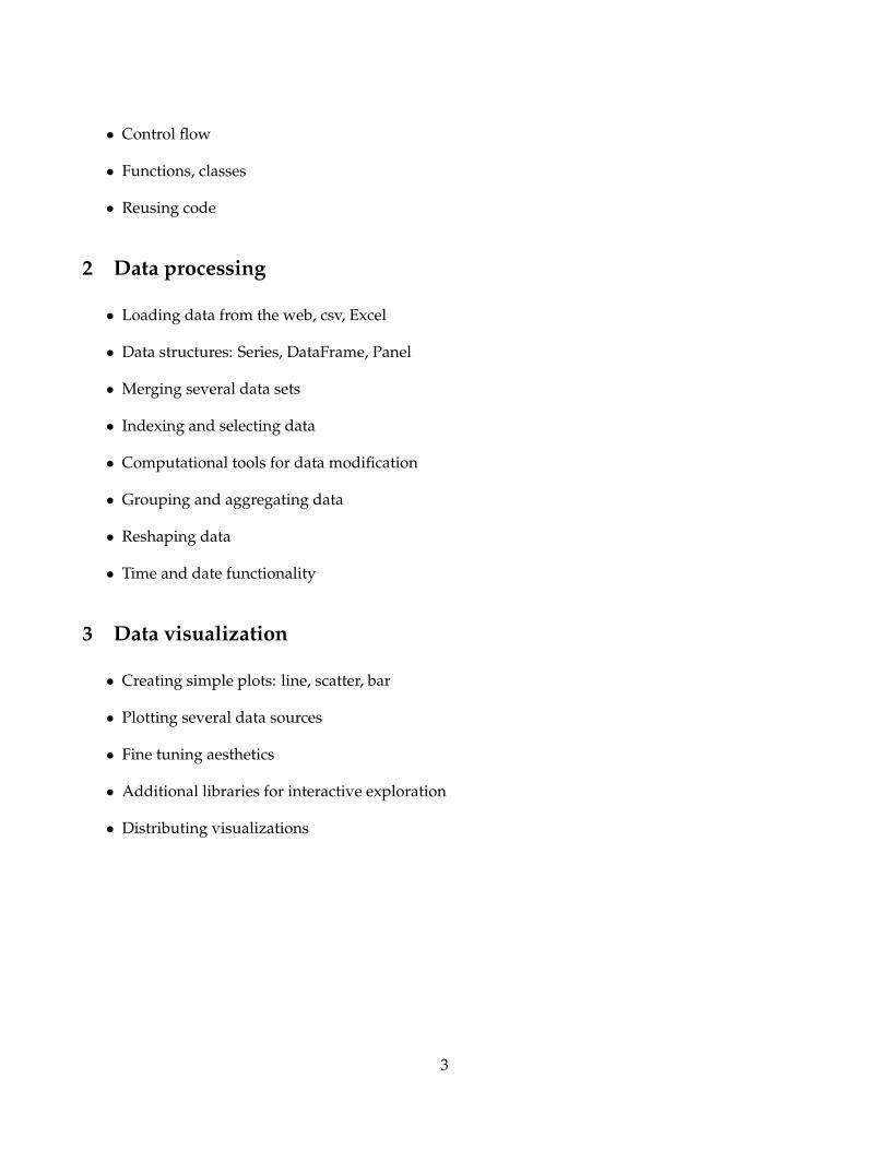
Q1.4 (5 points)Load 'id variables' sheet from the Excel file into Pandas DataFrame.Set 'id' variable as an index column.Convert all capital letters to lower case in all column names.Replace all missing values with integer '­999'.Covert all non­object columns to integers.Print shape of the dataset, column types, and first five rows.

The result of this question is saved in 'exam_data.hdf' under 'idvars' key.

In [5]:

(108, 8) ter int64 region_eng object rayon int64 fedokrug int64 fed_id int64 row_fed int64 row_rayon int64 region_rus object dtype: object ter region_eng rayon fedokrug fed_id row_fed \ id 1000 -999 Russian Federation -999 -999 0 1 1001 -999 Central Federal Okrug -999 -999 1 2 31 1114 Belgorod oblast 105 1001 101 3 32 1115 Bryansk oblast 103 1001 102 4 33 1117 Vladimir oblast 103 1001 103 5

row_rayon region_rus id 1000 1 Российская федерация 1001 -999 Центральный федеральный округ 31 35 Белгородская область 32 15 Брянская область 33 16 Владимирская область

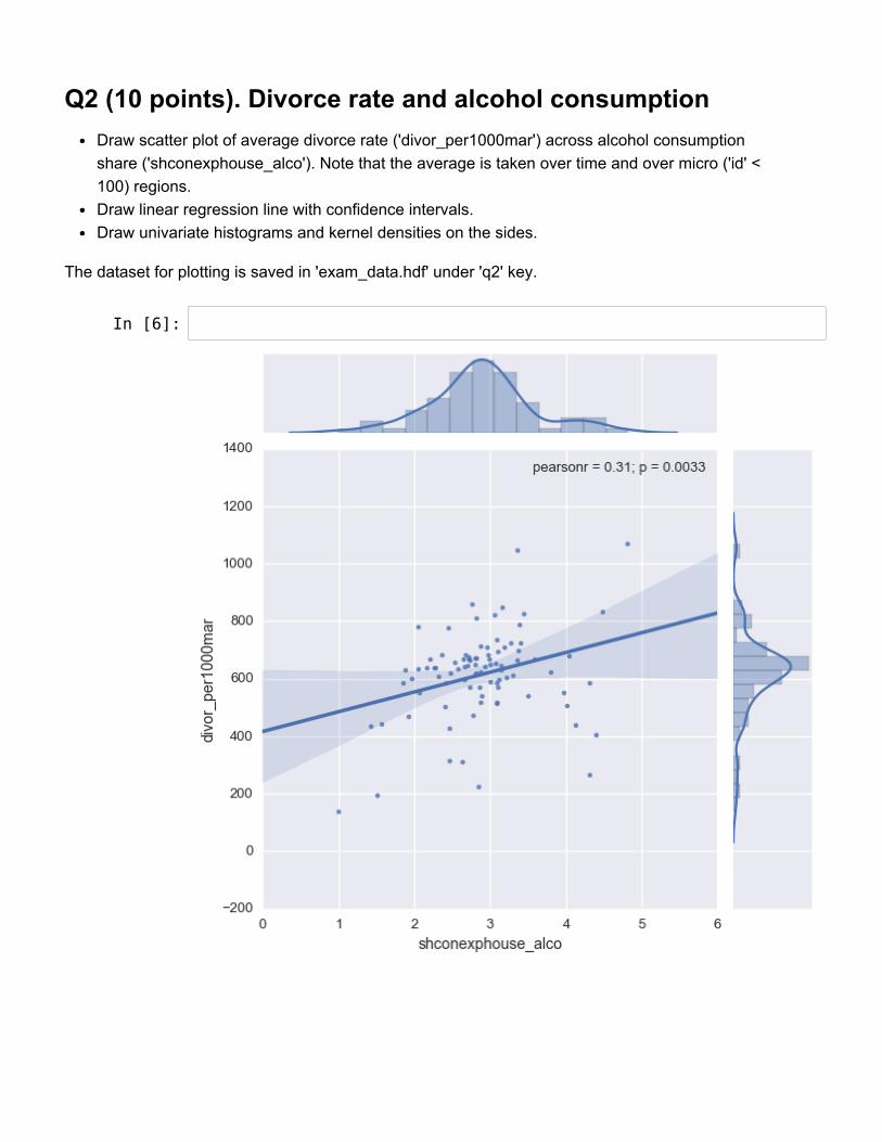
Q2 (10 points). Divorce rate and alcohol consumptionDraw scatter plot of average divorce rate ('divor_per1000mar') across alcohol consumptionshare ('shconexphouse_alco'). Note that the average is taken over time and over micro ('id' <100) regions.Draw linear regression line with confidence intervals.Draw univariate histograms and kernel densities on the sides.

The dataset for plotting is saved in 'exam_data.hdf' under 'q2' key.

In [6]:

Q3 (15 points). Birth rate and climate.Draw scatter plots of average birth rate ('birthcoeff') across average July and Januarytempreatures ('avertemp_jul', 'avertemp_jan'). Note that the average is taken over time and overmicro ('id' < 100) regions. Leave only data on micro regions ('id' < 100).Sort corresponding data by birth rate. Print first five and last five observations in one table.

The dataset for plotting is saved in 'exam_data.hdf' under 'q3' key.

In [7]:

region_eng St. Petersburg city 7.52 Tula oblast 7.60 Moskow oblast 7.71 Leningrad oblast 7.73 Ivanovo oblast 8.06 o/w Aginsk Buryat autonomous okrug 16.93 Tuva republic 19.19 Ingush republic 19.73 Dagestan republic 20.62 Chechnya republic 23.93 Name: birthcoeff, dtype: float64

Q4 (20 points). Unemployment and divorcePlot average unemployment level ('unempl_level') and divorce rate ('divor_per1000mar') foreach federal macro region ('fedokrug') over time ('year'). Note that the averaging is doneacross micro regions inside each macroregion ('id' > 1000). Leave only years from 1994 up to2003.Save the plot in pdf format.

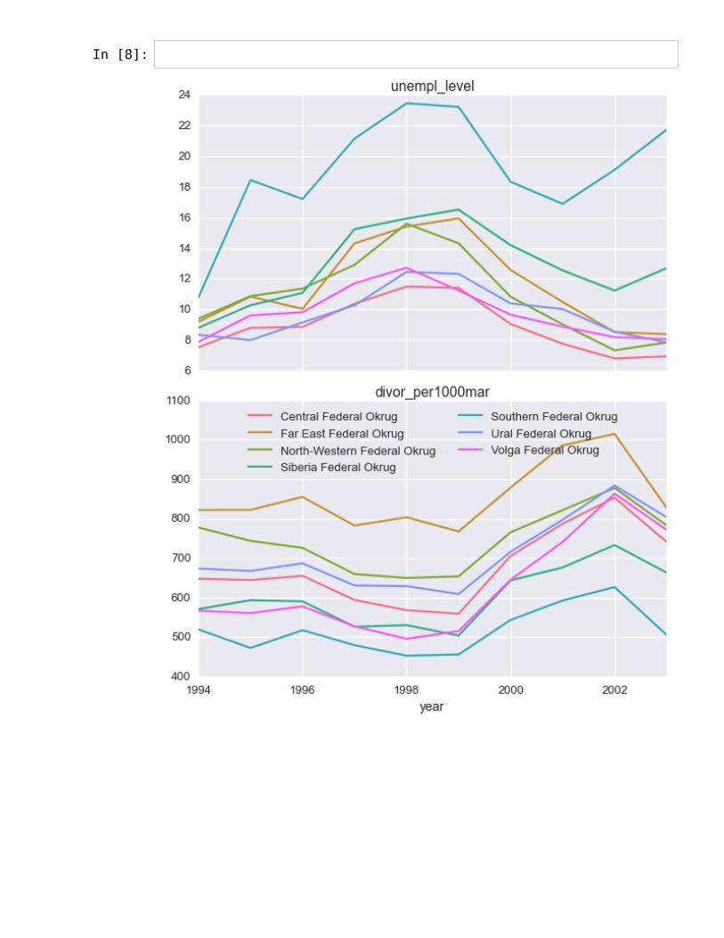
In [8]:

Q5. Changes in employment compositionDraw standard deviation of employment share by industry and macro region ('id' > 1000) across time.

Q5.1 (10 points)Create MultiIndex from 'id' and 'year'.Leave only those columns that start with 'shaaempl_'.Remove 'shaaempl_' from column names.Pivot DataFrame into Series called 'shaaempl' such that MultiIndex has another level called'industry'.Print first five rows.

The result is saved in 'exam_data.hdf' under 'q51' key.

In [9]:

id year industry 1000 1995-01-01 indus 25.80 agri 14.70 forest 0.40 constr 9.30 trans 6.60Name: shaaempl, dtype: float64

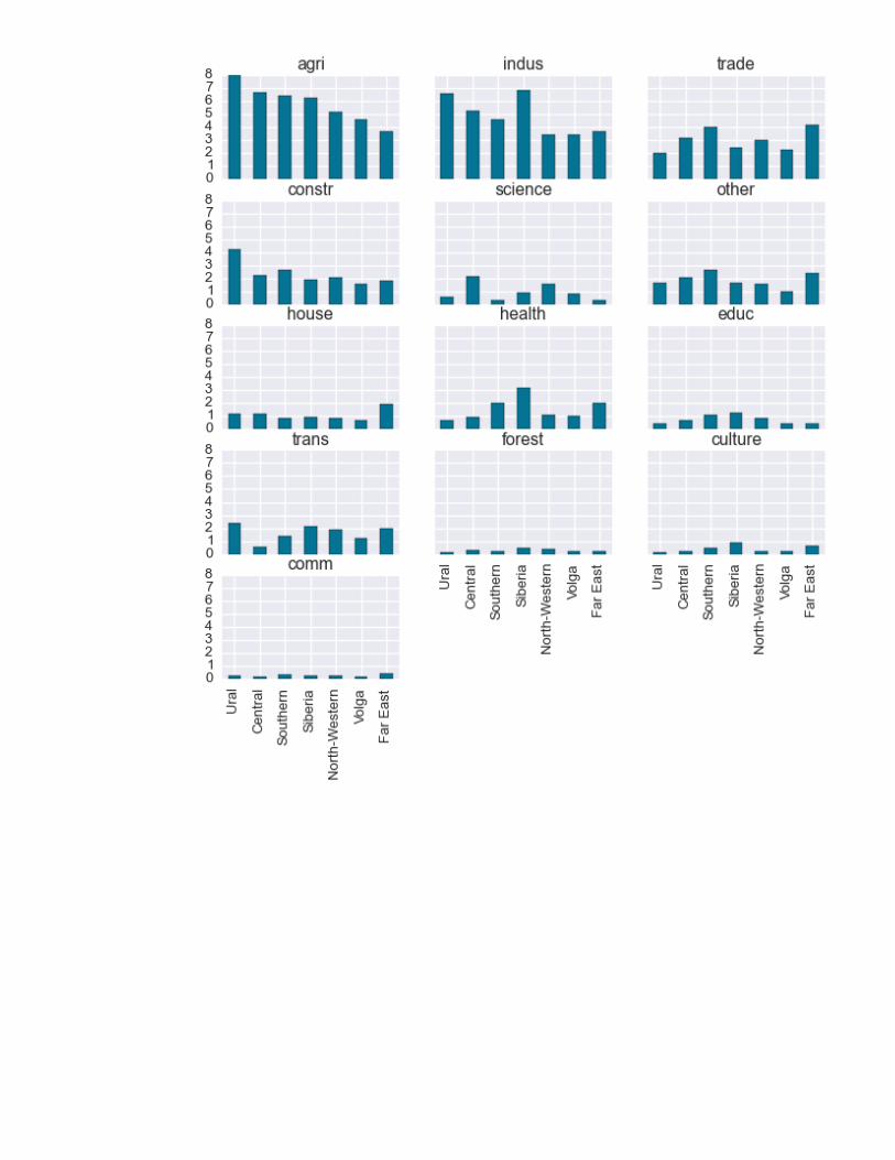
Q5.2 (30 points)Merge the data with 'idvars'.Compute standard deviation of employment share across all micro regions by federal macroregion ('id' > 1000) and by industry.Merge the result with 'idvars' again to obtain names of macro regions instead of their ids.Pivot DataFrame so that it has regions in rows and industries in columns.Remove ' Federal Okrug' from the name of a region.Sort rows 'agri' column.Sort columns by 'Central' region.Save the result as Excel and HTML file with two digits after the dot.Print first five rows.Draw bar plot.

The data for plotting is saved in 'exam_data.hdf' under 'q52' key.

In [10]:

industry agri indus trade constr science other house health \ Ural 7.98 6.60 2.01 4.18 0.60 1.64 1.19 0.67 Central 6.65 5.30 3.17 2.22 2.11 2.04 1.17 0.92 Southern 6.42 4.58 4.05 2.67 0.31 2.62 0.87 2.04 Siberia 6.23 6.83 2.47 1.88 0.85 1.64 0.97 3.18 North-Western 5.15 3.47 3.04 2.03 1.57 1.56 0.83 1.08

industry educ trans forest culture comm Ural 0.44 2.42 0.17 0.14 0.22 Central 0.69 0.54 0.32 0.26 0.16 Southern 1.13 1.39 0.23 0.51 0.30 Siberia 1.27 2.10 0.48 0.86 0.23 North-Western 0.83 1.87 0.42 0.23 0.29