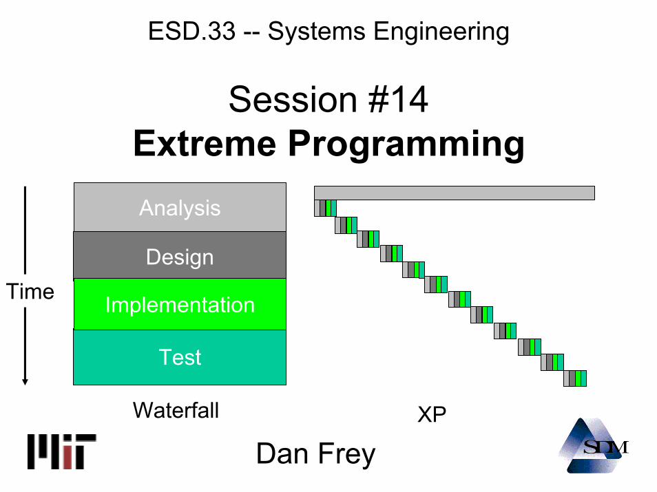
ESD.33 -- Systems Engineering

Session #14Extreme ProgrammingAnalysis

Test

Design

ImplementationTime

Waterfall XP

Dan Frey

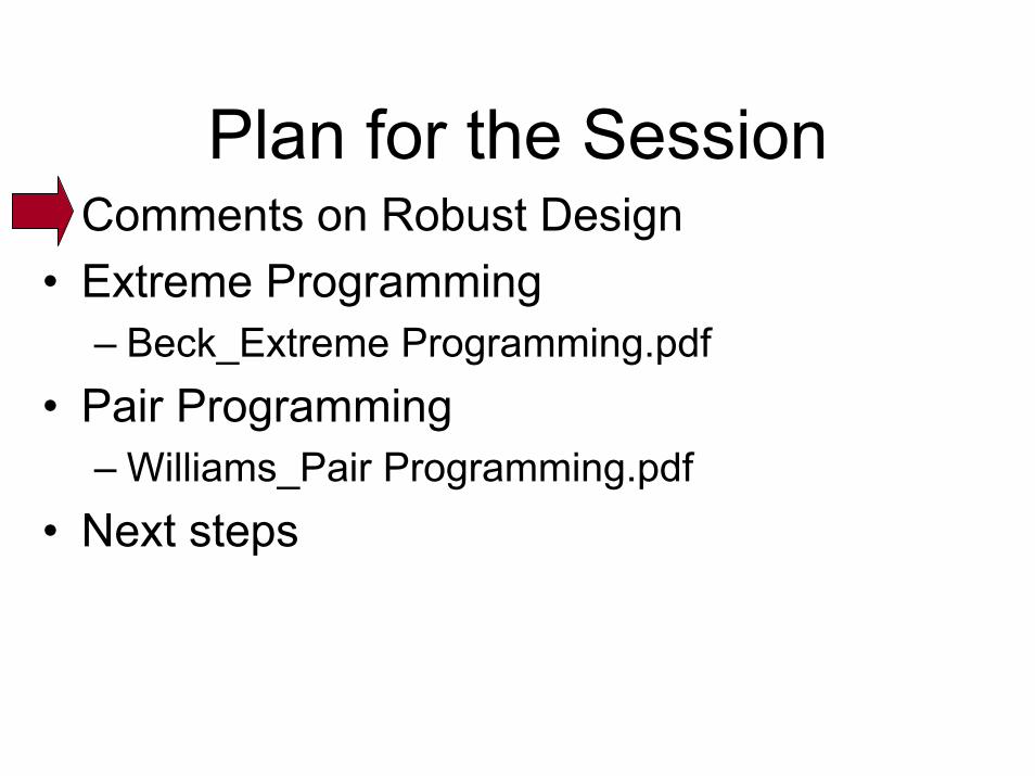
Plan for the Session• Comments on Robust Design• Extreme Programming

– Beck_Extreme Programming.pdf• Pair Programming

– Williams_Pair Programming.pdf• Next steps

Mal AthertonRolls-Royce, Controls Lead Engineer

I think a lot of students got lost towards the end today, because some of the details of the array types were difficult to cover in the short time we had.

Ari DimitriouChief Signal Processing Engineer, Raytheon

I was wondering if you could point me to more reading material on your DOE results. …

…a common Russian Submariner saying is "Better is the worst enemy of good enough". I feel the analysis you are making with OFAT may be supporting that argument...

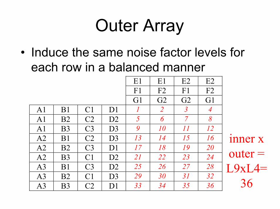
Outer Array• Induce the same noise factor levels for

each row in a balanced manner

inner xouter =L9xL4=

36

E1 E1 E2 E2F1 F2 F1 F2G1 G2 G2 G1

A1 B1 C1 D1 1 2 3 4A1 B2 C2 D2 5 6 7 8A1 B3 C3 D3 9 10 11 12A2 B1 C2 D3 13 14 15 16A2 B2 C3 D1 17 18 19 20A2 B3 C1 D2 21 22 23 24A3 B1 C3 D2 25 26 27 28A3 B2 C1 D3 29 30 31 32A3 B3 C2 D1 33 34 35 36

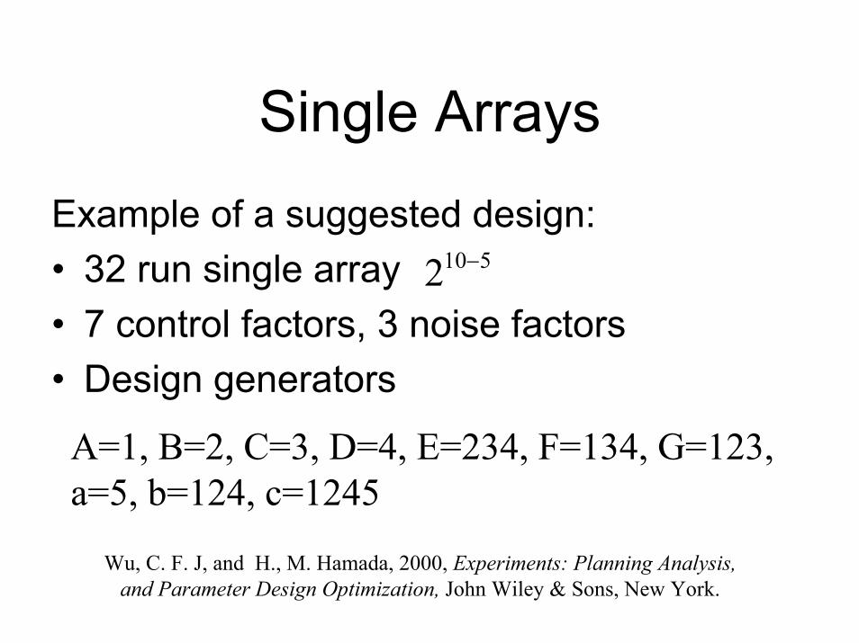
Single Arrays

5102 −

A=1, B=2, C=3, D=4, E=234, F=134, G=123, a=5, b=124, c=1245

Example of a suggested design:• 32 run single array• 7 control factors, 3 noise factors• Design generators

Wu, C. F. J, and H., M. Hamada, 2000, Experiments: Planning Analysis, and Parameter Design Optimization, John Wiley & Sons, New York.

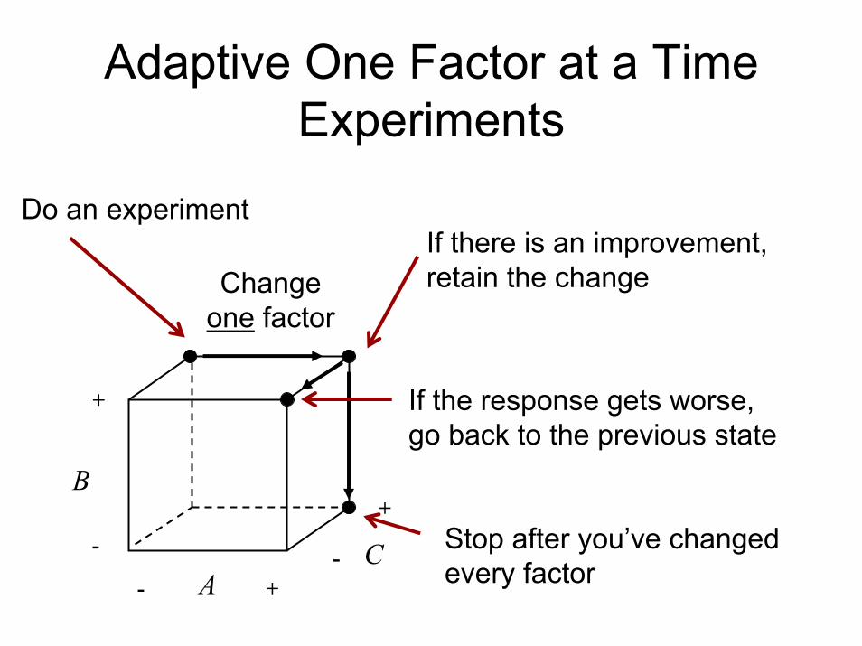
Adaptive One Factor at a Time Experiments

Do an experiment If there is an improvement, retain the changeChange

one factor

A

B

C

+

-

If the response gets worse, go back to the previous state

+

Stop after you’ve changed every factor

-

- +

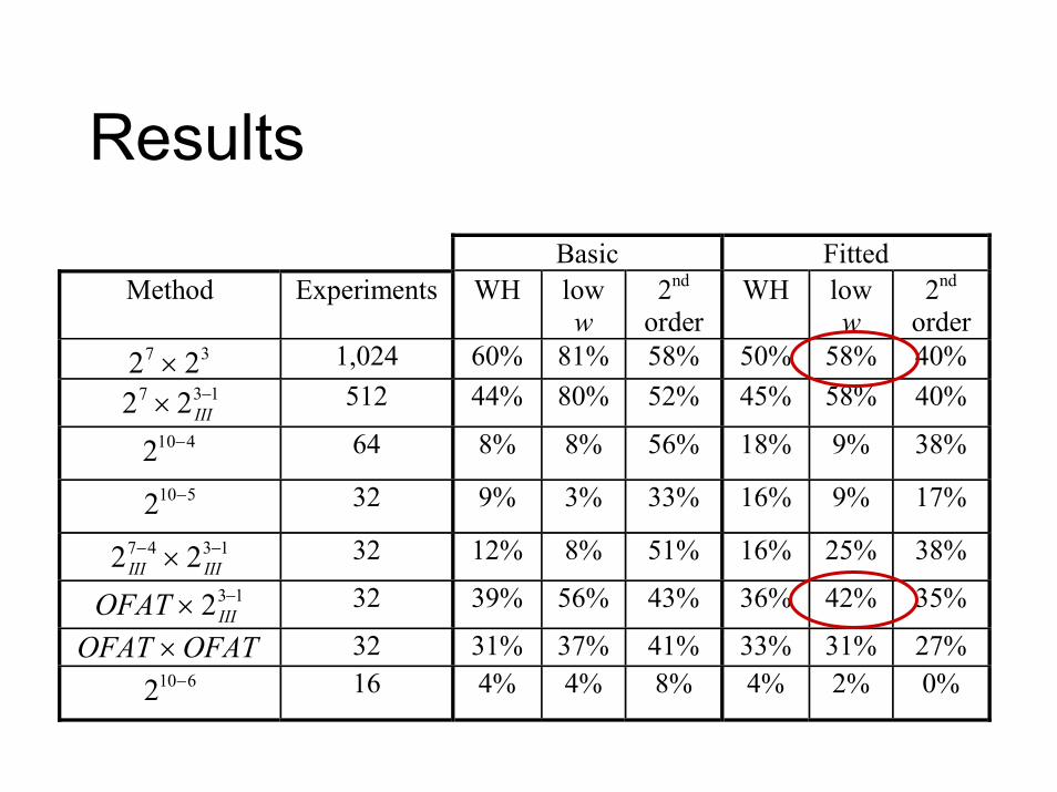
Results Basic Fitted

Method Experiments WH low w

2nd order

WH low w

2nd order

37 22 × 1,024 60% 81% 58% 50% 58% 40% 137 22 −× III 512 44% 80% 52% 45% 58% 40%

4102 − 64 8% 8% 56% 18% 9% 38%

5102 − 32 9% 3% 33% 16% 9% 17%

1347 22 −− × IIIIII 32 12% 8% 51% 16% 25% 38% 132 −× IIIOFAT 32 39% 56% 43% 36% 42% 35%

OFATOFAT × 32 31% 37% 41% 33% 31% 27% 6102 − 16 4% 4% 8% 4% 2% 0%

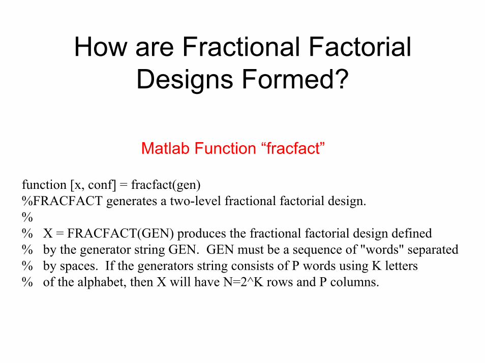
How are Fractional Factorial Designs Formed?

Matlab Function “fracfact”

function [x, conf] = fracfact(gen)%FRACFACT generates a two-level fractional factorial design.%% X = FRACFACT(GEN) produces the fractional factorial design defined% by the generator string GEN. GEN must be a sequence of "words" separated% by spaces. If the generators string consists of P words using K letters% of the alphabet, then X will have N=2^K rows and P columns.

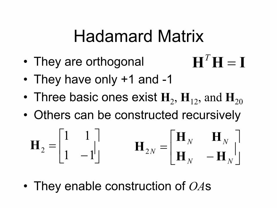
Hadamard Matrix• They are orthogonal• They have only +1 and -1• Three basic ones exist H2, H12, and H20

• Others can be constructed recursively

• They enable construction of OAs

⎥⎦

⎤⎢⎣

⎡−

=NN

NNN HH

HHH2

IHH =T

⎥⎦

⎤⎢⎣

⎡−

=11

112H

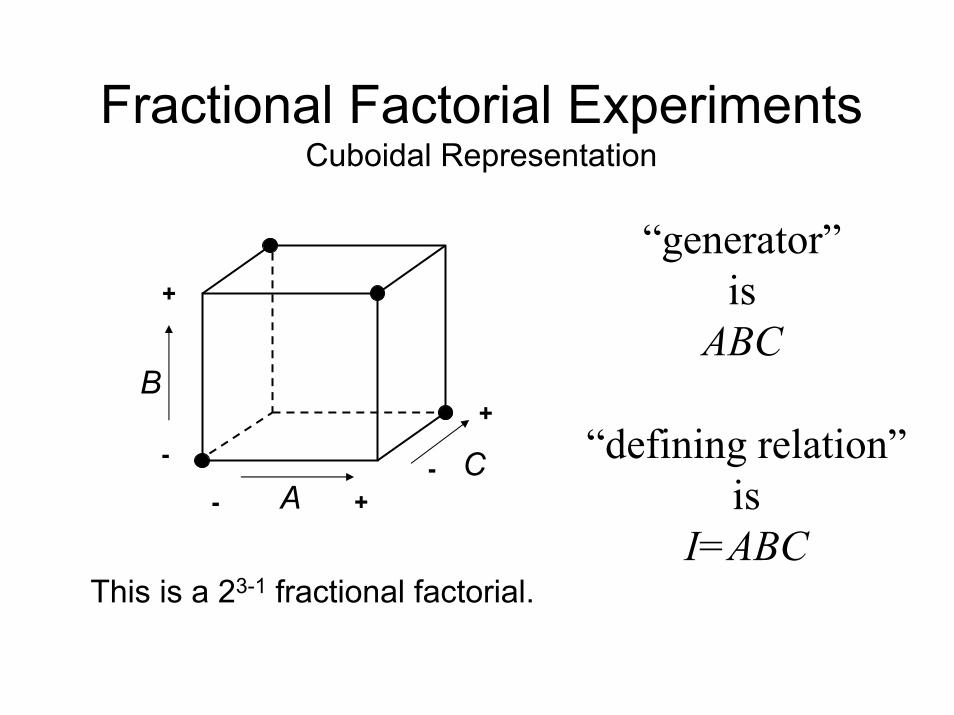
Fractional Factorial ExperimentsCuboidal Representation

“generator”is

ABC

AC

+

B

+

+

-“defining relation”

isI=ABC

-

-

This is a 23-1 fractional factorial.

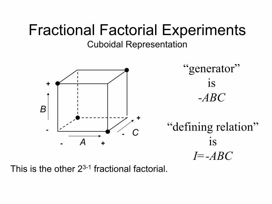
Fractional Factorial ExperimentsCuboidal Representation

“generator”is

-ABC

AC

+

B

+

+

--

-

This is the other 23-1 fractional factorial.

“defining relation”is

I=-ABC

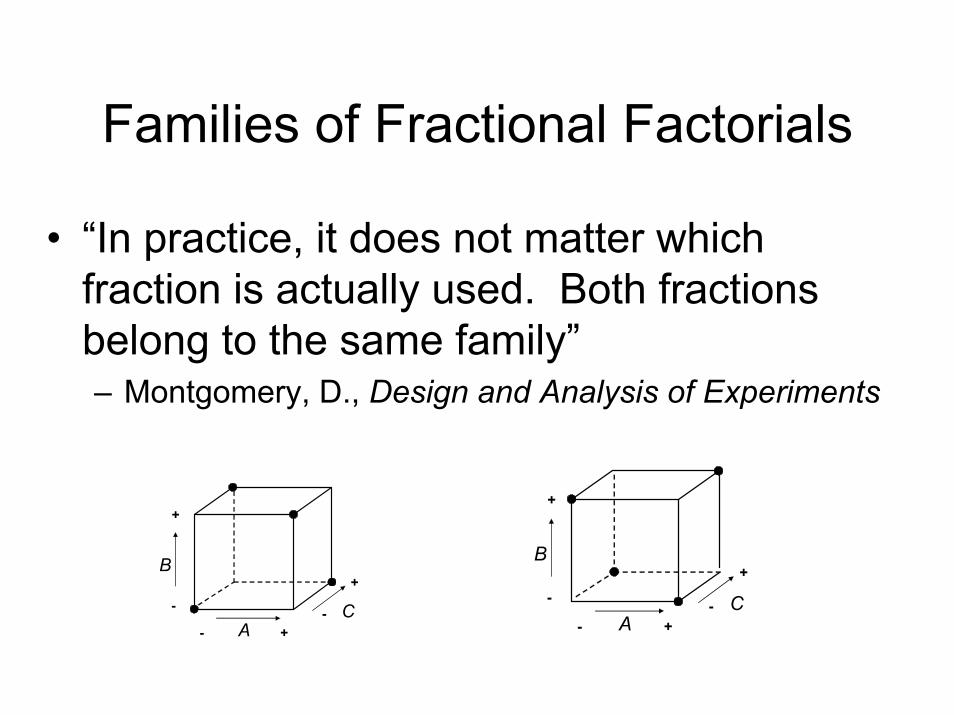
Families of Fractional Factorials

• “In practice, it does not matter which fraction is actually used. Both fractions belong to the same family”– Montgomery, D., Design and Analysis of Experiments

A

B

C

+

-

+

+

--

A

B

C

+

-

+

+

--

John ArrudaHamilton Sundstrand Engine Systems

Manager - Engine Control Systems & Flight Test Group

• You stated during the lecture that the order of the Control Factors on slide 20 made a difference and that this would result in different tests being conducted. I agree with that. ... What is the approach for deciding which permutation of the balanced orthogonal array to test or does it matter? …would the Factor Effect Plots generated as per slide 24 show the same information, i.e., identify those factors that generate the most improvement independent of which orthogonal array you ran for a given set of factors?

Greg AndriesPratt & Whitney, F135 TAD Validation Manager

A perfect P&W example of what Dr. Frey is talking about would be cruise TSFC optimization. There are a number of factors that could be changed to a given engine cycle that could contribute to a reduction in TSFC. … software scheduling changes of variable geometry … turbine flow area change … aero improvement to the compression system...

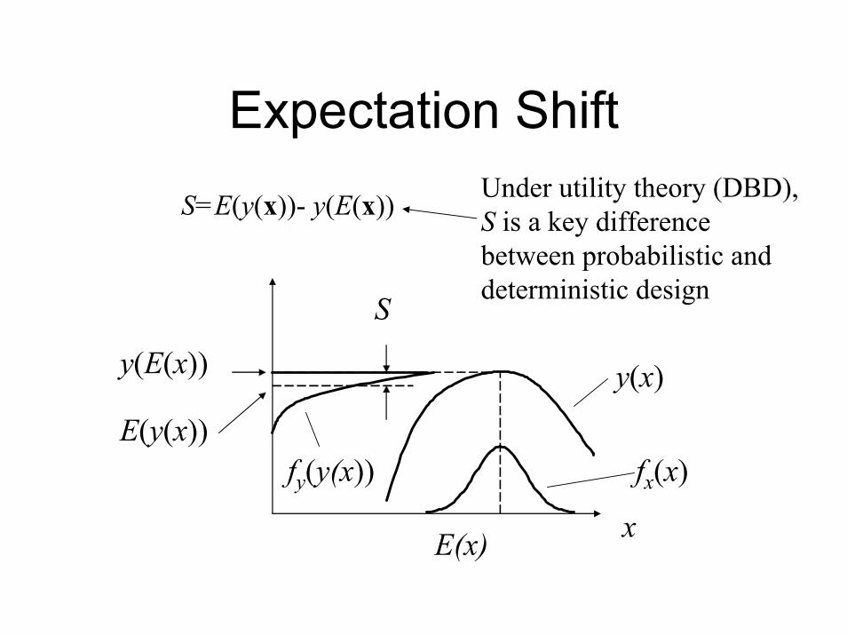
Expectation Shift

x

y(x)

E(x)

y(E(x))

E(y(x))

S

fx(x)fy(y(x))

S=E(y(x))- y(E(x)) Under utility theory (DBD),S is a key differencebetween probabilistic and deterministic design

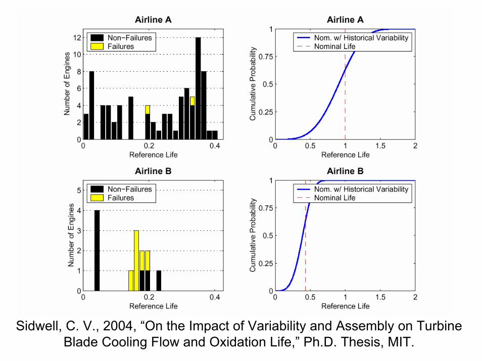
Sidwell, C. V., 2004, “On the Impact of Variability and Assembly on Turbine Blade Cooling Flow and Oxidation Life,” Ph.D. Thesis, MIT.

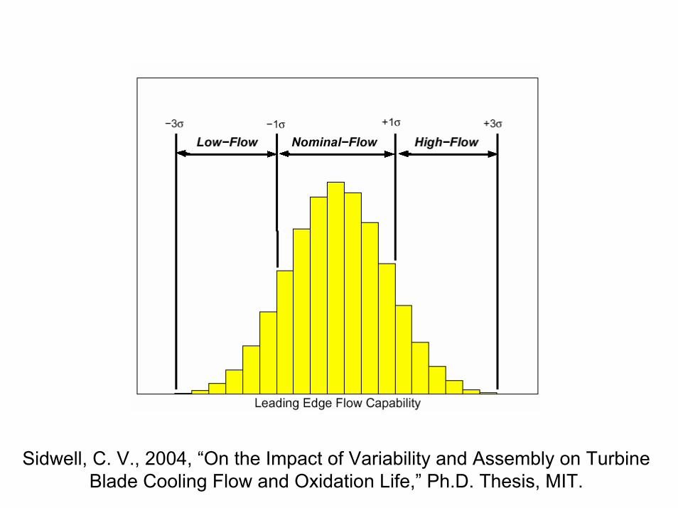
Sidwell, C. V., 2004, “On the Impact of Variability and Assembly on Turbine Blade Cooling Flow and Oxidation Life,” Ph.D. Thesis, MIT.

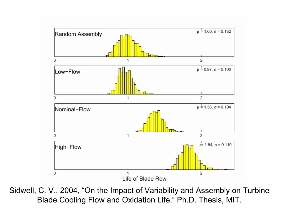
Sidwell, C. V., 2004, “On the Impact of Variability and Assembly on Turbine Blade Cooling Flow and Oxidation Life,” Ph.D. Thesis, MIT.

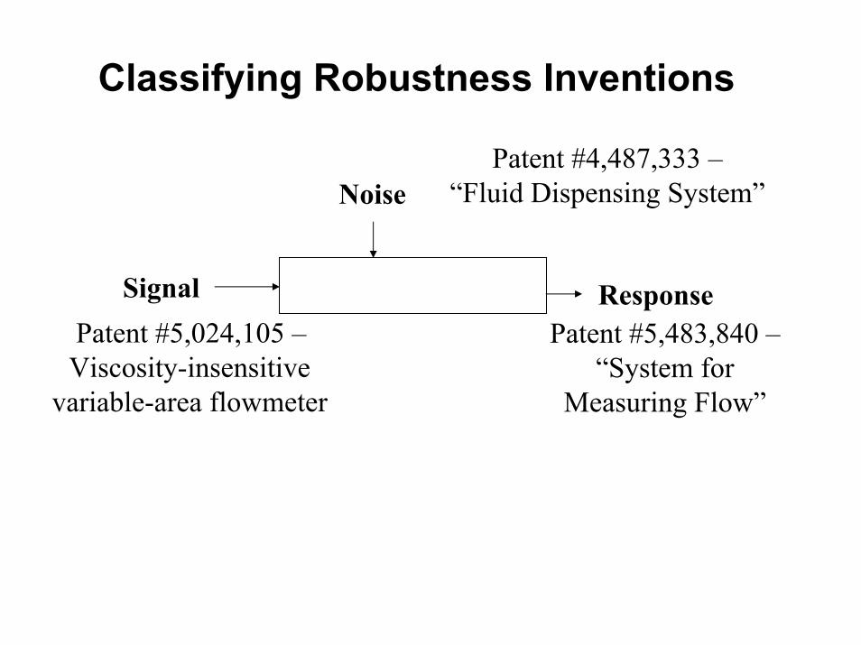
Classifying Robustness Inventions

Patent #4,487,333 –“Fluid Dispensing System”Noise

ResponseSignalPatent #5,024,105 –Viscosity-insensitive

variable-area flowmeter

Patent #5,483,840 –“System for

Measuring Flow”

Mal AthertonRolls-Royce, Controls Lead Engineer

In my experience, the main problem is the tendency to regard the spec (tolerance based) as the benchmark for all design decisions. We even have trouble convincing the company to allow us to perform robustness tests…Go fix the spec and stop asking for expensive and time consuming robustness tests we are told. … robustness is a design property that we should care about rather than just meeting the spec. Is this an appropriate way to view the issue?

History of Tolerances• pre 1800 -- Craft production systems• 1800 -- Invention of machine tools & the English

System of manufacture• 1850 -- Interchangeability of components & the

American system of manufacture

Jaikumar, Ramachandran, 1988, From Filing and Fitting to Flexible Manufacture

Craft Production• Drawings communicated rough proportion

and function• Drawings carried no specifications or

dimensions• Production involved the master, the model,

and calipers

The English System• Greater precision in machine tools• General purpose machines

– Maudslay invents the slide rest

• Accurate measuring instruments– Micrometers accurate to 0.001 inch

• Engineering drawings– Monge “La Geometrie Descriptive”– Orthographic views and dimensioning

• Parts made to fit to one another – Focus on perfection of fit

The American System

• Interchangeability required for field service of weapons

• Focus on management of clearances• Go-no go gauges employed to ensure fit• Allowed parts to be made in large lots

Go - no go gauges

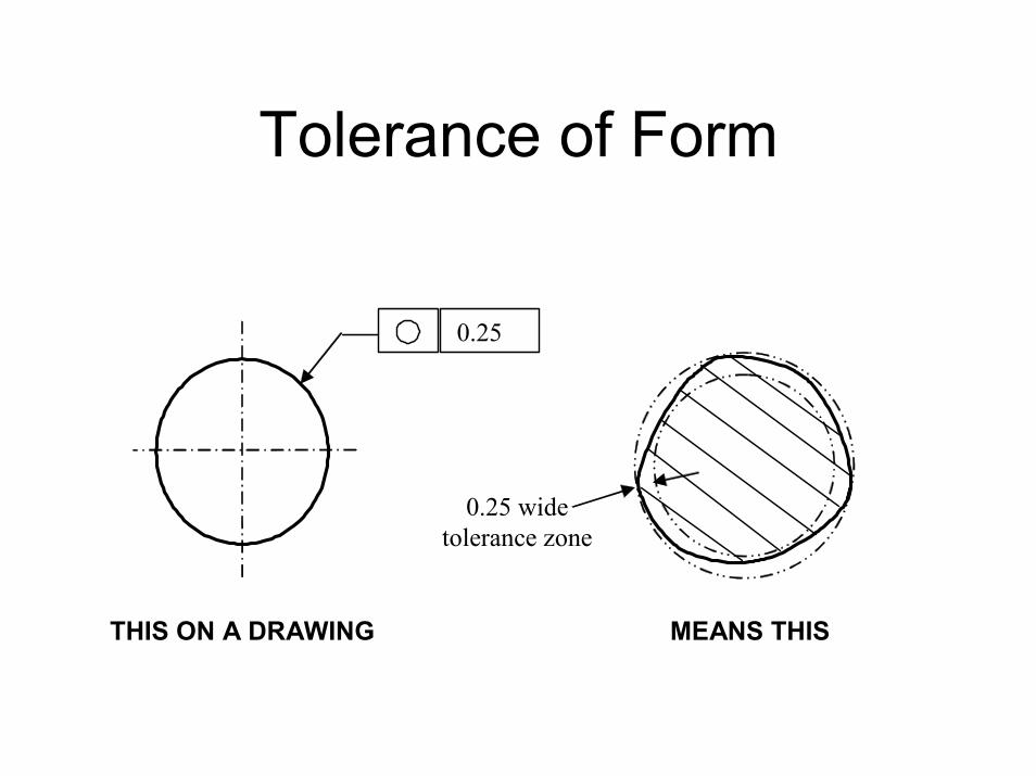
Tolerance of Form

0.25

THIS ON A DRAWING MEANS THIS

0.25 wide tolerance zone

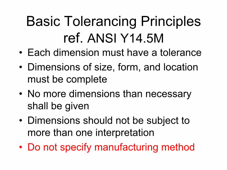
Basic Tolerancing Principlesref. ANSI Y14.5M

• Each dimension must have a tolerance• Dimensions of size, form, and location

must be complete• No more dimensions than necessary

shall be given• Dimensions should not be subject to

more than one interpretation• Do not specify manufacturing method

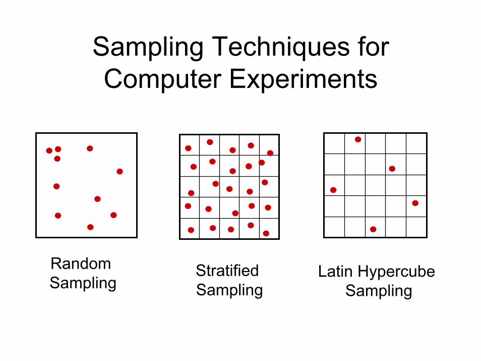
Sampling Techniques for Computer Experiments

Random Sampling

Stratified Sampling

Latin Hypercube Sampling

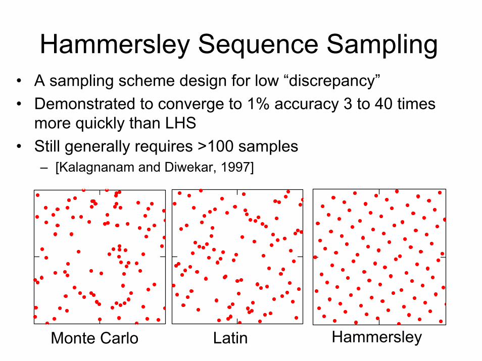
Hammersley Sequence Sampling• A sampling scheme design for low “discrepancy”• Demonstrated to converge to 1% accuracy 3 to 40 times

more quickly than LHS • Still generally requires >100 samples

– [Kalagnanam and Diwekar, 1997]

Monte Carlo Latin Hammersley

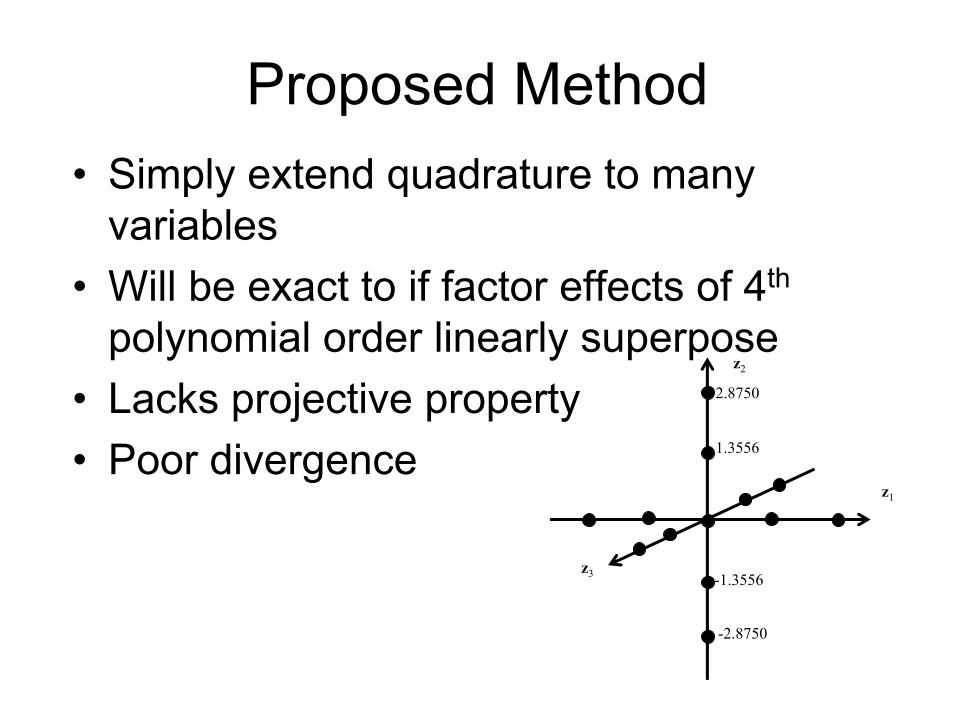
Proposed Method• Simply extend quadrature to many

variables• Will be exact to if factor effects of 4th

polynomial order linearly superpose• Lacks projective property• Poor divergence

z1

z2

z3

1.3556

2.8750

-1.3556

-2.8750

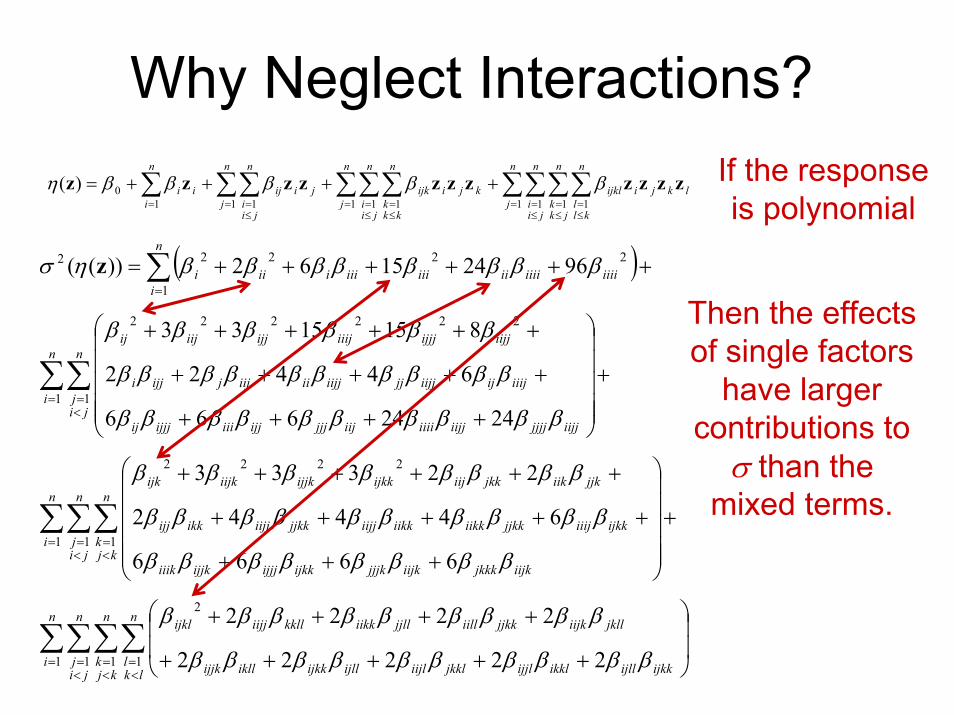
Why Neglect Interactions?If the response is polynomial

lk

n

j

n

jii

n

jkk

n

kll

jiijklk

n

j

n

jii

n

kkk

jiijkji

n

j

n

jii

ij

n

iii zzzzzzzzzzz ∑∑∑∑∑∑∑∑∑∑

=≤=

≤=

≤==

≤=

≤==

≤==

++++=1 1 1 11 1 11 11

0)( βββββη

( )

∑∑∑∑

∑∑∑

∑∑

∑

=<=

<=

<=

=<=

<=

=<=

=

⎟⎟

⎠

⎞

⎜⎜

⎝

⎛

+++++

++++

+

⎟⎟⎟⎟⎟

⎠

⎞

⎜⎜⎜⎜⎜

⎝

⎛

+++

+++++

++++++

+

⎟⎟⎟⎟⎟

⎠

⎞

⎜⎜⎜⎜⎜

⎝

⎛

++++

+++++

++++++

++++++=

n

i

n

jij

n

kjk

n

lkl ijkkijllikklijjljkkliijlijllijkkikllijjk

jklliijkjjkkiilljjlliikkkklliijjijkl

n

i

n

jij

n

kjk

iijkjkkkiijkjjjkijkkijjjijjkiiik

ijkkiiijjjkkiikkiikkiijjjjkkiijjikkijj

jjkiikjkkiijijkkijjkiijkijk

n

i

n

jij

iijjjjjjiijjiiiiiijjjjijjiiiijjjij

iiijijiijjjjiijjiiiijjijji

iijjijjjiiijijjiijij

n

iiiiiiiiiiiiiiiiiiiii

1 1 1 1

2

1 1 1

2222

1 1

222222

1

22222

22222

2222

6666

64442

22333

2424666

64422

8151533

96241562))((

ββββββββββ

βββββββββ

ββββββββ

ββββββββββ

ββββββββ

ββββββββββ

ββββββββββ

ββββββ

ββββββββησ z

Then the effects of single factors

have larger contributions to

σ than the mixed terms.

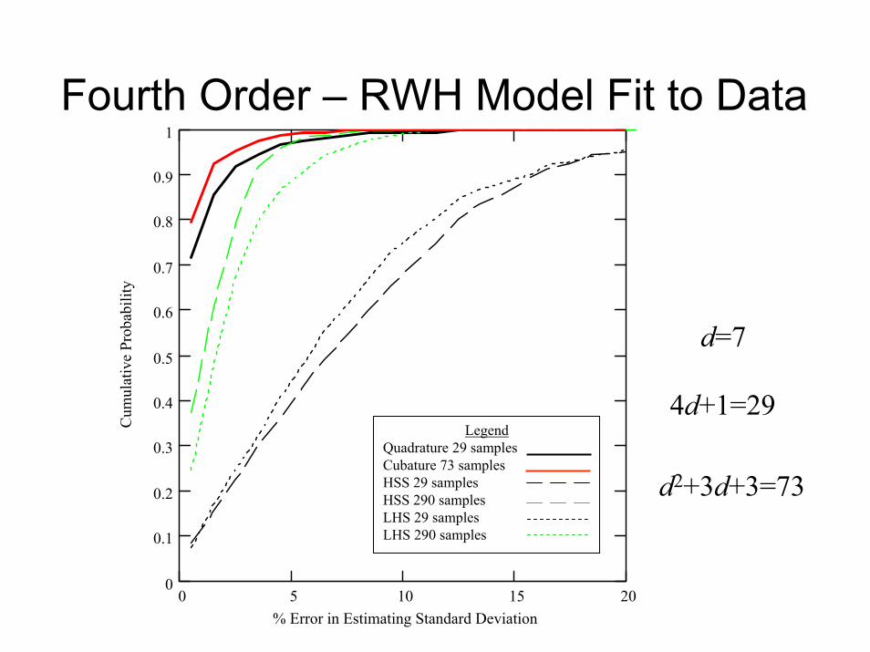
Fourth Order – RWH Model Fit to Data

LegendQuadrature 29 samplesCubature 73 samplesHSS 29 samplesHSS 290 samplesLHS 29 samplesLHS 290 samples

d=7

4d+1=29

d2+3d+3=73

0 5 10 15 200

0.1

0.2

0.3

0.4

0.5

0.6

0.7

0.8

0.9

1

% Error in Estimating Standard Deviation

Cum

ulat

ive

Prob

abili

ty

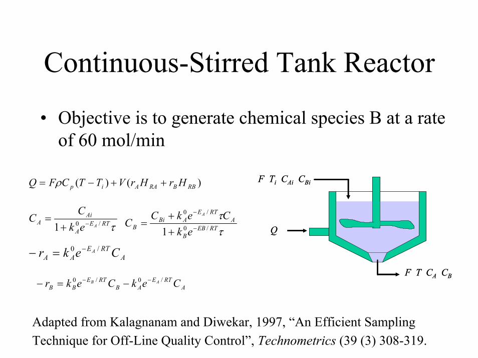
Continuous-Stirred Tank Reactor

• Objective is to generate chemical species B at a rate of 60 mol/min

)()( RBBRAAip HrHrVTTCFQ ++−= ρ

τRTEA

AiA Aek

CC /01 −+

=ττ

RTEBB

ARTE

ABiB ek

CekCC

A

/0

/0

1 −

−

++

=

ARTE

AA Cekr A /0 −=−

ARTE

ABRTE

BB CekCekr AB /0/0 −− −=−

Q

F Ti CAi CBi

F T CA CB

Q

F Ti CAi CBi

F T CA CB

Adapted from Kalagnanam and Diwekar, 1997, “An Efficient Sampling Technique for Off-Line Quality Control”, Technometrics (39 (3) 308-319.

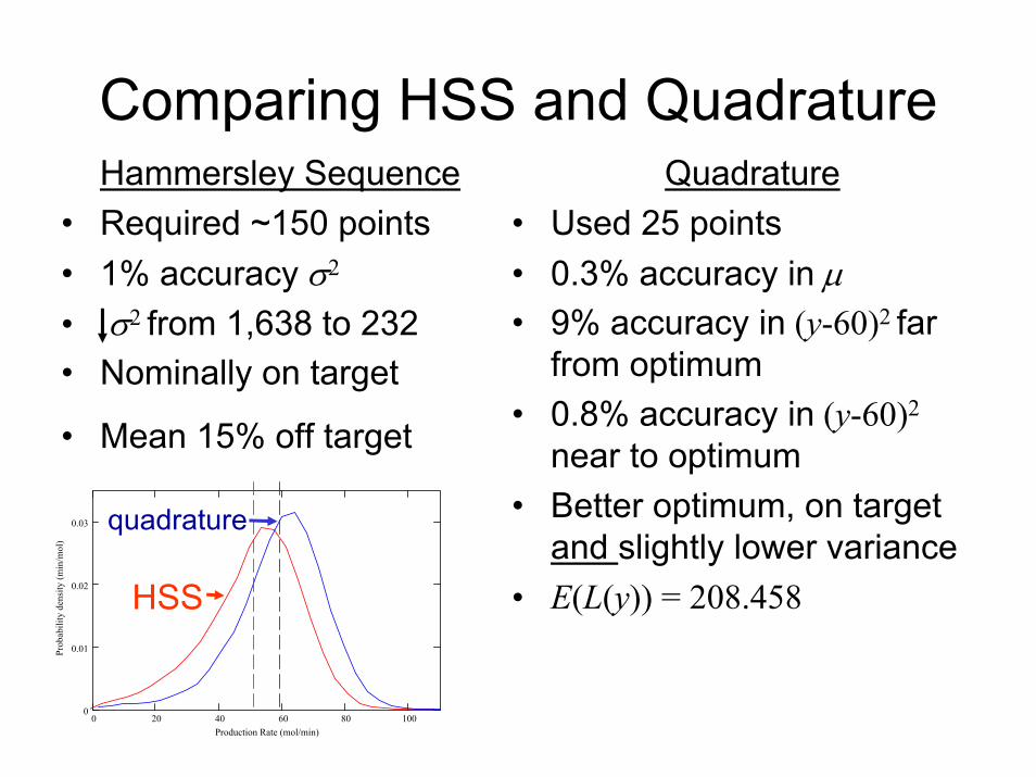
Comparing HSS and QuadratureHammersley Sequence

• Required ~150 points• 1% accuracy σ2

• σ2 from 1,638 to 232• Nominally on target

• Mean 15% off target

Quadrature• Used 25 points• 0.3% accuracy in µ• 9% accuracy in (y-60)2 far

from optimum• 0.8% accuracy in (y-60)2

near to optimum• Better optimum, on target

and slightly lower variance• E(L(y)) = 208.458

0

0.01

0.02

0.03

Prob

abili

ty d

ensi

ty (m

in/m

ol)

HSS

quadrature

0 20 40 60 80 100Production Rate (mol/min)

Plan for the Session• Comments on Robust Design• Extreme Programming

– Beck_Extreme Programming.pdf• Pair Programming

– Williams_Pair Programming.pdf• Next steps

Recap of “No Silver Bullet”

• What did Fred Brooks Say?• What is hard about software?• “Promising attacks on the conceptual

essence”– Buy versus build– Requirements refinement and rapid prototyping– Incremental development (grow, don’t build)– Great designers

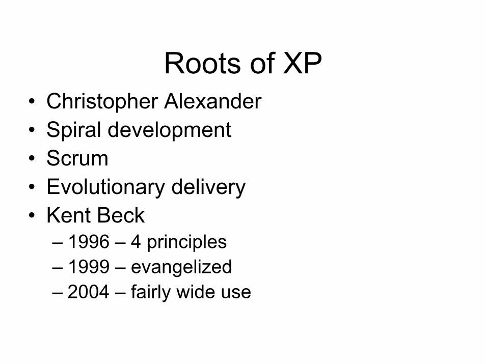
Roots of XP• Christopher Alexander• Spiral development• Scrum• Evolutionary delivery• Kent Beck

– 1996 – 4 principles– 1999 – evangelized– 2004 – fairly wide use

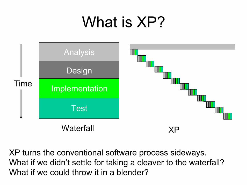
What is XP?

Analysis

Test

Design

ImplementationTime

Waterfall XP

XP turns the conventional software process sideways.What if we didn’t settle for taking a cleaver to the waterfall? What if we could throw it in a blender?

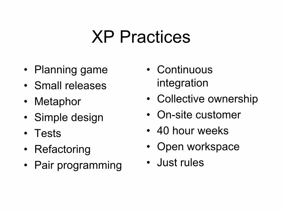
XP Practices

• Planning game• Small releases• Metaphor• Simple design• Tests• Refactoring• Pair programming

• Continuous integration

• Collective ownership• On-site customer• 40 hour weeks• Open workspace• Just rules

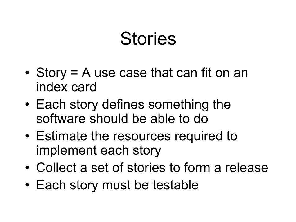
Stories

• Story = A use case that can fit on an index card

• Each story defines something the software should be able to do

• Estimate the resources required to implement each story

• Collect a set of stories to form a release• Each story must be testable

Unit Testing

• “If there is a technique at the heart of XP it is unit testing”

• Tests are what would convince the customer that the stories are completed

• Programmers write their OWN tests • Write the tests BEFORE the code• Test run automatically• Tests are permanent and accumulate

Pair Programming

• Programmers sign up for tasks for which they take responsibility for

• Responsible programmer finds a partner• The pair shares a single machine

– One person codes– The other critiques, helps, etc

• More later

Studies of Pair Progamming

• 15 experienced programmers, 5 individuals, 5 pairs – ~40% faster, higher quality [Nosek, 1998]

• 41 senior students, self selected to pair or individual programming – ~40-50% faster, more test cases passed [Williams, 2000]

• A good amount of anecdotal evidence from industry case studies

Other Arguments for Pair Programming

• Mistake avoidance – “two sets of eyes”• Programmers like it• If there is turn-over, you retain

knowledge• Facilitates learning from peers• Organizational unity

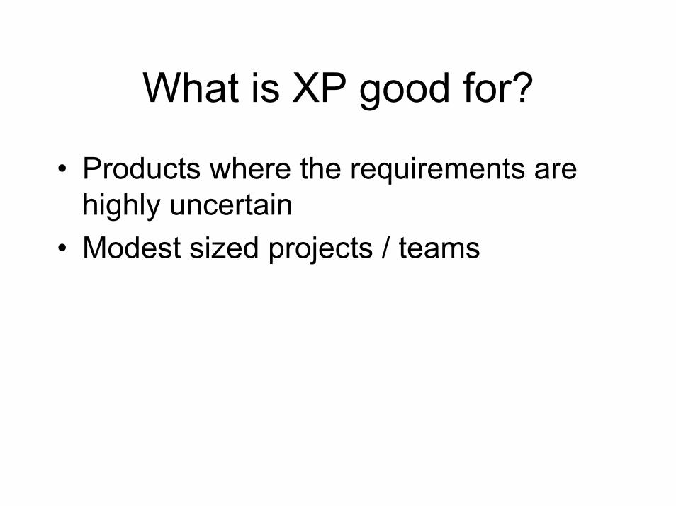
What is XP good for?

• Products where the requirements are highly uncertain

• Modest sized projects / teams

Other “Agile” Methods

• Scrum• XP • Crystal Orange• DSDM

Next Steps• Continue preparing for exam

– Exam posted next Tuesday AFTER session• See you at Tuesday’s session

– General Electric Aircraft Engine case study– 8:30AM Tuesday, 27 July

• Reading assignment– www.geae.com/education/engines101– Cumpsty_Jet Propulsion ch4.pdf