Embed Size (px)
Citation preview
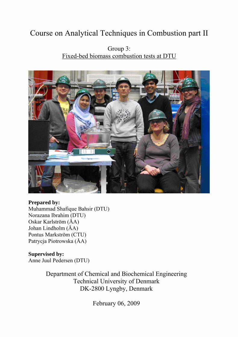
Course on Analytical Techniques in Combustion part II
Group 3: Fixed-bed biomass combustion tests at DTU
Prepared by: Muhammad Shafique Bahsir (DTU) Norazana Ibrahim (DTU) Oskar Karlström (ÅA) Johan Lindholm (ÅA) Pontus Markström (CTU) Patrycja Piotrowska (ÅA) Supervised by: Anne Juul Pedersen (DTU)
Department of Chemical and Biochemical Engineering Technical University of Denmark
DK-2800 Lyngby, Denmark
February 06, 2009
1 TABLE OF CONTENTS 1 TABLE OF CONTENTS.............................................................................................................2 2 INTRODUCTION .......................................................................................................................4 3 EXPERIMENTAL SET-UP ........................................................................................................5
3.1 Fuels .....................................................................................................................................5 3.2 Fixed-bed reactor .................................................................................................................6 3.3 Combustion tests ..................................................................................................................6
4 RESULTS AND DISCUSSION ..................................................................................................9 4.1 Theoretical flue gas calculations..........................................................................................9 4.2 Burnout time ......................................................................................................................10 4.3 Emission levels ..................................................................................................................17 4.4 Ash characterization...........................................................................................................19
5 CONCLUSIONS.........................................................................................................................22 6 REFERENCES...........................................................................................................................24
2
List of Figures Figure 1 Cynara cardunculus L. with the different parts to be investigated [1]..................................4 Figure 2 Proximate analyses of the investigated fuel samples............................................................5 Figure 3 Ultimate analysis of the investigated fuel samples................................................................5 Figure 4 Schematic drawing of the fixed-bed reactor at DTU.............................................................6 Figure 5 Time dependant flue gas compostion for Capitula at 600 °C..............................................12 Figure 6 Time dependant flue gas compostion for Capitula at 750 °C..............................................12 Figure 7 Time dependant flue gas compostion for Capitula at 900 °C..............................................13 Figure 8 Time dependant flue gas compostion for Leaves at 600 °C. ...............................................13 Figure 9 Time dependant flue gas compostion for Leaves at 750 °C. ...............................................14 Figure 10 Time dependant flue gas compostion for Leaves at 900 °C. .............................................14 Figure 11 Time dependant flue gas compostion for Stem at 600 °C. ................................................15 Figure 12 Time dependant flue gas compostion for Stem at 750 °C. ................................................15 Figure 13 Time dependant flue gas compostion for Stem at 900 °C. ................................................16 Figure 14 NO emission comparison at 600 °C. .................................................................................17 Figure 15 NO emission comparison at 750 °C. .................................................................................18 Figure 16 NO emission comparison at 900 °C. .................................................................................18 Figure 17 NO emissions for all investigated fuels at all temperatures. .............................................19 Figure 18 Elemental composition from SEM/EDX of ash samples (550ºC).....................................20 Figure 19 Elemental composition from SEM/EDX of ash samples (900ºC).....................................21 Figure 20 SEM/EDX spot analysis results for particle in ash from Stem (900ºC). ...........................21 Figure 21 SEM/EDX spot analysis for particle in ash from Leaves (900 ºC). ..................................22 Figure 22 SEM/EDX spopt analysis for particle in ash from Capitula (900 ºC). ..............................22 List of Tables Table 1 Experimental matrix................................................................................................................8 Table 2 Composition of stem and constituent representation ..............................................................9 Table 3 Flue gas composition for three samples at 600oC.................................................................10 Table 4 Flue gas composition for three samples at 750oC.................................................................10 Table 5 Flue gas composition for three samples at 900oC.................................................................10
3
2 INTRODUCTION
A fixed-bed setup at the CHEC Research Centre, Technical University of Denmark (DTU) is
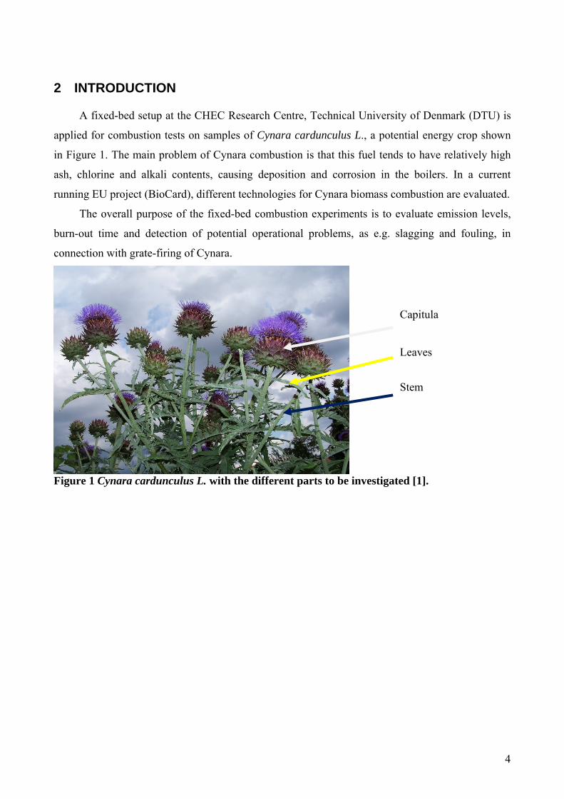
applied for combustion tests on samples of Cynara cardunculus L., a potential energy crop shown
in Figure 1. The main problem of Cynara combustion is that this fuel tends to have relatively high
ash, chlorine and alkali contents, causing deposition and corrosion in the boilers. In a current
running EU project (BioCard), different technologies for Cynara biomass combustion are evaluated.
The overall purpose of the fixed-bed combustion experiments is to evaluate emission levels,
burn-out time and detection of potential operational problems, as e.g. slagging and fouling, in
connection with grate-firing of Cynara.
Capitula
Leaves
Stem
Figure 1 Cynara cardunculus L. with the different parts to be investigated [1].
4
3 EXPERIMENTAL SET-UP
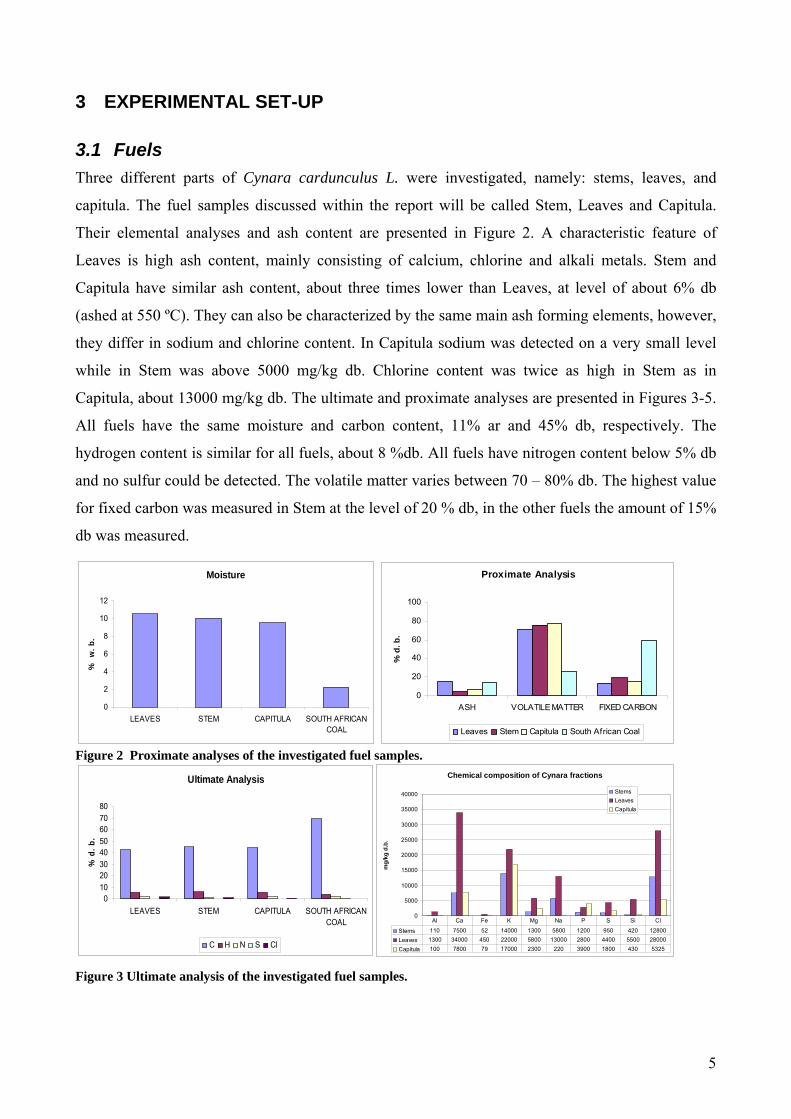
3.1 Fuels Three different parts of Cynara cardunculus L. were investigated, namely: stems, leaves, and
capitula. The fuel samples discussed within the report will be called Stem, Leaves and Capitula.
Their elemental analyses and ash content are presented in Figure 2. A characteristic feature of
Leaves is high ash content, mainly consisting of calcium, chlorine and alkali metals. Stem and
Capitula have similar ash content, about three times lower than Leaves, at level of about 6% db
(ashed at 550 ºC). They can also be characterized by the same main ash forming elements, however,
they differ in sodium and chlorine content. In Capitula sodium was detected on a very small level
while in Stem was above 5000 mg/kg db. Chlorine content was twice as high in Stem as in
Capitula, about 13000 mg/kg db. The ultimate and proximate analyses are presented in Figures 3-5.
All fuels have the same moisture and carbon content, 11% ar and 45% db, respectively. The
hydrogen content is similar for all fuels, about 8 %db. All fuels have nitrogen content below 5% db
and no sulfur could be detected. The volatile matter varies between 70 – 80% db. The highest value
for fixed carbon was measured in Stem at the level of 20 % db, in the other fuels the amount of 15%
db was measured.
Figure 2 Proximate analyses of the investigated fuel samples.
Figure 3 Ultimate analysis of the investigated fuel samples.
Moisture
0
2
4
6
8
10
12
LEAVES STEM CAPITULA SOUTH AFRICANCOAL
% w
. b.
Proximate Analysis
0
20
40
60
80
100
ASH VOLATILE MATTER FIXED CARBON
% d
. b.
Leaves Stem Capitula South African Coal
Ultimate Analysis
01020304050607080
LEAVES STEM CAPITULA SOUTH AFRICANCOAL
% d
. b.
C H N S Cl
Chemical composition of Cynara fractions
0
5000
10000
15000
20000
25000
30000
35000
40000
mg/
kg d
.b.
StemsLeavesCapitula
Stems 110 7500 52 14000 1300 5800 1200 950 420 12800Leaves 1300 34000 450 22000 5800 13000 2800 4400 5500 28000Capitula 100 7800 79 17000 2300 220 3900 1800 430 5325
Al Ca Fe K Mg Na P S Si Cl
5
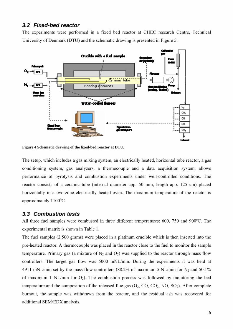
3.2 Fixed-bed reactor The experiments were performed in a fixed bed reactor at CHEC research Centre, Technical
University of Denmark (DTU) and the schematic drawing is presented in Figure 5.
Figure 4 Schematic drawing of the fixed-bed reactor at DTU.
The setup, which includes a gas mixing system, an electrically heated, horizontal tube reactor, a gas
conditioning system, gas analyzers, a thermocouple and a data acquisition system, allows
performance of pyrolysis and combustion experiments under well-controlled conditions. The
reactor consists of a ceramic tube (internal diameter app. 50 mm, length app. 125 cm) placed
horizontally in a two-zone electrically heated oven. The maximum temperature of the reactor is
approximately 1100oC.
3.3 Combustion tests All three fuel samples were combusted in three different temperatures: 600, 750 and 900ºC. The
experimental matrix is shown in Table 1.
The fuel samples (2.500 grams) were placed in a platinum crucible which is then inserted into the
pre-heated reactor. A thermocouple was placed in the reactor close to the fuel to monitor the sample
temperature. Primary gas (a mixture of N2 and O2) was supplied to the reactor through mass flow
controllers. The target gas flow was 5000 mNL/min. During the experiments it was held at
4911 mNL/min set by the mass flow controllers (88.2% of maximum 5 NL/min for N2 and 50.1%
of maximum 1 NL/min for O2). The combustion process was followed by monitoring the bed
temperature and the composition of the released flue gas (O2, CO, CO2, NO, SO2). After complete
burnout, the sample was withdrawn from the reactor, and the residual ash was recovered for
additional SEM/EDX analysis.
6

For the experiments performed at 900 and 750 ºC, the reactor was purged with N2 before the fuel
was inserted. When the sample was in position, the O2 valve was opened. At 600ºC the nitrogen and
oxygen flows were constant throughout the tests.
The combustion was considered finished when CO2 reached the 60 ppm level, and the sample was
taken out. The residual ash was weighed and stored for further analysis by SEM/EDX. The ash
contents in the different fuel fractions can be seen in Table 1. The excess air ratio was determined
according to equation 1, where the actual amount of oxygen is defined as the 10% O2 and the
minimum amount of oxygen is defined as the difference between the actual amount of air and
minimum O2 concentration in the flue gas during combustion.
7
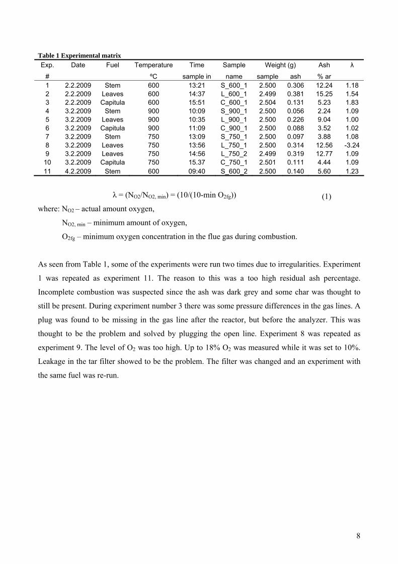
Table 1 Experimental matrix Exp. Date Fuel Temperature Time Sample Weight (g) Ash λ
# ºC sample in name sample ash % ar 1 2.2.2009 Stem 600 13:21 S_600_1 2.500 0.306 12.24 1.18 2 2.2.2009 Leaves 600 14:37 L_600_1 2.499 0.381 15.25 1.54 3 2.2.2009 Capitula 600 15:51 C_600_1 2.504 0.131 5.23 1.83 4 3.2.2009 Stem 900 10:09 S_900_1 2.500 0.056 2.24 1.09 5 3.2.2009 Leaves 900 10:35 L_900_1 2.500 0.226 9.04 1.00 6 3.2.2009 Capitula 900 11:09 C_900_1 2.500 0.088 3.52 1.02 7 3.2.2009 Stem 750 13:09 S_750_1 2.500 0.097 3.88 1.08 8 3.2.2009 Leaves 750 13:56 L_750_1 2.500 0.314 12.56 -3.24 9 3.2.2009 Leaves 750 14:56 L_750_2 2.499 0.319 12.77 1.09
10 3.2.2009 Capitula 750 15.37 C_750_1 2.501 0.111 4.44 1.09 11 4.2.2009 Stem 600 09:40 S_600_2 2.500 0.140 5.60 1.23
(1) λ = (N /N ) = (10/(10-min OO2 O2, min 2fg))
where: NO2 – actual amount oxygen,
N – minimum amount of oxygen, O2, min
O2fg – minimum oxygen concentration in the flue gas during combustion.
As seen from Table 1, some of the experiments were run two times due to irregularities. Experiment
1 was repeated as experiment 11. The reason to this was a too high residual ash percentage.
Incomplete combustion was suspected since the ash was dark grey and some char was thought to
still be present. During experiment number 3 there was some pressure differences in the gas lines. A
plug was found to be missing in the gas line after the reactor, but before the analyzer. This was
thought to be the problem and solved by plugging the open line. Experiment 8 was repeated as
experiment 9. The level of O was too high. Up to 18% O2 2 was measured while it was set to 10%.
Leakage in the tar filter showed to be the problem. The filter was changed and an experiment with
the same fuel was re-run.
8
4 RESULTS AND DISCUSSION
4.1 Theoretical flue gas calculations It is approximated that constituent representation of fuel on molar basis per kg will indicate the
approximate formula (molar composition) and ash in the fuel will act as inert. The composition of
stem is shown in Table 2.
Table 2 Composition of stem and constituent representation
Constituent Wt. (%) Constituent Representation
Mol. Wt.(g/mol) (Molar Composition)
C 47 12.00 α 35.606
β H 1.00 8 72.727 γ S 32.00 0 0.000
δN 14.00 1 0.649
φ O 16.00 36.8 20.909
ξ Cl 35.45 1.3 0.333
H2O 10 18.00 μ 5.051
Based on the strategy mentioned by [2], the approximate formula of the stem would
be . The chemical reaction can be written as
(approximated for products),
( )35.606 72.727 0.0 0.649 20.909 0.333 2 5.051C H S N O Cl H O⋅
( ) ( )35.606 72.727 0.0 0.649 20.909 0.333 2 25.051
2 2 2
C H S N O Cl H O +1.23 43.65O
35.606CO + 41.414H O +0.649NO+0.166Cl +10.0415O
⋅ ⋅
→
2
It is important to note that the above stoichiometric equation is based on the assumption that all the
available nitrogen in fuel will form NO. Now, using correlations mentioned by [2], the minimum
amount of oxygen and nitrogen required will be,
2 2
2
2 2 O +N ,mino
βα + 436.58mol4 2 2The minimum amount of (O +N ) = NX kgfuel
δ φγ+ + −= =
2 2FG,min O +N ,minβ δ φ 470.75molThe minimum amount of flue gas = N =N +α + +γ+ + =4 2 2 2 kgfuel
ξ+
( )2 2FG FG,min O +N ,min
571.17molThe amount of flue gas ( =1.18) = N =N + -1 Nkgfuel
λ λ =
9

The flue gas composition evaluated based on the correlations provided by [2] for each fuel and the
results are shown in Tables 3-5. oTable 3 Flue gas composition for three samples at 600 C.
Stem Leaves Capitula
Component Composition
CO2 0.0623 0.0492 0.0428 O2 0.0175 0.0334 0.0434
SO2 0 0 0 NO 0.0011 0,0019 0.0015 H2O 0,0725 0.0556 0.04914
oTable 4 Flue gas composition for three samples at 750 C
Stem Leaves Capitula
Component Composition
CO2 0.0704 0.0682 0.0699 O2 0.0069 0.0077 0.0077
SO2 0 0 0 NO 0.0012 0.0026 0.0025 H2O 0.0818 0.0771 0.0802
oTable 5 Flue gas composition for three samples at 900 C.
Stem Leaves Capitula
Component Composition
CO2 0.0698 0.0739 0.0744 O2 0.0077 0 0.0018
SO2 0 0 0 NO 0.0012 0.0029 0.0027 H2O 0.0811 0.0835 0.0853
4.2 Burnout time In the figures below CO, CO and O2 2 molar fractions in out-coming product gases from the
different Cyanara fractions are presented. The compete burn-out takes place when CO2
concentration is about 60 ppm and oxygen concentration reaches its initial value of 10 %.
Burn-out times at 600 °C
The burn-out time for Stem and Capitula are approximately 19 minutes, and the burn-out times for
Leaves is about 30 seconds shorter than in Stem and Capitula. The reason to the difference might be
due to the difference of the proximate analysis. Leaves, for example contains less volatile matter
and fixed carbon than Capitula and Stem. Another possible reason could be difference in char
oxidation reactivity.
10
Burn-out times at 750 °C
The burn-out time for Stem is approximately 12 minutes, the burn-out time for Capitula is 14
minutes and for Leaves about 12.5 minutes. The burn-out time for leaves is, again, the shortest. The
reason is the same as mentioned above. Another interesting feature with the CO and CO2 curves is
that in the beginning of the char conversion, the CO limit is close to zero. After some time, the CO
level increases, and in the end it again decreases. The CO level is zero at burn-out. A possible
reason could be that the char reactions take place further and further below the surface. Therefore,
there could be a lack of oxygen in the bottom of the char layer, that causes the formation of CO.
Burn-out times at 900 °C
The burn-out time for Stem is approximately 9.4 minutes, the burn-out time for Capitula is 10
minutes and Leaves is about 8.7 minutes. In the curves showing Stem and Leaves, the same CO
behavior as for the 750 °C curves can be observed.
Comparisons of the burn-out times at different temperatures
At 600 °C the burn-out times are 30 seconds different for the investigated fuels. At higher
temperatures, the difference between the burn-out times increases. A possible reason could be that
at the lower temperatures kinetics limits the char conversion. When the temperature increases the
mass transfer of oxygen becomes more important. If the diffusion of oxygen in the different chars
differs, the deviation between the different burn-out times could be explained.
11
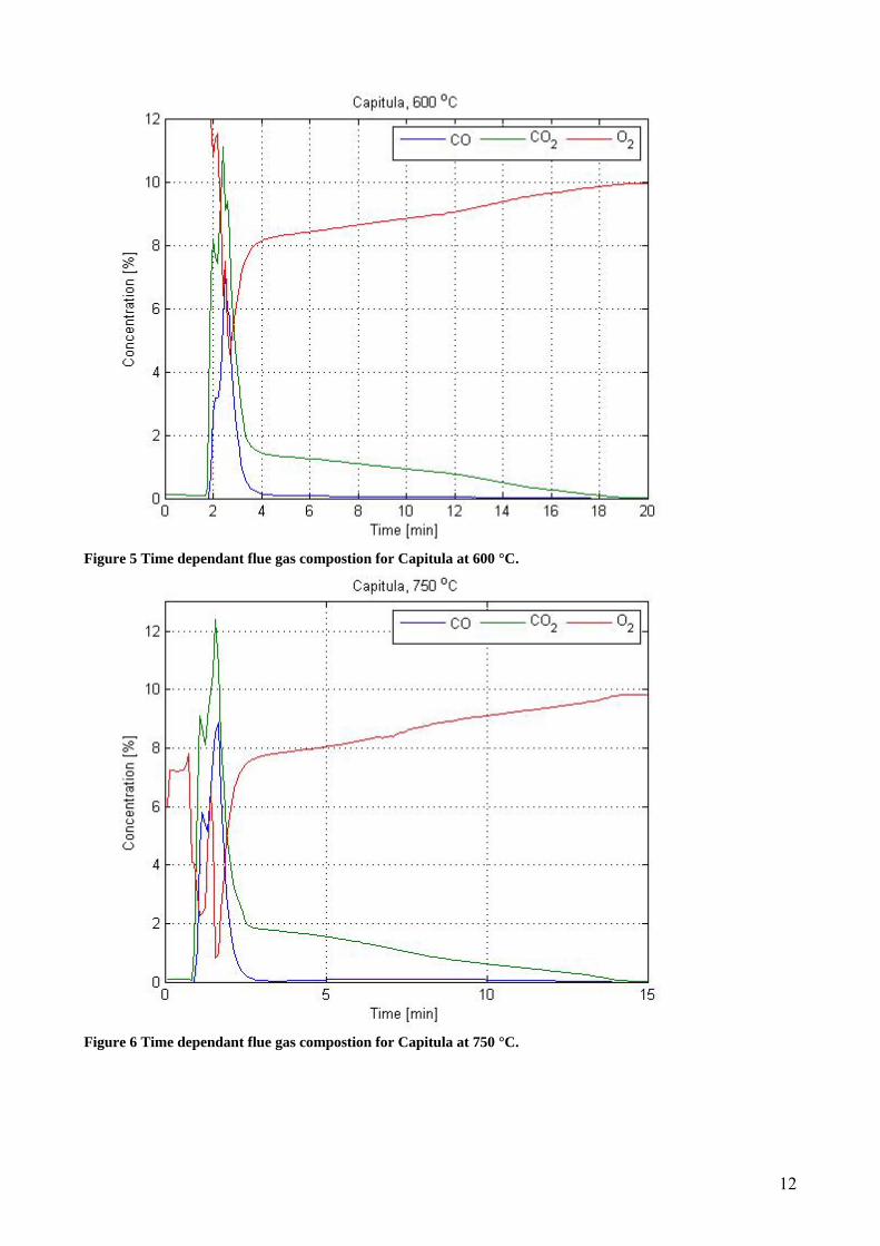
Figure 5 Time dependant flue gas compostion for Capitula at 600 °C.
Figure 6 Time dependant flue gas compostion for Capitula at 750 °C.
12

Figure 7 Time dependant flue gas compostion for Capitula at 900 °C.
Figure 8 Time dependant flue gas compostion for Leaves at 600 °C.
13
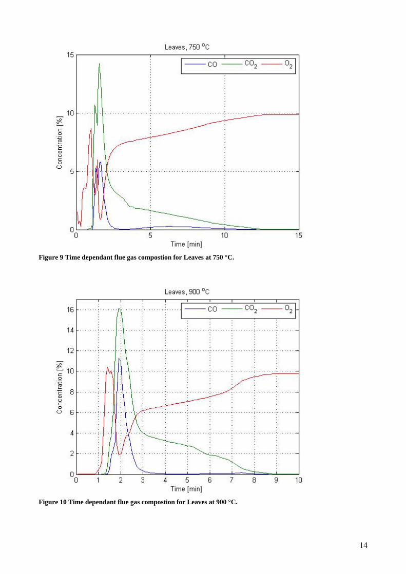
Figure 9 Time dependant flue gas compostion for Leaves at 750 °C.
Figure 10 Time dependant flue gas compostion for Leaves at 900 °C.
14
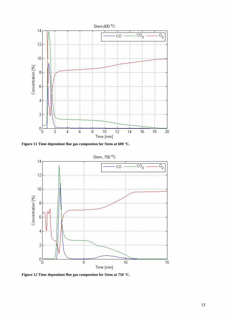
Figure 11 Time dependant flue gas compostion for Stem at 600 °C.
Figure 12 Time dependant flue gas compostion for Stem at 750 °C.
15
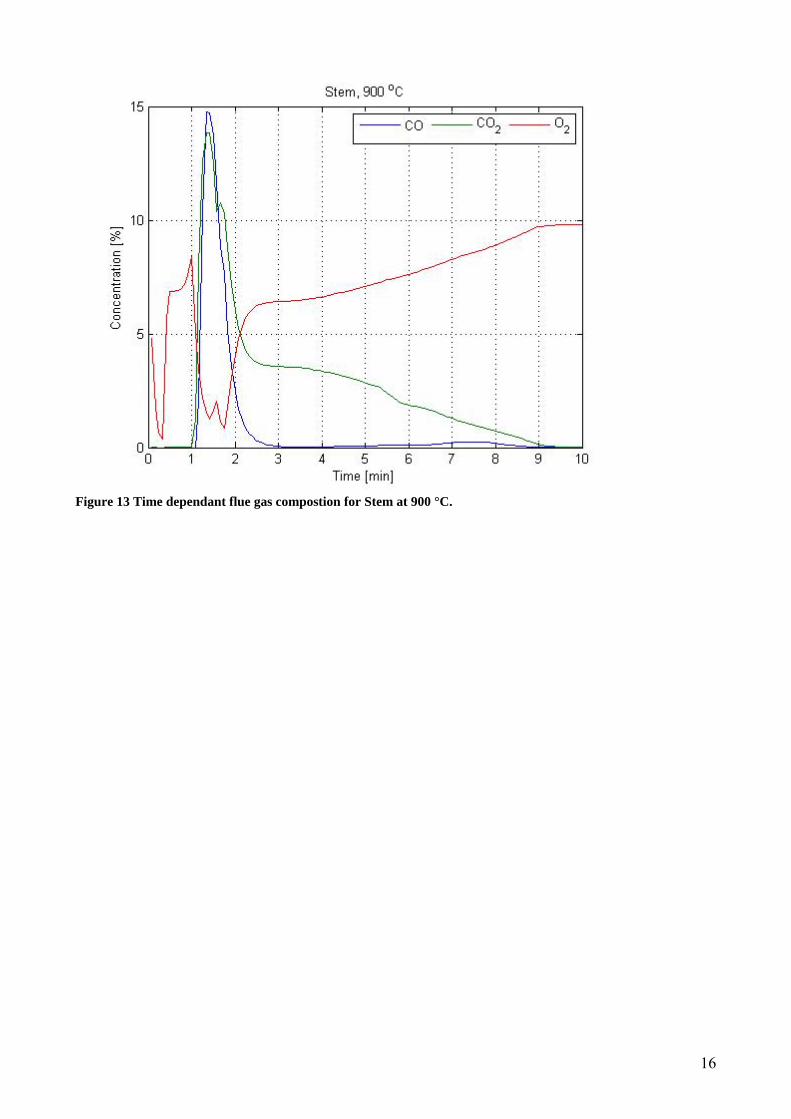
Figure 13 Time dependant flue gas compostion for Stem at 900 °C.
16
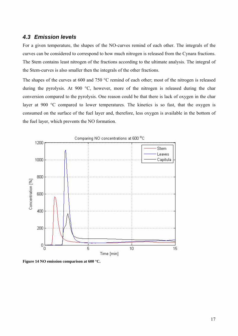
4.3 Emission levels For a given temperature, the shapes of the NO-curves remind of each other. The integrals of the
curves can be considered to correspond to how much nitrogen is released from the Cynara fractions.
The Stem contains least nitrogen of the fractions according to the ultimate analysis. The integral of
the Stem-curves is also smaller then the integrals of the other fractions.
The shapes of the curves at 600 and 750 °C remind of each other; most of the nitrogen is released
during the pyrolysis. At 900 °C, however, more of the nitrogen is released during the char
conversion compared to the pyrolysis. One reason could be that there is lack of oxygen in the char
layer at 900 °C compared to lower temperatures. The kinetics is so fast, that the oxygen is
consumed on the surface of the fuel layer and, therefore, less oxygen is available in the bottom of
the fuel layer, which prevents the NO formation.
Figure 14 NO emission comparison at 600 °C.
17

Figure 15 NO emission comparison at 750 °C.
Figure 16 NO emission comparison at 900 °C.
18

Figure 17 NO emissions for all investigated fuels at all temperatures.
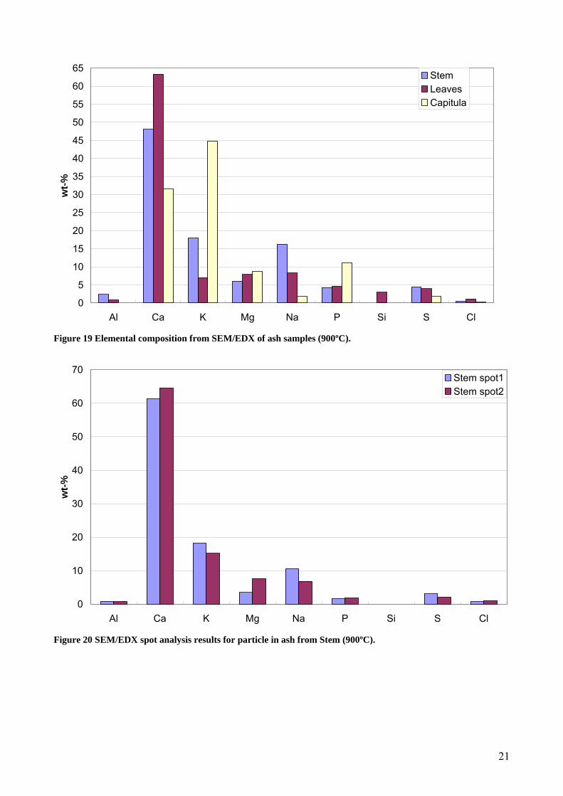
4.4 Ash characterization The composition of ash determined at 550 ºC for the investigated fuels from a previous study
is shown in Figure 18. The ash obtained in the end of each experiment was stored for SEM/EDX
analysis. Only the samples from the experiments at 900ºC of each fuel were analyzed. For that
purpose, the ash samples were mounted on an aluminum stub on which a carbon tape had been
placed. The overall analysis of ash samples were performed at 5 times magnification and are shown
in Figure 19.
The total ash content decreased with the temperature for all fuels (Figure 2, Table 1). This
could be due to volatile inorganic species present in the fuels. This is in agreement with the
elemental analysis (Figure 18 and Figure 19). The chlorine content in all samples has decreased
more than 5 times in the ash for all samples. Potassium content has decreased to about 50% for
Stem and Leaves. For the Capitula potassium content remained at the same level. In case of sodium
it has slightly decreased or remained constant in all investigated samples. Sulfur content in Capitula
has decreased to about 50% probably due to sulfur dioxide emissions. The sulfur emissions were
probably below the detection limit of the analyzer, and therefore they are not discussed in Emission
levels chapter. The sulfur has remained constant in the 900ºC ash for Stem and Leaves. The main
constituent of ash in all fuels is calcium followed by potassium. The calcium content trend in the
19
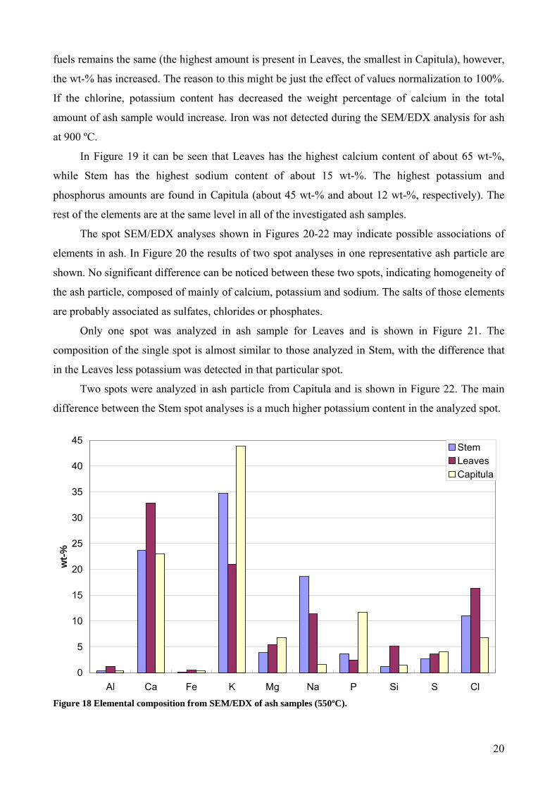
fuels remains the same (the highest amount is present in Leaves, the smallest in Capitula), however,
the wt-% has increased. The reason to this might be just the effect of values normalization to 100%.
If the chlorine, potassium content has decreased the weight percentage of calcium in the total
amount of ash sample would increase. Iron was not detected during the SEM/EDX analysis for ash
at 900 ºC.
In Figure 19 it can be seen that Leaves has the highest calcium content of about 65 wt-%,
while Stem has the highest sodium content of about 15 wt-%. The highest potassium and
phosphorus amounts are found in Capitula (about 45 wt-% and about 12 wt-%, respectively). The
rest of the elements are at the same level in all of the investigated ash samples.
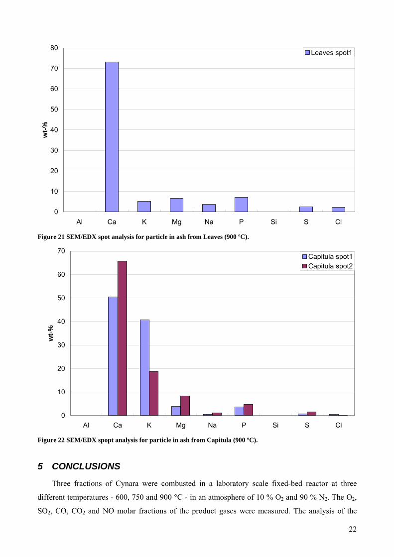
The spot SEM/EDX analyses shown in Figures 20-22 may indicate possible associations of
elements in ash. In Figure 20 the results of two spot analyses in one representative ash particle are
shown. No significant difference can be noticed between these two spots, indicating homogeneity of
the ash particle, composed of mainly of calcium, potassium and sodium. The salts of those elements
are probably associated as sulfates, chlorides or phosphates.
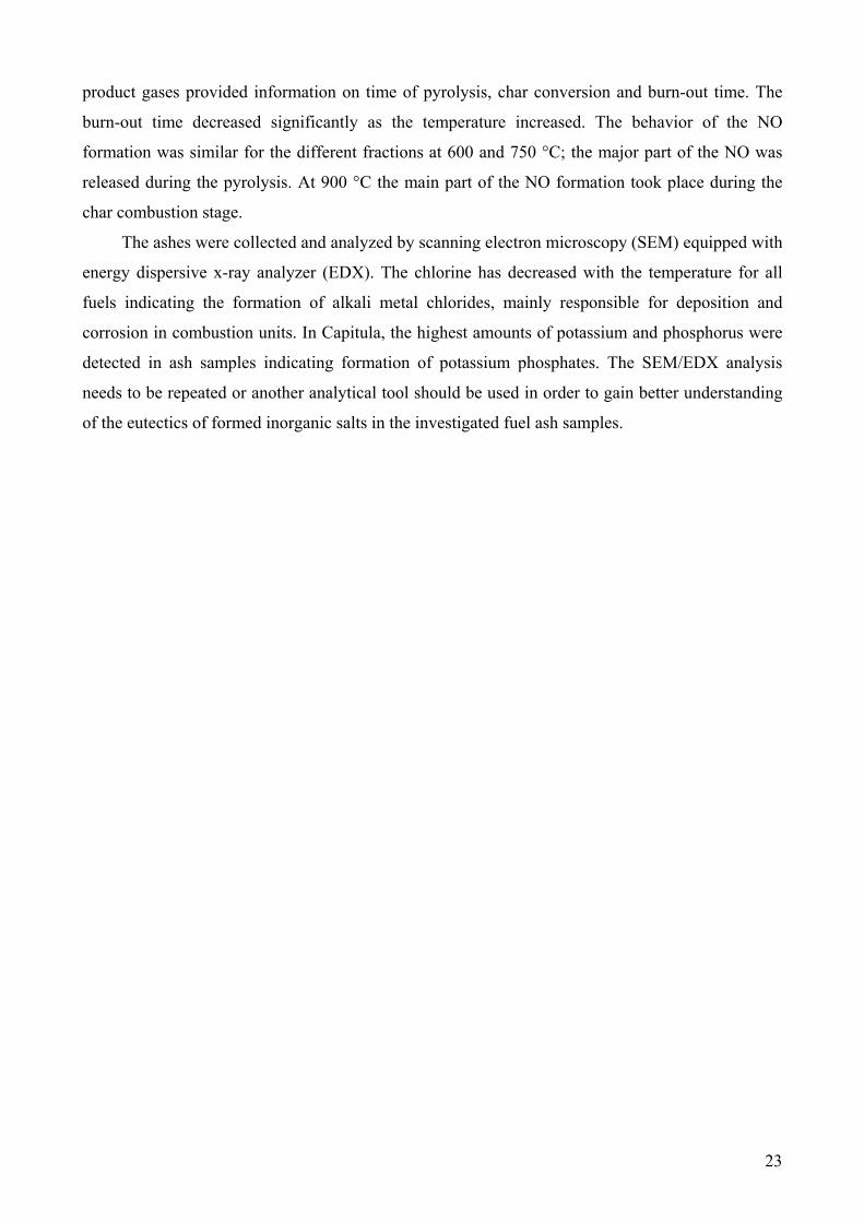
Only one spot was analyzed in ash sample for Leaves and is shown in Figure 21. The
composition of the single spot is almost similar to those analyzed in Stem, with the difference that
in the Leaves less potassium was detected in that particular spot.
Two spots were analyzed in ash particle from Capitula and is shown in Figure 22. The main
difference between the Stem spot analyses is a much higher potassium content in the analyzed spot.
0
5
10
15
20
25
30
35
40
45
Al Ca Fe K Mg Na P Si S Cl
wt-%
StemLeavesCapitula
Figure 18 Elemental composition from SEM/EDX of ash samples (550ºC).
20
0
5
10
15
20
25
30
35
40
45
50
55
60
65
Al Ca K Mg Na P Si S Cl
wt-%
StemLeavesCapitula
Figure 19 Elemental composition from SEM/EDX of ash samples (900ºC).
0
10
20
30
40
50
60
70
Al Ca K Mg Na P Si S Cl
wt-%
Stem spot1Stem spot2
Figure 20 SEM/EDX spot analysis results for particle in ash from Stem (900ºC).
21
0
10
20
30
40
50
60
70
80
Al Ca K Mg Na P Si S Cl
wt-%
Leaves spot1
Figure 21 SEM/EDX spot analysis for particle in ash from Leaves (900 ºC).
0
10
20
30
40
50
60
70
Al Ca K Mg Na P Si S Cl
wt-%
Capitula spot1Capitula spot2
Figure 22 SEM/EDX spopt analysis for particle in ash from Capitula (900 ºC).
5 CONCLUSIONS
Three fractions of Cynara were combusted in a laboratory scale fixed-bed reactor at three
different temperatures - 600, 750 and 900 °C - in an atmosphere of 10 % O and 90 % N . The O2 2 2,
SO , CO, CO and NO molar fractions of the product gases were measured. The analysis of the 2 2
22
product gases provided information on time of pyrolysis, char conversion and burn-out time. The
burn-out time decreased significantly as the temperature increased. The behavior of the NO
formation was similar for the different fractions at 600 and 750 °C; the major part of the NO was
released during the pyrolysis. At 900 °C the main part of the NO formation took place during the
char combustion stage.
The ashes were collected and analyzed by scanning electron microscopy (SEM) equipped with
energy dispersive x-ray analyzer (EDX). The chlorine has decreased with the temperature for all
fuels indicating the formation of alkali metal chlorides, mainly responsible for deposition and
corrosion in combustion units. In Capitula, the highest amounts of potassium and phosphorus were
detected in ash samples indicating formation of potassium phosphates. The SEM/EDX analysis
needs to be repeated or another analytical tool should be used in order to gain better understanding
of the eutectics of formed inorganic salts in the investigated fuel ash samples.
23
6 REFERENCES
1. Date of access (05-02-2009),
http://www.botanik.uni-karlsruhe.de/garten/fotos-
knoch/Cynara%20cardunculus%20Wilde%20Artischocke%201.jpg
2. Notes for course ‘Combustion and Harmful Emission Control’, [28244 E08], (2002), Institute
for Kemiteknik, Danish Technical University, Lyngby.
24