Course Syllabus for Math 287: Algebraic L-Theory

and Surgery

Course Description Let X be a finite complex. When does X has the homotopy type ofa smooth manifold? First, X must satisfy Poincare duality. Second, there should be avector bundle TX on X which plays the role of the tangent bundle. If the dimension ofX is divisible by 4, then the signature of the intersection form on the cohomology H∗(X)should be given as a certain characteristic class of TX (the Hirzebruch signature formula).Amazingly, if X is simply connected and has dimension 4k > 4, then these conditionsare sufficient to guarantee that X is homotopy equivalent to a smooth manifold. In thiscourse, we will study this theorem and some of its generalizations: to manifolds which arenot assumed to be smooth, to manifolds which are not assumed to be simply connected,and to manifolds whose dimension is not assumed to be divisible by four. In order toobtain a classification theorem in these settings, we will develop the subject of algebraicL-theory, which can be regarded as an elaborate generalization of the classical Witt groupsof quadratic forms.

Meeting Time MWF at 1.

Office Hours Thursdays 2-3, or by appointment.

Texts There is no textbook required for this class. Useful references include Ranicki’s “Alge-braic L-Theory and Topological Manifolds” and Wall’s text “Surgery on Compact Mani-folds.”

Course Website http://www.math.harvard.edu/∼lurie/287.html

Prerequisites Familiarity with the machinery of modern algebraic topology (simplicial sets,spectra, ...). The first part of the course (where we develop the subject of L-theory) willrequire a high tolerance for abstraction, while the second part (where we apply the theoryto classify manifolds) will be more concrete.

Topics likely to be covered • Construction of L-theory spectra.

• Witt groups of quadratic forms.

• Techniques of surgery in algebraic and geometric settings.

• Poincare duality spaces and Spivak normal fibrations.

• L-theory orientations and generalized signature formulas.

• Classification of high-dimensional manifolds, up to h-cobordism.

Grading Undergraduates or graduate students wishing to take this course for a grade shouldspeak with the instructor.

Introduction (Lecture 1)

February 2, 2011

In this course, we will be concerned with variations on the following:

Question 1. Let X be a CW complex. When does there exist a homotopy equivalence X ' M , where Mis a compact smooth manifold?

In other words, what is special about the homotopy type of a compact smooth manifold M? One specialfeature is obvious:

Fact 2. Compact manifolds satisfy Poincare duality.

Let us assume for simplicity that X is simply connected. If M is a compact smooth manifold homotopyequivalent to X, M is also simply connected and therefore orientable. A choice of orientation determinesa fundamental homology class [M ] ∈ Hn(M ; Z), where n denotes the dimension of M . If f : M → X is ahomotopy equivalence, then [X] = f∗[X] is an element of Hn(X; Z) with the following property: for everyinteger q, the operation of cap product with [X] induces an isomorphism

Hq(X; Z)→ Hn−q(X; Z).

This motivates the following definition:

Definition 3. Let X be a simply connected CW complex. We say that X is a simply connected Poincarecomplex of dimension n if there exists a homology class [X] ∈ Hn(X; Z) such that cap product with [X]induces isomorphisms

Hq(X; Z)→ Hn−q(X; Z)

for every integer q. In this case, we say that [X] is a fundamental class of X.

Example 4. Any compact smooth manifold of dimension n is a Poincare complex of dimension n.

Remark 5. Taking q = 0 in Definition 3 and using our assumption that X is connected, we obtain anisomorphism

Z ' H0(X; Z)→ Hn(X; Z)

given by 1 7→ [X]. It follows that Hn(X; Z) must be a free abelian group of rank 1, and [X] must be agenerator of Hn(X; Z). Consequently, the fundamental class of X is well-defined up to sign.

Remark 6. If X is a simply connected Poincare complex of dimension n, then we have

Hq(X; Z) ' Hn−q(X; Z) ' 0

for q > n. In particular, n is uniquely determined by X: it is the largest degree of a nonvanishing homologygroup of X.

Remark 7. Using the fact that Hm(X; Z) vanishes for m > n and that it is free when m = n, one can showthat X is homotopy equivalent to a CW complex whose cells have dimension ≤ n. However, we will notneed this fact and we will not require that X itself have this property.

1

We can now give a partial answer to Question 1: if X is to be homotopy equivalent to a compact smoothmanifold, then X must be a Poincare complex. We can therefore refine Question 1 (in the simply connectedcase) as follows:

Question 8. Let X be a simply connected Poincare complex of dimension n. When does there exist ahomotopy equivalence X 'M , where M is a smooth manifold of dimension n?

To address Question 8, we make another observation: if M is a smooth manifold of dimension n, thenM has a tangent bundle TM , which is a real vector bundle of rank n over M . Moreover, the tangent bundleof M is closely connected with our discussion of Poincare duality.

We begin by considering the normal bundle of M . Choose an embedding i : M → Rk for some largeinteger k. Let NM denote the normal bundle to this embedding. By choosing a tubular neighborhood of Min Rk, we can identify NM with an open subset of Rk. The Thom space T (NM ) is given by the one-pointcompactification of NM , given by NM ∪ ∗. We have a Thom-Pontryagin collapse map

c : Sk = Rk ∪∞ → T (NM ),

given by c(v) =

v if v ∈ N∗ otherwise.

which determines an element [c] ∈ πk(T (NM ),∞). Since M is simply

connected, the normal bundle N is oriented. Choosing an orientation, we obtain a Thom isomorphismHk(T (NM ), ∗; Z) ' Hn(M ; Z). Composing with the Hurewicz map, we obtain a homomorphism

πk(T (NM ), ∗)→ Hk(T (NM ), ∗; Z) ' Hn(M ; Z).

The image of [c] under this composite map is a fundamental homology class [M ]. (with respect to theorientation determined by the choice of orientation on NM ).

The vector bundle NM is not unique: it depends on a choice of embedding M → Rk. However, thespectrum Σ∞−kT (NM ) is uniquely determined. We have a canonical exact sequence of vector bundles

TM → TRn |M → NM .

Choosing a splitting of this exact sequence, we obtain a direct sum decomposition NM ⊕ TM ' Rk, whereRk denotes the trivial vector bundle of rank k. It follows that the spectrum Σ∞−kT (NM ) can be identifiedwith the Thom spectrum M−TM of the virtual vector bundle −TM on M . The element [c] ∈ πk(T (NM ),∞)determines an element ηM ∈ π0M−TM , which is independent of the choice of embedding i.

We can summarize the above discussion as follows:

Fact 9. Let M be a simply connected smooth manifold of dimension n. Then there exists a vector bundleζ on M of dimension n (namely, the tangent bundle TM ) and a class ηM ∈ π0M−ζ such that the image ofηM under the composite map

π0(M−ζ)→ H0(M−ζ ; Z) ' Hn(M ; Z)

is a fundamental class of M . Here the second map is the Thom isomorphism (determined by a choice oforientation of ζ).

This gives us another necessary condition that a simply connected CW complex X must satisfy if X isto be homotopy equivalent to a manifold of dimension n: there must exist a vector bundle ζ on X and ahomotopy class ηX ∈ π0X−ζ whose image [X] ∈ Hn(X; Z) exhibits X as a Poincare complex of dimensionn. We may therefore refine our question yet again:

Question 10. Let X be a simply connected Poincare complex of dimension n. Suppose we are given avector bundle ζ of dimension n on X and a homotopy class ηX ∈ π0X

−ζ whose image in Hn(X; Z) is afundamental homology class for X. Does there exist a smooth manifold M of dimension n and a homotopyequivalence f : M → X such that f∗ζ is (stably) isomorphic to TM and f∗ηX = ηM ∈ π0M−TM ?

2

We now give the answer to Question 10 in the simplest case. Assume that X is a simply connectedPoincare complex of dimension n = 4k. In this case, we have a symmetric bilinear form

〈, 〉 : H2k(X;R)×H2k(X;R)→ H4k(X;R)[X]→ R

and Poincare duality ensures that this form is nondegenerate. We may therefore choose an orthogonal basis(x1, . . . , xa, y1, . . . , yb) for H2k(X;R) satisfying 〈xi, xi〉 = 1 and 〈yi, yi〉 = −1. The difference a − b is calledthe signature of X, and will be denoted by σX . Note that the sign of σX depends on a choice of fundamentalclass for X.

If M is a compact smooth manifold of dimension n = 4k, then the signature of M is given by theHirzebruch signature formula. Namely, there is a formula

σM = L(p1(TM ), p2(TM ), . . . , pk(TM ))[M ].

Here L(p1(TM ), p2(TM ), . . . , pk(TM )) denotes some polynomial in the Pontryagin classes pi(TM ) (note thatthe right hand side of this formula also depends up to sign on our choice of orientation of M). For example,

when n = 4 we have σM = p1(TM )3 [M ], and when n = 8 we have

σM =7p2(TM )− p1(TM )2

45[M ].

Remark 11. If we choose a connection on the manifold M , then we can use Chern-Weil theory to obtainexplicit differential forms representing the Pontryagin classes of the tangent bundle TM . Consequently, thesignature of M can be computed by integrating over M an explicitly given n-form on M . We can thereforeregard the Hirzebruch signature formula as saying that there is a purely local formula for the signature, whichis defined a priori as a global invariant of M .

Remark 12. Here is a very rough heuristic justification for why there should exist a Hirzebruch signatureformula. If X is a Poincare complex of dimension 4k, then the signature σX is defined because we candefine an intersection form using Poincare duality. If X is a manifold, the Poincare duality is satisfied for a“local” reason, so we might expect to obtain a “local” formula for σX . Later in this course, we will provethe Hirzebruch signature formula by making this heuristic more precise.

This gives us one further condition that a triple, (X, ζ, νX ∈ π0X−ζ) must satisfy to obtain an affirmativeanswer to Question 10. Namely, we must have

σX = L(p1(ζ), p2(ζ), . . . , pk(ζ))[X].

Simply-connected surgery provides a converse in high dimensions:

Theorem 13 (Browder, Novikov?). Let X be a simply connected Poincare complex of dimension 4k >4, let ζ be a vector bundle (of rank 4k) on X, and let ηX ∈ π0X

−ζ be such that the image of ηX inH4k(X; Z) is a fundamental class. Then Question 10 has an affirmative answer if and only if σX =L(p1(ζ), p2(ζ), . . . , pk(ζ))[X]: that is, if and only if X satisfies the Hirzebruch signature formula.

Theorem 13 is a prototype for the type of result we would like to obtain in this class. We will pursue anumber of variations:

(a) We can contemplate Question 1 for Poincare complexes X which are not assumed to be simply con-nected.

(b) Question 1 concerns the existence of a manifold M in the homotopy type of X. If the answer isaffirmative, one can further ask if M is unique.

3

Let us briefly describe how problem (b) can be attacked. Suppose that we are given a Poincare complexX and a pair of homotopy equivalences f : X →M , g : X →M ′, where M and M ′ are compact manifolds ofdimension n. We can then consider the “double mapping cylinder” Y = M

∐X×0(X × [0, 1])

∐X×1M

′.

The pair (Y,M qM ′) satisfies a relative version of Poincare duality. This suggests that we might look foran (n + 1)-manifold B with boundary M qM ′ and a homotopy equivalence (B,M qM ′) → (Y,M qM ′)which restricts to the identity map on M and M ′. If we can solve this problem, then B is an h-cobordismfrom M to M ′: that is, a bordism from M to M ′ such that the inclusions M → B ← M ′ are homotopyequivalences. If n ≥ 5 and M is simply connected, then the h-cobordism theorem guarantees the existenceof a diffeomorphism B 'M × [0, 1], which in particular gives a diffeomorphism M 'M ′.

In summary, the problem of deciding whether M is unique can be regarded as another of roughly thesame type as Question 1. This motivates considering two more types of variations of Question 1:

(c) Rather than considering the absolute case of a Poincare complex X, we should consider the problemof proving that a pair of spaces (X, ∂ X) is homotopy equivalent to a manifold with boundary.

(d) We should not restrict our attention to the case of a fixed dimension n: a lot of information about theclassification of manifolds of dimension n can be obtained by thinking about manifolds of dimension> n. In particular, we should not restrict our attention to the case where n is a multiple of four.(However, we will retain the assumption that n > 4: this is the domain of high-dimensional topologywhere techniques of surgery work well).

If M is not simply connected, then an h-cobordism from M to M ′ does not generally guarantee that Mand M ′ are diffeomorphic: one encounters an algebraic obstruction called the Whitehead torsion. This isan interesting story, but not one we will discuss in this class: we will be content to give the classification ofmanifolds in a homotopy type up to h-cobordism.

In fact, we will do more. Suppose that M and M ′ are as above, and that Y has the homotopy type of anh-cobordism B from M to M ′. We might then ask a higher-order uniqueness question: to what extent is thebordism B uniquely determined? To ask these questions in an organized way, it is convenient to introducethe structure space S(X) of a Poincare complex X. This is a space whose connected components are givenby manifolds M with a homotopy equivalence M → X, up to h-cobordism. Question 1 is the question ofwhether or not S(X) is nonempty, and the uniqueness problem amounts to the question of whether or notS(X) is connected. Better still, we might try to discuss the entire homotopy type of S(X).

(e) We can ask an analogue of Question 1 for manifolds equipped with various structure. Suppose, forexample, that we wanted to find a spin manifold in the homotopy type of the Poincare complex X.The collection of h-cobordism classes of such manifolds can be described as connected components of aslightly different structure space SSpin(X). By forgetting spin structures, we obtain a map of structurespaces θ : SSpin(X) → S(X). Giving a spin structure on a manifold M is equivalent to giving a spinstructure on its tangent bundle TM : that is, to reducing the structure group of M from the orthogonalgroup Ø(n) to the spin group Spin(N). Consequently, the homotopy fibers of the map θ are easy todescribe. Consequently, the problem of determining the homotopy type of SSpin(X) can be reduced tothe problem of determining the homotopy type of S(X).

What we have denoted by S(X) should really be denoted SSm(X), the smooth structure space, becausein the above discussion we required all manifolds to be smooth. We can also define a topologicalstructure space STop(X) by considering topological manifolds with a homotopy equivalence to X.By forgetting smooth structures, we obtain a map of structures spaces SSm(X) → STop(X). Therelationship between SSm(X) and STop(X) is similar to the relationship between SSpin(X) and SSm(X):according to smoothing theory, for topological manifolds M of dimension > 4, giving a smooth structureon M is equivalent giving a vector bundle structure on the topological tangent bundle TM . In otherwords, to classify smooth manifolds in the homotopy type of X we can proceed by first classifying thetopological manifolds in the homotopy type of X and then studying the problem of smoothing them,

4

where the second step reduces to a purely homotopy-theoretic problem. Put another way, there is agood homotopy-theoretic understanding of the homotopy fibers of the map SSm(X)→ STop(X).

However, there is a much more compelling reason to work with topological manifolds rather thansmooth manifolds: the topological versions of these questions often have nicer answers. For example,there is only one topological manifold in the homotopy type of the n-sphere Sn (by the generalizedPoincare conjecture), but this topological manifold admits many different smooth structures (exoticspheres). The ultimate algebraic description of structure spaces which we obtain will be cleanest inthe topological category. For example, SSm(X) is just a space, but we will later see that STop(X) is aninfinite loop space (if nonempty). A concrete consequence of this is that if we fix a topological manifoldM , then the collection of h-cobordism classes of manifolds in with a homotopy equivalence to M hasthe structure of an abelian group.

Our ultimate goal in this course is to obtain a purely homotopy theoretic description of the structurespace S(X) of a Poincare complex X. Though we are not yet ready to formulate this description precisely,let us assert that it has the same basic form as the statement of Theorem 13. Namely, we will associateto X a certain invariant σ, called the visible symmetric signature of X. We will then show that finding amanifold in the homotopy type of X amounts to verifying a “local formula” for this invariant, generalizingthe Hirzebruch signature formula (see Remark 11). The fine print is that this invariant is not an integer,but something more sophisticated. Explaining exactly what that “something” is will require us to developthe apparatus of algebraic L-theory. That is our objective for the first half of this course. In the second half,we will return to the theory of manifolds, using the algebraic apparatus to prove a very general version ofTheorem 13.

5

Categorical Background (Lecture 2)

February 2, 2011

In the last lecture, we stated the main theorem of simply-connected surgery (at least for manifolds ofdimension 4m), which highlights the importance of the signature σX as an invariant of an (oriented) Poincarecomplex. Let us begin with a few remarks about how this invariant is defined.

Let V be a finite dimensional vector space over the real numbers and let q : V → R be a nondegeneratequadratic form on V , with associated bilinear form (, ) : V × V → R. We can always choose an orthogonalbasis x1, . . . , xa, y1, . . . , yb for V satisfying

(xi, xi) = 1 (yi, yi) = −1.

The sum a + b is the dimension of the vector space V , and the difference a − b is called the signature of q,and denoted σ(q).

Theorem 1 (Sylvester). Let V be a finite dimensional vector space over R equipped with a nondegeneratequadratic form q : V → R. Then the signature σ(q) is well-defined: that is, it does not depend on thechoice of orthogonal basis for V . Moreover, if V ′ is another finite dimensional vector space over R with aquadratic form q′ : V ′ → R, then there exists an isometry (V, q) ' (V ′, q′) if and only if dimV = dimV ′ andσ(q) = σ(q′).

The notion of a vector space V with a quadratic form makes sense over an arbitrary field k. We haveemphasized the case k = R for two reasons: first, the classification of quadratic forms over R is particularlysimple (because of Theorem 1). Second, information about the intersection form on the middle cohomologyH2m(X;R) of a simply connected Poincare complex of dimension 4m plays an important role in determiningwhether or not X is homotopy equivalent to a manifold. However, quadratic forms over other fields are alsoof geometric interest. For example, if X is a simply connected Poincare complex of dimension 4m + 2 > 4,then the problem of finding a manifold in the homotopy type of X turns out to depend on more subtleproperties of quadratic forms over the field F2. We would ultimately like to treat manifolds of all dimensionsin a uniform way, which will require us to somehow interpolate between the fields k = R and k = F2. Wecan do this by considering quadratic forms over the integers, or over more general rings.

The theory of quadratic forms over an arbitrary ring R can be very complicated. For example, theclassification of quadratic forms over the field Q of rational numbers is a nontrivial achievement in numbertheory (the Hasse-Minkowski theorem). In general, we cannot detect whether two quadratic forms areisomorphic by means of simple integer invariants, as in Theorem 1. However, there are more elaboratetheories that are designed to generalize the dimension and signature to other contexts:

1

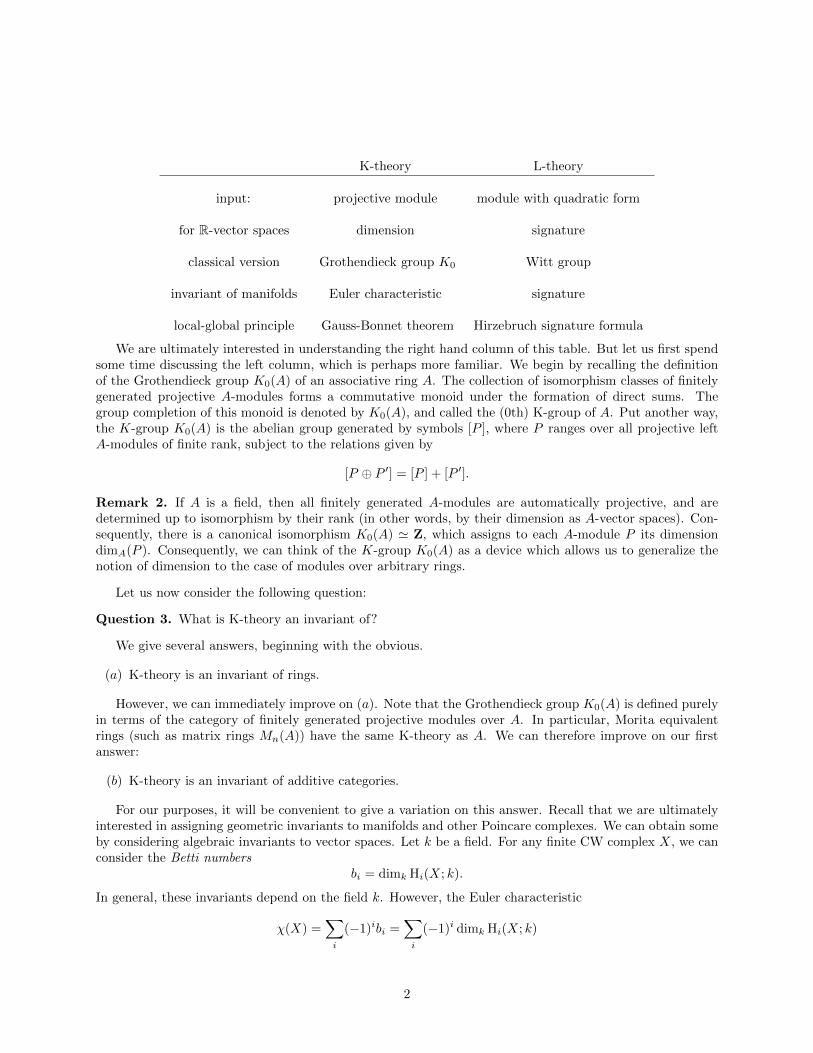
K-theory L-theory

input: projective module module with quadratic form

for R-vector spaces dimension signature

classical version Grothendieck group K0 Witt group

invariant of manifolds Euler characteristic signature

local-global principle Gauss-Bonnet theorem Hirzebruch signature formula

We are ultimately interested in understanding the right hand column of this table. But let us first spendsome time discussing the left column, which is perhaps more familiar. We begin by recalling the definitionof the Grothendieck group K0(A) of an associative ring A. The collection of isomorphism classes of finitelygenerated projective A-modules forms a commutative monoid under the formation of direct sums. Thegroup completion of this monoid is denoted by K0(A), and called the (0th) K-group of A. Put another way,the K-group K0(A) is the abelian group generated by symbols [P ], where P ranges over all projective leftA-modules of finite rank, subject to the relations given by

[P ⊕ P ′] = [P ] + [P ′].

Remark 2. If A is a field, then all finitely generated A-modules are automatically projective, and aredetermined up to isomorphism by their rank (in other words, by their dimension as A-vector spaces). Con-sequently, there is a canonical isomorphism K0(A) ' Z, which assigns to each A-module P its dimensiondimA(P ). Consequently, we can think of the K-group K0(A) as a device which allows us to generalize thenotion of dimension to the case of modules over arbitrary rings.

Let us now consider the following question:

Question 3. What is K-theory an invariant of?

We give several answers, beginning with the obvious.

(a) K-theory is an invariant of rings.

However, we can immediately improve on (a). Note that the Grothendieck group K0(A) is defined purelyin terms of the category of finitely generated projective modules over A. In particular, Morita equivalentrings (such as matrix rings Mn(A)) have the same K-theory as A. We can therefore improve on our firstanswer:

(b) K-theory is an invariant of additive categories.

For our purposes, it will be convenient to give a variation on this answer. Recall that we are ultimatelyinterested in assigning geometric invariants to manifolds and other Poincare complexes. We can obtain someby considering algebraic invariants to vector spaces. Let k be a field. For any finite CW complex X, we canconsider the Betti numbers

bi = dimk Hi(X; k).

In general, these invariants depend on the field k. However, the Euler characteristic

χ(X) =∑i

(−1)ibi =∑i

(−1)i dimk Hi(X; k)

2

does not depend on k. This invariant χ(X) is not generally not the dimension of a vector space (for example,it can be negative). Instead, we should think of it as an invariant of a chain complex of vector spaces: thesingular chain complex C∗(X; k).

More generally, we would like to say that for any ring A, the chain complex C∗(X;A) determines a classin the Grothendieck group K0(A). (Of course, we know what this class should be: namely, χ(X)[A] ∈ K0(A).Ignore this for the moment.) We generally cannot define this class to be the alternating sum∑

i

(−1)i[Hi(X;A)],

because the individual A-modules Hi(X;A) need not be projective.To show that C∗(X;A) determines a well-defined class in the group K0(A), it is convenient to describe

K0(A) in a different way. Rather than representing K-theory classes by projective modules over A, we takeas representatives chain complexes of modules over A. Of course, we do not want to allow arbitrary chaincomplexes. In order to obtain reasonable invariants, we should restrict our attention to chain complexes whichare perfect: that is, which are quasi-isomorphic to bounded chain complexes of finite projective modules. IfX is a finite CW complex, then the singular chain complex C∗(X;A) is always perfect: for example, it isquasi-isomorphic to the chain complex which computes the cellular homology of X.

Let Perf denote the category whose objects are bounded chain complexes of finite projective modules.For every perfect complex M•, we can find a quasi-isomorphism P• → M•, where P• ∈ Perf . The chaincomplex P• need not be unique. However, it is unique up to chain homotopy equivalence. We can obtain astronger uniqueness result by passing to the homotopy category. Let hPerf be the category with the sameobjects as Perf , but whose morphisms are given by chain homotopy classes of chain maps. The categoryhPerf is called the perfect derived category of A. Every perfect complex of A-modules determines an objectof hPerf , which is well-defined up to isomorphism. Moreover, hPerf is an example of a triangulated category:that is, there is a notion of distinguished triangle

P ′• → P• → P ′′• → P ′•[1]

in hPerf . Let K ′0(A) denote the abelian group generated by symbols [P•], where P• is an object of hPerf ,with relations [P•] = [P ′•] + [P ′′• ] for every distinguished triangle

P ′• → P• → P ′′• → P ′•[1].

Every finitely generated projective A-module can be regarded as a perfect complex which is concentrated indegree zero, and this construction determines a map of abelian groups K0(A)→ K ′0(A). One can show thatthis map is an isomorphism. In other words, one can define the Grothendieck group using (perfect) chaincomplexes of modules, rather than individual modules. With this definition, it is easy to see that C∗(X;A)determines a well-defined K-theory class, for every finite CW complex X. This suggests a different answerto Question 3:

(c) K-theory is an invariant of triangulated categories.

For purposes of this course, answer (c) is a little bit misleading. The passage from the category Perfto its homotopy category hPerf has upsides and downsides. It has the virtue of allowing us to treat quasi-isomorphic chain complexes as if they are actually isomorphic. Unfortunately, it also loses a lot of information,because it has the effect of identifying chain homotopic morphisms without remembering any informationabout the chain homotopy. For our purposes, we will need to work with an intermediate object Dperf(A),which will allow us to treat quasi-isomorphisms between chain complexes as if they were isomorphisms whileretaining information about chain homotopies. The fine print is that unlike Perf and hPerf , Dperf(A) isnot a category: rather it is a more general object called an ∞-category.

We are now ready to give our final answer to Question 3:

(d) K-theory is an invariant of stable ∞-categories.

3

Our goal in this lecture and the next is to explain the meaning of this statement. To do so will requirea long digression.

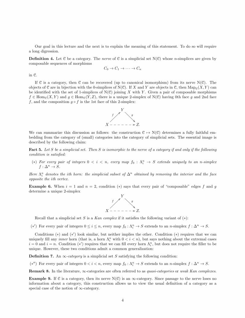
Definition 4. Let C be a category. The nerve of C is a simplicial set N(C) whose n-simplices are given bycomposable sequences of morphisms

C0 → C1 → · · · → Cn

in C.

If C is a category, then C can be recovered (up to canonical isomorphism) from its nerve N(C). Theobjects of C are in bijection with the 0-simplices of N(C). If X and Y are objects in C, then MapC(X,Y ) canbe identified with the set of 1-simplices of N(C) joining X with Y . Given a pair of composable morphismsf ∈ HomC(X,Y ) and g ∈ HomC(Y,Z), there is a unique 2-simplex of N(C) having 0th face g and 2nd facef , and the composition g f is the 1st face of this 2-simplex:

Yg

X

f>>

// Z.

We can summarize this discussion as follows: the construction C 7→ N(C) determines a fully faithful em-bedding from the category of (small) categories into the category of simplicial sets. The essential image isdescribed by the following claim:

Fact 5. Let S be a simplicial set. Then S is isomorphic to the nerve of a category if and only if the followingcondition is satisfied:

(∗) For every pair of integers 0 < i < n, every map f0 : Λni → S extends uniquely to an n-simplex

f : ∆n → S.

Here Λni denotes the ith horn: the simplicial subset of ∆n obtained by removing the interior and the face

opposite the ith vertex.

Example 6. When i = 1 and n = 2, condition (∗) says that every pair of “composable” edges f and gdetermine a unique 2-simplex

Yg

X

f>>

// Z.

Recall that a simplicial set S is a Kan complex if it satisfies the following variant of (∗):

(∗′) For every pair of integers 0 ≤ i ≤ n, every map f0 : Λni → S extends to an n-simplex f : ∆n → S.

Conditions (∗) and (∗′) look similar, but neither implies the other. Condition (∗) requires that we canuniquely fill any inner horn (that is, a horn Λn

i with 0 < i < n), but says nothing about the extremal casesi = 0 and i = n. Condition (∗′) requires that we can fill every horn Λn

i , but does not require the filler to beunique. However, these two conditions admit a common generalization:

Definition 7. An ∞-category is a simplicial set S satisfying the following condition:

(∗′′) For every pair of integers 0 < i < n, every map f0 : Λni → S extends to an n-simplex f : ∆n → S.

Remark 8. In the literature, ∞-categories are often referred to as quasi-categories or weak Kan complexes.

Example 9. If C is a category, then its nerve N(C) is an ∞-category. Since passage to the nerve loses noinformation about a category, this construction allows us to view the usual definition of a category as aspecial case of the notion of ∞-category.

4

Example 10. Any Kan complex is an∞-category. In particular, if X is a topological space, then the singularcomplex Sing(X) (whose n-simplices are given by continuous maps from a topological n-simplex into X) isan ∞-category. Since the singular complex Sing(X) determines X up to weak homotopy equivalence, notmuch information is lost by the construction X 7→ Sing(X). Consequently, for many purposes, we can thinkof ∞-categories as a generalization of topological spaces.

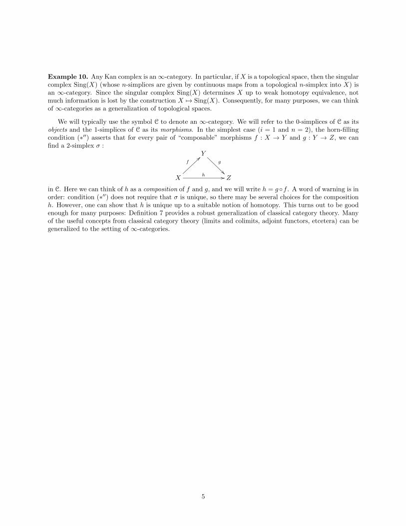
We will typically use the symbol C to denote an ∞-category. We will refer to the 0-simplices of C as itsobjects and the 1-simplices of C as its morphisms. In the simplest case (i = 1 and n = 2), the horn-fillingcondition (∗′′) asserts that for every pair of “composable” morphisms f : X → Y and g : Y → Z, we canfind a 2-simplex σ :

Yg

X

f>>

h // Z

in C. Here we can think of h as a composition of f and g, and we will write h = g f . A word of warning is inorder: condition (∗′′) does not require that σ is unique, so there may be several choices for the compositionh. However, one can show that h is unique up to a suitable notion of homotopy. This turns out to be goodenough for many purposes: Definition 7 provides a robust generalization of classical category theory. Manyof the useful concepts from classical category theory (limits and colimits, adjoint functors, etcetera) can begeneralized to the setting of ∞-categories.

5

Stable ∞-Categories (Lecture 3)

February 2, 2011

In the last lecture, we introduced the definition of an∞-category as a generalization of the usual notion ofcategory. This definition is one way of formalizing the notion of a higher category in which all k-morphismsare invertible for k > 1. Many other approaches are possible. The following is probably more intuitive:

Definition 1. A topological category is a category C together with a topology on the set HomC(X,Y ) forevery pair of objects X and Y , such that the composition maps HomC(X,Y )×HomC(Y,Z)→ HomC(X,Z)are continuous. (In other words, a category which is enriched over the category of topological spaces.) If Cis a topological category containing a pair of objects X and Y , we will denote HomC(X,Y ) by MapC(X,Y )when we wish to emphasize that we are thinking of it as a topological space.

Remark 2. To accommodate certain examples, it is convenient to modify Definition 1 by working with com-pactly generated topological spaces rather than topological spaces. That is, we require that each MapC(X,Y )be compactly generated, and require that composition is given by continuous maps

MapC(X,Y )×MapC(Y, Z)→ MapC(X,Z)

where the product is taken in the category of compactly generated topological spaces. This is a technicalpoint which may be safely ignored.

The theory of ∞-categories is closely related to the theory of topological categories.

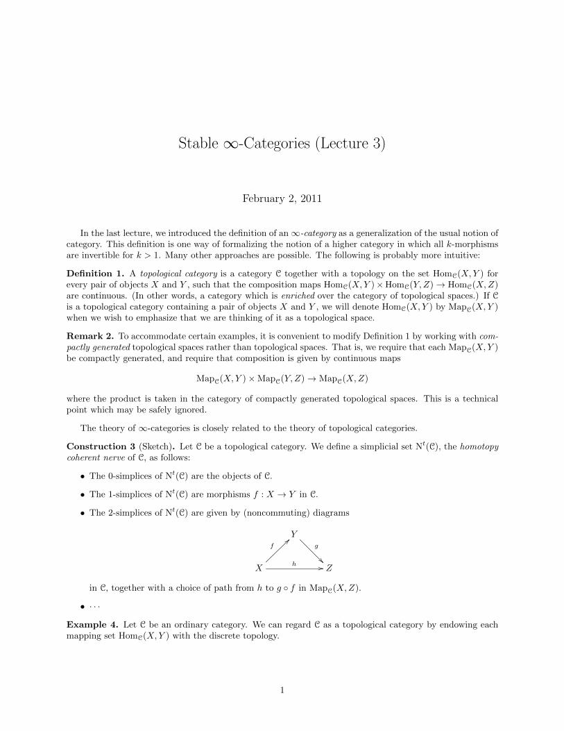
Construction 3 (Sketch). Let C be a topological category. We define a simplicial set Nt(C), the homotopycoherent nerve of C, as follows:

• The 0-simplices of Nt(C) are the objects of C.

• The 1-simplices of Nt(C) are morphisms f : X → Y in C.

• The 2-simplices of Nt(C) are given by (noncommuting) diagrams

Yg

X

f>>

h // Z

in C, together with a choice of path from h to g f in MapC(X,Z).

• · · ·

Example 4. Let C be an ordinary category. We can regard C as a topological category by endowing eachmapping set HomC(X,Y ) with the discrete topology.

1

It turns out that for any topological category C, the homotopy coherent nerve Nt(C) is an ∞-category.Moreover, there is a sort of converse: every∞-category is equivalent to Nt(C) for some topological category C,and the topological category C is essentially unique (up to a suitable notion of weak homotopy equivalence).In other words, the construction C 7→ Nt(C) determines an equivalence between the theory of topologicalcategories and the theory of ∞-categories. From this point forward, we will work at an informal level andfreely mix these two notions. For example, if S is an ∞-category containing a pair of 0-simplices x and y,we will use MapS(x, y) to denote a mapping space between x and y, when viewed as objects of a topologicalcategory whose homotopy coherent nerve is equivalent to S.

Remark 5. To any topological category C (and therefore to any ∞-category) we can associate an ordi-nary category hC, called the homotopy category of C. It has the same objects, with morphisms given byHomhC(X,Y ) = π0 MapC(X,Y ).

Example 6. The collection of finite CW complexes forms a topological category: for any pair of finite CWcomplexes X and Y , we can endow the set of continuous maps Hom(X,Y ) with the compact-open topology.If we use the convention of Remark 2, then this generalizes to arbitrary CW complexes. We will denotethe homotopy coherent nerve of this (larger) topological category by S, and refer to it as the ∞-category ofspaces.

Here is an example of greater interest to us:

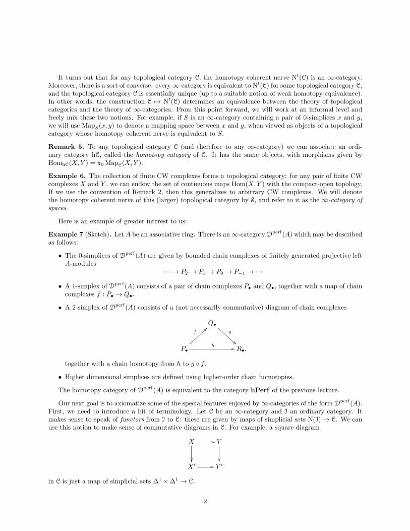
Example 7 (Sketch). Let A be an associative ring. There is an∞-category Dperf(A) which may be describedas follows:

• The 0-simplices of Dperf(A) are given by bounded chain complexes of finitely generated projective leftA-modules

· · · → P2 → P1 → P0 → P−1 → · · ·

• A 1-simplex of Dperf(A) consists of a pair of chain complexes P• and Q•, together with a map of chaincomplexes f : P• → Q•.

• A 2-simplex of Dperf(A) consists of a (not necessarily commutative) diagram of chain complexes

Q•g

!!P•

f>>

h // R•,

together with a chain homotopy from h to g f .

• Higher dimensional simplices are defined using higher-order chain homotopies.

The homotopy category of Dperf(A) is equivalent to the category hPerf of the previous lecture.

Our next goal is to axiomatize some of the special features enjoyed by∞-categories of the form Dperf(A).First, we need to introduce a bit of terminology. Let C be an ∞-category and I an ordinary category. Itmakes sense to speak of functors from I to C: these are given by maps of simplicial sets N(I)→ C. We canuse this notion to make sense of commutative diagrams in C. For example, a square diagram

X //

Y

X ′ // Y ′

in C is just a map of simplicial sets ∆1 ×∆1 → C.

2

Definition 8. Let C be an ∞-category. We will say that an object 0 ∈ C is a zero object if, for every objectX ∈ C, the mapping spaces

MapC(0, X) MapC(X, 0)

are contractible. We will say that C is pointed if it admits a zero object.

If C is a pointed ∞-category, then for any pair of objects X and Y there is a zero map from X to Y ,given by the composition

X → 0→ Y

where 0 is a zero object of C. This map is well-defined up to a contractible space of choices.

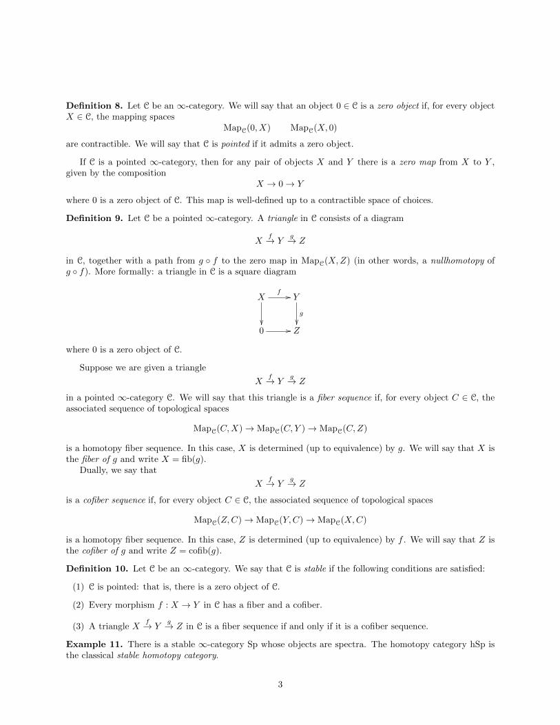
Definition 9. Let C be a pointed ∞-category. A triangle in C consists of a diagram

Xf→ Y

g→ Z

in C, together with a path from g f to the zero map in MapC(X,Z) (in other words, a nullhomotopy ofg f). More formally: a triangle in C is a square diagram

Xf //

Y

g

0 // Z

where 0 is a zero object of C.

Suppose we are given a triangle

Xf→ Y

g→ Z

in a pointed ∞-category C. We will say that this triangle is a fiber sequence if, for every object C ∈ C, theassociated sequence of topological spaces

MapC(C,X)→ MapC(C, Y )→ MapC(C,Z)

is a homotopy fiber sequence. In this case, X is determined (up to equivalence) by g. We will say that X isthe fiber of g and write X = fib(g).

Dually, we say that

Xf→ Y

g→ Z

is a cofiber sequence if, for every object C ∈ C, the associated sequence of topological spaces

MapC(Z,C)→ MapC(Y,C)→ MapC(X,C)

is a homotopy fiber sequence. In this case, Z is determined (up to equivalence) by f . We will say that Z isthe cofiber of g and write Z = cofib(g).

Definition 10. Let C be an ∞-category. We say that C is stable if the following conditions are satisfied:

(1) C is pointed: that is, there is a zero object of C.

(2) Every morphism f : X → Y in C has a fiber and a cofiber.

(3) A triangle Xf→ Y

g→ Z in C is a fiber sequence if and only if it is a cofiber sequence.

Example 11. There is a stable ∞-category Sp whose objects are spectra. The homotopy category hSp isthe classical stable homotopy category.

3

Example 12. The ∞-category Dperf(A) considered above is stable.

Let C be a stable ∞-category. We define an abelian group K0(C) as follows: K0(C) is obtained from thefree abelian group generated by symbols [X], where X is an object of C, subject to the following relation: ifthere is a fiber sequence

X → Y → Z,

then [Y ] = [X] + [Z].

Remark 13. Let C be a stable ∞-category. One can show that the homotopy category of C is triangulated.Moreover, theK-groupK0(C) depends only on the homotopy category of C, viewed as a triangulated category.However, when discussing more sophisticated invariants of C (like higher K-groups or L-groups) it is betternot to pass to the homotopy category.

Example 14. If A is a ring, then the K-group K0(Dperf(A)) is canonically isomorphic to the group K0(A)defined in the last lecture. In particular, if A is a field, then there is a canonical isomorphism K0(Dperf(A)) 'Z. If P• is an object of Dperf(A), then [P•] ∈ K0(Dperf(A)) ' Z can be identified with the Euler characteristic∑

i

(−1)i dimA Hi(P•)

of the chain complex P•.

In general, if we are given an object X of a stable ∞-category C, then we can view the class [X] ∈ K0(C)as a kind of “generalized Euler characteristic” of X. It is in general not an integer, but an element ofthe abelian group K0(C) which depends on C. We can think of the construction C 7→ K0(C) as a kind ofcategorificatied Euler characteristic:

Input Invariant

vector space V dimension dim(V ) ∈ Z

complex of vector spaces Euler characteristic χ ∈ Z

stable ∞-category C abelian group K0(C)

object of a stable ∞-category C K-theory class [X] ∈ K0(C)

However, these are not the invariants we really want to study in this class. Recall that if V is a finitedimensional vector space over R with a nondegenerate quadratic form q, then V is determined (up toisometry) by two invariants: the dimension of V and the signature of V . It is the latter that we would reallylike to generalize. Let us briefly indicate the form that this generalization will take:

Input Invariant

nondegenerate quadratic space (V, q) over R signature σ(V, q) ∈ Z

Poincare chain complex (V∗, q) over R signature σ of middle homology

stable ∞-category C with quadratic functor Q L-group L0(C, Q)

Object X ∈ C satisfying Poincare duality [X] ∈ L0(C, Q)

We will start making sense of some of these words in the next lecture.

4

Quadratic Functors (Lecture 4)

February 2, 2011

In this lecture, we will introduce the notion of a quadratic functor Q on a stable∞-category C, and definethe L-group L0(C, Q). We begin with a short review of the classical theory of quadratic forms.

Definition 1. Let M and A be abelian groups. An A-valued bilinear form on M is a map

b : M ×M → A

such that, for each x ∈ M , the maps y 7→ b(x, y) and y 7→ b(y, x) are abelian group homomorphisms fromM into A. We will say that b is symmetric if b(x, y) = b(y, x).

An inhomogeneous A-valued quadratic form on M is a map q : M → A such that q(0) = 0 and thefunction b(x, y) = q(x + y) − q(x) − q(y) is a bilinear form. We will say that q is a quadratic form if, inaddition, we have q(nx) = n2q(x) for every integer n and every x ∈M .

The theory of quadratic forms and bilinear forms are closely connected. If q is an inhomogeneous quadraticform on an abelian group M , then the function b(x, y) = q(x+ y)− q(x)− q(y) is a symmetric bilinear form.If multiplication by 2 is invertible on A, we can almost recover q from the bilinear form b: namely, wehave q(x) = 1

2b(x, x) + l(x) for some group homomomorphism l : M → A. In particular, the constructionb 7→ 1

2b(x, x) determines a bijective correspondence between symmetric bilinear forms and quadratic forms(whenever multiplication by 2 is invertible on A).

Our next goal is to categorify some of these ideas: that is, to make sense of the algebraic structuresdescribed above when the notion of module is replaced by some sort of category (in our case, stable ∞-categories). Let us begin by drawing up a table of analogies:

Classical Story Categorified Story

abelian group stable ∞-category

Z ∞-category Sp of spectra

abelian group homomorphism exact functor

(symmetric) bilinear form (symmetric) bilinear functor

inhomogeneous quadratic form quadratic functor

We now introduce some of the relevant definitions.

Definition 2. Let F : C→ D be a functor between stable ∞-categories. We say that F is exact if it carrieszero objects to zero objects and fiber sequences to fiber sequences.

Let Sp denote the ∞-category of spectra.

1

Definition 3. Let C be a stable ∞-category. A bilinear functor on C is a functor

B : Cop×Cop → Sp

with the following property: for every object C ∈ C, the functors

D 7→ B(C,D) D 7→ B(D,C)

are exact functors from Cop to Sp.The collection of bilinear functors on C is evidently acted on by the symmetric group Σ2 on two letters

(by permuting the arguments). A symmetric bilinear functor is a homotopy fixed point for this action.

Let C be a stable ∞-category containing an object X. For every object Y , the sequence of mappingspaces MapC(Y,ΣnX)n≥0 constitutes a spectrum (that is, each is homotopy equivalent to the loop spaceon the next). We will denote this spectrum by MorC(Y,X). The construction Y 7→ MorC(Y,X) determinesan (exact) functor from Cop to Sp. We will say that a functor F : Cop → Sp is representable if it arises inthis way.

Suppose that B : Cop×Cop → Sp is a symmetric bilinear functor. We will say that B is representable if,for all X ∈ C, the functor Y 7→ B(X,Y ) is representable. In this case, we write B(X,Y ) = MorC(Y,DX)for some object DX in C, which is determined up to contractible ambiguity. The construction X 7→ DXdetermines a functor from C to Cop. For each X ∈ C, the identity map idDX determines point in thezeroth space of B(X,DX) ' B(DX,X), and therefore a morphism eX : X → D2X. We will say that B isnondegenerate if it is representable and the canonical map eX is an equivalence for every X ∈ C.

Example 4. Let C be the ∞-category of spectra, and let ∧ denote the smash product functor. The functorB(X,Y ) = MorSp(X ∧ Y, S) determines a symmetric bilinear functor on C. This symmetric bilinear functoris representable, and the corresponding functor D : C → C is Spanier-Whitehead duality. If we restrict ourattention to the full subcategory of C spanned by the finite spectra, then B becomes nondegenerate.

Definition 5. Let C be a stable ∞-category. We say that a functor Q : Cop → Sp is reduced if Q carrieszero objects to zero objects. In this case, Q carries also carries zero morphisms to zero morphisms.

Let Q : Cop → Sp be a reduced functor. If X,Y ∈ C, we obtain maps

Q(X)⊕Q(Y )→ Q(X ⊕ Y )→ Q(X)⊕Q(Y )

where the composition is given by applying Q to the matrix[idX 00 idY

]If Q is reduced, this map is the identity so that Q(X)⊕Q(Y ) is a summand of Q(X ⊕ Y ); that is, we havea direct sum decomposition Q(X ⊕ Y ) ' Q(X) ⊕ Q(Y ) ⊕ B(X,Y ), for some functor B : Cop×Cop → Sp.We will refer to B as the polarization of Q. Note that B is manifestly symmetric in its arguments.

Suppose we are given a reduced functor Q : Cop → Sp with polarization B. For every object X ∈ C,the codiagonal map X ⊕ X → X induces a map Q(X) → Q(X ⊕ X). Projecting onto the componentB(X,X), we obtain a map Q(X)→ B(X,X). This construction is evidently Σ2-invariant, and gives a mapQ(X)→ B(X,X)hΣ2 (here B(X,X)hΣ2 denotes the homotopy fixed point spectrum for the action of Σ2 onB(X,X)).

Definition 6. Let C be a stable ∞-category and let Q : Cop → Sp be a functor. We will say that Q isquadratic if the following conditions are satisfied:

(1) The functor Q is reduced.

(2) The polarization B of Q is bilinear.

2

(3) The functor X 7→ fib(Q(X)→ B(X,X)hΣ2) is exact.

Example 7. Let C be a stable∞-category and let B be a symmetric bilinear functor on C. Let Q : Cop → Spbe given by the formula Q(X) = B(X,X)hΣ2 , and let B′ be the polarization of Q. A simple calculationgives

B′(X,Y ) = (B(X,Y )⊕B(Y,X))hΣ2 ' B(X,Y ),

and that the canonical map Q(X)→ B′(X,X)hΣ2 is an equivalence. Consequently, Q is a quadratic functor.

Example 8. Let C be a stable∞-category and let B be a symmetric bilinear functor on C. Let Q : Cop → Spbe given by the formula Q(X) = B(X,X)hΣ2

, the homotopy coinvariants for the action of Σ2 on B(X,X), andlet B′ be the polarization of Q. A simple calculation gives B′(X,Y ) = (B(X,Y )⊕B(Y,X))hΣ2 ' B(X,Y ).Moreover, the canonical map

Q(X)→ B′(X,Y )hΣ2

can be identified with the norm map

B(X,X)hΣ2 → B(X,X)hΣ2 .

The cofiber of this map is the Tate cohomology spectrum B(X,X)tΣ2 . The functor X 7→ B(X,X)tΣ2 is anexact functor of X, so that Q is a quadratic functor.

Remark 9. Let C be a stable ∞-category and let Q : Cop → Sp be a reduced functor with polarizationB. Using the diagonal map X → X ⊕X instead of the codiagonal in the preceding discussion, we obtain acanonical map B(X,X)hΣ2

→ Q(X). The composition

B(X,X)hΣ2→ Q(X)→ B(X,X)hΣ2

is given by the norm map (averaging with respect to the action of Σ2). If the homotopy groups of thespectrum B(X,X) are uniquely 2-divisible, then this norm map is a homotopy equivalence of spectra. Itfollows in this case that we obtain a direct sum decomposition

Q(X) ' B(X,X)hΣ2 ⊕ L(X) ' B(X,X)hΣ2⊕ L(X)

for some reduced functor L : Cop → Sp with trivial polarization. Then Q is quadratic if and only if B isbilinear and L is exact. We can informally summarize the situation as follows: if we work in the settingwhere 2 is invertible (for example, if multiplication by 2 induces an isomorphism from each object of C toitself), then every quadratic functor on C decomposes uniquely as the sum of an exact functor and a functorof the form B(X,X)hΣ2 , where B is a symmetric bilinear functor on C.

Remark 10. Our definition of quadratic functor is a special case of a much more general notion which arisesin Goodwillie’s calculus of functors.

Remark 11. Let C be a stable ∞-category. Suppose we are given a fiber sequence

Q0(X)→ Q(X)→ B(X,X)hΣ2

for some symmetric bilinear functor B : Cop×Cop → Sp. If Q0 is exact, then a simple calculation shows thatthe polarizaton of Q is given by

F (X,Y ) = (B(X,Y )⊕B(Y,X))hΣ2 ' B(X,Y ),

so that Q is quadratic. In other words, a functor Q is quadratic if and only if is arises an extension ofB(X,X)hΣ2 by an exact functor, for some symmetric bilinear functor B.

3

L Groups (Lecture 5)

February 2, 2011

Let C be a stable ∞-category equipped with a quadratic functor Q : Cop → Sp. The polarization B of Qis a symmetric bilinear functor on C. We will say that Q is nondegenerate if B is nondegenerate: that is, ifthere is an equivalence of ∞-categories DQ : Cop → C such that B(X,Y ) = MorC(X,DQY ).

Assume now Q is a nondegenerate quadratic functor on a symmetric monoidal ∞-category C. Ourobjective in this lecture is to define an abelian group L0(C, Q), which we will call the L-group of the pair(C, Q).

Definition 1. Let Q be nondegenerate quadratic functor on a stable ∞-category C. A quadratic object of(C, Q) is a pair (X, q), where X ∈ C and q is a point of the 0th space Ω∞Q(X). In this case, q determinesa point in the zeroth space of B(X,X)hΣ2 , hence a map X → DQX. We will say that (X, q) is a Poincareobject if this map is invertible.

We can describe the intuition behind Definition 1 as follows: we think of Q as a functor which assigns toeach object X ∈ C a “spectrum of quadratic forms on X”. A quadratic object of (C, Q) can then be thoughtof as an object of C equipped with a some type of quadratic form (whose exact nature depends on Q), anda Poincare object of (C, Q) as an object of C equipped with a nondegenerate quadratic form.

Example 2. Here is the motivating example. Fix an integer n ≥ 0. Let B : Dperf(Z)op ×Dperf(Z)op → Spbe the bilinear functor given informally by the formula

(P•, Q•) 7→ MorDperf (Z)(P• ⊗Q•,Z[−n])

(here Z[−n] denotes the chain complex consisting of the single abelian group Z, concentrated in homologicaldegree −n). Then B is a symmetric bilinear functor; let Q : Dperf(Z)op → Sp be the quadratic functor givenby Q(P•) = B(P•, P•)

hΣ2 .Let M be a compact oriented manifold of dimension n. We can identify the singular cochain complex

C∗(M ; Z) with an object of Dperf(Z). The intersection pairing

C∗(M ; Z)⊗ C∗(M ; Z)→ C∗(M ; Z)[M ]→ Z[−n]

determines a point qM ∈ Ω∞Q(C∗(M ; Z)). Poincare duality is equivalent to the assertion that the pair(C∗(M ; Z), qM ) is a Poincare object of (Dperf(Z), Q).

Example 3. Let C be a stable ∞-category equipped with a nondegenerate quadratic functor Q. The spaceΩ∞Q(0) is contractible; let q denote any point of this contractible space. Then the pair (0, q) is a Poincareobject of (C, Q).

Example 4. Let C be a stable ∞-category equipped with a nondegenerate quadratic functor Q. Supposewe are given quadratic objects (X, q) and (X ′, q′) of (C, Q). Let q ⊕ q′ denote the image of (q, q′) under themap Q(X) ⊕ Q(X ′) → Q(X ⊕X ′). The pair (X ⊕X ′, q ⊕ q′) is another quadratic object of (C, Q), whichwe call the sum of (X, q) and (X ′, q′) and denote by (X, q) ⊕ (X ′, q′). Note that if (X, q) and (X ′, q′) arePoincare objects, then (X ⊕X ′, q ⊕ q′) is also a Poincare object.

1

If C is a stable ∞-category equipped with a nondegenerate quadratic functor, then the collection ofhomotopy equivalence classes of Poincare objects forms a commutative monoid with respect to the additionof Example 4; the unit for this addition is the zero Poincare object given in Example 3. However, thismonoid is evidently not a group: if (X, q) ⊕ (X ′, q′) ' 0, then we must have X ' X ′ ' 0. We will correctthis problem by introducing a suitable equivalence relation on Poincare objects.

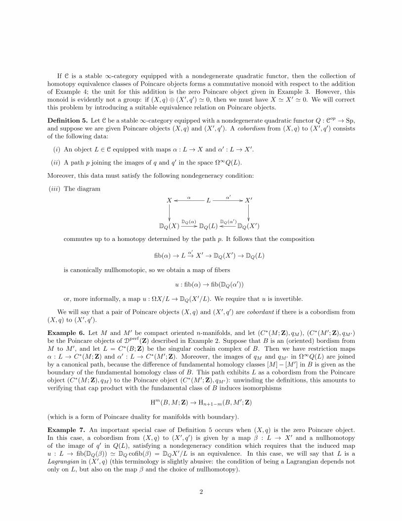
Definition 5. Let C be a stable∞-category equipped with a nondegenerate quadratic functor Q : Cop → Sp,and suppose we are given Poincare objects (X, q) and (X ′, q′). A cobordism from (X, q) to (X ′, q′) consistsof the following data:

(i) An object L ∈ C equipped with maps α : L→ X and α′ : L→ X ′.

(ii) A path p joining the images of q and q′ in the space Ω∞Q(L).

Moreover, this data must satisfy the following nondegeneracy condition:

(iii) The diagram

X

Lαoo α′

// X ′

DQ(X)

DQ(α) // DQ(L) DQ(X ′)DQ(α′)oo

commutes up to a homotopy determined by the path p. It follows that the composition

fib(α)→ Lα′

→ X ′ → DQ(X ′)→ DQ(L)

is canonically nullhomotopic, so we obtain a map of fibers

u : fib(α)→ fib(DQ(α′))

or, more informally, a map u : ΩX/L→ DQ(X ′/L). We require that u is invertible.

We will say that a pair of Poincare objects (X, q) and (X ′, q′) are cobordant if there is a cobordism from(X, q) to (X ′, q′).

Example 6. Let M and M ′ be compact oriented n-manifolds, and let (C∗(M ; Z), qM ), (C∗(M ′; Z), qM ′)be the Poincare objects of Dperf(Z) described in Example 2. Suppose that B is an (oriented) bordism fromM to M ′, and let L = C∗(B; Z) be the singular cochain complex of B. Then we have restriction mapsα : L → C∗(M ; Z) and α′ : L → C∗(M ′; Z). Moreover, the images of qM and qM ′ in Ω∞Q(L) are joinedby a canonical path, because the difference of fundamental homology classes [M ]− [M ′] in B is given as theboundary of the fundamental homology class of B. This path exhibits L as a cobordism from the Poincareobject (C∗(M ; Z), qM ) to the Poincare object (C∗(M ′; Z), qM ′): unwinding the definitions, this amounts toverifying that cap product with the fundamental class of B induces isomorphisms

Hm(B,M ; Z)→ Hn+1−m(B,M ′; Z)

(which is a form of Poincare duality for manifolds with boundary).

Example 7. An important special case of Definition 5 occurs when (X, q) is the zero Poincare object.In this case, a cobordism from (X, q) to (X ′, q′) is given by a map β : L → X ′ and a nullhomotopyof the image of q′ in Q(L), satisfying a nondegeneracy condition which requires that the induced mapu : L → fib(DQ(β)) ' DQ cofib(β) = DQX ′/L is an equivalence. In this case, we will say that L is aLagrangian in (X ′, q) (this terminology is slightly abusive: the condition of being a Lagrangian depends notonly on L, but also on the map β and the choice of nullhomotopy).

2

Example 8. In the situation of Definition 5, suppose that (X, q) and (X ′, q′) are both zero Poincareobjects. Then a cobordism from (X, q) to (X ′, q′) can be identified with an object L ∈ C together with apoint p ∈ Ω∞+1Q(L) which induces an equivalence L→ ΩDQ(L). In other words, a cobordism from (X, q)to (X ′, q′) can be identified with a Poincare object of C with respect to the shifted quadratic functor ΩQ.

Proposition 9. Let C be a stable ∞-category equipped with a nondegenerate quadratic functor Q. Therelation of cobordism is an equivalence relation on the collection of Poincare objects of (C, Q).

Proof. We first show that cobordism is reflexive. Let (X, q) be a Poincare object of (C, Q). Take L = X andlet α : L→ X and α′ : L→ X be the identity maps. Let p be the constant path between the images of q inΩ∞Q(L). Then (L,α, α′, p) is a cobordism from (X, q) to itself.

We next show that cobordism is symmetric. Let (X, q) and (X ′, q′) be Poincare objects of (C, Q), andsuppose we are given a diagram

Xα← L

α′

→ X ′

in C and a path joining the images of q and q′ in Ω∞Q(L). We claim that if this data is a cobordism from(X, q) to (X ′, q′), then it is also a cobordism from (X ′, q′) to (X, q). Condition (iii) of Definition 5 guaranteesthat the canonical map

u : fib(α)→ fib(DQ(α′)) ' DQ cofib(α′)

is an equivalence. We wish to show that the canonical map

v : fib(α′)→ fib(DQ(α)) ' DQ cofib(α)

is also an equivalence, or equivalently that

Σ(v) : cofib(α′)→ DQ fib(α)

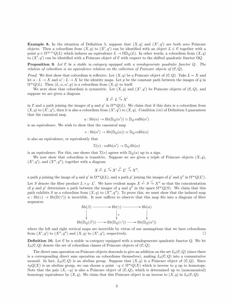
is an equivalence. For this, one shows that Σ(v) agrees with DQ(u) up to a sign.We now show that cobordism is transitive. Suppose we are given a triple of Poincare objects (X, q),

(X ′, q′), and (X ′′, q′′), together with a diagram

Xα← L

α′

→ X ′β← L′

β′

→ X ′′,

a path p joining the image of q and q′ in Ω∞Q(L), and a path p′ joining the images of q′ and q′′ in Ω∞Q(L′).

Let S denote the fiber product L ×X′ L′. We have evident maps Xγ← S

γ′

→ X ′′ so that the concatentationof p and p′ determines a path between the images of q and q′′ in the space Ω∞Q(S). We claim that thispath exhibits S as a cobordism from (X, q) to (X ′′, q′′). To prove this, we must show that the induced mapu : fib(γ) → fib(D(γ′)) is invertible. It now suffices to observe that this map fits into a diagram of fibersequences

fib(β) //

fib(γ) //

u

fib(α)

fib(DQ(β′)) // fib(DQ(γ′)) // fib(DQ(α′))

where the left and right vertical maps are invertible by virtue of our assumptions that we have cobordismsfrom (X ′, q′) to (X ′′, q′′) and (X, q) to (X ′, q′), respectively.

Definition 10. Let C be a stable ∞-category equipped with a nondegenerate quadratic functor Q. We letL0(C, Q) denote the set of cobordism classes of Poincare objects of (C, Q).

The direct sum operation on Poincare objects descends to give an addition on the set L0(C, Q) (since thereis a corresponding direct sum operation on cobordisms themselves), making L0(C, Q) into a commutativemonoid. In fact, L0(C, Q) is an abelian group. Suppose that (X, q) is a Poincare object of (C, Q). Sinceπ0Q(X) is an abelian group, we can choose a point −q ∈ Ω∞Q(X) which is inverse to q up to homotopy.Note that the pair (X,−q) is also a Poincare object of (C, Q), which is determined up to (noncanonical)homotopy equivalence by (X, q). We claim that this Poincare object is an inverse to (X, q) in L0(C, Q):

3

Proposition 11. In the above situation, we have (X, q) ⊕ (X,−q) = 0 in L0(C, Q). That is, there is acobordism from (X ⊕X, q ⊕−q) to the zero Poincare object.

Proof. By Example 7, we must show that there exists a Lagrangian β : L → X ⊕ X. For this, we takeL = X and β to be the diagonal map, and choose any path from the sum (q +−q) ∈ Ω∞Q(X) to the basepoint. The requisite nondegeneracy condition follows from our assumption that q induces an equivalenceX → DQX.

By virtue of the above result, we are now justified in referring to L0(C, Q) as the 0th L-group of the pair(C, Q).

Remark 12. Let M be a compact oriented manifold of dimension n, and let (C∗(M ; Z), qM ) as in Example6. Then (C∗(M ; Z), qM ) determines an element of L0(Dperf(Z), Q), and this element is an incarnation ofthe signature of the manifold M . (In fact, when n is divisible by 4 one can show that L0(Dperf(Z), Q) isisomorphic to Z and this invariant is precisely the signature). We will ultimately need a more refined versionof the signature invariant in order to describe the surgery classification of manifolds. However, this morerefined invariant will have the same basic flavor: it will live in a group L0(C, Q) for some quadratic functoron a stable ∞-category C, and the invariant associated to M will be some avatar of the stable homotopytype of M , equipped with its intersection product.

4

L-theory Spaces (Lecture 6)

February 3, 2011

Let C be a stable ∞-category equipped with a nondegenerate quadratic functor Q : Cop → Sp, whichwe regard as fixed throughout this lecture. We let B : Cop×Cop → Sp denote the polarization of Q, andD : Cop → C the corresponding duality functor. In the last lecture, we introduce the notion of a cobordismbetween two Poincare objects (X, q) and (X ′, q′) of C. We saw that cobordism is an equivalence relation anddefined L0(C, Q) to be the set of equivalence classes.

In this lecture, we would like to refine the invariant L0(C, Q). We will accomplish this by defining anL-theory space L(C, Q), with π0L(C, Q) = L0(C, Q).

We first describe an approximation to this L-theory space. We let Poinc(C, Q) denote a classifying spacefor Poincare objects of C. That is, Poinc(C, Q) is an ∞-category whose objects are Poincare objects (X, q)of C, where a morphism from (X, q) to (X ′, q′) is an isomorphism α : X → X ′ together with a path joiningq to the image of q′ in the space Ω∞Q(X). Poinc(C, Q) is an ∞-category in which every morphism isinvertible and therefore a Kan complex. We will simply refer to Poinc(C, Q) as a space. It is not the spacewe are looking for, because cobordant Poincare objects need not lie in the same connected component ofPoinc(C, Q).

Notation 1. Fix an integer n ≥ 0. We let Fn denote the collection of nonempty subsets of the set0, 1, . . . , n. We regard Fn as a partially ordered set with respect to inclusions. (It may be helpful to thinkof Fn as the partially ordered set of faces of the standard n-simplex ∆n.) Note that Fn has a largest element,given by the set [n] = 0, . . . , n.

Let C[n] denote the ∞-category of functors Fun(Fopn ,C) from Fopn into C. We define a functor

Q[n] : Cop[n] → Sp

by the formula Q[n](X) = lim←−S∈FnQ(X(S)).

Using the fact thatQ is quadratic, it follows immediately thatQ[n] is a quadratic functor. The polarizationof Q[n] is the functor B[n] given by

B[n](X,X′) = lim←−

S∈Fn

B(X(S), X ′(S)).

Proposition 2. The bilinear functor B[n] is representable. Its associated duality functor D[n] is describedby the formula

(D[n]X)(S) = lim←−T⊆S

D(X(T )).

Proof. For simplicity let us assume the existence of D[n] and show that it is characterized by the aboveformula (the existence is proven in essentially the same way). We will show that for each object C ∈ C, thereis a canonical homotopy equivalence of spectra

MorC(C, (D[n]X)(S)) ' lim←−T⊆S

MorC(C,D(X(T ))).

1

Let Y : Fopn → C be given by the formula

Y (T ) =

C if T ⊆ S0 otherwise.

Then

MorC(C, (D[n]X)(S)) ' MorC[n](Y,D[n]X)

' B[n](Y,X)

' lim←−T

B(Y (T ), X(T ))

' lim←−T⊆S

B(C,X(T ))

' lim←−T⊆S

MorC(C,DX(T ))

' MorC(C, lim←−T⊆S

X(T )).

Proposition 3. The bilinear functor B[n] is nondegenerate.

Proof. We must show that the canonical map id → D2n is an equivalence from C[n] to itself. Fix an object

X ∈ C[n]. We compute

(D2[n]X)(S) ' lim←−

T⊆SD((D[n]X)(T ))

' D lim−→T⊆S

(D[n]X)(T )

' D lim−→T⊆S

lim←−U⊆T

DX(U)

' D2 lim←−T⊆S

lim−→U⊆T

X(U)

' lim←−T⊆S

lim−→U⊆T

X(U).

We wish to show that the canonical map

X(S)→ lim←−T⊆S

lim−→U⊆T

X(U)

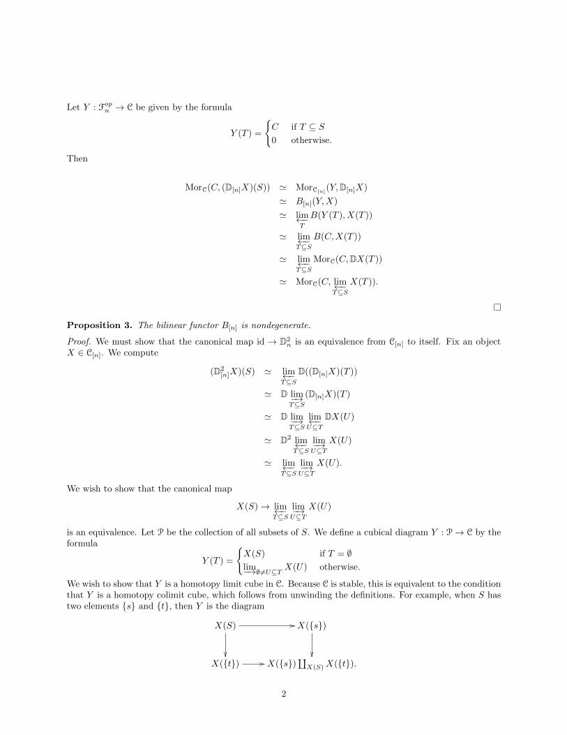
is an equivalence. Let P be the collection of all subsets of S. We define a cubical diagram Y : P→ C by theformula

Y (T ) =

X(S) if T = ∅lim−→∅6=U⊆T X(U) otherwise.

We wish to show that Y is a homotopy limit cube in C. Because C is stable, this is equivalent to the conditionthat Y is a homotopy colimit cube, which follows from unwinding the definitions. For example, when S hastwo elements s and t, then Y is the diagram

X(S) //

X(s)

X(t) // X(s)

∐X(S)X(t).

2

Example 4. Let n = 1. Then an object X of C[1] consists of a diagram

X(0)← X([1])→ X(1)

in C. The spectrum Q[2](X) is given by the homotopy fiber product

Q(X(0))×Q(X([1])) Q(X(1)).

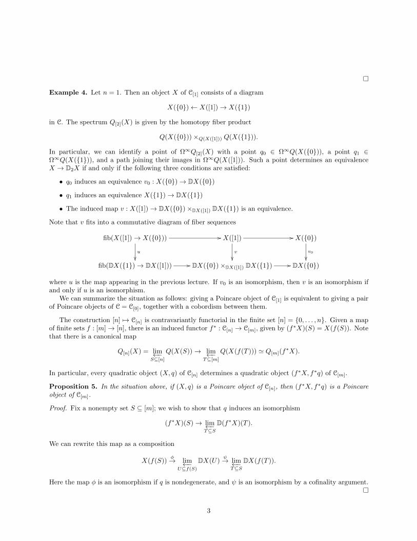
In particular, we can identify a point of Ω∞Q[2](X) with a point q0 ∈ Ω∞Q(X(0)), a point q1 ∈Ω∞Q(X(1)), and a path joining their images in Ω∞Q(X([1])). Such a point determines an equivalenceX → D2X if and only if the following three conditions are satisfied:

• q0 induces an equivalence v0 : X(0)→ DX(0)

• q1 induces an equivalence X(1)→ DX(1)

• The induced map v : X([1])→ DX(0)×DX([1]) DX(1) is an equivalence.

Note that v fits into a commutative diagram of fiber sequences

fib(X([1])→ X(0)) //

u

X([1])

v

// X(0)

v0

fib(DX(1)→ DX([1])) // DX(0)×DX([1]) DX(1) // DX(0)

where u is the map appearing in the previous lecture. If v0 is an isomorphism, then v is an isomorphism ifand only if u is an isomorphism.

We can summarize the situation as follows: giving a Poincare object of C[1] is equivalent to giving a pairof Poincare objects of C = C[0], together with a cobordism between them.

The construction [n] 7→ C[n] is contravariantly functorial in the finite set [n] = 0, . . . , n. Given a mapof finite sets f : [m]→ [n], there is an induced functor f∗ : C[n] → C[m], given by (f∗X)(S) = X(f(S)). Notethat there is a canonical map

Q[n](X) = lim←−S⊆[n]

Q(X(S))→ lim←−T⊆[m]

Q(X(f(T ))) ' Q[m](f∗X).

In particular, every quadratic object (X, q) of C[n] determines a quadratic object (f∗X, f∗q) of C[m].

Proposition 5. In the situation above, if (X, q) is a Poincare object of C[n], then (f∗X, f∗q) is a Poincareobject of C[m].

Proof. Fix a nonempty set S ⊆ [m]; we wish to show that q induces an isomorphism

(f∗X)(S)→ lim←−T⊆S

D(f∗X)(T ).

We can rewrite this map as a composition

X(f(S))φ→ lim←−U⊆f(S)

DX(U)ψ→ lim←−T⊆S

DX(f(T )).

Here the map φ is an isomorphism if q is nondegenerate, and ψ is an isomorphism by a cofinality argument.

3

For each n ≥ 0, let Poinc(C, Q)n denote a classifying space for Poincare objects of (C[n], Q[n]). Itfollows from the preceding result that a map of finite sets f : [m] → [n] induces a map of classifyingspaces Poinc(C, Q)n → Poinc(C, Q)m. Restricting our attention to order-preserving maps f , we see thatPoinc(C, Q)• has the structure of a simplicial space.

Definition 6. We define L(C, Q) to be classifying space of the simplicial space Poinc(C, Q)•. We will referto L(C, Q) as the L-theory space of (C, Q).

Remark 7. The set π0L(C, Q) can be identified with the quotient of π0 Poinc(C, Q) by the equivalencerelation generated by the image of π0 Poinc(C, Q)1 in π0 Poinc(C, Q)× π0 Poinc(C, Q). Using Example 4, wesee that this is exactly the relation of cobordism defined in the previous lecture. It follows that we have acanonical isomorphism

π0L(C, Q) ' L0(C, Q).

All of the constructions of this lecture are compatible with the formation of direct sums of Poincareobjects. It follows that the L-theory space L(C, Q) inherits a monoid structure, which is commutative andassociative up to coherent homotopy: that is, L(C, Q) is an E∞-space. Moreover, we saw in the last lecturethat the induced monoid structure on π0L(C, Q) ' L0(C, Q) is actually an abelian group structure. In otherwords, L(C, Q) is a grouplike E∞-space, and therefore an infinite loop space.

Remark 8. We will later construct a nonconnective delooping of L(C, Q).

Definition 9. For n ≥ 0, we let Ln(C, Q) denote the homotopy group πnL(C, Q). We will refer to Ln(C, Q)as the nth L-group of (C, Q).

We will return to the study of these higher L-groups in the next lecture.

4

Simplicial Spaces (Lecture 7)

February 6, 2011

Let C be a stable∞-category equipped with a nondegenerate quadratic functor Q : Cop → Sp. In the lastlecture, we defined an L-theory space L(C, Q), whose path components comprise the abelian group L0(C, Q)of Lecture 5. We would like to understand the homotopy type L(C, Q) better. For example, we might askfor an interpretation of the higher homotopy groups Ln(C, Q) = πnL(C, Q).

By definition, L(C, Q) is given to us as the geometric realization of a simplicial space Poinc(C, Q)•. Ingeneral, it is not easy to describe the homotopy groups of a geometric realization even if the homotopygroups of the indiviual terms are well-understood (for example, it is hard to describe the homotopy groupsof the geometric realization of the simplicial set ∂∆3).

For a general simplicial space X•, there are two face maps d0, d1 : X1 → X0 which induce a mapπ0(X1) → π0X0 × π0X0. The image of this map is a relation R on π0X0, and the quotient of π0X0 by theequivalence relation generated by R can be identified with π0|X•|. However, in our case R is the relationof cobordism of Poincare objects, which is already an equivalence relation. This is a special feature ofPoinc(C, Q)• which makes the homotopy group π0L(C, Q) easier to compute. We would like to generalizethis observation.

We begin by introducing some notation.

Definition 1. Let ∆ denote the category of combinatorial simplices: that is, nonempty finite linearlyordered sets of the form 0, . . . , n. In this lecture, we will identify the objects of ∆ with the correspondingsimplicial sets ∆0,∆1, · · · . A simplicial space is a functor from ∆op to the ∞-category of spaces. If X is asimplicial space, we will denote the individual spaces of X by X(∆0), X(∆1), and so forth.

If X is a simplicial space, then X determines a functor from the ordinary category of simplicial sets intothe ∞-category of spaces, given by

K 7→ lim←−σ:∆n→K

X(∆n).

We will denote this functor by K 7→ X(K). (More abstractly: we regard X as a functor defined on allsimplicial sets, rather than just standard simplices, by taking a right Kan extension.)

Remark 2. We can identify X(K) with the space of maps from K to X in the ∞-category of simplicialspaces (where we regard K as a simplicial space by endowing it with the discrete topology in each degree).

Definition 3. Let f : X → Y be a map of simplicial spaces. We will say that f is a Kan fibration if thefollowing condition is satisfied: for 0 ≤ i ≤ n, the map

X(∆n)→ X(Λni )×Y (Λni ) Y (∆n)

is surjective on connected components (here the fiber product denotes a homotopy fiber product). We willsay that f is a trivial Kan fibration if, for each n ≥ 0, the map

X(∆n)→ X(∂∆n)×Y (∂∆n) Y (∆n).

We will say that a simplicial space X satisfies the Kan condition if the map X → ∗ is a Kan fibration, where∗ denotes the constant simplicial space with value equal to a single point.

1

Remark 4. When we restrict our attention to simplicial sets (which we regard as a special case of simplicialspaces), Definition 3 recovers the usual notion of Kan fibration, trivial Kan fibration, and Kan complex.

If X is a simplicial space satisfying the Kan condition, then the surjectivity of the map π0X(∆2) →π0X(Λ2

1) guarantees that the image of π0X(∆1) is an equivalence relation on π0X(∆0). Since we know thatthe latter condition holds for Poinc(C, Q)•, we are naturally led to conjecture the following:

Theorem 5. The simplicial space Poinc(C, Q)• satisfies the Kan condition.

We will prove Theorem 5 later this week. The remainder of this lecture is devoted to exploring someconsequences of Theorem 5.

Recall that if f : X → Y is a trivial Kan fibration of simplicial sets, then f induces a homotopy equivalenceof geometric realizations |X| → |Y |. This generalizes to simplicial spaces:

Proposition 6. Let f : X → Y be a trivial Kan fibration of simplicial spaces. Then the induced map|X| → |Y | is a homotopy equivalence.

Proof. The category Set∆ of simplicial sets is a model for the ∞-category of spaces. We may thereforechoose a simplicial object X of the category of simplicial sets representing X, and a simplicial object Yof the category of simplicial sets representing Y , such that f is modelled by a map of bisimplicial setsf : X → Y . Without loss of generality, we may assume that X and Y are Reedy fibrant and that f is aReedy fibration. Then each of the maps

X(∆n)→ X(∂∆n)×Y (∂∆n) Y (∆n)

is modelled by a Kan fibration of simplicial sets

X(∆n)→ X(∂∆n)×Y (∂∆n) Y (∆n)

Our assumption on f guarantees that this map is surjective on connected components. Since it is a Kanfibration, it is surjective on simplices of every dimension. In other words, we deduce that for each m ≥ 0,the map of simplicial sets

Xm → Y m

is a trivial Kan fibration. In particular, the map of bisimplicial sets f : X → Y is a levelwise homotopyequivalence in the “horizontal” direction, and so induces a homotopy equivalence after geometric realization.

Proposition 7. Let Y be a simplicial space. Then there exists a simplicial set X and a trivial Kan fibrationf : X → Y .

Proof. We successively build n-skeletal simplicial sets sknX and maps sknX → Y such that the maps

sknX(∆m)→ (sknX)(∂∆m)×Y (∂∆m) Y (∆m)

are surjective on connective components for m ≤ n. Assume that skn−1X has already been constructed.Let S be the set of connected components of the fiber product

(skn−1X)(∂∆n)×Y (∂∆n) Y (∆n).

and let sknX be the simplicial set obtained from skn−1X by adjoining one nondegenerate n-simplex for everyelement of S (with the obvious attaching maps). There is an evident map of simplicial spaces sknX → Yhaving the desired properties.

2

Let Y be a simplicial space satisfying the Kan condition, and suppose that we wish to describe thehomotopy groups of the geometric realization |Y |. Choose a trivial Kan fibration X → Y , where X is asimplicial set. Then the map |X| → |Y | is a homotopy equivalence, so the homotopy groups of |Y | are thesame as the homotopy groups of |X|. Moreover, since X → Y is a Kan fibration, the simplicial set X alsosatisfies the Kan condition: that is, it is a Kan complex in the usual sense. Let us fix a base point x ofX(∆0) (which determines a base point in Y (∆0)) and compute all homotopy groups with respect to thatbase point. If K is a simplicial set with a simplicial subset K0, let Y (K,K0) denote the homotopy fiber ofthe map Y (K)→ Y (K0) (over the point determined by the base point), and define X(K,K0) similarly.

Because X is a Kan complex, there is a simple combinatorial recipe for extracting the homotopy groupsπn|X|. Let us recall how this goes. Every class in πn|X| is represented by a point η ∈ X(∆n, ∂∆n). LetK ⊆ ∂∆n+1 be the subset obtained by removing the interiors of two faces, so that we have a canonicalbijection

X(∂∆n+1,K)→ X(∆n, ∂∆n)×X(∆n, ∂∆n).

A pair of elements η, η′ ∈ X(∆n, ∂∆n) determine the same element in πn|X| if and only if the correspondingelement of X(∂∆n+1,K) can be lifted to X(∆n+1,K).

Since X → Y is a trivial Kan fibration, the map

φ : X(∆n, ∂∆n)→ Y (∆n, ∂∆n).

is surjective on connected components: that is, every element of π0Y (∆n, ∂∆n) comes from a point η ∈X(∆n, ∂∆n). Suppose we are given a pair of points of Y (∆n, ∂∆n), given by the images of elements η, η′ ∈X(∆n, ∂∆n). This pair of points determines a point ζ ∈ X(∂∆n+1,K) having image ζ0 ∈ Y (∂∆n+1,K).Since the map

X(∆n+1)→ X(∂∆n+1)×Y (∂∆n+1) Y (∆n+1)

is surjective on connected components, we deduce that ζ0 lifts to a point of Y (∆n+1) if and only if ζ lifts toa point of X(∆n+1). We have proven the following:

Proposition 8. Let Y be a simplicial space satisfying the Kan condition, and choose a base point y ∈ Y (∆0)(so that we can regard Y as a simplicial pointed space). Then πn|Y | can be identified with the quotient ofthe set π0Y (∆n, ∂∆n) by the following equivalence relation: two homotopy classes [η], [η′] ∈ π0Y (∆n, ∂∆n)represent the same class in πn|Y | if and only if the corresponding point of Y (∂∆n+1,K) lifts to a point ofY (∆n+1).

Let us now apply this analysis to the case of interest, where Y is the simplicial space Poinc(C, Q)•.Unwinding the definitions, we see that Y (∆n, ∂∆n) is a classifying space for Poincare objects (X, q) of C[n]

(using the notation of the previous lecture) such that X(S) ' 0 for all proper subsets S ⊆ [n]. In this case,X is determined by a single object C = X([n]) ∈ C. Moreover, we have

Q[n](X) = lim←−S

Q(X(S)) = lim←−S

Q(C) if S = [n]

0 otherwise.

The relevant diagram is parametrizes by partially ordered set of faces of an n-simplex, taking the value 0 onevery proper face. Consequently, the limit in question is given by ΩnQ(C). We can summarize our analysisas follows:

(∗) Let Y = Poinc(C, Q)•. Then Y (∆n, ∂∆n) is a classifying space for Poincare objects of (C,ΩnQ).

Now suppose we are given two Poincare objects for (C,ΩnQ). They determine a point of Y (∂∆n+1):that is, a functor from the partially ordered set of all nonempty proper subsets of [n+ 1] into C. Moreover,this functor vanishes identically except on two subsets of [n+ 1] of cardinality n. Unwinding the definitions,we see that lifting this data to a Poincare object of C[n+1] is equivalent to specifying a cobordism betwee thecorresponding Poincare object of (C,ΩnQ). We have proven the following:

3

Theorem 9. The abelian group Ln(C, Q) = πnL(C, Q) is canonically isomorphic to L0(C,ΩnQ).

We close with a result that will be needed in the next lecture:

Proposition 10. Let X → Yu→ Z be a fiber sequence of simplicial spaces. Suppose that u is a Kan fibration.

Then|X| → |Y | → |Z|

is a fiber sequence of spaces.

Proof. Choose a trivial Kan fibration f : Z ′ → Z, where Z ′ is a simplicial set (and choose a base point of Z ′

lying over the chosen base point of Z). Now choose a trivial Kan fibration g : Y ′ → Y ×Z Z ′, where Y ′ is asimplicial set. The canonical map Y ′ → Y is a composition of g with a pullback of f , and therefore a trivialKan fibration. Let X ′ be the fiber of the map of simplicial sets Y ′ → Z ′. The canonical map X ′ → X is apullback of g and therefore a trivial Kan fibration. We have a commutative diagram of fiber sequences

X ′ //

Y ′ //

Z ′

X // Y // Z

where the vertical maps are trivial Kan fibrations, and therefore induce homotopy equivalences after geo-metric realization. It will therefore suffice to prove that the sequence of spaces

|X ′| → |Y ′| → |Z ′|

is a fiber sequence. Since these are simplicial sets, it suffices to prove that the map Y ′ → Z ′ is a Kanfibration. This map is given by the composition of g (a trivial Kan fibraation) with the projection mapu′ : Y ×Z Z ′ → Z ′. It will therefore suffice to show that u′ is a Kan fibration (of simplicial spaces). This isclear, since u′ is a pullback of the Kan fibration u.

4

Localization (Lecture 8)

February 9, 2011

Let C be a stable∞-category equipped with a nondegenerate quadratic functor Q : Cop → Sp. In the lastlecture, we asserted without proof that the simplicial space Poinc(C, Q)• satisfies the Kan condition. Ourgoal in this lecture is to formulate a generalization of this assertion, which we will prove in the next lecture.

We begin with some generalities. Let J be an ∞-category. We say that J is filtered if it satisfies thefollowing conditions:

• J is nonempty.

• For every pair of objects X,Y ∈ J, there is a third object Z ∈ J and a pair of maps X → Z ← Y .

• For every pair of objects X,Y ∈ J and every map of spaces Sn → MapJ(X,Y ), there is a map g : Y → Zsuch that the composite map Sn → MapJ(X,Y )→ MapJ(X,Z) is nullhomotopic.

Let C be an ∞-category. By a filtered diagram in C we will refer to a functor Jop → C, where J is afiltered ∞-category. We will denote a filtered diagram in C by (Xα), where each Xα is an object of C. Thecollection of filtered diagrams in C can be organized into an ∞-category Pro(C), where morphism spaces aregiven by

MapPro(C)((Xα), (Yβ)) = lim←−β

lim−→α

MapC(Xα, Yβ).

We refer to the objects of Pro(C) as Pro-objects of C.We will identify C with a full subcategory of Pro(C) (each object X ∈ C determines a filtered diagram (X)

indexed by the one-point∞-category ∗). For every filtered diagram (Xα), we can identify the correspondingobject of Pro(C) with the (homotopy) limit lim←−Xα in Pro(C). We can think of Pro(C) as the ∞-categoryobtained from C by formally adjoining limits of filtered diagrams. In fact, Pro(C) has the following universalproperty: if D is an ∞-category which admits filtered limits, then the ∞-category of functors Pro(C) → D

which preserve filtered limits is equivalent to the ∞-category of functors C→ D.

Remark 1. It is not necessary to allow arbitrary filtered ∞-categories in the definition of Pro(C). One canshow that every filtered diagram is equivalent (in the∞-category Pro(C)) to a diagram indexed by a filteredpartially ordered set.

Remark 2. If C is a stable ∞-category, then the ∞-category Pro(C) is also stable.

Suppose that C is a stable∞-category and let C0 be a stable subcategory of C (that is, a subcategory closedunder the formation of fibers and cofibers). We will say that a map f : X ′ → X in C is a C0-equivalence if thecofiber cofib(f) belongs to C0. If we regard X as fixed, then the collection of all C0-equivalences fα : Xα → Xforms a filtered ∞-category (in fact, it is an ∞-category which admits finite limits). Consequently, we canregard (Xα) as a Pro-object of C. We will denote this pro-object by I(X) ∈ Pro(C).

Definition 3. Let C be a (small) stable ∞-category and let C0 be a stable subcategory of C. We let C /C0

denote the full subcategory of Pro(C) spanned by objects of the form I(X), where X ∈ C.

1

It is not difficult to see that the construction X 7→ I(X) commutes with finite limits. From this, one candeduce that C /C0 is closed under passing to fibers in Pro(C). It follows that C /C0 is a stable subcategoryof Pro(C).

The following result justifies our notation:

Proposition 4. Let D be a stable ∞-category. Then composition with the functor I : C → C /C0 inducesan equivalence from the ∞-category of exact functors f : C /C0 → D, to the ∞-category of exact functorsF : C→ D such that F |C0 is trivial.

Proof. Note that if X ∈ C0, then the filtered ∞-category of C0-equivalences X ′ → X has an initial object(namely, the map 0 → X), so that I(X) ' 0. It follows that for any exact functor f : C /C0 → D, thecomposition F = f I is an exact functor from C to D which annihilates C0.

We now produce an inverse to the preceding construction. Embed D in a stable ∞-category D whichadmits filtered limits (for example, we can take D = Pro(D)). Let F : C → D be an exact functor whichannhilates C0. Then F extends to a functor F : Pro(C)→ D which commutes with filtered limits. For eachX ∈ C, we have a canonical map I(X) → X in Pro(C), hence a map u : F (I(X)) → F (X) in D. Thecofiber of the map I(X) → X is a filtered limit of objects of C0. Since F annihilates C0 and F commuteswith filtered limits, we deduce that u is invertible: that is, we can write F = F I. In particular, F carriesI(C) = C /C0 into the subcategory D ⊆ D. Let us denote this restricted functor by f : C /C0 → D; thenF = f I as desired.

Now suppose that C is equipped with a nondegenerate quadratic functor Q. We can extend Q to a functorQ : Pro(C)op → Sp by the formula

Q((Xα)) = lim−→α

Q(Xα).

It is easy to see that Q is a quadratic functor on Pro(C), whose polarization B is given by the formula

B((Xα), (Yβ)) = lim−→α,β

B(Xα, Yβ)

where B denotes the polarization of Q.

Definition 5. Let C be a stable∞-category equipped with a nondegenerate quadratic functor Q : Cop → Sp.Let B be the polarization of Q and let D denote the corresponding duality functor. We will say that Q iscompatible with a stable subcategory C0 if the duality functor D carries C0 to itself. In this case, Q′ = Q|Cop0is a nondegenerate quadratic functor on C0, having polarization B′ = B|Cop0 ×C

op0 and duality functor

D′ = D|C0.

In the above situation, the composition

CD→ Cop → (C /C0)op

annihilates the subcategory C0, and therefore factors (in an essentially unique way) as a composition

C→ C /C0D′′

→ (C /C0)op.

Using the fact that D has order 2, we deduce easily that D′′ also has order 2; in particular, it is a contravariantequivalence of C /C0 with itself.

Proposition 6. In the above situation, the quadratic functor Q on Pro(C) restricts to a nondegeneratequadratic functor Q′′ on C /C0, whose duality functor is given by D′′.

2

Proof. Let X be an object of C and write I(X) = (Xα). Note that if Z ∈ C0, then any map I(X) → Zin Pro(C) is nullhomotopic: such a map must factor through some Xα, but the fiber F of the induced mapXα → Z also belongs to the filtered system (Xα) (and composition F → Xα → Z is nullhomotopic).

Let Y ∈ C and write I(Y ) = (Yβ). The above argument shows that

MorPro(C)(I(X), Yβ)→ MorPro(C)(I(X), Y )

for each index β, so that MorPro(C)(I(X), I(Y )) ' MorPro(C)(I(X), Y ). We therefore obtain a canonicalhomotopy equivalence

MorPro(C)(I(X),D′′I(Y )) ' MorPro(C)(I(X), I(DY ))

' MorPro(C)(I(X),DY )

' lim−→α

MorPro(C)(Xα,DY )

' lim−→α

B(Xα, Y ).

For every index β, the cofiber Z of the map Yβ → Y belongs to C0, so that D(Z) ∈ C0. It follows that

lim−→α

B(Xα, Z) ' MorPro(C)(I(X),D(Z)) ' 0,

so thatlim−→α

B(Xα, Y ) ' lim−→α

B(Xα, Yβ).

Passing to the limit over β, we get

MorPro(C)(I(X),D′′I(Y )) ' lim−→α

B(Xα, Y ) ' lim−→α,β

B(Xα, Yβ) = B(I(X), I(Y )),

so that D′′ is the duality functor associated to the bilinear pairing B restricted to C /C0.

Let (X, q) be a quadratic object of C. Then q determines a point q′′ ∈ Ω∞Q(I(X)), so that (I(X), q′′)can be viewed as a quadratic object of (C /C0, Q

′′). We have just verified that the functor I : C → C /C0

interchanges the duality functors induced by Q and Q′′ respectively. It follows that if (X, q) is a Poincareobject of (C, Q), then (I(X), q′′) is a Poincare object of (C /C0, Q

′′). This construction determines a map ofclassifying spaces

Poinc(C, Q)→ Poinc(C /C0, Q′′)

whose fiber (over the zero object) can be identified with Poinc(C0, Q′). Applying the same reasoning to the

∞-categories C[n] for n ≥ 0, we obtain a fiber sequence of simplicial spaces

Poinc(C0, Q′)• → Poinc(C, Q)•

φ→ Poinc(C /C0, Q′′)•

We will prove the following result in the next lecture:

Theorem 7. Let C be a stable ∞-category equipped with a nondegenerate quadratic functor Q, and let C0 bea stable subcategory of C which is closed under duality. Then the map φ : Poinc(C, Q)• → Poinc(C /C0, Q

′′)•is a Kan fibration of simplicial spaces.

Corollary 8. Let C be a stable ∞-category equipped with a nondegenerate quadratic functor Q. Then thesimplicial space Poinc(C, Q)• satisfies the Kan condition.

Proof. Apply Theorem 7 in the special case C0 = C.

3

Corollary 9. In the situation of Theorem 7, we have a fiber sequence of L-theory spaces

L(C0, Q′)→ L(C, Q)→ L(C /C0, Q

′′),

and therefore a long exact sequence of abelian groups

· · · → L1(C /C0, Q′′)→ L0(C0, Q

′)→ L0(C, Q)→ L0(C /C0, Q′′).

Proof. Combine Theorem 7 with the result stated at the end of the previous lecture.

4

Proof of the Kan Property (Lecture 9)

February 11, 2011

Let C be a stable ∞-category equipped with a nondegenerate quadratic functor Q : Cop → Sp. Let B bethe polarization of Q and D the associated duality functor. Our goal in this lecture is to prove the following:

Theorem 1. Let C0 ⊆ C be a stable subcategory which is closed under D. Then the canonical mapPoinc(C, Q)• → Poinc(C /C0, Q

′′)• is a Kan fibration of simplicial spaces (here Q′′ is the quadratic func-tor on C /C0 defined in the previous lecture).

Before giving the proof, we embark on two digressions.

Notation 2. We let Lagr(C, Q) denote the full subcategory of C[1] spanned by those diagrams

X0 ← X01 → X1

where X1 = 0, and endow Lagr(C, Q) with the quadratic functor QLagr given by the restriction of Q[1].

Lemma 3. We have L0(Lagr(C, Q), QLagr) = 0.

Remark 4. Lemma 3 can be regarded as an algebraic analogue of the following topological fact: for anytopological space X with a base point x ∈ X, the space of paths in X ending in x is contractible.

Proof. Fix a Poincare object (X, q) of Lagr(C, Q), so that X is given by a diagram

X0 ← X01 → 0

Let L ∈ Lagr(C, Q) be the diagramX01 ← X01 → 0.

There is a canonical map L→ X. Note that QLagr(L) = Q(0)×Q(X01)Q(X01) ' 0, so that the restriction ofq to L is canonically nullhomotopic. A simple calculation shows that L is a Lagrangian in X, so that (X, q)represents 0 ∈ L0(Lagr(C, Q), QLagr).

We now discuss the classification of quadratic objects of (C, Q) which are not necessarily Poincare. Let usbegin with an example for motivation. Let C = Dperf(Z), let B be the symmetric bilinear functor associatedto the duality functor

P• 7→ Hom(P•,Z[−n])

and let Q(X) = B(X,X)hΣ2 be the associated quadratic functor. Let M be a compact oriented n-manifoldwith boundary. Then we have an intersection form

C∗(M,∂M)⊗ C∗(M,∂M)[M ]→ Z[−n]

which determines a quadratic object (C∗(M,∂M), qM ) of C. If M is a closed manifold, then this objectis Poincare. In general it is not: the point qM determines a map C∗(M,∂M) → DC∗(M,∂M) ' C∗(M),which can be identified with the standard inclusion of relative cochains into cochains. The cofiber of this map

1

is C∗(∂M). Note that this cofiber is itself described as a complex of cochains on a manifold (of dimensionn−1 rather than n), and so determines a Poincare object of (C,ΣQ). We will now show that this is a generalphenomenon.

So far, we have not used the full strength of our assumption that Q is a quadratic functor. The nextresult remedies this:

Proposition 5. Suppose we are given a fiber sequence

X ′ → X → X ′′

in C. Then Q(X ′′) is the total homotopy fiber of the diagram

Q(X) //

Q(X ′)

B(X ′, X) // B(X ′, X ′)

In other words, Q(X ′′) is equivalent to the fiber of the map

Q(X ′)×B(X′,X′) B(X ′, X).

Remark 6. Let us state this result more informally. Think of Q(X) as a spectrum parametrizing “quadraticforms” on X. The Proposition addresses the following question: given a quadratic form on X, when does itdescend to X ′′ = X/X ′? An obvious necessary condition is that it should vanish on X ′. This implies thatthe associated bilinear form vanishes on X ′. But we need a bit more: namely, to know that X ′ lies in thekernel of the associated bilinear form.

Proof. We wish to show that for every quadratic functor Q on C, the triangle

Q(X ′′)→ Q(X)→ Q(X ′)×B(X′,X′) B(X,X ′)

is a fiber sequence. We have a fiber sequence of functors

Q0(Z)→ Q(Z)→ B(Z,Z)hΣ2 .

It therefore suffices to prove the result after replacing Q by Q0 or B(Z,Z)hΣ2 . In the first case, the polariza-tion of Q0 vanishes and the desired result follows from the fact that Q0 is exact. Let us therefore assume thatQ(Z) = B(Z,Z)hΣ2 . Since B is exact in each variable, we can identify B(X ′′, X ′′) with the total homotopyfiber of the diagram

B(X,X) //

B(X,X ′)

B(X ′, X) // B(X ′, X ′).

In other words, B(X ′′, X ′′) is the fiber of the map

B(X,X)→ B(X,X ′)×B(X′,X′) B(X ′, X) ' (B(X,X ′)×B(X ′, X))×B(X′,X′)×B(X′,X′) B(X ′, X ′).

Taking homotopy fixed points with respect to Σ2, we get a fiber sequence

Q(X ′′)→ Q(X)→ B(X,X ′)×B(X′,X′) Q(X ′).

2

Let us rewrite the fiber sequence of Proposition 5 as

Q(X ′)×B(X′,X′) B(X ′, X)→ ΣQ(X ′′)→ ΣQ(X).

Suppose that (Y, q) is a quadratic object of (C, Q). There is a canonical point η ∈ Ω∞B(Y,DY ) (cor-responding to the identity map from Y to itself). Then q determines a point of Ω∞B(Y, Y ), which is theimage of η under the map B(Y,DY )→ B(Y, Y ) for some essentially unique map u : Y → DY . Form a fiber

sequence Yu→ D(Y ) → D(Y )/Y . Then the pair (q, η) determines a point of Ω∞(Q(Y ) ×B(Y,Y ) B(Y,DY ).

According to the above analysis, this is the 0th space of the fiber of the map of spectra

ΣQ(D(Y )/Y )→ ΣQ(DY ).

In particular, q determines a quadratic object of (C,ΣQ), which we will denote by (DY/Y, q).The point q determines a map

v : DY/Y → ΣD(DY/Y ) ' Σ fib(D2(Y )→ DY ) ' Σ fib(u) ' cofib(u) = DY/Y.

Unwinding the definitions, one sees that this is the identity map (up to a sign). Consequently, (D(Y )/Y, q) isa Poincare object of (C,ΣQ). We have a canonical map w : D(Y )→ D(Y )/Y , and a canonical nullhomotopyof the image of q in Q(D(Y )). This data determines a map

D(Y )→ (ΣD)(cofib(W )) ' ΣDΣY ' ΣΩD(Y ) ' D(Y ),

which is also the identity map (up to sign). Consequently, we can regard D(Y ) as a Lagrangian in (D(Y )/Y, q).We can summarize our discussion as follows:

(∗) Given a quadratic object (Y, q) of (C, Q), we can construct a Poincare object (D(Y )/Y, q) of (C,ΣQ)and a Lagrangian D(Y ) in (D(Y )/Y, q).

Remark 7. The converse to (∗) is true as well: given a Poincare object (Z, q) in (C, Q) and a Lagrangianf : L→ Z, we can equip the fiber fib(f) with the structure of a quadratic object of (C, Q).

Let us now suppose that C0 ⊆ C is a stable subcategory which is closed under duality. Suppose we aregiven a quadratic object (Y, q) of (C, Q) whose image in C /C0 is a Poincare object. Then the canonical mapu : Y → D(Y ) becomes invertible in C /C0, so the cofiber cofib(u) = D(Y )/Y belongs to C0. Consequently,the above construction produces a Poincare object (D(Y )/Y, q) of (C0,ΣQ

′) (where Q′ = Q|C0). Supposethat this Poincare object is nullcobordant: that is, we can choose a Lagrangian L→ D(Y )/Y in (C0,ΣQ

′).Then (D(Y )/Y, q) has two Lagrangians in the∞-category C: L and D(Y ). Each of these provides a cobordismof (D(Y )/Y, q) with the zero object. We have seen that cobordisms can be composed: if we compose thesecobordisms, we obtain a cobordism L×D(Y )/Y D(Y ) from the zero Poincare object of (C,ΣQ) to itself. Sucha cobordism can be regarded as a Poincare object (Y ′, q′) of (C,ΩΣQ) = (C, Q). Moreover, since L vanishesin C /C0, we note that (Y ′, q′) and (Y, q) determine the same quadratic object of C /C0.

Remark 8. Let (Y0, q0) be any Poincare object of C /C0. By construction, we can always lift (Y0, q0) to aquadratic object (Y, q) of C. The above discussion shows that we can adjust (Y, q) to be a Poincare objectof C if and only if a certain obstruction in L0(C0,ΣQ

′) vanishes. One we have proven the theorem, we canidentify this obstruction with the image of (Y0, q0) under the boundary map

π1L(C /C0,ΣQ′′)→ π0L(C0,ΣQ

′)

determined by the fiber sequence of spaces

L(C0,ΣQ′)→ L(C,ΣQ)→ L(C /C0,ΣQ

′′).

3

We now turn to the proof of Theorem 1. We must show that every point η of

Poinc(C /C0, Q′′)•(∆

n)×Poinc(C /C0,Q′′)•(Λni ) Poinc(C, Q)•(Λ

ni )

can be lifted (up to homotopy) to a point of Poinc(C, Q)•(∆n). The point η determines a Poincare object

(X0, q0) of (C /C0)[n]. Here we think of X0 as a contravariant functor from the collection of nonempty subsetsof 0, . . . , n into C /C0. Let σ = [n] = 0, . . . , n and let τ = [n] − i ⊆ σ. Then η determines objectsX(S) ∈ C lifting X0(S) for S /∈ σ, τ, together with a point of

q1 ∈ Ω∞ lim←−S/∈σ,τ

Q(X(S))

which is nondegenerate and compatible with q0. Using the construction of C /C0 and Q′′, we can extendX to a functor defined on all nonempty subsets of [n] and q1 to a point q ∈ Ω∞Q[n](X) (compatible withq0). What is not clear is that (X, q) is a Poincare object of (C[n], Q[n]). The point q determines a mapX → D[n](X), which may fail to be invertible when evaluated at σ and τ .

Let D be the full subcategory of C[n] spanned by those functors Z such that Z(S) ' 0 for S /∈ σ, τ,and Z(σ), Z(τ) ∈ C0. We can identify objects of D with morphisms Z(σ) → Z(τ) in C0, and so have anequivalence of ∞-categories D ' Lagr(C0, Q

′). When n = 1, the quadratic functor Q[n]|Dop is precisely thequadratic functor QLagr appearing in Lemma 3. In the general case, a simple calculation gives Q[n]|Dop 'Ωn−1QLagr.

Let Y denote the cofiber of the map u : X → D[n](X), so that Y has the structure of a Poincare object of(D, (ΣQ[n])|Dop) = (Lagr(C, Q),Ωn−2QLagr). Invoking Lemma 3, we deduce that every Poincare object of(D, (ΣQ[n])|D) is nullcobordant. In particular, Y is nullcobordant. Choosing a Lagrangian in Y , we obtaina procedure for modifying (X, q) to obtain a Poincare object of (C[n], Q[n]), which gives the desired lift of η.

4

L-Theory of Rings and Ring Spectra (Lecture 10)

February 14, 2011

Let R be an associative ring. Recall that we earlier introduced the ∞-category Dperf(R) whose objectscan be identified with bounded complexes of finite projective R-modules.

Definition 1. An involution on R is a map σ : R→ R satisfying the following conditions:

• σ(a+ b) = σ(a) + σ(b)

• σ(ab) = σ(b)σ(a)

• σσ(a) = a.

If the ring R is equipped with an involution, then any left R-module M can be regarded as a rightR-module, via the formula

xa = σ(a)x.

If M is a left R-module, then the R-linear dual HomR(M,R) has the structure of a right R-module. If Ris equipped with an involution σ, we can use σ to regard HomR(M,R) as a left module again. Concretely,the left R-module structure is given by the formula

(aλ)(x) = λ(x)σ(a)

for a ∈ R, x ∈M , and λ ∈ HomR(M,R).Let P• be a bounded chain complex of finitely generated projective left R-modules. We let D(P•) denote

the chain complex obtained by applyingR-linear duality termwise. Using the involution σ onR, we can regardD(P•) is also a bounded chain complex of finitely generated projective left R-modules. The construction

P• 7→ D(P•)

determines a (contravariant) equivalence of the ∞-category Dperf(R) with itself. Let B denote the bilinearfunctor Dperf(R)op × Dperf(R)op → Sp given by the formula B(P•, Q•) = MorDperf (R)(P•,D(Q•)). The

condition σ2 = id implies that the bilinear functor B is symmetric.Let us now describe a generalization of the above construction. The∞-category Sp of spectra is symmetric

monoidal: that is, there is an operation ∧ : Sp×Sp → Sp, called the smash product, which is commutativeand associative up to coherent homotopy. It therefore makes sense to consider associative algebra objects ofSp: that is, spectra R equipped with a multiplication map

R ∧R→ R

which are associative (and unital) up to coherent homotopy. We will refer to such an algebra as an A∞-ring.If R is an A∞-ring, we can define an∞-category LModR of left R-module spectra. The objects of LModR

are spectra M equipped with an action map

R ∧M →M

1

satisfying the usual transitivity property, up to coherent homotopy.Let LModfp

R denote the smallest stable subcategory of LModR which contains the R-module R. Let

LModperfR be the smallest subcategory of LModR which contains R and is closed under the formation of

direct summands. We say that a left R-module M is finitely presented if it belongs to LModfpR , and perfect

if it belongs to LModperfR .

We say that an A∞-ring spectrum R is discrete if πiR ' 0 for i 6= 0. In this case, R is determined(up to canonical homotopy equivalence) by π0R, which is an ordinary associative ring. Moreover, there is acanonical equivalence of ∞-categories

LModperfR ' Dperf(π0R) :

in other words, we can identify (perfect) R-module spectra with (perfect) chain complexes of ordinarymodules over the ordinary associative ring π0R.

The collection of all A∞-rings is organized into an ∞-category. This ∞-category is acted on by thegroup Σ2, where the nontrivial element of Σ2 sends each A∞-ring R to the same spectrum equipped withthe opposite multiplication; we will denote this A∞-ring by Rop. We can identify left R-module spectrawith right Rop-module spectra. In particular, if M is a left R-module spectrum, then Mor(M,R) admits aright R-module structure, and so has the structure of a left module over Rop. This construction determinesa contravariant equivalence of LModperf

R with LModperfRop , which restricts to a contravariant equivalence of

LModfpR with LModfp

Rop .By an A∞-ring with involution, we will mean a homotopy fixed point for the action of Σ2 on the ∞-

category of A∞-rings. If R is an A∞-ring with involution, then the construction M 7→ Mor(M,R) determinesa duality equivalence

D : LModperf,opR → LModperf

R .

This is classified by a symmetric bilinear functor B on LModperfR . Note that this functor carries LModfp

R toitself.

Remark 2. The class of stable ∞-categories and symmetric bilinear functors constructed above is quitegeneral.

• Let C be any stable ∞-category containing an object X. Then the spectrum MorC(X,X) is an A∞-ring spectrum R. Moreover, the construction M 7→ X ∧R M determines a fully faithful embeddingLModfp

R → C, carrying R to X. The essential image of this functor is the smallest stable subcategory

of C containing X. If C is idempotent complete, then this functor extends to a map LModperfR → C.

• Let R and R′ be A∞-rings. Let

B : (LModfpR )op × (LModfp

R′)op → Sp

be a bilinear functor. Regard R and R′ as left modules over themselves. Then R is a right R-modulein LModfp

R , and similarly for R′. Since B is contravariant, we deduce that B(R,R′) is a spectrum withcommuting left actions of R and R′; this endows B(R,R′) with the structure of a left module overR ∧R′. Let us denote this module by P . We can recover B from P : it is given by

B(M,N) = MorLModR∧R′ (M ∧N,P ).

• Let R, R′, and P be as above, and suppose we are given a point η ∈ Ω∞P , corresponding to a mapof spectra S → P where S is the sphere spectrum. Then η determines a map of left R-modulesuη : R → P . Suppose that uη is an isomorphism. Then uη endows R with the structure of a leftR′-module, which commutes with the left R-action of R on itself. All endomorphisms of R as a leftR-module are given by the right action of R on itself. Consequently, the left action of R′ on P isencoded by a map of A∞-rings σ : R′ → Rop.

2

• Now suppose that R = R′, and let B be the bilinear functor determined by a left R ∧ R-moduleP . Promoting B to a symmetric bilinear functor is equivalent to giving an action of the symmetricgroup Σ2 on P , which permutes the two R-actions on P . Suppose that, in addition, we have a pointη ∈ Ω∞PhΣ2 which satisfies the condition above (that is, η induces an isomorphism R → P ). Then ηdetermines a map σ : R → Rop, as above. Using the fact that η is a Σ2-homotopy fixed point, we seethat σ is an involution on R.

Definition 3. Let R be an A∞-ring with involution σ. We let

Qsσ : (LModfp

R )op → Sp

Qqσ : (LModfp

R )op → Sp

be the quadratic functors given by

Qsσ(M) = B(M,M)hΣ2 Qq

σ(M) = B(M,M)hΣ2

For every integer n, we let

Lsn(R) = L0(LModfp

R ,ΩnQs

σ) Lqn(R) = L0(LModfp

R ,ΩnQq

σ).

We will refer to the groups Ls∗(R) as the symmetric L-groups of R, and Lq

∗(R) as the quadratic L-groups ofR. Note that these groups depend not only on the A∞-ring R, but also on the involution σ.

Warning 4. This notation is not standard.

Variant 5. Let R be an associative ring with involution. Then we can choose a discrete A∞-ring R withinvolution, such that R ' π0R. (Concretely, R is given by the Eilenberg-MacLane spectrum HR associatedto R.) We let Lq

∗(R) = Lq∗(R) and Ls

∗(R) = Ls∗(R).

Variant 6. In the above definition, we can replace LModfpR with the larger ∞-category LModperf

R of perfectR-modules. Sometimes, this makes no difference (for example, if R = Z), but in general it leads to differentL-groups. These are sometimes called the projective (symmetric and quadratic) L-groups of R.

Remark 7. Let R be an associative ring with involution σ and let M be a free R-module of finite rank.Then B(M,M) can be identified with the abelian group HomR(M,HomR(M,R)) of bilinear forms on M :that is, maps b : M ×M → R which are additive in each varaible and satisfy

b(ax, a′x′) = ab(x, x′)σ(a′).

We say that b is symmetric if b(x, y) = σb(y, x). Promoting M to a quadratic object of (Dfp(R), Qsσ) is

equivalent to choosing a symmetric bilinear form b on M . In this case, the pair (M, b) is a Poincare objectof (Dfp(R), Qs

σ) if and only if b is nondegenerate (that is, b induces an isomorphism M → HomR(M,R)).We can summarize our analysis as follows: the symmetric L-theory of an associative ring R with involutionis closely related to the theory of R-modules equipped with symmetric bilinear forms. In particular, everysymmetric bilinear form on Rn determines a class in Ls

0(R).

Remark 8. Let R be a commutative ring, which we regard as an associative ring with involution where theinvolution is given by idR. Let M be a free R-module of finite rank.

A quadratic form q : M → R is a map satisfying the following conditions:

(i) q(ax) = a2q(x)

(ii) q(x+ y)− q(x)− q(y) is a bilinear map M ×M → R.

3

Every bilinear form b : M ×M → R determines a quadratic form q : M → R by the formula q(x) = b(x, x).Moreover, every quadratic form arises in this way: if we choose a basis x1, . . . , xn for M over R, then we candefine a bilinear form b by the formula

b(xi, xj) =

q(xi) if i = j

q(xi + xj)− q(xi)− q(xj) if i < j

0 if i > j.

Note that if ε : M ×M → R is any other bilinear form and we set b′(x, y) = b(x, y) + ε(x, y)− ε(y, x), thenb′ and b determine the same quadratic form on M . Conversely, suppose that b′ and b determine the samequadratic form on M , and define a bilinear form ε by the formula

ε(xi, xj) =

b′(xi, xj)− b(xi, xj) if i < j

0 if i ≥ j.

A simple calculation gives b′(x, y) = b(x, y) + ε(x, y)− ε(y, x). We can summarize this discussion as follows:the abelian group of quadratic forms on M is given by the 0th homology of the group Σ2 acting on theabelian group of all bilinear forms on M . This homology group can be identified with π0B(M,M)hΣ2 .Consequently, up to homotopy, equipping M with the structure of a quadratic object of (Dfp(R), Qq

σ) isequivalent to choosing a quadratic form q on M . The pair (M, q) is a Poincare object if and only if thepolarization q(x+ y)− q(x)− q(y) is a nondegenerate symmetric bilinear form on M .

We can summarize the above discussion as follows: the quadratic L-theory of a commutative ring R (withthe identity involution) is closely related to the theory of quadratic forms on R-modules. In particular, everynondegenerate quadratic form on Rn determines a class in Lq

0(R).

Remark 9. Let R be an A∞-ring with involution. The norm map

B(M,M)hΣ2 → B(M,M)hΣ2

determines a map of quadratic functors Qqσ → Qs

σ, which induces an isomorphism after polarization. Thisconstruction determines maps of L-groups

Lq∗(R)→ Ls

∗(R).

These maps are isomorphisms if 2 is invertible in π0R, but not in general. For example, these groups aredifferent in the case R = Z.

4

Algebraic Surgery (Lecture 11)

February 17, 2011

Before getting to the main topic of this lecture, let us pick up a few loose ends from the previous lecture.Recall that for every A∞-ring R with involution, we defined stable∞-categories LModperf

R and LModfpR which

are equipped with quadratic functors Q and Qsymm. We ask the following question: how general are theseexamples, among all pairs (C, Q) where C is a stable ∞-category and Q a nondegenerate quadratic functoron C?

• Let C be any stable ∞-category containing an object X. Then the spectrum MorC(X,X) is an A∞-ring spectrum R. Moreover, the construction M 7→ X ∧R M determines a fully faithful embeddingLModfp

R → C, carrying R to X. The essential image of this functor is the smallest stable subcategoryof C containing X. If C is idempotent complete, then this functor extends to a fully faithful embeddingLModperf

R → C.

• Suppose now that C is equipped with a symmetric bilinear functor B, and let Q : Cop → Sp be given bythe formula Q(X) = B(X,X)hΣ2 . Let us assume that B is nondegenerate, and denote the associatedduality functor by D. The functor D is a contravariant equivalence from C to itself. Consequently, forany object X ∈ C we have a canonical equivalence of A∞-rings MorC(X,X) ' MorC(D(X),D(X))op.If (X, q) is a Poincare object of C, then this equivalence determines an involution σ on the A∞-ringR = MorC(X,X).

We can summarize the above discussion as follows: a pair (C, Q) is of the form (LModfpR , Q ) if and only

if Q(X) ' B(X,X)hΣ2 for X ∈ C, and there exists a Poincare object (M, q) in C such that M generates C

as a stable ∞-category.

Example 1. Let R be an associative ring, and let Dfp(R) be the ∞-category of bounded chain complexesof finitely generated free modules. We can regard R as an object of Dfp(R). Let A = Mor(R,R). Thehomotopy groups of A are then given by the formula

πiA = Ext−iR (R,R) =

R if i = 0

0 if i 6= 0.

In other words, we can identify A with the discrete A∞-ring corresponding to R. Following the above outline,we obtain a fully faithful embedding LModfp

A → Dfp(R). Since Dfp(R) is generated by R (under taking fibersand cofibers), we see that this fully faithful embedding is an equivalence.

Our goal in the next few lectures is to obtain a concrete description of the quadratic L-theory for a ringR with involution (and, more generally, for an A∞-ring with involution). The obstacle we have to overcomeis this: by definition, elements of L0 (R) are represented by arbitrary finite complexes of free R-modules P•,equipped with a quadratic form represented by a cycle q in Hom(P• ⊗P•, R)hΣ2

. We saw in the last lecturethat there is a concrete description of what it means to give have a cycle, at least in the special case whereR is a commutative ring with trivial involution and P• is concentrated in a single degree. In this lecture,we describe a mechanism which can be used to show that an arbitrary Poincare object (P•, q) is cobordant

1

(and therefore represents the same L-theory class) to a Poincare object whose underlying chain complex isconcentrated in a single degree. The cobordism itself will be constructed using the method of surgery.

Let us begin in a general setting. Let C be a stable ∞-category, Q : Cop → Sp a nondegenerate quadraticfunctor with polarization B, and D the associated duality functor. Suppose we are given a fiber sequence

X ′α→ X → X/X ′

in C. Let q ∈ Ω∞Q(X), and suppose that we are given a nullhomotopy of q|X ′ ∈ Ω∞Q(X ′). We have seenthat this is generally not enough information to allow us to descend q to a point of Ω∞Q(X/X ′), because qmay have nontrivial image b ∈ Ω∞B(X ′, X). Note however that q does have trivial image in Ω∞B(X ′, X ′).In other words, the composite map

X ′α→ X → D(X)

D(α)→ D(X ′)

is canonically nullhomotopic. We therefore obtain a triangle

X ′α→ X

β→ D(X)

in the stable∞-category C. In general, this triangle is not a fiber sequence. Its failure to be a fiber sequencecan be measured by taking homology: that is, by extracting the object

cofib(X → fib(β)) ' fib(cofib(α)→ D(X))

of C (which vanishes if and only if the sequence above is a fiber sequence). Let us denote this homologyobject by Xα. This is abusive: it depends not only on α, but on a choice of nullhomotopy of q|X ′.

Let us write Xα = fib(β)/X. We have seen that there is a fiber sequence

Q(Xα)→ Q(fib(β))→ Q(X ′)×B(X′,X′) B(fib(β), X ′).

The point q determines a point of Ω∞B(X,X ′), classifying the map β : X → DX ′. By construction, thismap is canonically nullhomotopy after composition with the map fib(β)→ X. Consequently, the restrictionq|fib(β) has trivial image in Ω∞(Q(X ′)×B(X′,X′)B(fib(β), X ′)), and therefore lifts to a point qα ∈ Ω∞Q(Xα).We may therefore view (Xα, qα) as another quadratic object of (C, Q). We say that (Xα, qα) is obtainedfrom (X, q) via surgery on α.

The point qα determines a map from Xα to its dual. This map can be described more explicitly asfollows. Note that if we are given a triangle

Y ′ → Y → Y ′′,

in C, then we can dualize to obtain a new triangle

D(Y ′′)→ D(Y )→ D(Y ′)

in C. The process of extracting homology is self-dual (rather, the two descriptions of homology given aboveare dual to one another). The map Xα → DXα is given by the map on homology induced by a map oftriangles

X ′ //

X //

D(X ′)

D2(X ′) // D(X) // D(X ′).

Here the outer maps vertical maps are isomorphisms and the middle map is induced by q. Consequently,the cofiber of the map Xα → D(Xα) is given by the homology of the triangle

0→ cofib(X → D(X))→ 0,

which is the same as the cofiber of the map X → D(X). In particular, one cofiber vanishes if and only if theother does. We have proven:

2

Proposition 2. Let (X, q) be a Poincare object of C. Suppose we are given a map α : X ′ → X and anullhomotopy of q|X ′, and let (Xα, qα) be obtained by surgery along α. Then (Xα, qα) is also a Poincareobject of C.

In fact, we can say more. By construction, qα and q have the same restriction to L = fib(X → D(X ′)).The identification of these restrictions determines a map

X ′ ' fib(L→ Xα)→ D cofib(L→ X) = D(D(X ′)) ' X ′.

Unwinding the definitions, one shows that this map is the identity up to a sign. Consequently, the Poincareobject (X, q) and (Xα, qα) are cobordant, and determine the same element of the abelian group L0(C, Q).

Remark 3. With some additional effort, one can show that all cobordisms arise via this construction. Thatis, every Poincare object cobordant to (X, q) has the form (Xα, qα), for some map α : X ′ → X and somenullhomotopy of q|X ′.

3

Surgery Below the Middle Dimension (Lecture 12)

February 17, 2011

In the previous lecture, we discussed the process of surgery. If C is a stable ∞-category equipped with anondegenerate functor Q and we are given a quadratic object (X, q), a map α : X ′ → X, and a nullhomotopyof q|X ′, then we can construct a new quadratic (Xα, qα) by “surgery along α”. Our goal in this lecture is toshow how this construction can be used to simplify a quadratic object.

First, we need to review a bit of terminology. Let X be a spectrum and n ∈ Z an integer. We saythat X is n-connective if the homotopy groups πiX vanish for i < n. We say that X is connective if X is0-connective: that is, if the negative homotopy groups of X are trivial. The collection of connective spectrais stable under smash products and homotopy colimits.

Let R be an A∞-ring. Suppose M and N are right and left R-module spectra, respectively. ThenM ∧R N is the given by the geometric realization of a simplicial spectrum, whose nth term is an iteratedsmash product

M ∧R ∧ · · · ∧R ∧N.

If M , R, and N are connective, then M ∧R N is also connective.For every perfect left module M over R, we let D(M) denote the mapping spectrum MorR(M,R). This

is a perfect right module over R (which we can identify with a left R-module in the special case where Rhas an involution). We will say that M has projective amplitude ≤ n if D(M) is (−n)-connective. Let N beany other left R-module. We then have a canonical equivalence

MorR(M,N) ' D(M) ∧R N.

If M has projective amplitude ≤ n and both R and N are connective, then the above discussion showsthat D(M) ∧R N is (−n)-connective. In particular, if M has projective amplitude ≤ 0, then D(M) ∧R N isconnective.

Proposition 1. Let R be a connective A∞-ring. Let M be a perfect left R-module which is connective andof projective amplitude ≤ 0. Then M is a direct summand of Rn for some n. In this case, we will say thatM is projective.

Proof. Using the fact that M is perfect and that the negative homotopy groups πiM vanish, one can showthat π0M is a finitely generated R-module. We can therefore choose a map Rn →M which is surjective onπ0. We have a fiber sequence

M ′ → Rn →M,

where M ′ is also projective. This gives another fiber sequence of spectra

MorR(M,M ′)→ MorR(M,Rn)→ MorR(M,M).

Since M ′ is connective and M is of projective amplitude ≤ 0, the mapping spectrum MorR(M,M ′) isconnective. Using the long exact sequence of homotopy groups, we see that the map π0 MorR(M,Rn) →π0 MorR(M,M) is surjective. This means that there is a map φ : M → Rn lifting the identity mapidM : M →M , so that M is a direct summand of Rn.

1

Variant 2. In the situation of Proposition 1, if M is k-connective and of projective amplitude ≤ k, thenthe same argument shows that M is a summand of ΣkRn for some n.

Let us now suppose that R is a connective A∞-ring equipped with an involution σ, and let Qquad be thequadratic functor on LModfp

R given by the formula Qquad(M) = MorR−R(M ∧M,R)hΣ2. We would like to

study the L-groups Lquadn (R). We begin by studying the case where n is even, so we can write n = −2k.

Then Lquadn (R) = L0(LModfp

R ,Σ2kQquad).

Suppose we are given a quadratic object (M, q) (so that q lies in the zeroth space of the spectrumΣ2k(D(M)∧R D(M))hΣ2

). Note that if M = ΣmR, then Σ2kQquad(M) can be identified with the homotopycoinvariants of Σ2 acting on the spectrum Σ2k−2m(R) (through a mixture of the involution σ on R and apermutation of suspension coordinates). If m < k, then the homotopy groups of this spectrumvanish fori ≤ 0. This remains true after passing to homotopy coinvariants: that is, the spectrum Σ2kQquad(M) isconnected (even simply connected), so there exists a nullhomotopy of q.

Now let (M, q) be an arbitrary quadratic object of (LModfpR ,Σ

2kQquad). Suppose we are given a homotopyclass η ∈ πmM . Then η determines a map of R-module spectra α : ΣmR → M . If m < k, then the abovecalculation shows that q|ΣmR is automatically nullhomotopic. Choosing a nullhomotopy, we can performsurgery to obtain a new quadratic object (Mα, qα). Let us study the homotopy groups of resulting object.

Consider the map β : M → Σ2kD(ΣmR) = Σ2k−mR determined by our choice of nullhomotopy of q|ΣmR.We have an exact sequence

πi+1Σ2k−mR→ πi fib(β)→ πiM → πiΣ2k−mR.

Since R is connective, the homotopy group πiΣ2k−mR = πi+m−2kR vanishes if i + m < 2k. Similarly,

πi+1Σ2k−mR ' 0 if i+m+ 1 < 2k. If m < k, then we conclude that πi fib(β) ' πiM for i ≤ k.We have another exact sequence

πiΣmR→ πi fib(β)→ πiMα → πi−1ΣmR.

Since R is connective, we conclude that πiMα ' πi fib(β) ' πiM for i < m, and that πmMα is the quotientof πm fib(β) ' πmM by the submodule generated by η. We can summarize our discussion as follows:

Lemma 3. Let (M, q) be a quadratic object of (LModfpR ,Σ

2kQquad). Suppose that we are given a classη ∈ πmM , where m < k. Then (M, q) is cobordant to another Poincare object (M ′, q′), where πiM

′ ' πiMfor i < m, and πmM

′ is the quotient of πmM by the submodule generated by η.

Let (M, q) be as in Lemma 3, and assume that M is nonzero. Since R is connective, there exists asmallest integer m such that πmM is nonzero. Moreover, the finiteness of M guarantees that πmM isa finitely generated module over π0R. If m < k, we can apply Lemma 3 repeatedly to obtain anotherquadratic object (M ′, q′), with πiM

′ ' 0 for i ≤ m. Applying this argument repeatedly, we obtain thefollowing result:

Proposition 4. Let (M, q) be a Poincare object of (LModfpR ,Σ

2kQquad). Then (M, q) is cobordant to aPoincare object (M ′, q′) with πiM

′ ' 0 for i < k.

The Poincare object (M ′, q′) of Proposition 7 is k-connective. Moreover, since it is Poincare, we have acanonical equivalence M ′ ' Σ2kDM ′, so that DM ′ is (−k)-connective: that is, M ′ has projective amplitude≤ k. Applying Variant 2, we obtain the following:

Proposition 5. Let R be a connective A∞-ring with involution. Then every Poincare object (M, q) of

(LModfpR ,Σ

2kQquad) is cobordant to a Poincare object (M ′, q′), where M ′ is a direct summand of ΣkRn forsome n.

In other words, every class in L−2k(LModfpR ,Σ

2kQquad) can be represented by a Poincare object (M, q)which is concentrated in the “middle dimension” k.

2

Remark 6. Exactly the same analysis applies if we replace LModfpR by LModperf

R . Note that it is importantthat we are working with quadratic L-theory rather than symmetric L-theory.

We now carry out the analogous discussion for L-groups in odd degrees. Let (M, q) be a quadratic object

of (LModfpR ,Σ

2k+1Qquad). Note that if M = ΣmR for m ≤ k, then Σ2k+1Qquad(M) ' (Σ2k+1−2mR)hΣ2is

connected for k ≤ m. Consequently, if (M, q) is a general Poincare object we can always do surgery on anyclass η ∈ πmM for m ≤ k, to produce a new quadratic object (Mα, qα). Let us see what effect this surgeryhas on the homotopy groups of M .

Choose a class η ∈ πmM , so that the quadratic form q on M determines a map

β : M → Σ2k+1D(M)→ Σ2k+1D(ΣmR) ' Σ2k+1−mR.

We therefore have a long exact sequence of homotopy groups

πi+1Σ2k+1−mR→ πi fib(β)→ πiM → πiΣ2k+1−mR.

Consequently, πi fib(β) ' πiM for i < 2k −m. In particular, if m < k, then the homotopy groups of fib(β)agree with the homotopy groups of M below m. Let us assume that m < k. We have a fiber sequence

ΣmR→ fib(β)→Mα,

so πiMα ' πi fib(β) ' πiM for i < m, while πmMα is obtained from πm fib(β) ' πmM by killing the classη.

Arguing as before, we obtain the following result:

Proposition 7. Let (M, q) be a Poincare object of (LModfpR ,Σ

2k+1Qquad). Then (M, q) is cobordant to aPoincare object (M ′, q′) with πiM

′ ' 0 for i < k.

Unfortunately, this conclusion is not quite as strong. SinceM ′ is Poincare, it is isomorphic to Σ2k+1D(M ′),so that D(M ′) is (−k−1)-connective. That is, we know that M ′ is k-connective and has projective amplitude≤ k+ 1. This is not enough to conclude that M ′ is the suspension of a projective R-module: rather, we canensure that it is concentrated in two degrees (in a sense which we will take up in the next lecture).

Remark 8. If (M, q) is a quadratic object of (LModfpR ,Σ

2k+1, Qquad), we can always do surgery on a classη ∈ πkM . The problem is that this surgery does not always simplify matters: it has the effect of killing theclass η, but might introduce new elements of πm.

3

L-Groups of Fields (Lecture 13)

February 23, 2011

Our goal in this section is to carry out some calculuations of L-groups in simple cases. We begin withthe following observation:

Proposition 1. Let R be an associative ring with involution. Then the L-groups of R (symmetric orquadratic) are 4-periodic. That is, there are canonical isomorphisms

Lsn(R) ' Lsn+4(R) Lqn(R) ' Lqn+4(R)

Proof. Let C = LModfpR . Since C is a stable ∞-category, the suspension functor is an equivalence from

C to itself. Let B be the symmetric bilinear functor given by B(M,N) = MorR−R(M ∧ N,R). ThenB(ΣM,ΣN) ' Σ−2B(M,N). Here Σ−2B is also a symmetric bilinear functor, where the symmetric groupΣ2 acts on B and also on the desuspenion functor Σ−2 by permuting the suspension coordinates. Becausethe “swap” map on the sphere S2 = S1 ∧ S1 reverses orientation, this second action is nontrivial: it acts bya sign. However, the square of this action is trivial. Consequently, we have a equivalence B(Σ2M,Σ2N) 'Σ−4B(M,N), compatible with the action of Σ2 (where Σ2 does not act on the desuspension functor Σ−4).Consequently, the double suspension map C→ C determines equivalences

(C, Qs) ' (C,Σ−4Qs) (C, Qq) ' (C,Σ−4Qq).

Remark 2. Suppose that 2 = 0 in R. Then we can ignore signs. The proof of Proposition 1 then showsthat the L-groups of R are 2-periodic.

Let us now restrict our attention to the case where R is a (commutative) field k, equipped with thetrivial involution. Note that if the characteristic of k is different from 2, then there is no difference betweensymmetric and quadratic L-theory. We will confine our attention to quadratic L-theory in what follows.

Proposition 3. Let k be a field. Then the odd-dimensional quadratic L-groups Lq−2m−1(k) are trivial.

Proof. Let (V, q) be a Poincare object of (LModfpk ,Σ

2m+1Qq). We wish to show that (V, q) is nullcobordant.In the last lecture, we saw that we can reduce to the case where V is k-connective. The nondegeneracy of qgives an isomorphism V ' Σ2m+1D(V ). Since we are working over a field, this has concrete consequences:for every integer i, πiV is the k-linear dual of π2m+1−i(V ). In particular, the homotopy groups πiV vanish

for i /∈ m,m+ 1. Let W = πmV so that W∨ ' πm+1V . Let W [m] ∈ LModfpk denote the module given by

W , placed in degree k. Since k is a field, W is free as a k-module. We may therefore construct a map

α : W [m]→ V

which induces the identity mapW ' πmW [m]→ πmV 'W.

Note that Σ2m+1Qq(W [k]) ' (W ⊗kW )[1]hΣ2 is connected, so q|W [m] is automatically nullhomotopic. Anychoice of nullhomotopy exhibits W [m] as a Lagrangian in V .

1

Proposition 4. Let k be a field of characteristic different from 2. Then the L-groups Lq−4m−2(k) are trivial.(If k has characteristic 2, then Lq−4m−2(k) ' Lq0(k) by Remark 2.)

Proof. Let (M, q) be a Poincare object of (LModfpk ,Σ

4m+2Qq). The results of the last lecture show thatwe can assume that M = V [2m + 1] for some vector space V over k. Let B(V, V ) denote the k-vectorspace of symmetric bilinear forms on V (regarded as a spectrum concentrated in a single degree). ThenΣ4m+2Qq(M) = Σ4m+2(Σ−4m−2B(V, V ))hΣ2

. Here we can ignore the distinction between invariants andcoinvariants (since 2 is invertible in k). However, we cannot ignore the fact that Σ2 acts nontrivially on thesuspension coordinates. The upshot is that Σ4m+2Qq(M) is the Eilenberg-MacLane spectrum correspondingto the vector space of skew-symmetric bilinear forms b : V × V → k. Since (M, q) is a Poincare object,the corresponding skew-symmetric form is nondegenerate. It follows from elementary linear algebra thatthe dimension of V must be even, and that V admits a subspace L ⊆ V of such that b|(L × L) is trivialdim(V ) = 2 dim(L). Then L is a Lagrangian in V , so that (M, q) is nullcobordant.

Here is a slight variant on the above argument: if V 6= 0, then by skew-symmetry the bilinear formb vanishes on the one-dimensional subspace generated by any nonzero element v ∈ V . We can thereforeperform surgery to reduce the dimension of V . Repeat until V ' 0.)

In view of Propositions 1, 3, and 4, the calculation of the (quadratic) L-groups of fields reduces to theproblem of understanding the group Lq0(k). This is an interesting classical invariant.

Definition 5. Let k be a field. A quadratic space over k is a pair (V, q), where V is a finite-dimensionalvector space over k and q : V → k is a quadratic form. That is, q satisfies

q(ax) = a2q(x) q(x+ y) = q(x) + q(y) + b(x, y)

for some bilinear form b : V × V → k. We say that q is nondegenerate if b is nondegenerate.

Example 6. Let k be any field. There is a quadratic space H = (k2, q) over k, where q is given by theformula q(a, b) = ab. We refer to H as the hyperbolic plane.

There is an evident direct sum operation on quadratic spaces: given a pair of quadratic spaces (V, q) and(V ′, q′), we define (V, q)⊕ (V ′, q′) to be (V ⊕ V ′, q ⊕ q′), where q ⊕ q′ : V ⊕ V ′ → k is given by the formula

(q ⊕ q′)(v, v′) = q(v) + q′(v′).

Remark 7. Let (V, q) be a nondegenerate quadratic space over a field k. Suppose we are given a nonzeroelement x ∈ V such that q(x) = 0. Since the associated bilinear form b is nondegenerate, we can choosey ∈ V with b(x, y) = 1. Note that b(x, x) = q(2x) − q(x) − q(x) = 2q(x) = 0. It follows that q(y + ax) =q(y) + ab(y, x) + q(ax) = q(y) + a. In particular, q(y − q(y)x) = 0. Replacing y by y − q(y)x, we can reduceto the case where q(y) = 0. Then if V0 denotes the subspace of V generated by x and y, then we have anisomorphism (V0, q|V0) ' H. In particular, q is nondegenerate on V0 and we therefore have a decomposition(V, q) ' H ⊕ (V1, q|V1), where V1 is the orthogonal complement of V0.

More generally, if we are given a subspace W ⊆ V of dimension a such that q|W = 0, we can apply thisargument repeatedly to obtain a decomposition (V, q) ' H⊕a ⊕ (V ′, q′).

Definition 8. Let k be a field. We say that two nondegenerate quadratic spaces (V, q) and (V ′, q′) are stablyequivalent if (V, q)⊕H⊕a is isomorphic to (V ′, q′)⊕H⊕b for some integers a and b. The collection of stableequivalences classes of nondegenerate quadratic spaces over k is called the Witt group of k. We will denoteit by W (k) (not to be confused with the ring of Witt vectors over k).

The set W (k) evidently has the structure of a commutative monoid under direct sum. In fact, thismonoid structure is a group: for any nondegenerate quadratic space (V, q) where V has dimension d, thesum (V, q) ⊕ (V,−q) has an isotopic subspace of dimension d (the image of V under the diagonal mapV → V ⊕ V ) and is therefore isomorphic to H⊕d by Remark 7.

2

Remark 9. Let (V, q) be any nondegenerate quadratic space over k. Using Remark 7 repeatedly, we deducethat (V, q) is isomorphic to a direct sum (V ′, q′)⊕H⊕d for some integer d, where (V ′, q′) is anisotropic: thatis, q′ does not vanish on any nonzero element of V ′. Consequently, every class in the Witt group W (k) can berepresented by an anisotropic quadratic space (V, q). In fact, this representative is unique up to isomorphism.This is a consequence of the Witt cancellation theorem, which asserts that if we have an isomorphism ofnondegenerate quadratic spaces

(V, q)⊕ (V ′′, q′′) ' (V ′, q′)⊕ (V ′′, q′′),

then (V, q) and (V ′, q′) must already be isomorphic.

Let (V, q) be a nondegenerate quadratic space over a field k. Viewing V as a chain complex over k

concentrated in degree zero, we can think of (V, q) as a Poincare object of (LModfpk , Q

q). This constructiondetermines a map W (k)→ Lq0(k).

Proposition 10. Let k be a field. Then the map φ : W (k)→ Lq0(k) is an isomorphism of abelian groups.

Proof. We have already seen that φ is surjective (using surgery below the middle dimension). Let us showthat φ is injective. Let (V, q) be a quadratic space over k, and suppose that there exists a Lagrangian in V

(as a Poincare object of (LModfpk , Q

q). Denoting this Lagrangian by L, we have a fiber sequence of spectra

Lα→ V → cofib(α)

which is self-dual (with the duality on V determined by q). In particular, we have a self-dual short exactsequence of vector spaces

0→ (Imπ0L→ V )→ V → (ImV → π0 cofib(α))→ 0.

The self-duality implies that the dimensions of the outer two vector spaces are the same, so that the dimensionof V is twice as large as the dimension of W = Im(π0L → V ). The map W → V factors through L, soq|W = 0. Using Remark 7, we deduce that V is isomorphic to a direct sum of hyperbolic planes so that(V, q) is equivalent to zero in the Witt group W (k).

Example 11. Let k = F2 be the finite field with two elements. Let (V, q) be a nondegenerate quadratic spaceover k. Then the dimension of V must be even (since the symmetric bilinear form b is also a nondegenerateskew-symmetric bilinear form). Suppose that V is anisotropic: then q(v) = 1 for every nonzero elementv ∈ V . It follows that if v, w ∈ W are distinct and nonzero, then b(v, w) = q(v + w) − q(v) − q(w) = 1. Ifu, v, w ∈W are linearly independent, we get

1 = b(u, v + w) = b(u, v) + b(u,w) = 0.

Thus any nontrivial anisotropic quadratic space must be of dimension 2. There is such a space (V, q): takeV = F2 ⊕ F2, and q to be given by the formula

q(a, b) = a2 + ab+ b2.

It follows from the Witt cancellation theorem that (V, q) determines a nontrivial element of W (k) (this canalso be deduced by evaluating some of the invariants introduced below). We therefore have an isomorphismW (k) ' Z/2Z.

To any nondegenerate quadratic space (V, q) over k = F2, we can associate an invariant in the groupW (k = Z/2Z. This is called the Arf invariant of (V, q). It can be described concretely as follows: the Arfinvariant of q is 0 if q takes the value 0 more often than 1 (that is, if the set q−10 ⊆ V is larger than theset q−11 ⊆ V ), and takes the value 1 otherwise. A more conceptual description of this invariant is givenbelow.

3

Example 12. Let k be an algebraically closed field. Any two nondegenerate quadratic spaces (V, q) over kof the same dimension are isomorphic. It follows that W (k) is isomorphic to Z/2Z if the characteristic of kis different from 2, and is trivial if the characteristic of k is equal to 2 (since any nondegenerate quadraticspace must be even dimension in the latter case).

Example 13. Let k be the field of real numbers (or any real-closed field). Then Sylvester’s invarianceof signature theorem gives an isomorphism of abelian groups W (k) ' Z, which carries a nondegeneratequadratic space (V, q) to the signature σ(q) ∈ Z.

Remark 14. Let k be a field of characteristic 6= 2. For every nonzero element a ∈ k, we have a nondegeneratequadratic form q : k → k given by x 7→ ax2. We denote the image of this element in W (k) by 〈a〉. Theseelements generate W (k) under addition, because any nondegenerate quadratic space (V, q) has an orthogonalbasis. It is possible to explicitly write down a set of relations between these generators, and thereby obtaina presentation for W (k).

We now describe some invariants that can help get a handle on the structure of a Witt ring W (k). Wefirst note that since the hyperbolic plane H has dimension 2, every element of W (k) has a well-defineddimension modulo 2. This yields a group homomorphism

d : W (k)→ Z/2Z.

The map d is surjective when k has characteristic different from 2, and is the zero map when k has charac-teristic 2. Let I denote the kernel of d.

Suppose we are given an element of I ⊆ W (k). We can represent this element by a nondegeneratequadratic space (V, q) of even dimension over k. We define the Clifford algebra Cl(V, q) to be the quotientof the free associative k-algebra on V by the relations

x2 = q(x)

for x ∈ V . This Clifford algebra has a canonical Z/2Z-grading

Cl(V, q) ' Cl0(V, q)⊕ Cl1(V, q),

where we take the elements of V to have degree 1. If V 6= 0, then one can show that the center of Cl0(V, q)is a rank 2 etale extension of k: that is, it is either isomorphic to k× k or to a separable quadratic extensionfield k′ of k. This extension of k determines a map Gal(k/k)→ Z/2Z, (which is the zero map if and only ifthe center is isomorphic to k × k). The formation of this invariant determines a group homomorphism

ψ : I → H1(Gal(k/k); Z/2Z).

The image of a quadratic space (V, q) under this map is called the discriminant of (V, q). When the charac-teristic of k is different from 2, we can identify the discriminant with an element in k×/(k×)2 (using Kummertheory). When k has characteristic 2, we can identify the discriminant with an element of the cokernel ofthe map

kx7→x−x2

−→ k

(using Artin-Schreier theory). When k = F2, we recover the Arf invariant discussed above.Let J ⊆ W (k) denote the kernel of the map ψ defined above. Elements of J can be represented by

quadratic spaces (V, q) of even dimension such that the center of Cl0(V, q) splits as a product k × k. Itfollows that Cl0(V, q) itself splits as a product of two factors. One can show that each of these factors is acentral simple algebra over k, and determines a 2-torsion element in the Brauer group of k. Let us assumethat k has characteristic different from 2, so we can identify Z/2Z with the subset 1,−1 ⊆ k×. Extractingthese Brauer invariants gives a homomorphism

J → H2(Gal(k/k); Z/2Z).

4

This pattern continues. If the characteristic of k is different from 2, then the Witt group W (k) actuallyhas the structure of a ring (given symmetric bilinear forms on vector spaces V and W , we obtain a symmetricbilinear form on V ⊗W ). The map d : W (k) → Z/2Z is a ring homomorphism, so that I ⊆ W (k) is anideal. The following is a deep result of Voevodsky:

Theorem 15 (The Milnor Conjecture). If k is a field of characteristic different from 2, there are canonicalisomorphisms

Im/Im+1 ' Hm(Gal(k/k); Z/2Z)

5

The Algebraic π-π Theorem (Lecture 14)

February 25, 2011

In the last few lectures, we did some concrete calculations of the quadratic L-groups of discrete rings.Our goal in this lecture is to prove the following result:

Theorem 1. Let f : R→ R′ be a map of connective A∞-rings with involution, and suppose that f inducesan isomorphism of associative rings π0R → π0R

′. Then, for every integer n, f induces an isomorphismLqn(R)→ Lqn(R′).

Remark 2. Let f : R → R′ be a map of A∞-rings with involution, and let M ∈ LModfpR . Let B and B′

denote the bilinear functors on LModfpR and LModfp

R′ determined by the involutions, so that B and B′ aregiven by the formulas

B(M,N) = MorR−R(M ∧N,R) B′(M ′, N ′) = MorR′−R′(M ′ ∧N ′, R′).

For every pair of objects M,N ∈ LModfpR , we have a canonical map

B(M,N) = MorR−R(M ∧N,R)→ MorR′−R′(R′ ∧RM ∧N ∧R R′, R′) ' B′(R′ ∧RM,R′ ∧R N),

which is compatible with the Σ2-action. Consequently, every quadratic object (M, q) of (LModfpR ,Σ

−nQq)

determines a quadratic object (R′ ∧R M, q′) of (LModfpR′ ,Σ−nQq). This construction determines the map

Lqn(R)→ Lqn(R′) which is the subject of Theorem 1.

Theorem 1 is a version of Ranicki’s algebraic π-π theorem, which is named for a geometric result of Wallwhich says something to the following effect: if (X, ∂ X) is a Poincare pair such that ∂ X is a manifold,both X and ∂ X are connected, and the inclusion π1 ∂ X → π1X is an isomorphism, then there there areno “surgery obstructions” to finding a homotopy equivalence (X, ∂ X) ' (M,∂ X), where M is a manifoldwith boundary ∂ X: the only thing you need is a suitable candidate for the tangent bundle of X. Wewill later show that these obstructions lie in the homotopy fiber of a map between the L-theory spectra ofcertain A∞-rings, whose ring of connected components are given by the group algebras of π1X and π1 ∂ X,respectively.

In the formulation of Theorem 1, we may regard the associative ring π0R ' π0R′ as a discrete A∞-ring

with involution (here we engage in our standard abuse of notation, identifying a ring with the correspondingEilenberg-MacLane spectrum). We have a commutative diagram of A∞-rings with involution

R //

!!

R′

||π0R

′

and therefore a commutative diagram of abelian groups

Lqn(R) //

%%

Lqn(R′)

yyLqn(π0R

′).

1

It will therefore suffice to show that the vertical maps are isomorphisms. Consequently, in Theorem 1, wemay assume without loss of generality that the ring R′ is discrete. We will use this assumption in thefollowing form: the map f : R→ R′ induces a surjection π1R→ π1R

′, so that the fiber fib(f) is a connectedspectrum.

We now turn to the proof of Theorem 1. Our first step is to show that the map Ln(R) → Ln(R′) is

surjective. In other words, we claim that if (M ′, q′) is a Poincare object of (LModfpR′ ,Σ−nQq), then (M ′, q′)

is cobordant to a Poincare object which can be lifted to a Poincare object of (LModfpR ,Σ

−nQq). In fact, weonly need to construct a lifting as a quadratic object, by virtue of the following:

Proposition 3. Let (M, q) be a quadratic object of (LModfpR ,Σ

−nQq), and let (M ′, q′) be the induced

quadratic object of (LModfpR′ ,Σ−nQq) (so that M ′ = R′ ∧R M). Then (M, q) is a Poincare object if and

only if (M ′, q′) is a Poincare object.

Proof. The “only if” direction is obvious (and requires no assumptions on the map f : R → R′. For theconverse, note that q determines a map u : M → Σ−nD(M) and q′ determines a map u′ : M ′ → Σ−nD(M ′),given by applying the functor • 7→ R′ ∧R • to u. Suppose (M, q) is not a Poincare object, so that fib(u)is nonzero. Since fib(u) is finitely presented as an R-module (and R is a connective ring), there exists asmallest integer k such that πk fib(u) 6= 0. Since R′ is connective, we obtain an isomorphism

πk(fib(u′)) ' πk(R′ ∧R fib(u)) ' (π0R′)⊗π0R (πk fib(u)).

Since π0R ' π0R′, we conclude that πk fib(u′) 6= 0, so that (M ′, q′) is not a Poincare object.

Let us now return to the proof that Lqn(R)→ Lqn(R′) is surjective. We first treat the case where n = −2k

is even. Let (M ′, q′) be an arbitrary Poincare object of (LModfpR′ ,Σ2kQq). We have seen (via surgery below

the middle dimension) that we can assume (replacing (M ′, q′) by a cobordant Poincare object if necessary)that M ′ = ΣkP , where P is a projective R′-module: that is, a direct summand of R′a for some a ≥ 0.The assumption that M ′ ∈ LModfp

R gives a little more: it implies that P is stably free, in the sense that

P ⊕R′a′ ' R′a′′ for some integers a′, a′′ ≥ 0. Performing surgery on M ′ along the zero map Σk−1R′a′ →M ′

has the effect of replacing M ′ by M ′⊕ΣkR′2a′. We may therefore suppose that P is free: that is, M ′ ' ΣkR′a

for some integer a ≥ 0. Then we can obviously lift M ′ to an R-module M , given by M = ΣkRa. We canidentify the map Σ2kQq(M)→ Σ2kQq(M ′) with a map of homotopy coinvariant spectra

θ : (Ra2

)hΣ2→ (R′a

2

)hΣ2.

The condition that π0R → π0R′ is an isomorphism implies that θ is an isomorphism on π0, so we can lift

(M ′, q′) to a quadratic object (M, q). This quadratic object is automatically Poincare, by Proposition 3.Now suppose that n = −2k − 1 is odd. We will need to work a little bit harder. Let (M ′, q′) be a

quadratic object of (LModfpR′ ,Σ2k+1Qq). Using surgery below the middle dimension, we may assume that

M ′ is k-connective (and therefore, by duality, of projective amplitude ≤ k + 1). It will therefore suffice toprove the following:

Lemma 4. Let (M ′, q′) be a quadratic object of (LModfpR′ ,Σ2k+1Qq) which is k-connective and of projective

amplitude ≤ k + 1. Then (M ′, q′) can be lifted to a quadratic object of (LModfpR ,Σ

2k+1Qq) (automaticallyPoincare if (M, q) is Poincare, by Proposition 3.

To prove Lemma ??, we note that πkM′ is a finitely generated module over π0R

′, so we can choose amap u : ΣkR′a →M ′ which is surjective on π0, which fits into a fiber sequence

K → ΣkR′a →M ′.

Since u is surjective on π0, we deduce that K is k-connective. We have a fiber sequence

D(M ′)→ Σ−kR′a → D(K).

2

Since D(M ′) is (−k−1)-connective, the associated long exact sequence shows that D(K) is (−k)-connective:that is, K has projective amplitude ≤ k. It follows that K ' ΣkP for some projective R-module P , and wecan write M ′ as the cofiber of a map

φ : ΣkP → ΣkR′a.

Since P ∈ LModfpR′ , it is stably free. We may therefore replace φ by its direct sum with finitely many copies

of the identity map id : ΣkR′ → ΣkR′, we may reduce to the case where P is free, so that M ′ is the cofiberof a map

φ : ΣkR′b → ΣkR′

a.

The set of homotopy classes of such maps can be identified with the set of matrices Ma,b(π0R′) with coeffi-

cients in π0R′. Since the map π0R → π0R

′ is an isomorphism, the map φ admits a lifting (which is uniqueup to homotopy) to a map φ0 : ΣkRb → ΣkRa. Let M = cofib(φ0), so that M ′ ' R′ ∧RM .

To complete the proof of surjectivity, we need to show that we can find a point q ∈ Ω∞(Σ2k+1Qq(M))lifting q′ (then (M, q) will automatically be a Poincare object, by Proposition 3). For this, it suffices to showthat the canonical map

π−2k−1Qq(M)→ π−2k−1Q

q(M ′)

is surjective. Let F denote the homotopy fiber of the map of spectra Qq(M) → Qq(M ′). By the longexact seuqence in homotopy, it will suffice to show that π−2k−2F is trivial. In fact, we claim that F is(−2k − 1)-connective. To prove this, we introduce the following notation. For every pair N,N ′ ∈ LModfp

R ,let U(N,N ′) denote the fiber of the map of spectra B(N,N ′)→ B′(R′ ∧RN,R′ ∧RN ′). Then F is given bythe homotopy coinvariants for the action of Σ2 on U(M,M). It will therefore suffice to show that U(M,M)is (−2k − 1)-connective. We have a fiber sequence

ΣkRb → ΣkRa →M,

hence a fiber sequenceU(M,M)→ U(M,ΣkR)a → U(M,ΣkR)b.

It will therefore suffice to show that U(M,ΣkR) is (−2k)-connective. Since we also have a fiber sequence

U(M,ΣkR)→ U(ΣkR,ΣkR)a → U(ΣkR,ΣkR)b,

it will suffice to show that U(ΣkR,ΣkR) is (−2k + 1)-connective. Equivalently, we must show that U(R,R)is 1-connective. Unwinding the definitions, this is equivalent to the requirement that the map f : R→ R′ issurjective on π1 and bijective on π0 (which we arranged above). This completes the proof that f induces asurjection Lqn(R)→ Lqn(R′).

The proof of injectivity will require a bit more effort. Suppose that we are given a class in Lqn(R) whose

image in Lqn(R′) vanishes. We can represent this class by a Poincare object (M, q) of (LModfpR ,Σ

−nQq); wewish to show that (M, q) is nullcobordant. Write n = −2k or n = −2k − 1. Using surgery, we may assumethat M is k-connective.

Let (M ′, q′) denote the quadratic object of (LModfpR′ ,Σ−nQq) determined by (M, q). Then (M ′, q′) is

nullcobordant: we can therefore choose a Lagrangian α : L → M ′. Let N ′ be the fiber of α. We have twonullhomotopies of q′|N ′: one from our nullhomotopy of q′|L, and one from a nullhomotopy of the compositemap N ′ → L→M ′. These two nullhomotopies determine a point of p′ ∈ Ω∞Σ−n−1Qq(N ′), so that (N ′, p′)is a quadratic object of Ω∞Σ−n−1Qq(N ′). One can show that (M ′, q′) and its Lagrangian can be recoveredfrom (N ′, p′), using the construction of Lecture 9. It will therefore suffice to show that (N ′, p′) can be lifted

to a quadratic object of (LModfpR ,Σ

−n−1Qq): such a quadratic object will then determine a Lagrangian in(M, q).

There are two cases to consider. We first treat the case where n = −2k is even. Using surgery below themiddle dimension, we can assume that N ′ is k − 1-connective (note that surgery changes the Lagrangian Lbut not the underlying Poincare object M ′). We have a fiber sequence

N ′ → L→M ′,

3

so that L is also (k − 1)-connective. Since L ' Σ2k−1D(N), the assumption that L is (k − 1)-connectivemeans that N ′ has projective amplitude ≤ k. The desired result now follows from Lemma 4.

Now suppose that n = −2k − 1 is odd. Then surgery below the middle dimension can be used toensure that N ′ is k-connective, so that L is also k-connective. Since L ' Σ2kD(N ′), we deduce that N ′ hasprojective amplitude ≤ k and is therefore of the form ΣkP , for some stably free R′-module P . Performingsurgery on (N ′, p′) along a zero map Σk−1Ra → N ′, we can reduce to the case where P is free. It followsthat we can lift N ′ to a (free) R-module N , and the proof given of surjectivity in odd degrees shows that wecan lift p′ to a point p ∈ Ω∞Σ2kQq(N).

4

Odd L-Theory of the Integers (Lecture 15)

February 28, 2011

Our goal now is to compute the quadratic L-groups Lqn(Z). We have seen that the answers depend onlyon the congruence class of n modulo 4. We therefore have four calculations to perform. We will computethe odd L-groups of Z in this lecture, and the even L-groups of Z in the next lecture.

We begin with the easy part:

Proposition 1. The quadratic groups Lqn(Z) vanish when n is congruent to 1 modulo 4.

Proof. Write n = −4k + 1. Let (M, q) be a quadratic object of (LModfpZ ,Σ

4k−1Qq). For every integer i, thehomotopy group πiM is a finitely generated abelian group. We may therefore write πiM (noncanonically)as a direct sum Fi ⊕ Ti, where Fi is a finitely generated free abelian group and Ti is torsion.

Let us identify abelian groups with the corresponding Eilenberg-MacLane spectra. Using the fact thatthe ring Z has projective dimension 1, we see that M is isomorphic to the direct sum⊕

ΣiFi ⊕ ΣiTi.

Moreover, this sum is finite (since M is perfect). The Z-linear dual of M is given by⊕(Σ−i Hom(Fi,Z)⊕ Σ−i−1 Ext(Ti,Z)).

Since (M, q) is Poincare, we have an isomorphism M ' Σ4k−1DM . Passing to homotopy groups (and usingthe structure theory of finitely generated abelian groups) we obtain isomorphisms

Fi ' Hom(F4k−1−i,Z) Ti ' Ext(T4k−1−i,Z).

Replacing (M, q) by a cobordant Poincare object if necessary, we can assume thatM is (2k−1)-connective:that is, the abelian groups Fi and Ti vanish for i < 2k − 1. From duality, we deduce that Fi ' 0 for i > 2kand that Ti ' 0 for i ≥ 2k. Let F = F2k−1 and T = T2k−1, so that π2kM ' Hom(Fk,Z) and T ' Ext(T,Z).

Let us now try to kill the torsion group T . Choose a nonzero element η ∈ T , classifying a map α :Σ2k−1Z→M . Recall that Σ4k−1Qq(ΣkZ) is a connected spectrum, so that q|(ΣkZ) automatically vanishesand we can therefore do surgery along α.

We have a fiber sequence of spectra

Σ2k−1Zα→M → cofib(α)

which determines a long exact sequence of abelian groups

0→ π2kM → π2k cofib(α)→ Zη→ π2k−1M → π2k−1 cofib(α)→ 0

It follows that π2k−1 cofib(α) is the direct sum F ⊕ T/η, and that π2k cofib(α) is an extension of a finiteindex subgroup of mZ ⊆ Z (where m is the order of η) by π2mM . Such an extension is automatically split,so that π2k cofib(α) ' Hom(F,Z)⊕mZ.

1

Let Mα denote the result of surgery along α, so that we have a fiber sequence

Mα → cofib(α)→ Σ2kZ

and therefore a long exact sequence of homotopy groups

0→ π2mMα → π2m cofib(α)φ→ Z→ π2m−1Mα → π2m−1 cofib(α)→ 0

Note that the restriction of φ to π2mM = Hom(F,Z) is dual to the map Z → F determined by η. Since ηwas chosen to be a torsion element, this map is zero. Consequently, φ factors as a composition

π2k cofib(α)→ mZφ0→ Z.

We will need the following:

(∗) The map φ0 vanishes.

Assuming (∗) for the moment, we deduce that π2k−1Mα is an extension of π2k−1 cofib(α) by the groupZ. In particular, the torsion subgroup of π2k−1Mα injects into the torsion subgroup T/η of cofib(α). Weconclude that π2k−1Mα has a smaller torsion subgroup than π2k−1M (though it has a larger free part).

Repeating this procedure, we can reduce to the case where T = 0. Then π2k−1M is a free abelian groupF , and π2kM ' Hom(F,Z) is the dual abelian group. Since F is free, we can choose a map ΣkF →M whichinduces the identity map

F ' π2k−1Σ2k−1F → π2k−1M ' F.

Note that Σ4k−1Qq(Σ2k−1F ) is a connected spectrum, so that q|ΣkF is automatically nullhomotopic. Anychoice of nullhomotopy exhibits F as a Lagrangian in (M, q), so that (M, q) is nullcobordant.

It remains to prove (∗). For this, we can tensor everything with Q. In this case, the map αQ : Σ2k−1 Q→MQ is the zero map, so that the surgery data is given by a choice of nullhomotopy of q|(Σ2k−1) = 0: that is,by an element p ∈ π0Σ4k−2Qq(Σ2k−1 Q). We can identify φ0 with the underlying bilinear form on Q. Since2k − 1 is odd, this bilinear form is skew-symmetric, and therefore vanishes.

Remark 2. The above argument works if we replace Z by any Dedekind ring: for example, the ring ofintegers in a number field.

The next case is more difficult.

Proposition 3. The quadratic groups Lqn(Z) vanish when n is congruent to 3 modulo 4.

Proof. Without loss of generality, n = −1: that is, we are studying the L-groups of the pair (LModfpZ ,ΣQ

q).Let (M, q) be a Poincare object. Arguing as in the proof of Proposition 1, we can use surgery below themiddle dimension to assume that

π∗M '

F ⊕ T if ∗ = 0

Hom(F,Z) if ∗ = 1

0 otherwise.

where F is a free abelian group and T is a finite abelian group. These isomorphisms determine a mapα : F → M , which is well-defined up to homotopy. Performing surgery along α, we can reduce to the casewhere F = 0. Then M ' T can be identified with a finite abelian group, concentrated in degree zero.

Let A be any finite abelian group. Let us spell out what it means to endow A with the structure of aquadratic object of (LModfp

Z ,ΣQq). Choose a free abelian group Λ and a surjection Λ→ A, with kernel Λ0.

We then have a fiber sequence

Qq(A)→ Qq(Λ)→ Qq(Λ0)×B(Λ0,Λ0) B(Λ0,Λ).

2

The spectra B(Λ0,Λ) and B(Λ0,Λ0). Since π−1Qq(Λ) ' 0, we deduce that π−1Q

q(A) can be identified withthe cokernel of the map of abelian groups

π0Qq(Λ)→ π0(Qq(Λ0)×B(Λ0,Λ0) B(Λ,Λ0)).

We have a fiber sequence of spectra

Qq(Λ0)×B(Λ0,Λ0) B(Λ,Λ0)→ Qq(Λ0)×B(Λ,Λ0)→ B(Λ0,Λ0)

Since π1B(Λ0,Λ0) ' 0, we can identify π0(Qq(Λ0) ×B(Λ0,Λ0) B(Λ,Λ0)) with the fiber product of abeliangroups

π0Qq(Λ0)×π0B(Λ0,Λ0) π0B(Λ,Λ0).

Recall that π0Qq(Λ0) can be identified with the abelian group of quadratic forms f : Λ0 → Z. Every such

quadratic form determines symmetric bilinear form b : Λ0 × Λ0 → Z, hence a map bQ : Λ × Λ → Q. Wecan identify π0Q

q(Λ0)×π0B(Λ0,Λ0) π0B(Λ,Λ0) with the subgroup of π0Qq(Λ0) consisting of those quadratic

forms f such that b is integral on Λ× Λ0. We have proven the following:

(∗) If we are given an exact sequence of abelian groups

0→ Λ0 → Λ→ A→ 0

as above, then π−1Qq(A) can be identified with the quotient X/X0, where X is the abelian group of

quadratic forms on Λ0 whose associated bilinear form is integral on Λ0 × Λ, and X0 is the abeliangroup of quadratic forms on Λ.

Note that every element of X/X0 determines a well-defined quadratic form ε : A → Q /Z. Conversely,suppose that ε : A → Q /Z is any quadratic form. Write A =

⊕(Z/niZ)xi, and take Λ =

⊕Zxi and

Λ0 =⊕

(niZ)xi. Choose rational numbers δi ∈ Q lifting ε(xi) ∈ Q /Z, and rational numbers βi,j ∈ Q liftingε(xi + xj) − ε(xi) − ε(xj) ∈ Q /Z for i < j. Define a quadratic form q : Λ → Q so that q(xi) = δi andq(xi + xj) = q(xi) + q(xj) + βi,j . Let b be the associated bilinear form. By construction, the composite map

Λ× Λb→ Q→ Q /Z

factors through A × A, and therefore vanishes on Λ0 × Λ. Thus b is integral on Λ0 × Λ, and therefore onΛ0×Λ0. We claim that q is integral on Λ0. Since b is integral on Λ0×Λ0, it suffices to check on generators:that is, we need q(nixi) ∈ Z. Note that q(nixi) = n2

i δi has image n2i ε(xi) = ε(nixi) = 0 in Q /Z. It follows

that every quadratic form ε : A → Q /Z can be lifted to an element of X, which is obviously unique up toan element of X0. We therefore have the following more invariant description of π−1Q

q(A):

(∗′) Let A be a finite abelian group. Then π−1Qq(A) can be identified with the abelian group of quadratic

forms ε : A→ Q /Z.

Now suppose we are given a Poincare object (A, ε). We will prove that (A, ε) is nullbordant usinginduction on the order of A. Let a ∈ A be an element having order n > 1, and identify a with a mapα : Z → A. To perform surgery along α, we need to choose a nullhomotopy of the restriction of ε to Z.Unwinding the definitions, this amounts to choosing a quadratic form q : Z → Q such that q(1) = ε(a). Inthis case, the cofiber of α has homotopy groups

π∗ cofib(α) =

A/a if i = 0

nZ if i = 1.

The result of the surgery is a new Z-module spectrum Aα which fits into a fiber sequence

Aα → cofib(α)→ Z.

3

In particular, we have an exact sequence

nZψ→ Z→ π0Aα → A/a→ 0.

Unwinding the definitions, we see that ψ is determined by the bilinear form determines by q: in other words,we have ψ(n) = 2nq(1). Note that we are free to adjust our nullhomotopy by adding an integral bilinearform to q: in other words, we are free to adjust ψ(n) by multiples of 2n. We may therefore arrange that theabsolute value of ψ(n) is ≤ n.

If ψ(n) = 0, then the exact sequence above shows that π0Aα is an extension of A/a by the group ofintegers Z. It follows that the torsion subgroup of π0Aα injects into A/a. As in the first step, we canperform surgery on Aα to kill the torsion free-part without changing the torsion part: it follows that (A, ε)is cobordant to a pair (A′, ε′) where A′ is isomorphic to a subgroup of A/a, and is therefore smaller than A.If ψ(n) 6= 0, we have an exact sequence

0→ Z/ψ(n)Z→ π0Aα → A/a→ 0.

It follows that Aα can be identified with a finite abelian group of order |ψ(n)|n |A|. This is smaller than the

order of A unless |ψ(n)| = n. Since ψ(n) = 2nq(1), we get q(1) ≡ 12 (modulo Z), so that ε(a) = 1

2 .In the above discussion, we choose a to be an arbitrary nonzero element of A. It follows that we can

simplify A by means of surgery unless the quadratic form ε : A→ Q /Z takes the value 12 on every nonzero

element of A. In this case, 2ε = 0. Since (A, ε) is Poincare, ε is nondegenerate on A so that A is annihilatedby multiplication by 2. We can therefore identify A with a finite-dimensional vector space over F2 and εwith an anisotropic quadratic form on A with values in 1

2Z/Z ' F2. We have seen that if A 6= 0, then Amust be isomorphic to Z/2Z× Z/2Z, with ε given by

ε(a) =

0 if a = 012 if a 6= 0.

We now complete the proof by explicitly exhibiting a nullhomotopy of (A, ε). To do this, we will write(A, ε) as the “boundary” of a quadratic object: that is, we will choose a lattice Λ0 equipped with an integralquadratic form q0 which induces an injection Λ0 → Λ∨0 , so that A ' Λ∨0 /Λ0 and ε is the reduction moduloZ of the induced quadratic form Λ∨0 → Q. For this, we take Λ0 to be the D4-lattice. That is, Λ0 is the freeabelian group on generators w, x, y, and z, satisfying

q(w) = q(x) = q(y) = q(z) = 1

b(w, x) = b(w, y) = b(w, z) = −1

b(x, y) = b(x, z) = b(y, z) = 0.

The cosets of Λ0 in its dual (which we identify with a subset of Λ0⊗Q) are represented by 0, x+y2 , x+z

2 , andy+z

2 . Note that

q(x+ y

2) = q(

x

2) + q(

y

2) + b(

x

2,y

2) =

1

4+

1

4+ 0 =

1

2,

and similarly for the other nontrivial cosets.

4

The Even L-groups of Z (Lecture 16)

March 2, 2011

In this lecture we will compute the quadratic L-groups of Z in even dimensions. We begin by consideringLq−2(Z). Consider the pair (LModfp

Z ,Σ2Qq). Note that Σ2Qq(ΣZ) ' Σ2(Σ−2Z)hΣ2 can be identified with

the homotopy coinvariants of the group Σ2 acting on the Eilenberg-MacLane spectrum corresponding to Z,where the action is via the sign representation. In particular, we deduce that π0Σ2Qq(ΣZ) is isomorphic tothe group Z/2Z.

Let (M, q) be a Poincare object of (LModfpZ ,Σ

2Qq). Using surgery below the middle dimension, we canreplace (M, q) by a cobordant Poincare object which is concentrated in degree 1: that is, we can assumethat M = ΣF for some finitely generated free abelian group L (which we identify with the correspondingEilenberg-MacLane spectrum). Every element η ∈ L determines a map ΣZ→ M , so that q|ΣZ determinesan element e(η) ∈ π0(Σ2Qq(ΣZ)) ' Z/2Z.

We can understand the construction η 7→ e(η) more explicitly as follows. Consider the surjective ringhomomorphism Z → F2, where F2 denotes the finite field with two elements. Then F2 ∧Z M ' Σ(L/2L)

inherits the structure of a Poincare object of (LModfpF2,Σ2Qq). Since F2 has characteristic 2, we can ignore

signs and identify the reduction of q modulo 2 as a quadratic form q0 on the F2-vector space L/2L. Theinvariant e is given by the composition

L→ L/2Lq0→ Z/2Z.

Proposition 1. The canonical map Lq−2(Z)→ Lq−2(F2) 'W (F2) ' Z/2Z is an isomorphism.

Proof. We first prove injectivity. Let (M, q) be a Poincare object of (LModfpZ ,Σ

2Qq), and assume as abovethat M = ΣL for some finitely generated free abelian group L. Suppose that the image of (M, q) in W (F2)is trivial; we wish to show that (M, q) is nullcobordant. We proceed by induction on the rank of L. If thisrank is positive, then the quadratic form q0 on L/2L cannot be anisotropic (since (M, q) 7→ 0 ∈ W (F2)).We can therefore choose a nonzero element η ∈ L/2L such that q0(η) = 0. Lift η to an element η ∈ L. Thenη is not divisible by 2 (since η 6= 0). Dividing η by an odd integer if necessary, we may assume that Zη is adirect summand of L. Since e(η) = q0(η) = 0, we can do surgery along η to obtain a new Poincare object(M ′, q′). Note that the homotopy groups of M ′ are given by the homology of the chain complex

Zη → Lφ→ Z.

The indivisibility of η (and nondegeneracy of q) imply that φ is surjective, so that the homology of thischain complex is concentrated in a single degree (and is therefore free, by duality). Moreover, the rank ofthe relevant homology group has dropped by 2, so we can finish using the inductive hypothesis.

It remains to show that the map Lq−2(Z)→W (F2) is surjective. For this, we just have to show that thenontrivial element of W (F2) can be lifted to Lq−2(Z). We can represent this element by the nondegeneratequadratic space (V, q0), where V is a two-dimensional vector space over F2 with basis x, y ∈ V , and q0 isgiven by the formula q0(ax+ a′y) = a2 + aa′ + a′2. Let b0 : V × V → F2 be the bilinear form given by

b0(x, x) = b0(x, y) = b0(y, y) = 1 b0(y, x) = 0.

1

Then q0 is the quadratic form associated to b0. Note that b0 lifts to a bilinear form b on Zx⊕ Zy, given by

b(x, x) = b(x, y) = b(y, y) = 1 b(y, x) = 0.

The associated skew-symmetric bilinear form

ε(v, w) = b(v, w)− b(w, v)

is nondegenerate (since ε(x, y) = 1). Note that b determines a point q ∈ Ω∞Σ2Qq(Σ(Zx ⊕ Zy)), and that(Zx⊕ Zy, q) is a Poincare object lifting (V, q0).

We now compute the group Lq0(Z). The inclusion Z → R determines a map ψ : Lq0(Z)→ Lq0(R) = Z.

Proposition 2. The map ψ is injective. Its image is the subgroup 8Z ⊆ Z.

Proof. By surgery below the middle dimension, we see that every element of Lq0(Z) can be represented by apair (M, q), where M is a free abelian group of finite rank and q is a nondegenerate quadratic form on M .Here q is determined by its associated bilinear form b : M×M → Z, given by b(x, y) = q(x+y)−q(x)−q(y).This symmetric bilinear form is even (for any element x ∈M we have b(x, x) = q(2x)− q(x)− q(x) = 2q(x))and unimodular (that is, it induces an isomorphism of abelian groups M → Hom(M,Z) ). Conversely,

any even symmetric bilinear form b determines a quadratic form q by the formula q(x) = b(x,x)2 , which is

nondegenerate if and only if b is unimodular. We will prove the proposition by citing some nontrivial resultsabout the structure of even unimodular lattices. Proofs can be found, for example, in Serre’s book “A coursein arithmetic.”

The facts we need are the following:

• The image of ψ is contained in the subgroup 8Z ⊆ Z. More concretely, we assert that if (M, q) is anyeven unimodular lattice, then the signature of M is divisible by 8.

• The map ψ is surjective: that is, there exists an even unimodular lattice of signature 8. In fact, thereexists a unique positive definite even unimodular lattice of rank (and therefore signature) 8, the E8-lattice. All we need here is the existence. For this, we can give a direct construction. Let L be thefree abelian group on generators e1, . . . , e8 and h. Equip it with an symmetric bilinear form b so thatthe generators are orthogonal and b(ei, ei) = 1, b(h, h) = −1. This is an odd unimodular lattice ofsignature 7. Let v denote the vector e1 + e2 + . . .+ e8 + 3h. Note that b(v, v) = 8(1) + 32(−1) = −1. Itfollows that L splits as a direct sum L0⊕Zv, where L0 is a unimodular lattice of rank 8 and signature8. Note that for every w ∈ L, the integers b(w,w) and b(w, v) are congruent modulo 2 (it suffices tocheck this on generators, where it is obvious). Thus L0 is an even unimodular lattice of signature 8.

• The map ψ is injective. Suppose we are given an even unimodular lattice (M, q) of signature zero. Letn be the rank of M ; note that n must be even, since M is nondegenerate modulo 2. Let H denote thehyperbolic plane: that is, (Z2, q0) where q0 is the quadratic form given by q0(a, b) = ab. Then H⊕

n2

and (M, q) are indefinite even unimodular lattices of the same rank and signature. It follows from thetheory of quadratic forms that H⊕

n2 and (M, q) are isomorphic. Consequently, to prove that (M, q) is

nullcobordant, it suffices to show that H is nullcobordant, which is obvious.

Combining the above results with the 4-fold periodicity of Lq∗(Z), we obtain the following:

Theorem 3. The quadratic L-groups of Z are given by

Lqn(Z) =

8Z if n = 4k (signature)

0 if n = 4k + 1

Z/2Z if n = 4k + 2 (Kervaire invariant)

0 if n = 4k + 3.

2

Let us conclude by saying a few words about the symmetric L-groups Ls∗(Z). The norm map Qq → Qs

induces a mapφ : Lq∗(Z)→ Ls∗(Z).

Note that for any pair of spectra X and Y with actions of the group Σ2, there is a canonical map

XhΣ2∧ Y hΣ2 → (X ∧ Y )hΣ2

.

Consequently, if (M, q) is a Poincare object of (LModfpZ , Q

s), then M⊗E8 inherits the structure of a Poincare

object of (LModfpZ , Q

q), where E8 denotes the E8 lattice. This construction determines a map of L-groups

ψ : Ls∗(Z)→ Lq∗(Z).

The composite map φ ψ : Ls∗(Z)→ Ls∗(Z) is also given by tensoring with the E8 lattice: this time, viewedas a lattice equipped with a symmetric bilinear form. Our construction of the E8 lattice above shows thatE8 is stably isomorphic to the lattice Z8 with orthonormal basis e1, . . . , e8: in fact, they become isomorphicafter taking the direct sum with the unimodular lattice of rank 1 and signature −1. It follows that φ ψis given by multiplication by 8. In particular, ψ induces an injection Ls∗(Z)[ 1

2 ] → Lq∗(Z)[ 12 ] whose image is

a summand of Lq∗[12 ]. This map is surjective in degree 0 (it hits the E8 lattice by construction, which is a

generator for Lq0(Z)). By periodicity, it is surjective in degree 4k for every integer k. It is therefore surjectivein all degrees (since Lqn(Z)[ 1

2 ] ' 0 when n is not divisible by 4, by Theorem 3). It follows that ψ is anisomorphism after inverting 2. This proves:

Proposition 4. The map φ induces an isomorphism Lq∗(Z)[ 12 ]→ Ls∗(Z)[ 1

2 ]. In particular, we have

Lsn(Z)[1

2] '

Z[ 1

2 ] if n = 4k

0 otherwise.

With more effort, it is possible to compute the symmetric L-groups of Z precisely. The answer is givenby

Lsn(Z) '

Z if n = 4k

Z/2Z if n = 4k + 1

0 otherwise.

3

Polyhedra and PL Manifolds (Lecture 17)

February 27, 2011

In this lecture, we will review the notion of a piecewise linear manifold (which we will typically abbreviateas PL manifold). More information can be found in the lecture notes of my MIT course 18.937.

Definition 1. Let K be a subset of a Euclidean space Rn. We will say that K is a linear simplex if it canbe written as the convex hull of a finite subset x1, . . . , xk ⊂ Rn which are independent in the sense that if∑cixi = 0 ∈ Rn and

∑ci = 0 ∈ R imply that each ci vanishes.

We will say that K is a polyhedron if, for every point x ∈ K, there exists a finite number of linear simplicesσi ⊆ K such that the union

⋃i σi contains a neighborhood of X.

Remark 2. Any open subset of a polyhedron in Rn is again a polyhedron.

Remark 3. Every polyhedron K ⊆ Rn admits a triangulation: that is, we can find a collection of linearsimplices S = σi ⊆ K with the following properties:

(1) Any face of a simplex belonging to S also belongs to S.

(2) Any nonempty intersection of any two simplices of S is a face of each.

(3) The union of the simplices σi is K.

Definition 4. Let K ⊆ Rn be a polyhedron. We will say that a map f : K → Rm is linear if it is therestriction of an affine map from Rn to Rm. We will say that f is piecewise linear (PL) if there exists atriangulation σi ⊆ K such that each of the restrictions f |σi is linear.

If K ⊆ Rn and L ⊆ Rm are polyhedra, we say that a map f : K → L is piecewise linear if the underlyingmap f : K → Rm is piecewise linear.

Remark 5. Let f : K → L be a piecewise linear homeomorphism between polyhedra. Then the inverse mapf−1 : L → K is again piecewise linear. To see this, choose any triangulation of K such that the restrictionof f to each simplex of the triangulation is linear. Taking the image under f , we obtain a triangulation ofL such that the restriction of f−1 to each simplex is linear.

Remark 6. The collection of all polyhedra can be organized into a category, where the morphisms aregiven by piecewise linear maps. This allows us to think about polyhedra abstractly, without reference to anembedding into a Euclidean space: a pair of polyhedra K ⊆ Rn and L ⊆ Rm can be isomorphic even ifn 6= m.

Remark 7. Let K be a polyhedron. The following conditions are equivalent:

(1) As a topological space, K is compact.

(2) K admits a triangulation having finitely many simplices.

(3) Every triangulation of K has only finitely many simplices.

If these conditions are satisfied, we say that K is a finite polyhedron.

1

Definition 8. Let M be a polyhedron. We will say that M is a piecewise linear manifold (of dimension n)if, for every point x ∈ M , there exists an open neighborhood U ⊆ M containing x and a piecewise linearhomeomorphism U ' Rn.

Remark 9. If M is a PL manifold of dimension n, then the underlying topological space of M is ann-manifold. We can think of a PL manifold as a topological manifold equipped with some additionalstructure. There are many ways to describe this additional structure. For example, let OM denote thesheaf of continuous real-valued functions on M . A PL structure on M determines a subsheaf OPL

M , whichassigns to each open set U ⊆ M the collection of piecewise linear continuous functions U → R. As apolyhedron, M is determined by its underlying topological space together with the sheaf OPL

M , up to PLhomeomorphism.

Let K be a polyhedron containing a vertex x, and choose a triangulation of K containing x as a vertexof the triangulation. The star of x is the union of those simplices of the triangulation which contain x. Thelink of x consists of those simplices belonging to the star of x which do not contain x. We denote the link ofx by lk(x).

As a subset of K, the link lk(x) of x depends on the choice of triangulation of K. However, onecan show that as an abstract polyhedron, lk(x) is independent of the triangulation up to piecewise linearhomeomorphism. Moreover, lk(x) depends only on a neighborhood of x in K.

If K = Rn and x ∈ K is the origin, then the link lk(x) can be identified with the sphere Sn−1 (whichcan be regarded as a polyhedron via the realization Sn−1 ' ∂∆n). It follows that if K is any piecewiselinear n-manifold, then the link lk(x) is equivalent to Sn−1 for every point x ∈ K. Conversely, if K is anypolyhedron such that every link in K is an (n − 1)-sphere, then K is a piecewise linear n-manifold. To seethis, we observe that for each x ∈ K, if we choose a triangulation of K containing x as a vertex, then thestar of x can be identified with the cone on lk(x). If lk(x) ' Sn−1, then the star of x is a piecewise linear(closed) disk, so that x has a neighborhood which admits a piecewise linear homeomorphism to the opendisk in Rn.

This argument proves the following:

Proposition 10. Let K be a polyhedron. The following conditions are equivalent:

(i) For each x ∈ K, the link lk(x) is a piecewise linear (n− 1)-sphere.

(ii) K is a piecewise linear n-manifold.

Remark 11. Very roughly speaking, we can think of a piecewise linear manifold M as a topological manifoldequipped with a triangulation. However, this is not quite accurate, since a polyhedron does not comeequipped with a particular triangulation. Instead, we should think of M as equipped with a distinguishedclass of triangulations, which is stable under passing to finer and finer subdivisions.

Warning 12. Let K be a polyhedron whose underlying topological space is an n-manifold. Then K neednot be a piecewise linear n-manifold: it is generally not possible to choose local charts for K in a piecewiselinear fashion.

To get a feel for the sort of problems which might arise, consider the criterion of Proposition 10. To provethat K is a piecewise linear n-manifold, we need to show that for each x ∈ K, the link lk(x) is a (piecewise-linear) (n− 1)-sphere. Using the fact that K is a topological manifold, we deduce that H∗(K,K −x; Z) isisomorphic to Z in degree n and zero elsewhere; this is equivalent to the assertion that lk(x) has the homologyof an (n− 1)-sphere. Of course, this does not imply that lk(x) is itself a sphere. A famous counterexampleis due to Poincare: if we let I denote the binary icosahedral group, regarded as a subgroup of SU(2) ' S3,then the quotient P = SU(2)/I is a homology sphere which is not a sphere (since it is not simply connected).

The suspension ΣP is a 4-dimensional polyhedron whose link is isomorphic to P at precisely two points,which we will denote by x and y. However, ΣP is not a topological manifold. To see this, we note thatthe point x does not contain arbitrarily small neighborhoods U such that U − x is simply connected. Inother words, the failure of ΣP to be a manifold can be detected by computing the local fundamental group

2

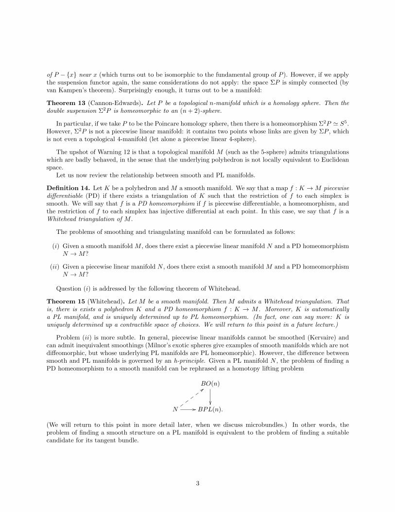
of P − x near x (which turns out to be isomorphic to the fundamental group of P ). However, if we applythe suspension functor again, the same considerations do not apply: the space ΣP is simply connected (byvan Kampen’s theorem). Surprisingly enough, it turns out to be a manifold:

Theorem 13 (Cannon-Edwards). Let P be a topological n-manifold which is a homology sphere. Then thedouble suspension Σ2P is homeomorphic to an (n+ 2)-sphere.

In particular, if we take P to be the Poincare homology sphere, then there is a homeomorphism Σ2P ' S5.However, Σ2P is not a piecewise linear manifold: it contains two points whose links are given by ΣP , whichis not even a topological 4-manifold (let alone a piecewise linear 4-sphere).

The upshot of Warning 12 is that a topological manifold M (such as the 5-sphere) admits triangulationswhich are badly behaved, in the sense that the underlying polyhedron is not locally equivalent to Euclideanspace.

Let us now review the relationship between smooth and PL manifolds.

Definition 14. Let K be a polyhedron and M a smooth manifold. We say that a map f : K →M piecewisedifferentiable (PD) if there exists a triangulation of K such that the restriction of f to each simplex issmooth. We will say that f is a PD homeomorphism if f is piecewise differentiable, a homeomorphism, andthe restriction of f to each simplex has injective differential at each point. In this case, we say that f is aWhitehead triangulation of M .

The problems of smoothing and triangulating manifold can be formulated as follows:

(i) Given a smooth manifold M , does there exist a piecewise linear manifold N and a PD homeomorphismN →M?

(ii) Given a piecewise linear manifold N , does there exist a smooth manifold M and a PD homeomorphismN →M?

Question (i) is addressed by the following theorem of Whitehead.

Theorem 15 (Whitehead). Let M be a smooth manifold. Then M admits a Whitehead triangulation. Thatis, there is exists a polyhedron K and a PD homeomorphism f : K → M . Moreover, K is automaticallya PL manifold, and is uniquely determined up to PL homeomorphism. (In fact, one can say more: K isuniquely determined up a contractible space of choices. We will return to this point in a future lecture.)

Problem (ii) is more subtle. In general, piecewise linear manifolds cannot be smoothed (Kervaire) andcan admit inequivalent smoothings (Milnor’s exotic spheres give examples of smooth manifolds which are notdiffeomorphic, but whose underlying PL manifolds are PL homeomorphic). However, the difference betweensmooth and PL manifolds is governed by an h-principle. Given a PL manifold N , the problem of finding aPD homeomorphism to a smooth manifold can be rephrased as a homotopy lifting problem

BO(n)

N //

;;

BPL(n).

(We will return to this point in more detail later, when we discuss microbundles.) In other words, theproblem of finding a smooth structure on a PL manifold is equivalent to the problem of finding a suitablecandidate for its tangent bundle.

3

Constructible Sheaves (Lecture 18)

March 7, 2011

In this lecture, we describe the theory of constructible sheaves on a polyhedron. First, we summarize afew ideas we will need from piecewise linear topology.

Definition 1. Let K be a polyhedron equipped with a triangulation T . For every simplex σ ∈ T , we definelk(σ) to be the union of those simplices τ ∈ T such that τ ∩ σ = ∅ and such that τ ∪ σ is contained in asimplex of T . The set lk(σ) is called the link of σ.

We will need the following:

Fact 2. Let M be a piecewise linear n manifold with boundary equipped with a trianguation T . If σ is a k-simplex of M which does not belong to ∂M , then lkσ(M) is PL homeomorphic to a sphere Sn−1−k ' ∂∆n−k.If σ ⊆ ∂M , then lk(σ) is PL homeomorphic to a disk Dn−1−k (with ∂ Dn−1−k being the link of σ in ∂M).

Definition 3. Let X be a polyhedron equipped with a triangulation T . We regard T as a partially orderedset (with respect to inclusions of simplices). Let C be an ∞-category. We will let ShvT (X;C) denote the ∞-category of functors from T to C. We will refer to ShvT (X;C) as the ∞-category of C-valued T -constructiblesheaves on X.

For the remainder of this lecture, we will fix a polyhedron X and a stable ∞-category C. Given atriangulation T of X, we let say that an object F ∈ ShvT (X;C) is compactly supported if F(τ) = 0 for allbut finitely many simplices τ ∈ T . Let ShvcT (X;C) denote the full subcategory of ShvT (K;C) spanned bythe compactly supported objects.

Example 4. Let τ0 ∈ T and C ∈ C, and define Fτ0,C : T → C by the formula

Fτ0,C(τ) =

C if τ0 ⊆ τ0 otherwise.

Then Fτ0,C is a compactly supported T -constructible sheaf on X. It has the following universal property:for every F ∈ ShvT (X;C), there is a canonical homotopy equivalence

MorShvT (X;C)(Fτ0,C ,F) ' MorC(C,F(τ0)).

Remark 5. The stable ∞-category ShvcT (X;C) is generated (under the formation of fibers and cofibers) byobjects of the form Fτ0,C . To prove this, let F be an arbitrary compactly supported T -constructible sheafon X; we will show that F belongs to the smallest stable subcategory of ShvcT (X;C) containing the sheavesFτ0,C . Since F is compactly supported, there exists a finite upward-closed subset T0 ⊆ T such that F(τ) = 0for τ /∈ T0. We proceed by induction on the size of T0. If T0 is empty, then F ' 0 and there is nothing toprove. Otherwise, choose a minimal element τ0 ∈ T0, let C = F(τ0), and form a cofiber sequence

Fτ0,C → F → F′ .

The desired result then follows by applying the inductive hypothesis to F′.

1

Definition 6. Let T be a trianguation of X. We define the global sections functor Γ : ShvcT (X;C) by theformula

Γ(F) = lim←−τ∈T

F(τ).

Example 7. Suppose that the polyhedron X is finite (or that C admits infinite limits). Let C ∈ C be anobject and let X0 ⊆ X be a closed subset which is of simplices belonging to T . Define FX0 by the formula

FX0(τ) =

C if τ ⊆ X0

0 otherwise.

Then Γ(FX0) can be identified with the mapping object CX0 (characterized by the universal property

MapC(C ′, CX0) = MapC(C ′, C)X0 ).Suppose now that τ is a simplex of T . The open star of τ is the union of the interiors of those simplices

which contain τ (this is an open subset of X). Let X0 be the complement of the open star of τ . We have afiber sequence of functors

Fτ,C → FX → FX0.

It follows that Γ(Fτ,C) can be identified with the mapping object C(X,X0) (which is characterized by the uni-versal property that MapC(C ′, C(X,X0)) is the homotopy fiber of the map MapC(C ′, C)X → MapC(C ′, C)X0).It is not difficult to see that X0 is a deformation retract of X − x, where x is any point belonging to theinterior of τ . We can therefore write Γ(Fτ,C) = C(X,X−x).

We now study the dependence of the ∞-category ShvT (X;C) on the choice of triangulation T . Supposethat S is a triangulation of K which refines T . Then every simplex σ ∈ S is contained in a simplex τ ∈ T .We will denote the smallest such simplex by i(σ). We regard i as a map of partially ordered sets S → T ,which induces (by composition) a functor i∗ : ShvT (X;C)→ ShvS(X;C).

Proposition 8. In the situation above, the functor i∗ is fully faithful.

Let us sketch the proof of Proposition 8. The pullback functor i∗ has a left adjoint i+ : ShvS(X;C) →ShvT (X;C), given by left Kan extension along i. Concretely, this functor can be described by the formula

(i+ F)(τ) = lim−→σ∈S,σ⊆τ

F(σ),

where F ∈ ShvS(X;C). To prove Proposition 8, we must show that for every G ∈ ShvT (X;C), the counitmap i+i

∗ G → G is an equivalence. Evaluating at a simplex τ ∈ T , we are required to prove that G(τ) isgiven by the colimit lim−→σ∈S,σ⊆τ G(i(σ)). In other words, we wish to show that the canonical map

θ : lim−→σ∈S,σ⊆τ

G(i(σ))→ lim−→σ∈S,σ⊆τ

G(τ)

is an equivalence (the right hand side is given by G(τ), since the diagram is indexed by a contractiblepartially ordered set: in fact, the geometric realization of this partially ordered set is homeomorphic to τ).Let S0 = σ ∈ S : σ ⊆ τ and let S1 = σ ∈ S : i(σ) = τ. The map θ is determined by a naturaltransformation between diagrams S0 → C, and this natural transformation is invertible when restricted toS1. To prove that θ is invertible, it suffices to show that S1 is cofinal in S0. This is a special case of thefollowing more general assertion (applied in the case M = τ):

Lemma 9. Let M be a piecewise linear n-manifold with boundary, equipped with a triangulation S. Let S1

be the collection of simplices of S which are not contained in ∂M . Then the inclusion S1 → S is cofinal.

Remark 10. Lemma 9 can be regarded as an analogue of the assertion that a manifold with boundary isalways homotopy equivalent to its interior.

2

To prove Lemma 9, we work by induction on n. Fix a simplex σ ∈ S; we wish to show that the setV1 = σ′ ∈ S1 : σ ⊆ σ′ has weakly contractible nerve. If σ ∈ S1 this is obvious (since the subset abovecontains σ as a smallest element). Let us therefore assume that σ is a simplex of the boundary ∂M . LetV = σ ∈ S : σ ( σ′. Then V can be identified with the partially ordered set of simplices of lk(σ), which(since M is a PL manifold with boundary) is PL isomorphic to a disk Dm for m < n. We can identify V0 withthe subset of V consisting of simplices which are not contained in ∂ Dm. Using the inductive hypothesis, wededuce that the inclusion V0 → V is cofinal. Since V has weakly contractible nerve, so does V0.

Proposition 8 implies that, for every F ∈ ShvT (X;C), the canonical map

Γ(F)→ Γ(i∗ F)

is an equivalence. In particular, taking F = i+ G, we obtain a canonical map

Γ(G)→ Γ(i∗i+ G) ' Γ(i+ G)

.

Proposition 11. In the above situation, the map

Γ(G)→ Γ(i+ G)

is an equivalence.

Proof. Let us assume for simplicity that G is compactly generated. Using Remark 5, we can assume thatF = Fσ,C for some simplex σ ∈ S. Then i+ F ' Fτ,C , where τ = i(σ). Choose a point x ∈ X belonging tothe interior of σ, so that x also belongs to the interior of τ . The calculation of Example 7 gives

Γ(G) ' C(X,X−x) ' Γ(i+ G).

Definition 12. Let K be a polyhedron and C an ∞-category. We let Shvconst(K;C) denote the directlimit lim←−T ShvT (X;C), where T ranges over all triangulations of X. We will refer to Shvconst(X;C) as the

∞-category of constructible C-valued sheaves on K. If C is stable, we let Shvcconst(X;C) = lim−→TShvcT (X;C);

we will refer to the objects of Shvcconst(X;C) as compactly supported constructible C-valued sheaves on X.

Construction 13. Let C be a stable ∞-category and let Q : Cop → Sp be a quadratic functor. Let K be apolyhedron with a triangulation T . We define QT : ShvcT (C)op → Sp by the formula

QT (F) = lim−→τ∈T

Q(F(τ)).

It is not difficult to see that QT is a quadratic functor on ShvcT (K,C)op, whose associative bilinear functoris given by

BT (F,F′) = lim−→τ∈T

B(F(τ),F′(τ)),

where B is the bilinear functor associated to Q.

In the situation of Construction 13, suppose we are given another triangulation S of X which refines T .Let i∗ : ShvcT (X;C)→ ShvcS(X;C) be as defined earlier. The composition

ShvcT (X;C)opi∗→ ShvcS(X;C)

QS→

is given by the formula F 7→ lim−→σ∈S Q(F(i(σ))). We claim that this composition is canonically equivalent to

QT . To prove this, it suffices to show that i induces a cofinal map Sop → T op. Unwinding the definitions, we

3

must show that for every simplex τ ∈ T , the partially ordered set σ ∈ S : i(σ) ⊆ τ has weakly contractiblenerve. This is clear, since the geometric realization of this nerve is homeomorphic to the simplex τ . Itfollows that the functors QT are compatible as T ranges over all triangulations of X, and amalgamate to aquadratic functor

Qconst : Shvcconst(X;C)op → Sp .

Let us now assume that the quadratic functor Q on C is representable, and let D be the correspondingduality functor. We claim that for every triangulation T of K, the quadratic functor QT is also representable,and the corresponding duality functor DT is given by the formula

DT (F)(τ) = lim−→σ

D(F(σ)) if τ ⊆ σ0 otherwise.

(Note that this functor carries ShvcT (K;C) to itself).For simplicity, let us assume that DT exists and show that it is given by the formula above. (A slightly

more complication version of the same argument will show that it is given by the above formula.) Fix anobject C ∈ C and a simplex τ ∈ T . For every object F ∈ ShvT (X;C), we have homotopy equivalences

MorC(C, (DT F)(τ)) ' MorShvT (X;C)(Fτ,C ,DT F)

' BT (Fτ,C ,F)

' lim−→τ ′∈T

B(Fτ,C(τ ′),F(τ ′))

' lim−→τ ′

MorC(C,

DF(τ ′) if τ ⊆ τ ′

0 otherwise.)

' MorC(C, lim−→

DF(τ ′) if τ ⊆ τ ′

0 otherwise.)

depending functorially on C, so by Yoneda’s lemma we get a canonical equivalence

(DT F)(τ) = lim−→τ ′

D(F(τ)) if τ ⊆ τ ′

0 otherwise.

Example 14. Let F be a constant functor taking the value C ∈ C.The above formula shows that

(DT F)(τ) ' DΓ(Fτ,C) = D(C(X,X−x)) = D(C) ∧ (X/X − x)

(here x ∈ X denotes a point belonging to the interior of σ, and we regard the stable∞-category C as tensoredover the ∞-category of finite pointed spaces).

4

Verdier Duality (Lecture 19)

March 9, 2011

Fix a polyhedron X and a stable ∞-category C.

Construction 1. Let Q : Cop → Sp be a quadratic functor. Let T be a triangulation of X. We defineQT : ShvcT (C)op → Sp by the formula

QT (F) = lim−→τ∈T

Q(F(τ)).

It is not difficult to see that QT is a quadratic functor on ShvcT (K,C)op, whose associative bilinear functoris given by

BT (F,F′) = lim−→τ∈T

B(F(τ),F′(τ)),

where B is the bilinear functor associated to Q.

In the situation of Construction 1, suppose we are given another triangulation S of X which refines T .Let i∗ : ShvcT (X;C)→ ShvcS(X;C) be as defined earlier. The composition

ShvcT (X;C)opi∗→ ShvcS(X;C)

QS→

is given by the formula F 7→ lim−→σ∈S Q(F(i(σ))). We claim that this composition is canonically equivalent to

QT . To prove this, it suffices to show that i induces a cofinal map Sop → T op. Unwinding the definitions, wemust show that for every simplex τ ∈ T , the partially ordered set σ ∈ S : i(σ) ⊆ τ has weakly contractiblenerve. This is clear, since the geometric realization of this nerve is homeomorphic to the simplex τ . Itfollows that the functors QT are compatible as T ranges over all triangulations of X, and amalgamate to aquadratic functor

Qconst : Shvcconst(X;C)op → Sp .

Let us now assume that the quadratic functor Q on C is representable, and let D be the correspondingduality functor. We claim that for every triangulation T of K, the quadratic functor QT is also representable,and the corresponding duality functor DT is given by the formula

DT (F)(τ) = lim−→σ

D(F(σ)) if τ ⊆ σ0 otherwise.

(Note that this functor carries ShvcT (K;C) to itself).For simplicity, let us assume that DT exists and show that it is given by the formula above. (A slightly

more complication version of the same argument will show that it is given by the above formula.) Fix an

1

object C ∈ C and a simplex τ ∈ T . For every object F ∈ ShvT (X;C), we have homotopy equivalences

MorC(C, (DT F)(τ)) ' MorShvT (X;C)(Fτ,C ,DT F)

' BT (Fτ,C ,F)

' lim−→τ ′∈T

B(Fτ,C(τ ′),F(τ ′))

' lim−→τ ′

MorC(C,

DF(τ ′) if τ ⊆ τ ′

0 otherwise.)

' MorC(C, lim−→

DF(τ ′) if τ ⊆ τ ′

0 otherwise.)

depending functorially on C, so by Yoneda’s lemma we get a canonical equivalence

(DT F)(τ) = lim−→τ ′

D(F(τ)) if τ ⊆ τ ′

0 otherwise.

Example 2. Let F be a constant functor taking the value C ∈ C.The above formula shows that

(DT F)(τ) ' DΓ(Fτ,C) = D(C(X,X−x)) = D(C) ∧ (X/X − x)

(here x ∈ X denotes a point belonging to the interior of σ, and we regard the stable∞-category C as tensoredover the ∞-category of finite pointed spaces).

Now suppose that S is a triangulation refining T . We claim that the functor

i∗ : ShvcT (X;C)→ ShvcT ′(X;C)

intertwines the duality functors DT and DT ′ . Since QT ' QT ′ i∗, for every object F ∈ ShvcT (X;C) we havea canonical map i∗DT (F) → DT ′(i∗ F). We claim that this map is invertible. To prove this, consider anarbitrary G ∈ ShvcS(X;C). We wish to prove that the canonical map

BT (i+ G,F) ' MorShvcT

(i+ G,DT F) MorShvcS(X;C)(G, i

∗DT F)→ MorShvcS(X;C)(G,DSi∗ F) ' BS(G, i∗ F)

is an equivalence. The left hand side is given by

lim−→τ∈T

B( lim−→σ∈S,σ⊆τ

G(σ),F(τ)) ' lim−→τ∈T

lim←−σ∈S,σ⊆τ

B(G(σ),F(τ)).

In the last lecture, we saw that the collection of σ ⊆ τ such that i(σ) = τ is cofinal in the collection of allσ ⊆ τ . We may therefore rewrite the above limit as

lim−→τ∈T

lim←−σ∈S,σ⊆τ

B(G(σ),F(i(σ)).

Define H : S → Spop by the formula H(σ) = B(G(σ),F(iσ)). Then the above construction is given byΓ(i+ H) (computed in the ∞-category Spop). In the last lecture, we saw that this is equivalent to

Γ(H) = lim−→σ∈S

B(G(σ),F(i(σ))) = BS(G, i∗ F),

as desired.Amalgamating the duality functors DT as T runs over all triangulations of X, we obtain a duality functor

VD : Shvcconst(X;C)op → Shvcconst(X;C).

2

We will refer to this functor as Verdier duality.Suppose now that we have two finite polyhedra X and Y , and a PL map f : X → Y . To f we can associate

a pullback functor f∗ : Shvconst(Y ;C) → Shvconst(X;C). This pullback functor admits right adjoint, whichwe will denote by f∗. For F ∈ Shvconst(X;C), can explicitly describe f∗(F) as follows. Choose triangulationsS and T of X and Y , respectively, such that F is S-constructible and f is simplicial: that is, it induces alinear map from each simplex of S to each simplex of T (carrying vertices to vertices). Then f∗ F can beidentified with the T -constructible sheaf on Y given by the formula

(f∗ F)(τ) = lim←−σ∈S,τ⊆f(σ)

F(σ).

Using a cofinality argument, we can also write

(f∗ F)(τ) = lim←−f(σ)=τ

F(σ).

Let G ∈ ShvT (Y,C). Then we have a canonical equivalence

BS(F, f∗ G) = lim−→σ

B(F(σ),G(f(σ))) = lim−→τ

lim−→f(σ)=τ

B(F(σ),G(τ)) ' lim−→τ

( lim←−f(σ)=τ

F(σ),G(τ)) = BT (f∗ F,G).

We can rewrite the left side as

MorShvS(X;C)(f∗ G,DS F) ' MorShvT (Y ;C)(G, f∗DS F)

and the right side asMorShvT (Y ;C)(G,DT f∗ F).

Yoneda’s lemma gives us a canonical isomorphism

DT f∗ F ' f∗DS F .

Passing to the direct limit over all triangulations, we deduce that Verdier duality commutes with pushfor-wards.

Proposition 3. Let Q : Cop → Sp be a nondegenerate quadratic functor. Then for any finite polyhedron Xequipped with a triangulation T , the quadratic functor QT : ShvT (X;C)op → Sp is nondegenerate. Passingto the direct limit over T , obtain a nondegenerate quadratic functor Qconst : Shvconst(X;C)op → Sp.

Proof. Let F ∈ ShvT (X;C); we wish to show that the canonical map

θF : F → DTDT F

is invertible. For every simplex τ ∈ T and every object C ∈ C, define Fτ,C by the formula

Fτ,C(τ ′) =

C if τ ′ ⊆ τ0 otherwise.

Arguing as in the previous lecture, we see that the objects Fτ,C generate the stable ∞-category ShvT (X;C).It will therefore suffice to prove that θF is an equivalence when F = Fτ,C . Note that Fτ,C = f∗ G, where fdenotes the inclusion τ → X and G is a constant functor taking the value C. Since Verdier duality commuteswith pushforwards, we can replace X by τ and thereby reduce to the case where X is a simplex, T is a thecollection of faces of X, and F is the constant functor taking the value C ∈ C. Let n be the dimension of X.

We now computeDT (F)(σ) = D(C(X,X−x))

3

where x is a point belonging to the interior of σ. If σ is a proper face of X, then X and X − x are bothcontractible so that DT (F)(σ) = 0. If σ = X, then the cofiber X/(X − x) is homotopy equivalent to Sn,so that DT (F)(σ) ' ΣnD(C). Thus DT (F) is the functor F′ given by the formula

F′(σ) =

ΣnD(C) if σ = X

0 otherwise.

We now compute DT F′ using the formula

(DT F′)(τ) = lim−→σ

DF′(σ) if τ ⊆ σ0 otherwise.

Using our formula for F′, we can rewrite this as

lim−→σ

D(ΣnD(C)) if σ = X

0 otherwise.

The nondegeneracy of Q gives an equivalence DΣnD(C) ' Σ−nC. We therefore obtain (DT F′) ' (X, ∂ X)∧Σ−nC ' C for every simplex τ ∈ T , so that we have an isomorphism DT F′ ' F. With a bit more effort,one can show that this isomorphism is given by the functor θF defined above.

4

L-Groups of Polyhedra (Lecture 20)

March 11, 2011

Let C be a stable ∞-category equipped with a nondegenerate quadratic functor Q : Cop → Sp. Let Xbe a finite polyhedron. In the last lecture, we proved that Q determines a nondegenerate quadratic functorShvconst(X;C)op → Sp. Let us denote this functor by QX , to emphasize its dependence on X. We letL(X;C, Q) denote the L-theory space of the pair (Shvconst(X;C), QX).

Example 1. When X consists of a single point, we have L(X;C, Q) ' L(C, Q).

Remark 2. Let f : X → Y be a map of finite polyhedra, and choose triangulations S and T of X and Ysuch that f is linear on each simplex. Let F ∈ ShvS(X;C). Then we have a canonical map

QS(F) ' lim−→σ∈S

Q(F(σ)) ' lim−→τ∈T

lim−→f(σ)=τ

Q(F(σ))→ lim−→τ∈T

Q( lim←−f(σ)=τ

F(σ)) = QT (f∗ F).

Taking the direct limit over triangulations, we obtain a natural transformation QX → QY f∗. This naturaltransformation induces a natural transformation

f∗ VD→ VD f∗

which we showed to be an equivalence in the previous lecture.Consequently, the pushforward functor f∗ carries quadratic objects of Shvconst(X;C) to quadratic objects

of Shvconst(Y ;C) and carries Poincare objects to Poincare objects. We obtain a map of classifying spacesPoinc(Shvconst(X;C), QX)→ Poinc(Shvconst(Y ;C), QY ). The same reasoning gives a map of simplicial spaces

Poinc(Shvconst(X;C), QX)• → Poinc(Shvconst(Y ;C), QY )•

hence a map of L-theory spacesL(X;C, Q)→ L(Y ;C, Q).

In other words, L(X;C, Q) depends functorially on X.

We now study the functor X 7→ L(X;C, Q).

Lemma 3. Let n ≥ 0 be an integer, and suppose that f, g : X → Y are homotopic PL maps of finitepolyhedra. Then f and g induce the same map Ln(X;C, Q)→ Ln(Y ;C, Q).

Proof. Replacing Q by Σ−nQ, we can reduce to the case n = 0. Let (F, q) be a Poincare object ofShvconst(X;C). We wish to show that the Poincare objects f∗ F and g∗ F are cobordant. Choose a PLmap h : X × [0, 1] → Y which is a homotopy from f to g. Let i0 : X ' X × 0 → X × [0, 1] be thecanonical map, and define i1 similarly. Since the pushforward functor h∗ carries cobordisms to cobordisms,it will suffice to show that i0,∗ F and i1,∗ F are cobordant as Poincare objects of Shvconst(X × [0, 1];C). Itnow suffices to observe that a bordism between these objects is given by p∗ F, where p : X × [0, 1] → Xdenotes the projection.

From Lemma 3 we immediately deduce the following consequence:

1

Proposition 4. Let f : X → Y be a PL homotopy equivalence between finite polyhedra. Then f induces ahomotopy equivalence L(X;C, Q)→ L(Y ;C, Q).

Let Poly denote the category whose objects are finite polyhedra and whose morphisms are PL maps. Theconstruction X 7→ L(X;C, Q) determines a functor from the category Poly to the ∞-category S of spaces.It follows from Proposition 4 that this functor factors through Poly[W−1], where Poly[W−1] denotes the∞-category obtained from Poly by formally inverting all homotopy equivalences between finite polyhedra.The ∞-category Poly[W−1] is equivalent to the full subcategory Sfin ⊆ S spanned by those spaces which arehomotopy equivalent to a finite polyhedron (or equivalently, to a finite CW complex). We may thereforeregard the functor X 7→ L(X;C, Q) as defined on the ∞-category Sfin of finite spaces.

To continue our analysis, it will be convenient to introduce a slight variation on the above construction.Let X be a finite polyhedron, and let Y ⊆ X be a closed subpolyhedron. We then have a fully faithfulembedding i∗ : Shvconst(Y ;C) → Shvconst(X;C) which commutes with Verdier duality. It follows that thequotient ∞-category Shvconst(X;C)/ Shvconst(Y ;C) inherits a nondegenerate quadratic functor. This quo-tient can be identified with a full subcategory of Shvconst(X,Y ;C) ⊆ Shvconst(X;C): namely, the subcategoryspanned by those sheaves F such that i∗ F ' 0. (Note that, for any F ∈ Shvconst(X;C), the ∞-categoryof sheaves F′ ∈ Shvconst(X;C) equipped with a map F′ → F whose cofiber is supported on Y has a finalobject, given by the extension by zero of F |(X − Y ).) We let L(X,Y ;C, Q) denote the L-theory space of(Shvconst(X,Y ;C), QX). We have seen that there is a fiber sequence of spaces

L(Y ;C, Q)→ L(X;C, Q)→ L(X,Y ;C, Q).

More generally, for Z ⊆ Y ⊆ Z, we have a fiber sequence

L(Y,Z;C, Q)→ L(X,Z;C, Q)→ L(X,Y ;C, Q).

Note that the∞-category Shvconst(X,Y ;C) can be identified with the full subcategory of Shvconst(X/Y ;C)spanned by those sheaves which vanish at the base point of X/Y . For every pointed polyhedron Z, letLred(Z;C, Q) denote the relative L-theory space L(Z, ∗;C, Q). The construction Z 7→ Lred(Z;C, Q) is func-torial with respect to pointed PL maps between pointed finite polyhedra. Moreover, Proposition 4 impliesthat it carries homotopy equivalences to homotopy equivalences, and therefore extends (in an essentiallyunique way) to a map

Lred(•;C, Q) : Sfin∗ → S,

where Sfin∗ denotes the ∞-category of pointed finite spaces.

Proposition 5. The functor Lred(•;C, Q) : Sfin∗ → S is excisive: that is, it carries homotopy pushout squares

to homotopy pullback squares.

Proof. Consider a homotopy pushout square of finite pointed spaces

X //

X ′

Y // Y ′.

Without loss of generality, we may assume that each of these spaces is a finite polyhedron, each of the mapsare PL, the horizontal maps are inclusions. Consider the diagram

Lred(X;C, Q) //

Lred(X ′;C, Q) //

Lred(X ′/X;C, Q)

θ

Lred(Y ;C, Q) // Lred(Y ′;C, Q) // Lred(Y ′/Y ;C, Q).

2

Since the rows are fiber sequences, to show that the left square is a homotopy pullback, it will suffice to showthat θ is a homotopy equivalence. This is clear, since the map X ′/X → Y ′/Y is a homotopy equivalence,by virtue of our assumption that σ is a homotopy pushout square.

It follows from Proposition 5 that we can write

Lred(X;C, Q) ' Ω∞(X ∧ L(C, Q))

for some spectrum L(C, Q), which we will call the L-theory spectrum of the pair (C, Q). In particular,L(X;C, Q) ' Lred(X+;C, Q) can be identified with the zeroth space of X+ ∧ L(C, Q). Taking X to be apoint, we get Ω∞L(C, Q) = L(C, Q), so that the homotopy groups of the spectrum L(C, Q) are the L-groupsof the pair (C, Q). More generally,

Ln(X;C, Q) ' πn(X+ ∧ L(C, Q))

is the nth homology group of X with coefficients in the spectrum L(C, Q).

3

Locally Constant Sheaves (Lecture 21)

March 21, 2011

Let X be a finite polyhedron with a triangulation T and let C be an ∞-category. We will say thatT -constructible sheaf F : T → C is locally constant if F(τ) → F(τ ′) is invertible whenever τ ≤ τ ′. Welet Shvlc(X;C) denote the full subcategory of ShvT (X;C) spanned by the locally constant sheaves. This∞-category does not depend on the choice of triangulation: if S is a refinement of T , then the pullbackfunctor ShvT (X;C) → ShvS(X;C) induces an equivalence on the full subcategories spanned by the locallyconstant sheaves.

Let R be an A∞-ring, fixed for the remainder of this lecture. Our goal is to study local systems ofR-modules on C: that is, locally constant sheaves on C with values in the ∞-category of R-modules.

Fix a finite polyhedron X and a triangulation T of X. Let ShvT (X : R) denote the ∞-category of

T -constructible sheaves on X with values in LModfpR : that is, contravariant functors T op → LModfp

R . The

formation of R-linear duals gives a contravariant equivalence of LModfpR with RModfp

R ; we may therefore

identify ShvT (X;R) with the opposite of the ∞-category coShvT (X; RModfpR ) of T -constructible cosheaves

with values in RModfpR (that is, functors T op → RModfp

R ). This is contained in the larger ∞-categorycoShvT (X; RModR) of cosheaves with values in RModR. In fact, we can identify coShvT (X; RModR) with

the ∞-category of Ind-objects Ind(coShvT (X; RModfpR ).

Let coShvlc(X : RModR) denote the full subcategory of coShvT (X; RModR) spanned by the locallyconstant cosheaves (that is, those cosheaves for which F(τ)→ F(τ ′) is an equivalence for every τ ′ ⊆ τ ∈ T ).Note that coShvlc(X; RModR) is closed under all limits and colimits in coShvT (X; RModR). It follows thatthe inclusion

coShvlc(X; RModR) → coShvT (X; RModR)

admits both left and right adjoints. We will denote a left adjoint to this inclusion by L. Let coShv0T (X; RModR)

denote the full subcategory of coShvT (X; RModR) spanned by those objects F such that T (F) ' 0: that is,

those objects F such that MorcoShvT (X;RModR)(F,G) ' 0 whenever G is locally constant. We let coShv0T (X; RModfp

R )

denote the intersection coShv0T (X; RModR) ∩ coShvT (X; RModfp

R ).

Lemma 1. The full subcategory coShv0T (X; RModR) is generated (under filtered colimits) by coShv0

T (X; RModfpR ).

Consequently, we have a canonical equivalence

coShv0T (X; RModR) ' Ind coShv0

T (X; RModfpR ).

Proof. Since every object of coShv0T (X; RModfp

R ) is a compact object of coShvT (X; RModR), we get a fullyfaithful embedding

Ind(coShv0T (X; RModfp

R )→ coShvT (X; RModR).

Let C denote the essential image of this embedding; it is a full subcategory of ShvT (X; RModR). We clearlyhave C ⊆ coShv0

T (X; RModR). Let us prove the reverse inclusion. For any object F ∈ coShv0T (X; RModR),

we can choose a fiber sequenceF′ → F

α→ F′′

1

where F′ ∈ C and Mor(G,F′′) ' 0 for every G ∈ C (here F′ is given by the colimit of the filtered diagram

of all objects of coShv0T (X; RModfp

R ) equipped with a map to F). For every simplex τ ∈ T , let Fτ ∈coShvT (X; RModR) be given by the formula

Fτ (σ) =

R if σ ⊆ τ0 otherwise.

For any cosheaf G, we have Mor(Fτ ,G) ' G(τ). Let τ ′ ⊆ τ , and form a cofiber sequence

Fτ ′ → Fτ → Fτ /Fτ ′ .

If G is locally constant, we have Mor(Fτ /Fτ ′ ,G) ' fib(G(τ)→ G(τ ′)) ' 0, so that Fτ /Fτ ′ ∈ coShv0T (X; RModfp

R ).It follows that Mor(Fτ /Fτ ′ ,F′′) ' 0, so that F′′(τ) ' F′′(τ ′). Since τ and τ ′ are arbitrary, we deduce thatF′′ is locally constant. Since F ∈ coShv0

T (X; RModR), the map α is nullhomotopic. Then F is a directsummand of F′, and therefore belongs to C as desired.

Under the contravariant equivalence of ∞-categories coShvT (X; RModfpR ) ' ShvT (X; LModfp

R ), the sub-

category coShv0T (X; RModfp

R ) corresponds to a full subcategory Shv0T (X : LModfp

R ) ⊆ ShvT (X; LModfpR ),

which is evident closed under the formation of direct summands. Several lectures ago, we constructed aquotient ∞-category

ShvT (X; LModfpR )/ Shv0

T (X; LModfpR )

as a full subcategory of Pro(ShvT (X; LModfpR )) ' Ind(coShvT (X; RModfp

R ))op ' coShvT (X; RModR)op.Unwinding the definitions, we see that this subcategory consists precisely of those objects of the form LF,where F ∈ coShvT (X; RModR)fp). Let us denote this subcategory by coShvfp

lc (X; RModR).We now study the ∞-category coShvlc(X; RModR) ' Shvlc(X; RModR) in more detail. For sim-

plicity, let us restrict our attention to the case where X is connected. For every point x ∈ X, letix : x → X denote the inclusion map. Pullback along ix determines a functor x∗ : Shvlc(X; RModR) →RModR (given by evaluation at the unique simplex τ ∈ T containing x in its interior). This functorcommutes with all limits and colimits. In particular, it admits a left adjoint, which we will denote byx+ : RModR → Shvlc(X; RModR). Since x∗ commutes with filtered colimits, x+(R) is a compact objectof Shvlc(X; RModR). Moreover, it is a compact generator of Shvlc(X; RModR): if F ∈ Shvlc(X; RModR),then Mor(x+(R),F) ' 0 if and only if MorRModR

(R, x∗ F) = x∗ F vanishes. Since X is connected, thisis equivalent to the vanishing of all stalks of F: that is, to the condition that F ' 0. It follows thatShvlc(X; RModR) is equivalent to the ∞-category RModR′ , where R′ is the A∞-ring whose underlyingspectrum is MorShvlc(X;RModR)(x+(R), x+(R)) ' MorRModR

(R, x∗x+R) ' x∗x+R.We can describe R′ more explicitly. More generally, suppose we are given any pair of points x, y ∈ X.

We can form a homotopy pullback diagram of topological spaces (commutative up to canonical homotopy)

Px,yφ //

ψ

x

x

y

y // X,

where Px,y is the path space p : [0, 1] → X : p(0) = x, p(1) = y. Let φ∗ and ψ∗ denote the pullbackfunctors on locally constant sheaves of right R-modules, and let φ+ and ψ+ be their left adjoints. There is anatural “base-change” isomorphism y∗x+ ' ψ+φ

∗ of functors from RModR to itself. Consequently, y∗x+(R)is given by ψ+ of the constant sheaf on Px,y with values in R. This is given by the smash product spectrumPx,y ∧R (here we regard Px,y as an unpointed space) whose homotopy groups are given by the R-homologygroups R∗(Px,y) of the space Px,y. In particular, we have R′ = Px,x ∧R. If R is connective, we obtain

π0R′ = R0(Px,x) =

⊕η∈π0Px,x

π0R ' (π0R)[π1X].

2

Let us now describe the full subcategory coShvfplc (X; RModR) ⊆ coShvlc(X; RModR)

θ' RModR′ . This

is a stable subcategory, consisting of those objects of the form L(F), where F ∈ coShvT (X; RModfpR ). Note

that coShvT (X; RModfpR ) is generated, as a stable ∞-category, by objects of the form Fτ,M , where

Fτ,M (σ) =

M if σ ⊆ τ0 otherwise

and M is a finitely presented right R-module. It is therefore generated as a stable ∞-category by objects ofthe form Fτ,R = Fτ . We observe that LFτ ' y+(R), where y is any point in the interior of τ : indeed, forany object G ∈ coShvlc(X; RModR) we have

Mor(LFτ ,G) ' Mor(Fτ ,G) ' G(τ) ' y∗ G ' Mor(y+(R),G).

Let x be our fixed base point of X. Since X is connected, for any point y ∈ X there is an isomorphismx+(R) ' y+(R) in coShvlc(X; RModR) (obtained by choosing a path joining x and y). Consequently, the

full subcategory coShvfplc (X; RModR) ⊆ coShvlc(X; RModR) is generated, as a stable subcategory, by the

object x+(R). In particular, it corresponds to the full subcategory

RModfpR′ ⊆ RModR

under the equivalence θ. Passing to opposite ∞-categories, we obtain the following result:

Theorem 2. Let X be a connected finite polyhedron with base point x, T a triangulation of X, R an A∞-ring, and R′ = Px,x ∧ R the A∞-ring constructed above. Let Shv0

T (X; LModfpR ) ⊆ ShvT (X; LModfp

R ) bedefined as above. Then there is a canonical equivalence of ∞-categories

ShvT (X; LModfpR )/ Shv0

T (X; LModfpR ) ' LModfp

R′ .

Let Shv0const(X; LModfp

R ) ' lim−→TShv0

T (X; LModfpR . Passing to the direct limit over T , we obtain an

equivalenceShvconst(X; LModfp

R )/ Shv0const(X; LModfp

R ) ' LModfpR′ .

Warning 3. Working with perfect module spectra in place of finitely presented module spectra, one canconstruct a fully faithful embedding

ShvT (X; LModperfR )/ Shv0

T (X; LModfpR ) ' LModperf

R′ .

This embedding is generally not an equivalence, which is why we have generally confined our attention tothe study of finitely presented modules rather than perfect modules.

Definition 4. Let X be a spectrum. We say that X is invertible if there exists another spectrum Y anda homotopy equivalence X ∧ Y ' S, where S is the sphere spectrum. One can show that a spectrum X isinvertible if and only if X ' ΣnS for some integer n. We let Spinv denote the full subcategory of Sp spannedby the invertible spectra.

Let X be a space (for now, let’s say a polyhedron). A spherical fibration over X is a locally constantsheaf on X with values in Spinv.

Example 5. Let M be a piecewise linear manifold of dimension n, and let F be the constant sheaf of spectrataking the value S. Then the Verdier dual D(F) is a spherical fibration over M . For every point x ∈ M ,we have seen that the stalk x∗D(F) can be described as the suspension spectrum of the homotopy quotientM/M − x, which is (noncanonically) homotopy equivalent to an n-sphere.

3

Now suppose that R is an A∞-ring equipped with an involution σ. Let Q : (LModfpR )op → Sp denote

either of the quadratic functors Qq or Qs. Let X be a polyhedron equipped with a triangulation T , and letζ : T → Spinv be a spherical fibration on X. We define a quadratic functor QT,ζ : ShvT (X; LModfp

R )op → Spby the formula

QT,ζ(F) = lim−→τ∈T

ζ(τ) ∧Q(F).

Since ζ is a constant functor locally onX, the work of the previous lectures shows thatQT,ζ is a nondegenerate

quadratic functor on ShvT (X; LModfpR )op. Passing to the limit over T , we obtain a nondegenerate quadratic

functorQζ : Shvconst(X; LModfp

R )op → Sp .

In particular, we obtain a “twisted” Verdier duality functor Dζ : Shvconst(X; LModfpR )op → Shvconst(X; LModfpR ),

given byDζ(F) = ζ ∧ D(F)

(where D denotes the standard Verdier duality functor discussed earlier).In the next lecture, we will apply the paradigm of Lecture 8 to the cofiber sequence of stable∞-categories

Shv0const(X; LModfp

R )→ Shvconst(X; LModfpR )→ Shvconst(X; LModfp

R )/ Shv0const(X; LModfp

R )

and the quadratic functor Qζ .

4

Assembly (Lecture 22)

March 22, 2011

Let R be an A∞-ring and let X be a connected finite polyhedron with a triangulation T . In the lastlecture, we defined a subcategory Shv0

T (X; LModfpR ) ⊆ ShvT (X; LModfp

R ). Moreover, we showed that thequotient

ShvT (X; LModfpR )/ Shv0

T (X; LModfpR

can be identified with the∞-category (RModfpR′)op ' LModfp

R′ of finitely presented R′-module spectra, whereR′ ' R ∧ Ω(X) is the A∞-ring whose modules are local systems of R-modules on X.

Our goal in this lecture is to study quadratic functors on ShvT (X; LModfpR ) which descend to the quotient

category.

Definition 1. Let X be a spectrum. We say that X is invertible if there exists another spectrum Y anda homotopy equivalence X ∧ Y ' S, where S is the sphere spectrum. One can show that a spectrum X isinvertible if and only if X ' ΣnS for some integer n. We let Spinv denote the full subcategory of Sp spannedby the invertible spectra.

Let X be a space (for now, let’s say a polyhedron). A spherical fibration over X is a locally constantsheaf on X with values in Spinv.

Example 2. Let M be a piecewise linear manifold of dimension n, and let F be the constant sheaf of spectrataking the value S. Then the Verdier dual D(F) is a spherical fibration over M . For every point x ∈ M ,we have seen that the stalk x∗D(F) can be described as the suspension spectrum of the homotopy quotientM/M − x, which is (noncanonically) homotopy equivalent to an n-sphere.

Now suppose that R is an A∞-ring equipped with an involution σ. Let Q : (LModfpR )op → Sp denote

either of the quadratic functors Qq or Qs. Let ζ : T → Spinv be a spherical fibration on X. We define aquadratic functor Qζ : ShvT (X; LModfp

R )op → Sp by the formula

Qζ(F) = lim−→τ∈T

ζ(τ) ∧Q(F).

Since ζ is a constant functor locally on X, the work of the previous lectures shows that Qζ is a nondegenerate

quadratic functor on ShvT (X; LModfpR )op. In particular, we obtain a “twisted” Verdier duality functor

Dζ : ShvT (X; LModfpR )op → ShvT (X; LModfpR ), given by

Dζ(F) = ζ ∧ D(F)

(where D denotes the standard Verdier duality functor discussed earlier).

Lemma 3. The subcategory Shv0T (X; LModfp

R ) is stable under the twisted Verdier duality functor Dζ .

Proof. For each simplex τ ∈ T , define Fτ ∈ ShvT (X; LModfpR ) by the formula

Fτ (σ) =

R if σ ⊆ τ0 otherwise.

1

Whenever τ ′ ⊆ τ , we have a canonical map Fτ → Fτ ′ . Let us denote the fiber of this map by Fτ,τ ′ . We saw

in the previous lecture that Shv0T (X; LModfp

R ) is generated by the objects Fτ,τ ′ . It will therefore suffice to

show that each Dζ Fτ,τ ′ belongs to Shv0T (X; LModfp

R ).If τ ′ ⊂ τ ′′ ⊂ τ , then we have a fiber sequence

Fτ,τ ′′ → Fτ,τ ′ → Fτ ′′,τ ′ .

We may therefore reduce to proving the lemma for the pairs (τ, τ ′′) and (τ ′′, τ ′). Suppose that τ ' ∆n

and that τ ′ is a face of τ ; let K denote the closure of ∂ τ − τ ′. Since τ is contractible, ζ is constant on τ ;it will therefore suffice to show that DFτ,τ ′ belongs to Shv0

T (X; LModfpR ). A simple calculation shows that

Σ−nDFτ,τ ′ is given by the formula

σ 7→

R if σ ⊆ τ, σ * K

0 otherwise.

We can choose a different triangulation of X for which τ and K are simplices of the triangulation, in whichcase the sheaf abvoe is given by Fτ,K , and therefore belongs to Shv0

const(T ; LModfpR ).

Using the formalism of Lecture 8, we see that Qζ descends to give a quadratic functor Qlc on LModfpR′ .

When Q = Qs, we will denote this functor by Qslc; when Q = Qq, we will denote this functor by Qqlc. Using thefact that Qq and Qs have the same associated bilinear functor B, we deduce that Qslc and Qqlc have the sameassociated bilinear functor Blc. Let us try to describe this bilinear functor more explicitly. Set Q = Qs, sothat R is a Poincare object of LModfp

R . Let x ∈ X be our chosen base point. We will assume that x is a vertexof the triangulation T , and suppose that the invertible spectrum ζx is homotopy equivalent to the spherespectrum (something that can always be achieved by an appropriate shift). Let x∗(R) ∈ ShvT (X; LModfp

R )denote the skyscraper sheaf with stalk R at the point x (and vanishing elsewhere). Then x∗(R) has the

structure of a Poincare object of ShvT (X; LModfpR ). It follows that the image of x∗(R) in the ∞-category

LModfpR′ has the structure of a Poincare object of LModfp

R′ . By construction, this image can be identifiedwith R′ itself. Arguing as in Lecture 10, we deduce that R′ is equipped with an involution σ, and that thebilinear functor Blc : (LModfp

R )op × (LModfpR )op → Sp is given by (M,N) 7→ MorR′−R′(M ∧N,R′).

Remark 4. To be even more explicit, one would like to describe the involution on the A∞-ring R′. Thisinvolves a mixture of three ingredients:

(i) The given involution on R.

(ii) The involution of the loop space Ω(X) ' Px,x, given by reading each path in the opposite direction.

(iii) The nontriviality of the spherical fibration ζ

Suppose for example that R is connective, so that R′ is connective and we have a canonical isomorphism ofassociative rings π0R

′ ' (π0R)[π1X]. Then the involution on π0R′ is given by∑

g∈π1X

λgg 7→∑

g∈π1X

ε(g)σ(λg)g−1

where σ denotes the underlying involution on π0R and ε : π1X → ±1 is the obstruction to choosing anorientation of the spherical fibration ζ.

Now armed with our description of Blc, let us try to to describe Qlc in the special case where Q = Qq.Let us regard Q as a covariant functor RModfp

R → Sp, given by Q(M) = B(M,M)hΣ2. Then Qζ corresponds

to the covariant functor coShvT (X; RModfpR )→ Sp given by

Qζ(F) = lim−→τ∈T

ζ(τ) ∧B(F(τ),F(τ))hΣ2 .

2

We can extend this to a functor

Qζ(F) : Ind(coShvT (X; RModfpR )) ' coShvT (X; RModR)→ Sp

which commutes with filtered colimits; this is again given by the formula

Qζ(F) = lim−→τ

ζ(τ) ∧ (F(τ) ∧R F(τ))hΣ2

The quadratic functorQlc : (LModfp

R′)op ' RModfp

R′ → Sp

is given by composing Qζ with the fully faithful embedding

θ : RModfpR′ ⊆ RModR′ ' coShvlc(X : RModR) ⊆ coShvT (X; RModR).

It follows that the polarization Blc is given by composing θ with the map Bζ , given by

(F,G) 7→ lim−→τ

ζ(τ) ∧ (F(τ) ∧R G(τ)).

We deduce that the natural map Blc(M,M)hΣ2 → Qqlc is an equivalence. This proves the following:

Proposition 5. Let R be an A∞-ring with involution, let X be a connected finite polyhedron with base pointx, let ζ be a spherical fibration over X equipped with a trivialization at x, and let R′ ' R∧Ω(X) be defined as

above. Then the L-theory spectrum L(Shvconst(X; LModfpR )/ Shv0

const(X; LModfpR ), Qqlc) can be identified with

the quadratic L-theory spectrum Lq(R′) of the A∞-ring R′, equipped with the involution described above. In

particular, if R is connective, there is a canonical equivalence L(Shvconst(X; LModfpR )/ Shv0

const(X; LModfpR ), Qqlc) '

Lq((π0R)[π1X]), where the involution on the group ring (π0R)[π1X] is described in Remark 4.

The analogous statement is generally not true for symmetric L-theory, because the construction M 7→(M ∧RM)hΣ2 generally does not commute with filtered colimits. This motivates the following definition:

Definition 6. Let R be an A∞-ring with involution, let X be a finite polyhedron, and let ζ be a spherical fi-bration onX. We let Lv(X,ζ)(R) denote the L-theory spectrum associated to (Shvconst(X; LModfp

R )/Shv0const(X; LModfp

R ), Qslc).

We will refer to L(X,ζ)v(R) as the visible L-theory spectrum of X.

Assume that X is connected with base point x. We then have a commutative diagram

L(Shvconst(X; LModfpR ), Qqζ)

//

L(Shvconst(X; LModfpR ), Qsζ)

Lq(R′) // Lv(X,ζ)(R).

If we assume that ζ is trivial and that R is connective, this simplifies to a commutative diagram of spectra

X ∧ Lq(R) //

X ∧ Ls(R)

Lq((π0R)[π1X]) // Lv(X,ζ)(R).

The vertical maps here are referred to as assembly maps.

Proposition 7. The diagrams above are homotopy pullback squares.

3

Proof. It suffices to show that we get a homotopy equivalence between the homotopy fibers of the verticalmaps. Using localization theorem of Lecture 8, we can identify these homotopy fibers with the L-theoryspectra of Shv0

const(X; LModfpR ) with respect to Qqζ and Qsζ , respectively. It will therefore suffice to show that

the canonical map Qqζ → Qsζ is an equivalence when evaluated on any F ∈ Shv0const(X; LModfp

R ).

Let U : (LModfpR )op → Sp be the homotopy cofiber of the map Qq → Qs, so that U is given by the

formula U(M) = MorR−R(M ∧M,R)tΣ2 . Then U is an exact functor. It follows that U(R) has the structureof an R-module spectrum, and that U is given by the formula U(M) = MorR(M,U(R)). We deduce that

for F ∈ ShvT (X; LModfpR ), the cofiber of the map Qqζ(F)→ Qsζ(F) is given by

lim−→τ∈T

ζ(τ) ∧ U(F(τ)) = MorR(lim←−τ

ζ(τ)−1 ∧ F(τ), U(R)).

If F ∈ Shv0const(X; LModfp

R ), then the limit lim←−τ ζ(τ)−1 ∧ F(τ) vanishes (since it is the spectrum of maps

from the locally constant sheaf ζ ∧R into F).

4

Orientations of L-Theory (Lecture 23)

March 24, 2011

In the last lecture, we introduced the L-theory spectra Lq(X, ζ,R) and Ls(X, ζ,R), where R is an A∞-ring with involution, X is a finite polyhedron, and ζ is a spherical fibration on X. When ζ is trivial, thesespectra are given simply by X ∧Lq(R) and X ∧Ls(R), respectively. In general, they depend on the sphericalfibration ζ. However, our excision argument generalizes to show that Lq(X, ζ,R) is given by the homotopycolimit

lim−→τ∈T

L(LModfpR , ζ(τ) ∧Qq)

where T denotes any triangulation of X. In other words, the homotopy groups of Lq(X, ζ,R) are given by

the homology of X with coefficients in a local system of spectra, given by (x ∈ X) 7→ L(LModfpR , ζ(x)∧Qq).

This raises the following general question:

Question 1. Let C be a stable ∞-category equipped with a nondegenerate functor Q, and let E be aninvertible spectrum. What is the relationship between the L-theory spectra L(C, Q) and L(C, E ∧Q)?

In the situation of Question 1, we can write E ' S−n for some integer n. We have seen that there is acanonical isomorphism Lk(C,ΩnQ) = Lk+n(C, Q), suggesting that we should have an equivalence of L-theoryspectra L(C,ΩnQ) ' ΩnL(C, Q). In other words, we have a homotopy equivalence

θE : L(C, E ∧Q) ' E ∧ L(C, Q).

For our purposes, we need to know this not just for an individual invertible spectrum E, but in the casewhere E ranges over the fibers of some spherical fibration. It is therefore important that our analysis befunctorial with respect to automorphisms of E. In fact, it is not possible to choose θE to be functorial withrespect to all automorphisms of E. However, we will show that it can be chosen to depend naturally onautomorphisms which are of geometric origin.

Definition 2. Let M be PL manifold, and let S denote the local system of spectra on M taking the constantvalue S (where S is the sphere spectrum). The Verdier dual D(S) is a spherical fibration over M . We willdenote the inverse of this spherical fibration by ζM . We refer to ζM as the normal spherical fibration of M .Unwinding the definitions, it can be described by the formula

ζM (x) = (Σ∞(M/M − x))−1.

There is a canonical map of spectra S → Γ(M ;S). If M is compact, this dualizes to give a map

Γ(M ;DS) ' DΓ(M ;S)→ S.

This map gives a point in the zeroth space of the spectrum

MorSp(lim←−τ∈T

(DS)(τ), S) ' lim−→τ∈T

ζM (τ)

where T denotes some triangulation of M . We will denote this point by [M ] and refer to it as the fundamentalclass of M .

1

More generally, if M is a PL manifold with boundary, we let ζM denote the local system of spectra onM obtained by extending the normal spherical fibration from the interior of M (note that the interior ofM is homotopy equivalent to M , so there exists an essentially unique extension). In this case, we have afundamental class

[M ] ∈ Ω∞(lim−→τ∈T

ζM (τ) if τ * ∂M

0 otherwise.

Let us now fix a PL manifold with boundary M . Let C be a stable ∞-category equipped with a nonde-generate quadratic functor Q. For each triangulation T of M , let

QζM ,T : ShvT (M,∂M ;C)op → Sp

be given by the formula

lim−→τ

QζM ,T (F(τ)) ∧ ζM (τ) if τ * ∂M

0 otherwise.

Let C ∈ C be an object, and let C denote the constant sheaf on M with taking the value C (which we willidentify with its image in ShvT (M,∂M ;C)). We then obtain a homotopy equivalence

QζM ,T (C) ' Q(C) ∧ lim−→τ∈T

ζM (τ) if τ * ∂M

0 otherwise.

In particular, the fundamental class [M ] determines a map

Q(C)→ QζM ,T (C),

which we will denote by q 7→ q[M ]. This constuction carries Poincare objects to Poincare objects, and inducesa map of L-theory spectra

Φ : L(C, Q)→ L(Shvconst(M,∂M ;C);QζM )

(where QζM denotes the amalgamation of the quadratic functors QζM ,T where T ranges over all triangulationsof M).

Example 3. Let M be a piecewise linear disk. For every point x in the interior of M , we have a canonicalhomotopy equivalence of pairs (M,∂M)→ (M,M −x). Consequently, ζM is canonically equivalent to theconstant sheaf taking the value E, where E−1 = Σ∞(M/∂M). It follows that L(Shvconst(M,∂M ;C), Qζ) isgiven by (M,∂M) ∧ L(C, E ∧Q) ' E−1 ∧ L(C, E ∧Q). We may therefore identify Φ with a map of spectraE ∧ L(C, Q)→ L(C, E ∧Q).

Suppose M ' ∆n. Then Φ determines maps Lk+n(C, Q)→ Lk(C,ΩnQ), which can be identified with theshift isomorphisms defined earlier. It follows that Φ is a homotopy equivalence whenever M is a piecewiselinear disk.

The construction of Φ is functorial with respect to piecewise linear homeomorphisms of the PL manifoldM .

Let us now introduce some terminology to describe the situation more systematically.Let X be a polyhedron. A closed n-disk bundle over X is a map of polyhedra q : D → X such that every

point x ∈ X has an open neighborhood U for which there is a PL homeomorphism q−1U ' U ×∆n (whichcommutes with the projection to U).

There is a canonical bijection between isomorphism classes of closed n-disk bundles over X and homotopyclasses of maps X → BDisk(n), where BDisk(n) denotes the classifying space of the (simplicial) groupDisk(n) of PL homeomorphisms of ∆n.

The disjoint union∐nBDisk(n) is equipped with a multiplication which is associative up to coherent ho-

motopy, classifying the formation of products of closed n-disk bundles. We can describe the group completionof

∐nBDisk(n) as a product Z× BPL, where BPL is the direct limit lim−→n

BDisk(n).

2

Let Pic(S) denote the classifying space for invertible spectra (so that homotopy classes of maps X →Pic(S) correspond to equivalence classes of spherical fibrations over X). Every closed disk bundle q : D → Xhas an associated spherical fibration, given by x 7→ Σ∞(Dx/ ∂ Dx). This construction determines a map∐nBDisk(n) → Pic(S), which is multiplicative up to coherent homotopy and therefore extends to a map

Z× BPL→ Pic(S).Fix (C, Q) as above. Over the space Pic(S), we have two local systems of spectra: one given by the

formula E 7→ L(C, E ∧Q) and one given by the formula E 7→ E ∧ L(C, Q). The above analysis implies thatthese two local systems are canonically equivalent when restricted to Z× BPL. This proves the following:

Proposition 4. Let X be a finite polyhedron with triangulation T , C a stable ∞-category equipped witha nondegenerate quadratic functor Q, and ζ a spherical fibration on X, classified by a map X → Pic(S).Suppose that this classifying map factors through Z×BPL (that is, that the spherical fibration ζ arises froma closed disk bundle, at least stably). Then there is a homotopy equivalence (depending canonically on thefactorization)

L(Shvconst(X;C), Qζ) ' lim−→τ∈T

ζ(τ) ∧ L(C, Q).

We can also make the analysis of the preceding discussion read in a different way. Let us suppose thatC = Dfp(Z) is the ∞-category of perfect complexes of Z-modules, and let Q be either Qq or Qs. Then Qis a spectrum valued functor which factors through the ∞-category of Z-module spectra. It follows that forevery spectrum E, we can write E ∧ Q ' (E ∧ Z) ∧Z Q, so that E ∧ Q depends only on the generalizedEilenberg-MacLane spectrum E ∧ Z. Let ζ be a spherical fibration on a polyhedron X, and suppose that ζassigns to each point x ∈ X a spectrum ζ(x) which is homotopy equivalent to ΣnS. Suppose further that ζ isorientable. A choice of orientation determines a canonical homotopy equivalence of each ζ(x)∧Z with ΣnZ,and therefore a natural isomorphism Qζ ' ΣnQ. It follows that we obtain a canonical homotopy equivalence

lim−→τ∈T

ζ(τ)∧L(C, Q) ' L(Shvconst(X;C), Qζ) ' L(Shvconst(X;C),ΣnQ) ' ΣnL(Shvconst(X;C), Q) ' Σn(X∧L(C, Q)).

This proves:

Proposition 5. If ζ is an oriented spherical fibration (of dimension n) on X classified by a map X → Pic(S)which factors through Z × BPL, then we have homotopy equivalences (depending canonically on the choiceof factorization)

lim−→τ∈T

ζ(τ) ∧ Lq(Z) ' Σn(X ∧ Lq(Z))

lim−→τ∈T

ζ(τ) ∧ Ls(Z) ' Σn(X ∧ Ls(Z))

Remark 6. Proposition 5 can be interpreted as saying that every orientable PL bundle is oriented withrespect to the ring spectrum Ls. We will return to this point in the next lecture.

3

L-Theory Orientations of Manifolds (Lecture 24)

March 30, 2011

Let us begin by introducing some terminology to systematize the ideas of the previous lecture. Let X bea polyhedron. A closed n-disk bundle over X is a map of polyhedra q : D → X such that every point x ∈ Xhas an open neighborhood U for which there is a PL homeomorphism q−1U ' U × ∆n (which commuteswith the projection to U).

There is a canonical bijection between isomorphism classes of closed n-disk bundles over X and homotopyclasses of maps X → BDisk(n), where BDisk(n) denotes the classifying space of the (simplicial) groupDisk(n) of PL homeomorphisms of ∆n.

The disjoint union∐nBDisk(n) is equipped with a multiplication which is associative up to coherent ho-

motopy, classifying the formation of products of closed n-disk bundles. We can describe the group completionof

∐nBDisk(n) as a product Z× BPL, where BPL is the direct limit lim−→n

BDisk(n).

Let Pic(S) denote the classifying space for invertible spectra (so that homotopy classes of maps X →Pic(S) correspond to equivalence classes of spherical fibrations over X). Every closed disk bundle q : D → Xhas an associated spherical fibration, given by x 7→ Σ∞(Dx/ ∂ Dx). This construction determines a map∐nBDisk(n) → Pic(S), which is multiplicative up to coherent homotopy and therefore extends to a map

Z× BPL→ Pic(S).Fix (C, Q) as above. Over the space Pic(S), we have two local systems of spectra: one given by the

formula E 7→ L(C, E ∧Q) and one given by the formula E 7→ E ∧L(C, Q). The constructions of the previouslecture show that these spherical fibrations are (canonically) equivalent when restricted to Z× BPL.:

Proposition 1. Let X be a finite polyhedron with triangulation T , C a stable ∞-category equipped witha nondegenerate quadratic functor Q, and ζ a spherical fibration on X, classified by a map X → Pic(S).Suppose that this classifying map factors through Z×BPL (that is, that the spherical fibration ζ arises froma closed disk bundle, at least stably). Then there is a homotopy equivalence (depending canonically on thefactorization)

L(Shvconst(X;C), Qζ) ' lim−→τ∈T

ζ(τ) ∧ L(C, Q).

Now suppose that M is a compact PL manifold with boundary and let ζM be its normal fibration. ThenζM factors canonically through Z × BPL. Let T be a triangulation of M , so that we have a canonicalorientation

[M ] : S → lim−→τ∈T

0 if τ ⊆ ∂MζM (τ) otherwise.

Smashing with L(C, Q) and using Proposition 1, we obtain a map

L(C, Q) → lim−→τ∈T

0 if τ ⊆ ∂MζM (τ) ∧ L(C, Q)

' lim−→τ∈T

0 if τ ⊆ ∂ML(C, ζM (τ) ∧Q)

' L(Shvconst(M,∂M ;C), QζM ).

1

This can be identified with the map constructed in the previous lecture, which carries each Poincare object(C, q) to a Poincare object (C, q[M ]), where C denotes the constant sheaf taking the value C.

We can also make the analysis of the preceding discussion read in a different way. Let us suppose thatC = Dfp(Z) is the ∞-category of perfect complexes of Z-modules, and let Q be either Qq or Qs. Then Qis a spectrum valued functor which factors through the ∞-category of Z-module spectra. It follows that forevery spectrum E, we can write E ∧ Q ' (E ∧ Z) ∧Z Q, so that E ∧ Q depends only on the generalizedEilenberg-MacLane spectrum E ∧ Z. Let ζ be a spherical fibration on a polyhedron X, and suppose that ζassigns to each point x ∈ X a spectrum ζ(x) which is homotopy equivalent to ΣnS. Suppose further that ζ isorientable. A choice of orientation determines a canonical homotopy equivalence of each ζ(x)∧Z with ΣnZ,and therefore a natural isomorphism Qζ ' ΣnQ. It follows that we obtain a canonical homotopy equivalence

lim−→τ∈T

ζ(τ)∧L(C, Q) ' L(Shvconst(X;C), Qζ) ' L(Shvconst(X;C),ΣnQ) ' ΣnL(Shvconst(X;C), Q) ' Σn(X∧L(C, Q)).

This proves:

Proposition 2. If ζ is an oriented spherical fibration (of dimension n) on X classified by a map X → Pic(S)which factors through Z × BPL, then we have homotopy equivalences (depending canonically on the choiceof factorization)

lim−→τ∈T

ζ(τ) ∧ Lq(Z) ' Σn(X ∧ Lq(Z))

lim−→τ∈T

ζ(τ) ∧ Ls(Z) ' Σn(X ∧ Ls(Z))

Let L denote the symmetric L-theory spectrum Ls(Z). Tensor product of chain complexes endows Lwith the structure of a ring spectrum (in fact, an E∞-ring spectrum). Let X be a space and let ζ be anoriented spherical fibration (of dimension n) over X whose classifying map factors through Z × BPL. Theabove argument shows that the local system

(x ∈ X) 7→ Σ−n(ζ(x) ∧ L)

is equivalent to the constant local system taking the value L. In particular, this local system has a canonicalglobal section; let us denote it by α.

Let us identify the field Q of rational numbers with the corresponding Eilenberg-MacLane spectrum.Since ζ is oriented, the local system

(x ∈ X) 7→ Σ−n(ζ(x) ∧Q)

is (canonically) equivalent to the constant local system taking the value Q. Let LQ = LQ denote therationalization of L. Smashing with L, we obtain a trivialization of the local system

(x ∈ X) 7→ Σ−n(ζ(x) ∧ LQ).

Under this equivalence, α determines a section of the constant local system taking the value LQ. That is,we can identify α with an (invertible) element l(ζ) in the cohomology ring (LQ)0(X). This element dependsnaturally on the pair (X, ζ) (together with the orientation and PL-structure on ζ). We may thereforeregard l(ζ) as a characteristic class of oriented PL bundles ζ. It measures the discrepancy between two LQ-orientations of ζ: one coming from the L-orientation defined above, and the other from the Q-orientaitonon ζ.

Using our calculation of the homotopy groups of Lq(Z), we can be more explicit. We have seen thatthere is an isomorphism of commutative rings π∗L ' Q[t±1], where t lies in degree −4. We therefore have ahomotopy equivalence of spectra LQ '

∏k∈Z Σ−4kQ, and therefore an isomorphism of graded rings

(LQ)∗(X) '∏k∈Z

H∗+4k(X;Q) ' H∗(X;Q)[[t]]

2

In particular, we can identify (LQ)0(X) with the ring∏k≥0 H4k(X;Q), so that l(ζ) can be written as a

formal suml0(ζ) + l1(ζ) + · · ·

where lk(ζ) ∈ H4k(X; ζ).Now suppose that M is a compact closed oriented PL manifold of dimension n. Then M has orientations

with respect to both Q and the L-theory spectrum L, giving us fundamental classes

[M ]Q ∈ Hn(X;Q) [M ]L ∈ Ln(M).

Let us identify [M ]Q and [M ]L with their images in (LQ)n(M). We then have

[M ]Q = l(ζ)[M ]L

where ζ denotes the normal fibration of M . The projection map p : M → ∗ induces a pushforward

p∗ : (LQ)n(M)→ (LQ)n(∗) =

Q if n = 4k

0 otherwise.

By construction, [M ]L is represented by the constant sheaf on M taking the value Z, regarded as a Poincareobject of Shvconst(M), so that p∗([M ]L) can be represented by the cochain complex C∗(M ;Z), regarded as

a Poincare object of LModfpZ . If n = 4k, then the isomorphism (LQ)n ' Q carries p∗(M) to the signature

σM of the manifold M . This proves an abstract version of the Hirzebruch signature formula: we have

σM = p∗([M ]L) ' p∗(l(ζ)[M ]Q) = l(ζ)k[M ],

where l(ζ)k denotes the kth term in the characteristic class l(ζ) described above.

3

The Hirzebruch Signature Formula (Lecture 25)

March 30, 2011

In the last lecture, we defined a characteristic class l(ζ) ∈∏k H4k(X;Q) associated to an oriented PL

bundle on a space X, given byl(ζ) = l0(ζ) + l4(ζ) + · · ·

If M is a compact oriented PL manifold of dimension 4k and ζ is its (stable) normal bundle, then thesignature of M is given by

σM = l4k(ζ)[M ].

To obtain the Hirzebruch signature formula, we need to describe the characteristic class l(ζ) explicitly. Forsimplicity, let us restrict our attention to the case where ζ comes from a (virtual) vector bundle of rank zero,

so that ζ is classified by a map Xχ→ BSO = lim−→BSO(n). Then ζ is the pullback of a universal bundle ζ0 on

BSO, so that l(ζ) = χ∗l(ζ0). It will therefore suffice to describe l(ζ0) as an element of the cohomology ring∏k H4k(BSO;Q) ' Q[[p1, p2, . . .]]; here pi denote the universal Pontryagin classes.

Remark 1. Our restriction to virtual vector bundles of rank zero involves no essential loss of generality.First, the characteristic class l(ζ) does not change if we add a trivial bundle to ζ, so we may as well assumethat ζ is of degree zero and classified by a map X → BSPL (where SPL denotes the index two subgroup ofPL corresponding to homeomorphisms which preserve orientation). At the very end of this course, we willsee that the map BSO→ BSPL is a rational homotopy equivalence.

Every complex vector bundle can be regarded as an oriented real vector bundle. This observation deter-mines a map of classifying spaces BU→ BSO. The induced map

H∗(BSO;Q)→ H∗(BU;Q)

is injective on cohomology. Consequently, to describe l(ζ0), it will suffice to describe its image in H∗(BU(n);Q)for every integer n. According to the splitting principle for complex line vector bundles, the canonical map

H∗(BU(n);Q)→ H∗(BU(1)n;Q) ' H∗(BU(1);Q)⊗n

is injective on cohomology. In other words, it suffices to describe l(ζ) in the special case where ζ comes froma complex vector bundle of rank n that is written as a direct sum ζ1⊕ · · · ⊕ ζn of complex line bundles. Ourconstruction of L-theory orientations is compatible with the formation of direct sums of PL disk bundles, sowe have

l(ζ) =∏

1≤i≤n

l(ζi).

We are therefore reduced to describing l(ζ) when ζ arises from a complex line bundle. Here it suffices totreat the case X = BU(1) = CP∞, so that H∗(X;Q) ' Q[[H]] where H ∈ H2(X;Q) denotes the first Chernclass of the universal line bundle. We can therefore write l(ζ) = f(H) for some power series f with rationalcoefficients, which are yet to be determined. Note that since f(H) lies in

∏k H4k(X;Q), the power series f

is even: that is, we have f(H) = f(−H), so that f can be written as a function of H2.

1

We can determine the power series f by applying the signature formula to the manifolds CPn, where nranges over the integers. Note that the tangent bundle T to CPn fits into an exact sequence

0→ O→ O(1)n+1 → T → 0.

If we let ζCPn denote the normal bundle to CPn, we have l(ζCPn) = l(T )−1 = l(O(1))−n−1 = f(H)−n−1.The fundamental class of CPn is dual to Hn. It follows that the signature σ(CPn) of CPn is given by thecoefficient of Hn in the power series f(H)−n−1. Equivalently, the signature of CPn is given by the residueof (formal) differential ( 1

Hf(H) )n+1dH.

We can describe this residue more explicitly using the Lagrange inversion formula. Since the constantterm of f is invertible, Hf(H) is an invertible power series. That is, if we set U = Hf(H), then there is apower series g such H = g(U) =

∑ciU

i. Then ( 1Hf(H) )

n+1dH = 1Un+1 dg(U) = 1

Un+1 g′(U)dU . The residue

of this formal series is given by (n+ 1)cn+1. It follows that

g(U) ==∑ σ(CPn)

n+ 1Un+1 = U +

U3

3+U5

5+ · · · .

This power series describes the transcendental function tanh−1, so that Hf(H) = tanh(H) and f(H) =tanh(H)

H .Let us now make the above formula more explicit. When ζ comes from a complex line bundle, it has a

first Chern class c1(ζ), and l(ζ) is given by f(c1(ζ)). Since f is really a function of H2, we can write f(c1(ζ))as a power series in the Pontryagin class p1(ζ) = c1(ζ)2. Informally, we have

l(ζ) =tanh(

√p1(ζ))√

p1(ζ)

If ζ is a sum of complex line bundles ζ1, ζ2, . . . , ζn, then we have

l(ζ) =∏i

l(ζi) =∏i

tanh(√p1(ζi))√

(p1(ζi).

This can be written as an (infinite) sum of symmetric polynomials in the variables p1(ζ1), . . . , p1(ζn). Itcan therefore be rewritten as an (infinite) sum of polynomials in the elementary symmetric polynomials inthe variables p1(ζ1), . . . , p1(ζn), which are the Pontryagin classes p1(ζ), p2(ζ), . . . , pn(ζ). Taking the limit asn→∞, we obtain a formula for l(ζ) in terms of the Pontryagin classes of ζ (which is valid for any orientablereal vector bundle, by virtue of the above remarks concerning injectivity on cohomology).

We can recast the above discussion in the language of complex oriented cohomology theories. Thesymmetric L-theory spectrum Ls(Z) is orientable with respect to all oriented real vector bundles, and inparticular has a canonical complex orientation. Following Quillen, we can associate to Ls(Z) a formal grouplaw. The above calculation can be interpreted as saying that (modulo torsion) this formal group law is givenby

(X,Y ) 7→ tanh(tanh−1(X) + tanh−1(Y )).

That is, tanh is the inverse of the logarithm for the formal group law determined by our complex orientationon Ls. Let

p(X) = X +X2

2+X3

6+ · · · = eX − 1

be the inverse of the logarithm for the multiplicative formal group law. Then

tanh(X) =eX − e−X

eX + e−X=e2X − 1

e2X + 1=

p(2X)

p(2X) + 2.

2

After inverting 2, we see that tanh(X) and p(X) differ by an invertible change of coordinate. It follows thatthe formal group law

(X,Y ) 7→ tanh(tanh−1(X) + tanh−1(Y ))

is isomorphic to the multiplicative formal group after inverting 2. Using Landweber exactness, we seethat the spectrum Ls(Z)[ 12 ] ' Lq(Z)[ 12 ] is determined up to homotopy equivalence by the graded ringπ∗Ls(Z)[ 12 ] ' Z[ 12 ][t±1] together with the associated formal group, which is the multiplicative group. Thisyields a proof of the following result:

Proposition 2. There is a homotopy equivalence of spectra Ls(Z)[ 12 ] ' KO[ 12 ], where KO denotes the realK-theory spectrum.

3

Poincare Spaces and Spivak Fibrations (Lecture 26)

April 1, 2011

Let X be a topological space and C an ∞-category. We let Shvlc(X;C) denote the ∞-category of mapsfrom the Kan complex Sing•(X) into C. We will refer to Shvlc(X;C) as the ∞-category of locally constantC-valued sheaves on X, or sometimes as the ∞-category of local systems of C-valued sheaves on X. If X is apolyhedron with triangulation T , then we can identify Shvlc(X;C) with the full subcategory of ShvT (X;C)spanned by those functors which carry each inclusion τ ⊆ τ ′ of simplices to an invertible morphism of C.

Let f : X → Y be a map of topological spaces. Then f induces a pullback functor f∗ : Shvlc(Y ;C) →Shvlc(X;C). Suppose that C is the ∞-category of spectra. Then f∗ preserves all limits and colimits, andtherefore admits both a left adjoint f! and a right adjoint f∗.

In the special case where Y is a point, we will denote the functors f! and f∗ by C∗(X; •) and C∗(X; •),respectively. If X si a polyhedron with triangulation T , these are described by the formulas

C∗(X;F) = lim−→τ

F(τ) C∗(X;F) = lim←−τ

F(τ).

If X is a finite polyhedron, we conclude that the construction C∗ : Shvlc(X; Sp) → Sp commutes withhomotopy colimits.

Suppose now that X is connected with base point x. Then Shvlc(X; Sp) can be identified with the∞-category of modules over the A∞-ring R = Σ∞+ Ω(X). Any functor F : LModR → Sp is determined byits value F (R) ∈ Sp, together with its right R-module structure. Indeed, the fact that F commutes withhomotopy colimits implies that F is given by F (M) ' F (R)∧RM . We can identify F (R) with a local systemζ on X, so that F is given by the formula F (M) = C∗(X;M ∧ ζ). This description generalizes immediatelyto the case where X is not assumed to be connected:

Proposition 1. Let F : Shvlc(X; Sp)→ Sp be a functor which commutes with homotopy colimits. Then Fis given by F (F) = C∗(F∧ζ), where ζ is a local system of spectra on X. Moreover, the local system ζ isdetermined uniquely up to equivalence.

In particular, if X is a finite polyhedron (or any space equivalent to a finite polyhedron) and f : X → ∗denotes the projection map, we have an equivalence of functors

f∗(•) ' C∗(• ∧ ζX)

for some local system ζX on X.

Definition 2. We say that a finite polyhedron X is a Poincare space if ζX is a spherical fibration (thatis, if each of the fibers ζX(x) is an invertible spectrum). In this case, we say that ζX is the Spivak normalfibration of X.

Remark 3. Let X be a finite polyhedron containing a point x. Let i : x → X denote the inclusion andp : X → ∗ the projection map, so that p i is a homeomorphism. Then we have a homotopy equivalence ofspectra

i∗ζX ' (p i)!i∗ζX ' p!(i!i

∗ζX) ' p!((i!S) ∧ ζX) ' C∗(X; i!S).

1

In other words, the stalk ζX(x) is given by taking global sections of the local system of spectra on X thatassigns to each point y ∈ X the suspension spectra Σ∞+ Px,y, where Px,y denotes the path space p : [0, 1]→X : p(0) = x, p(1) = y.

Remark 4. Let S denote the constant local system on X with value the sphere spectrum, so we have acanonical map S → C∗(X;S) ' C∗(X;S ∧ ζX) ' C∗(X; ζX). We can identify this map with a point ofΩ∞C∗(X; ζX), which we will refer to as the fundamental class of X and denote by [X].

The fundamental class determines the equivalence of functors C∗(X; •) ' C∗(X; • ∧ ζX): it is given by

C∗(X;F) ' Mor(S,F)→ Mor(ζX ,F∧ζX)→ Mor(C∗(X; ζX), C∗(X;F∧ζX))[X]→ C∗(X;F∧ζX).

Example 5. Let X be a simply connected finite polyhedron. Then X is a Poincare space if and only ifthere exists a fundamental class ηX ∈ Hn(X; Z) which induces cap product isomorphisms φi : Hi(X; Z) →Hn−i(X; Z). The “only if” direction is obvious: if X is a Poincare space, then ζX∧Z is necessarily equivalentto Σ−nZ (orientability is obvious, since X is simply connected) so we can take ηX to be the image of thefundamental class [X]; the desired result then follows from the equivalence

C∗(X; Z) ' C∗(X; Z ∧ ζX) ' C∗(X; Σ−nZ).

The converse requires the simple connectivity of X. Note that ηX induces a map of spectra C∗(X; Z) →Σ−nZ, hence a map C∗(X;Z ∧ ζX)→ Σ−nZ which is adjoint to a map θ : Z ∧ ζX → Σ−nZ. We claim that θis invertible (from which it will follow that each fiber of ζX is equivalent to the invertible spectrum Σ−nS).Since X is simply connected (and the fibers of ζX are k-connective for k 0), it will suffice to show that θinduces an equivalence after applying the functor C∗. That is, we must show that the canonical map

C∗(X; Z) ' C∗(X;Z ∧ ζX)→ Σ−nC∗(Z)

is a homotopy equivalence. On the level of homotopy groups, this is precisely the condition that the mapsφi are isomorphisms.

Let us now depart from our previous convention and regard quadratic functors as covariant functorsfrom a stable ∞-category C to spectra. If R is an A∞-ring with involution, we have a quadratic functorQs : RModR → Sp given by

Qs(M) = (M ∧RM)hΣ2 ,

which restricts to a nondegenerate quadratic functor on RModfpR . If X is a space equipped with a spher-

ical fibration ζ and f : X → ∗ denotes the projection map, then we obtain a quadratic functor Qζ :Shvlc(X; RModR) → Sp given by the formula Qζ(F) = C∗(X; ζ ∧ Qs(F)), which is nondegenerate whenrestricted to the ∞-category of compact objects of Shvlc(X; RModR).

Let R denote the constant sheaf on X having the value R. Given a map of spectra η : S → C∗(X; ζ), weobtain a map S → C∗(X; ζ ∧RhΣ2) ' Qζ(R), which we will denote by q. Then the pair (R, q) is a quadraticobject of Shvlc(X; RModR). Let Bζ denote the polarization of Qζ , given by the formula

Bζ(F,F′) = C∗(X;F∧R F′ ∧ζ).

If X is a Poincare space and ζ = ζX is its Spivak normal fibration, then we have a homotopy equivalence

Bζ(R,F) = C∗(X;R ∧R F∧ζ) ' C∗(X;F∧ζ) ' C∗(X;F) ' Mor(R,F).

This tells us that R is self-dual: that is, (R, q) is a Poincare object of Shvlc(X; RModR). We therefore obtainan element σvsX ∈ Ω∞Lvs(X, ζX , R), called the visible symmetric signature of the Poincare complex X.

For later use, we will need a slight generalization of the notion of a Poincare complex. Suppose we aregiven a map of finite spaces ∂ X → X (which, up to homotopy equivalence, we may as well suppose is given

2

by an inclusion between finite polyhedra). Given a local system of spectra F on X, we let F | ∂ X denote thepullback of F to ∂ X, and form fiber sequences

C∗(∂ X;F | ∂ X)→ C∗(X;F)→ C∗(X, ∂ X;F)

C∗(X, ∂ X;F)→ C∗(X;F)→ C∗(∂ X;F | ∂ X).

Arguing as above, we see that C∗(X, ∂ X; •) commutes with homotopy colimits and is therefore given byF 7→ C∗(X; ζ(X,∂ X)∧F) for some local system ζ(X,∂ X). The equivalence between C∗(X, ∂ X; •) is determinedby a fundamental class [X] : S → C∗(X, ∂ X; ζ(X,∂ X)). Note that [X] determines a composite map

[∂ X] : S[X]→ C∗(X, ∂ X; ζ(X,∂ X))→ ΣC∗(∂ X; ζ(X,∂ X)| ∂ X) ' C∗(∂ X; Σζ(X,∂ X)| ∂ X).

Definition 6. A pair of finite spaces (X, ∂ X) is a Poincare pair if the following conditions are satisfied:

(1) The local system ζ(X,∂ X) defined above is a spherical fibration.

(2) The map [∂ X] is a fundamental class for ∂ X: that is, it induces a homotopy equivalence

C∗(∂ X;F)→ C∗(∂ X; (ΣζX,∂ X | ∂ X) ∧ F)

for every local system F on ∂ X. (So that the Spivak normal fibration of ∂ X is given by Σ(ζX,∂ X | ∂ X).)

Remark 7. Let (X, ∂ X) be a pair of finite spaces F be a local system of spectra on X. We have acommutative diagram of fiber sequences

C∗(X, ∂ X;F)

// C∗(X;F)

// C∗(∂ X;F | ∂ X)

C∗(X; ζ(X,∂ X) ∧ F) // C∗(X, ∂ X; ζ(X,∂ X) ∧ F) // C∗(∂ X; (Σζ(X,∂ X) ∧ F)| ∂ X)

where the vertical maps are given by cap product with [X] and [∂ X]. The left vertical map is a homotopyequivalence by construction, and the right vertical map is a homotopy equivalence when (X, ∂ X) is a Poincarepair. It follows that if (X, ∂ X) is a Poincare pair, then the middle map is also a homotopy equivalence: thatis, the cap product map

C∗(X;F)→ C∗(X, ∂ X; ζ(X,∂ X) ∧ F)

is a homotopy equivalence.

Suppose that i : ∂ X → X, and let R be an A∞-ring with involution. We have a visible symmetricsignature σvs∂ X ∈ Lvs(∂ X, ζ∂ X , R), given by (R, q). Then q determines a symmetric bilinear form q∂ on theobject i!R ∈ Shvlc(X; RModR) with respect to the quadratic functor QΣζ(X,∂ X)

. We have a canonical mapi!R→ R, and a fiber sequence

C∗(X, ∂ X; ζ(X,∂ X) ∧RhΣ2)→ C∗(X; Σζ(X,∂ X) ∧ i!RhΣ2)→ C∗(X; Σζ(X,∂ X) ∧RhΣ2).

Consequently, the fundamental class [X] provides a nullhomotopy of the image of q∂ in QΣζ(X,∂ X)(R). This

nullhomotopy exhibits R as a Lagrangian for the Poincare object (i!R; q∂). In other words, it gives a canonicallifting of σvs∂ X to the homotopy fiber of the map

Lvs(∂ X, ζ∂ X , R)→ Lvs(X,Σζ(X,∂ X), R).

Let us denote this lifting by σvsX . We will refer to it as the visible symmetric signature of X (or the visiblesymmetric signature of the Poincare pair (X, ∂ X)).

3

Notation 8. Let f : Y → X be a map of spaces and let ζ be a spherical fibration on X. We let Lvs(X,Y, ζ, R)denote the homotopy cofiber of the map

Lvs(Y, f∗ζ,R)→ Lvs(X, ζ,R).

Equivalently Lvs(X,Y, ζ,R) is the homotopy fiber of the map

Lvs(Y, f∗Σζ,R)→ Lvs(X,Σζ,R).

The upshot of the above discussion is that if (X, ∂ X) is a Poincare pair, we can identify σvsX with a pointin the 0th space of Lvs(X, ∂ X, ζ(X,∂ X), R). When ∂ X = ∅, this specializes to the definition of the visiblesymmetric signature of a Poincare space described earlier.

4

The Structure Space (Lecture 27)

April 4, 2011

Let X be a Poincare space. The goal of this course is to answer the following:

Question 1. When is X homotopy equivalent to a manifold?

In this lecture, we will formulate this question more precisely by introducing the (piecewise-linear) struc-ture space of X, which we will denote by S(X). We first need to introduce a bit of terminology.

Let f : M → ∆k be a map of finite polyhedra. We will say that f is neat if, for every face τ ⊆ ∆k ofcodimension p, the following condition is satisfied:

(∗) There exists a neighborhood U of τ which is PL homeomorphic to τ ×Rp≥0, such that the induced map

f−1(U)→ τ × Rp≥0 → Rp≥0 is a (necessarily trivial) PL fiber bundle.

Example 2. If f is a fiber bundle, then it is neat.

We will be particularly interested in the case where M is a PL manifold with boundary of dimension n.In this case, if f : M → ∆k is neat, then for every face τ ⊆ ∆k of codimension p, the inverse image f−1τis a PL manifold with boundary of dimension n − p. Moreover, the boundary of f−1τ is the intersectionf−1τ ∩ ∂M .

Example 3. In the special case k = 1, a neat map f : M → ∆k determines a bordism from the PL manifoldf−10 to the PL manifold f−11. Conversely, any bordism M between PL manifolds M0 and M1 admitsneat map M → ∆1, choosing any PL function M → [0, 1] which is sufficiently well-behaved near the twoends.

Now suppose that (X, ∂ X) is a Poincare pair. We may assume without loss of generality that X is afinite polyhedron and that ∂ X is given a closed subpolyhedron of X. Let us suppose furthermore that ∂ X isa PL manifold. For every integer m, we define a simplicial set S(X,Rm) as follows: a k-simplex of S(X,Rm)is a finite subpolyhedron M ⊆ X × Rm×∆k satisfying the following conditions:

(a) M is a compact PL manifold with boundary.

(b) Let N ⊆ M be the closure of boundary of M ∩ X × Rm×(∆k − ∂∆k). Then the induced mapF : M → X ×∆k induces a PL homeomorphism N → ∂ X ×∆k.

(c) Let f : M → ∆k be the composition of F with projection onto the second factor. Then f is neat.

(d) For every face τ ⊆ ∆k, the induced map f−1(τ)→ X is a homotopy equivalence.

We let S(X) denote the direct limit lim−→mS(X,Rm). We will refer to S(X) as the structure space of the

pair (X, ∂ X).

Remark 4. Assume for simplicity that the boundary ∂M is empty. Informally, giving a k-dimensionalsimplex of S(X) is equivalent to giving a neat map f : M → ∆k such that, for each simplex τ ⊆ ∆k, theinverse image f−1τ is equipped with a homotopy equivalence to X (which is compatible with enlargement ofτ). There is also an auxiliary datum of a map from M into Rm for m 0, but this data should be ignored(it is there to rigidify the problem, so that the k-simplices of S(X) form a set rather than a topologicalgroupoid).

1

Remark 5. The structure space S(X) defined above is a Kan complex.

Following Remark 4 (and still assuming ∂ X = ∅), we can describe the low-dimensional simplices of S(X)as follows:

• Giving a 0-simplex of S(X) is equivalent to giving a compact PL manifold M equipped with a homotopyequivalence M → X.

• A 1-simplex of S(X) joining 0-simplex corresponding to f0 : M → X and f1 : N → X is a bordismB from M to N , together with a map f : B → X extending f0 and f1, such that f is a homotopyequivalence. It follows that the inclusions M → B ← N are homotopy equivalences: that is, B is anh-cobordism from M to N .

• . . .

In particular, π0S(X) is the collection of equivalence classes of PL manifolds equipped with a homotopyequivalence to X, where the equivalence relation is given by h-cobordism.

Variant 6. Suppose that we modify the definition of S(X) by adding the following additional condition ona k-simplex of S(X;Rm):

(e) The map f : M → ∆k is a PL fiber bundle.

We then obtain a different notion of structure space S+(X), where π0S+(X) is the collection of PL manifoldsequipped with a homotopy equivalence to X, up to the equivalence relation given by PL homeomorphism.We have a map of structure spaces S+(X) → S(X). The structure space S+(X) is much more difficult todescribe than S(X): to obtain information about it, one must go far beyond the tools we have introducedin this class.

We can now restate our main goal as follows:

Question 7. Given a Poincare space X (or a Poincare pair (X, ∂ X) where ∂ X is a PL manifold), what isthe homotopy type of the structure space S(X)?

To answer this question, let us fix an A∞-ring R with involution. Assume for simplicity that ∂ X = ∅. LetM be a compact closed PL manifold, and let ζX and ζM be the Spivak normal bundles to X and M , respec-tively. Since M is a PL manifold, the constant sheaf R is a Poincare object of (Shvconst(M ; LModfp

R ), QsζM ).Suppose that we are given a homotopy equivalence f : M → X, so that ζM ' f∗ζX . Then f∗R determinesa Poincare object of (Shvconst(X; LModfp

R ), QsζX ), and therefore a point of the space

Poinc(Shvconst(X; LModfpR ), QsζX ).

Elaborating on this construction, we obtain a map of simplicial spaces

S(X)• → Poinc(Shvconst(X; LModfpR ), QsζX )•.

Passing to geometric realizations, we get a map

S(X)→ L(Shvconst(X; LModfpR ), QsζX ) ' Ω∞Ls(X, ζX , R).

Let us denote this map by σs (for “symmetric signature”). It is closely related to the visible symmetricsignature of X defined in the previous lecture. More precisely, the composite map

S(X)σ→ Ω∞Ls(X, ζX , R)→ Ω∞Lvs(X, ζX , R)

is homotopic to a constant map, taking the value σvsX . (Unwinding the definitions, this amounts to theobservation that when f : M → X is a homotopy equivalence, then the functor f! carries the locally constantsheaf R on M to the locally constant sheaf R on X.)

2

We can summarize the situation informally as follows. If X is a Poincare space, we can define a visiblesymmetric signature σvsX ∈ Ω∞Lvs(X, ζX , R). This invariant reflects the fact that X satisfies a global formof Poincare duality (that is, we have a Poincare duality isomorphism for locally constant sheaves on X).However, if we are given a homotopy equivalence f : M → X where M is a PL manifold, then we can saymore. The manifold M satisfies Poincare duality not only globally but also locally: that is, the constantsheaf on M is self-dual in the category of all (constructible) sheaves on M , rather than merely the locallyconstant sheaves. We therefore obtain an invariant σs(M) ∈ Ω∞(Ls(X, ζX , R), which refines the visiblesymmetric signature (and depends on the homotopy equivalence f : M → X).

To describe the situation more systematically, let FR denote the homotopy fiber of the map Ω∞Ls(X, ζX , R)→Ω∞Lvs(X, ζX , R) (taken over the point σvsX ). The above constructions determine a map of spaces S(X)→ F .

Non-Theorem 1. Let X be a Poincare space and let R = Z. Then the map S(X) → FR is a homotopyequivalence.

Assertion 1 is not quite right. To correct it, we need to make three modifications:

(1) We must work in the setting of topological manifolds, rather than piecewise linear manifolds. (Indimensions ≥ 5, there is not too much difference between the two. As a consequence, Assertion 1 isnot too far from being correct in the PL setting, as we will see later.)

(2) We must restrict our attention to the case where the Poincare space X has dimension at least 5 (thedomain of high-dimensional topology). If we work in the topological setting, this can be slightly relaxed:one can allow 4-dimensional Poincare spaces provided that their fundamental groups are not too big.

(3) We need to replace F by an appropriate subset F 0R ⊆ FR which we now describe. Recall that

Ls(X, ζX , R) can be identified with C∗(X;L(LModfpR , ζX(x) ∧ Qs)). Since X is a Poincare space,

we can rewrite this spectrum as

C∗(X; ζ−1X L(LModfpR , ζX(x) ∧Qs).

That is, we can identify points of Ω∞Ls(X, ζX , R) with maps of local systems ζX → F, where F is the

local system of spectra which assigns to each point x ∈ X the spectrum L(LModfpR , ζX(x) ∧ Qs). We

have R = Z, so that Ls(R) is a ring spectrum. Consequently, any point of Ω∞Ls(X, ζX , R) determines,for each x ∈ X, a map of spectra

θx : ζX(x) ∧ Ls(R)→ L(LModfpR , ζX(x) ∧Qs).

Let (Ω∞Ls(X, ζX , R))× denote the subspace of of Ω∞Ls(X, ζX , R) corresponding to those points forwhich each θx is a homotopy equivalence, and let F 0

R denote the homotopy fiber of the induced map

Ω∞Ls(X, ζX , R))× → Ω∞Lvs(X, ζX , R)

(taken over the visible symmetric signature of R). Note that the map S(X)→ FR factors through F 0R:

when X is a PL manifold, the map θx defined above is determined by the orientation of Ls(Z) withrespect to the PL tangent bundle of X.

With these amendments, assertion 1 becomes a theorem. This is Ranicki’s theory of the total surgeryobstruction. We will not prove the theorem in this course (though we will get close), primarily because wedo not want to talk about topological manifolds.

We close this lecture by observing that the above analysis can be generalized to the case where (X, ∂ X)is a Poincare pair with ∂ X a piecewise linear manifold. In this case, we have defined a visible symmetricsignature

σvs(X,∂ X) ∈ Ω∞Lvs(X, ∂ X, ζX , R) = Ω∞ cofib(Lvs(∂ X, ζX | ∂ X,R)→ Lvs(X, ζX , R)).

3

Let Ls(X, ∂ X, ζX , R) denote the cofiber of the map

Ls(∂ X, ζX | ∂ X,R)→ Ls(X, ζX , R),

and let FR denote the homotopy fiber of the map

Ω∞Ls(X, ∂ X, ζX , R)→ Ω∞Lvs(X, ∂ X, ζX , R)

over the point σvs(X,∂ X). The constructions above generalize to give a map S(X) → FR. Roughly speaking,our goal over the next few lectures is to show that this map is close to being a homotopy equivalence.

4

Transversality (Lecture 28)

April 6, 2011

Let X be a Poincare space. Our goal is to determine whether or not there exists a homotopy equivalencef : M → X, where M is a compact PL manifold. Suppose that this is the case. In this lecture, we willconsider the first obstruction: X must admit a PL tangent bundle. More precisely, if we let χ : X → Pic(S)be the map classifying the Spivak normal bundle of X, then χ must factor (up to homotopy) through theclassifying space Z× BPL.

Let us be more precise. Let X be a finite complex, and choose a map X → Z×BPL, classifying a (stable)PL bundle on X which we will denote by ζ. Let ζ0 denote the underlying spherical fibration of ζ (so thatζ0 is a local system of invertible spectra on X). By a normal structure on ζ, we mean a map of spectraS → C∗(X; ζ0) which induces a homotopy equivalence C∗(X;F) → C∗(X; ζ0 ∧ F) for every local system ofspectra F on X. If ζ admits a normal structure, then X is a Poincare space, and a choice of normal structureamounts to a choice of homotopy equivalence ζ0 ' ζX , where ζX denotes the Spivak normal fibration of X.

Let Stn(X) denote a classifying space for pairs (ζ, [X]), where ζ is a stable PL bundle on X and [X] : S →C∗(X; ζ0) is a normal structure on ζ. We will refer to Stn(X) as the space of tangential normal structureson X. If X is a Poincare space, then Stn(X) can be described as the homotopy fiber of the map

(Z× BPL)X → Pic(S)X ,

taken over the map X → Pic(S) classifying the Spivak normal fibration of X. (If X is not a Poincare space,then Stn(X) is empty.)

Our goal in this lecture is to obtain a more geometric description of the space Stn(X).

Definition 1. Let X be a finite complex and let ζ be a stable PL bundle over X. A normal map to Xconsists of the following data:

(a) A map f : M → X, where M is a compact PL manifold.

(b) An equivalence α : f∗ζ ' −TM of stable PL bundles (where TM denotes the PL tangent bundle of M).

In this case, we obtain a map of spectra

S[M ]→ C∗(M ; ζM )

α' C∗(M ; f∗ζ0)→ C∗(X; ζ0).

where ζM denotes the Spivak normal bundle of M (which underlies the stable PL bundle −TM ) and [M ]denotes the fundamental class of M . We will say that f is a degree one normal map if this composite mapdetermines a normal structure on ζ.

We will generally abuse notation by identifying a normal map (f, α) : (M,−TM ) → (X, ζ) with theunderlying map f : M → X. Note that if there exists a degree one normal map M → X, then X must bea Poincare space. Conversely, suppose that X is a Poincare space and that ζ is a stable PL bundle refiningthe Spivak normal bundle. Then we have C∗(X; ζ0) ' C∗(X;S), so that any normal map f : M → Xdetermines a section of the trivial bundle S. The condition that f be degree one is the condition that thissection determines an equivalence from S to itself. More concretely, it means that the fundamental class [M ]pushes forward to a fundamental class of X.

1

Suppose we are given a finite polyhedron X and a stable PL bundle ζ on X. If there exists a degreeone normal map f : M → X, then ζ admits a normal structure. The converse is true as well. Suppose weare given a normal structure u : S → C∗(X; ζ0). We can identify C∗(X; ζ0) with the Thom spectrum Xζ0 .This Thom spectrum can be described more concretely as follows: choose a PL disk bundle D → X and anequivalence of stable PL bundles D ' ζ ⊕ Rn, for n 0. Then ΣnXζ0 is the suspension spectrum of theThom space D/∂ D of the disk bundle D. In particular, after enlarging n, we can assume that u is inducedby a map of pointed spaces e : Sn → D/∂ D. Choose a PL section of the map D → X whose image Z isdisjoint from ∂ D (which we will refer to as the zero section). Modifying e by a homotopy, we may assumethat it is piecewise linear and in general position with respect to the zero section (if we work in the settingof vector bundles rather than PL bundles, we should assume here that e is transverse to the zero section).Then M = e−1Z is a compact PL submanifold of Sn. Moreover, we have an equivalence of stable PL bundlesTM ⊕ e∗D ' Rn, so that e induces a normal map M → X. By construction, this normal map carries theThom-Pontryagin collapse map S →M−TM to the normal structure u, and is therefore of degree one.

The discussion above involved some arbitrary choices, so the normal map f : M → X is not uniquelydetermined by the normal structure on ζ. Let us now explain how to account for this ambiguity.

Definition 2. Let k ≥ 0 be an integer, let X be a polyhedron, and let ζ be a stable PL bundle on X. A∆k-family of normal maps to X consists of the following data:

(a) A map M → X × ∆k, inducing a neat map e : M → ∆k and a map f : M → X, where M is a PLmanifold with boundary ∂M = e−1 ∂∆k.

(b) An equivalence of stable PL bundles α : TM ' e∗T∆k − f∗ζ.

In this case, for every vertex v of ∆k, f induces a normal map from the PL manifold Mv = g−1v toX. We will say that (M → ∆k ×X,α) has degree one if the induced normal map Mv → X has degree one.Note that this condition is independent of the choice of v (because the underlying map S → C∗(X; ζ0) isindependent of v, up to homotopy).

Definition 3. Let k ≥ 0 be an integer and let X be a finite complex. We let Sn(X)k denote a classifyingspace for the following data:

(i) A stable PL bundle ζ on X.

(ii) A ∆k-family of normal maps M → ∆k ×X having degree one.

The definition of Sn(X)k is functorial in k; we therefore obtain a simplicial space Sn(X)•. We will denotethe realization of Sn(X)• by Sn(X), and refer to it as the normal structure space of X.

Every ∆k-family of normal maps to a pair (X, ζ) determines a normal structure on the stable PL bundleζ (given by the pushforward of the fundamental class of M along the map M → X × ∆k). We thereforeobtain a map

Sn(X)→ Stn(X).

Proposition 4. The map Sn(X)→ Stn(X) is a homotopy equivalence.

In other words, any stable PL structure on the Spivak normal bundle of a Poincare complex X determinesa normal map f : M → X, where M is well-defined up to (normal) bordism.

Proof. Let Z• denote the constant simplicial space taking the value Stn(X). It will suffice to show that themap of simplicial spaces Sn(X)• → Z• is a trivial Kan fibration. In other words, for every integer k, wemust show that the map

Sn(X)k →Mk(Sn(X))×Stn(X)∂ ∆k Stn(X)

is surjective on connected components. When k = 0, this amounts to the argument given above. The proofin general is similar (it involves general position/ transversality arguments).

2

Now let X be an arbitrary Poincare space, and suppose we are given a homotopy equivalence f : M → X,where M is a compact PL manifold. Since f is a homotopy equivalence, we can choose a stable PL bundleζ on X and an equivalence −TM ' f∗ζ, so that f has the structure of a degree one normal map. Moregenerally, if we are given a datum

(f, e, j) : M → X ×∆k × Rm

defining a k-simplex of the structure space S(X), then there is an essentially unique PL bundle ζ on X suchthat f∗ζ ' e∗T∆k − TM , for which the pair (f, e) becomes a ∆k-family of normal maps determining a pointof Sn(X)k. We therefore obtain a map of structure spaces

S(X)→ Sn(X) ' Stn(X) ' fib((Z× BPL)X → Pic(S)X).

Our goal for the rest of this course will be to analyze the homotopy fiber of this map. The work of thislecture gives us a good starting point: a point of Sn(X) determines a degree one normal map f : M → X,where M is well-defined up to (normal) bordism. We now wish to determine if it is possible to modify Mby a (normal) bordism so as to replace f by a homotopy equivalence.

Remark 5. Let (X, ∂ X) be a Poincare pair, where ∂ X is a PL manifold. We can then define relativeversions of the structure spaces Sn(X) and Stn(X), and the above discussion carries over essentially withoutchange.

3

Quadratic Refinements (Lecture 29)

April 11, 2011

Let X be a Poincare space. Our goal is to understand the homotopy type of the piecewise linearstructure space S(X). In the last lecture, we introduced the structure space Sn(X) of normal maps to X.Roughly speaking, the points of S(X) are compact PL manifolds M equipped with a homotopy equivalencef : M → X, while the points of Sn(X) are degree one normal maps f : M → X. Every homotopy equivalenceM → X can be viewed as a degree one normal map (for an essentially unique PL reduction of the Spivakbundle of X), and this observation underlies a map of structure spaces

θ : S(X)→ Sn(X).

Since the homotopy type of Sn(X) can be understood by means of obstruction theory, we are reduced tostudying the map θ and its homotopy fibers.

We therefore ask the following question: given a PL bundle ζ on X and a normal map f : M → X, howfar is f from a homotopy equivalence? We would like to give an answer in terms of the formalism of L-theory.Fix an A∞-ring R with involution, and let ζ0 denote the underlying spherical fibration of ζ (which can beidentified with the Spivak fibration of X), so that X has a visible symmetric signature σvsX ∈ Ω∞Lvs(X, ζ0, R).Similarly, M has a visible symmetric signature σvsM ∈ Ω∞Lvs(M,f∗ζ0, R). Since M is a PL manifold, thislifts canonically to a point σsM ∈ Ω∞Ls(M,f∗ζ0, R). The map f induces pushforward maps in L-theory,which we will denote by f!. If f is a homotopy equivalence, then f!(σ

vsM ) ' σvsX so that f!(σ

sM ) is a preimage

of σvsX under the assembly map. In general, this need not be the case: a degree one normal map f : M → Xgenerally does not carry the visible symmetric signature of M to the visible symmetric signature of X.

Example 1. Suppose that we are given a degree one normal map f : M → S4k. The signature of M neednot be zero (despite the fact that the signature of S4k is zero). However, the signature of M is constrained.Since the stable normal bundle of S4k is trivial, we conclude that the stable normal bundle to M is trivial.In particular, all Stiefel-Whitney classes of M are trivial, so that the Wu class of M vanishes. It follows thatthe intersection form on the middle dimensional homology of M is even: that is, it refines to a quadraticform, so that the signature of M must be divisible by 8.

Our goal in this lecture is to demonstrate that the phenomenon of Example 1 is quite general: if f :M → X is a degree one normal map, then the difference f!(σ

vsM )−σvsX can be canonically lifted to the visible

quadratic L-theory space Ω∞Lvq(X, ζ0, R).The assertion above has nothing to do with the fact that M is actually a manifold. Let us therefore work

a little bit more generally.

Definition 2. Let f : Y → X be a map of spaces, both of which have the homotopy type of a finite complex.A degree one structure on f consists of the following data:

(1) A spherical fibration ζX on X.

(2) A map of spectra [Y ] : S → C∗(Y ; f∗ζX) satisfying the following conditions:

(a) For every local system of spectra F on Y , cap product with [Y ] induces a homotopy equivalenceC∗(Y ;F)→ C∗(Y ;F∧f∗ζX).

1

(b) Let [X] denote the composite map S[Y ]→ C∗(Y ; f∗ζX) → C∗(X; ζX). For every local system of

spectra F on X, cap product with [X] induces a homotopy equivalence C∗(X;F)→ C∗(X;F∧ζX).

Remark 3. Condition (a) of Definition 2 guarantees that Y is a Poincare space with Spivak bundle f∗ζX ,and condition (b) guarantees that X is a Poincare space with Spivak bundle X.

A degree one structure on f can be regarded as a compatibility between the Poincare duality isomorphismsof X and Y . It can be thought of as consisting of two pieces of data:

(i) An identification of the Spivak bundle of Y with the pullback of the Spivak bundle of X.

(ii) An identification of the fundamental class of X with the pushforward of the fundamental class of Y(which makes sense by virtue of the datum (i)).

Remark 4. Let f : Y → X be a homotopy equivalence of Poincare spaces. Then f admits an essentiallyunique degree one structure. In other words, if X is a Poincare space, then the data of the pair (ζX , [X] :S → C∗(X; ζX)) is determined uniquely up to a contractible space of choices.

Let f : Y → X be a map with a degree one structure (ζX , [Y ]). Then X and Y have visible symmetricsignatures σvsX ∈ Ω∞Lvs(X, ζX , R) and σvsY ∈ Ω∞Lvs(Y, f∗ζX , R). Our goal in this lecture is to prove thefollowing result:

Theorem 5. In the above situation, we can canonically construct a point σvqf ∈ Ω∞Lvq(X, ζX , R) and a

path from σvsX +U(σvqf ) to f!σvsY in the space Ω∞Lvs(X, ζX , R). Here U denotes the canonical map of spectra

Lvq(X, ζX , R)→ Lvs(X, ζX , R).

In fact, we can be even more precise. The visible symmetric signatures σvsX and σvsY have canonical repre-sentatives (R, qX) and (R, qY ) by quadratic objects of Shvlc(X; RModR) and Shvlc(Y ; RModR), respectively.We will construct a canonical representative of σvqf , so that the identity

σvsX + U(σvqf ) ' f!σvsY

is visible at the level of Poincare objects (that is, it comes from an equivalence of Poincare objects, ratherthan a bordism of Poincare objects).

In what follows, there is no loss of generality in treating the universal case where R is the spherespectrum (equipped with the trivial involution). We will henceforth assume that we are in this case, and wewill therefore omit mention of R in our notation.

Recall that Lvs(X, ζX) can be identified with the L-theory of the finitely presented part of the∞-categoryShvlc(X; Sp), equipped with the quadratic functor QsζX given by the formula

QsζX (F) = C∗(X; ζX ∧ (F∧F)hΣ2).

Similarly, Lvq(X, ζX) is given by the L-theory of the same ∞-category, equipped with the quadratic functor

QqζX (F) = C∗(X; ζX ∧ (F∧F)hΣ2).

Using our assumption that X is a Poincare space with Spivak bundle ζX , we can rewrite

QsζX (F) = C∗(X; (F∧F)hΣ2) QqζX (F) = C∗(X; (F∧F)hΣ2).

In these terms, the visible symmetric signature σvsX is easy to describe: it is represented by the Poincareobject (S, qX) where qX classifies the evident global section of (S ∧ S)hΣ2 .

Let us now describe the pushforward of the visible symmetric signature of Y under the map f . This isgiven by a nondegenerate symmetric form q′ on the local system f!S on X. Let us describe this form moreexplicitly. We may assume without loss of generality that f is a fibration. For each point x ∈ X, we let Yx

2

denote the fiber f−1x. Unwinding the definitions, we see that the local system f!S is given by the formulax 7→ Σ∞+ Yx.

Let us now invoke our assumption that f is a degree one map. The fundamental class of [Y ] gives a mapof spectra

S → C∗(Y ; f∗ζX) ' C∗(X; f!f∗ζX) ' C∗(X; ζX ∧ f!S) ' C∗(X; f!S).

We may view this as a map of local systems u : S → f!S. That is, for every point x ∈ X, we have a canonicalmap of spectra ux : S → Σ∞+ Yx. The condition that f be of degree one guarantees that the composite map

S → f!S → S

is homotopic to the identity. That is, each ux can be regarded as a section of the canonical map Σ∞+ Yx →Σ∞+ x ' S.

Unwinding the definitions, we see that q′ ∈ Ω∞QsζX (f!S) can be identified with the global section of

(f!S ∧ f!S)hΣ2 given by the composition

Su→ f!S

δ→ (f!S ∧ f!S)hΣ2 ,

where δ is induced by the diagonal map Y → Y ×X Y . Fiberwise, this is given by the map of spectra

Sux→ Σ∞+ Yx → (Σ∞+ Yx ∧ Σ∞+ Yx)hΣ2 ,

where the second map is induced by the diagonal Yx → Yx × Yx.Theorem 5 can be obtained by fiberwise application of the following claim:

Proposition 6. Let Z be a space (in our case of interest, the homotopy fiber of a map of Poincare spacesf : X → Y ), and suppose we are given a map of spectra e : S → Σ∞+ Z which splits the canonical mapΣ∞+ Z → Σ∞+ ∗ ' S. Let q denote the composition

S → Σ∞+ Z → (Σ∞+ Z ∧ Σ∞+ Z)hΣ2

where the second map is induced by the diagonal embedding Z → Z×Z. Then the quadratic object (Σ∞+ Z, q)splits (canonically!) as a direct sum (S, q+) ⊕ (E, q−), where q+ : S → (S ∧ S)hΣ2 is the evident map andq− : S → (E ∧ E)hΣ2 factors (canonically!) through the transfer map (E ∧ E)hΣ2

→ (E ∧ E)hΣ2

The splitting Σ∞+ Z ' S ⊕ E at the level of spectra is easy: it is determined by our choice of e. Wetherefore have an identification

(Σ∞+ Z ∧ Σ∞+ Z)hΣ2 ' (S ∧ S)hΣ2 ⊕ (E ∧ S ⊕ S ∧ E)hΣ2 ⊕ (E ∧ E)hΣ2 .

We may therefore identify q with a trio of maps

q+ : S → (S ∧ S)hΣ2

q0 : S → (E ∧ S ⊕ S ∧ E)hΣ2 ' E

q− : S → (E ∧ E)hΣ2 .

Unwinding the definitions, we see that q0 is given by the composition

Se→ Σ∞+ Z → E,

where the second map is projection onto the summand E. It follows that q0 is canonically nullhomotopic, sothat we obtain a direct sum decomposition of (Σ∞+ Z, q) as a quadratic object. Moreover, it is obvious thatq+ : S → (S ∧S)hΣ2 is as described. The only nontrivial point is to show that q− : S → (E ∧E)hΣ2 admits aquadratic refinement (that is, it factors through the transfer map). We will take this up in the next lecture.

3

Statement of the Main Theorem (Lecture 30)

April 11, 2011

Our first goal in this lecture is to complete the analysis of the previous lecture, constructing a quadraticrefinement of difference f!(σ

vsY ) − σvsX when f : Y → X is a map of Poincare spaces with a degree one

structure. Recall that we need to show the following:

Proposition 1. Let Z be a space, and suppose we are given a splitting of the canonical map of spectraΣ∞+ Z → Σ∞+ ∗ ' S, giving a map of spectra e : S → Σ∞+ Z and a decomposition of spectra Σ∞+ Z ' E ⊕ S.Then the composite map

q− : Se→ Σ∞+ Z → (Σ∞+ Z ∧ Σ∞+ Z)hΣ2 → (E ∧ E)hΣ2

factors canonically through the transfer map tr : (E ∧ E)hΣ2→ (E ∧ E)hΣ2 .

In other words, we claim that there is a canonical nullhomotopy of the composite map

Se→ Σ∞+ Z → (Σ∞+ Z ∧ Σ∞+ Z)hΣ2 → (E ∧ E)hΣ2 → (E ∧ E)tΣ2 .

For every spectrum M , let T (M) = (M ∧M)tΣ2 . Then T (M) is an exact functor. If M is a finite spectrum,we can write T (M) = M ∧ T (S) = M ∧ StΣ2 . More generally, we obtain a map αM : M ∧ StΣ2 → T (M),which need not be a homotopy equivalence when M is not finite.

Let Z be a space and M = Σ∞+ Z. The diagonal Z → Z×Z induces a map of spectra M → (M ∧M)hΣ2 .Composing with the map (M ∧ M)hΣ2 → (M ∧ M)tΣ2 , we obtain a map βZ : M → T (M), dependingfunctorially on Z. Taking Z to be a point, we obtain a map β0 : S → T (S). Note that β0 induces a map

γ : M = C∗(Z;S)→ C∗(Z;T (S)) = M ∧ T (S).

By naturality, we deduce that βZ factors as a composition

Mγ→M ∧ T (S)

αM→ T (M).

We wish to show that the composite map

Se→M

βZ→ T (M)→ T (E)

is nullhomotopic. Using the above analysis, we can write this map as a composition

Se→M

M∧β0→ M ∧ T (S)αM→ T (M)→ T (E),

which is also the composition

Se→M → E

E∧β0→ E ∧ T (S)αE→ T (E).

Since E is defined as the cofiber of e, the composition of the first two maps is canonically nullhomotopic.This completes the proof of Proposition 1.

1

Let us now recall our application of Proposition 1. Let f : Y → X be a map of Poincare spaces with adegree one structure. Let Shvlc(X)fp denote the smallest stable subcategory of locally constant sheaves ofspectra on X which contains i!S, for every point i : x → X (if X is connected with base point x, so thatShvlc(X) can be identified with the ∞-category of right modules over R : Σ∞+ Ω(X), then Shvlc(X)fp is thefull subcategory spanned by the finitely presented R-modules). Let ζX denote the Spivak bundle of X, sothat we have quadratic functors

QsζX , QqζX

: Shvlc(X)fp → Sp

given byQsζX (F) = C∗(X; ζX ∧ (F∧F)hΣ2) ' C∗(X; (F∧F)hΣ2)

QqζX (F) = C∗(X; ζX ∧ (F∧F)hΣ2) ' C∗(X; (F∧F)hΣ2).

Applying Proposition 1 to the homotopy fibers of the map f , we obtain a quadratic object (E, qf ) of(Shvlc(X)fp, QqζX ), where E denotes the homotopy fiber of the map of local systems f!S → S. Let tr(qf )

denote the image of qf under the transfer map QqζX (E)→ QsζX (E). We then have an equivalence of Poincareobjects

(E, tr(qf ))⊕ (S, qX) ' f!(S, qY )

where (S, qX) represents the visible symmetric signature of X and (S, qY ) represents the visible symmetricsignature of Y . It follows that (E, tr(qf )) is a Poincare object of (Shvlc(X)fp, QsζX ), so that (E, qf ) is a

Poincare object of (Shvlc(X)fp, QqζX ). It therefore determines a point in the zeroth space of the visible

quadratic L-theory spectrum Lvq(X, ζX) = Lvq(X; ζX , S). We will denote this point by σvqf .Let us now fix the Poincare space X, and let Sn(X)0 denote the classifying space for stable PL bundles ζ

on X and degree one normal maps f : M → X, where M is a compact PL manifold. The above constructiondetermines a map of classifying spaces

Sn(X)0 → Poinc(Shvlc(X)fp, QqζX )0.

More generally, given a ∆k-family of normal maps f : M → X ×∆k, we can apply the above constructionto each of the induced maps f−1(X × τ) → X, to obtain a Poincare object of the ∞-category Shvlc(X)fp

[k]

(see Lecture 6). This construction is classified by a map of spaces

Sn(X)k → Poinc(Shvlc(X)fp, QqζX )k.

Passing to geometric realizations, we obtain a map

Sn(X)→ Ω∞Lvq(X, ζX).

Note that if a degree one normal map f : M → X is actually a homotopy equivalence, then f!S → S isinvertible, so that the quadratic object (E, qf ) constructed above is trivial. It follows that the compositemap

S(X)• → Sn(X)• → Poinc(Shvlc(X)fp, QqζX )•

is canonically nullhomotopic (as a map of simplicial spaces), so that the composite map

S(X)→ Sn(X)→ Ω∞Lvq(X, ζX)

is likewise nullhomotopic.We are now ready to state the main theorem of this course:

Theorem 2. Let X be a Poincare space of dimension ≥ 5. Then

S(X)→ Sn(X)→ Ω∞Lvq(X, ζX)

is a fiber sequence. In other words, the structure space S(X) can be regarded as the homotopy fiber of a mapSn(X)→ Ω∞Lvq(X, ζX), which carries every degree one normal map f : M → X to the signature σvqf .

2

Using the π-π Theorem, we can be more precise. Let us assume that X is connected. Choose a base pointx ∈ X and a trivialization ζX(x) ' S−n of the Spivak fibration at the point x (so that n is the dimension ofthe Poincare space X). Then ΣnζX has a trivialization at x, so that we have

Lvq(X, ζX) ' Σ−nLvq(X,ΣnζX) ' Σ−nLq(R) ' Σ−nLq(Z[π1X]),

where R is the A∞-ring Σ∞+ (ΩX) and the last equivalence follows from the π-π theorem. Here Z[π1X] isequipped with the involution given by γ 7→ ±γ−1 for γ ∈ π1X, where the signs are given by the obstructionto orienting the Spivak bundle ζX .

Given a stable PL reduction ζ of the Spivak bundle of X, we obtain a point of Stn(X) ' Sn(X), whichdetermines an element γ of the abelian group Lqn(Z[π1X]) (represented by σvqf , where f : M → X is adegree one normal map to (X, ζ)). This element vanishes if we can choose f to be a homotopy equivalence.Theorem 2 asserts the converse: if the dimension n is greater than 5 and γ vanishes, then X is homotopyequivalent to a PL manifold M (having stable normal bundle given by the pullback of ζ).

3

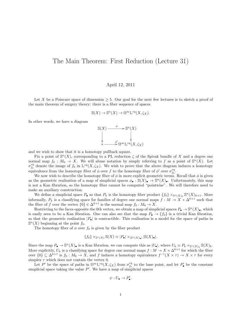
The Main Theorem: First Reduction (Lecture 31)

April 12, 2011

Let X be a Poincare space of dimension ≥ 5. Our goal for the next few lectures is to sketch a proof ofthe main theorem of surgery theory: there is a fiber sequence of spaces

S(X)→ Sn(X)→ Ω∞Lvq(X, ζX).

In other words, we have a diagram

S(X)φ //

Sn(X)

∗

φ′// Ω∞Lvq(X, ζX)

and we wish to show that it is a homotopy pullback square.Fix a point of Sn(X), corresponding to a PL reduction ζ of the Spivak bundle of X and a degree one

normal map f0 : M0 → X. We will abuse notation by simply referring to f as a point of Sn(X). Letσvqf0 denote the image of f0 in Lvq(X, ζX). We wish to prove that the above diagram induces a homotopy

equivalence from the homotopy fiber of φ over f to the homotopy fiber of φ′ over σvqf0 .We now wish to describe the homotopy fiber of φ in more explicit geometric terms. Recall that φ is given

as the geometric realization of a map of simplicial spaces φ• : S(X)• → Sn(X)•. Unfortunately, this mapis not a Kan fibration, so the homotopy fiber cannot be computed “pointwise”. We will therefore need tomake an auxiliary construction.

We define a simplicial space P• so that Pk is the homotopy fiber product f0 ×Sn(X)0 Sn(X)k+1. More

informally, Pk is a classifying space for families of degree one normal maps f : M → X × ∆k+1 such thatthe fiber of f over the vertex 0 ∈ ∆k+1 is the normal map f0 : M0 → X.

Restricting to the faces opposite the 0th vertex, we obtain a map of simplicial spaces P• → Sn(X)•, whichis easily seen to be a Kan fibration. One can also see that the map P• → f0 is a trivial Kan fibration,so that the geometric realization |P•| is contractible. This realization is a model for the space of paths inSn(X) beginning at the point f0.

The homotopy fiber of φ over f0 is given by the fiber product

f0 ×Sn(X) S(X) ' |P•| ×|Sn(X)•| |S(X)•|.

Since the map P• → Sn(X)• is a Kan fibration, we can compute this as |U•|, where Uk ' Pk ×Sn(X)k S(X)k.

More explicitly, Uk is a classifying space for degree one normal maps f : M → X ×∆k+1 for which the fiberover 0 ⊆ ∆k+1 is f0 : M0 → X, and f induces a homotopy equivalence f−1(X × τ) → X × τ for everysimplex τ which does not contain the vertex 0.

Let P ′ be the space of paths in Ω∞Lvq(X, ζX) from σvqf0 to the base point, and let P ′• be the constantsimplicial space taking the value P ′. We have a map of simplicial spaces

ψ : U• → P ′•.

1

To prove the main theorem, it will suffice to show that this map induces a homotopy equivalence of geometricrealizations. In fact, we claim that ψ is a trivial Kan fibration of simplicial spaces. In other words, we claimthat for each k ≥ 0, the canonical map

θk : Uk → U•(∂∆k)×Map(∂∆k,P ) Map(∆k, P )

is surjective on connected components.Let us spell out this out more explicitly in the special case k = 0. The space U0 classifies degree one

maps f : M → X×∆1 such that f−1(X×0) 'M0 and M1 = f−1(X×1) is homotopy equivalent to X.In other words, U0 is a classifying space for normal bordisms from M0 to a manifold homotopy equivalentto X. Every such bordism determines a Lagrangian in the Poincare object representing σvqf0 , which we can

regard as a path from σvqf0 to the base point in Ω∞Lvq(X, ζX). This path is the image of M under the mapθ0. Consequently, when k = 0, we wish to prove the following:

Theorem 1. Let X be a Poincare space of dimension n ≥ 5 equipped with a PL reduction of its tangent bun-dle, let f0 : M0 → X be a degree one normal map determining a Poincare object σvqf0 of (Shvlc(X; Sp)fp, QqζX ),

and let L be a Lagrangian in σvqf0 . Then L is cobordant to a Lagrangian arising from a normal bordism fromf0 : M0 → X to a homotopy equivalence f1 : M1 → X.

Let us now extend our analysis to the case where k is arbitrary. Let D ⊆ ∆k+1 be the subset obtainedby deleting the interior and the face opposite the 0th vertex. Then D is a PL disk equipped with preferredtriangulation. Every point of U•(∂∆k) determines D-family of normal maps f : M → X ×D such that thefiber over the vertex 0 ⊆ ∆k+1 (which we can think of as the “center” of the disk D) is given by M0,and f−1(X × τ) is homotopy equivalent to X × τ for every simplex τ ⊆ ∂ D. Such data determines a mapu : D → Ω∞Lvq(X, ζX) which is trivial on ∂ D (and carries the center of D to the point σvqf0 , but this is not

important in what follows). We may think of u as a point of Ω∞+kLvq(X, ζX), which we can represent byPoincare object (F, q) of (Shvlc(X; Spfp,ΩkζX).

Lifting f to a point of Uk amounts to extending f to a ∆k+1-family of normal maps f : M → X ×∆k+1,

such that f−1

(X × τ) is homotopy equivalent to X × τ for every face τ ⊆ ∆k+1 not containing the 0thvertex. Such an extension can be described by first specifying the inverse image of the face of ∆k+1 oppositethe 0th vertex: this is a PL manifold N equipped with a homotopy equivalence g : N → X ×∆k (neat over∆k) such that g−1(X × ∂∆k) is PL homeomorphic to f−1(X × ∂ D), together with a normal bordism fromM to N which is compatible with the PL homeomorphism on the boundaries.

Such a lifting determines an extension of σvqf to a map σvqf

: ∆k+1 → Ω∞Lvq(X, ζX) which vanishes

on the face of ∆k+1 opposite the 0th vertex. In particular, we obtain a Lagrangian in the Poincare object(F, q), which is well-defined up to bordism. Unwinding the definitions, the surjectivity of θk amounts to thefollowing assertion: every Lagrangian in (F, q) arises (up to cobordism) from a normal bordism from M toN as in the above paragraph.

It is convenient to rephrase the above construction by replacing the Poincare space X by the Poincarepair (X × D,X × ∂ D). Note that the Spivak bundle ζX×D is given by p∗(ΩkζX), where p denotes theprojection X ×D → X.

Let now embark on a brief digression about how some of the constructions of the last few lecturesgeneralize to the setting of Poincare pairs. Our definition of a degree one structure on a map of Poincarespaces f : Y → X generalizes to the setting of a map of Poincare pairs f : (Y, ∂ Y ) → (X, ∂ X). To such amap, one can assign a signature

σvqf : S → Lvq(X, ∂ X, ζX) = cofib(Lvq(∂ X, ζX | ∂ X)→ Lvq(X, ζX).

We have a fiber sequence of spectra

Lvq(X, ζX)→ Lvq(X, ∂ X, ζX)→ Lvq(∂ X, ζ∂ X),

2

where the second map carries σvqf to σvq∂ f , where ∂ f : ∂ Y → ∂ X denotes the induced degree one map ofPoincare spaces. In the special case where ∂ f is a homotopy equivalence, we obtain a canonical lifting ofσvqf to a point of Ω∞Lvq(X, ζX).

Let us now return to the problem of showing that the map

θk : Uk → U•(∂∆k)×Map(∂∆k,P ) Map(∆k, P )

is surjective. A point of the codomain determines a degree one normal map of Poincare pairs f : (M,∂M)→(X × D,X × ∂ D) which is a homotopy equivalence on the boundary, The relative signature σvqf can beidentified with the map u under the homotopy equivalence Lvq(X ×D, ζX×D) ' Lvq(X, ζX). Consequently,verifying the surjectivity of θk amounts to verifying that Theorem 2 is satisfied, where we replace the Poincarespace X by the Poincare pair (X ×D,X × ∂ D). This is in turn a special case of the following more generalassertion:

Theorem 2. Let (X, ∂ X) be a Poincare pair of dimension n ≥ 5 equipped with a PL reduction of itsSpivak bundle, let f : (M,∂M) → (X, ∂ X) be a degree one normal map inducing a homotopy equivalence∂M → ∂ X, and let L be a Lagrangian in Poincare object representing σvqf . Then L is cobordant to aLagrangian which arises from a normal bordism (constant along ∂M) from M to a homotopy equivalenceg : (N, ∂M)→ (X, ∂ X).

Remark 3. Using Theorem 2, we can extend the statement of the main theorem of the previous lecture tothe case of Poincare pairs. That is, if (X, ∂ X) is a Poincare pair of dimension n ≥ 5 where ∂ X is a PLmanifold of dimension n− 1, then we have a fiber sequence

S(X)→ Sn(X)→ Lvq(X, ζX).

3

Surgery (Lecture 32)

April 14, 2011

Our goal today is to begin the proof of the following:

Theorem 1. Let X be a Poincare pair of dimension n ≥ 5, ζ a stable PL bundle on X, and f : M → Xa degree one normal map, where M is a PL manifold. Let σvqf ∈ Ω∞Lvq(X, ζX) be the relative signature

of f , and suppose we are given a path p from σvqf to the base point of Ω∞Lvq(X, ζX). (We can identify

such a path with a Lagrangian in the Poincare object representing σvqf , which is well-defined up to bordism).

Then there exists a ∆1-family of degree one normal maps F : B → X × ∆1, where B is a bordism fromM = F−1(X × 0) to a PL manifold N = F−1(X × 1) such that F induces a homotopy equivalencef ′ : N → X. Moreover, we can arrange that F determines a path from σvqf to σvqf ′ = 0 which is homotopicto p.

Remark 2. In the last lecture, we sketched the formulation of a more general version of Theorem 1, wherewe replace X by a Poincare pair (X, ∂ X) where ∂ X is already a PL manifold. To simplify the discussion,we will restrict our attention to the case where ∂ X = ∅, but the ideas introduced in this lecture generalizeto the relative case.

To prove Theorem 1, we need a method for producing bordisms between PL manifolds. For this, we willuse the method of surgery. Fix a PL manifold M of dimension n. Write n = p+ q + 1. Let Dp+1 and Dq+1

denote PL disks of dimension p+ 1 and q + 1, respectively. Let Sp and Sq denote their boundaries (spheresof dimension p and q, respectively.

Definition 3. A p-surgery datum on M is a PL embedding α : Sp ×Dq+1 →M .

To a first approximation, a p-surgery datum α on M is given by an embedding of PL manifolds α0 :Sp →M (given by restricting α to the product of Sp with the center of Dq+1). To obtain a surgery datumfrom α0, we must additionally specify that α0 extends to a PL homeomorphism between Sp ×Dq+1 and aneighborhood of the image of α0. Such a homeomorphism determines a smooth structure on M along theimage of α0, with respect to which α0 is a smooth embedding with trivialized normal bundle. Conversely,suppose we are given an embedding α0 : Sp →M and a smoothing of M along the image of α0, such that α0

is a smooth map. Then α0 has a normal bundle Nα0, and there is a neighborhood of α0(Sp) in M which is

diffeomorphic to the unit sphere bundle of Nα0. In particular, if Nα0

is trivial, we obtain a diffeomorphism(and therefore a PL homeomorphism) of a neighborhood of α0(Sp) with Sp ×Dq+1. This argument showsthat we can identify a p-surgery datum on M with three pieces of data:

(i) A PL embedding α0 : Sp →M .

(ii) A smoothing of M along the image of α0 (with respect to which α0 is a smooth map).

(iii) A trivialization of the normal bundle to α0 (as a vector bundle).

Construction 4. Let M be a PL manifold of dimension n = p + q + 1 and let α : Sp ×Dq+1 → M be ap-surgery datum. We let B(α) denote the polyhedron given by

(M × [0, 1])∐

1×Sp×Dq+1

(Dp+1 ×Dq+1).

1

Then B(α) is a PL manifold with boundary, given by the disjoint union of M × 0 and

N = M − (Sp × (Dq+1)o)∐

Sp×Sq

(Dp+1 × Sq).

We refer to N as the PL manifold obtained from M via surgery along α, and to B(α) as the trace of thesurgery.

More informally: N is the manifold obtained from M by removing the interior of Sp × Dq+1 (therebycreating a manifold with boundary Sp × Sq) and gluing on a copy of Dp+1 × Sq.

Remark 5. LetN be a PL manifold obtained from surgery on a PL manifoldM along a map α : Sp×Dq+1 →M . Then there is an evident embedding β : Dp+1 × Sq → N , which is a q-surgery datum in N . Performingsurgery on N along β recovers the manifold M .

We will be interested in using surgery to construct normal bordisms between normal maps to a Poincarecomplex. For this, we need a slight variation on Definition 3. Let M be a PL manifold, so that thestable normal bundle of M is classifies by a map χ : M → Z × BPL. If we are given a p-surgery datumα : Sp ×Dq+1 →M , then χ α extends canonically to a map γ : Dp+1 ×Dq+1 → Z× BPL.

Suppose now that X is a space equipped with a stable PL bundle ζ, and that we are given a normalmap f : M → X. Then ζ is classified by a map χX : X → Z× BPL, and the normal structure on f gives ahomotopy h0 : χ ' χX f .

Definition 6. In the situation above, a normal p-surgery datum on M consists of the following data:

(i) A p-surgery datum α : Sp ×Dq+1 →M .

(ii) A map β : Dp+1 ×Dq+1 → X extending f α.

(iii) A homotopy h from χX β to γ, extending the homotopy determined by h.

Given a normal p-surgery datum, we can use α to construct a bordism B(α) from M to a PL manifoldN , β to construct a map F : B(α) → X extending f : M → X, and h to endow F with the structure of a∆1-family of normal maps.

Remark 7. Let us think of a p-surgery datum on a PL manifold M as an embedding α0 : Sp →M , togetherwith a choice of trivial normal bundle to α0. If f : M → X is a degree one normal map, then to obtain anormal p-surgery datum we need to choose a nullhomotopy of the composite map (f α0) : Sp → X, whichis compatible with the nullhomotopy of the map

Spα0→M

f→ X → Z× BPL

determined by the choice of trivial normal bundle.

Let us now see what surgery can do for us in low degrees. Assume that X is a Poincare space of dimensionn ≥ 5, ζ a stable PL bundle on X, and f : M → X is a degree one normal map.

Let us begin by doing surgery in the case p = −1. In this case, Sp is empty and therefore a surgerydatum α : Sp ×Dq+1 → M is unique. To promote α to a normal surgery datum, we need to choose a mapβ : Dn+1 → X (up to homotopy, this a point x ∈ X), together with a trivialization of β∗ζ. Unwinding thedefinitions, we see that B(α) is the disjoint union (M × [0, 1])

∐Dn+1, regarded as a bordism from M to

M∐Sn. If we have chosen β and the trivialization of β∗ζ, then we can regard this as a normal bordism

from f to a map M∐Sn → X, whose restriction to Sn is determined by β. By performing surgeries of this

type, we can always arrange that the map M → X is surjective on connected components.Now suppose that f : M → X fails to be injective on connected components. Then we can choose two

points x, y ∈ M belonging to different components of M and a path joining f(x) to f(y). Choosing small

2

disks around the points x and y, we obtain a 0-surgery datum α : S0 ×Dn → M . A choice of path p fromf(x) to f(y) determines the datum (ii) required by Definition 6. We cannot always extend α to a normalsurgery datum: our choice of disks determines trivializations of the fibers ζf(x) and ζf(y), which may or maynot extend to a trivalization of ζ over the path p. However, the obstruction is slight by virtue of the following(non-obvious!) fact:

Claim 8. The fundamental group π1(Z × BPL) is isomorphic to Z/2Z. In other words, every orientation-preserving PL automorphism of Rn is isotopic to the identity, for n 0.

In fact, more is true: the map πi(Z × BO) → πi(Z × BPL) induces an isomorphism for i ≤ 6 and asurjection when i = 7 (using smoothing theory, this is equivalent to the assertion that there are no exoticsmooth structures on piecewise linear spheres of dimensions ≤ 6). In this lecture, we will need somethingmuch weaker: namely, that the above map is bijective for i ≤ 1 and surjective for i ≤ 2. Using smoothingtheory, this is equivalent to the (reasonably obvious) claim that there are no exotic smooth structures onspheres of dimension ≤ 1.

In our situation, we cannot necessarily extend an arbitrary α : S0×Dn →M to a normal surgery datum.However, we always do so after modifying α by applying an orientation-reversing automorphism to one ofthe disks Dn. After making this modification, we obtain a normal bordism from M to a PL manifold withfewer connected components. Applying this procedure finitely many tiimes, we may replace f : M → X bya degree one normal map which induces an isomorphism π0M → π0X.

Let us now assume that X and M are connected, and choose a base point x ∈M . Suppose that the mapπ1M → π1X is not surjective. Choose another point y in M and a path q from y to x. Choose any class γin π1X, and a path p from f(x) to f(y) such that the loop composing p with f(q) represents γ. Choosingsmall disks around x and y, we obtain a surgery datum α : S0 ×Dn → M as before. The path p suppliesthe datum (ii) required by Definition 6, and we can argue as before (modifying α if necessary) to obtainthe datum (iii). Let N be obtained from M by normal surgery along α. Since n ≥ 3, deleting small disksaround x and y does not change the fundamental group of M . Using van Kampen’s theorem, we computethat π1N is obtained from π1M by freely adjoining an additional generator, and the map π1N → π1Xcarries this generator to γ (here we are being sloppy about base points here). Since X is a finite complex,its fundamental group is finitely generated. We may therefore perform this procedure finitely many times toreduce to the situation where the degree one normal map f : M → X induces a surjection π1M → π1X.

Now suppose that π1M → π1X fails to be injective. Choose an element of π1M whose image in π1Xis trivial. We can represent this element by a map α0 : S1 → M . Since the dimension of M is ≥ 3, ageneral position argument allows us to assume that α0 is an embedding. The composite map S1 →M → Xis nullhomotopic, so that the stable normal bundle of M is trivial in a neighborhood of α0 and we maytherefore assume that M is smooth in a neighborhood of α0. The normal bundle to α0 is stable trivial, henceorientable and therefore trivial. We may therefore extend α0 to an embedding α : S1×Dn−1 →M . Choosea nullhomotopy of f α. As before, it is not clear that we can choose datum (iii) required by Definition6: we encounter an obstruction in π2(Z × BPL). However, since the map π2(Z × BO) → π2(Z × BPL) issurjective, we can adjust our original embedding α (choosing a different trivialization of the normal bundleto α0) to make this obstruction vanish. This allows us to perform a normal surgery on the manifold M ,thereby obtaining a cobordant degree one normal map f ′ : N → X. Since the dimension of M is ≥ 4,removing a neighborhood of α0(S1) does not change the fundamental group of M . Consequently, we canuse van Kampen’s theorem to compute the fundamental group of N : it is obtained from the fundamentalgroup of M by killing the normal subgroup generated by γ.

Since X is a finite complex, the fundamental group π1X is finitely presented. Since π1M is finitelygenerated, the surjective map π1M → π1X exhibits π1X as the quotient of π1M by the normal subgroupgenerated by finitely many elements of π1M . It follows that, after a finite number of applications of theabove procedure, we may replace f : M → X by a degree one normal map which induces an isomorphism offundamental groups.

3

(Geometric) Surgery Below the Middle Dimension (Lecture 34)

April 20, 2011

In the last lecture, we reduced the main theorem of this course to the following assertion:

Theorem 1. Let X be a Poincare space of dimension n ≥ 5, let ζ be a stable PL bundle on X, and letf : M → X be a degree one normal map, where M is a compact PL manifold. Assume that M and X areconnected and that f induces an isomorphism π1M ' π1X ' G, so that σvqf can be represented by a Poincare

object (V, q), where V ∈ LModZ[G] satisfies C∗(M ;Z) ' C∗(X;Z) ⊕ ΣnV (here M and X denote universalcovers of M and X, respectively).

Assume that f is p-connected, that we are given a map u : Σp−nZ[G]→ V a nullhomotopy of q|Σp−nZ[G],so that (algebraic) surgery along u determines a bordism bordism from (V, q) to another Poincare object(V ′, q′). Then this (algebraic) bordism can be obtained by performing (geometric) surgery with respect to anormal surgery datum α : Sp ×Dq+1 →M .

In this lecture, we will treat the “easy” case of Theorem 1, where p is strictly smaller than n2 . Let

f : M → X be as in Theorem 1. Assume that f is p-connected, and choose any map e : ΣpZ[G] → ΣnV ,

classified by an element of πp−nV ' ker(Hp(M ;Z) → Hp(X;Z)) = Hp+1(X, M ;Z). Since f is p-connected,

the Hurewicz theorem allows us to identify this group with the relative homotopy group πp+1(X, M): that

is, with πpF , where F denotes the homotopy fiber of the map f : M → X (note that F can also be identifiedwith the homotopy fiber of the map f : M → X. Consequently, e determines a map α0 : Sp →M , togetherwith a nullhomotopy of the composite map Sp →M → X.

Since p < n2 , we can assume (modifying the map e by a homotopy if necessary) that α0 is an embedding.

Note that we have an equivalence of stable PL bundles

α∗0(−TM ) ' e∗f∗ζ.

Since the composition f α0 is nullhomotopic, we can trivialize the (stable) tangent bundle of M in aneighborhood of the image of α0. It follows from smoothing theory that M admits a smooth structure ina neighborhood U of α0(Sp), and this smooth structure admits a framing. Modifying α0 by a homotopy ifnecessary, we may assume that it is a smooth embedding from Sp into U . This embedding has a normalbundle, which we will denote by E. Since U and Sp are framed, the bundle E is framed: that is, it is stablytrivial. In order to extend α0 to a normal surgery datum α : Sp × Dn−p → M , we need to promote thisstable trivialization of E to an actual trivialization of E.

The bundle E is classified by a map χ : Sp → BO(n − p). Our stable framing gives a nullhomotopy

of the composite map Spχ→ BO(n − p) → BO(N) for N large. We wish to lift this to a nullhomotopy of

the map χ itself. We can carry out this lifting in stages. Suppose that we have a map ψ : Sp → BO(k)and a trivialization of the composite map Sp → BO(k) → BO(k + 1). This nullhomotopy determines afactorization of ψ through the homotopy fiber of the map BO(k)→ BO(k+1), which is homotopy equivalentto the quotient O(k+ 1)/O(k) ' Sk. If p < k, such a map is automatically nullhomotopic, and therefore thelifting is possible. This analysis applies in our case of interest: for any k ≥ n − p, we have p ≤ k, since wehave assumed that 2p < n.

The above argument shows that every map e : ΣpZ[G] → ΣnV can be lifted to a map α0 : Sp → Mwhich extends to a normal surgery datum α : Sp × Dn−p → M . However, this is not quite sufficient to

1

prove Theorem 1. A normal surgery datum determines both a map e : ΣpZ[G]→ ΣnV and a nullhomotopyof q|Σp−nZ[G]. In the situation of Theorem 1, there is generally no guarantee that this coincides with thenullhomotopy we are interested in.

Note that q|Σp−nZ[G] can be identified with a point in the 0th space of the spectrum

Σ−nQq(Σp−nZ[G]) = Σ−n(Σ2n−2pZ[G])hΣ2 = Σn−2p(Z[G])hΣ2 ,

where on the right hand side the permutation group acts on Z[G] by means of the involution of the previouslecture together with the sign (−1)n−p. Since n > 2p, this spectrum is always connected. If n > 2p+ 1, thisspectrum is simply connected: it follows that a nullhomotopy of q|Σp−nZ[G] is uniquely determined, up tohomotopy. This completes the proof of Theorem 1 in this case.

If n = 2p+ 1, we need to work a little bit harder. Let T be the set of homotopy classes of trivializationsof q|Σp−nZ[G]. Then T is a torsor for the group π1Σ−nQq(Σp−nZ[G]) ' Z[G]Σ2

, where Σ2 acts on thegroup Z[G] as indicated above. In particular, there is a transitive action of the group ring Z[G] (regardedas an abelian group under addition) on the set T . If α : Sp ×Dn−p →M is a normal surgery datum whoserestriction α0 to Sp × 0 represents the homology class e ∈ πp−nV , then α determines a nullhomotopy ofq|Σp−nZ[G]. Let us denote the corresponding element of T by t(α). To prove Theorem 1, it will suffice toshow that for any element x ∈ Z[G], we can find another normal surgery datum α′ (still representing thehomology class e) such that t(α′) = x + t(α). Since Z[G] is generated as abelian group by the elements ofG, we may assume that x = ±g, for some element g ∈ G. In this case, we assert without proof that there isa specific geometric construction for obtaining the surgery datum α′ (it is determined by writing an isotopythrough immersions from α0 to another embedding α′0). (Some pictures are provided in class; we will notreproduce them here.)

2

Surgery in the Middle Dimension (Lecture 35)

April 22, 2011

Recall that our goal is to prove the following:

Theorem 1. Let X be a Poincare space of dimension n ≥ 5, let ζ be a stable PL bundle on X, and letf : M → X be a degree one normal map, where M is a compact PL manifold. Assume that M and X areconnected and that f induces an isomorphism π1M ' π1X ' G, so that σvqf can be represented by a Poincare

object (V, q), where V ∈ LModZ[G] satisfies C∗(M ;Z) ' C∗(X;Z) ⊕ ΣnV (here M and X denote universalcovers of M and X, respectively).

Assume that f is p-connected, that we are given a map u : Σp−nZ[G]→ V a nullhomotopy of q|Σp−nZ[G],so that (algebraic) surgery along u determines a bordism bordism from (V, q) to another Poincare object(V ′, q′). Then this (algebraic) bordism can be obtained by performing (geometric) surgery with respect to anormal surgery datum α : Sp ×Dq+1 →M .

In the last lecture, we explained why this was true in the case where p < n2 . Our goal in this lecture is

sketch the proof in the case p = n2 . Let us therefore assume that n = 2k, that f is k-connected, and that we

are given a class u : Σ−kZ[G] → V and a nullhomotopy of q|Σ−kZ[G]. We would like to lift this data to anormal surgery datum in M .

Recall that, in order to identify Lvq(X, ζX) with Σ−nLq(Z[G]), we chose a base point of X and atrivialization of the Spivak bundle of X at the base point. Without loss of generality, we may suppose thatthis base point is the image a point x0 ∈ M , that G is given canonically as π1(M,x0), and that x0 is the

base point used in constructing the universal cover M (so that x0 lifts canonically to a point x0 ∈ M). Thetrivialization of ζX at f(x0) gives an orientation of the manifold M at the point x0, hence an orientation of

M at the point x0 (which extends to an orientation of the whole of M , since M is simply connected). We

have a group homomorphism ε : G→ ±1, where ε(g) = 1 if the action of G on M preserves the orientation,and ε(g) = −1 otherwise.

Let us now try to lift the class u to a normal surgery datum in X. The first step in the argument proceedsjust as in the previous lecture. Since f is k-connected, we can apply the relative Hurewicz theorem to thepair (X,M) to represent u by a diagram

Sk //

α0

M

Dk+1 // X.

Let α0 : Sk →M be the composition of α0 with the covering map M →M .We now encounter our first difficulty: since n = 2k, we cannot use general position arguments to ensure

that the map α0 : Sk → M is an embedding. However, we get almost this much for free: we can assumethat α0 is an immersion with a finite number of points of simple self-intersection. Then α0 is factors as acomposition

Skβ→ U →M,

1

where the map U →M is a local homeomorphism and β is both an embedding and a homotopy equivalence.Since f α0 is canonically nullhomotopic, the pullback β∗ − TM is trivialized, so that −TM is trivial alongU . In particular, we can assume that U is equipped with a smooth structure (and a framing). Modifying βby a homotopy if necessary, we may assume that β is a smooth embedding with normal bundle E, classifiedby a map Sk → BO(k). Using the framings of Sk and U , we obtain a nullhomotopy of the composite mapSk → BO(k)→ BO. Arguing as in the previous lecture, we can lift this to a nullhomotopy of the compositemap Sk → BO(k) → BO(k + 1). Such a nullhomotopy cannot always be lifted to a trivialization of E: weencounter an obstruction given by a map Sk → O(k + 1)/O(k) ' Sk, which has some degree d ∈ Z. Whenk is even, this integer is half of the Euler class of E; when k is odd, the integer d is really only well-definedmodulo 2 (that is, the exact integer d depends on a choice of trivialization of E⊕R). In either case, we canget the obstruction to vanish by introducing some “kinks” in the map β (that is, by replacing β by a mapwhich is homotopic but not isotopic to β, possibly introducing some additional double points). By means ofthis procedure, we can ensure that the stable framing of E lifts to a trivialization of E.

If the map α0 were an embedding, then (possibly after shrinking U) we can identify U with an open subsetof M , and the above argument allows us to extend α0 to a normal surgery datum α : Sk×Dk →M . However,α0 is generally not an embedding: we certainly cannot arrange this for an arbitrary map u : Σ−k → V . Wemust take advantage of the algebraic information encoded in the nullhomotopy of q|Σ−kZ[G]. Note thatq|Σ−kZ[G] can be regarded as a point of the space Ω∞+2kQq(Z[G]) = Ω∞(Z[G])hΣ2

. Here the action ofthe permuation group Σ2 on Z[G] is given by g 7→ (−1)kε(g)g−1, and the group of connected componentsof Ω∞(Z[G]) is given by the abelian group of coinvariants Z[G]Σ2 . The homotopy class of q|Σ−kZ[G] is anelement of this abelian group depending on u; let us denote it by q(u).

Let us describe the image of q(u) under the norm map

tr : Z[G]Σ2→ Z[G]Σ2 ⊆ Z[G].

Unwinding the definition, we see that this is given by restricting the Z[G]-valued intersection form on

C∗(M ;Z) along u. In particular, we have tr(q(u)) =∑g∈G j(g)g, where j(g) is the number of points of

intersection (counted with multiplicity) of α0(Sk) with its translate under g. Let us describe this numbermore explicitly. Let Y ⊆ Sk be the (finite) set of points over which α0 : Sk →M fails to be an immersion. Foreach y ∈ Y , there exactly one other element y ∈ Y such that α0(y) = α0(y). We then have α0(y) = gyα0(y)

for some element gy ∈ G. Moreover, the orientations of Sk at y and y determine an orientation of M at

α0(y). Define η(y) ∈ ±1 so that η(y) = 1 if this orientation agrees with our given orientation on M , andη(y) = −1 otherwise. Note that g(y) = g(y)−1, and that η(y) = (−1)kε(g(y)) (the first sign comes fromthe fact that permuting the factors of Rk ×Rk is orientation-reversing when k is odd, and the second fromthe fact that translation by g(y) is orientation-reversing when ε(g(y)) = −1). Unwinding the definitions(and using the triviality of the normal bundle E), we see that the self-intersection of the homology classrepresented by α0 is given by the expression

E =∑y∈Y

η(y)g(y).

Note that∑y∈Y η(y)g(y) =

∑y∈Y η(y)(−1)kε(g(y))g(y)−1. In particular, this sum is invariant under the

involution g 7→ (−1)kε(g)g−1, on Z[G], as we know it must be.We now observe that E lies in the image of the transfer map tr : Z[G]Σ2

→ Z[G]Σ2 . Namely, choosea decomposition Y = Y−

∐Y+, where for every element y ∈ Y exactly one of the points y, y belongs to

Y−. Then write E0 =∑y∈Y−

η(y)g(y). Then E0 ∈ Z[G] determines an element of Z[G]Σ2, whose transfer is

given by E. The specific element E0 ∈ Z[G] depends on the choice of decomposition Y = Y− ∪ Y+, but itsimage in Z[G]Σ2

does not.We assert the following without proof:

Claim 2. The element E0 defined above is a representative for q(u) ∈ Z[G]Σ2 .

2

Remark 3. When X is simply connected and n is divisible by 4, the transfer map tr : Z[G]Σ2' Z →

Z ' Z[G]Σ2 is injective (it is given by multiplication by 2), so that Claim 2 follows from our analysis of theintersection pairing).

Let us now study the meaning of the condition that q(u) = 0. Let G(2) ⊆ G be the subset consisting of 2-

torsion elements. Write G(2) = G−(2)∪G+(2), where g ∈ G+

(2) if (−1)kε(g) = 1, and g ∈ G−(2) if (−1)kε(g) = −1.

Choose a subset H ⊆ G −G(2) such that for every element g ∈ G which is no 2-torsion, exactly one of theelements g, g−1 belongs to H. Then Z[G]Σ2 is given by the direct sum

(⊕g∈H

Zg)⊕ (⊕g∈G+

(2)

Zg)⊕ (⊕g∈G−

(2)

Z/2Zg).

We may assume that Y− is chosen such that for y ∈ Y+, if g(y) is not 2-torsion, then g(y) ∈ H. Thenq(u) = 0 implies the following:

(i) If g ∈ H, then the sum∑y∈Y−,g(y)=g η(y) vanishes.

(ii) If g ∈ G+(2), then the sum

∑y∈Y−,g(y)=g η(y) vanishes.

(iii) If g ∈ G−(2), then the sum∑y∈Y−,g(y)=g η(y) is even.

Note that when g(y) ∈ G−(2), then replacing y by y changes the sign η(y). We therefore see that q(u) = 0 if

and only if we can choose Y− such that the sum E0 vanishes. In this case, we can partition Y into subsetsof the form y, y, y′, y′ where g(y) = g(y′) and η(y) = −η(y′).

The argument now proceeds by invoking Whitney’s trick for cancelling double points. Suppose we aregiven a quadruple y, y, y′, y′ as above. Choose a path γ from y to y′ in Sp, and another path γ from y′

to y. We may assume that the paths γ and γ are embedded, do not intersect one another, and do not meetany points of Y except at their endpoints.

After applying the map α0, we obtain paths in M which can be concatenated to yield a closed loop.The condition that g(y) = g(y′) implies that this loop is nullhomotopic (it lifts a loop in M , given byconcatenating α0(γ) with the translate by g(y)−1 of α0(γ)). We may therefore represent this loop by therestriction to the boundary of a continuous map D2 → M . Since the dimension of M is at least 5 (in fact,at least 6, since n = 2k is even), we may assume that the map D2 → M is an embedding which does notintersect the image of α0 except at the boundary. By analyzing a small neighborhood of the image of D2, wecan “push” the immersion α0 to obtain a new (isotopic) immersion, in which the double points y, y′, y, y′have been eliminated. Iterating this procedure, we can reduce to the case where Y = ∅, so that α0 is anembedding as desired.

The above analysis allows us to construct a normal surgery datum α : Sk ×Dk → M representing anymap u : Σ−kZ[G] → V such that q(u) = 0. However, this is not quite enough to prove Theorem ??. LetT denote the collection of homotopy classes of trivializations of q|Σ−kZ[G]. Then T is a torsor for thefundamental group π1Ω∞+nQq(Σ−kZ[G]) ' H1(Σ2;Z[G]), where the permutation group Σ2 acts on Z[G] asindicated above. A simple calculation shows that this group is given by the direct sum A =

⊕g∈G+

(2)Z/2Z.

Every normal surgery datum α representing u determines a nullhomotopy of q|Σ−kZ[G], giving an elementt(α) ∈ T . In order to prove Theorem ??, we need to show that every element of T has the form t(α), forsome normal surgery datum α. For this, we need a procedure to modify a given normal surgery datum α tochange the invariant t(α) in a controlled way.

The above analysis suggests such a procedure. Let g ∈ G+(2). Suppose we begin with a fixed embedding

α0 : Sk → M . By “reversing” the Whitney trick described above, we can modify α0 by an isotopy toobtain an immersion α′0 : Sk →M which fails to be an embedding at a set of points y, y′, y, y′, satisfyingg(y) = g(y′) = g and η(y) = −η(y′). Since g = g−1 and (−1)kε(g) = 1, we have g(y) = g(y) and η(y) = η(y).We may therefore switch the roles of y and y in Whitney’s construction, to obtain a different isotopy from

3

α′0 to an embedding α′′0 . Since α0 and α′′0 are isotopic (though immersions), every normal surgery datumα extending α0 determines a normal surgery datum α′′ extending α′′0 . We assert that t(α) = t(α′′) + x,where x is a generator for the summand of A corresponding to the element g ∈ G. Since the collection ofsuch elements generate the abelian group A and A acts transitively on T , this claim completes the proof ofTheorem 1.

4

The Homotopy Groups of G/PL (Lecture 36)

April 25, 2011

Let X be a Poincare space of dimension n. Recall that the normal structure space Sn(X) is homotopyequivalent to Stn(X), which is given by the homotopy fiber of the map BPLX → Pic(S)X (which classifiesstable PL reductions of the Spivak normal bundle of X). The map BPL→ Pic(S) is a map of infinite loopspaces, whose fiber we denote by G/PL (here one should think of G = GL1(S) as the automorphism group ofthe sphere spectrum). Consequently, if nonempty, the normal structure space Stn(X) is homotopy equivalentto a torsor for the infinite loop space (G/PL)X . Our goal in this lecture is to describe the homotopy typeof G/PL.

More generally, if (X, ∂ X) is a Poincare pair such that ∂ X is a compact PL manifold, we can describeStn(X) as the homotopy fiber of the canonical map

BPLX → Pic(S)X ×Pic(S)∂ X BPL∂ X

(over the point classifying the Spivak bundle of X together with its PL reduction on ∂ X). Assume that thePL tangent bundle to ∂ X is stably trivial, and that this trivialization extends to a trivialization of the Spivakbundle of X. Then Sn(X) can be identified with the space of maps of pairs from (X, ∂ X) to (G/PL, ∗).Taking X = Dn and ∂ X = Sn−1, we obtain a canonical homotopy equivalence Stn(X) = ΩnG/PL.

Recall that in the above situation, we have a homotopy commutative diagram

S(X) //

Stn(X)

θn

∗ // Ω∞Lvq(X, ζX).

In the special case (X, ∂ X) = (Dn, Sn−1), the Spivak bundle ζX is the constant sheaf with value Σ−nS. SinceX is simply connected, it follows that Lvq(X, ζX) is given by Σ−nLq(Z). We therefore have Ω∞Lvq(X, ζX) =ΩnLq(Z), where Lq(Z) denotes the zeroth space of the spectrum Lq(Z).

Taking n = 0, we obtain a map θ : G/PL → Lq(Z). With a little bit of effort, one can show that allof the maps θn appearing above are induced by θ by passing to n-fold loop spaces. We would like to usethe map θ to obtain information about the homotopy type of G/PL. We will obtain this information bycombining two facts:

(a) If n ≥ 5, then we have a homotopy pullback diagram

S(Dn) //

Ωn(G/PL)

Ωnθ

∗ // ΩnLq(Z).

This is a special case of our main theorem.

(b) If n ≥ 5, the structure space S(Dn) is contractible.

1

Let us provide an argument for (b). Recall that the structure space S(Dn) is given as the geometricrealization of a simplicial space S(Dn)•. Let Y• be the constant simplicial space which consists of a singlepoint in each degree. We claim that the map S(Dn)• → Y• is a trivial Kan fibration. In other words, weclaim that for every integer k, the map S(Dn)k → S(Dn)•(∂∆k) is surjective on connected components.

When k = 0, this says that S(Dn) is nonempty: this is obvious, since Dn is already a PL manifold. Wenow give the proof when k = 1; the proof of the general case is the same. Suppose we are given an elementof S(Dn)•(∂∆1), consisting of two contractible PL manifolds M and M ′ having boundary Sn−1. To liftto a point of S(Dn)1 we must write an h-cobordism from M to M ′, trivial along Sn−1. This is equivalentshowing that the manifold M

∐Sn−1 M ′ bounds a contractible PL manifold of dimension n + 1. Since M

and M ′ are contractible, M∐Sn−1 M ′ is homotopy equivalent to a sphere Sn. Since n ≥ 5, the generalized

Poincare conjecture implies that M∐Sn−1 M ′ is PL homeomorphic to Sn, which bounds the disk Dn+1.

Remark 1. In fact, something much stronger is true: each of the spaces S(Dn)k is contractible. One canprove this by combining the generalized Poincare conjecture with the Alexander trick.

Warning 2. In proving (b), it is important that we work in the PL category rather than the smooth category.The smooth structure space of Dn is generally not contractible because of the existence of exotic spheres. Wecan appreciate the importance of the PL condition by examining Smale’s proof of the generalized Poincareconjecture. Let M be a manifold of dimension n which is homotopy equivalent to a sphere, and assumethat n ≥ 6 (the case n = 5 requires additional effort). Choose two distinct points x, x′ ∈ M , and let Dand D′ be disjoint small disks around x and x′, respectively. Let Mo be the manifold obtained by removingthe interiors of D and D′. The condition that M is homotopy equivalent to Sn guarantees that Mo is anh-cobordism from ∂ D to ∂ D′. The h-cobordism theorem then gives Mo ' Sn−1 × [0, 1]. If we work inthe PL category, we can recover M from Mo by “collapsing” the two ends, thereby obtaining M ' Sn. Inthe smooth category, this argument does not apply: given a manifold with a boundary sphere, there is nocanonical way to assign a smooth structure to the manifold obtained by the collapsing the sphere.

Combining observations (a) and (b), we conclude the following:

(c) If n ≥ 5, the homotopy fiber of the map Ωn(θ) : ΩnG/PL→ ΩnLq(Z) is contractible. In other words,the map

πiG/PL→ πiLq(Z)

is injective when i = 5, and bijective for i > 5.

In fact, we can do a little bit better. Since π5Lq(Z) is trivial, the fact that π5G/PL → π5L

q(Z) isinjective implies that π5G/PL is trivial. It follows that Ω5(θ) is a homotopy equivalence.

Combining (c) with our calculation of the homotopy groups Lqn(Z), we obtain the following:

Corollary 3. Let n ≥ 5. Then we have a canonical isomorphism

πnG/PL '

8Z if n = 4k

0 if n = 4k + 1

Z/2Z if n = 4k + 2

0 if n = 4k + 3.

Let us now turn our attention to calculating the homotopy groups of G/PL in low degrees. We havemaps

Z× BO→ Z× BPL→ Pic(S),

giving rise to a fiber sequence of spaces

PL/O → G/O → G/PL.

2

Smoothing theory gives an identification of πnPL/O with the collection of smooth structures on Sn (com-patible with the standard PL structure on Sn. It follows that the map

πnG/O → πnG/PL

is bijective provided that the PL spheres Sn and Sn−1 admit unique smoothings. This is true for n ≤ 6.We can use this observation to compute πnG/PL for small values of n, since the homotopy groups of

Pic(S) and Z× BO are known. Let us summarize them in the following table:

Z× BO Pic(S)

π5 0 0

π4 Z Z/24Z

π3 0 Z/2Z

π2 Z/2Z Z/2Z

π1 Z/2Z Z/2Z

π0 Z Z.

The map from the groups on the left to the groups on the right is given by the J-homomorphism. This mapis an isomorphism on π1 and π2 and a surjection on π4. We therefore obtain

πnG/PL =

24Z if n = 4

0 if n = 3

Z/2Z if n = 2

0 if n = 1

0 if n = 0.

The map πn(G/PL)→ πnLq(Z) is obviously an isomorphism if n = 1 or n = 3, since both sides vanish.

Let us show that it is an isomorphism when n = 2. Let M be an oriented surface equipped with a spinstructure (or “theta characteristic”). Using the spin structure, we can trivialize the tangent bundle of Moutside of a small disk D ⊆ M , thereby obtaining a degree one normal map f : M → D/∂ D ' S2,

which in turn represents an element in π0Sn(S2) ' π0(G/PL)S2 ' π2(G/PL). The choice of spin structure

determines a quadratic refinement q of the intersection form on H1(M ;Z/2Z), making H1(M ;Z/2Z) into anondegenerate quadratic space over the finite field F2 = Z/2Z. To prove that the map

Z/2Z ' π2(G/PL)→ π2Lq(Z) ' π2L

q(F2) 'W (F2) ' Z/2Z

is nontrivial, it suffices to show that we can choose M (and its spin structure) so that the quadratic space(H1(M ;F2), q) has Arf invariant 1. This is always possible. The collection of spin structures on M is a

3

torsor for H1(M ;F2). If q has Arf invariant 0, then we can modify its Arf invariant by modifying the spinstructure by an element v ∈ H1(M ;F2) satisfying q(v) = 1 (which always exists provided that the genus ofM is positive).

Let us now compute the mapπ4G/PL→ π4L

q(Z) = 8Z

determined by θ. Choose a map u : S4 → G/O, representing a generator of [u] ∈ π4G/O ' π4G/PL. Thenu determines a point of the structure space Stn(S4), corresponding to a PL (in fact smooth) 4-manifold Mequipped with a degree one normal map f : M → S4. By construction, the image of [u] in Lq4(Z) ' 8Z isthe difference of signatures σM − σS4 . Since the signature of S4 vanishes, this is just the signature of M .

The Hirzebruch signature formula shows that this is given by p1(TM )3 [M ].

Let v : S4 → BO represent a generator [v] ∈ π4 BO ' Z. Then the composite map S4 u→ G/O → BOrepresents 24[v]. Let us regard p1 as an element in the integral cohomology ring H4(BO;Z). Since f has

degree 1, we can identify p1(TM )[ M ] with −24v∗(p1) ∈ H4(S4;Z) ' Z (the sign comes from our convention

that the map u classifies the normal bundle, rather than the tangent bundle). It follows that the image of[u] is given by −8v∗(p1) ∈ 8Z.

To compute v∗(p1), let us identify S4 with the quaternionic projective space HP1, Then we can takev : HP1 → BO to classify the real vector bundle E underlying quaternionic line bundle O(1). In particular,E admits the structure of a complex vector bundle , so that

p1(E) = −c2(E⊗C) = −c2(E⊕E) = −c2(E)− c1(E)c1(E)− c2(E) = −2c2(E) = −2e(E),

where e denotes the Euler class of E. Since E admits a section having exactly one simple zero, we obtainv∗(p1) = −2.

Corollary 4. The map θ : (G/PL)→ Lq(Z) induces an isomorphism πn(G/PL)→ πnLq(Z) for all n 6= 0, 4.

The map π4(G/PL)→ π4Lq(Z) is injective, and its image is the subgroup 16Z ⊆ 8Z ' π4L

q(Z).

Remark 5. The failure of the map π4(G/PL) → π4Lq(Z) to be surjective is a consequence of Rohlin’s

theorem: a smooth, compact, spin 4-manifold M has signature divisible by 16.

We can regard Corollary ?? as a calculation of the homotopy groups of the homotopy fiber of the mapθ. Since these homotopy groups are concentrated in a single degree, the structure of the homotopy fiber canbe explicitly determined:

Corollary 6. We have a homotopy fiber sequence K(Z/2Z, 3)→ G/PL→ Lq(Z)

It is possibly to carry out many of the constructions of this course in the setting of topological manifolds(rather than PL manifolds). Stable topological bundles are classified by a space Z × BTOP fitting into adiagram

Z× BPL→ Z× BTOP→ Pic(S).

There is an associated fiber sequence Top /PL → G/PL → G/Top . The map G/PL → Lq(Z) factorsthrough G/Top, and G/Top is homotopy equivalent to the identity component of Lq(Z). Assuming this,Corollary 6 gives a homotopy equivalence Top /PL ' K(Z/2Z, 3). We therefore have a fiber sequence ofinfinite loop spaces

Z× BPL→ Z× BTOPφ→ K(Z/2Z, 4).

The map φ classifies the Kirby-Siebenmann obstruction. IfM is a topological manifold, its stable (topological)tangent bundle is classified by a map M → Z × BTOP. Composing this map with φ, we get a mapM → K(Z/2Z, 4), classified by a cohomology class ν ∈ H4(M ;Z/2Z). This class vanishes if and only ifthe stable tangent bundle of M admits a PL reduction. In particular, ν vanishes whenever M admits a PLstructure. One can show that the converse holds if the dimension of M is different from 4.

4

The Total Surgery Obstruction (Lecture 37)

April 27, 2011

Let X be a finite polyhedron, ζX a spherical fibration on X, and R and A∞-ring with involution. Recallthat we have a homotopy pullback diagram of spectra

Lq(X, ζX , R) //

Ls(X, ζX , R)

Lvq(X, ζX , R) // Lvs(X, ζX , R),

where the vertical maps are given by assembly. From now on, we will fix R to be the ring Z of integers, andomit it from the notation (we could just as well take R to be the sphere spectrum). Let L(X, ζX) denotethe cofibers of the horizontal maps, so that we have a diagram

Lq(X, ζX) //

Ls(X, ζX)

// L(X, ζX)

Lvq(X, ζX) // Lvs(X, ζX) // L(X, ζX).

When the spherical fibration ζX is trivial; we will omit it from the notation. If, in addition, X is a point,then the vertical maps are homotopy equivalences and we have a single fiber sequence

Lq(Z)→ Ls(Z)→ L.

The upper row of the diagram above consists of functors which are excisive in X. We may thereforewrite L(X, ζX) = C∗(X, L(ζX)), where L(ζX) is the local system on X which assigns to each point x ∈ Xthe spectrum L(ζX(x)).

Suppose we are given a map of spaces i : ∂ X → X. We let Lvs(X, ∂ X, ζX) denote the cofiber of the map

Lvs(∂ X, ζX | ∂ X) → Lvs(X, ζX), and define Lvq(X, ∂ X, ζX) and L(X, ∂ X, ζX) similarly. By functoriality,we obtain vertical maps fitting into a commutative diagram of spectra

Lq(Z) ∧ (X/∂ X) //

Ls(Z) ∧ (X/∂ X) //

L ∧ (X/∂ X)

Lvq(X, ∂ X) // Lvs(X, ∂ X) // L(X, ∂ X).

The right vertical map is a homotopy equivalence (by excision). If X and ∂ X have the same fundamentalgroupoid, then the π-π theorem implies that Lvq(X, ∂ X) vanishes. The above diagram then gives a canonicalhomotopy equivalence

L ∧ (X/∂ X) ' Lvs(X, ∂ X).

1

In particular, we can take X = Dn and ∂ X = Sn−1 for n ≥ 3, to obtain a homotopy equivalence

L ' ΩnLvs(Dn, Sn−1).

Recall that the symmetric L-theory spectrum Ls(Z) is an E∞-ring spectrum, with multiplication inducedby the tensor product of chain complexes. If we have pairs of spaces (X, ∂ X) and (Y, ∂ Y ), there is a similarmultiplicaiton

Lvs(X, ∂ X) ∧ Lvs(Y, ∂ Y )→ Lvs(X × Y, ∂(X × Y )),

where ∂(X ×Y ) denotes the homotopy pushout (∂ X ×Y )∐∂ X×∂ Y (X ×∂ Y ). Taking X and Y to be disks

of dimension ≥ 3, this gives a multiplication

L ∧ L→ L.

Using more elaborate reasoning along the same lines, we see that L also has the structure of an E∞-ringspectrum, and that the canonical map Ls(Z)→ L can be promoted to a map of E∞-ring spectra.

Now suppose that (X, ∂ X) is a Poincare pair with Spivak fibration ζX , so that the visible symmetric

signature σvsX ∈ Ω∞Ls(X, ∂X , ζX) is defined. Let σX denote the image of σvsX in Ω∞L(X, ∂ X, ζX).Let us now suppose that ∂ X = Sn−1 is a sphere, and that X = Dn is the cone on ∂ X. Then the Spivak

bundle of X is canonically equivalent to the constant sheaf whose value is an invertible specturm E, givenby the inverse of Σ∞(X/∂ X). Then L(X, ∂ X, ζX) can be identified with the spectrum E−1 ∧ L(∗, E). We

can then identify σX with a map L-modules φ : E ∧ L→ L(E), which is a homotopy equivalence. In Lecture23, we discussed an analogous homotopy equivalence

φ : E ∧ Ls(Z) ' Ls(∗, E).

These maps fit into a commutative diagram

E ∧ Ls(Z)φ //

Ls(∗, E)

E ∧ L

φ // L(∗, E).

However, there is an important difference: to write down the map φ, we needed to realize the spectrumLs(X, ∂ X,E) in terms of constructible sheaves on X; the map φ itself was given by choosing the constantsheaf on X, which is Verdier-self dual (up to a twist). Consequently, φ is functorial with respect to PL

homeomorphisms of X = Dn. However, the construction of φ depends only on the realization of (X, ∂ X)as a Poincare pair, and is therefore functorial with respect to all homotopy equivalences of ∂ X = Sn−1.

Elaborating on the above construction, we obtain the following:

Proposition 1. Let E be any invertible spectrum. Then there is a canonical homotopy equivalence

E ∧ L ' L(∗, E).

Now suppose we are given a point η ∈ G/PL = fib(Z × BPL → Pic(S)). Then η classifies a stable PLbundle ζ over a point, together with a trivialization of the underlying invertible spectrum E. Using ζ, wecan write down a homotopy equivalence of Ls-modules

φζ : E ∧ Ls(Z)→ Ls(∗, E).

Since E is trivial, we can think of φζ as an invertible map from Ls(Z) to itself. This construction gives amap

G/PL→ GL1(Ls(Z))

2

Since the automorphism of L determined by φζ depends only on the underlying spherical fibration of ζ, thisautomorphism is trivial. Consequently, the composite map

G/PL→ GL1(Ls(Z))→ GL1(L)

is canonically nullhomotopic. We therefore obtain a map G/PL→ F , where F denotes the homotopy fiber

of the map GL1(Ls)→ GL1(L). Note that F is the identity component of the space

Lq(Z) = Ω∞ fib(Ls → L).

The above construction recovers the map θ : G/PL→ Lq(Z) described in the previous lecture. Recall thatthis map is almost a homotopy equivalence: we have a fiber sequence K(Z/2Z, 3)→ G/PL→ Lq(Z).

Now let X be any finite polyhedron and ζX any spherical fibration on X. Using excision and Proposition1, we obtain homotopy equivalences

L(X, ζX) ' C∗(X; L(ζX)) ' C∗(X; ζX ∧ L).

Here L(ζX) denotes the local system on X which assigns to each point x ∈ X the spectrum L(x, ζX(x)).In the special case where X is a Poincare space and ζX is its Spivak bundle, we obtain

L(X, ζX) ' C∗(X; L).

Under this homotopy equivalence, the point σX ∈ Ω∞L(X, ζX) corresponds to the global section of L given

by the unit of L.A similar calculation gives Ls(X, ζX) ' C∗(X; ζ−1

X ∧ Ls(ζX)), where Ls(ζX) denotes the local systemon X which assigns to each point x ∈ X the spectrum Ls(x, ζX(x)). In other words, we can identifyLs(X, ζX) with the Mor(ζX ∧ Ls(Z),Ls(ζX)) in the ∞-category of local systems of Ls(Z)-modules on X.Let Ls(X, ζX)× denote the subspace of Ω∞Ls(X, ζX) corresponding to isomorphisms ζX ∧Ls(Z)→ Ls(ζX).We have a map

Ls(X, ζX)× → Ω∞L(X, ζX).

The homotopy fiber of this map over σX can be identified with the space of sections of a fibration X ′ → X,having fiber F = fib(GL1(Ls(Z))→ GL1(L)).

Any stable PL structure on the bundle ζX gives an isomorphism of local systems of Ls(Z)-modulesζX ∧Ls(Z)→ Ls(ζX), corresponding to a point of Ls(X, ζX)× ×Ω∞L(X,ζX) σX. The collection of such PL

structures is classified by the space of sections of a fibration X ×Pic(S) (Z×BPL)→ X, having fiber G/PL.We have a map of spaces over X

X ×Pic(S) (Z× BPL)→ X ′

having homotopy fiber K(Z/2Z, 3). Consequently, every section s of the map X ′ → X determines a fibrationY → X with fiber K(Z/2Z, 3), where Y = X ×X′ (X ×Pic(S) (Z × BPL)). This fibration is classified by amap X → K(Z/2Z, 4), which depends on the choice of section s. We therefore obtain a map

Ls(X, ζX)× ×Ω∞L(X,ζX) σX → K(Z/2Z, 4)X ,

whose fiber can be identified with the structure space Stn(X).Let S′(X) denote the homotopy fiber product Ls(X, ζX)× ×Ω∞Lvs(X,ζX) σvsX . Recall that if M is a

manifold equipped with a homotopy equivalence f : M → X, then f determines a lifting of σvsX , giving apoint of S′(X). Elaborating on this construction, we get a map S(X)→ S′(X), which fits into a commutativediagram

S(X) //

Sn(X) //

Ω∞Lvq(X, ζX)

S′(X) // Ls(X, ζX)× ×Ω∞L(X,ζX) σX // Ω∞Lvq(X, ζX).

3

Assume that the dimension of X is at least 5. The main theorem of this course asserts that the upper rowis a fiber sequence, and the bottom row is obviously a fiber sequence. Since the right vertical map is ahomotopy equivalence, we see that the square on the left is homotopy Cartesian. Combining this with theabove analysis, we obtain:

Theorem 2. Let X be a Poincare space of dimension ≥ 5. Then we have a fiber sequence of spaces

S(X)→ S′(X)→ K(Z/2Z, 4)X ,

where S′(X) = Ls(X, ζX)× ×Ω∞Lvs(X,ζX) σvsX .

Remark 3. It is possible to prove the main results of this course in the setting of topological, ratherthan piecewise linear manifolds. However, things work slightly differently in low degrees: we actually geta homotopy equivalence from G/Top to the base point component of Lq(Z). The analysis above showsthat S′(X) can be identified with the topological structure space of X, parametrizing h-cobordism classesof compact topological manifolds in the homotopy type of X. The map ψ : S′(X) → K(Z/2Z, 4)X is aversion of the Kirby-Siebenmann obstruction: it assigns to every topological manifold M of dimension ≥ 5 acohomology class η ∈ H4(M ;Z/2Z), which vanishes if and only if M admits a PL structure.

4