COVARIANCE FUNCTION MODELLING IN LOCAL GEODETIC … · using the Simplex Method. The procedure has been implemented in a FORTRAN95 software The procedure has been implemented in a

BCG - Boletim de Ciências Geodésicas - On-Line version, ISSN 1982-2170

http://dx.doi.org/10.1590/S1982-21702016000200019

Bol. Ciênc. Geod., sec. Artigos, Curitiba, v. 22, no2, p.342- 357, abr - jun, 2016.

Article

COVARIANCE FUNCTION MODELLING IN LOCAL GEODETIC

APPLICATIONS USING THE SIMPLEX METHOD

Modelagem da função covariância em aplicações geodésicas locais utilizando o

método simplex

Carlo Iapige De Gaetani 1

Noemi Emanuela Cazzaniga 1

Riccardo Barzaghi 1

Mirko Reguzzoni 1

Barbara Betti 1

1 Politecnico di Milano, Department of Civil and Environmental Engineering (DICA), Piazza Leonardo da Vinci 32, 20133 Milan, Italy

email: [email protected]; [email protected]; [email protected]; [email protected]; [email protected]

Abstract:

Collocation has been widely applied in geodesy for estimating the gravity field of the Earth both

locally and globally. Particularly, this is the standard geodetic method used to combine all the

available data to get an integrated estimate of any functional of the anomalous potential T. The

key point of the method is the definition of proper covariance functions of the data. Covariance

function models have been proposed by many authors together with the related software. In this

paper a new method for finding suitable covariance models has been devised. The covariance

fitting problem is reduced to an optimization problem in Linear Programming and solved by

using the Simplex Method. The procedure has been implemented in a FORTRAN95 software

and has been tested on simulated and real data sets. These first tests proved that the proposed

method is a reliable tool for estimating proper covariance function models to be used in the

collocation procedure.

Keywords: Local Disturbing Potential, Data Integration, Collocation, Covariance Functions,

Linear Programming, Simplex Method

Resumo:

A técnica de Colocação tem sido bastante aplicada em Geodésia para estimação do campo da

gravidade da Terra em ambos os aspectos, isto é, localmente e globalmente. Particularmente, este

é o método geodésico padrão usado para combinar todos os dados disponíveis para se obter uma

estimativa integrada de qualquer anomalia potencial T. A principal característica do método é a

definição da função covariância dos dados. Diversas funções covariância tem sido propostas na

literatura, juntamente, com o software relacionado. Neste trabalho, um novo método para

Gaetani, C. et al. 343

Bol. Ciênc. Geod., sec. Artigos, Curitiba, v. 22, no2, p.342-357, abr - jun, 2016.

determinar funções covariância é proposto. O problema de ajustamento da covariância é

reduzido para um problema de otimização em programação linear e solucionado pelo método

conhecido como Simplex. O método proposto foi implementado em linguagem de programação

FORTRAN95 e foi testado com dados simulados e reais. Os resultados obtidos mostraram que o

método proposto é uma potente ferramenta para estimação de modelos da função covariância e

pode ser empregado em técnicas de Colocação.

Palavras-chave: Potencial de Distúrbio Local; Integração de Dados; Colocação; Função

Covariânica; Programação Linear; Método Simplex.

1. Introduction

One of the standard procedures for local gravity field modelling is based on the combination of

the Remove-Restore technique (RR) (Sansò, 2013a) and Collocation method (Sansò, 2013b).

The RR principle is one of the most well-known strategies used for regional and local gravity

field determination. It is based on the assumption that gravity signals can be divided into long,

medium and short wavelength components. The long wavelength component can be properly

accounted for by Global Geopotential Models (GGM) that are estimated using satellite derived

observations and ground based gravity data (Pavlis et al., 2012). Removing the effect of a GGM

corresponds to a high-pass filtering of the data. In this reduction step, the gravity signals due to

the mean crust, the upper mantle and the long wavelength topographic signal are removed from

the observed values.

After reduction for a global model, in addition to medium frequencies, high frequency

components are still present in the residual data. They are essentially due to the high frequency

features of the topography which cannot be suitably described by global models (Forsberg,

1994). This residual topographic signal is then removed from the observed data by computing

the so called Residual Terrain Correction (RTC) (Forsberg, 1994). The residual data obtained by

applying both the reduction for the global model and the related RTC contain only the

intermediate wavelengths to be used for local gravity field modelling. They usually have a mean

value close to zero and a standard deviation that is remarkably smaller than the standard

deviation of the unreduced data. Collocation can be suitably applied to these reduced data to get

estimates of the local features of the gravity field (Tscherning, 2004). The final estimate is then

obtained by restoring the geopotential model and RTC effects which are added to this local

residual component in order to obtain the final full power estimate.

As mentioned, Collocation is applied to get the estimate of the residual local component of the

gravity signal. Collocation is a statistical-mathematical theory applied to gravity field modelling

problems (Heiskanen and Moritz, 1967; Moritz, 1980; Sansò, 2013b). It is based on the

assumption that the gravity observations can be considered as a realization of a weakly stationary

and ergodic stochastic process (Moritz, 1980, pp. 279-285). This theory has become more and

more important because it allows combining different kinds of gravity field observables in order

to obtain a better estimate of any linear functional of the anomalous potential T(P). With the

great amount of heterogeneous data nowadays available, this approach has been fully accepted as

the standard methodology for integrated gravity field modelling. The key point in Collocation is

the concept of spatial correlation which is described by the covariance function of the

observations. Being all the observed geodetic quantities (as g, N or Trr) linear(ized) functionals

344 Covariance function.…


of the anomalous gravity potential (T), it can be also proved (Moritz, 1980, pp. 86-87) that their

covariance functions can be propagated one to each other by applying the proper linear operators

to the well-known analytical model of covariance of the anomalous potential T(P).

In local geodetic applications, this model (Knudsen, 1987) is given by

1

12

2

2

12

2 coscos

redNn

PQn

n

QP

n

redN

n

PQn

n

QP

nPQ Prr

RTP

rr

RTeC (1)

where R is the radius of the Bjerhammar sphere, Pr and Qr are the geocentric radii of points P

and Q,2n are the degree variances,

2ne are the error degree variances, is a scale factor, nP are

the Legendre polynomials and PQ is the spherical distance between P and Q.

Such covariance model is the sum of two parts. The first comes from the commission error of the

global model removed from observations. It is given in terms of the sum of the error degree

variances 2ne up to the maximum degree of computation of the global model subtracted in the

remove phase. 2ne are computed as the sum of the variances of the estimated spherical harmonic

model coefficients, nmC2 and nmS2 (Pavlis et al., 2012):

n

m

nmnmn SCe0

222 (2)

So, error degree variances depend on the global model used and the coefficient in (1) allows

weighting their influence. The second part is related to the residual part of the signal. Suitable

models for Tn2 in (1) were proposed by Tscherning and Rapp (Tscherning and Rapp, 1974;

Tscherning, 2004)

Bnnn

AT

nn

AT

n

n

21

21

2

2

(3)

where A and B are model constants to be estimated. As stated, using covariance propagation,

these covariance models of the anomalous potential T can be used to get models for any

functional of T. By tuning the model constants (i.e. A, , R and B), these model functions can be

used to properly fit the empirical covariances of the available data.

In turn, the empirical covariance function of the observed data can be estimated using the

formula (Mussio, 1984):

j

n

j

i

m

i

llnm

kCC

11

11

2

(4)

where m is the number of li observations and n is the number of jl observations at spherical

distance ij from li so that

,...,kkkk ij 1 ,1 (5)

for a suitable value.



If homogeneous data are considered, formula (4) gives the empirical estimate of the auto-

covariance of these data. In case l and l’ are different functionals of T (e.g. g and N), (4) is the

empirical estimate of the cross-covariance between l and l’.

Once the covariance functions of the observed data are properly modeled, Collocation formula

can be applied to get the estimate of any functional of the anomalous potential T. As it is well

known, the general formula of Least Squares Collocation (LSC) giving the estimate is (Moritz,

1980, pp. 84-87; Sansò, 2013):

ii

N

jijTiTjiPTiTPiP TLICLLCLLTL

1,

12 ˆ (6)

where iL is the observed linear(ized) functional of T in Pi, jTiTji CLL is the covariance matrix of

observations, 2 is the variance of the observation noise , LP is the estimated linear functional

of T in P and I is the identity matrix.

This is the usual procedure for covariance function modelling and collocation estimate

computation. As it is evident, the covariance structure of the data plays a fundamental role in

getting the solution in equation (6). Thus, the correct modelling of the covariance functions is a

critical point in computing a reliable estimate.

The proposed models are sometimes unable to properly fit the empirical covariances, particularly

when different functionals are considered. In a previously proposed approach (Tselfes, 2008;

Barzaghi et al., 2009) regularized least squares adjustment have been applied for integrated

covariance function modelling which, however, can lead to negative Tn2 values that must be

rejected. Hence, this procedure must be iterated to get a final set of suitable Tn2 . In the next

section, a new covariance modelling procedure solving this problem will be described.

2. A new procedure for covariance modelling based on Linear

Programming

In order to overcome some limits of the method presented in Barzaghi et al. (2009), a covariance

fitting method based on linear programming is proposed.

Considering a system of linear inequalities of the following form (see also Figure 1):



0

0

0

a...aa

a...aa

a...aa

2

1

mn2m21m1

22n222121

11n212111

n

mn

n

n

x

x

x

bxxx

bxxx

bxxx

(7)

there are several sets of values nxxx ,..., 21 that are solutions to (7). Finding one of particular

interest is an optimization process (Press et al., 1989). When this solution is the one minimizing

(or maximizing) a given linear combination of the variables (called objective function)

min...2211 nnxcxcxc (8)

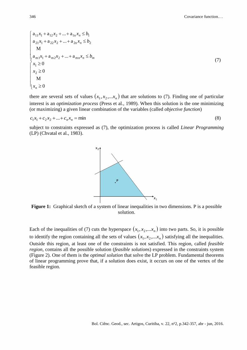
subject to constraints expressed as (7), the optimization process is called Linear Programming

(LP) (Chvatal et al., 1983).

Figure 1: Graphical sketch of a system of linear inequalities in two dimensions. P is a possible

solution.

Each of the inequalities of (7) cuts the hyperspace nxxx ,..., 21 into two parts. So, it is possible

to identify the region containing all the sets of values nxxx ,..., 21 satisfying all the inequalities.

Outside this region, at least one of the constraints is not satisfied. This region, called feasible

region, contains all the possible solution (feasible solutions) expressed in the constraints system

(Figure 2). One of them is the optimal solution that solve the LP problem. Fundamental theorems

of linear programming prove that, if a solution does exist, it occurs on one of the vertex of the

feasible region.



Figure 2: Example of two-dimensional feasible region of constraints

For applications involving a large number of constraints or variables, numerical methods must be

applied. One of them is the Simplex Method (Ficken, 1961). It provides a systematic way of

examining the vertices of the feasible region to determine the optimal value of the objective

function. The simplex method consists in elementary row operations on a particular matrix

corresponding to the LP problem called tableau. The initial version of the tableau changes its

form through iterative optimality checks. This operation is called pivoting. To form the improved

solution, Gauss-Jordan elimination is applied with the pivot (crossing pivot row and column) to

the column pivot. After improving the solution, the simplex algorithm starts a new iteration

checking for further improvements. The tableau changes at each iteration and the conditions of

optimality or unfeasibility of the solution to the proposed LP problem stop the algorithm. Based

on fundamental theorem of linear programming, simplex method is able to verify the existence

of at least one solution to the proposed LP problem. If this exists, the algorithm is also able to

find the best numerical solution in a finite amount of time.

Using this principle, a new covariance fitting procedure based on the simplex method and the

analytical covariance function model (1) has been devised. It applies simplex method for

estimating some suitable parameters of the model covariance function (1) in order to fit

simultaneously the empirical covariances of all the available data. One possible way of doing so

using the simplex method is to assume as a model covariance for the anomalous potential T a

slightly modified version of (1), i.e.

max

1

12

2

2

12

2 cos~cos~N

redNn

PQn

n

QP

n

redN

n

PQn

n

QP

nPQ Prr

RTP

rr

RTeC (9)

where 2~

ne , are the error degree variances of the model used for reducing the data in the remove

step and 2~n are some guess values for the degree variances.

2~n can be computed by using again

the applied geopotential model (in case Nred Nmax) or by describing them according to some

general rule, e.g. the Kaula’s rule (Kaula, 2000). The fitting procedure is then implemented

through the following conditions that allow estimating suitable values for and

min (10)



TLTLiemp

TLTLiTLTL

TLTLiemp

TLTLiTLTL

CCC

CCC

'''

'''

,,

,,

0

0

(11)

where iemp

TLTLC

' and iTLTL

C '

are, respectively, the empirical and the model covariances

related to the L(T) and L’(T) functionals.

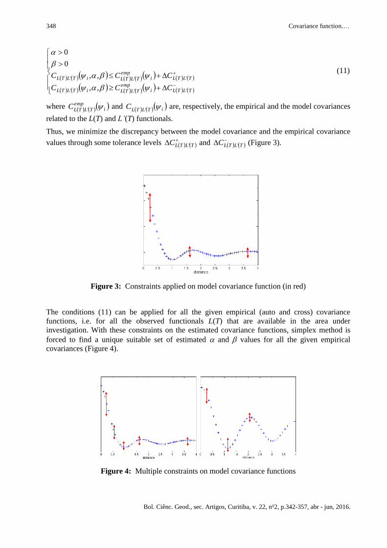
Thus, we minimize the discrepancy between the model covariance and the empirical covariance

values through some tolerance levels TLTLC ' and

TLTLC ' (Figure 3).

Figure 3: Constraints applied on model covariance function (in red)

The conditions (11) can be applied for all the given empirical (auto and cross) covariance

functions, i.e. for all the observed functionals L(T) that are available in the area under

investigation. With these constraints on the estimated covariance functions, simplex method is

forced to find a unique suitable set of estimated and values for all the given empirical

covariances (Figure 4).

Figure 4: Multiple constraints on model covariance functions



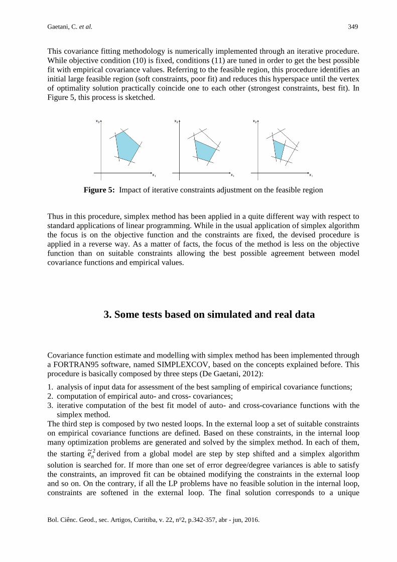
This covariance fitting methodology is numerically implemented through an iterative procedure.

While objective condition (10) is fixed, conditions (11) are tuned in order to get the best possible

fit with empirical covariance values. Referring to the feasible region, this procedure identifies an

initial large feasible region (soft constraints, poor fit) and reduces this hyperspace until the vertex

of optimality solution practically coincide one to each other (strongest constraints, best fit). In

Figure 5, this process is sketched.

Figure 5: Impact of iterative constraints adjustment on the feasible region

Thus in this procedure, simplex method has been applied in a quite different way with respect to

standard applications of linear programming. While in the usual application of simplex algorithm

the focus is on the objective function and the constraints are fixed, the devised procedure is

applied in a reverse way. As a matter of facts, the focus of the method is less on the objective

function than on suitable constraints allowing the best possible agreement between model

covariance functions and empirical values.

3. Some tests based on simulated and real data

Covariance function estimate and modelling with simplex method has been implemented through

a FORTRAN95 software, named SIMPLEXCOV, based on the concepts explained before. This

procedure is basically composed by three steps (De Gaetani, 2012):

1. analysis of input data for assessment of the best sampling of empirical covariance functions;

2. computation of empirical auto- and cross- covariances;

3. iterative computation of the best fit model of auto- and cross-covariance functions with the

simplex method.

The third step is composed by two nested loops. In the external loop a set of suitable constraints

on empirical covariance functions are defined. Based on these constraints, in the internal loop

many optimization problems are generated and solved by the simplex method. In each of them,

the starting 2~

ne derived from a global model are step by step shifted and a simplex algorithm

solution is searched for. If more than one set of error degree/degree variances is able to satisfy

the constraints, an improved fit can be obtained modifying the constraints in the external loop

and so on. On the contrary, if all the LP problems have no feasible solution in the internal loop,

constraints are softened in the external loop. The final solution corresponds to a unique



combination of shifted error degree variances 2~

ne , and values that allow to obtain the best

possible fit between empirical covariances and the model covariance functions.

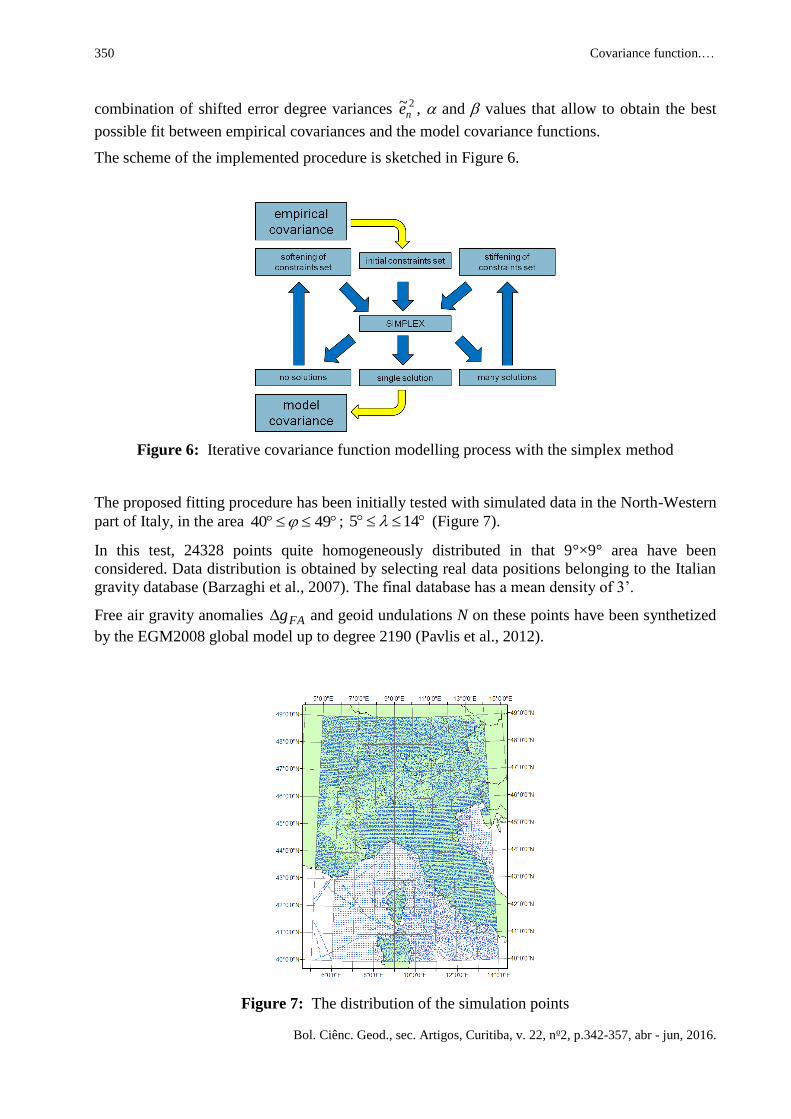
The scheme of the implemented procedure is sketched in Figure 6.

Figure 6: Iterative covariance function modelling process with the simplex method

The proposed fitting procedure has been initially tested with simulated data in the North-Western

part of Italy, in the area 4940 ; 145 (Figure 7).

In this test, 24328 points quite homogeneously distributed in that 9°×9° area have been

considered. Data distribution is obtained by selecting real data positions belonging to the Italian

gravity database (Barzaghi et al., 2007). The final database has a mean density of 3’.

Free air gravity anomalies FAg and geoid undulations N on these points have been synthetized

by the EGM2008 global model up to degree 2190 (Pavlis et al., 2012).

Figure 7: The distribution of the simulation points



Then, the data have been reduced for the long wavelength component removing the same global

model EGM2008, synthesized up to degree 1500 (which allows a suitable reduction of the low-

frequency component of the data given the mean 3’ data density). Statistics of the “observed”

and reduced data are summarized in Table 1.

Table 1: Statistics of simulated and reduced data (E: average, : standard deviation)

E σ max min

obsg [mGal] 11.151 50.680 232.790 -156.341

resg [mGal] -0.843 11.203 74.646 -94.160

obsN [m] 47.779 2.942 55.921 39.294

resN [m] -0.003 0.041 0.276 -0.332

Empirical covariance functions of both functionals are computed and suitable model covariance

functions are estimated so to represent at best the spatial correlation given by the empirical

values. In a first computation, the empirical covariance values of residual gravity and geoid have

been fitted separately adopting the new procedure. In this test, the error degree variances 2~

ne

(with n up to 1500) and the degree-variances 2~n (with 1501 ≤ n ≤ 2190) were derived from the

EGM2008 model.

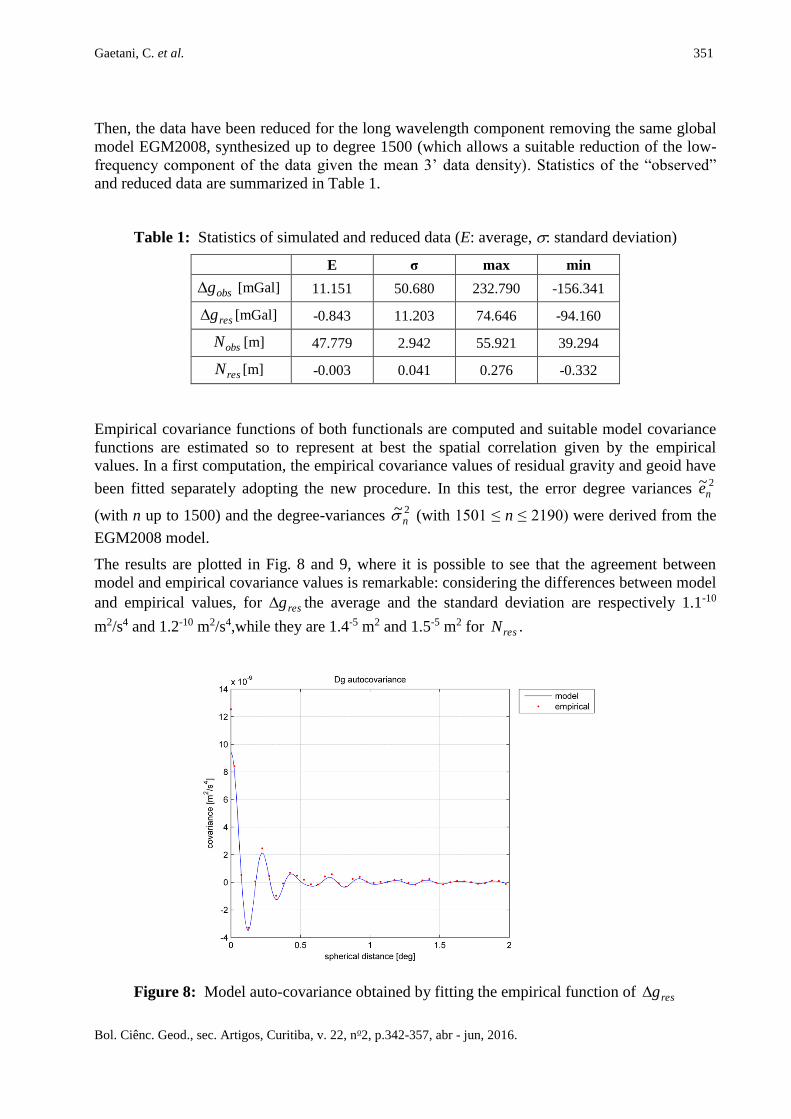
The results are plotted in Fig. 8 and 9, where it is possible to see that the agreement between

model and empirical covariance values is remarkable: considering the differences between model

and empirical values, for resg the average and the standard deviation are respectively 1.1-10

m2/s4 and 1.2-10 m2/s4,while they are 1.4-5 m2 and 1.5-5 m2 for resN .

Figure 8: Model auto-covariance obtained by fitting the empirical function of resg



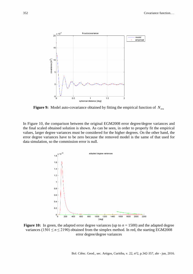
Figure 9: Model auto-covariance obtained by fitting the empirical function of resN

In Figure 10, the comparison between the original EGM2008 error degree/degree variances and

the final scaled obtained solution is shown. As can be seen, in order to properly fit the empirical

values, larger degree variances must be considered for the higher degrees. On the other hand, the

error degree variances have to be zero because the removed model is the same of that used for

data simulation, so the commission error is null.

Figure 10: In green, the adapted error degree variances (up to n = 1500) and the adapted degree

variances (1501 ≤ n ≤ 2190) obtained from the simplex method. In red, the starting EGM2008

error degree/degree variances



Moreover, with the proposed method it is possible to estimate the optimal solution considering

simultaneously both the functionals. The simplex method has been then applied to both empirical

covariances in order to get a set of scaled error degree/degree variances allowing a common

improved fit. Thus, both empirical auto-covariances of residual undulation and residual gravity

anomalies have been considered in the fitting procedure. The results are nearly identical to those

previously obtained. By using the estimated parameters in the model covariances one can also

define the model cross-covariance between resg and resN . The differences between this cross-

covariance model and the empirical cross-covariance values have average -3.6-8 m2/s2 and

standard deviation 5.6-7 m2/s2 (see Figure 11). Thus, despite the fact that the empirical cross-

covariance values were not included in the fitting procedure, the obtained cross-covariance

model properly interpolates the corresponding empirical function proving the numerical stability

of the devised method1.

Figure 11: The empirical cross-covariance emp

resNresgC and the model cross-covariance

resNresgC obtained by simultaneously fitting the empirical covariance functions of resN and

resg

In the same points where simulated data were generated, real observations of free-air gravity

anomalies have been then considered. The simplex method has been applied to them in order to

check for the new approach with real data too.

The adopted procedure is the classical remove technique (Forsberg, 1994). The free-air

anomalies have been reduced for the long wavelength component in the same way of the

simulated data, i.e. removing the global model EGM2008 up to degree 1500, while for the short

wavelengths the residual terrain correction (RTC) has been performed considering the detailed

DTM (pixel size: 3”3”) already used for evaluating the Italian geoid model Italgeo05 (Barzaghi

et al, 2007; Borghi et al., 2007). The reference altimetry grid for the RTC computation has been

1 However, it must be underlined that the procedure can be run also considering the empirical

cross-covariance values.



obtained filtering the DTM with a moving average window sized 5’5’. The size of the moving

window has been chosen according to the statistical properties of the residuals (minimization of

their root mean squared error). The RTC, both for gravity and height anomaly, has been

evaluated up to 120 km from each computation point. The program used in this computation is

TC from the GRAVSOFT package (Tscherning, 2004). Statistics of the observed and reduced

data are summarized in Table 2.

Table 2: Statistics of observed and reduced free-air gravity anomalies

E σ max min

obsg [mGal] 0.105 47.618 212.511 -162.22

resg [mGal] -0.236 9.210 94.649 -97.310

Then the simplex method has been applied to them. Again, as done in the simulations, the error

degree variances 2~

ne (with n up to 1500) and the degree-variances 2~n (with 1501 ≤ n ≤ 2190)

have been derived from the EGM2008 model.

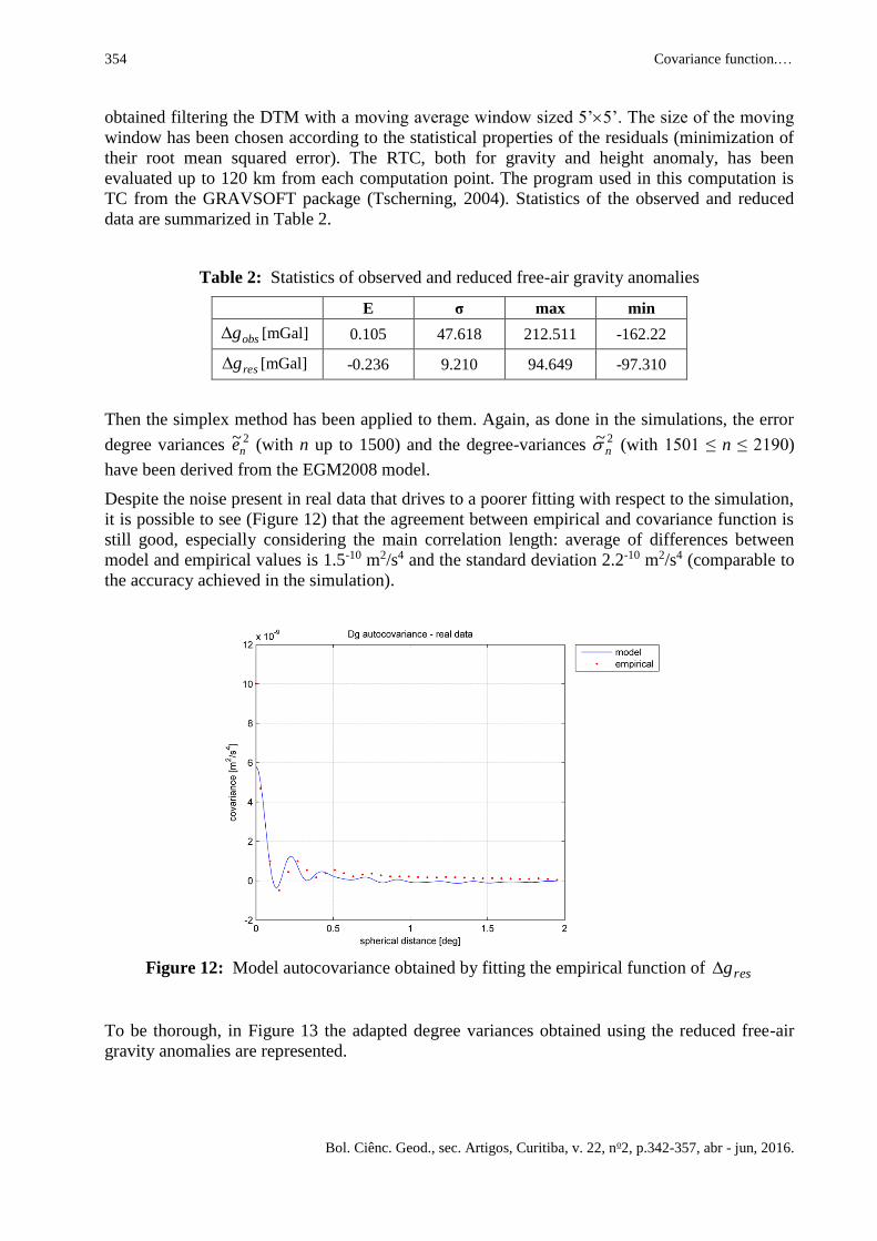
Despite the noise present in real data that drives to a poorer fitting with respect to the simulation,

it is possible to see (Figure 12) that the agreement between empirical and covariance function is

still good, especially considering the main correlation length: average of differences between

model and empirical values is 1.5-10 m2/s4 and the standard deviation 2.2-10 m2/s4 (comparable to

the accuracy achieved in the simulation).

Figure 12: Model autocovariance obtained by fitting the empirical function of resg

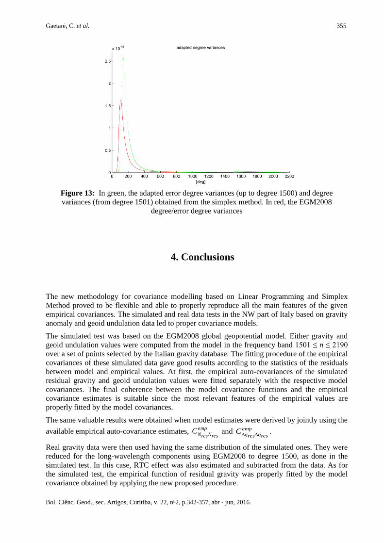
To be thorough, in Figure 13 the adapted degree variances obtained using the reduced free-air

gravity anomalies are represented.



Figure 13: In green, the adapted error degree variances (up to degree 1500) and degree

variances (from degree 1501) obtained from the simplex method. In red, the EGM2008

degree/error degree variances

4. Conclusions

The new methodology for covariance modelling based on Linear Programming and Simplex

Method proved to be flexible and able to properly reproduce all the main features of the given

empirical covariances. The simulated and real data tests in the NW part of Italy based on gravity

anomaly and geoid undulation data led to proper covariance models.

The simulated test was based on the EGM2008 global geopotential model. Either gravity and

geoid undulation values were computed from the model in the frequency band 1501 ≤ n ≤ 2190

over a set of points selected by the Italian gravity database. The fitting procedure of the empirical

covariances of these simulated data gave good results according to the statistics of the residuals

between model and empirical values. At first, the empirical auto-covariances of the simulated

residual gravity and geoid undulation values were fitted separately with the respective model

covariances. The final coherence between the model covariance functions and the empirical

covariance estimates is suitable since the most relevant features of the empirical values are

properly fitted by the model covariances.

The same valuable results were obtained when model estimates were derived by jointly using the

available empirical auto-covariance estimates, emp

resNresNC and emp

resgresgC

.

Real gravity data were then used having the same distribution of the simulated ones. They were

reduced for the long-wavelength components using EGM2008 to degree 1500, as done in the

simulated test. In this case, RTC effect was also estimated and subtracted from the data. As for

the simulated test, the empirical function of residual gravity was properly fitted by the model

covariance obtained by applying the new proposed procedure.



Thus, the new method for covariance fitting based on Linear Programming and Simplex Method

is effective and gives estimated model covariances which allow a suitable fitting to the empirical

values. Therefore, this procedure can be considered as a valuable tool in further developments

and applications of collocation.

REFERENCES

Barzaghi, Riccardo, Alessandra Borghi, Daniela Carrion, and Giovanna Sona. “Refining the

estimate of the Italian quasi-geoid.” Bollettino di Geodesia e Scienze Affini, 66, 3, (2007): 145-

160.

Barzaghi, Riccardo, Nikolaos Tselfes, Ilias N. Tziavos, and George S. Vergos. “Geoid and high-

resolution sea surface topography modelling in the Mediterranean from gravimetry, altimetry

and GOCE data: evaluation by simulation.” Journal of Geodesy, 83, 8 (2009): 751-772.

Borghi, Alessandra, Daniela Carrion, and Giovanna Sona. “Validation and fusion of different

databases in preparation of high-resolution geoid determination.” Geophysical Journal

International, 171,2 (2007): 539-549.

Chvatal, Vaclav. Linear Programming. San Francisco and London: W. H. Freeman, 1983.

De Gaetani, Carlo I. “Covariance models for geodetic applications of collocation.” PhD thesis,

Politecnico di Milano, 2012.

Forsberg, Rene. “Terrain effect in geoid computations.” In International School of the

Determination and Use of the Geoid Lecture Notes, Milano: IGeS, 1994: 159-181.

Ficken, Frederick A. The simplex method of linear programming. New York: Holt, Rinehart and

Winston, 1961.

Heiskanen, Weikko A., and Helmut Moritz. Physical Geodesy. San Francisco: W. H. Freeman,

1967.

Kaula, William M. Theory of satellite geodesy. New York: Dover, 2000.

Knudsen, Per. “Estimation and modelling of the local empirical covariance function using

gravity and satellite altimeter data.” Bulletin Geodesique, 61, 2 (1987): 145-160.

Moritz, Helmut. Advanced Physical Geodesy. Karlsruhe: Wichmann, 1980.

Mussio, Luigi. “Il metodo della collocazione minimi quadrati e le sue applicazioni per l’analisi

statistica dei risultati delle compensazioni.” In Ricerche di Geodesia Topografia e

Fotogrammetria, 4, Milano: CLUP, 1984: 305-338.

Pavlis, Nikolaos K., Simon A. Holmes, Steve C. Kenyon, and John K. Factor. “The development

and evaluation of the Earth Gravitational Model 2008 (EGM2008).” Journal of Geophysical

Research, 117 (2012): B04406(1-38).

Press, William H., Brian P. Flannery, Saul A. Teukolsky, William T. Vetterling. Numerical

Recipes: The Art of Scientific Computing. Cambridge University Press, 1989.

Sansò, Fernando. “Observables of Physical Geodesy and Their Analytical Representation.” In:

Geoid Determination, Theory and Methods, Sansò and Sideris Eds, Heidelberg: Springer, 2013a:

73-110.



Sansò, Fernando. “The Local Modelling of the Gravity Field by Collocation.” In: Geoid

Determination, Theory and Methods, Sansò and Sideris Eds, Heidelberg: Springer, 2013b: 203-

258.

Tscherning, Carl C., and Richard H. Rapp. “Closed Covariance Expressions for Gravity

Anomalies, Geoid Undulations, and Deflections of the Vertical Implied by Anomaly Degree-

Variance Models.” Reports of the Department of Geodetic Science, 208, The Ohio State

University, 1974.

Tscherning, Carl C. “Geoid determination by 3D least squares collocation.” In International

School of the Determination and Use of the Geoid Lecture Notes, Milano: IGeS, 2008: 193-210.

Tselfes, Nikolaos. “Global and local geoid modelling with GOCE data and collocation.” PhD

thesis, Politecnico di Milano, 2008.

Submetido em Setembro de 2015.

Aceito em Setembro de 2015.

Documents

COVARIANCE FUNCTION MODELLING IN LOCAL GEODETIC … · using the Simplex Method. The procedure has been implemented in a FORTRAN95 software The procedure has been implemented in a