Embed Size (px)
Citation preview

arX
iv:a
stro
-ph/
0402
060
v1
3 Fe
b 20
04
Covariant Linear Perturbation Formalism
Wayne Hu∗
CfCP, Department of Astronomy and Astrophysics, University of Chicago
Lecture given at the:
ICTP Summer School on Astroparticle Physics and Cosmology
Trieste, June 17-July 5, 2002
LNS

Abstract
Lecture notes on covariant linear perturbation theory and its applications to inflation, darkenergy or matter and the cosmic microwave background.
Keywords:
PACS numbers:

Contents
1 Apologia 5
2 Formalism 5
2.1 Covariant Approach . . . . . . . . . . . . . . . . . . . . . . . . . . . . . . . . . . . . 5
2.2 Metric Representation . . . . . . . . . . . . . . . . . . . . . . . . . . . . . . . . . . . 5
2.3 Matter Representation . . . . . . . . . . . . . . . . . . . . . . . . . . . . . . . . . . . 6
2.4 Closure . . . . . . . . . . . . . . . . . . . . . . . . . . . . . . . . . . . . . . . . . . . 6
2.5 Friedmann Equations . . . . . . . . . . . . . . . . . . . . . . . . . . . . . . . . . . . . 7
2.6 Linearization and Eigenmodes . . . . . . . . . . . . . . . . . . . . . . . . . . . . . . . 8
2.7 Covariant Scalar Equations . . . . . . . . . . . . . . . . . . . . . . . . . . . . . . . . 9
2.8 Covariant Vector Equations . . . . . . . . . . . . . . . . . . . . . . . . . . . . . . . . 9
2.9 Covariant Tensor Equations . . . . . . . . . . . . . . . . . . . . . . . . . . . . . . . . 10
2.10 Multicomponent universe . . . . . . . . . . . . . . . . . . . . . . . . . . . . . . . . . 11
3 Gauge 11
3.1 Semantics . . . . . . . . . . . . . . . . . . . . . . . . . . . . . . . . . . . . . . . . . . 11
3.2 Gauge Transformation . . . . . . . . . . . . . . . . . . . . . . . . . . . . . . . . . . . 12
3.3 Newtonian Gauge . . . . . . . . . . . . . . . . . . . . . . . . . . . . . . . . . . . . . . 13
3.4 Comoving Gauge . . . . . . . . . . . . . . . . . . . . . . . . . . . . . . . . . . . . . . 13
3.5 Synchronous Gauge . . . . . . . . . . . . . . . . . . . . . . . . . . . . . . . . . . . . . 15
3.6 Spatially Flat Gauge: . . . . . . . . . . . . . . . . . . . . . . . . . . . . . . . . . . . . 16
3.7 Uniform Density Gauge: . . . . . . . . . . . . . . . . . . . . . . . . . . . . . . . . . . 16
4 Inflationary Perturbations 17
4.1 Horizon, Flatness, Relics Redux . . . . . . . . . . . . . . . . . . . . . . . . . . . . . . 17
4.2 Scalar Fields . . . . . . . . . . . . . . . . . . . . . . . . . . . . . . . . . . . . . . . . 18
4.3 Gauge Choice . . . . . . . . . . . . . . . . . . . . . . . . . . . . . . . . . . . . . . . . 18
4.4 Perturbation Evolution . . . . . . . . . . . . . . . . . . . . . . . . . . . . . . . . . . . 19
4.5 Slow Roll Limit . . . . . . . . . . . . . . . . . . . . . . . . . . . . . . . . . . . . . . . 21
4.6 Quantum Fluctuations . . . . . . . . . . . . . . . . . . . . . . . . . . . . . . . . . . . 22
4.7 Gravitational Waves . . . . . . . . . . . . . . . . . . . . . . . . . . . . . . . . . . . . 22
5 Dark Matter and Energy 23
5.1 Degrees of Freedom . . . . . . . . . . . . . . . . . . . . . . . . . . . . . . . . . . . . . 23
5.2 Generalized Equations of State . . . . . . . . . . . . . . . . . . . . . . . . . . . . . . 23
5.3 Examples . . . . . . . . . . . . . . . . . . . . . . . . . . . . . . . . . . . . . . . . . . 24
5.4 Initial Conditions . . . . . . . . . . . . . . . . . . . . . . . . . . . . . . . . . . . . . . 25
6 Cosmic Microwave Background 26
6.1 Boltzmann Equation . . . . . . . . . . . . . . . . . . . . . . . . . . . . . . . . . . . . 26
6.2 Eigenmodes . . . . . . . . . . . . . . . . . . . . . . . . . . . . . . . . . . . . . . . . . 27
6.3 Collision Term . . . . . . . . . . . . . . . . . . . . . . . . . . . . . . . . . . . . . . . 29
6.4 Temperature-Polarization Hierarchy . . . . . . . . . . . . . . . . . . . . . . . . . . . 31
6.5 Integral Solution . . . . . . . . . . . . . . . . . . . . . . . . . . . . . . . . . . . . . . 31
6.6 Power Spectra . . . . . . . . . . . . . . . . . . . . . . . . . . . . . . . . . . . . . . . . 32

4 Perturbation Theory
7 Epilogue 32
8 Acknowledgments 32
References 33

5
1 Apologia
In these informal Lecture Notes on formalism, I gather together a few elements of covariant linear
perturbation theory and its applications to inflation, dark energy or matter and the cosmic mi-
crowave background (CMB). I make no attempt to cite properly the original source material. My
usual, lame defense is “it’s all in Bardeen’s paper [1]” – go read it and ignore these lecture notes!
Seriously though, in addition to [1], I have heavily relied on a few sources in compiling the
various sections and refer the reader to references therein. The covariant formalism presented in §2and gauge transformation material in §3 draws from [2] distilled in [3]. Applications to inflation in
§4 draw from [4], to dark energy and matter in §5 from [5], and to the CMB in §6 from [6]. For the
last topic, despite great recent progress on the phenomenology, I have limited myself to the formal
aspects that relate to covariant perturbation theory. My defense here is “everything that doesn’t
go out of date as soon as it’s written is in Peebles & Yu [7]” – go read it and stop looking for CMB
reviews! My other defense is Matias Zaldarriaga was supposed to cover that in this School so blame
him! As for the equation density and opaqueness of these Lecture Notes, I have no excuse – take
it as an homage to the Dick Bond lectures of my own student days – at least there are no figures
with 100 curves. As Martin White would say, you are physicists; you don’t need figures!
2 Formalism
2.1 Covariant Approach
Perturbation theory proceeds by linearizing the Einstein equations
Gµν = 8πGTµν , (1)
around a background metric. Here Gµν is the Einstein tensor and Tµν is the stress energy tensor.
The Bianchi identity ∇µGµν = 0 guarantees the covariant conservation of the total stress-energy
∇µTµν = 0 . (2)
The conservation equation is redundant with the Einstein equation but is a particularly useful rep-
resentation of the equations when there are multiple components to the matter that are separately
conserved.
Let us begin by distinguishing between covariant equations and invariant variables:
Covariant = equations takes same form in all coordinate systems
Invariant = variable takes the same value in all coordinate systems
In an evolving universe, the meaning of a density perturbation necessarily requires the specification
of the time slicing in relation to the background and hence there is no such thing as a gauge
or coordinate invariant density perturbation. Likewise for elements of the metric. The general
covariance of the Einstein and conservation equations, on the other hand, can be preserved. With
covariant equations one can, after the fact of their derivation, choose the gauge that best suits a
given physical problem, e.g. the evolution of inflationary, dark energy, or CMB fluctuations.
2.2 Metric Representation
Let us take the background metric to be the general homogeneous and isotropic, or Friedmann-
Robertson-Walker form. Here the degrees of freedom are the (comoving) spatial curvature K and
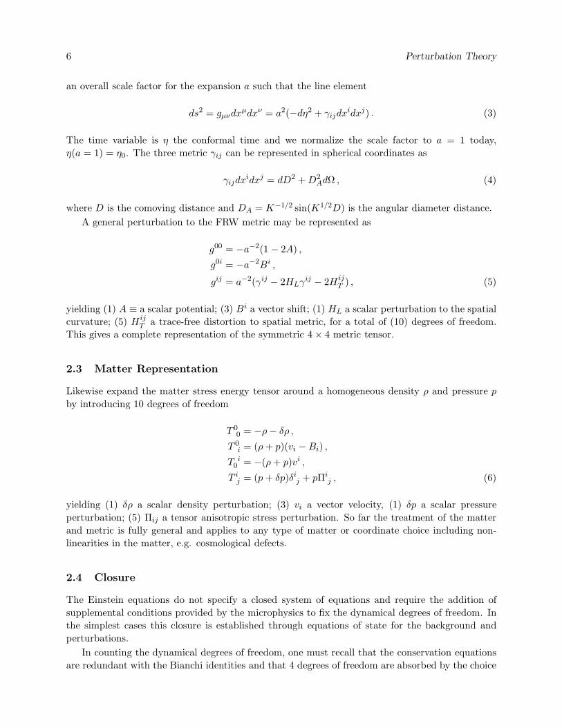
6 Perturbation Theory
an overall scale factor for the expansion a such that the line element
ds2 = gµνdxµdxν = a2(−dη2 + γijdx
idxj) . (3)
The time variable is η the conformal time and we normalize the scale factor to a = 1 today,
η(a = 1) = η0. The three metric γij can be represented in spherical coordinates as
γijdxidxj = dD2 +D2
AdΩ , (4)
where D is the comoving distance and DA = K−1/2 sin(K1/2D) is the angular diameter distance.
A general perturbation to the FRW metric may be represented as
g00 = −a−2(1 − 2A) ,
g0i = −a−2Bi ,
gij = a−2(γij − 2HLγij − 2H ij
T ) , (5)
yielding (1) A ≡ a scalar potential; (3) Bi a vector shift; (1) HL a scalar perturbation to the spatial
curvature; (5) H ijT a trace-free distortion to spatial metric, for a total of (10) degrees of freedom.
This gives a complete representation of the symmetric 4 × 4 metric tensor.
2.3 Matter Representation
Likewise expand the matter stress energy tensor around a homogeneous density ρ and pressure p
by introducing 10 degrees of freedom
T 00 = −ρ− δρ ,
T 0i = (ρ+ p)(vi −Bi) ,
T i0 = −(ρ+ p)vi ,
T ij = (p + δp)δij + pΠij , (6)
yielding (1) δρ a scalar density perturbation; (3) vi a vector velocity, (1) δp a scalar pressure
perturbation; (5) Πij a tensor anisotropic stress perturbation. So far the treatment of the matter
and metric is fully general and applies to any type of matter or coordinate choice including non-
linearities in the matter, e.g. cosmological defects.
2.4 Closure
The Einstein equations do not specify a closed system of equations and require the addition of
supplemental conditions provided by the microphysics to fix the dynamical degrees of freedom. In
the simplest cases this closure is established through equations of state for the background and
perturbations.
In counting the dynamical degrees of freedom, one must recall that the conservation equations
are redundant with the Bianchi identities and that 4 degrees of freedom are absorbed by the choice

7
of coordinate system
20 Variables (10 metric; 10 matter)
−10 Einstein equations
−4 Conservation equations
+4 Bianchi identities
−4 Gauge (coordinate choice 1 time, 3 space)
——
6 Degrees of freedom
Without loss of generality these six dynamical degrees of freedom can be taken to be the 6 compo-
nents of the matter stress tensor.
Since the background is isotropic, the unperturbed matter is described entirely by the pressure
p(a) or equivalently w(a) ≡ p(a)/ρ(a), the equation of state parameter. For the perturbations
specification of the relationship between δp, Π and the other perturbations, e.g. δρ and v suffices.
2.5 Friedmann Equations
The unperturbed Einstein equation yields the ordinary Friedmann equation which relates the ex-
pansion rate to the energy density(
a
a
)2
+K =8πG
3a2ρ , (7)
where overdots represent conformal time derivatives, and the acceleration Friedmann equation
which relates the change in the expansion rate to the equation of state
d
dη
(
a
a
)
= −4πG
3a2(ρ+ 3p) , (8)
so that w ≡ p/ρ < −1/3 implies acceleration of the expansion.
The conservation law ∇µTµν = 0 implies
ρ
ρ= −3(1 +w)
a
a, (9)
which by virtue of the Bianchi identity can be derived from the Friedmann equation.
The counting exercise for the background becomes
20 Variables (10 metric; 10 matter)
−17 Homogeneity and Isotropy
−2 Einstein equations
−1 Conservation equations
+1 Bianchi identities
——
1 Degree of freedom
Without loss of generality this degree of freedom can be chosen to be the equation of state w(a) =
p(a)/ρ(a).

8 Perturbation Theory
2.6 Linearization and Eigenmodes
For the inhomogenous universe, the Einstein tensor Gµν is in general constructed out of a nonlinear
combination of metric fluctuations. Metric fluctuations typically remain small even in the presence
of larger matter fluctuations. Hence we linearize the left hand side of the Einstein equations to
obtain a set of partial differential equations that are linear in the variables.
These equations may then be decoupled into a set of ordinary differential equations by employing
normal modes under translation and rotation. The scalar, vector and tensor eigenmodes of the
Laplacian operator form a complete set
∇2Q(0) = −k2Q(0) S ,
∇2Q(±1)i = −k2Q
(±1)i V ,
∇2Q(±2)ij = −k2Q
(±2)ij T .
(10)
In a spatially flat (K = 0) universe, the eigenmodes are essentially plane waves
Q(0) = exp(ik · x) ,
Q(±1)i =
−i√2(e1 ± ie2)i exp(ik · x) ,
Q(±2)ij = −
√
3
8(e1 ± ie2)i(e1 ± ie2)j exp(ik · x) , (11)
where e1, e2 are unit vectors spanning the plane transverse to k.
Vector modes represent divergence-free vectors (vorticity); tensor modes represent transverse
traceless tensors (gravitational waves)
∇iQ(±1)i = 0 , ∇iQ
(±2)ij = 0 , γijQ
(±2)ij = 0 . (12)
Curl free vectors and the longitudinal components of tensors are represented with covariant deriva-
tives of the scalar and vector modes
Q(0)i = −k−1∇iQ
(0) ,
Q(0)ij = (k−2∇i∇j +
1
3γij)Q
(0) ,
Q(±1)ij = − 1
2k[∇iQ
(±1)j + ∇jQ
(±1)i ] , (13)
For the kth eigenmode, the scalar components become
A(x) = A(k)Q(0) , HL(x) = HL(k)Q(0) ,
δρ(x) = δρ(k)Q(0) , δp(x) = δp(k)Q(0) ,(14)
the vectors components become
Bi(x) =
1∑
m=−1
B(m)(k)Q(m)i , vi(x) =
1∑
m=−1
v(m)(k)Q(m)i , (15)
and the tensors components become
HT ij(x) =2
∑
m=−2
H(m)T (k)Q
(m)ij , Πij(x) =
2∑
m=−2
Π(m)(k)Q(m)ij . (16)
An arbitrary set of spatial perturbations can be formed through a superposition of the eigenmodes
given their completeness.

9
2.7 Covariant Scalar Equations
The Einstein equations for the scalar modes (suppressing 0 superscripts) become
(k2 − 3K)[HL +1
3HT +
a
a(B
k− HT
k2)] = 4πGa2
[
δρ+ 3a
a(ρ+ p)
v −B
k
]
,
k2(A+HL +1
3HT ) +
(
d
dη+ 2
a
a
)
(kB − HT ) = −8πGa2pΠ ,
a
aA− HL − 1
3HT − K
k2(kB − HT ) = 4πGa2(ρ+ p)
v −B
k,
[
2a
a− 2
(
a
a
)2
+a
a
d
dη− k2
3
]
A−[
d
dη+a
a
]
(HL +kB
3) = 4πGa2(δp +
1
3δρ) . (17)
The conservation equations become the continuity and Navier-Stokes equations[
d
dη+ 3
a
a
]
δρ+ 3a
aδp = −(ρ+ p)(kv + 3HL) , (18)
[
d
dη+ 4
a
a
]
(ρ+ p)v −B
k= δp − 2
3(1 − 3
K
k2)pΠ + (ρ+ p)A . (19)
In the absence of anisotropic stress, the Navier-Stokes equation is known as the Euler equation.
These equations are not independent due to the Bianchi identity. For numerical solutions it
suffices to retain 2 Einstein equations and the 2 conservation laws. The counting exercise becomes
8 Variables (4 metric; 4 matter)
−4 Einstein equations
−2 Conservation equations
+2 Bianchi identities
−2 Gauge (coordinate choice 1 time, 1 space)
——
2 Degrees of freedom
Without loss of generality we may choose the dynamical components to be those of the stress
tensor δp, Π. Microphysics defines their relationship to the density and velocity perturbations. In
fluid dynamics this is the familiar need of a prescription for viscosity and heat conduction (entropy
generation) to close the system of equations.
2.8 Covariant Vector Equations
The vector Einstein equations become
(1 − 2K
k2)(kB(±1) − H
(±1)T ) = 16πGa2(ρ+ p)
v(±1) −B(±1)
k,
[
d
dη+ 2
a
a
]
(kB(±1) − H(±1)T ) = −8πGa2pΠ(±1) , (20)
and the conservation equations become[
d
dη+ 4
a
a
]
(ρ+ p)v(±1) −B(±1)
k= −1
2(1 − 2
K
k2)pΠ(±1) . (21)

10 Perturbation Theory
Since gravity provides no source to vorticity, any initial vector perturbation will simply decay unless
vector anisotropic stresses are continuously generated in the matter. In the absence of nonlinearities
in the matter, e.g. from cosmological defects, vector perturbations can generally be ignored.
The counting exercise for vectors becomes
8 Variables (4 metric; 4 matter)
−4 Einstein equations
−2 Conservation equations
+2 Bianchi identities
−2 Gauge (coordinate choice 2 space))
——
2 Degrees of freedom
Without loss of generality, we can choose these to be the vector components of the stress tensor
Π(±1).
2.9 Covariant Tensor Equations
The Einstein equation for the tensor modes is
[
d2
dη2+ 2
a
a
d
dη+ (k2 + 2K)
]
H(±2)T = 8πGa2pΠ(±2) , (22)
and the counting exercise becomes
4 Variables (2 metric; 2 matter)
−2 Einstein equations
−0 Conservation equations
+0 Bianchi identities
−0 Gauge (coordinate choice 1 time, 1 space)
——
2 Degrees of freedom
without loss of generality we can choose these to be represented by the tensor components of the
stress tensor Π(±2).
In the absence of anisotropic stresses and spatial curvature, the tensor equation becomes a
simple source-free gravitational wave propagation equation
H(±2)T + 2
a
aH
(±2)T + k2H
(±2)T = 0 , (23)
which has solutions
H(±2)T (kη) = C1H1(kη) + C2H2(kη) , (24)
H1(x) ∝ x−mjm(x) ,
H2(x) ∝ x−mnm(x) ,

11
where m = (1 − 3w)/(1 + 3w). If w > −1/3 then the gravitational wave amplitude is constant
above horizon x ≪ 1 and then oscillates and damps. If w < −1/3 then gravity wave oscillates
and freezes into some value. It will be useful to recall these solutions when considering the Klein
Gordon equation for scalar field fluctuations during inflation and dark energy domination.
2.10 Multicomponent universe
With multiple matter components, the Einstein equations of course remain valid but with the
associations
δρ =∑
J
δρJ ,
(ρ+ p)v(m) =∑
J
(ρJ + pJ)v(m)J ,
pΠ(m) =∑
J
pJΠ(m)J , (25)
where J indexes the different components, e.g. photons, baryons, neutrinos, dark matter, dark
energy, inflaton, cosmological defects. The conservation equations remain valid for each non-
interacting subsystem. Interactions can be represented as non-ideality in the specification of the
stress degrees of freedom (e.g. viscous and entropic terms) in each subsystem or by explicitly
writing down energy and momentum exchange terms in separate conservation equations (see e.g.
§6).
3 Gauge
3.1 Semantics
The covariant equations of the last section hold true under any coordinate choice for the relation-
ship between the unperturbed FRW background and the perturbations. Choice of a particular
relationship, called a gauge choice can help simplify the equations for the physical conditions at
hand. The price to pay is that the perturbation variables are quantities that take on the meaning
of say a density perturbation or a spatial curvature perturbation only on a specific gauge – but
that is in any case unavoidable.
Since the preferred gauge for simplifying the physics can change as the universe evolves, it
is often useful to access the perturbation variables of one gauge from those of another gauge.
This operation proceeds by writing down a covariant form for gauge specific variables through
the properties of gauge transformation. It is the analogue of deriving covariant equations for the
dynamics but for the perturbation variables themselves. Since these gauge specific variables are
now thought of in a coordinate independent way, this procedure is called in the literature endowing
a variable with a “gauge invariant” meaning. Note neither the numerical values nor the physical
interpretation of the variables has changed. “Gauge invariance“ here is an operational distinction
that indicates a freedom to calculate gauge specific quantities from an arbitrary gauge. Perturbation
variables still only take on their given meaning in the given gauge. Under this definition of gauge
invariance, the perturbation variables of any fully specified gauge is gauge invariant. We will
hereafter avoid using this terminology.
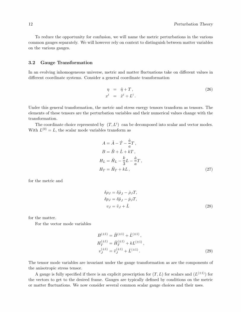
12 Perturbation Theory
To reduce the opportunity for confusion, we will name the metric perturbations in the various
common gauges separately. We will however rely on context to distinguish between matter variables
on the various gauges.
3.2 Gauge Transformation
In an evolving inhomogeneous universe, metric and matter fluctuations take on different values in
different coordinate systems. Consider a general coordinate transformation
η = η + T , (26)
xi = xi + Li .
Under this general transformation, the metric and stress energy tensors transform as tensors. The
elements of these tensors are the perturbation variables and their numerical values change with the
transformation.
The coordinate choice represented by (T,Li) can be decomposed into scalar and vector modes.
With L(0) = L, the scalar mode variables transform as
A = A− T − a
aT ,
B = B + L+ kT ,
HL = HL − k
3L− a
aT ,
HT = HT + kL , (27)
for the metric and
δρJ = δρJ − ρJT,
δpJ = δpJ − pJT,
vJ = vJ + L (28)
for the matter.
For the vector mode variables
B(±1) = B(±1) + L(±1) ,
H(±1)T = H
(±1)T + kL(±1) ,
v(±1)J = v
(±1)J + L(±1) . (29)
The tensor mode variables are invariant under the gauge transformation as are the components of
the anisotropic stress tensor.
A gauge is fully specified if there is an explicit prescription for (T,L) for scalars and (L(±1)) for
the vectors to get to the desired frame. Gauges are typically defined by conditions on the metric
or matter fluctuations. We now consider several common scalar gauge choices and their uses.

13
3.3 Newtonian Gauge
The Newtonian or longitudinal gauge is defined by diagonal metric fluctuations
B = HT = 0 ,
Ψ ≡ A (Newtonian potential) ,
Φ ≡ HL (Newtonian curvature) , (30)
where Ψ plays the role of the gravitational potential in the Newtonian approximation and Φ is
the Newtonian spatial curvature. This condition completely fixes the gauge by giving explicit
expressions for the gauge transformation
L = −HT
k,
T = −Bk
+1
k2
d
dηHT . (31)
The Einstein equations become
(k2 − 3K)Φ = 4πGa2
[
δρ+ 3a
a(ρ+ p)
v
k
]
,
k2(Ψ + Φ) = −8πGa2pΠ . (32)
Note that for scales inside the Hubble length k(a/a)−1 ≫ 1, the first equation becomes the Poisson
equation for the perturbations and if the anisotropic stress of the matter is much less than the
energy density perturbation (as in the case of non-relativistic matter), Ψ ≈ −Φ.
The conservation laws for the Jth non-interacting subsystem becomes[
d
dη+ 3
a
a
]
δρJ + 3a
aδpJ = −(ρJ + pJ)(kvJ + 3Φ) , (33)
[
d
dη+ 4
a
a
]
(ρJ + pJ)vJk
= δpJ − 2
3(1 − 3
K
k2)pJΠJ + (ρJ + pJ)Ψ . (34)
Aside from the Φ term, these are the usual relativistic fluid equations. Since Φ represents a
perturbation to the scale factor, Φ represents the perturbation to the redshifting of the density in
an expanding universe [see Eqn. (9)].
The Newtonian gauge is useful since it most closely corresponds to Newtonian gravity. A
drawback is that as k(a/a)−1 → 0 there are relativistic corrections to the Poisson equation which
make a straightforward implementation of the equations numerically unstable. Likewise in this
limit, the metric effects on density though Φ muddle the interpretation of the conservation law.
3.4 Comoving Gauge
The comoving gauge is defined by
B = v (T 0i = 0) ,
HT = 0 ,
ξ = A ,
ζ = HL (comoving curvature) , (35)

14 Perturbation Theory
which completely fixes the gauge through
T = (v − B)/k ,
L = −HT/k . (36)
The Einstein equations become
ζ +Kv/k − a
aξ = 0 ,
v + 2a
av + k(ζ + ξ) = −8πGa2pΠ , (37)
and the conservation laws become[
d
dη+ 3
a
a
]
δρJ + 3a
aδpJ = −(ρJ + pJ)(kvJ + 3ζ) , (38)
[
d
dη+ 4
a
a
]
(ρJ + pJ)vJ − v
k= δpJ − 2
3(1 − 3
K
k2)pJΠJ + (ρJ + pJ)ξ . (39)
In particular the Navier-Stokes equation for the total matter becomes an algebraic relation between
total stress fluctuations and the potential
(ρ+ p)ξ = −δp+2
3
(
1 − 3K
k
)
pΠ (40)
so that these equations are a complete set.
Eliminating ξ allows us to write a conservation law for the comoving curvature
ζ +Kv/k =a
a
[
− δp
ρ+ p+
2
3
(
1 − 3K
k2
)
p
ρ+ pΠ
]
. (41)
On scales well below the curvature scale, this equation states that the comoving curvature only
changes in response to stress gradients which move matter around. This statement corresponds to
the non-relativistic intuition that causality should prohibit evolution above the horizon scale. This
conservation law is the fundamental virtue of the comoving gauge. An auxiliary consideration is
that the comoving gauge variables are numerically stable.
From an alternate gauge choice, one can construct the Newtonian variables via the gauge
transformation relation
ζ = HL +1
3HT − a
a
v − B
k. (42)
For example, since in the Newtonian gauge HT and v take on the same values
Φ = ζ +a
a
v
k
= ζ +2
3
1
1 + w
1
1 +K(a/a)−2[Ψ − Φ/(a/a)] . (43)
If the curvature is negligible, stress perturbations are negligible, and the equation of state w is
constant
Φ =3 + 3w
5 + 3wζ , (44)
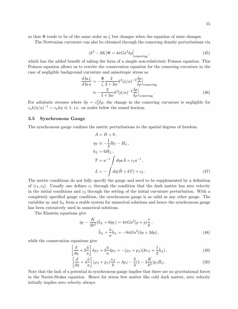
15
so that Φ tends to be of the same order as ζ but changes when the equation of state changes.
The Newtonian curvature can also be obtained through the comoving density perturbations via
(k2 − 3K)Φ = 4πGa2δρ∣
∣
∣
comoving, (45)
which has the added benefit of taking the form of a simple non-relativistic Poisson equation. This
Poisson equation allows us to rewrite the conservation equation for the comoving curvature in the
case of negligible background curvature and anisotropic stress as
d ln ζ
d ln a= −Φ
ζ
2
3 + 3wk2(a/a)−2 δp
δρ
∣
∣
∣
comoving
≈ − 2
5 + 3wk2(a/a)−2 δp
δρ
∣
∣
∣
comoving. (46)
For adiabatic stresses where δp = c2aδρ, the change in the comoving curvature is negligible for
cak(a/a)−1 ∼ cakη ≪ 1, i.e. on scales below the sound horizon.
3.5 Synchronous Gauge
The synchronous gauge confines the metric perturbations to the spatial degrees of freedom
A = B = 0 ,
ηT ≡ −1
3HT −HL ,
hL = 6HL ,
T = a−1
∫
dηaA+ c1a−1 ,
L = −∫
dη(B + kT ) + c2 . (47)
The metric conditions do not fully specify the gauge and need to be supplemented by a definition
of (c1, c2). Usually one defines c1 through the condition that the dark matter has zero velocity
in the initial conditions and c2 through the setting of the initial curvature perturbation. With a
completely specified gauge condition, the synchronous gauge is as valid as any other gauge. The
variables ηT and hL form a stable system for numerical solutions and hence the synchronous gauge
has been extensively used in numerical solutions.
The Einstein equations give
ηT − K
2k2(hL + 6ηT ) = 4πGa2(ρ+ p)
v
k,
hL +a
ahL = −8πGa2(δρ+ 3δp) , (48)
while the conservation equations give[
d
dη+ 3
a
a
]
δρJ + 3a
aδpJ = −(ρJ + pJ)(kvJ +
1
2hL) , (49)
[
d
dη+ 4
a
a
]
(ρJ + pJ)vJk
= δpJ − 2
3(1 − 3
K
k2)pJΠJ . (50)
Note that the lack of a potential in synchronous gauge implies that there are no gravitational forces
in the Navier-Stokes equation. Hence for stress free matter like cold dark matter, zero velocity
initially implies zero velocity always.

16 Perturbation Theory
3.6 Spatially Flat Gauge:
Conversely the spatially flat gauge eliminates spatial metric perturbations
HL = HT = 0 ,
αF ≡ A ,
βF ≡ B ,
T =
(
a
a
)−1 (
HL +1
3HT
)
.
L = −HT/k , (51)
The Einstein equations give
βF + 2a
aβF + kαF = −8πGa2pΠ/k ,
a
aαF − K
kβF = 4πGa2(ρ+ p)
v − βFk
, (52)
and the conservation equations give[
d
dη+ 3
a
a
]
δρJ + 3a
aδpJ = −(ρJ + pJ)kvJ , (53)
[
d
dη+ 4
a
a
]
(ρJ + pJ)vJ − βF
k= δpJ − 2
3(1 − 3
K
k2)pJΠJ + (ρJ + pJ)αF . (54)
The spatially flat gauge is useful in that it is the complement of the comoving gauge. In particular
the comoving curvature is constructed from Eqn. (42) as
ζ = − aa
v − βFk
. (55)
This gauge is most often used in inflationary calculations where v−βF is closely related to pertur-
bations in the inflaton field.
3.7 Uniform Density Gauge:
Finally, one can eliminate the density perturbation δρ = 0 with the choice
HT = 0 ,
ζδ ≡ HL
Bδ ≡ B
Aδ ≡ A
T =δρ
ρ
L = −HT /k (56)
The Einstein equations become
(k2 − 3K)[ζδ +a
a
Bδk
] = 12πGa2 a
a(ρ+ p)
v −Bδk
,
a
aAδ − ζc −
K
kBδ = 4πGa2(ρ+ p)
v −Bδk
, (57)

17
from which Aδ may be eliminated in favor of ζδ and Bδ. The conservation equations become
[
d
dη+ 3
a
a
]
δρJ + 3a
aδpJ = −(ρJ + pJ)(kvJ + 3ζδ) ,
[
d
dη+ 4
a
a
]
(ρJ + pJ)vJ −Bδ
k= δpJ − 2
3(1 − 3
K
k2)pJΠJ + (ρJ + pJ)Aδ . (58)
Notice that the continuity equation for the net density perturbation becomes a conservation law
ζδ = − aa
δp
ρ+ p− 1
3kv . (59)
Furthermore since δρ = 0, δp is the non-adiabatic stress [see Eqn. (46)] and the conservation law
resembles that of the comoving curvature [see Eqn. (41)]. More specifically, the two curvatures are
related by
ζδ = ζ +1
3
δρ
(ρ+ p)
∣
∣
∣
comoving. (60)
By the same argument as that following Eqn. (46), these two curvatures coincide outside the horizon
if the stresses are adiabatic. Hence they are often used interchangeably in the literature. It bears
an even simpler relationship to density fluctuations in the spatially flat gauge
ζδ =1
3
δρ
(ρ+ p)
∣
∣
∣
flat. (61)
For a single particle species δρ/(ρ + p) = δn/n, the number density fluctuation. These simple
relationships make ζδ and related variables useful for the consideration of relative number density
or isocurvature perturbations in a multicomponent system.
4 Inflationary Perturbations
4.1 Horizon, Flatness, Relics Redux
Inflation was originally proposed to solve the horizon, flatness and relic problem: that the cosmic
microwave background (CMB) temperature is isotropic across scales larger than Hubble length
at recombination; that the spatial curvature scale is at least comparable to the current Hubble
length; that the energy density is not dominated by defect relics from phase transitions in the early
universe.
Measurements of fluctuations in the CMB imply a stronger version of the problems. They
imply spatial curvature fluctuations above the Hubble length and rule out cosmological defects as
the primary source of structure in the universe, i.e. they are absent as a significant component of
the perturbations as well as the background. The conservation of the comoving curvature above
the comoving Hubble length (a/a)−1 ≪ 1 leaves a paradox as to their origin. As long as the Hubble
length monotonically increases, there will always be a time η ∼ k−1 before which ζ cannot have
been generated dynamically. For sufficiently small k, this time exceeds the recombination epoch at
a ∼ 10−3 where the CMB fluctuations are formed.
The comoving Hubble length decreases if ρ scales more slowly than a−2 or w < −1/3, i.e. if
the expansion accelerates [see Eqn. (7-8)]. Vacuum energy or a cosmological constant can provide
for acceleration but not for re-entry into the matter-radiation dominated expansion. On the other

18 Perturbation Theory
hand, a scalar field has both a potential and kinetic energy and provides a mechanism by which
acceleration can end. A major success of the inflationary model is that the same mechanism that
solves the horizon, flatness and relic problems by making the observed universe today much smaller
than the Hubble length at the beginning of inflation predicts super-Hubble curvature perturbations
from quantum fluctuations in the scalar field. The evolution of scalar field fluctuations can be
usefully described in the gauge covariant framework.
4.2 Scalar Fields
The covariant perturbation theory described in the previous sections also applies to the inflationary
universe. The stress-energy tensor of a scalar field rolling in the potential V (φ) is
T µν = ∇µϕ∇νϕ− 1
2(∇αϕ∇αϕ+ 2V )δµν . (62)
For the backround φ ≡ φ0 and
ρφ =1
2a−2φ2
0 + V , pφ =1
2a−2φ2
0 − V . (63)
If the scalar field is kinetic energy dominated wφ = pφ/ρφ → 1, whereas if it is potential energy
dominated wφ = pφ/ρφ → −1.
The equation of motion for the scalar field is simply the energy conservation equation
ρφ = −3(ρφ + pφ)a
a, (64)
re-written in terms of φ0 and V
φ0 + 2a
aφ0 + a2V ′ = 0 . (65)
Likewise for the perturbations φ = φ0 + φ1
δρφ = a−2(φ0φ1 − φ20A) + V ′φ1 ,
δpφ = a−2(φ0φ1 − φ20A) − V ′φ1 ,
(ρφ + pφ)(vφ −B) = a−2kφ0φ1 ,
pφπφ = 0 , (66)
the continuity equation implies
φ1 = −2a
aφ1 − (k2 + a2V ′′)φ1 + (A− 3HL − kB)φ0 − 2Aa2V ′ , (67)
while the Euler equation expresses an identity.
4.3 Gauge Choice
We are interested in inflation as a means of generating comoving curvature perturbations and so
naively it would seem that inflationary perturbations should be calculated in the comoving gauge.
However for a scalar field dominated universe, the comoving gauge sets B = v = vφ and hence
φ1 = 0. In the comoving gauge, the scalar field carries no perturbations by definition! This fact
will be useful for treating scalar fields as a dark energy candidate in the next section: in the absence

19
of scalar field fluctuations, energy density and pressure perturbations come purely from the kinetic
terms so that δpφ = δρφ yielding stable perturbations within the Hubble length.
The gauge covariant approach allows us to compute the comoving curvature from variables in
another gauge. Since a scalar field transforms as a scalar field
φ1 = φ1 − φ0T (68)
the comoving gauge is obtained from an arbitrary gauge by the time slicing change T = φ1/φ0.
The comoving curvature becomes
ζ = HL − k
3L− a
aT ,
= HL +HT
3− a
a
φ1
φ0
, (69)
and hence the simplest gauge from which to calculate the comoving curvature is one in which
HL = HT = 0, i.e. the spatially flat gauge. In this case
ζ = − aa
φ1
φ0
(70)
and so a calculation of φ1 trivially gives ζ. Notice that the proportionality constant involves φ0.
The slower the background field is rolling, the larger the curvature fluctuation implied by a given
field fluctuation. The reason is that the time surfaces must be warped by a correspondingly larger
amount to compensate φ1. We will hereafter drop the tildes and assume that the scalar field
fluctuation applies to the spatially flat gauge.
4.4 Perturbation Evolution
In the spatially flat gauge the scalar field equation of motion can be written in a surprisingly
compact form. Beginning with the spatially flat gauge equation
φ1 = −2a
aφ1 − (k2 + a2V ′′)φ1 + (αF − kβF )φ0 − 2αFa
2V ′ .
the metric terms may be eliminated through Einstein equations
αF = 4πGa2
(
a
a
)−1
(ρφ + pφ)(vφ − βF )/k
= 4πG
(
a
a
)−1
φ0φ1 ,
and (k2 ≫ |K|)
kβF = 4πGa2
(
a
a
)−1 [
δρφ + 3a
a(ρφ + pφ)(vφ − βF )/k
]
= 4πG
[
(
a
a
)−1
(φ0φ1 + a2V ′φ1) −(
a
a
)−2
(4πGφ0)2φ0φ1 + 3φ0φ1
]
(71)

20 Perturbation Theory
so that αF , αF − kβF ∝ φ1 with proportionality that depends only on the background evolution,
i.e. the Einstein and scalar field equations reduce to a single second order differential equation with
the form of an expansion damped oscillator
φ1 + 2a
aφ1 + [k2 + f(η)]φ1 . (72)
The expression for f(η) can be given explicitly in terms of the parameters
ǫ ≡ 3
2(1 + wφ) =
32 φ
20/a
2V
1 + 12 φ
20/a
2V, (73)
which represents the deviation from a de Sitter expansion and
δ ≡ φ0
φ
(
a
a
)−1
− 1 , (74)
which represents the deviation from the overdamped limit of d2φ0/dt2 = 0, where dt = adη. When
small, these quantities are known as the slow-roll parameters. The Friedmann equations become
(
a
a
)2
= 4πGφ20ǫ
−1 ,
d
dη
(
a
a
)
=
(
a
a
)2
(1 − ǫ) , (75)
and the background field equation becomes
φ0a
a(3 + δ) = −a2V ′ , (76)
Together they yield the equation of motion for ǫ
ǫ = 2ǫ(δ + ǫ)a
a. (77)
It is straightforward now to show that defining u ≡ aφ the perturbation equation becomes
u+ [k2 + g(η)]u = 0 , (78)
where
g(η) ≡ f(η) + ǫ− 2 = −(
a
a
)2
[2 + 3δ + 2ǫ+ (δ + ǫ)(δ + 2ǫ)] − a
aδ
= − zz
(79)
and
z ≡ a
(
a
a
)−1
φ0 . (80)
For any background field, Eqn. (78) can be solved to yield the evolution of the scalar field fluctua-
tion.

21
4.5 Slow Roll Limit
In the slow roll limit ǫ, δ ≪ 1 and the calculation simplifies dramatically. The slow roll parameters
are usually written in terms of the derivatives of the potential
ǫ =32 φ
20/a
2V
1 + 12 φ
20/a
2V≈ 1
16πG
(
V ′
V
)2
,
δ =φ0
φ0
(
a
a
)−1
− 1 ≈ ǫ− 1
8πG
V ′′
V. (81)
The slow roll limit requires a very flat potential.
In the slow roll limit, the perturbation equation is simply
u+ [k2 − 2
(
a
a
)2
]u = 0 . (82)
With the conformal time measured from the end of inflation
η = η − ηend ,
η =
∫ a
aend
da
Ha2≈ − 1
aH, (83)
where aH = a/a, the equation becomes
u+ [k2 − 2
η2]u = 0 . (84)
This equation has the exact solution
u = A(k +i
η)e−ikη , (85)
where A is a constant. For |kη| ≫ 1 (early times, inside Hubble length) the field behaves as free
oscillator
lim|kη|→∞
u = Ake−ikη . (86)
For |kη| ≪ 1 (late times, ≫ Hubble length), the fluctuation freezes in
lim|kη|→0
u =i
ηA = iHaA ,
φ1 = iHA ,
ζ = −iHA(
a
a
)
1
φ0
,
which in the slow-roll approximation can be simplified through(
a
a
)2 1
φ20
=8πGa2V
3
3
2a2V ǫ=
4πG
ǫ=
4π
m2plǫ
, (87)
yielding the comoving curvature power spectrum
∆2ζ ≡
k3|ζ|22π2
=2k3
π
H2
ǫm2pl
A2 . (88)
All that remains is to set the normalization constant A through quantum fluctuations of the free
oscillator.

22 Perturbation Theory
4.6 Quantum Fluctuations
Inside the Hubble length, the classical equation of motion for u is the simple harmonic oscillator
equation
u+ k2u = 0 , (89)
which can be quantized as
u = u(k, η)a + u∗(k, η)a† , (90)
and normalized to zero point fluctuations in the Minkowski vacuum [u, du/dη] = i,
u(k, η) =1√2ke−ikη . (91)
Thus A = (2k3)1/2 and curvature power spectrum becomes
∆2ζ ≡
1
π
H2
ǫm2pl
. (92)
The curvature power spectrum is scale invariant to the extent thatH is constant during inflation.
Evolution in H produces a tilt in the spectrum
d ln ∆2ζ
d ln k≡ nS − 1
= 2d lnH
d ln k− d ln ǫ
d ln k, (93)
evaluated at Hubble crossing when the fluctuation freezes
d lnH
d ln k
∣
∣
−kη=1=
k
H
dH
dη
∣
∣
−kη=1
dη
dk
∣
∣
−kη=1(94)
=k
H(−aH2ǫ)
∣
∣
−kη=1
1
k2= −ǫ , (95)
where aH = −1/η = k. Finally with
d ln ǫ
d ln k= − d ln ǫ
d ln η= −2(δ + ǫ)
a
aη = 2(δ + ǫ) , (96)
the tilt becomes
nS = 1 − 4ǫ− 2δ (97)
in the slow-roll approximation.
4.7 Gravitational Waves
Any nearly massless degree of freedom will acquire quantum fluctuations during inflation. The
inflaton is only special in that it carries the energy density of the universe. Other degrees of
freedom result in isocurvature perturbations. In particular consider the gravitational wave degrees
of freedom. Their classical equation of motion resembles the scalar field equation
H(±2)T + 2
a
aH
(±2)T + k2H
(±2)T = 0 , (98)

23
and hence acquires fluctuations in same manner as φ. Setting the normalization with
φ1 → H(±2)T
√
3
16πG, (99)
the gravitational wave power spectrum in each component (polarization components H(±2)T = (h+±
ih×)/√
6) is
∆2H =
16πG
3 · 2π2
H2
2=
4
3π
H2
m2pl
. (100)
The gravitational wave fluctuations are scale invariant with power ∝ H2 ∝ V ∝ E4i where Ei
is the energy scale of inflation. A detection of gravitational waves from inflation would yield a
measurement of the energy scale of inflation.
Finally the tensor tilt
d ln ∆2H
d ln k≡ nT = 2
d lnH
d ln k= −2ǫ , (101)
which yields a consistency relation between tensor-scalar ratio and tensor tilt
∆2H
∆2ζ
=4
3ǫ = −2
3nT . (102)
5 Dark Matter and Energy
5.1 Degrees of Freedom
A dark component interacts with ordinary matter only through gravity and hence its observable
properties are completely specified by the degrees of freedom in its stress-energy tensor. We have
seen that without loss of generality these can be taken as the elements of the symmetric 3×3 stress
tensor. Two of these elements represent the scalar degrees of freedom that influence the formation
of structure. In the background only one of these remain due to isotropy leaving only the pressure
pD of the dark component or equivalently the equation of state wD = pD/ρD. Let us generalize
the concept of equations of state to the fluctuations in the stress tensor.
5.2 Generalized Equations of State
It is convenient to separate out the non-adiabatic stress or entropy contribution
pDΓD = δpD − c2DaδρD , (103)
where the adiabatic sound speed is
c2Da ≡δp
δρ
∣
∣
∣
ΓD=0=pDρD
= wD − 1
3
wD1 +wD
(
a
a
)−1
. (104)
Therefore, pD = wDρD does not imply δpD = wDδρD and furthermore if ΓD 6= 0, the function
wD(a) does not completely specify the pressure fluctuation. For the dark energy, wD < 0 and is
slowly-varying compared with the expansion rate (a/a) such that c2Da < 0 The adiabatic pressure

24 Perturbation Theory
fluctuation produces accelerated collapse rather than support for the density perturbation. There-
fore a dynamical dark energy component must have substantial non-adiabatic stress fluctuations
ΓD 6= 0 to be phenomenologically viable.
One cannot simply parameterize the pressure fluctuation by a non-adiabatic sound speed
δpD/δρD since this is not a gauge invariant quantity and the non-adiabatic stress fluctuation is.
The gauge covariant approach allows us to define the equation of state covariantly.
As we have seen the comoving gauge gives the closest general relativistic analogue to non-
relativistic physics. The generalization of the comoving gauge to an individual dark component has
the conditions
B = vD , HT = 0 , (105)
which we will call the rest gauge since T 0i = 0. Taking
δp
δρ
∣
∣
∣
rest= c2D , (106)
we obtain via gauge transformation
δpD = c2DδρD − (c2D ρD − pD)vD −B
k
= c2DδρD + 3(1 + wD)a
aρD(c2D − c2Da)
vD −B
k, (107)
yielding a manifestly gauge invariant non-adiabatic stress
pDΓD = (c2D − c2Da)
[
δρD + 3(1 + wD)a
aρD
vD −B
k
]
. (108)
The anisotropic stress can also affect the density perturbations. A familiar example is that
of a fluid, where it represents viscosity and damps density perturbations. More generally, the
anisotropic stress component is the amplitude of a 3-tensor that is linear in the perturbation. A
natural choice for its source is kvD, the amplitude of the velocity shear tensor ∂ivjD. However it must
also be gauge invariant and generated by the corresponding shear term in the metric fluctuation
HT . Gauge transforming from a gauge with HT = 0 yields an invariant source of kvD− HT . These
requirements are satisfied by
(
d
dη+ 3
a
a
)
wDπD = 4c2Dv(kvD − HT ) . (109)
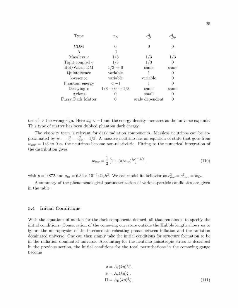
5.3 Examples
Cold dark matter provides a trivial example of a dark component. Here stress fluctuations are
negligible compared with the rest energy density and so wCDM = c2D = c2Dv = 0. Scalar field
dark energy provides another simple example. Here the competition between kinetic and potential
energy can drive wφ < 0. As we have already seen a slowly rolling scalar field has c2φ = 1 by virtue
of the absence of scalar field fluctuations in the rest gauge. In this case the fluctuations bear only
the kinetic contributions and so the relationship is exact.
The non-adiabatic sound speed c2D is also useful in characterizing k-essence, a scalar field with
a non-canonical kinetic term. Since in the rest gauge the potential fluctuation vanishes, the sound
speed directly reflects the modification to the kinetic term. A special case occurs when the kinetic
25
Type wD c2D c2Dv
CDM 0 0 0Λ -1 – –
Massless ν 1/3 1/3 1/3Tight coupled γ 1/3 1/3 0Hot/Warm DM 1/3 → 0 same sameQuintessence variable 1 0
k-essence variable variable 0Phantom energy < −1 1 0
Decaying ν 1/3 → 0 → 1/3 same sameAxions 0 small 0
Fuzzy Dark Matter 0 scale dependent 0
term has the wrong sign. Here wφ < −1 and the energy density increases as the universe expands.
This type of matter has been dubbed phantom dark energy.
The viscosity term is relevant for dark radiation components. Massless neutrinos can be ap-
proximated by wν = c2ν = c2νv = 1/3. A massive neutrino has an equation of state that goes from
wmν = 1/3 to 0 as the neutrinos become non-relativistic. Fitting to the numerical integration of
the distribution gives
wmν =1
3
[
1 + (a/anr)2p
]−1/p, (110)
with p = 0.872 and anr = 6.32 × 10⁻⁶/Ωνh2. We can model its behavior as c2mν = c2mνv = wD.
A summary of the phenomenological parameterization of various particle candidates are given
in the table.
5.4 Initial Conditions
With the equations of motion for the dark components defined, all that remains is to specify the
initial conditions. Conservation of the comoving curvature outside the Hubble length allows us to
ignore the microphysics of the intermediate reheating phase between inflation and the radiation
dominated universe. One can then simply take the initial conditions for structure formation to be
in the radiation dominated universe. Accounting for the neutrino anisotropic stress as described
in the previous section, the initial conditions for the total perturbations in the comoving gauge
become
δ = Aδ(kη)2ζ ,
v = Av(kη)ζ ,
Π = AΠ(kη)2ζ , (111)

26 Perturbation Theory
where δ = δρ/ρ, and η is now understood as the conformal time elapsed after the inflationary
epoch. The constants are
Aδ =4
9
1 + 2fν/15
1 + 4fν/15(1 − 3K/k2) ,
Av = −1
3
1
1 + 4fν/15,
AΠ = − 4
15
1
1 + 4fν/15, (112)
and
fν =ρν
ργ + ρν. (113)
The dark component initial conditions can then be determined by detailed balance
δJ = AδJ (kη)2ζ
vJ − v = A∆vJ (kη)3ζ ,
ΠJ = AΠJ(kη)2ζ (114)
with
AΠJ =c2JvwJ
AΠ ,
A∆vJ =
215 [2 − 3(wJ − c2J)](fν − 4
1+wJc2Jv) − [2(c2J − 1
3) + (wJ − c2J)](1 + 215fν)
(4 − 3c2J )[2 − 3(wJ − c2J)] + 9(c2J − c2Ja)c2J
(1 − 3K
k2)Av ,
AδJ =3
4(1 + wJ)
Aδ − 12(c2J − c2Ja)A∆vJ
1 − 3(wJ − c2J)/2. (115)
These initial conditions apply to all particle species J , including the photons and neutrinos, save
that for the baryons rapid Thomson scattering with the photons sets vb = vγ . In fact for most
numerical purposes one can simply set vJ − v = 0 in the initial conditions and let the velocity
differences arise dynamically in the integration. The initial conditions in an arbitrary gauge can be
established from these relations and the gauge transformation properties of the perturbations.
6 Cosmic Microwave Background
6.1 Boltzmann Equation
The gauge covariant formalism is useful for CMB studies as well. The interpretation of CMB
anisotropy formation is simplest in the Newtonian gauge where the manifestations of gravitational
redshift and infall correspond to Newtonian intuition. The numerical solution of the perturbation
equations is best handled under the comoving or synchronous gauge where the fundamental pertur-
bation variables are stable. The link to inflationary initial conditions is best seen in the comoving
gauge. The gauge covariant approach allows one to calculate in one gauge and interpret in or relate
to another.
Most of the physics of CMB perturbation evolution is contained in the general discussion of §2.
However the cosmic microwave background differs from the dark components in that it undergoes

27
interactions with the baryons that can exchange energy and momentum. Thus the conservation
law for its stress energy tensor must be supplemented with an interaction term. CMB observable
properties are also not the energy density and velocity perturbations but the higher order angular
distribution of its temperature and polarization.
Generally the CMB is described by the phase space distribution function photons in each of the
two polarization states fa(x,q, η), where x is the comoving position and q is the photon momentum.
The evolution of the distribution function under gravity and collisions is governed by the Boltzmann
equationd
dηfa,b = C[fa, fb] , (116)
where C denotes the collision term.
In absence of collisions, the Boltzmann equation becomes the Liouville equation. Rewriting the
variables in terms of the photon propagation direction n,
d
dηfa(x, n, q, η) = fa + ni∇ifa + q
∂
∂qfa = 0 . (117)
The last term represents the gravitational redshifting (or Sachs-Wolfe effect) of the photons under
the metric and is given by the geodesic equation as
q
q= − a
a− 1
2ninjHT ij − HL + niBi − ni∇iA . (118)
We have in fact already derived these gravitational effects in the general covariant perturbation
formalism. To establish this fact note that the stress energy tensor of the photons is the integral
of the photon distribution function over momentum states
T µν =
∫
d3q
(2π)3qµqν
E(fa + fb) . (119)
The Liouville equation then expresses the conservation of the stress-energy tensor. Given that the
CMB distribution is observed to be close to blackbody, it is suffices to calculate the evolution of
these integrated quantities. In particular let us define the temperature perturbation
Θ(x, n, η) =1
4δγ =
1
4ργ
∫
q3dq
2π2(fa + fb) − 1 (120)
and likewise for the linear polarization states Q and U as the temperature differences between
the polarization states. The redshift terms then become the metric terms in the continuity and
Navier-Stokes equations.
6.2 Eigenmodes
As in the case of the purely spatial perturbations, we decompose the temperature and polarization
in normal modes of the spatial and angular distributions. For the k-th spatial eigenmode
Θ(x, n, η) =∑
ℓm
Θ(m)ℓ Gmℓ (k,x, n) ,
[Q± iU ](x, n, η) =∑
ℓm
[E(m)ℓ ± iB
(m)ℓ ]±2G
mℓ (k,x, n) . (121)

28 Perturbation Theory
They are generated by recursion (0G = G)
ni( sGmℓ )|i =
q
2ℓ+ 1
[
sκmℓ ( sG
mℓ−1) − sκ
mℓ+1( sG
mℓ+1)
]
− iqms
ℓ(ℓ+ 1) sGmℓ , (122)
where
q2 = k2 + (|m| + 1)K ,
sκmℓ =
√
[
(ℓ2 −m2)(ℓ2 − s2)
ℓ2
] [
1 − ℓ2
q2K
]
. (123)
The lowest order modes begin the recursion and are related to the spatial harmonics as
0Gmj = ni1 . . . ni|m|Q
(m)i1...i|m|
,
±2Gm2 ∝ (m1 ± im2)
i1(m1 ± im2)i2Q
(m)i1i2
, (124)
where m1, m2 span the plane perpendicular to n. The normalization is set so that
sGmℓ (0, 0, n) = (−i)ℓ
√
4π
2ℓ+ 1 sYmℓ (n) . (125)
Here the spin spherical harmonics sYmℓ are the eigenfunctions of the 2D Laplace operator on a
rank s tensor. They are given explicitly by rotation matrices as
sYmℓ (θ, φ) =
√
2ℓ+ 1
4πDℓ
−ms(φ, θ, 0) . (126)
The meaning of these modes becomes clear in a spatially flat cosmology. Here the modes are
simply the direct product of plane waves and spin-spherical harmonics
Gmℓ (k,x, n) ≡ (−i)ℓ√
4π
2ℓ+ 1Y mℓ (n) exp(ik · x) ,
±2Gmℓ (k,x, n) ≡ (−i)ℓ
√
4π
2ℓ+ 1±2Y
mℓ (n) exp(ik · x) . (127)
The main content of the Liouville equation is purely geometrical and describes the projection of
inhomogeneities into anisotropies. Photon propagation takes gradients in the spatial distribution
and converts them to anisotropy as
n · ∇eik·x = in · keik·x = i
√
4π
3kY 0
1 (n)eik·x . (128)
This dipole term adds to angular dependence through the addition of angular momentum
√
4π
3Y 0
1 Ymℓ =
κmℓ√
(2ℓ+ 1)(2ℓ − 1)Y mℓ−1 +
κmℓ+1√
(2ℓ+ 1)(2ℓ + 3)Y mℓ+1 , (129)
where κmℓ = sκmℓ =
√ℓ2 −m2 is related to the Clebsch-Gordon coefficients.

29
6.3 Collision Term
The dominant collision process for CMB photons is Thomson scattering off of free electrons which
has the differential cross sectiondσ
dΩ=
3
8π|E′ · E|2σT , (130)
where E′ and E denote the incoming and outgoing directions of the electric field or polarization
vector.
To evaluate the collision term we begin in the electron rest frame and in a coordinate system
fixed by the scattering plane, spanned by incoming and outgoing directional vectors −n′ · n = cos β,
where β is the scattering angle. Denoting Θ‖ as the in-plane polarization temperature fluctuation
and Θ⊥ as the perpendicular polarization state, we obtain the geometrical content of the transfer
equation
Θ‖ ∝ cos2 βΘ′‖, Θ⊥ ∝ Θ′
⊥ , (131)
where the proportionality reflects the scattering rate
τ = neσTa . (132)
To calculate the Stokes parameters in this basis, we also need to calculate the polarization states
with axes rotated by 45
E1 =1√2(E‖ + E⊥) , E2 =
1√2(E‖ − E⊥) , (133)
yielding the transfer
Θ1 ∝ |E1 · E1|2Θ′1 + |E1 · E2|2Θ′
2
∝ 1
4(cos β + 1)2Θ′
1 +1
4(cos β − 1)2Θ′
2
Θ2 ∝ |E2 · E2|2Θ′2 + |E2 · E1|2Θ′
1
∝ 1
4(cos β + 1)2Θ′
2 +1
4(cos β − 1)2Θ′
1 . (134)
Now the transfer properties of the Stokes parameters
Θ ≡ 1
2(Θ‖ + Θ⊥), Q ≡ 1
2(Θ‖ − Θ⊥), U ≡ 1
2(Θ1 − Θ2) (135)
arranged in a vector T ≡ (Θ, Q+ iU , Q− iU) becomes
T ∝ S(β)T′ , (136)
S(β) =3
4
cos2 β + 1 −12 sin2 β −1
2 sin2 β−1
2 sin2 β 12(cos β + 1)2 1
2(cos β − 1)2
−12 sin2 β 1
2(cos β − 1)2 12(cos β + 1)2
,
where the normalization factor is set by photon conservation in the scattering.

30 Perturbation Theory
Finally convert the the polarization quantities referenced to the scattering basis to a fixed basis
on the sky by noting that under a rotation T′ = R(ψ)T where
R(ψ) =
1 0 00 e−2iψ 00 0 e2iψ
, (137)
giving the scattering matrix
R(−γ)S(β)R(α) =
1
2
√
4π
5
Y 02 (β, α) + 2
√5Y 0
0 (β, α) −√
32Y
−22 (β, α) −
√
32Y
22 (β, α)
−√
6 2Y02 (β, α)e2iγ 3 2Y
−22 (β, α)e2iγ 3 2Y
22 (β, α)e2iγ
−√
6−2Y02 (β, α)e−2iγ 3 −2Y
−22 (β, α)e−2iγ 3 −2Y
22 (β, α)e−2iγ
, (138)
where α, γ are the angles required to rotate into and out of the scattering frame.
Finally, by employing the addition theorem for spin spherical harmonics
∑
m
s1Y m∗
ℓ (n′) s2Y m
ℓ (n) = (−1)s1−s2
√
2ℓ+ 1
4π s2Y −s1
ℓ (β, α)eis2γ (139)
the scattering in the electron rest frame into the Stokes states becomes
Cin[T] = τ
∫
dn′
4πR(−γ)S(β)R(α)T(n′)
= τ
∫
dn′
4π(Θ′, 0, 0) +
1
10τ
∫
dn′2
∑
m=−2
P(m)(n, n′)T(n′) , (140)
where the quadrupole coupling term is
P(m)(n, n′) =
Y m∗2 (n′)Y m
2 (n) −√
32 2Y
m∗2 (n′)Y m
2 (n) −√
32 −2Y
m∗2 (n′)Y m
2 (n)
−√
6Y m∗2 (n′) 2Y
m2 (n) 3 2Y
m∗2 (n′) 2Y
m2 (n) 3 −2Y
m∗2 (n′) 2Y
m2 (n)
−√
6Y m∗2 (n′)−2Y
m2 (n) 3 2Y
m∗2 (n′)−2Y
m2 (n) 3 −2Y
m∗2 (n′)−2Y
m2 (n)
. (141)
The full scattering matrix involves difference of scattering into and out of state
C[T] = Cin[T] − Cout[T] . (142)
In the electron rest frame
C[T] = τ
∫
dn′
4π(Θ′, 0, 0)− τT + CP [T] (143)
which describes isotropization in the rest frame. All moments have e−τ suppression except for isotropictemperature Θ0. Here CP is the P or ℓ = 2 term of Eqn. (140).
Transformation into the background frame simply induces a dipole term
C[T] = τ
(
n · vb +
∫
dn′
4πΘ′, 0, 0
)
− τT + CP [T] , (144)
yielding the final form of the collision term.

31
6.4 Temperature-Polarization Hierarchy
The Boltzmann equation in normal modes then becomes
Θ(m)ℓ = q
[
κmℓ
2ℓ+ 1Θ
(m)ℓ−1 −
κmℓ+1
2ℓ+ 3Θ
(m)ℓ+1
]
− τΘ(m)ℓ + S
(m)ℓ ,
E(m)ℓ = k
[
2κmℓ
2ℓ− 1E
(m)ℓ−1 − 2m
ℓ(ℓ+ 1)B
(m)ℓ − 2κ
mℓ+1
2ℓ+ 3
]
− τE(m)ℓ + E(m)
ℓ ,
B(m)ℓ = k
[
2κmℓ
2ℓ− 1B
(m)ℓ−1 +
2m
ℓ(ℓ+ 1)B
(m)ℓ − 2κ
mℓ+1
2ℓ+ 3
]
− τE(m)ℓ + B(m)
ℓ , (145)
where the gravitational and scattering sources are
S(m)ℓ =
τΘ(0)0 − H
(0)L τ v
(0)b + B(0) τP (0) − 2
3
√
1 − 3K/k2H(0)T
0 τ v(±1)b + B(±1) τP (±1) −
√3
3
√
1 − 2K/k2H(±1)T
0 0 τP (±2) − H(±2)T
,
E(m)ℓ = −τ
√6P (m)δℓ,2 ,
B(m)ℓ = 0 , (146)
with
P (m) ≡ 1
10(Θ
(m)2 −
√6E
(m)2 ) . (147)
The physical content of the coupling hierarchy is that an inhomogeneity in the temperature or polariza-tion distribution will eventually become a high multipole order anisotropy by “free streaming” or simpleprojection.
6.5 Integral Solution
Since the hierarchy equations simply represents geometric projection, their implicit solution can be writtenas the projection of the gravitational and scattering sources at a distance. This operation proceeds by writingthe normal modes themselves in spherical coordinates,
Gmℓs
=∑
ℓ
(−i)ℓ√
4π(2ℓ+ 1)α(m)ℓsℓ (k,D)Y m
ℓ (n) ,
±2Gmℓs
=∑
ℓ
(−i)ℓ√
4π(2ℓ+ 1)[ǫ(m)ℓsℓ ± β
(m)ℓsℓ ](k,D)±2Y
mℓ (n) , (148)
where D = η0 − η. Summing over the sources
Θ(m)ℓ (k, η0)
2ℓ+ 1=
∫ η0
0
dηe−τ∑
ℓs
S(m)ℓs
α(m)ℓsℓ (k,D) ,
E(m)ℓ (k, η0)
2ℓ+ 1=
∫ η0
0
dηe−τ∑
ℓs
E(m)ℓs
ǫ(m)ℓsℓ (k,D) ,
B(m)ℓ (k, η0)
2ℓ+ 1=
∫ η0
0
dηe−τ∑
ℓs
E(m)ℓs
β(m)ℓsℓ (k,D) . (149)
Note that the polarization has only an ℓs = 2 source.In a flat cosmology, the radial projection kernels are related to spherical Bessel functions
eik·x =∑
ℓ
(−i)ℓ√
4π(2ℓ+ 1)jℓ(kD)Y 0ℓ (n) (150)

32 Perturbation Theory
by the recoupling of the “spin” angular dependence of the source ℓs to the “orbital” angular dependence ofthe plane waves. For example
α(0)0ℓ (k,D) ≡ jℓ(kD) ,
α(0)1ℓ (k,D) ≡ j′ℓ(kD) ,
ǫ(0)2ℓ (k,D) =
√
3
8
(ℓ+ 2)!
(ℓ− 2)!
jℓ(kD)
(kD)2,
β(0)2ℓ (k,D) = 0 . (151)
In a curved geometry, the radial projection kernels are related to the ultraspherical Bessel functions by thesame coupling of angular momenta.
6.6 Power Spectra
The two point statistics of the temperature and polarization fields are described by their power spectra
CXX′
ℓ =2
π
∫
dk
k
∑
m
k3〈X(m)∗ℓ X
′(m)ℓ 〉
(2ℓ+ 1)2, (152)
where X,X ′ ∈ Θ, E,B.
7 Epilogue
How to conclude Lecture notes in which no conclusions have been drawn? I leave you instead with a thought:
What goes on being hateful about analysis is that it implies that the analyzed is a completedset. The reason why completion goes on being hateful is that it implies everything can be acompleted set.
–Chuang-tzu, 23
8 Acknowledgments
I thank the organizers and participants of the Trieste school, my collaborators over the years (especially D.Eisenstein, N. Sugiyama and M. White in this context), and the long-suffering students of AST448 at U.Chicago.

33
References
[1] J.M. Bardeen, “Gauge Invariant Cosmological Perturbations,” Phys. Rev. D, 22, 1882 (1980).
[2] H. Kodama, M. Sasaki, “Cosmological Perturbation Theory,” Prog. Theor. Phys. Suppl., 78, 1 (1984).
[3] W. Hu, D.J. Eisenstein, “The Structure of Structure Formation Theories,” Phys. Rev. D, 52, 083509(1999).
[4] V.F. Mukhanov, H.A. Feldman, R.H. Brandenberger, “Theory of Cosmological Perturbations,” Phys.Rept., 215, 203 (1992).
[5] W. Hu, “Structure Formation with Generalized Dark Matter,” Astrophys. J, 506, 485 (1998).
[6] W. Hu, U. Seljak, M. White, M. Zaldarriaga, “A Complete Treatment of CMB Anisotropies in a FRWUniverse,” Phys. Rev. D, 57, 3290 (1998).
[7] P.J.E. Peebles, J.T. Yu, “Primeval Adiabatic Perturbation in an Expanding Universe,” Astrophys. J,162, 815 (1970).