1

Coverage control for mobile sensing networksJorge Cortes,Member IEEE, Sonia Martınez,Member IEEE, Timur Karatas, Francesco Bullo,Member IEEE

Abstract—This paper presents control and coordination algo-rithms for groups of vehicles. The focus is on autonomous vehiclenetworks performing distributed sensing tasks where each vehicleplays the role of a mobile tunable sensor. The paper proposesgradient descent algorithms for a class of utility functions whichencode optimal coverage and sensing policies. The resultingclosed-loop behavior is adaptive, distributed, asynchronous, andverifiably correct.

Index Terms—Coverage control, distributed and asynchronousalgorithms, sensor networks, centroidal Voronoi partitions

I. I NTRODUCTION

Mobile sensing networks

The deployment of large groups of autonomous vehicles israpidly becoming possible because of technological advancesin networking and in miniaturization of electro-mechanicalsystems. In the near future, large numbers of robots willcoordinate their actions through ad-hoc communication net-works and will perform challenging tasks including search andrecovery operations, manipulation in hazardous environments,exploration, surveillance, and environmental monitoringforpollution detection and estimation. The potential advantages ofemploying teams of agents are numerous. For instance, certaintasks are difficult, if not impossible, when performed by asingle vehicle agent. Further, a group of vehicles inherentlyprovides robustness to failures of single agents or communi-cation links.

Working prototypes of active sensing networks have alreadybeen developed; see [1], [2], [3], [4]. In [3], launchableminiature mobile robots communicate through a wireless net-work. The vehicles are equipped with sensors for vibrations,acoustic, magnetic, and IR signals as well as an active videomodule (i.e., the camera or micro-radar is controlled via apan-tilt unit). A second system is suggested in [4] underthe name of Autonomous Oceanographic Sampling Network.In this case, underwater vehicles are envisioned measuringtemperature, currents, and other distributed oceanographicsignals. The vehicles communicate via an acoustic local area

Submitted on November 4, 2002, revised on June 16, 2003. Appeared in theIEEE Transactions on Robotics and Automation, vol 20, issue 2, year 2004,pages 243–255. This version contains minor corrections and was generatedon April 24, 2008. Previous short versions of this paper appeared in theIEEE Conference on Robotics and Automation, Arlington, VA, May 2002,and Mediterranean Conference on Control and Automation, Lisbon, Portugal,July 2002.

Jorge Cortes, Timur Karatas and Francesco Bullo are with the Coor-dinated Science Laboratory, University of Illinois at Urbana-Champaign,1308 W. Main St., Urbana, IL 61801, United States, Tels: +1-217-244-8734, +1-217-244-9414 and +1-217-333-0656, Fax: +1-217-244-1653, Email:jcortes,tkaratas,bullo@uiuc.edu

Sonia Martınez is with the Escola Universitaria Politecnica de Vilanova ila Geltru, Universidad Politecnica de Cataluna, Av. V. Balaguer s/n, Vilanovai la Geltru, 08800, Spain, Tel: +34-938967743, Fax: +34-938967700, Email:soniam@mat.upc.es

network and coordinate their motion in response to localsensing information and to evolving global data. This mobilesensing network is meant to provide the ability to samplethe environment adaptively in space and time. By identifyingevolving temperature and current gradients with higher accu-racy and resolution than current static sensors, this technologycould lead to the development and validation of improvedoceanographic models.

Optimal sensor allocation and coverage problems

A fundamental prototype problem in this paper is that ofcharacterizing and optimizing notions of quality-of-serviceprovided by an adaptive sensor network in a dynamic en-vironment. To this goal, we introduce a notion ofsensorcoveragethat formalizes an optimal sensor placement problem.This spatial resource allocation problem is the subject of adiscipline called locational optimization [5], [6], [7], [8], [9].

Locational optimization problems pervade a broad spectrumof scientific disciplines. Biologists rely on locational optimiza-tion tools to study how animals share territory and to char-acterize the behavior of animal groups obeying the followinginteraction rule: each animal establishes a region of dominanceand moves toward its center. Locational optimization problemsare spatial resource allocation problems (e.g., where to placemailboxes in a city or cache servers on the internet) and playacentral role in quantization and information theory (e.g.,howto design a minimum-distortion fixed-rate vector quantizer).Other technologies affected by locational optimization includemesh and grid optimization methods, clustering analysis, datacompression, and statistical pattern recognition.

Because locational optimization problems are so widelystudied, it is not surprising that methods are indeed availableto tackle coverage problems; see [5], [8], [10], [9]. How-ever, most currently-available algorithms are not applicableto mobile sensing networks because they inherently assumea centralized computation for a limited size problem in aknown static environment. This is not the case in multi-vehiclenetworks which, instead, rely on a distributed communicationand computation architecture. Although an ad-hoc wirelessnetwork provides the ability to share some information, noglobal omniscient leader might be present to coordinate thegroup. The inherent spatially-distributed nature and limitedcommunication capabilities of a mobile network invalidateclassic approaches to algorithm design.

Distributed asynchronous algorithms for coverage control

In this paper we design coordination algorithms imple-mentable by a multi-vehicle network with limited sensing andcommunication capabilities. Our approach is related to theclassic Lloyd algorithm from quantization theory; see [11]

2

for a reprint of the original report and [12] for a historicaloverview. We present Lloyd descent algorithms that take intocareful consideration all constraints on the mobile sensingnetwork. In particular, we design coverage algorithms thatareadaptive, distributed, asynchronous, and verifiably asymptoti-cally correct:

Adaptive: Our coverage algorithms provide the network withthe ability to address changing environments, sensingtask, and network topology (due to agents departures,arrivals, or failures).

Distributed: Our coverage algorithms are distributed in thesense that the behavior of each vehicle depends only onthe location of its neighbors. Also, our algorithms donot require a fixed-topology communication graph, i.e.,the neighborhood relationships do change as the networkevolves. The advantages of distributed algorithms arescalability and robustness.

Asynchronous: Our coverage algorithms are amenable toasynchronous implementation. This means that the algo-rithms can be implemented in a network composed ofagents evolving at different speeds, with different compu-tation and communication capabilities. Furthermore, ouralgorithms do not require a global synchronization andconvergence properties are preserved even if informationabout neighboring vehicles propagates with some delay.An advantage of asynchronism is a minimized commu-nication overhead.

Verifiable Asymptotically Correct: Our algorithms guaran-tee monotonic descent of the cost function encodingthe sensing task. Asymptotically, the evolution of themobile sensing network is guaranteed to converge to so-called centroidal Voronoi configurations (i.e., configura-tions where the location of each generator coincides withthe centroid of the corresponding Voronoi cell) that arecritical points of the optimal sensor coverage problem.

Let us describe in some detail what are the contributions ofthis paper. Section II reviews certain locational optimizationproblems and their solutions as centroidal Voronoi partitions.Section III provides a continuous-time version of the classicLloyd algorithm from vector quantization and applies it to thesetting of multi-vehicle networks. In discrete-time, we pro-pose a family of Lloyd algorithms. We carefully characterizeconvergence properties for both continuous and discrete-timeversions (Appendix A collects some relevant facts on descentflows). We discuss a worst-case optimization problem, weinvestigate a simple uniform planar setting, and we presentsimulation results.

Section IV presents two asynchronous distributed imple-mentations of Lloyd algorithm for ad-hoc networks withcommunication and sensing capabilities. Our treatment care-fully accounts for the constraints imposed by the distributednature of the vehicle network. We present two asynchronousimplementations, one based on classic results on distributedgradient flows, the other based on the structure of the coverageproblem. (Appendix B briefly reviews some known results onasynchronous gradient algorithms.)

Section V-A considers vehicle models with more realisticdynamics. We present two formal results on passive vehicledynamics and on vehicles equipped with individual local con-trollers. We present numerical simulations of passive vehiclemodels and of unicycle mobile vehicles. Next, Section V-B de-scribes density functions that lead the multi-vehicle network topredetermined geometric patterns. We present our conclusionsand directions for future research in Section VI.

Review of distributed algorithms for cooperative control

Recent years have witnessed a large research effort focusedon motion planning and coordination problems for multi-vehicle systems. Issues include geometric patterns [13], [14],[15], [16], formation control [17], [18], gradient climbing [19],and conflict avoidance [20]. It is only recently, however, thattruly distributed coordination laws for dynamic networks arebeing proposed; e.g., see [21], [22], [23].

Heuristic approaches to the design of interaction rules andemerging behaviors have been throughly investigated withinthe literature on behavior-based robotics; see [24], [25],[17],[26], [27], [28]. An example of coverage control is discussedin [29]. Along this line of research, algorithms have beendesigned for sophisticated cooperative tasks. However, noformal results are currently available on how to design reactivecontrol laws, ensure their correctness, and guarantee theiroptimality with respect to an aggregate objective.

The study of distributed algorithms is concerned with pro-viding mathematical models, devising precise specificationsfor their behavior, and formally proving their correctnessandcomplexity. Via an automata-theoretic approach, the refer-ences [30], [31] treat distributed consensus, resource alloca-tion, communication, and data consistency problems. Froma numerical optimization viewpoint, the works in [32], [33]discuss distributed asynchronous algorithms as networkingalgorithms, rate and flow control, and gradient descent flows.Typically, both these sets of references consider networkswithfixed topology, and do not address algorithms over ad-hoc dy-namically changing networks. Another common assumption isthat any time an agent communicates its location, it broadcastsit to every other agent in the network. In our setting, this wouldrequire a non-distributed communication set-up.

Finally, we note that the terminology “coverage” is alsoused in [34], [35] and references therein to refer to a differentproblem called thecoverage path planning problem, where asingle robot equipped with a limited footprint sensor needstovisit all points in its environment.

II. FROM LOCATION OPTIMIZATION TO CENTROIDAL

VORONOI PARTITIONS

A. Locational optimization

In this section we describe a collection of known factsabout a meaningful optimization problem. References includethe theory and applications of centroidal Voronoi partitions,see [10], and the discipline of facility location, see [6]. Alongthe paper, we interchangeably refer to the elements of thenetwork as sensors, agents, vehicles, or robots. We letR+ be

3

the set of nonnegative real numbers,N be the set of positivenatural numbers andN0 = N ∪ 0.

Let Q be a convex polytope inRN including its interior, andlet ‖ ·‖ denote the Euclidean distance function. We call a mapφ : Q → R+ a distribution density functionif it representsa measure of information or probability that some event takeplace overQ. In equivalent words, we can considerQ to bethe bounded support of the functionφ. Let P = (p1, . . . , pn)be the location of n sensors, each moving in the spaceQ.Because of noise and loss of resolution, thesensing perfor-manceat point q taken from ith sensor at the positionpi

degrades with the distance‖q − pi‖ betweenq and pi; wedescribe this degradation with a non-decreasing differentiablefunction f : R+ → R+. Accordingly,f (‖q − pi‖) provides aquantitative assessment of how poor the sensing performanceis.

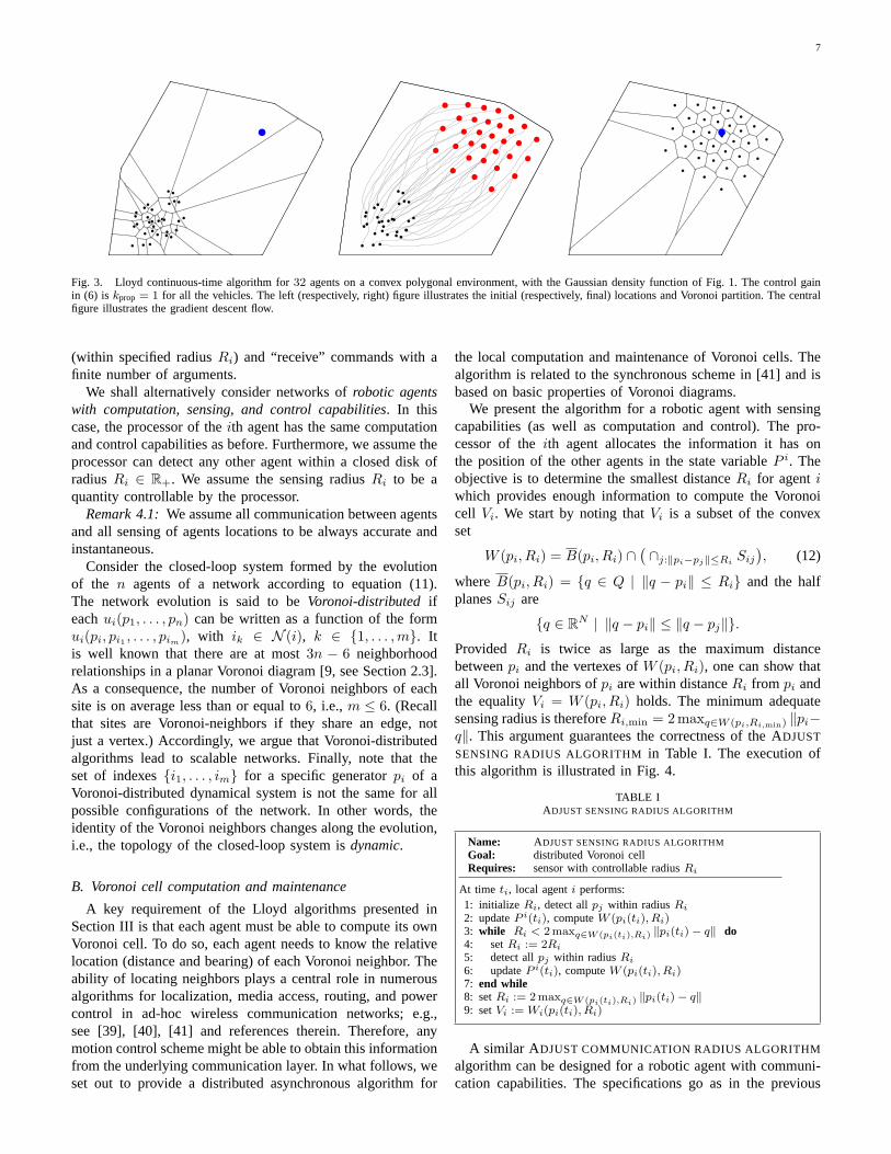
Fig. 1. Contour plot on a polygonal environment of the Gaussian densityfunction φ = exp(−x2 − y2).

Remark 2.1:As an example, considern mobile robotsequipped with microphones attempting to detect, identify,andlocalize a sound-source.How should we plan to robots’ motionin order to maximize the detection probability?Assuming thesource emits a known signal, the optimal detection algorithmis a matched filter (i.e., convolve the known waveform withthe received signal and threshold). The source is detecteddepending on the signal-to-noise-ratio, which is inverselyproportional to the distance between the microphone andthe source. Various electromagnetic and sound sensors havesignal-to-noise ratios inversely proportional to distance.

Within the context of this paper, apartition of Q is acollection of n polytopesW = W1, . . . ,Wn with disjointinteriors whose union isQ. We say that two partitionsW andW ′ are equal ifWi andW ′

i only differ by a set ofφ-measurezero, for alli ∈ 1, . . . , n.

We consider the task of minimizing the locational optimiza-tion function

H(P,W) =n∑

i=1

∫

Wi

f(‖q − pi‖)φ(q)dq, (1)

where we assume that theith sensor is responsible for mea-surements over its “dominance region”Wi. Note that thefunction H is to be minimized with respect to both (1) thesensors locationP , and (2) the assignment of the dominanceregionsW. The optimization is therefore to be performed withrespect to the position of the sensors and the partition of thespace. This problem is referred to as a facility location problemand in particular as a continuousp-median problem in [6].

Remark 2.2:Note that if we interchange the positionsof any two agents, along with their associatedregions of dominance, the value of the locationaloptimization function H is not affected. Equivalently,if Σn denotes the discrete group of permutationsof n elements, then H(p1, . . . , pn,W1, . . . ,Wn) =H(pσ(1), . . . , pσ(n),Wσ(1), . . . ,Wσ(n)) for all σ ∈ Σn.To eliminate this discrete redundancy, one could take naturalaction ofΣn on Qn, and considerQn/Σn as the configurationspace for the positionP of the n vehicles.

B. Voronoi partitions

One can easily see that, at fixed sensors location, the optimalpartition of Q is the Voronoi partitionV(P ) = V1, . . . , Vngenerated by the points(p1, . . . , pn):

Vi = q ∈ Q | ‖q − pi‖ ≤ ‖q − pj‖ , ∀j 6= i.

We refer to [9] for a comprehensive treatment on Voronoidiagrams, and briefly present some relevant concepts. The setof regionsV1, . . . , Vn is called the Voronoi diagram for thegeneratorsp1, . . . , pn. When the two Voronoi regionsVi

and Vj are adjacent (i.e., they share an edge),pi is called a(Voronoi) neighborof pj (and vice-versa). The set of indexesof the Voronoi neighbors ofpi is denoted byN (i). Clearly,j ∈ N (i) if and only if i ∈ N (j). We also define the(i, j)-face as∆ij = Vi ∩ Vj . Voronoi diagrams can be defined withrespect to various distance functions, e.g., the1-, 2-, s-, and∞-norm overQ = R

m, see [36]. Some useful facts about theEuclidean setting are the following: ifQ is a convex polytopein a N -dimensional Euclidean space, the boundary of eachVi

is the union of(N − 1)-dimensional convex polytopes.In what follows, we shall write

HV(P ) = H(P,V(P )).

Note that using the definition of the Voronoi partition, wehavemini∈1,...,n f(‖q − pi‖) = f(‖q − pj‖) for all q ∈ Vj .Therefore,

HV(P ) =

∫

Q

mini∈1,...,n

f(‖q − pi‖)φ(q)dq , (2)

= E(Q,φ)

[

mini∈1,...,n

f(‖q − pi‖)

]

,

that is, the locational optimization function can be interpretedas an expected value composed with a min operation. This isthe usual way in which the problem is presented in the facilitylocation and operations research literature [6]. Remarkably,one can show [10] that

∂HV

∂pi

(P ) =∂H

∂pi

(P,V(P )) =

∫

Vi

∂

∂pi

f (‖q − pi‖) φ(q)dq,

(3)

i.e., the partial derivative ofHV with respect to theith sensoronly depends on its own position and the position of itsVoronoi neighbors. Therefore the computation of the derivativeof HV with respect to the sensors’ location is decentralizedin the sense of Voronoi. Moreover, one can deduce somesmoothness properties ofHV : since the Voronoi partitionV depends at least continuously onP = (p1, . . . , pn), thefunctionHV is at least continuously differentiable.

4

C. Centroidal Voronoi partitions

Let us recall some basic quantities associated to a regionV ⊂ R

N and a mass density functionρ. The (generalized)mass, centroid (or center of mass), and polar moment of inertiaare defined as

MV =

∫

V

ρ(q) dq, CV =1

MV

∫

V

q ρ(q) dq,

JV,p =

∫

V

‖q − p‖2 ρ(q) dq.

Additionally, by the parallel axis theorem, one can write,

JV,p = JV,CV+ MV ‖p − CV ‖2 (4)

whereJV,CV∈ R+ is defined as the polar moment of inertia

of the regionV about its centroidCV .Let us consider again the locational optimization prob-

lem (1), and suppose now we are strictly interested in thesetting

H(P,W) =

n∑

i=1

∫

Wi

‖q − pi‖2φ(q)dq, (5)

that is, we assumef(‖q− pi‖) = ‖q− pi‖2. The parallel axis

theorem leads to simplifications for both the functionHV andits partial derivative:

HV(P ) =

n∑

i=1

JVi,CVi+

n∑

i=1

MVi‖pi − CVi

‖2

∂HV

∂pi

(P ) = 2MVi(pi − CVi

).

Here the mass density function isρ = φ. It is convenient todefine

HV,1 =

n∑

i=1

JVi,CVi, HV,2 =

n∑

i=1

MVi‖pi − CVi

‖2 .

Therefore, the (not necessarily unique) local minimum pointsfor the location optimization functionHV arecentroidsof theirVoronoi cells, i.e., each locationpi satisfies two propertiessimultaneously: it is the generator for the Voronoi cellVi andit is its centroid

CVi= argminpi

HV(P ).

Accordingly, the critical partitions and points forH are calledcentroidal Voronoi partitions. We will refer to a sensors’configuration as acentroidal Voronoi configurationif it givesrise to a centroidal Voronoi partition. Of course, centroidalVoronoi configurations depend on the specific distribution den-sity functionφ, and an arbitrary pair(Q,φ) admits in generalmultiple centroidal Voronoi configurations. This discussionprovides a proof alternative to the one given in [10] for thenecessity of centroidal Voronoi partitions as solutions tothecontinuousp-median location problem.

III. C ONTINUOUS AND DISCRETE-TIME LLOYD DESCENT

FOR COVERAGE CONTROL

In this section, we describe algorithms to compute thelocation of sensors that minimize the costH, both in con-tinuous and in discrete-time. In Section III-A, we propose a

continuous-time version of the classic Lloyd algorithm. Here,both the positions and partitions evolve in continuous time,whereas Lloyd algorithm for vector quantization is designedin discrete time. In Section III-B, we develop a family ofvariations of Lloyd algorithm in discrete time. In both settings,we prove that the proposed algorithms aregradient descentflows.

A. A continuous-time Lloyd algorithm

Assume the sensors location obeys a first order dynamicalbehavior described by

pi = ui.

ConsiderHV a cost function to be minimized and imposethat the locationpi follows a gradient descent. In equivalentcontrol theoretical terms, considerHV a Lyapunov functionand stabilize the multi-vehicle system to one of its localminima via dissipative control. Formally, we set

ui = −kprop(pi − CVi), (6)

wherekprop is a positive gain, and where we assume that thepartitionV(P ) = V1, . . . , Vn is continuously updated.

Proposition 3.1 (Continuous-time Lloyd descent):For theclosed-loop system induced by equation (6), the sensors lo-cation converges asymptotically to the set of critical pointsof HV , i.e., the set of centroidal Voronoi configurations onQ.Assuming this set is finite, the sensors location converges toa centroidal Voronoi configuration.

Proof: Under the control law (6), we have

d

dtHV(P (t)) =

n∑

i=1

∂HV

∂pi

pi

= −2kprop

n∑

i=1

MVi‖pi − CVi

‖2 = −2kpropHV,2(P (t)).

By LaSalle’s principle, the sensors location converges to thelargest invariant set contained inH−1

V,2(0), which is preciselythe set of centroidal Voronoi configurations. Since this setisclearly invariant for (6), we get the stated result. IfH−1

V,2(0)consists of a finite collection of points, thenP (t) convergesto one of them, see Corollary A.2.

Remark 3.2:If H−1V,2(0) is finite, andP (t) → C, then a

sufficient condition that guarantees exponential convergence isthat the Hessian ofHV be positive definite atC. Establishingthis property is a known open problem, see [10]. Note that thisgradient descent is not guaranteed to find the global minimum.For example, in the vector quantization and signal processingliterature [12], it is known that for bimodal distribution densityfunctions, the solution to the gradient flow reaches localminima where the number of generators allocated to the tworegion of maxima are not optimally partitioned.

B. A family of discrete-time Lloyd algorithms

Let us consider the following variations of Lloyd algorithm.Let T be a continuous mappingT : Qn → Qn verifying thefollowing two properties:

5

(a) for all i ∈ 1, . . . , n, ‖Ti(P )−CVi(P )‖ ≤ ‖pi−CVi(P )‖, whereTi denotes theith component ofT ,(b) if P is not centroidal, then there exists aj suchthat ‖Tj(P ) − CVj(P )‖ < ‖pj − CVj(P )‖.

Property (a) guarantees that, if moved according toT , theagents of the network do not increase their distance to itscorresponding centroid. Property (b) ensures that at leastonerobot moves at each iteration and strictly approaches the cen-troid of its Voronoi region. Because of this property, the fixedpoints ofT are the set of centroidal Voronoi configurations.

Proposition 3.3 (Discrete-time Lloyd descent):Let T :Qn → Qn be a continuous mapping satisfying properties (a)and (b). LetP0 ∈ Qn denote the initial sensors’ location.Then, the sequenceTm(P0) | m ∈ N converges to the setof centroidal Voronoi configurations. If this set is finite, thenthe sequenceTm(P0) | m ∈ N converges to a centroidalVoronoi configuration.

Proof: Consider HV : Qn → R+ as an objectivefunction for the algorithmT . Using the parallel axis theorem,H(P,W) =

∑ni=1 JWi,CWi

+∑n

i=1 MWi‖pi − CWi

‖2, andtherefore

H(P ′,W) ≤ H(P,W) , (7)

as long as‖p′i − CWi‖ ≤ ‖pi − CWi

‖ for all i ∈ 1, . . . , n,with strict inequality if for anyi, ‖p′i −CWi

‖ < ‖pi −CWi‖.

In particular,H(CW ,W) ≤ H(P,W), with strict inequalityif P 6= CW , where CW denotes the set of centroids ofthe partitionW. Moreover, since the Voronoi partition is theoptimal one for fixedP , we also have

H(P,V(P )) ≤ H(P,W) , (8)

with strict inequality ifW 6= V(P ).Now, because of property (a) ofT , inequality (7) yields

H(T (P ),V(P )) ≤ H(P,V(P )) = HV(P ) ,

and the inequality is strict ifP is not centroidal by property(b) of T . In addition,

HV(T (P )) = H(T (P ),V(T (P ))) ≤ H(T (P ),V(P )) ,

because of (8). Hence,HV(T (P )) ≤ HV(P ), and the inequal-ity is strict if P is not centroidal. We then conclude thatHV isa descent function for the algorithmT . The result now followsfrom the global convergence Theorem A.3 and Proposition A.4in Appendix A.

Remark 3.4:Lloyd algorithm in quantization theory [11],[12] is usually presented as follows: given the location ofnagents,p1, . . . , pn, (i) construct the Voronoi partition corre-sponding toP = (p1, . . . , pn); (ii) compute the mass centroidsof the Voronoi regions found in step (i). Set the new locationof the agents to these centroids; and return to step (i). Lloydalgorithm can also be seen as a fixed point iteration. Considerthe mappingsLLi : Qn → Q for i ∈ 1, . . . , n

LLi(p1, . . . , pn) =

(

∫

Vi(P )

φ(q)dq

)−1∫

Vi(P )

qφ(q)dq .

Let LL : Qn → Qn be defined byLL = (LL1, . . . , LLn).Clearly, LL is continuous (indeed,C1), and corresponds to

Lloyd algorithm. Now,‖LLi(P ) − CVi‖ = 0 ≤ ‖pi − CVi

‖,for all i ∈ 1, . . . , n. Moreover, ifP is not centroidal, thenthe inequality is strict for allpi 6= CVi

. Therefore,LL verifiesproperties (a) and (b).

C. Remarks

(i) Note that different sensor performance functionsf inequation (1) correspond to different optimization prob-lems. Provided one uses the Euclidean distance in thedefinition ofH (cf. equation (1)), the standard Voronoipartition computed with respect to the Euclidean metricremains the optimal partition. For arbitraryf , it is notpossible anymore to decomposeHV into the sum ofterms similar toHV,1 and HV,2. Nevertheless, it isstill possible to implement the gradient flow via theexpression for the partial derivative (3).Proposition 3.5: Assume the sensors location obeys afirst order dynamical behavior,pi = ui. Then, for theclosed-loop system induced by the gradient law (3),ui = −∂HV/∂pi, the sensors locationP = (p1, . . . , pn)converges asymptotically to the set of critical points ofHV . Assuming this set is finite, the sensors locationconverges to a critical point.

(ii) More generally, various distance notions can be usedto define locational optimization functions. Differentperformance function gives rise to corresponding notionsof “center of a region” (any notion of geometric center,mean, or average is an interesting candidate). These canthen be adopted in designing coverage algorithms. Werefer to [36] for a discussion on Voronoi partitions basedon non-Euclidean distance functions and to [5], [8] for adiscussion on the corresponding locational optimizationproblems.

(iii) Next, let us discuss an interesting variation of the origi-nal problem. In [6], minimizing the expected minimumdistance functionHV in equation (2) is referred toas thecontinuousp-median problem. It is instructiveto consider the worst-case minimum distance function,corresponding to the scenario where no information isavailable on the distribution density function. In otherwords, the network seeks to minimize the largest possi-ble distance from any point inQ to any of the sensorlocations, i.e., to minimize the function

maxq∈Q

[

mini∈1,...,n

‖q − pi‖

]

= maxi∈1,...,n

[

maxq∈Vi

‖q − pi‖

]

.

This optimization is referred to as thep-center problemin [6], [7]. One can design a strategy for thep-centerproblem analog to the Lloyd algorithm for thep-medianproblem: each vehicle moves, in continuous or discrete-time, toward the center of the minimum-radius sphereenclosing the polytope. We refer to [37] for a conver-gence analysis of the continuous-time algorithms.

In what follows, we shall restrict our attention to thep-median problem and to centroidal Voronoi partitions.

6

D. Computations over polygons with uniform density

In this section, we investigate closed-form expression forthecontrol laws introduced above. Assume the Voronoi regionVi

is a convex polygon (i.e., a polytope inR2) with Ni vertexeslabeled(x0, y0), . . . , (xNi−1, yNi−1) such as in Fig. 2. It isconvenient to define(xNi

, yNi) = (x0, y0). Furthermore, we

assume that the density function isφ(q) = 1. By evaluating the

(x2, y2)

(x3, y3)

(x5, y5)(x0, y0) = (x6, y6)

(x1, y1)

(Cx, Cy)

(x4, y4)

Fig. 2. Notation conventions for a convex polygon.

corresponding integrals, one can obtain the following closed-form expressions

MVi=

1

2

Ni−1∑

k=0

(xkyk+1 − xk+1yk)

CVi,x =1

6MVi

Ni−1∑

k=0

(xk + xk+1)(xkyk+1 − xk+1yk) (9)

CVi,y =1

6MVi

Ni−1∑

k=0

(yk + yk+1)(xkyk+1 − xk+1yk) .

To present a simple formula for the polar moment of inertia,let xk = xk−CVi,x andyk = yk−CVi,y, for k ∈ 0, . . . , Ni−1. Then, the polar moment of inertia of a polygon about itscentroid,JVi,C becomes

JVi,CVi=

1

12

Ni−1∑

k=0

(xkyk+1 − xk+1yk) ·

(x2k + xkxk+1 + x2

k+1 + y2k + ykyk+1 + y2

k+1) .

The proof of these formulas is based on decomposing thepolygon into the union of disjoint triangles. We refer to [38]for analog expressions overR

N .Note also that the Voronoi polygon’s vertexes can be ex-

pressed as a function of the neighboring vehicles. The vertexesof the ith Voronoi polygon that lie in the interior ofQ arethe circumcenters of the triangles formed bypi and any twoneighbors adjacent topi. The circumcenter of the triangledetermined bypi, pj , andpk is

1

4M

(

‖αkj‖2(αji · αik)pi + ‖αik‖

2(αkj · αji)pj

+ ‖αji‖2(αik · αkj)pk

)

, (10)

whereM is the area of the triangle, andαls = pl − ps.Equation (9) for a polygon’s centroid and equation (10) for

the Voronoi cell’s vertexes lead to a closed-formalgebraicexpression for the control law in equation (6) as a function ofthe neighboring vehicles’ location.

E. Numerical simulations

To illustrate the performance of the continuous-time Lloydalgorithm, we include some simulation results. The algo-rithm is implemented inMathematica as a single cen-tralized program. For theR2 setting, the code computes thebounded Voronoi diagram using theMathematica packageComputationalGeometry, and computes mass, centroid,and polar moment of inertia of polygons via the numericalintegration routineNIntegrate. Careful attention was paidto numerical accuracy issues in the computation of the Voronoidiagram and in the integration. We illustrate the performanceof the closed-loop system in Fig. 3.

IV. A SYNCHRONOUS DISTRIBUTED IMPLEMENTATIONS

In this section we show how the Lloyd gradient algorithmcan be implemented in an asynchronous distributed fashion.InSection IV-A we describe our model for a network of roboticagents, and we introduce a precise notion ofdistributedevolu-tion. Next, we provide two distributed algorithms for the localcomputation and maintenance of the Voronoi cells. Finally,in Section IV-C we propose two distributed asynchronousimplementations of Lloyd algorithm: the first one is based onthe gradient optimization algorithms as described in [32] andthe second one relies on the special structure of the coverageproblem.

A. Modeling an asynchronous distributed network of mobilerobotic agents

We start by modeling a robotic agent that performs sens-ing, communication, computation, and control actions. Weare interested in the behavior of the asynchronous networkresulting from the interaction of finitely many robotic agents.A framework to formalize the following concepts is the theoryof distributed algorithms; see [30].

Let us here introduce the notion ofrobotic agent withcomputation, communication, and control capabilitiesas theith element of a network. Theith agent has a processorwith the ability of allocating continuous and discrete statesand performing operations on them. Each vehicle has accessto its unique identifieri. The ith agent occupies a locationpi ∈ Q ⊂ R

N and it is capable of moving in space, at anytime t ∈ R+ for any period of timeδt ∈ R+, according to afirst order dynamics of the form:

pi(s) = ui, ‖ui‖ ≤ 1 , ∀s ∈ [t, t + δt]. (11)

The processor has access to the agent’s locationpi and deter-mines thecontrol pair (δt, ui). The processor of theith agenthas access to a local clockti ∈ R+, and ascheduling sequence,i.e., an increasing sequence of timesTi,k ∈ R+ | k ∈ N0such thatTi,0 = 0 and 0 < ti,min < Ti,k+1 − Ti,k < ti,max.The processor of theith agent is capable of transmittinginformation to any other agent within a closed disk of radiusRi ∈ R+. We assume the communication radiusRi to be aquantity controllable by theith processor and the correspond-ing communication bandwidth to be limited. We representthe information flow between the agents by means of “send”

7

Fig. 3. Lloyd continuous-time algorithm for32 agents on a convex polygonal environment, with the Gaussian density function of Fig. 1. The control gainin (6) is kprop = 1 for all the vehicles. The left (respectively, right) figure illustrates the initial (respectively, final) locations andVoronoi partition. The centralfigure illustrates the gradient descent flow.

(within specified radiusRi) and “receive” commands with afinite number of arguments.

We shall alternatively consider networks ofrobotic agentswith computation, sensing, and control capabilities. In thiscase, the processor of theith agent has the same computationand control capabilities as before. Furthermore, we assumetheprocessor can detect any other agent within a closed disk ofradius Ri ∈ R+. We assume the sensing radiusRi to be aquantity controllable by the processor.

Remark 4.1:We assume all communication between agentsand all sensing of agents locations to be always accurate andinstantaneous.

Consider the closed-loop system formed by the evolutionof the n agents of a network according to equation (11).The network evolution is said to beVoronoi-distributed ifeachui(p1, . . . , pn) can be written as a function of the formui(pi, pi1 , . . . , pim

), with ik ∈ N (i), k ∈ 1, . . . ,m. Itis well known that there are at most3n − 6 neighborhoodrelationships in a planar Voronoi diagram [9, see Section 2.3].As a consequence, the number of Voronoi neighbors of eachsite is on average less than or equal to6, i.e., m ≤ 6. (Recallthat sites are Voronoi-neighbors if they share an edge, notjust a vertex.) Accordingly, we argue that Voronoi-distributedalgorithms lead to scalable networks. Finally, note that theset of indexesi1, . . . , im for a specific generatorpi of aVoronoi-distributed dynamical system is not the same for allpossible configurations of the network. In other words, theidentity of the Voronoi neighbors changes along the evolution,i.e., the topology of the closed-loop system isdynamic.

B. Voronoi cell computation and maintenance

A key requirement of the Lloyd algorithms presented inSection III is that each agent must be able to compute its ownVoronoi cell. To do so, each agent needs to know the relativelocation (distance and bearing) of each Voronoi neighbor. Theability of locating neighbors plays a central role in numerousalgorithms for localization, media access, routing, and powercontrol in ad-hoc wireless communication networks; e.g.,see [39], [40], [41] and references therein. Therefore, anymotion control scheme might be able to obtain this informationfrom the underlying communication layer. In what follows, weset out to provide a distributed asynchronous algorithm for

the local computation and maintenance of Voronoi cells. Thealgorithm is related to the synchronous scheme in [41] and isbased on basic properties of Voronoi diagrams.

We present the algorithm for a robotic agent with sensingcapabilities (as well as computation and control). The pro-cessor of theith agent allocates the information it has onthe position of the other agents in the state variableP i. Theobjective is to determine the smallest distanceRi for agentiwhich provides enough information to compute the Voronoicell Vi. We start by noting thatVi is a subset of the convexset

W (pi, Ri) = B(pi, Ri) ∩(

∩j:‖pi−pj‖≤RiSij

)

, (12)

whereB(pi, Ri) = q ∈ Q | ‖q − pi‖ ≤ Ri and the halfplanesSij are

q ∈ RN | ‖q − pi‖ ≤ ‖q − pj‖.

Provided Ri is twice as large as the maximum distancebetweenpi and the vertexes ofW (pi, Ri), one can show thatall Voronoi neighbors ofpi are within distanceRi from pi andthe equalityVi = W (pi, Ri) holds. The minimum adequatesensing radius is thereforeRi,min = 2maxq∈W (pi,Ri,min) ‖pi−q‖. This argument guarantees the correctness of the ADJUST

SENSING RADIUS ALGORITHM in Table I. The execution ofthis algorithm is illustrated in Fig. 4.

TABLE IADJUST SENSING RADIUS ALGORITHM

Name: ADJUST SENSING RADIUS ALGORITHM

Goal: distributed Voronoi cellRequires: sensor with controllable radiusRi

At time ti, local agenti performs:1: initialize Ri, detect allpj within radiusRi

2: updateP i(ti), computeW (pi(ti), Ri)3: while Ri < 2maxq∈W (pi(ti),Ri)

‖pi(ti) − q‖ do4: setRi := 2Ri

5: detect allpj within radiusRi

6: updateP i(ti), computeW (pi(ti), Ri)7: end while8: setRi := 2maxq∈W (pi(ti),Ri)

‖pi(ti) − q‖9: setVi := Wi(pi(ti), Ri)

A similar ADJUST COMMUNICATION RADIUS ALGORITHM

algorithm can be designed for a robotic agent with communi-cation capabilities. The specifications go as in the previous

8

Fig. 4. An execution (from left to right) of the ADJUST SENSING RADIUS

ALGORITHM: the sensing diskB(pi, Ri) is in light gray, and the Voronoicell estimateW (pi, Ri) is the darker gray region.

algorithm, except for the fact that steps2: and 7: aresubstituted by

send(

“request to reply”, pi(ti))

within radiusRi

receive(

“response”, pj

)

from all agents within radiusRi

Further, we have to require each agent to perform the followingevent-driven task: if theith agent receives at any timetia “request to reply” message from thejth agent located atpositionpj , it executes

send(

“response”, pi(ti))

within radius‖pi(t) − pj‖

Next, we present the MONITORING ALGORITHM (cf. Ta-ble II), whose objective is to maintain the information aboutthe Voronoi cell of theith agent, and detect certain events.We consider robotic agents with sensing capabilities. We callan agentactive if it is moving and we assume theith agentcan determine if any agent within radiusRi is active ornot. It turns out that (only) the following two events areof interest: (i) a Voronoi neighbor of theith agent becomesactive, and (ii) an active agent becomes a Voronoi neighborof the ith agent. In both cases, we record the event bysetting a Boolean variableevent to true (as we shall latershow, this will trigger an appropriate control action). Themapweight : P i ∈ R

N×n 7→ (w1, . . . , wn) ∈ Nn0 in Table II is

defined by

wj =

3 if j ∈ N (i) and j is active1 if j ∈ N (i) and j is not active0 if j 6∈ N (i) .

We denote byweightj the jth component ofweight. Thealgorithm is designed to run for timesti ∈ [t0, t0 + δt].

The correctness of the MONITORING ALGORITHM is guar-anteed by the following argument: if an event of type (i) occursat time ti ∈ [t0, t0 + δt], i.e., an agent (say, thejth) thatis a Voronoi neighbor of theith agent becomes active, thenweightj(P

i(ti))−wj = 2, and thereforeeventis set totrue.Similarly, if an event of type (ii) occurs at timeti ∈ [t0, t0+δt],i.e., a new active agent (say, thejth) becomes a Voronoineighbor of theith agent, then weightj(P

i(ti)) − wj = 3,andeventis set totrue.

C. Asynchronous distributed implementations of coveragecontrol

Let us now present two versions of Lloyd algorithmfor the solution of the optimization problem (1) that canbe implemented by an asynchronous distributed network ofrobotic agents. For simplicity, we assume that at time0

TABLE IIMONITORING ALGORITHM

Name: MONITORING ALGORITHM

Goal: Cell maintenance & event detectionRequires: (i) sensor with controllable radiusRi

(ii) positive realst0, δt(iii) A DJUST SENSING RADIUS

ALGORITHM

Local agenti performs forti ∈ [t0, t0 + δt]:1: initialize P i(t0) andVi(t0), setw := weight(P i(t0))2: while ti ≤ t0 + δt do3: run ADJUST SENSING RADIUS ALGORITHM

4: if for any j, |weightj(Pi(ti)) − wj | ≥ 2 then

5: if weightj(Pi(ti)) − wj ≥ 2 then

6: setevent:= true7: end if8: setw := weight(P i(ti))9: end if

10: end while

all clocks are synchronized (although they later can run atdifferent speeds) and that each agent knows at0 the exactlocation of every other agent. The COVERAGE BEHAVIOR

ALGORITHM I (cf. Table III) is designed for robotic agentswith communication capabilities, and requires the ADJUST

COMMUNICATION RADIUS ALGORITHM (while it does notrequire the MONITORING ALGORITHM).

TABLE IIICOVERAGE BEHAVIOR ALGORITHM I

Name: COVERAGE BEHAVIOR ALGORITHM IGoal: distributed optimal agent locationRequires: (i) Voronoi cell computation

(ii) centroid and mass computation(iii) positive realδ0(iv) A DJUST COMMUNICATION RADIUS

ALGORITHM

For i ∈ 1, . . . , n, ith agent performs atti = Ti,0 = 0:

0: setP i(Ti,0) := (pi1(Ti,0), . . . , pi

n(Ti,0))0: compute Voronoi regionVi(Ti,0)0: setVi := Vi(Ti,0) andRi := 2maxq∈Vi

‖pi − q‖

For i ∈ 1, . . . , n, the ith agent performs at timeti = Ti,k either oneof the following threads or both. For someBi ∈ N, we require that eachthread is executed at least once everyBi steps of the scheduling sequence.

[Information thread]1: run ADJUST COMMUNICATION RADIUS ALGORITHM

[Control thread]1: compute centroidCVi

and massMViof Vi

2: apply control pair`

δ0, MVi(CVi

− pi(Ti,k))´

As a consequence of the results in [32, Theorem 3.1 andCorollary 3.1] (see Appendix B, Theorem B.2 below for abrief exposition), we have the following result.

Proposition 4.2:Let P0 ∈ Qn denote the initial sensorslocation. LetTk be the sequence in increasing order of allthe scheduling sequences of the agents of the network. AssumeinfkTk − Tk−1 > 0. Then, there exists a sufficiently smallδ∗ > 0 such that if0 < δ0 ≤ δ∗, the COVERAGE BEHAVIOR

ALGORITHM I converges to the set of critical points ofHV ,that is, the set of centroidal Voronoi configurations.

Next, we focus on distributed asynchronous implementa-

9

tions of Lloyd algorithm that take advantage of the specialstructure of the coverage problem. The COVERAGE BEHAVIOR

ALGORITHM II (cf. Table IV) is designed for robotic agentswith sensing capabilities, it requires the Monitoring and theAdjust sensing radius algorithms. Two advantages of thisalgorithm over the previous one are that there is no need foreach agent to exactly go toward the centroid of its Voronoicell nor to take a small step at each stage.

TABLE IVCOVERAGE BEHAVIOR ALGORITHM II

Name: COVERAGE BEHAVIOR ALGORITHM IIGoal: distributed optimal agent locationRequires: (i) Voronoi cell computation

(ii) centroid computation(iii) M ONITORING ALGORITHM

For i ∈ 1, . . . , n, ith agent performs atti = Ti,0 = 0:

0: setP i(Ti,0) := (pi1(Ti,0), . . . , pi

n(Ti,0))0: compute Voronoi regionVi(Ti,0)0: setVi := Vi(Ti,0) andRi := 2 maxq∈Vi

‖pi − q‖

For i ∈ 1, . . . , n, ith agent performs atti = Ti,k:

1: choose0 < δti < ti,min

2: sets := Ti,k, compute centroidCVi(s)

3: chooseui, with ui ·(CVi−pi(s)) ≥ 0, with strict inequality ifpi(s) 6=

CVi, setevent:= false

4: while ti ≤ Ti,k + δti do5: run MONITORING ALGORITHM for (Ti,k, δti)6: while event= false do7: pi = ui

8: end while9: sets := ti, compute centroidCVi(s)

10: chooseui, with ui · (CVi− pi(s)) ≥ 0, with strict inequality if

pi(s) 6= CVi, setevent:= false

11: end while

Remark 4.3:The control law in step7: of the COVERAGE

BEHAVIOR ALGORITHM II can be defined via a saturationfunction. For instance,SR : R

N → RN

SR(x) =

x if ‖x‖ ≤ 1x/‖x‖ if ‖x‖ ≥ 1

Then setui = SR(CVi− pi).

With respect to the correctness of the COVERAGE BEHAV-IOR ALGORITHM II, one can consider the time instants whenthe computation of the centroid of the Voronoi region of anyagent is made, together with the time instants when any agentdecide to stop, and regard the execution of this algorithm asa discrete-time mapping. Resorting to the discussion in Sec-tion III-B on the convergence of the discrete Lloyd algorithms,one can prove that the Coverage behavior algorithm II verifiesproperties (a) and (b). As a consequence of Proposition 3.3,we then have the following result.

Proposition 4.4:Let P0 ∈ Qn denote the initial sensors lo-cation. The COVERAGE BEHAVIOR ALGORITHM II convergesto the set of critical points ofHV , that is, the set of centroidalVoronoi configurations.

V. EXTENSIONS AND APPLICATIONS

In this section we investigate various extensions and appli-cations of the algorithms proposed in the previous sections. Weextend the treatment to vehicles with passive dynamics and wealso consider discrete-time implementations of the algorithms

for vehicles endowed with a local motion planner. Finally,we describe interesting ways of designing density functions tosolve problems apparently unrelated to coverage.

A. Variations on vehicle dynamics

Here, we consider vehicles systems described by moregeneral linear and nonlinear dynamical models.

Coordination of vehicles with passive dynamics. We start byconsidering the extension of the control design to nonlinearcontrol systems whose dynamics is passive [42]. Relevantexamples include networks of vehicles and robots with generalLagrangian dynamics, as well as spatially invariant passive lin-ear systems. Specifically, assume that for eachi ∈ 1, . . . , n,the ith vehicle state includes the spatial variablepi, and thatthe vehicle’s dynamics is passive with inputui, outputpi andstorage functionSi : Q → R+. Furthermore, assume thatthe input preserving the zero dynamics manifoldpi = 0 isui = 0.

For such systems, we devise a proportional derivative (PD)control via,

ui = −kpropMVi(pi − CVi

) − kderivpi, (13)

where kprop and kderiv are scalar positive gains. The closed-loop system induced by this control law can be analyzed withthe Lyapunov function

E =1

2kpropHV +

n∑

i=1

Si,

yielding the following result.Proposition 5.1:For passive systems, the control law (13)

achieves asymptotic convergence of the sensors location totheset of centroidal Voronoi configurations. If this set is finite,then the sensors location converges to a centroidal Voronoiconfiguration.

Proof: Consider the evolution of the functionE ,

d

dtE =

1

2kprop

d

dtHV +

n∑

i=1

Si

≤n∑

i=1

(

kpropMVi(pi − CVi

) · pi + pi · ui

)

= −kderiv

n∑

i=1

p2i ≤ 0 .

By LaSalle’s principle, the sensors location converges tothe largest invariant set contained inpi = 0. Given theassumption on the zero dynamics, we conclude thatpi = CVi

for i ∈ 1, . . . , n, i.e., the largest invariant set corresponds tothe set of centroidal Voronoi configurations. If this set is finite,LaSalle’s principle also guarantees convergence to a specificcentroidal Voronoi configuration.

In Fig. 5 we illustrate the performance of the controllaw (13) for vehicles with second-order dynamicspi = ui

and storage functionSi = 12 p2

i .Coordination of vehicles with local controllers. Next, con-

sider the setting where each vehicle has an arbitrary dynam-ics and is endowed with a local feedback and feedforward

10

Fig. 5. Coverage control for32 vehicles with second order dynamics. Theenvironment and Gaussian density function are as in Fig. 3. The control gainsarekprop = 6 andkderiv = 1.

controller. The controller is capable of strictly decreasing thedistance to any specified position inQ in a specified periodof time δ.

Assume the dynamics of theith vehicle is described byxi = fi(t, xi, u), wherexi ∈ R

m denotes its state, andπi :R

mi → Q is such thatπi(xi) = pi. Assume also that forany ptarget ∈ Q and anyx0 ∈ R

m \ π−1i (ptarget), there exists

u(t, x(t), ptarget) such that the solutionxi(t) of

xi = fi(t, xi(t), u(t, xi(t), ptarget)) , xi(0) = x0 ,

verifies‖πi(xi(t0 + δ)) − ptarget‖ < ‖πi(xi(t0)) − ptarget‖.Proposition 5.2:Consider the following coordination algo-

rithm. At time tk = kδ, k ∈ N, each vehicle computesVi(tk) and CVi

(tk); then, for timet ∈ [tk, tk+1[, the vehicleexecutesu(t, x(t), CVi

(tk)). For this closed-loop system, thesensors location converges to the set of centroidal Voronoiconfigurations. If this set is finite, then the sensors locationconverges to a centroidal Voronoi configuration.The proof of this result readily follows from Proposition 3.3,since the algorithm verifies properties (a) and (b) of Sec-tion III-B.

As an example, we consider a classic model of mobilewheeled dynamics, theunicycle model. Assume theith vehiclehas configuration(θi, xi, yi) ∈ SE(2) evolving according to

θi = ωi , xi = vi cos θi , yi = vi sin θi ,

where(ωi, vi) are the control inputs for vehiclei. Note thatthe definition of(θi, vi) is unique up to the discrete action(θi, vi) 7→ (θi+π,−vi). Given a target pointptarget, we use thissymmetry to require the equality(cos θi, sin θi)·(pi−ptarget) ≤0 for all time t. Should the equality be violated at some timet = t0, we shall redefineθi(t

+0 ) = θi(t

−0 ) + π andvi as−vi

from time t = t0 onward.Following the approach in [43], consider the control law

ωi = 2kproparctan(− sin θi, cos θi) · (pi − ptarget)

(cos θi, sin θi) · (pi − ptarget)

vi = −kprop(cos θi, sin θi) · (pi − ptarget),

wherekprop is a positive gain. This feedback law differs fromthe original stabilizing strategy in [43] only in the fact that nofinal angular position is preferred. One can prove thatpi =(xi, yi) is guaranteed to monotonically approach the targetposition ptarget when run over an infinite time horizon. Weillustrate the performance of the proposed algorithm in Fig. 6.

B. Geometric patterns and formation control

Here we suggest the use of decentralized coverage algo-rithms as formation control algorithms, and we present variousdensity functions that lead the multi-vehicle network to prede-termined geometric patterns. In particular, we present simpledensity functions that lead to segments, ellipses, polygons, oruniform distributions inside convex environments.

Consider a planar environment, letk be a large positivegain, and denoteq = (x, y) ∈ Q ⊂ R

2. Let a, b, c be realnumbers, consider the lineax + by + c = 0, and define thedensity function

φline(q) = exp(−k(ax + by + c)2).

Similarly, let (xc, yc) be a reference point inR2, let a, b, r bepositive scalars, consider the ellipsea(x−xc)

2 +b(y−yc)2 =

r2, and define the density function

φellipse(q) = exp(

− k(a(x − xc)2 + b(y − yc)

2 − r2)2)

.

Fig. 7 illustrates the performance of the closed-loop networkcorresponding to this density function. During the simulations,we observed that the convergence to the desired pattern wasrather slow.

Fig. 7. Coverage control for32 vehicles withφellipse. The parameter valuesare:k = 500, a = 1.4, b = .6, xc = yc = 0, r2 = .3, andkprop = 1.

Finally, define the smooth ramp functionSRℓ(x) =x(arctan(ℓx)/π + (1/2)), and the density function

φdisk(q) = exp(−k SRℓ(a(x − xc)2 + b(y − yc)

2 − r2)).

This density function leads the multi-vehicle network to obtaina uniform distribution inside the ellipsoidal diska(x−xc)

2 +b(y− yc)

2 ≤ r2. We illustrate this density function in Fig. 8.

Fig. 8. Coverage control for32 vehicles to an ellipsoidal disk. The densityfunction parameters are the same as in Fig. 7, andℓ = 10, kprop = 1.

It appears straightforward to generalize these types ofdensity functions to the setting of arbitrary curves or shapes.The proposed algorithms are to be contrasted with the classicapproach to formation control based on rigidly encoding thedesired geometric pattern. One disadvantage of the proposedapproach is the requirement for a careful numerical computa-tion of Voronoi diagrams and centroids. We refer to [14], [15]for previous work on algorithms for geometric patterns, andto [17], [18] for formation control algorithms.

11

Fig. 6. Coverage control for16 vehicles with mobile wheeled dynamics. The environment and Gaussian density function are as in Fig. 3, andkprop = 3.

VI. CONCLUSIONS

We have presented a novel approach to coordination algo-rithms for multi-vehicle networks. The scheme can be thoughtof as an interaction law between agents and as such it isimplementable in a distributed scalable asynchronous fashion.

This paper leaves numerous important extensions open forfurther research. First, we envision considering the setting ofstructured environments (ranging all the way from simple non-convex polygon to more realistic ground, air and underwaterenvironments); it might be useful for example to designdistributed algorithms for the art gallery problem. Second, itis clearly important to consider non-isotropic sensors, suchas cameras and directional microphones, as well as limitedfootprint sensors, as studied for example in the literatureon coverage path planning. Third, we plan to extend thealgorithms to provide collision avoidance guarantees and tovehicle dynamics which are not locally controllable. Finally,to investigate the effect of measurement errors on our proposedalgorithms and to quantify their closed-loop robustness weare implementing these algorithms on a network of all-terrainvehicles. All these problems provide nontrivial challenges thatgo beyond our current treatment.

Acknowledgments

This material is based upon work supported by AROGrant DAAD 190110716, and DARPA/AFOSR MURI AwardF49620-02-1-0325. Any opinions, findings, conclusions orrecommendations expressed in this publication are those ofthe authors.

REFERENCES

[1] C. R. Weisbin, J. Blitch, D. Lavery, E. Krotkov, C. Shoemaker,L. Matthies, and G. Rodriguez, “Miniature robots for space and militarymissions,”IEEE Robotics & Automation Magazine, vol. 6, no. 3, pp. 9–18, 1999.

[2] E. Krotkov and J. Blitch, “The Defense Advanced ResearchProjectsAgency (DARPA) tactical mobile robotics program,”International Jour-nal of Robotics Research, vol. 18, no. 7, pp. 769–76, 1999.

[3] P. E. Rybski, N. P. Papanikolopoulos, S. A. Stoeter, D. G.Krantz, K. B.Yesin, M. Gini, R. Voyles, D. F. Hougen, B. Nelson, and M. D. Erickson,“Enlisting rangers and scouts for reconnaissance and surveillance,” IEEERobotics & Automation Magazine, vol. 7, no. 4, pp. 14–24, 2000.

[4] T. B. Curtin, J. G. Bellingham, J. Catipovic, and D. Webb, “Autonomousoceanographic sampling networks,”Oceanography, vol. 6, no. 3, pp. 86–94, 1993.

[5] A. Okabe, B. Boots, and K. Sugihara, “Nearest neighbourhood op-erations with generalized Voronoi diagrams: a review,”InternationalJournal of Geographical Information Systems, vol. 8, no. 1, pp. 43–71,1994.

[6] Z. Drezner, Ed.,Facility Location: A Survey of Applications andMethods, ser. Springer Series in Operations Research. New York, NY:Springer Verlag, 1995.

[7] A. Suzuki and Z. Drezner, “Thep-center location problem in an area,”Location Science, vol. 4, no. 1/2, pp. 69–82, 1996.

[8] A. Okabe and A. Suzuki, “Locational optimization problemssolvedthrough Voronoi diagrams,”European Journal of Operational Research,vol. 98, no. 3, pp. 445–56, 1997.

[9] A. Okabe, B. Boots, K. Sugihara, and S. N. Chiu,Spatial Tessellations:Concepts and Applications of Voronoi Diagrams, 2nd ed., ser. WileySeries in Probability and Statistics. New York, NY: John Wiley &Sons, 2000.

[10] Q. Du, V. Faber, and M. Gunzburger, “Centroidal Voronoitessellations:applications and algorithms,”SIAM Review, vol. 41, no. 4, pp. 637–676,1999.

[11] S. P. Lloyd, “Least squares quantization in PCM,”IEEE Transactions onInformation Theory, vol. 28, no. 2, pp. 129–137, 1982, presented as BellLaboratory Technical Memorandum at a 1957 Institute for MathematicalStatistics meeting.

[12] R. M. Gray and D. L. Neuhoff, “Quantization,”IEEE Transactions onInformation Theory, vol. 44, no. 6, pp. 2325–2383, 1998, commemora-tive Issue 1948-1998.

[13] H. Yamaguchi and T. Arai, “Distributed and autonomous control methodfor generating shape of multiple mobile robot group,” inIEEE/RSJ Int.Conf. on Intelligent Robots & Systems, Munich, Germany, Sept. 1994,pp. 800–807.

[14] K. Sugihara and I. Suzuki, “Distributed algorithms for formation of ge-ometric patterns with many mobile robots,”Journal of Robotic Systems,vol. 13, no. 3, pp. 127–39, 1996.

[15] I. Suzuki and M. Yamashita, “Distributed anonymous mobilerobots:Formation of geometric patterns,”SIAM Journal on Computing, vol. 28,no. 4, pp. 1347–1363, 1999.

[16] H. Ando, Y. Oasa, I. Suzuki, and M. Yamashita, “Distributed mem-oryless point convergence algorithm for mobile robots with limitedvisibility,” IEEE Transactions on Robotics and Automation, vol. 15,no. 5, pp. 818–828, 1999.

[17] T. Balch and R. Arkin, “Behavior-based formation control for multirobotsystems,”IEEE Transactions on Robotics and Automation, vol. 14, no. 6,pp. 926–39, 1998.

[18] J. P. Desai, J. P. Ostrowski, and V. Kumar, “Modeling and controlof formations of nonholonomic mobile robots,”IEEE Transactions onRobotics and Automation, vol. 17, no. 6, pp. 905–8, 2001.

[19] R. Bachmayer and N. E. Leonard, “Vehicle networks for gradient descentin a sampled environment,” inIEEE Conf. on Decision and Control, LasVegas, NV, Dec. 2002, pp. 112–117.

[20] C. Tomlin, G. J. Pappas, and S. S. Sastry, “Conflict resolution forair traffic management: a study in multiagent hybrid systems,”IEEETransactions on Automatic Control, vol. 43, no. 4, pp. 509–21, 1998.

[21] A. Jadbabaie, J. Lin, and A. S. Morse, “Coordination of groups of mobileautonomous agents using nearest neighbor rules,”IEEE Transactions onAutomatic Control, vol. 48, no. 6, pp. 988–1001, 2003.

[22] E. Klavins, “Communication complexity of multi-robot systems,” inAlgorithmic Foundations of Robotics V, ser. STAR, Springer Tracts in

12

Advanced Robotics, J.-D. Boissonnat, J. W. Burdick, K. Goldberg, andS. Hutchinson, Eds., vol. 7. Berlin Heidelberg: Springer Verlag, 2003.

[23] R. Olfati-Saber and R. M. Murray, “Consensus problems innetworks ofagents with switching topology and time-delays,” Preprint,May 2003.

[24] R. A. Brooks, “A robust layered control-system for a mobile robot,”IEEE Journal of Robotics and Automation, vol. 2, no. 1, pp. 14–23,1986.

[25] R. C. Arkin, Behavior-Based Robotics. New York, NY: CambridgeUniversity Press, 1998.

[26] M. S. Fontan and M. J. Mataric, “Territorial multi-robottask division,”IEEE Transactions on Robotics and Automation, vol. 14, no. 5, pp. 815–822, 1998.

[27] A. C. Schultz and L. E. Parker, Eds.,Multi-Robot Systems: From Swarmsto Intelligent Automata. Dordrecht, The Netherlands: Kluwer AcademicPublishers, 2002, proceedings from the 2002 NRL Workshop onMulti-Robot Systems.

[28] T. Balch and L. E. Parker, Eds.,Robot Teams: From Diversity toPolymorphism. Natick, MA: A K Peters Ltd., 2002.

[29] A. Howard, M. J. Mataric, and G. S. Sukhatme, “Mobile sensor networkdeployment using potential fields: A distributed scalable solution tothe area coverage problem,” inInternational Conference on DistributedAutonomous Robotic Systems (DARS02), Fukuoka, Japan, June 2002,pp. 299–308.

[30] N. A. Lynch, Distributed Algorithms. San Mateo, CA: MorganKaufmann Publishers, 1997.

[31] G. Tel, Introduction to Distributed Algorithms, 2nd ed. New York, NY:Cambridge University Press, 2001.

[32] J. N. Tsitsiklis, D. P. Bertsekas, and M. Athans, “Distributed asyn-chronous deterministic and stochastic gradient optimization algorithms,”IEEE Transactions on Automatic Control, vol. 31, no. 9, pp. 803–12,1986.

[33] D. P. Bertsekas and J. N. Tsitsiklis,Parallel and Distributed Computa-tion: Numerical Methods. Belmont, MA: Athena Scientific, 1997.

[34] H. Choset, “Coverage for robotics - a survey of recent results,” Annalsof Mathematics and Artificial Intelligence, vol. 31, pp. 113–126, 2001.

[35] E. U. Acar and H. Choset, “Sensor-based coverage of unknown envi-ronments: incremental construction of Morse decompositions,” Interna-tional Journal of Robotics Research, vol. 21, no. 4, pp. 345–366, 2002.

[36] R. Klein, Concrete and abstract Voronoi diagrams, ser. Lecture Notesin Computer Science. New York, NY: Springer Verlag, 1989, vol. 400.

[37] J. Cortes and F. Bullo, “Coordination and geometric optimization viadistributed dynamical systems,”SIAM Journal on Control and Opti-mization, May 2003, submitted.

[38] C. Cattani and A. Paoluzzi, “Boundary integration overlinear polyhe-dra,” Computer-Aided Design, vol. 22, no. 2, pp. 130–5, 1990.

[39] J. Gao, L. J. Guibas, J. Hershberger, L. Zhang, and A. Zhu, “Geometricspanner for routing in mobile networks,” inACM International Sympo-sium on Mobile Ad-hoc Networking & Computing, Long Beach, CA,Oct. 2001, pp. 45–55.

[40] X.-Y. Li and P.-J. Wan, “Constructing minimum energy mobile wirelessnetworks,” ACM Journal of Mobile Computing and CommunicationSurvey, vol. 5, no. 4, pp. 283–286, 2001.

[41] M. Cao and C. Hadjicostis, “Distributed algorithms for Voronoi dia-grams and application in ad-hoc networks,” Preprint, Oct. 2002.

[42] A. J. van der Schaft,L2-Gain and Passivity Techniques in NonlinearControl, 2nd ed. New York, NY: Springer Verlag, 1999.

[43] A. Astolfi, “Exponential stabilization of a wheeled mobile robot via dis-continuous control,”ASME Journal on Dynamic Systems, Measurement,and Control, vol. 121, no. 1, pp. 121–127, 1999.

[44] H. K. Khalil, Nonlinear Systems, 2nd ed. Englewood Cliffs, NJ:Prentice Hall, 1995.

[45] D. G. Luenberger,Linear and Nonlinear Programming, 2nd ed. Read-ing, MA: Addison-Wesley, 1984.

APPENDIX AINVARIANCE AND CONVERGENCE PRINCIPLES

In this section we collect some relevant facts on descentflows both in the continuous and in the discrete-time settings.We do this following [44] and [45], respectively. We includeProposition A.4 as we are unable to locate it in the linear andnonlinear programming literature.

Continuous-time descent flows

Consider the differential equationx = X(x), whereX :D ⊂ R

N → RN is locally Lipschitz andD is an open

connected set. A setM is said to be (positively) invariantwith respect toX if x(0) ∈ M implies x(t) ∈ M , forall t ∈ R (resp. t ≥ 0). A descent function forX on Ω,V : D → R, is a continuously differentiable function suchthat LXV ≤ 0 on Ω. We denote byE the set of points inΩ whereLXV (x) = 0 and byM be the largest invariant setcontained inE. Finally, the distance from a pointx to a setM is defined asdist(x,M) = infp∈M ‖x − p‖.

Lemma A.1 (LaSalle’s principle):Let Ω ⊂ D be a compactset that it is positively invariant with respect toX. Let x(0) ∈Ω and x∗ be an accumulation point ofx(t). Then x∗ ∈ Manddist(x(t),M) → 0 as t → ∞.The following corollary is Exercise 3.22 in [44].

Corollary A.2: If the setM is a finite collection of points,then the limit ofx(t) exists and equals one of them.

Discrete-time descent flows

Let X be a subset ofRN . An algorithmT is a continuousmapping fromX to X. A set C is said to be positivelyinvariant with respect toT if x0 ∈ C implies T (x0) ∈ C.A point x∗ is said to be a fixed point ofT if T (x∗) = x∗. Wedenote the set of fixed points ofT by Γ. A descent functionfor T on C, Z : X → R+, is any nonnegative real-valuedcontinuous function satisfyingZ(T (x)) ≤ Z(x) for x ∈ C,where the inequality is strict ifx 6∈ Γ. Typically, Z is theobjective function to be minimized, andT reflects this goalby yielding a point that reduces (or at least does not increase)Z.

Lemma A.3 (Global convergence theorem):Let T : X →X be an algorithm with a compact, positively invariant setC ⊂X and a descent functionZ. Let x0 ∈ C and denotexm =T (xm−1), m ≥ 1. Let x∗ be an accumulation point of thesequencexm ∈ C | m ∈ N. Thenx∗ ∈ Γ, dist(xm,Γ) → 0andZ(xm) → Z(x∗) asm → ∞.

Proposition A.4: If the setΓ is a finite collection of points,thenxm ∈ C | m ∈ N converges and equals one of them.

Proof: Let x∗ be an accumulation point ofxm andassume the whole sequence does not converge to it. Then,there exists anǫ > 0 such that for allm0, there is am′ > m0

such that‖xm′ − x∗‖ > ǫ. Let d be the minimum of all thedistances between the points inΓ. Fix ǫ′ = mind/2, ǫ. SinceT is continuous andΓ is finite, there existsδ > 0 such that‖x−z‖ < δ, with z ∈ Γ, implies‖T (x)−z‖ < ǫ′ (that is, foreachz ∈ Γ, there exists suchδ(z), and we take the minimumover Γ).

Now, sincedist(xm,Γ) → 0, there existsm1 such that forall m ≥ m1, dist(xm,Γ) < δ. Also, we know that there is asubsequence ofxm | m ∈ N which converges tox∗, let usdenote it byxmk

| k ∈ N. For δ, there existsmk1such that

for all k ≥ k1, we have‖xmk− x∗‖ < δ.

Let m0 = maxm1,mk1. Take k such thatmk ≥ m0

Then,

‖xmk+1 − x∗‖ = ‖T (xmk) − x∗‖ < ǫ′ . (14)

13

Now we are going to prove that‖xmk+1−x∗‖ < δ. If d/2 ≤ δ,then this claim is straightforward, sinceǫ′ ≤ d/2. If d/2 > δ,suppose that‖xmk+1 − x∗‖ > δ. Sincemk + 1 > m0 ≥ m1,then dist(xmk+1,Γ) < δ. Therefore, there existsy ∈ Γ suchthat ‖xmk+1 − y‖ < δ. Necessarily,y 6= x∗. Now, by thetriangle inequality,‖x − y‖ ≤ ‖x − xmk+1‖ + ‖xmk+1 − y‖.Then,

‖xmk+1 − x∗‖ ≥ ‖x − y‖ − ‖xmk+1− y‖ ≥ d − δ > d/2 ,

which contradicts (14). Therefore,‖xmk+1 − x∗‖ < δ. Thisargument can be iterated to prove that for allm ≥ m0, wehave‖xm − x∗‖ < δ. Let us take nowm′ > m0 such that‖xm′−x∗‖ > ǫ. Sincem′−1 ≥ m0, we have‖xm′−1−x∗‖ <δ, and therefore

‖xm′ − x∗‖ = ‖T (xm′−1) − x∗‖ < ǫ′ ≤ ǫ ,

which is a contradiction. Therefore,xm | m ∈ N convergesto x∗.

APPENDIX BASYNCHRONOUS GRADIENT ALGORITHMS

In this section, we present a brief account of the resultsin [32] concerning asynchronous gradient optimization algo-rithms. We do not review them in its full generality, but ratherformulate them in a form readily applicable to our setting.

Let H1, . . . ,HL be finite-dimensional real vector spaces andlet H = H1 × H2 × · · · × HL. If x = (x1, . . . , xL), xl ∈ Hl,we refer toxl as thelth component ofx. Let 1, . . . ,Mbe a set of processors that participate in the computation.The algorithms considered here evolve in discrete time. Thisrestriction does not involve any loss of generality, since theevents of interest (an update by a processor, a transmissionofa message, etc.) may be indexed by a discrete variable. Thevalue stored by theith processor at timen (global) is denotedby xi(n). This global clock is only need for analysis purposes.The processors may be working without having access to it:instead, they may have access to a local clock or to no clockat all.

Consider thespecialization setting[32], where each proces-sor updates a particular component of the vectorx specificallyassigned to it and relies on the information provided by theother processors for the remaining components. Formally,

(i) M = L,(ii) Processori may update only its own componentxi

i,(iii) Processorj only sends messages containing elements of

Hj . If processori receives such a message, it uses it toreset thexi

j equal to the value received.

Let T ii be the set of all times when processori performs a

computation involving theith component ofx. If a messagefrom processorj, containing an element ofHj , is receivedby processori at time n, let tijj (n) denote the time that thismessage was sent. The content of the message is thereforexj

j(tijj (n)). Naturally, it is assumedtijj (n) ≤ n and we set

tiii (n) = n. Finally, T ijj denotes the set of all times when

processori receives a message from processorj.

Let J : H → R+ be a C1-function whose derivativeis a Lipschitz function. Consider thedeterministic gradientalgorithm given by

xii(n + 1) =

xii(n) n 6∈ T i

i

−γ0∂J∂xi

(xi(n)) n ∈ T ii

(15a)

xij(n + 1) =

xij(n) n 6∈ T ij

j

xjj(t

ijj (n)) n ∈ T ij

j

(15b)

where γ0 > 0, n ∈ N and i, j ∈ 1, . . . ,M. The specificconclusions of Theorem 3.1 and Corollary 3.1 in [32] thatwe need for the specialization setting are presented in thefollowing result.

Theorem B.1:Assume each processori communicates itscomponentsxi

i to every other processor at least once everyB1 time units, for some constantB1. Then, there exists aconstantγ∗ > 0 such that if0 < γ0 ≤ γ∗, the deterministicgradient algorithm (15) verifies

limn→∞

‖xi(n) − xj(n)‖ = 0 and limn→∞

∂J

∂xi

(xi(n)) = 0 ,

for all i, j ∈ 1, . . . ,M.In the particular case when, for eachi ∈ 1, . . . ,M,

the partial derivative∂J∂xi

(x) only depends onxl, with l ∈M(x, i)∪ i for certain setM(x, i), the previous result canbe restated in the following form.

Theorem B.2:Assume each processori communicates itscomponentsxi

i to every other processor inM(x, i) at leastonce everyB1 time units, for some constantB1. Then, thereexists a constantγ∗ > 0 such that if 0 < γ0 ≤ γ∗, thedeterministic gradient algorithm (15) verifies

limn→∞

‖xil(n) − xj

l (n)‖ = 0 and limn→∞

∂J

∂xi

(xi(n)) = 0 ,

for all i, j ∈ 1, . . . ,M and all l ∈ (M(x, i) ∪ i) ∩(M(x, j) ∪ j).