Coverings, heat kernels and spanning trees ∗

Fan Chung † †

University of California, San DiegoLa Jolla, CA 92093

S.-T. Yau ‡

Harvard UniversityCambridge, Massachusetts 02138

Abstract

We consider a graph G and a covering G of G and we study the relations of their eigenvaluesand heat kernels. We evaluate the heat kernel for an infinite k-regular tree and we examine theheat kernels for general k-regular graphs. In particular, we show that a k-regular graph on nvertices has at most

(1 + o(1))2 log n

kn log k

�(k − 1)k−1

(k2 − 2k)k/2−1

�n

spanning trees, which is best possible within a constant factor.

1 Introduction

We consider a weighted undirected graph G (possibly with loops) which has a vertex set V = V (G)

and a weight function w : V × V → R satisfying

w(u, v) = w(v, u) and w(u, v) ≥ 0.

If w(u, v) > 0, then we say {u, v} is an edge and u is adjacent to v. A simple graph is the special

case where all the weights are 0 or 1 and w(v, v) = 0 for all v. In this paper, by a graph we mean a

weighted graph unless specified.

The degree dv of a vertex v is defined to be:

dv =∑

u

w(u, v).

A graph is regular if all its degrees are the same. For a vertex v in G, the neighborhood N(v) of v

consists of all vertices adjacent to v.∗Appeared in Electronic Journal of Combinatorics, 6 (1999), #R 12.†Research supported in part by NSF Grant No. DMS 98-01446‡Research supported in part by NSF Grant No. DMS 95-04834

1

This paper is organized as follows: In Section 2, we define a covering of a graph and give several

examples. In Section 3, we give the definitions for the Laplacian, eigenvalues and the heat kernel of a

graph. In Section 4, we consider the relations between the eigenvalues of a graph and the eigenvalues

of its covering. In particular, we give a proof for determining the eigenvalues and their multiplicities

of a strongly cover-regular graph G from the eigenfunctions of the (smaller) graph covered by G.

In Section 5, we derive the heat kernel of an infinite k-regular tree. Then in Section 6, we consider

heat kernels of some k-regular graphs. In Section 7, we consider the relations between the trace

of the heat kernel and the number of spanning trees in a graph. In Section 8, we focus on an old

problem of determining the maximum number of spanning trees in a k-regular graph. We consider

the zeta function of a graph and we improve the upper and lower bounds for the maximum number

of spanning trees in a k-regular graph on n vertices.

2 The coverings of graphs

Suppose we have two graphs G and G. We say G is a covering of G (or G is covered by G) if there

is a mapping π : V (G) → V (G) satisfying the following two properties:

(i) There is an m ∈ R+ ∪ {∞}, called the index of π, such that for

u, v ∈ V (G), we have ∑x∈π−1(u)

y∈π−1(v)

w(x, y) = m w(u, v).

(ii) For x, y ∈ V (G) with π(x) = π(y) and v ∈ V (G), we have

∑z∈π−1(v)

w(z, x) =∑

z′∈π−1(v)

w(z′, y).

Remark 1: For simple graphs G and G, (i) is equivalent to

(i’) For every {u, v} ∈ E(G), we have

|{{x, y} ∈ E(G) : π(x) = u, π(y) = v}| = m.

And (ii) is equivalent to

(ii’) For x, y ∈ V (G) with π(x) = π(y), and v adjacent to π(x) in G, we have

|N(x) ∩ π−1(v)| = |N(y) ∩ π−1(v)|.

2

In other words, π−1 defines a so-called equitable partition of V (G) which has been studied extensively

in the literature. The reader is referred to Cvetkovic, Doob and Sachs [5], McKay [14], Godsil and

McKay [12].

Example 1: Suppose G = C2n, the cycle on 2n vertices and G = Pn+1, the path on n + 1 vertices.

The covering has index 2 since each edge of Pn+1 is covered by two edges of C2n.

Example 2: A graph G is said to be a regular covering of G if for a fixed vertex v in V (G) and for

any vertex x of V (G), G is a covering of G under a mapping πx which maps x into v. In addition, if

π−1x is just x, we say G is a strong regular covering of G. A graph G is said to be distance regular if

G is a strong regular covering of a (weighted) path P (with possible non-zero w(v, v)). For example,

for a vertex x in V (G), we can consider a mapping πx so that all vertices y at distance i from x are

mapped to the i-th vertex of P . This definition is equivalent to the definition of distance regular

graphs, given by Biggs [2].

Example 3: Let Tk denote an infinite k-tree. It is not hard to check that Tk is a covering of a

k-regular graph G. More on this will be discussed in Sections 5 and 6.

We note that in a covering G of G, the vertices v in G can have preimages π−1(v) of different

sizes (as in Example 2). In addition, the degrees of vertices in G or G are not necessarily the same.

Nevertheless, there is a certain uniformity in the preimage of a vertex as illustrated in the following

facts:

Fact 1 Suppose G is a covering of G under π with index m. Then for x ∈ π−1(v), we have

|π−1(v)|∑

z∈π−1(u)

w(z, x) = mw(u, v).

The proof follows from (i) and (ii). For a simple graph, Fact 1 implies

|π−1(v)| · |N(x) ∩ π−1(u)| = m.

As an immediate consequence, we have

Fact 2 Suppose G is a covering of G under π with edge multiplicity m. Then for x, y ∈ π−1(v), we

have

dx = dy.

3

3 The Laplacian and the heat kernel of a graph

For a weighted graph G on n vertices associated with a weight function w, we consider the combi-

natorial Laplacian L of G.

L(u, v) =

dv − w(v, v) if u = v,−w(u, v) if u and v are adjacent,0 otherwise.

In particular, for a function f : V → R, we have

Lf(v) =∑

y

(f(v) − f(u))w(u, v).

Let T denote the diagonal matrix with the (v, v)-th entry having value dv. The (normalized)

Laplacian of G is defined to be

L(u, v) =

1 − w(v, v)dv

if u = v, and dv 6= 0,

−w(u, v)√dudv

if u and v are adjacent,

0 otherwise.

In other words, we have

L = T−1/2LT−1/2.

For a k-regular graph, we have

L = I − 1k

A

where A is the adjacency matrix.

We denote the eigenvalues of L by 0 = λ0 ≤ λ1 · · · ≤ λn−1 (which are sometimes called the

eigenvalues of G). If G is connected, we have 0 < λ1. The reader is referred to [7] for various

properties of eigenvalues of a graph.

In this paper, we mainly deal with connected graphs. Let g denote an eigenfunction of L asso-

ciated with eigenvalue λ. It is sometimes convenient to consider f = T−1/2g, called the harmonic

eigenfunction, which satisfies, for every vertex v of G,

∑u

(f(v) − f(u))w(u, v) = λdvf(v).

For a graph G, we consider the heat kernel ht, which is defined for t ≥ 0 as follows:

4

ht =∑

i

e−λitPi

= e−tL

= I − tL +t2

2L2 − . . . (1)

where Pi denotes the projection into the eigenspace associated with eigenvalue λi. In particular,

h0 = I.

and ht satisfies the heat equation∂ht

∂t= −Lht.

For any two vertices x, y ∈ V , we have

ht(x, y) =∑

i

e−λitφi(x)φi(y)

where φi’s are orthonormal eigenfunctions of the Laplacian L.

In particular, the trace of ht satisfies

Trht =∑

x

ht(x, x)

=∑

i

e−λit.

4 Eigenvalues of a graph and its covering

If G is a covering of G, their eigenvalues are intimately related. Namely, the spectrum of a large

(covering) graph can often be determined from a small (covered) graph. This provides a simple

method for determining the spectrum of certain families of graphs. Such approaches have long been

studied in the literature. Here we will list several facts which will be used later. The proofs of some

of these facts can be found in Godsil and McKay [12] (in which the definitions involve (0, 1) matrices

but the proofs often can be adapted for general weighted graphs). We will sketch the proofs here

for the sake of completeness.

If G is a covering of G, we can “lift” the harmonic eigenfunction f of G to G by defining, for

5

each vertex x in G, f(x) = f(u) where u = π(x). From definition (ii) of covering, we have

∑y

(f(x) − f(y))w(x, y) =∑

v

(f(u) − f(v))w(u, v)

= λdx.

Therefore we have

Lemma 1 If G is a covering of G, then an eigenvalue of G is an eigenvalue of G.

For each x ∈ π−1(v), ∑y

(f(x) − f(y))w(x, y) = λf(x)dx.

By summing over x in π−1(v), we have

∑x∈π−1(v)

∑y

(f(x) − f(y))w(x, y) = λ∑

x∈π−1(v)

f(x)dx.

We define the induced mapping of f in G, denoted by πf : V (G) → R by

(πf)(v) =∑

x∈π−1(v)

f(x)dx

dv.

Then, for g = πf , we have ∑u

(g(v) − g(u))w(u, v) = λg(v)dv.

If g is nontrivial, λ is an eigenvalues of G. Thus we have shown the following:

Lemma 2 Suppose G is a covering of G and. If a harmonic eigenfunction f of G, associated with

an eigenvalue λ, has a nontrivial image in G, then λ is also an eigenvalue for G.

Lemma 3 Suppose G is a strong regular covering of G. Then, G and G have the same eigenvalues.

Proof: For any nontrivial harmonic eigenfunction f of G we can choose v to be a vertex with

nonzero value of f . The induced mapping of f in G has a nonzero value at v and therefore is a

nontrivial harmonic eigenfunction for G. From Lemma 2, we see that any eigenvalue of G is an

eigenvalue of G. By Lemma 1, we conclude that G and G have the same eigenvalues. �

Therefore the eigenvalues of a covering graph G can be determined by computing the eigenvalues

of a smaller graph G. However, the multiplicities for the eigenvalues in G are, in general, different

6

from those in G since, for example, G and G can have different numbers of vertices. Nevertheless,

the multiplicities of eigenvalues of G and G are related through the relations of their heat kernels.

Lemma 4 Suppose G is a covering of G. Let ht and ht denote the heat kernels of G and G,

respectively. Then we have∑x∈π−1(u)

∑y∈π−1(v)

ht(x, y) =√

|π−1(u)| · |π−1(v)|ht(u, v).

Proof: We note that the heat kernel ht(u, v) satisfies

ht(u, v) = e−t∑

r

Sr(u, v)tr

r!

where Sr is the sum of weights of all walks of length r joining u and v. (Here a walk pr is a sequence

of vertices u0, . . . , ur such that ui = ui+1 or {ui, ui+1} is an edge. The weight of a walk is the

product of w(ui, ui+1)/√

d(ui)d(ui+1), for i = 0, . . . , r− 1.) We want to show that the total weights

of the paths in G lifted from pr (i.e., whose image in G is pr) is exactly the weight of pr in G

multiplied by√|π−1(u0)| · |π−1(ur)|. Let pr−1 denote the walk u0, . . . , ur−1. Suppose ur−1 6= ur

(The other case is easy). For each path pr−1 lifted from pr−1, its extensions to paths lifted from pr

has total weights

w(pr−1) ·∑

z∈π−1(ur)

−w(ur−1, z)√d(ur−1)d(z)

= w(pr−1)−mw(ur−1, ur)/|π−1(ur−1)|√

md(ur−1)md(ur)/(|π−1(ur−1)| |π−1(ur)|)

= w(pr−1)−w(ur−1, ur)√d(ur−1)d(ur)

√|π−1(ur)|

|π−1(ur−1)| .

By summing over all pr−1, we have∑x∈π−1(u)

∑y∈π−1(v)

Sr(x, y) =√

|π−1(u)| · |π−1(v)|Sr(u, v).

Therefore, we complete the proof of Lemma 4. �

As a consequence of Lemma 4, we have

Corollary 1 Suppose G is a strong regular covering of G. Let ht and ht denote the heat kernels of

G and G, respectively. For x ∈ π−1(u), we have

∑y∈π−1(v)

ht(x, y) =

√|π−1(v)||π−1(u)|ht(u, v).

7

Corollary 2 Suppose G is a distance regular graph which is a covering of a path P with vertices

v0, . . . , vp where p = D(G). Suppose G and P have heat kernels ht and ht, respectively. For any two

vertices x and y in G with distance d(x, y) = r, we have

ht(x, y) =√

|π−1(ur)|ht(v0, vr).

Theorem 1 Suppose G is a strong regular covering of G. Let v denote the vertex of G with preimage

in G consisting of one vertex. Then any eigenvalue λ of G has multiplicity

n∑

i

φ2i (v)

‖φi‖2,

where n = |V (G)| and φi ’s span the eigenspace of λ in G. If the eigenvalue λ has multiplicity 1 in

G with eigenfunction φ, then the multiplicity of λ in G is

nφ2(v)‖φ‖2

.

Proof: Suppose G has heat kernel Ht and G has heat kernel ht. Since G is a strong regular covering

of G, we have

Tr(ht) =∑

x∈V (G)

Ht(x, x)

= nht(v, v)

= n∑

j

e−tλjφ2

j (v)‖φj‖2

.

Therefore, the multiplicity of λj in G is exactly

n φ2j(v)

‖φj‖2

if the multiplicity of λ in G is 1 and . In general, the multiplicity of λ in G is

n∑

i

φ2i (v)

‖φi‖2

where φi ’s span the eigenspace of λ in G. �

As an immediate consequence of Theorem 1, we have the following:

Corollary 3 A distance regular graph G with diameter D has D + 1 distinct eigenvalues λ’s which

are the eigenvalues of a weighted path P of length D. (The weight of edge {vi, vi+1} in P is the

8

number of edges joining a vertex at distance i from x to a vertex at distance i + 1 from x for a

fixed number x. The weight of the loop {vi, vi} is twice the number of edges with both endpoints at

distance i from x.) The multiplicity of λ in G is

nφ2(x)‖φ‖2

where n is the number of vertices in G and φ is the eigenfunction of λ of the Laplacian of P .

Example 4: The Petersen graph G is a covering for a path P of 3 vertices. It is easy to check

that P has three eigenvalues 0, 2/3, 5/3 with eigenfunctions φ0 = (√

3,√

6,√

18), φ1 = (√

3, 1,−√2)

and φ2 = (√

6,−2√

2, 1), respectively. Using Lemma 8, we see that eigenvalues 0, 2/3, 5/3 have

multiplicities 1, 5, 4 in G, respectively.

5 The heat kernel of k−trees

Let Tk (or k-tree, in short) denote an infinite k−regular tree. Let Tk,l denote an l−level tree with

a root at the 0−th level. The l−th level consists of the k(k − 1)l−1 vertices at distance l from the

root. The infinite tree can be viewed as taking the limit of Tk,l as l approaches infinity.

The heat kernel of Tk plays a central role in examining the spectrum of any k-regular graph. To

determine the heat kernel of Tk, we can use the covering theorem in the previous section. The study

of eigenvalues and eigenfunctions of Tk can be found in many papers in the literature [1, 3, 9, 17, 19].

Here we will give a self-contained proof for establishing the explicit formula for the kernel of the

k-tree, for k ≥ 3. For the case of k = 2, T2 is just the infinite path. This special case and its

cartesian products were examined in [6].

Tk can be regarded as a covering of the following weighted path P . The vertex of P is {0, 1, 2, . . .}.For j > 0, the edge joining j − 1 to j has weight k(k − 1)j−1. the covering mapping π is defined by

assigning all vertices in the j-th level to vertex j in P . The Laplacian L for the weighted path has

entries

L(i, j) =

1 if i = j,− 1√

kif (i, j) = (0, 1) or (1, 0),

−√

k−1k if |i − j| = 1, i, j 6= 0,

0 otherwise.

We observe that L is quite close to I −√

k−1k M where M is the cyclic operator with M(i, i + 1) =

M(i + 1, i) =√

k−1k for i ≥ 0 and 0, otherwise. Intuitively, the eigenvalues of Tk are just, for a fixed

9

integer l,

1 − 2√

k − 1k

cosπj

lfor j = 1, . . . , l − 1

in addition to the eigenvalues 0 and 2.

In order to examine the eigenvalues and eigenfunctions of P explicitly, we consider the following

l × l matrix L(l), for l ≥ 3:

L(l) =

1 − 1√k

0 · · · · · · 0

− 1√k

1 −√

k−1k 0 · · · 0

0 −√

k−1k 1 −

√k−1k · · · 0

· · · · · · · · · · · · −√

k−1k 0

0 · · · · · · · · · 1 −√

k−1k

0 · · · · · · · · · −√

k−1k 1

where

L(l)(i, j) =

1 if i = j,− 1√

kif (i, j) = (0, 1) or (1, 0),

−√

k−1k if |i − j| = 1, 0 < i, j < l,

−√

k−1k if (i, j) = (l − 1, l) or (l, l − 1),

0 otherwise.

The eigenvalues of L(l) are 0, 2 and

1 − 2√

k − 1k

cosπj

lfor j = 1, . . . , l − 1.

The eigenfunction φ0 associated with eigenvalue 0 is φ0 = f0/‖f0‖ where f0 is defined as follows:

f0(0) = 1,

f0(p) =√

k(k − 1)p−1, for 1 ≤ p ≤ l − 1,

f0(l) =√

(k − 1)l−1.

The eigenfunction φl associated with eigenvalue 2 is φl = fl/‖fl‖ where fl is defined as follows:

fl(0) = 1,

fl(p) = (−1)p√

k(k − 1)p−1, for 1 ≤ p ≤ l − 1,

fl(l) = (−1)l√

(k − 1)l−1.

The eigenfunction φj , for j = 1, · · · , l− 1, associated with eigenvalue 1− 2√

k−1k cos πj

l is fj/‖fj‖where

10

fj(0) =

√k

k − 1sin

πj

l,

fj(p) = sinπj(p + 1)

l− 1

k − 1sin

πj(p − 1)l

, for 1 ≤ p ≤ l − 1,

fj(l) = −√

k

k − 1sin

πj

l.

It is easy to compute, for j = 1, · · · , l − 1,

‖fj‖2 =lk2

2(k − 1)2(1 − 4(k − 1)

k2cos2

πj

l).

Therefore the heat kernel h(l) of P (l) satisfies

h(l)(0, 0) =l−1∑j=1

e−t(1− 2√

k−1k cos πj

l ) sin2 πjl

lk2(k−1) (1 − 4(k−1)

k2 cos2 πjl )

+1

‖f0‖2+

1‖fl‖2

.

When l approaches infinity, the heat kernel h of P satisfies:

ht(0, 0) =2k(k − 1)

π

∫ π

0

e−t(1− 2√

k−1k cos x) sin2 x

k2 − 4(k − 1) cos2 xdx.

In general, for a ≥ 1, we have

ht(0, a) =2√

k(k − 1)π

∫ π

0

e−t(1− 2√

k−1k cos x) sinx[(k − 1) sin(a + 1)x − sin(a − 1)x]

k2 − 4(k − 1) cos2 xdx.

For the infinite k-tree Tk, its heat kernel is denoted by Ht. For two vertices x, y in Tk, we will

write Ht(x, y) = Ht(0, d(x, y)) where d(x, y) denotes the distance of x and y in Tk. In particular,

Ht(x, x) = Ht(0, 0) for all vertices x. Using Lemma 4 and the fact that the infinite k-tree is a

covering of P , we have the following:

Theorem 2 The heat kernel Ht of the infinite k-tree satisfies

Ht(0, 0) =2k(k − 1)

π

∫ π

0

e−t(1− 2√

k−1k cos x) sin2 x

k2 − 4(k − 1) cos2 xdx

Ht(0, a) =2

π(k − 1)a/2−1

∫ π

0

e−t(1− 2√

k−1k cos x) sin x[(k − 1) sin(a + 1)x − sin(a − 1)x]

k2 − 4(k − 1) cos2 xdx.

Corollary 4 The heat kernel Ht(0, 0) of the infinite k-tree can be written as

Ht(0, 0) = e−t∑r≥0

r∑j=0

(2r

j

)2r − 2j + 12r − j + 1

(k − 1)j(t

k)2r

=2(k − 1)

k

∑s≥0

(4(k − 1)

k2)2s (2s − 1)!!

(2s + 2)!!

∑0≤j≤s

t2j

(2j)!

11

where m!! denotes the product of all numbers less than or equal to m and having the same parity as

m.

We note that the first sum in the corollary above appeared in [15]. We remark that the heat

kernel Ht of the k-tree can be viewed as a basic building block for the heat kernel of any k-regular

graph, which in turn is closely related to many major invariants of the graph.

6 The heat kernel of the k-tree and the heat kernel of a k-regular graph

For a k-regular graph G, there is a natural mapping π from Tk to G so that for each vertex x in Tk,

the neighbors of x are mapped to neighbors of π(x) in G in an one-to-one fashion. Let Ht denote the

heat kernel of Tk. We here abuse the notation by writing Ht(x, y) = Ht(0, d(x, y)) for two vertices

x and y at distance d(x, y) in Tk.

Lemma 5 For a k-regular graph G, there is a covering π from Tk to G and the heat kernel ht of G

satisfies

ht(u, v) =∑

y∈π−1(u)

Ht(0, d(x, y))

where v = π(x), d(x, y) denotes the distance between x and y in Tk and Ht denotes the heat kernel

of Tk.

In a graph G, a walk of length s is a sequence of vertices (v0, v1, · · · , vs) where {vi, vi+1} is an edge

for i = 0, · · · , s− 1. If v0 = vs, it is called a closed walk rooted at v0. A walk (v0, v1, · · · , vs) is said

to be irreducible if vj 6= vj+2 for j = 0, · · · , s − 2. If vj = vj+2 for some j, we can reduce the walk

by deleting vj and vj+1. A walk is said to be totally reducible if it can be reduced to a trivial walk

of length 0. Let rj denote the number of totally reducible walk rooted at any vertex. In McKay

[15, 16], rj ’s have been extensively examined. From the definition of the heat kernel, we have the

following:

Lemma 6 In a k-regular graph, the number rs of totally reducible walks of length s rooted at any

vertex satisfies

Ht(0, 0) = e−t∑j≥0

rj(t/k)j

j!

12

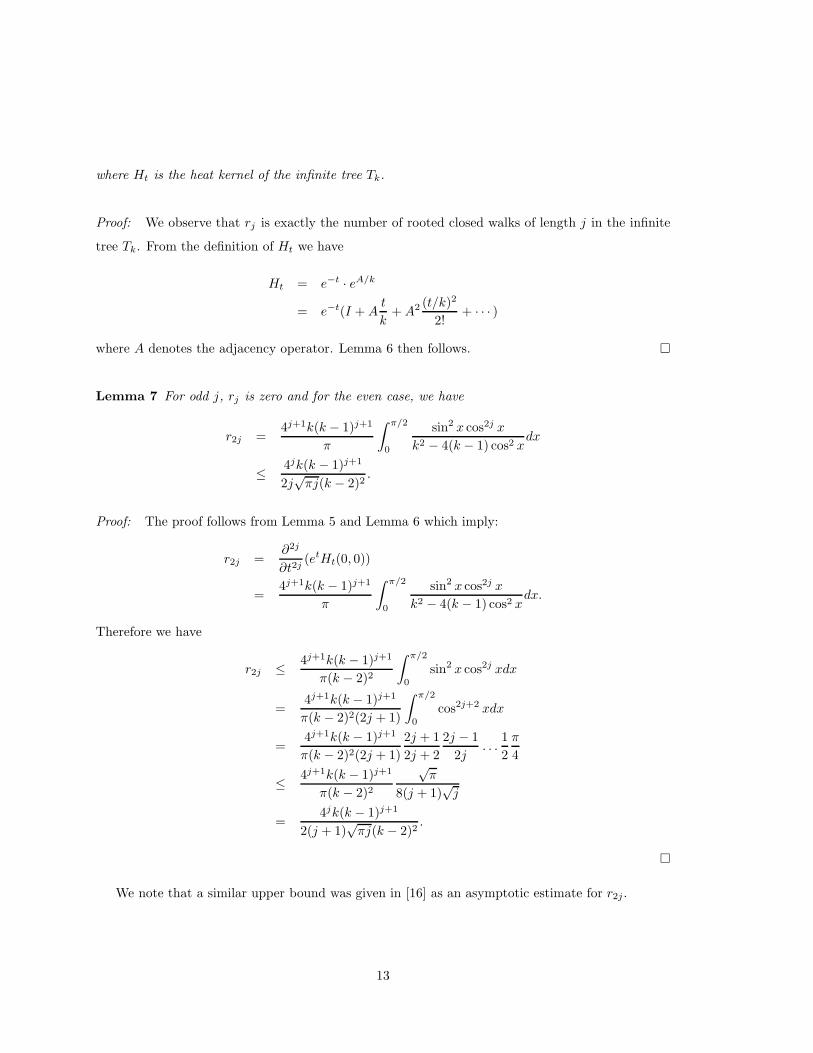
where Ht is the heat kernel of the infinite tree Tk.

Proof: We observe that rj is exactly the number of rooted closed walks of length j in the infinite

tree Tk. From the definition of Ht we have

Ht = e−t · eA/k

= e−t(I + At

k+ A2 (t/k)2

2!+ · · · )

where A denotes the adjacency operator. Lemma 6 then follows. �

Lemma 7 For odd j, rj is zero and for the even case, we have

r2j =4j+1k(k − 1)j+1

π

∫ π/2

0

sin2 x cos2j x

k2 − 4(k − 1) cos2 xdx

≤ 4jk(k − 1)j+1

2j√

πj(k − 2)2.

Proof: The proof follows from Lemma 5 and Lemma 6 which imply:

r2j =∂2j

∂t2j(etHt(0, 0))

=4j+1k(k − 1)j+1

π

∫ π/2

0

sin2 x cos2j x

k2 − 4(k − 1) cos2 xdx.

Therefore we have

r2j ≤ 4j+1k(k − 1)j+1

π(k − 2)2

∫ π/2

0

sin2 x cos2j xdx

=4j+1k(k − 1)j+1

π(k − 2)2(2j + 1)

∫ π/2

0

cos2j+2 xdx

=4j+1k(k − 1)j+1

π(k − 2)2(2j + 1)2j + 12j + 2

2j − 12j

. . .12

π

4

≤ 4j+1k(k − 1)j+1

π(k − 2)2

√π

8(j + 1)√

j

=4jk(k − 1)j+1

2(j + 1)√

πj(k − 2)2.

�

We note that a similar upper bound was given in [16] as an asymptotic estimate for r2j .

13

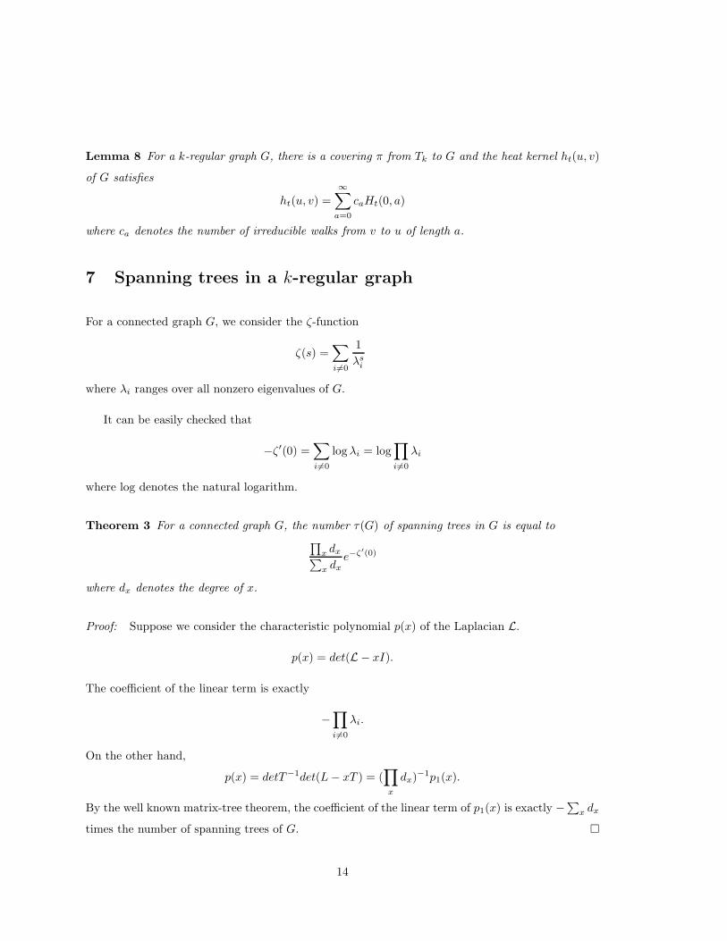
Lemma 8 For a k-regular graph G, there is a covering π from Tk to G and the heat kernel ht(u, v)

of G satisfies

ht(u, v) =∞∑

a=0

caHt(0, a)

where ca denotes the number of irreducible walks from v to u of length a.

7 Spanning trees in a k-regular graph

For a connected graph G, we consider the ζ-function

ζ(s) =∑i6=0

1λs

i

where λi ranges over all nonzero eigenvalues of G.

It can be easily checked that

−ζ′(0) =∑i6=0

log λi = log∏i6=0

λi

where log denotes the natural logarithm.

Theorem 3 For a connected graph G, the number τ(G) of spanning trees in G is equal to∏x dx∑x dx

e−ζ′(0)

where dx denotes the degree of x.

Proof: Suppose we consider the characteristic polynomial p(x) of the Laplacian L.

p(x) = det(L − xI).

The coefficient of the linear term is exactly

−∏i6=0

λi.

On the other hand,

p(x) = detT−1det(L − xT ) = (∏x

dx)−1p1(x).

By the well known matrix-tree theorem, the coefficient of the linear term of p1(x) is exactly −∑x dx

times the number of spanning trees of G. �

14

Thus, the number of spanning trees of a k-regular graph on n vertices satisfies

τ(G) =kn−1

ne−ζ′(0). (2)

In the rest of the paper, we assume that G is k-regular.

The trace function Tr ht of G satisfies

Tr ht =∑

i

e−tλi .

Therefore the zeta function satisfies

ζ(s) =1

Γ(s)

∫ ∞

0

ts−1(Tr ht − 1)dt (3)

by using the fact that1

Γ(z)

∫ ∞

0

e−ρttz−1dt =1ρz

. (4)

8 The maximum number of spanning trees in k-regular graphs

McKay [16] gave the following bounds for the maximum number of spanning trees over all k-regular

graphs Gn on n vertices:

c11n

Cn ≤ max τ(G) ≤ c2log n

nCn

where

C =(k − 1)k−1

(k2 − 2k)k/2−1

and c1 and c2 depend only on k ( in some complicated formula). He conjectured that the upper

bound is the right order for max τ(Gn). Here we will simplify the upper bound and prove that

indeed it is best possible within a constant factor.

Theorem 4 For k ≥ 3, the number τ(Gn) of spanning trees in a k-regular graph Gn on n vertices

satisfies

τ(Gn) ≤ (1 + o(1))2 logn

kn log k

((k − 1)k−1

(k2 − 2k)k/2−1

)n

.

Theorem 5 For k ≥ 8, there are k-regular graphs G on n vertices having the number τ(Gn) of

spanning trees satisfying

τ(G) ≥ (1 + o(1))log n

kn log k

((k − 1)k−1

(k2 − 2k)k/2−1

)n

.

15

We first need to establish the relation between the heat kernels ht and Ht. Let r′j denote the

total number of rooted closed walks of length j which are not totally reducible. We then have

Tr ht = e−t∑j≥0

(nrj + r′j)(t/k)j

j!

= nHt(0, 0) + e−t∑j≥0

r′j(t/k)j

j!.

From equation (3), we have

ζ(s) =: ζ0(s) + ζ1(s)

where

ζ0(s) =n

Γ(s)

∫ ∞

0

ts−1Ht(0, 0)dt

and

ζ1(s) =1

Γ(s)

∫ ∞

0

ts−1e−t

∑

j≥0

r′j(t/k)j

j!− et

.

We have

ζ0(s) =n

Γ(s)

∫ ∞

0

ts−1Ht(0, 0)dt

=2nk(k − 1)

πΓ(s)

∫ ∞

0

ts−1

∫ π

0

e−t(1− 2√

k−1k cos x) sin2 x

k2 − 4(k − 1) cos2 xdxdt

=2nk(k − 1)

π

∫ π

0

1

(1 − 2√

k−1k cosx)s

· sin2 x

k2 − 4(k − 1) cos2 xdx.

Therefore

ζ′0(0) = −2nk(k − 1)π

∫ π

0

sin2 x

k2 − 4(k − 1) cos2 xlog(1 − 2

√k − 1k

cosx)dx

= n logkk/2(k − 2)k/2−1

(k − 1)k−1. (5)

The above integral is evaluated by using the following formula given in [16]:

k

2π

∫ ω

−ω

(ω2 − x2)1/2

k2 − x2log(1 − γx)dx = − log

(η(

k − η

k − 1)k/2−1

)

where |γ| = 1/k < 1/ω, ω = 2√

k − 1 and η = 1−(1−4(k−1)γ2)1/2

2(k−1)γ2 .

16

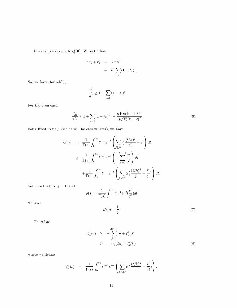
It remains to evaluate ζ′1(0). We note that

nrj + r′j = TrAj

= kj∑

i

(1 − λi)j .

So, we have, for odd j,

r′jkj

≥ 1 +∑i6=0

(1 − λi)j .

For the even case,

r′2j

k2j≥ 1 +

∑i6=0

(1 − λi)2j − n4jk(k − 1)j+1

j√

πj(k − 2)2. (6)

For a fixed value β (which will be chosen later), we have

ζ1(s) =1

Γ(s)

∫ ∞

0

ts−1e−t

∑

j≥0

r′j(t/k)j

j!− et

dt

≥ 1Γ(s)

∫ ∞

0

ts−1e−t

−

2β−1∑j=0

tj

j!

dt

+1

Γ(s)

∫ ∞

0

ts−1e−t

∑

j>2β

(r′j(t/k)j

j!− tj

j!)

dt.

We note that for j ≥ 1, and

ρ(s) =1

Γ(s)

∫ ∞

0

ts−1e−t(tj

j!)dt

we have

ρ′(0) =1j. (7)

Therefore

ζ′1(0) ≥ −2β−1∑j=1

1j

+ ζ′2(0)

≥ − log(2β) + ζ′2(0) (8)

where we define

ζ2(s) =1

Γ(s)

∫ ∞

0

ts−1e−t

∑

j≥2β

(r′j(t/k)j

j!− tj

j!)

.

17

Here, we have

ζ2(s) =1

Γ(s)

∫ ∞

0

ts−1e−t

∑

j≥2β

tj

j!

∑

i6=0

(1 − λi)j −∑j≥β

n4jk(k − 1)j+1

j√

πj(k − 2)2k2j

.

By using equation (7) and inequality (8), we have

ζ ′2(0) ≥∑j≥2β

∑i6=0

(1 − λi)j 1j−∑j≥β

n4jk(k − 1)j+1

j2√

πj(k − 2)2k2j

≥ −∑j≥β

n4jk(k − 1)j+1

j2√

πj(k − 2)2k2j

≥ −2n4βk(k − 1)β+1

β2√

πβ(k − 2)2k2β(9)

by using λi ≤ 2 and the fact that∑

j≥2β(1 − λi)j/j ≥ 0 .

Now, we are ready to prove Theorem 4 and 5.

Proof of Theorem 4:

From (2) and (5), we have

τ(G) =kn−1

ne−ζ′

0(0)−ζ′1(0)

=kn−1

n

((k − 1)k−1

kk/2(k − 2)k/2−1

)n

e−ζ′1(0)

=1kn

((k − 1)k−1

(k2 − 2k)k/2−1

)n

e−ζ′1(0). (10)

By using the preceding lower bounds of ζ′1 in (8), we have

τ(G) ≤ 2β

kn

((k − 1)k−1

(k2 − 2k)k/2−1

)n

e−ζ′2(0).

We now choose β as:

β = d log n

log k2

4(k−1)

e.

From (9), we have

ζ′2(0) ≥ −2n4βk(k − 1)β+1

β2√

πβ(k − 2)2k2β

≥ −2k(k − 1)

β2√

πβ(k − 2)2.

18

Therefore, we have

τ(G) ≤ 2β

kn

((k − 1)k−1

(k2 − 2k)k/2−1

)n

e−ζ′2(0)

≤ (1 + o(1))2 log n

kn log k

((k − 1)k−1

(k2 − 2k)k/2−1

)n

.

Theorem 4 is proved. �

Proof of Theorem 5:

For a graph with girth (the length of the smallest cycle) g, we can take β = bg/2c and we have

ζ1(s) =1

Γ(s)

∫ ∞

0

ts−1e−t

∑

j≥0

r′j(t/k)j

j!− et

dt

=1

Γ(s)

∫ ∞

0

ts−1e−t

−

g∑j=0

tj

j!

dt

+1

Γ(s)

∫ ∞

0

ts−1e−t

∑

j>g

(r′j(t/k)j

j!− tj

j!)

dt.

ζ′1(0) ≤ −g−1∑j=1

1j

+ ζ′2(0)

≤ − log g + ζ′2(0) (11)

where here we will need to use some known results on random k-regular graphs. Erdos and Sachs

[8] proved that with positive probability, say at least 1/2, there is a k-regular graph on n vertices

having girth g satisfying

g = (1 + o(1))log n

log k

as n approaches infinity. Friedman [10] showed that with probability approaches 1, the expected

number of irreducible walks cj(v) rooted at a vertex v of length j, for k ≥ 8, is

E(cj(v)) = k(k − 1)j−1(1n

+ Errn,j)

where

Errn,j = O

((ckj)c(

j2√

k

n1+√

k−1/2+

1kj/2

)

).

We note that in the original paper of Friedman, only the case for even k was treated. However, the

argument of counting irreducible “words” made of letters can be extended to counting walks on the

k-trees for odd k in a similar way.

19

The expected number of closed walks of length j satisfies (see [10])

kj

(1 + (n − 1)pj,0 +

j∑s=1

npj,sErrn,s

)

where pj,s is the probability that a random walk of length j reduces to an irreducible walk of size s.

Hence, the number r′j of not totally reducible walks of length j satisfies

E(r′jkj

) = 1 − pj,0 +j∑

s=1

npj,sErrn,s.

Since pj,s ≤ 2jk−j+s, we have

ζ2(s) =1

Γ(s)

∫ ∞

0

ts−1e−t

∑

j≥2β

(r′j(t/k)j

j!− tj

j!)

≤ 1Γ(s)

∫ ∞

0

ts−1e−t

∑

j≥2β

(t/k)j

j!2j

j∑s=0

k−j+s(cks)c(s2

√k2s

n√

k−1/2+

1(k − 1)s/2

)

.

Therefore,

ζ ′2(0) ≤∑j≥g

1j

j∑s=1

2jk−j+s(cks)c(s2

√k2s

n√

k−1/2+

1(k − 1)s/2

)

= o(1).

Using (10) and combining the preceding bounds , we have

τ(G) =1kn

((k − 1)k−1

(k2 − 2k)k/2−1

)n

e−ζ′1(0)

≥ g

kn

((k − 1)k−1

(k2 − 2k)k/2−1

)n

e−ζ′2(0)

≥ (1 + o(1))log n

kn log k

((k − 1)k−1

(k2 − 2k)k/2−1

)n

.

This completes the proof of Theorem 5. �

References

[1] C. T. Benson, Minimal regular graphs of girth eight and twelve, Canad. J. Math. 18 (1996),

1091-1094.

[2] N. Biggs, Algebraic Graph Theory, Cambridge University Press, 1993.

20

[3] R. Brooks, The spectral geometry of k−regular graphs, Journal D’analyse Mathematrique, 57

(1991) 120-151.

[4] J. Cheeger and S.-T. Yau, A lower bound for the heat kernel, Communications on Pure and

Applied Mathematics XXXIV (1981), 465-480.

[5] D. M. Cvetkovic, M. Doob and H. Sachs, Spectra of graphs, Academic Press, New York, 1980.

[6] F. R. K. Chung and S.-T. Yau, A combinatorial trace formula, Tsing Hua Lectures on Geometry

and Analysis, (ed. S.-T. Yau), International Press, Cambridge, Massachusetts, 1997, 107-116.

[7] F. R. K. Chung, Spectral Graph Theory, CBMS Lecture Notes, 1997 , AMS Publication.

[8] P. Erdos and H. Sachs, Regulare Graphen gegenebener Teillenweite mit Minimaler Knotenzahl,

Wiss. Z. Univ. Halle – Wittenberg, Math. Nat. R. 12 (1963), 251-258.

[9] W. Feit and G. Higman, The non-existence of certain generalized polygons, J. Algebra 1 (1964),

114-131.

[10] J. Friedman, On the second eigenvalues and random walks in random d-regular graphs, Com-

binatorica 11 (1991), 331-362.

[11] A. K. Kelmans, On properties of the characteristic polynomial of a graph, Kibernetiku-Na Sluzbu

Kommunizmu 4 Gosenergoizdat, Moscow, 1967.

[12] C. D. Godsil and B. D. McKay, Feasibility conditions for the existence of walk-regular graphs,

Linear Algebra Appl., 30 (1980), 51-61.

[13] F. Kirchhoff, Uber die Auflosung der Gleichungen, auf welche man bei der Untersuchung der

linearen Verteilung galvanischer Strome gefuhrt wird, Ann. Phys. chem. 72 (1847) 497-508.

[14] B. D. McKay, Backtrack programming and the graph isomorphism problem, M. Sc. Thesis,

University of Melbourne, 1976.

[15] B. D. McKay, The expected eigenvalue distribution of a large regular graph, Linear Algebra

and its Applications 40 (1981), 203-216.

[16] B. D. McKay, Spanning trees in regular graphs, Europ. J. Combinatorics 4 (1983), 149-160.

[17] Peter Sarnak, Some Applications of Modular Forms, Cambridge University Press, New York,

1990.

21

[18] Richard M. Schoen and S.-T. Yau, Lectures on Differential Geometry, International Press,

Cambridge, Massachusetts, 1994.

[19] R. R. Singleton, On minimal graphs of maximum even girth, J. Comb. Th 1 (1966), 306-322.

22