NBER WORKING PAPER SERIES

COVID-19 AND EMERGING MARKETS:A SIR MODEL, DEMAND SHOCKS AND CAPITAL FLOWS

Cem ÇakmaklıSelva Demiralp

Ṣebnem Kalemli-ÖzcanSevcan Yesiltas

Muhammed A. Yildirim

Working Paper 27191http://www.nber.org/papers/w27191

NATIONAL BUREAU OF ECONOMIC RESEARCH1050 Massachusetts Avenue

Cambridge, MA 02138May 2020, Revised June 2021

This paper is previously circulated under the title: “An Epidemiological Multi-Sector Model for a Small Open Economy with an Application to Turkey.” We would like to thank webinar participants at London School of Economics, Central Bank of Chile, EU Delegation in Ankara, and Koc¸ Holding for their valuable feedback. The views expressed herein are those of the authors and do not necessarily reflect the views of the National Bureau of Economic Research.

NBER working papers are circulated for discussion and comment purposes. They have not been peer-reviewed or been subject to the review by the NBER Board of Directors that accompanies official NBER publications.

© 2020 by Cem Çakmaklı, Selva Demiralp, Ṣebnem Kalemli-Özcan, Sevcan Yesiltas, and Muhammed A. Yildirim. All rights reserved. Short sections of text, not to exceed two paragraphs, may be quoted without explicit permission provided that full credit, including © notice, is given to the source.

COVID-19 and Emerging Markets: A SIR Model, Demand Shocks and Capital Flows Cem Çakmaklı, Selva Demiralp, Ṣebnem Kalemli-Özcan, Sevcan Yesiltas, and Muhammed A. YildirimNBER Working Paper No. 27191May 2020, Revised June 2021JEL No. E01,F23,F41

ABSTRACT

We quantify the macroeconomic effects of COVID-19 for a small open economy in the absence of vaccinations. We use a framework that combines a multi-sector SIR model with data on international and inter-sectoral trade to estimate the effects of a joint collapse in domestic and foreign demand. We calibrate our framework to Turkey and estimate the COVID-19 related output losses for each sector. Domestic infection rates feed directly into sectoral demand shocks, where sectoral supply is affected both from sick workers and lockdowns. Sectoral demand shocks additionally capture foreign infection rates through foreign demand. We use real-time credit card purchases to pin down the magnitude of these domestic and foreign demand shocks. Our results show that the optimal policy, which yields the lowest economic cost and saves the maximum number of lives, can be achieved under an early and globally coordinated full lockdown of 39 days, amounting to a loss of 5.8 percent of GDP in the small open economy. To illustrate the importance of foreign demand, we compare the economic costs under globally coordinated vs. uncoordinated lockdown scenarios and incorporate the role of fiscal stimulus packages. Our findings illustrate that the economic drag in the rest of the world due to ineffective lockdown measures increases the economic toll in the small open economy by up to 2 percent of GDP. Meanwhile the stimulus packages abroad, by increasing foreign demand for small open economy’s goods, reduce costs by 0.5 percentage points. We further show that the lack of a similar large fiscal package in the small open economy can be remedied by capital inflows into sectors with large losses.

Cem ÇakmaklıKoç University College of Administrative Sciences and Economics Rumelifener YoluSariyer, IstanbulTurkeyccakmakli@ku.edu.tr

Selva DemiralpKoç UniversityRumelifeneri Yolu, Sariyer Istanbul 34450Turkeysdemiralp@ku.edu.tr

Ṣebnem Kalemli-ÖzcanDepartment of Economics University of Maryland Tydings Hall 4118DCollege Park, MD 20742-7211 and CEPRand also NBER kalemli@econ.umd.edu

Sevcan YesiltasKoç UniversityDepartment of Economics and FinanceRumelifeneri Yolu 34450 Sariyer, Istanbul Turkeysyesiltas@ku.edu.tr

Muhammed A. YildirimKoç University and Center for International Development at Harvard University mayildirim@ku.edu.tr

“Best safety lies in fear.”

– William Shakespeare

1 Introduction

The COVID-19 pandemic has the potential to trigger the biggest emerging market (EM) crises of

modern times. At the onset of the pandemic, EMs observed a collapse in domestic and external de-

mand, capital outflows, and depreciating currencies. Although the capital flows came back thanks

to the ultra expansionary monetary policies of the major central banks, domestic and external de-

mand are not fully back to pre-pandemic levels in emerging markets. With the extensive fiscal

stimulus and the vaccine-led recovery in the advanced countries, notably the U.S., many argued

that emerging markets can turn the corner as a result of the increase in demand for their goods from

the advanced countries (OECD, 2021).

To understand the positive spillover effects of an increase in foreign demand, while emerging

markets are still battling the pandemic, we first need to understand the macroeconomic effects of the

original collapse in domestic and foreign demand as a result of the health shock. To do so, we utilize

an epidemiological Susceptible-Infected-Recovered (SIR)- multi-sector-macro model to calculate the

sector level output losses for a small open economy. We then evaluate the optimal lockdown policy

to avoid these losses by calibrating our model to Turkey.1

The key properties of our framework are as follows. On the demand side, our model contains a

domestic component and a foreign component for sectoral demand shocks. Both types of demand

decline as the infections increase in the home country and foreign country, where the lowest demand

is calibrated using real time sector-level credit card purchases. The supply shock is purely domestic,

as a function of sick workers and lockdowns. In order to filter out the role of foreign demand,

we compare the costs under a globally coordinated full lockdown against an uncoordinated full

lockdown. In the case of a globally coordinated full lockdown, all countries suffer from supply

and demand shocks in a synchronized manner. In the case of an uncoordinated full lockdown, we

assume that Turkey implements a full lockdown while its trade partners implement either a full or

1See Cakmakli et al. (2020) for the earlier working paper version of our model, April (2020).

2

a partial lockdown. The increase in estimated costs in the case of an uncoordinated full lockdown

reflects the additional decline in foreign demand due to the rise in the number of cases as a result

of partial lockdown in these trading partners. The consequent decline in demand in these countries

is reflected as a decline in the export revenue for Turkey. In a similar vein, adoption of stimulus

packages in the rest of the world reduces the economic costs in Turkey due to improvement in

demand for Turkish exports.

There will be sectoral heterogeneity both in the supply and demand shocks. For the supply side,

heterogeneity will depend on the ability to work from home and physical proximity needed for the

job. Demand shocks are also heterogeneous across sectors given the strength of foreign demand for

a sector’s output and the fluctuations in domestic demand based on consumer preferences that de-

pend on infections. Our methodology is for the short run, where the output is demand determined

with fixed prices.

Our approach has the advantage of being simple and easily mapped to real time data. The

model is calibrated to Turkey by using Turkey’s international linkages to 65 other countries through

35 sectors. We use international input-output (I-O) linkages to measure the foreign demand for each

of the domestic sectors’ output. We show that, almost 30 percent of the sectoral economic costs for

Turkey stem from lower foreign demand in a coordinated full lockdown. Our work differs starkly

from the COVID-19 literature that put the epidemiology at the center but focus mostly on closed

economies.2 Considering an open economy framework allows us to incorporate the role of global

coordination, or lack thereof, in determining the effectiveness of lockdown measures.

Contrary to the popular belief that no lockdown policies would minimize economic costs, we

show that such policies are actually costlier than an effective full lockdown given the importance

of domestic and external demand shocks. If the lockdown is globally coordinated, the costs of a

full lockdown are further minimized by containing the pandemic at the global scale and preventing

future waves. Our findings are consistent with the findings of Goolsbee and Syverson (2020) for the

US, who shows that, using real time data, legal shutdown orders account for only a modest share of

the decline of economic activity. Data on real GDP growth in 2020 further support our predictions.

2The two exceptions that highlight the open economy dimension are Arellano et al. (2020) who focus on sovereigndefault risk under COVID shock with a SIR and sovereign debt model; and Antras et al. (2020), who analyze the interplaybetween globalization and pandemic via trade-induced personal interactions.

3

The countries that imposed early and strict lockdowns such as China, Australia, and New Zealand

experienced earlier economic normalization 2020 compared to the rest of the world.3 In general,

countries that implemented full and effective lockdowns at an early stage saved more lives and

minimized the economic costs at the same time, a result that our model generates.

Our model based estimate for the total cost of containing the pandemic immediately, with an

early and strict lockdown is about 5.8 percent of the GDP (at an annualized rate). This implies that

output declines by 17.5 percent during the quarter in which the lockdown is imposed, compared to

the previous quarter. The optimal lockdown lasts 39 days. Demand normalizes after the lockdown,

and the economy returns to normal during the rest of the year, smoothing out the shock. Under no

lockdown, the cost of the pandemic increases from 5.8 to 11 percent of GDP annually. The reason for

the increase is that, under no lockdown (or partial lockdown), even though businesses remain open,

there are still interruptions in supply as people get infected, and demand declines due to voluntary

social distancing measures. Demand particularly declines for those sectors where the possibility

of getting infected is higher such as travel or restaurants. In general, sectors that are most severely

affected from the pandemic are those that are either (i) closed due to lockdown measures, (ii) observe

a collapse in demand due to close proximity requirements, or (iii) more exposed to international

spillovers through trade linkages.

We consider several experiments to underline the role of global coordination and its implications

on external demand. If the full lockdown is not globally coordinated and the rest of the world

implements partial lockdown while Turkey implements full lockdown, then the costs that are borne

by Turkey increase from 5.8 percent to 7.8 percent of GDP. If 50 percent of the countries in the world

implement full lockdown together with Turkey, then the costs are estimated to be 6.9 percent of

Turkish GDP. The key message from this exercise is that, even if a small open economy implements

the most strict full lockdown and eliminates the pandemic at home, it will bear further costs through

a decline in foreign demand if the rest of the world does not cooperate. When the pandemic prolongs

in the outside world, then it will reduce the exports of the country that contains the virus within its

borders.

Several closed economy papers employing epidemiological models similar to us, including Ace-

3https://www.imf.org/external/datamapper/NGDP RPCH@WEO/OEMDC/ADVEC/WEOWORLD

4

moglu et al. (2020), Alvarez et al. (2020), Farboodi et al. (2020), and Eichenbaum et al. (2020) reach

comparable conclusions. Accordingly, imposing full lockdowns or stricter measures at the early

stages of the pandemic lower economic costs by normalizing aggregate demand sooner. We argue

that, for an open economy, the superiority of a coordinated full lockdown over a partial lockdown is

even bigger. This is because demand will be lower in the absence of a full lockdown abroad, which

amplifies the domestic demand shock via sectoral I-O linkages.4

The heterogeneity in infection rates by the job type and age are critical in our framework as this

heterogeneity will deliver the sectoral heterogeneity in terms of output losses. In no lockdown sce-

nario, most of the population is fully exposed to the outbreak. Nevertheless, the working population

is under higher risk compared to the non-working population. In partial lockdown scenario, tele-

workable occupations start working from home and hence the base infection rate declines for this

group. It is important to note that the individuals in the highest risk group, ages 65 and above, as

well as the younger people are assumed to have lower infection rates because they do not work or

because they switch to distanced learning. This is consistent with the optimal setting identified by

Acemoglu et al. (2020). The infection rate is still high for the on-site workers. In full lockdown, we

assume that only the essential sectors require their non-teleworkable employees on-site. This is why

the infection rate declines substantially for the remainder of the population that stays home under

full lockdown and therefore normalizing the demand.

Our benchmark estimates of economic costs are in the absence of any policy action. Costs might

decline when fiscal and monetary policy responses are taken into consideration. We prefer to pro-

vide our baseline estimates based on no policy action so that the minimum magnitude of the fiscal

policy packages can be identified. This approach makes our findings particularly relevant under the

threat of multiple waves after reopening. If the economy opens up prematurely, the increase in the

number of infections would stall demand again, even if the businesses remain open. The consequent

economic costs may lead to lasting economic damage by extending the duration of the recession. In-

4In our follow-up paper we illustrate an even bigger amplification mechanism once international production linkagesare incorporated into our model on top of the final good trade linkages that we have here. In that framework, a supplyshock in one country can affect all its trading partners through trade in intermediate inputs. In a model with no infectiondynamics (SIR), Baqaee and Farhi (2020a) exploit nonlinear production networks in a general equilibrium framework andshow that non-linearities amplify the impact of COVID-19 between 20 to 100 percent. See also Baqaee and Farhi (2020b).The work by Guerrieri et al. (2020) does not include an infection dynamics model either but underlines the importance ofa multi-sector economy, where supply shocks can turn into larger aggregate demand shocks.

5

deed, if the lockdown ends prematurely, we show that the duration of a lockdown that is needed to

contain the virus increases to more than one year.5

Last but not least, we evaluate the role of fiscal policy and show that capital flows can make up

for the limited domestic fiscal packages in emerging markets. We illustrate that sectors with stronger

international connections suffer more from the pandemic due to a significant decline in external

demand. Such costs are positively associated with the absence of effective lockdown measures in

the trading partners, but negatively associated with large fiscal stimulus packages in these same

trading partners. We show that capital inflows into sectors with large losses are particularly effective

in mitigating those losses under a coordinated global lockdown.

We organize the remainder of the paper as follows: Section 2 describes the literature. In Section

3, we briefly go over the background for Turkey. Section 4 describes the model. Section 5 presents

our quantitative results. Section 6 concludes.

2 COVID-19 Literature and Our Contribution

The literature on understanding the economic impact of COVID-19 pandemic has resulted in an

ever-growing list of papers. To capture the infection dynamics, many studies use SIR models or

its extensions. Papers such as Stock (2020) and Alvarez et al. (2020) consider a standard SIR model

and focus on the trade off between unemployment that arises from lockdowns versus the number

of deaths due to the pandemic. They reach the conclusion that the optimal policy is a full lockdown

that covers the majority of the population where the restrictions are removed gradually afterwards.

Acemoglu et al. (2020) consider a multi-risk SIR model by focusing on the structural differences in

the severity of infections for distinct age groups that affect lockdown policies and economic costs.

They show that targeted measures such as full lockdown for the elderly group could be more ef-

fective. Alon et al. (2020) also consider a closed economy model but approaches the problem from

the developing country perspective, considering market distortions and the presence of an informal

sector and hand to mouth consumers. They realize that such economies cannot fully lockdown and

5See https://www.thelancet.com/journals/lanpub/article/PIIS2468-2667(20)30073-6/fulltext, that argues that re-opening too soon before the R number is below 1 might trigger another peak. The case of Singapore is an example with re-curring lockdowns: https://www.theguardian.com/world/2020/apr/21/singapore-coronavirus-outbreak-surges-with-3000-new-cases-in-three-days

6

argue that lockdowns on the elderly population might be better.

Combining supply and demand in a SIR framework Farboodi et al. (2020) internalize the indi-

vidual choices for social distancing and study both laissez-faire and social optimum scenarios. They

find that even in the laissez-faire case individuals choose to sharply reduce their activity but the

socially optimal response imposes severe restrictions at the onset of the outbreak. Eichenbaum et al.

(2020) incorporate supply and demand in a SIR model as well, where the government is assumed

to alter the individuals’ activities through a consumption tax and again find that relatively severe

containment at the beginning of the pandemic is the most socially optimum response. Krueger et

al. (2020) extends the model by Eichenbaum et al. (2020) and introduces differential transmission

rates based on the consumption or employment choice. They aim to capture the interplay between

infection dynamics and the demand side or the supply side –but not both of them simultaneously.

The above cited literature do not feature sectoral heterogeneity for demand and supply shocks

together. However, the pandemic evidence shows the magnitude of the demand shock to be very

large and vary by sector, as we model. Specifically, using granular data, Chetty et al. (2020) analyzed

the consumer spending during the first month of the pandemic in the United States and found that

the spending declined by 39% for consumers in the top-quartile and 13% in the bottom quartile of

the income distribution. The observed decline exhibits heterogeneity across sectors, with drastic

decreases in industries requiring in-person interactions.

Our paper is unique in combining supply and demand shocks at the sectoral level with a SIR

model for an open economy. Our open economy framework makes the role of global coordination

clear. If the lockdown can be implemented with global synchronization, the pandemic will be con-

trolled faster. As the number of infections decline globally, demand returns to pre-pandemic levels

faster as both domestic and foreign demand normalize sooner.

3 Background: Turkey

This section summarizes the economic environment in Turkey before the pandemic to provide a

background on initial conditions.

7

Since 2017, the inflation rate had been on the rise while Turkish Lira (TL) depreciated. Triggered

by the political tension between Turkey and US, August 2018 marked the beginning of an exchange

rate crisis, where rapidly depreciating TL brought many companies with FX debt to the edge of

bankruptcy. The significant decline in economic growth led to an improvement in the current ac-

count deficit because Turkey’s production heavily relies on imports of intermediary goods. The

growth rate in the first quarter of 2020 reached 4.5 percent and the unemployment rate declined to

12.7 percent.

Capital outflows by non-residents during COVID-19 led to a wave of depreciation in TL, which

required FX interventions and brought FX reserves to low levels. As of June 11, 2021, net reserves

of Central Bank of the Republic of Turkey (CBRT) stood at $14.9 billion. IMF-defined budget deficit

that excludes one-time transfers stands close to 5 percent of GDP while the current account deficit is

around 2.5 percent of GDP, as an average over the last 5 years.

Figure 1: External Debt and Currency Decomposition

(a) Decomposition in terms of Ownership30

40

50

60

70

Exte

rnal

10

15

20

25

30

35

40

1996

1997

1998

1999

2000

2001

2002

2003

2004

2005

2006

2007

2008

2009

2010

2011

2012

2013

2014

2015

2016

2017

2018

2019

2020

Public Private External

(b) Currency Decomposition

57

38

5

02

04

06

0

USD Other TL

NOTES: (a) This panel plots external debt (right x-axis) alongside with its public-private composition (left x-axis) forTurkey. Debt values are expressed as percentage of GDP. (b) This panel shows the currency composition of total externaldebt as of December 2020. Source: Turkey Data Monitor

Turkey relies heavily on capital flows to finance its external debt, which stood at 63 percent of

8

GDP at the end of 2020. Figure 1a shows the changes in the composition of external debt over time.

In 2001, total external debt was 57 percent of GDP. Of this, public sector debt was 24 percent, while

the private sector debt was 22 percent.6 After the 2001 crisis, external debt was reduced at first, but

it gradually built up in the years that followed. By the time we reached 2019, total external debt was

once again comparable to 2001 levels with 56 percent of the GDP. Different from 2001, however, this

time the lion’s share was held by the private sector debt which was 36 percent of the GDP while

the public debt was 21 percent of GDP. Another interesting pattern that is observed in Figure 1a is

the increasing trend in public borrowing in the period after 2012. As of December 2020, almost 60

percent of total external debt is denominated in USD (see Figure 1b).

4 The Framework

In this section, we develop a model that illustrates how COVID-19 affects the economy. We illustrate

that despite the increasing costs due to business closures, a full and coordinated lockdown contains

the virus in the fastest way. As we compare the recovery paths with and without the lockdown, we

observe that a full lockdown lasts for approximately 40 days while partial lockdown cannot contain

the virus within a year. Because the duration of the lockdown increases substantially, the economic

costs of a partial lockdown are significantly higher than full lockdown. The mortality numbers

present a stark contrast across alternative scenarios as well. Full lockdown, which has the lowest

economic costs also stands out as the best option that minimizes the number of deaths. Only 0.002

percent of the population dies in a well implemented full lockdown whereas the numbers range

between 0.32 to 0.96 percent in the case of partial lockdown. In the model we do not quantify the

economic costs of lost lives (see e.g., Greenstone and Nigam (2020)) under alternative lockdown

scenarios. Had we incorporated the costs of deaths, the superiority of full lockdown would be even

more striking.

6The sub-components do not add up because the remainder of the external debt is held by CBRT.

9

4.1 The SIR Model for Pandemic

We use the workhorse model of the pandemic, the Susceptible-Infected-Recovered (SIR) model,

which has been heavily used in epidemiology (see Allen (2017) for a primer). According to this

model, the population (denoted by N) can be split into three disjoint groups, namely the Susceptible

(St), Infected (It) and Recovered (Rt) individuals at any time t. The individuals in the suscepti-

ble group can contract the disease from the individuals in the infected group. Those who develop

immunity to the disease (either by going through the disease or by vaccination) constitute the re-

covered group. At any given time, the number of susceptible individuals decreases and the number

of people in the recovered group increases. The severity of the pandemic is related to the size of the

infected group. We quantify the progression of the pandemic using certain assumptions. An inter-

action between a susceptible and an infected individual can occur with a probability proportional

to St × It/N, where N serves as the normalization constant. The disease would be transmitted with

a ratio of β during this interaction. On the other hand, among the infected individuals, a ratio γ

recovers from the disease.7 Combining these ideas into a mathematical formulation, we arrive at the

following equations that govern the law of motion of the pandemic at any given time:

∆St = −βSt−1It−1

N

∆Rt = γIt−1

∆It = βSt−1It−1

N− γIt−1 (1)

Since St + It + Rt + N, the summation of the differences, i.e., ∆St + ∆Rt + ∆It = 0, is always zero.

Conventional SIR models treat interactions between the individuals as homogeneous. In real

life, however, interaction patterns exhibit a great degree of variation among different industries. For

instance, a dentist needs to work in close proximity to others to perform her job whereas a computer

programmer does not require physical proximity. Because each industry employs a variety of occu-

pations, the physical proximity requirements of occupations would create sectoral heterogeneity in

different work-spaces. In turn, this sectoral heterogeneity leads to different infection dynamics and

7We do not model mortality here. Please see Atkeson (2020), Bendavid and Bhattacharya (2020), Dewatripont et al.(2020), Fauci et al. (2020), Li et al. (2020), Linton et al. (2020), and Vogel (2020) for models with mortality.

10

trajectories. We assume that the industries that require a greater degree of physical proximity would

be more prone to infections.8

We incorporate the heterogeneity in infection dynamics stemming from sectoral composition

into the SIR model. First, we distinguish between working and non-working populations, where

the latter is denoted by NNW . We assume that the economy consists of K sectors, which are indexed

by i = 1, . . . , K, each with Li workers. During the pandemic, if a worker can do her job remotely, she

does not need to show up to the work site. We classify these workers as ”teleworkable.” We calculate

the teleworkable share of employment from Dingel and Neiman (2020)’s list of teleworkable occu-

pations. The remaining workers need to be on-site to fulfill their tasks. The number of teleworkable

employees in industry i is denoted by TWi and on-site workers are denoted by Ni, such that:

Li = TWi + Ni. (2)

In terms of disease susceptibility, teleworkable employees and non-working population can be

lumped together because they are both assumed to be ”at-home.” We use i = 0 to represent the

at-home group where the size of this group is:

N0 = NNW +K

∑i=1

TWi. (3)

We assume that the at-home group is the least susceptible group and has an infection rate of β0.

Being at the job site increases the risk of contracting the disease and this increase is intimately related

to the hetereogenity of physical proximity requirements of industries. Therefore, we define the

infection rate within industry i to be:

βi = β0Proxi for i = 1, . . . , K (4)

where Proxi captures the proximity requirement of industry i. We calculate the physical proximity

requirements for occupations using the O*NET dataset (see Section 5.1 for details). One caveat with

this approach is that during the pandemic the physical proximity requirements of industries could

8 In a report analyzing the effects of the pandemic on its members, DISK labor union in Turkey claims that the infectionrate increases three times among workers compared to rest of the society: http://disk.org.tr/2020/04/rate-of-covid-19-cases-among-workers-at-least-3-times-higher-than-average/

11

be adjusted downwards (Eichenbaum et al., 2020). Here, we do not endogenize this decision in our

model and consider the proximity measure as exogenous.

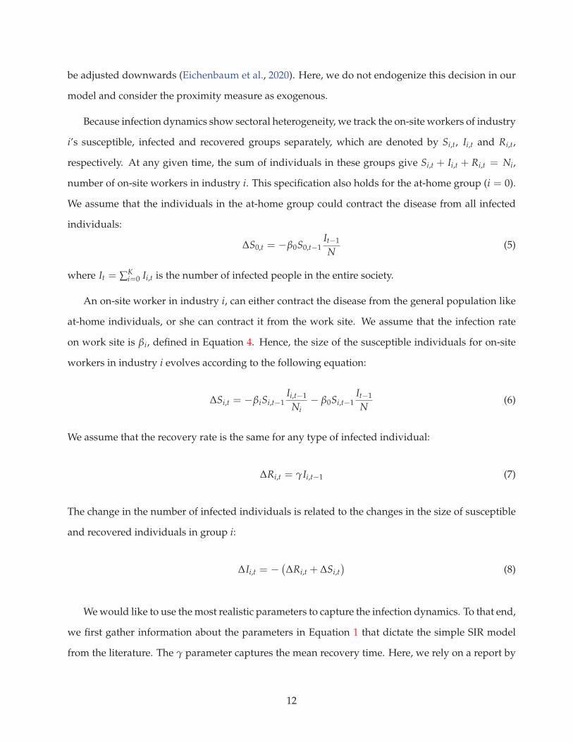
Because infection dynamics show sectoral heterogeneity, we track the on-site workers of industry

i’s susceptible, infected and recovered groups separately, which are denoted by Si,t, Ii,t and Ri,t,

respectively. At any given time, the sum of individuals in these groups give Si,t + Ii,t + Ri,t = Ni,

number of on-site workers in industry i. This specification also holds for the at-home group (i = 0).

We assume that the individuals in the at-home group could contract the disease from all infected

individuals:

∆S0,t = −β0S0,t−1It−1

N(5)

where It = ∑Ki=0 Ii,t is the number of infected people in the entire society.

An on-site worker in industry i, can either contract the disease from the general population like

at-home individuals, or she can contract it from the work site. We assume that the infection rate

on work site is βi, defined in Equation 4. Hence, the size of the susceptible individuals for on-site

workers in industry i evolves according to the following equation:

∆Si,t = −βiSi,t−1Ii,t−1

Ni− β0Si,t−1

It−1

N(6)

We assume that the recovery rate is the same for any type of infected individual:

∆Ri,t = γIi,t−1 (7)

The change in the number of infected individuals is related to the changes in the size of susceptible

and recovered individuals in group i:

∆Ii,t = −(

∆Ri,t + ∆Si,t

)

(8)

We would like to use the most realistic parameters to capture the infection dynamics. To that end,

we first gather information about the parameters in Equation 1 that dictate the simple SIR model

from the literature. The γ parameter captures the mean recovery time. Here, we rely on a report by

12

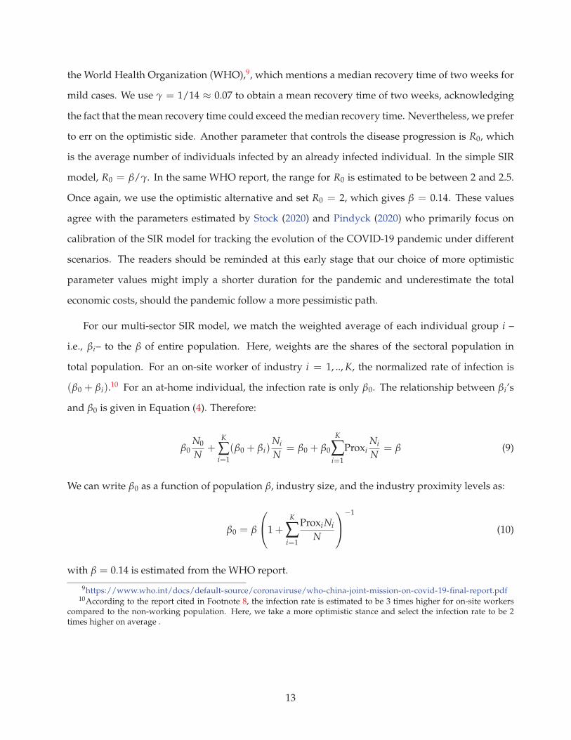
the World Health Organization (WHO),9, which mentions a median recovery time of two weeks for

mild cases. We use γ = 1/14 ≈ 0.07 to obtain a mean recovery time of two weeks, acknowledging

the fact that the mean recovery time could exceed the median recovery time. Nevertheless, we prefer

to err on the optimistic side. Another parameter that controls the disease progression is R0, which

is the average number of individuals infected by an already infected individual. In the simple SIR

model, R0 = β/γ. In the same WHO report, the range for R0 is estimated to be between 2 and 2.5.

Once again, we use the optimistic alternative and set R0 = 2, which gives β = 0.14. These values

agree with the parameters estimated by Stock (2020) and Pindyck (2020) who primarily focus on

calibration of the SIR model for tracking the evolution of the COVID-19 pandemic under different

scenarios. The readers should be reminded at this early stage that our choice of more optimistic

parameter values might imply a shorter duration for the pandemic and underestimate the total

economic costs, should the pandemic follow a more pessimistic path.

For our multi-sector SIR model, we match the weighted average of each individual group i –

i.e., βi– to the β of entire population. Here, weights are the shares of the sectoral population in

total population. For an on-site worker of industry i = 1, .., K, the normalized rate of infection is

(β0 + βi).10 For an at-home individual, the infection rate is only β0. The relationship between βi’s

and β0 is given in Equation (4). Therefore:

β0N0

N+

K

∑i=1

(β0 + βi)Ni

N= β0 + β0

K

∑i=1

ProxiNi

N= β (9)

We can write β0 as a function of population β, industry size, and the industry proximity levels as:

β0 = β

1 +K

∑i=1

ProxiNi

N

−1

(10)

with β = 0.14 is estimated from the WHO report.

9https://www.who.int/docs/default-source/coronaviruse/who-china-joint-mission-on-covid-19-final-report.pdf10According to the report cited in Footnote 8, the infection rate is estimated to be 3 times higher for on-site workers

compared to the non-working population. Here, we take a more optimistic stance and select the infection rate to be 2times higher on average .

13

4.2 Production

We specify a simplified version of the production function where output is a linear function of labor.

This treatment emphasizes the impact of the pandemic on production through changes in labor

supply. Here, we implicitly assume that the amount of the capital stock remains the same in the

short-run, and therefore, can be omitted during normal times as well as the pandemic period. We

model production as a function of the number of workers in industry i as:

Yi = ZiLi (11)

where Zi denotes the productivity of workers in sector i.

During the pandemic period, the level of production decreases because the infected individuals

cannot work until they recover from the disease. For each industry i, we have two groups of workers,

teleworkable, whose size is TWi and on-site, with size Ni. The number of infected individuals among

on-site workers is Ii,t. Teleworkers are considered to be as a part of at-home group, whose size is N0

with active infections of I0,t. Hence, the total number of available workers at time t will be:

Li,t = (Ni − Ii,t) + TWi

(

1 −I0,t

N0

)

(12)

Since we assume a linear production function, the output in industry i decreases due to the ongoing

pandemic with the levels at:

YSi,t = Zi Li,t = Yi

Li,t

Li. (13)

4.3 Demand

During the pandemic, the daily routines and priorities change drastically to avoid the risk of getting

infected. This voluntary social distancing, or put differently, the “fear” of getting infected, leads to

substantial changes in consumer preferences. This is true both for domestic and foreign demand.

The demand channel allows us to incorporate the role of global coordination by focusing on how

lockdown decisions in a country’s trade partners affect the demand for its exports.

The changes in preferences evolve as the pandemic progresses. We assume that the demand tran-

14

sitions from the “normal” to a worst case scenario during the brunt of the pandemic. Specifically,

we consider two demand profiles, representing the normal times and the turbulent times. To cali-

brate these profiles, we track the consumption data from the national accounts and the credit card

spending data. While the first dataset is of low frequency and published with a delay, the latter is

available at the weekly frequency. Therefore, it provides us with useful information on the changes

in demand structure over the course of pandemic. We complement the credit card data with sector

specific information in industry reports and expert opinions if the spending in a sector is not often

done with credit cards.11 We specify a smooth function that transition gradually between these two

demand profiles depending on the number of infections. After determining demand, we use the

input-output framework and map the final good consumption, both domestic and foreign, back to

output in each industry.

In modeling the demand side in terms of the domestic and foreign demands, we assume that

for a country c = 1, ...., C, a representative agent allocates her income optimally among different

final goods, by maximizing her utility function through expenditures on these goods. Here, we

use a Cobb-Douglas specification for the utility function of the representative agent in line with the

literature on input-output analysis (e.g., Acemoglu et al. (2012), among others). Specifically, we use

the following utility function:

U(e1, . . . , en) =n

∏i=1

eαii , (14)

where ei is the expenditure on the final good of industry i and αi refers to industry i’s share in total

expenditure together with ∑ni=1 αi = 1 and 0 < αi < 1∀i = 1, . . . , n. As a natural consequence of the

Cobb-Douglas formulation, αi represents the share of expenditures on the final good i in the budget

of the representative agent. Suppose that the income (wage) of the representative agent is w. Then

the expenditure in industry i can be written as ei = αiw.

The pandemic alters the demand profile and expenditure shares in each country. We assume

that demand is affected through two distinct channels during the pandemic. The first channel is the

effect of the pandemic on the priorities, and thus, on preferences. In this case, the sectoral weights

in the budget change following the changes in preferences. The utility function changes with the

11We present these demand changes and related data resources in Table A.3 of the Appendix.

15

weights as follows:

U(e1, . . . , en, Ic) =n

∏i=1

eαi(Ic)i , (15)

where the Cobb-Douglas exponents depend on the number of infections in each country, denoted

as Ic for c = 1, ..., C. αi(Ic) = αi for a small number of infections, i.e., Ic ≤ 0.1 Ic, where I is a scaling

parameter for infections. In the Turkish context, we set Ic to 50,000 to capture a relevant range for

the number of infections (see below for our simulations). Likewise, in the international case we set

Ic proportional to 50,000 with proportionality computed as the ratio of the population of the foreign

country to the population of Turkey. This limit implies that the utility function returns to normal

times if the number of infections remain below 5,000 (in the Turkish case). For large Ic, the limit

level is defined as limIc→∞

αi(Ic) ≡ αi with ∑ni=1 αi = 1 and 0 < αi < 1 for all i = 1, . . . , n.

In addition to the changes in preferences during the pandemic, demand also changes due to the

income effect. We assume that the available income for expenditure decreases by a ratio of 1 − η(Ic)

compared to normal times for countries c = 1, ..., C. We assume that η(Ic) is a decreasing function

of the number of infections and satisfies η(Ic) = 1 for I ≤ 0.1 Ic. For large Ic, i.e., limI→∞

η(Ic) = η with

0 < η ≤ 1. In this set up, the minimum level of income that is necessary for survival at the brunt of

the pandemic is given by η × w, which can be achieved through transfer payments.

Fiscal policies introduced by governments to mitigate the effects of the pandemic could also be

modeled by changing the levels of η function. While we capture the effects of the pandemic by

modelling the demand parameters α and η as a function of the number of infections, the specifica-

tion can be generalized to include consumer sentiment or the trustworthiness of the policies as the

determinants of these key demand parameters. Hence, the impact of a decline in capital inflows,

or a decline in policy credibility during the pandemic can be analyzed by adjusting the demand

parameters within our framework.

To determine the level of output implied by the changes in demand during the pandemic, we

first express the expenditure in each industry as a function of the number of infections. Next, we

construct a ratio, δi(Ic), that depends on the number of infections in countries. The numerator shows

the level of expenditure when the number of active cases is Ic, while the denominator shows the level

of expenditure when there is no infection at all. The numerator in this ratio is dependent on both

16

the income channel and changes in priorities. By combining both channels, we can write δi(Ic) as:

δi(Ic) =αi(Ic)η(Ic)

αi. (16)

When the number of infections is small, the demand ratio approaches 1. When the number of in-

fections soars, the preferences change dramatically with the heat of the pandemic. We specify the

limiting cases for δi(Ic) using this ratio corresponding to the brunt of pandemic. We further assume

that demand remains unaffected for a small number of infections, 0.1 Ic, when the society believes

that the pandemic is contained. This implies that for I ≤ 0.1 Ic, δi(Ic) = 1. At the peak of the pan-

demic, when the number of infections soars, limIc→∞

αi(Ic) ≡ δi =αi ηαi

. For the specific sectors, such

as the airline industry, the demand might completely stall due to travel restrictions. For these sec-

tors, δi = 0. On the contrary, the demand might remain intact for the other sectors, such as the

food industry. In this case δi = 1. To sum up, δi is sector specific and it reflects the lower bound

for the change in demand for an industry’s final good at the peak of the pandemic. We pinpoint

these sector specific lower bounds using credit card data for the Turkish industries at the peak of

the first wave of the pandemic in March 2020. We provide details on this dataset in the next section.

When we compare the Turkish data with the other countries, we note that these lower bounds are

very similar, as the first wave of the pandemic hit the countries almost contemporaneously. Without

loss of generality and to simplify our analysis, we assume that changes in demand patterns that we

observe in Turkey can be generalized to the rest of the world. Accordingly, we use the lower bounds

used for Turkey for the other countries.12

Because we assume that the demand evolves gradually with the active number of infections in

the society, we need to specify a functional form reflecting this smooth transition between δi and 1,

representing the two limiting cases. We use an inverse hyperbolic functional form to achieve this

12For example, when we compare credit card spending in Turkey to the US and focus on two representative sectorssuch as “Accommodation” and “Gasoline Stations”, we observe that the changes follow a strikingly similar pattern. Forexample, credit card spending in the accommodation sector declines by 40.1% in Turkey and 43.6% in the US for the weekof March 25. In the gasoline industry, credit card spending declines by 81.1% in Turkey and 85.6% in the US. The creditcard data follows a rather similar pattern in the following weeks as well, supporting our simplification to use Turkishcredit card data as a proxy for global changes in demand during the pandemic.

17

property as:13

δi(Ic) =

1 if Ic ≤ 0.1 Ic

δi1+(Ic/ Ic−0.1)δi+(Ic/ Ic−0.1)

if Ic > 0.1 Ic.

(18)

The advantage of using this functional form is that it allows the marginal impact of the number of

infections to change inversely with the number of infections. As a result of the tuning parameters Ic

and δi which can change the limits and the slope of the function, we can specify sector specific fear

factors that we estimate from the data.

With industry specific δi(Ic) values in hand, we can now estimate the output of industries that

would satisfy these demand levels. Let’s show the final demand levels (expenditures) of industry i

in country c with Fc,i. During the pandemic, when the number of infections is I, the final demand

can be written as:

Fc,i(I) = Fc,iδi(I) (19)

where the demand during the pandemic is represented by Fc,i(I).

We map the changes in the final demand for each sector to the output level in each industry using

the input-output framework. We account for the international linkages to fully capture the impact of

final demand on production with OECD Inter-Country Input-Output (ICIO) Tables.14 ICIO provides

us with inter-industry input usages of industry i in country c from other industries form any country

as well as final usage of this industry. ICIO consists of 36 industries and 65 entities (corresponding to

64 countries and another entity representing rest of the world). The input-output portion of ICIO is

a matrix of 2484 × 2484 entries. The final demand vector has 2484 entries for each industry in every

country. We calculate the direct requirements matrix A by dividing the rows of IO matrix with the

13This inverse hyperbolic functional form provides a smooth transition between the two limiting cases, for small andlarge Ic, where the marginal impact of the number of infections changes at a rate that is inversely proportional to thenumber of infections. The flexibility in this specification allows for changes across sectors as Ic and δi are the tuningparameters that determine the limits and the speed of the convergence. The following functional forms for η(Ic) andαi(Ic) for i = 1, . . . , n lead to the smooth function in Equation 18.

η(Ic) = 1 and αi(Ic) = αi if Ic ≤ 0.1 Ic

η(Ic) = η1 + (Ic/ Ic − 0.1)

η + (Ic/ Ic − 0.1)and αi(Ic) =

αi

αi

η + (Ic/ Ic − 0.1)

δi + (Ic/ Ic − 0.1)if Ic > 0.1 Ic (17)

14https://www.oecd.org/sti/ind/inter-country-input-output-tables.htm

18

total output of industry. The direct requirement matrix reflects the need from each intermediate

input to make $1 worth of output. For any industry, its output is either used as a final good or an

intermediate input. We can write this relationship in a matrix notation as:

Y = F + AY (20)

where Y captures output vector of size 2484 × 1 and F is the final demand vector. For both of these

vectors, each entry corresponds to a country industry combination of (c, i) combinations.15 Solving

for output in terms of the final demand yields: satisfy the final demand as:

Y = (I − A)−1F (21)

where (I − A)−1 is the well-known Leontief inverse. Hence, the total output of country c is:

Yc =n

∑i=1

Yc,i (22)

During the pandemic, with an infection level of It, the expenditures on the final demand change

according to Equation (19). Therefore, the output to satisfy this final demand can be calculated using

Equation 21:

YDt = (I − A)−1F(It). (23)

where YDt denotes the output implied by the demand and F(It) represents the altered demand vector

due to infections at t. This relationship pins down the output as a function of infections due to

demand changes.

4.4 Equilibrium

We calculate the output implied by supply using Equation 13 and the output implied by demand

using Equation 23. We take the minimum of these outputs to calculate the equilibrium. Formally,

15In our formulation, with a slight abuse of the notation, variables missing a subscript refers to vectors or matrices.

19

the output is calculated as:

YEQt = min(YS

t , YDt ) (24)

where the min is element-by-element minimum function for two output vectors corresponding to

outputs implied by supply, YSt , and demand, YD

t .

In practice, we are interested in calculating the GDP decline associated with the pandemic. We

assume that value added shares of the industries do not change during the pandemic. Let VAc,i

denote the value-added in industry i in country c. Then, value added during the pandemic can be

written as::

VAEQt,c,i = YEQ

t,c,i

VAc,i

Yc,i(25)

GDP of a country is the sum of the value-added from all its industries:

GDPEQt,c =

n

∑i=1

VAEQt,c,i (26)

5 Quantitative Analysis

5.1 Data

In our analysis, we use OECD ICIO Tables from 2015. OECD employs an aggregation of 2-digit ISIC

Rev. 4 codes to 36 sectors as industrial classification. We follow this practice in our analysis, and use

this classification labeled as OECD ISIC Codes. The list of industries can be found in Table A.2.

Our infection dynamics are governed by the share of teleworkable workers and physical prox-

imity measures at the industrial level. These measures are readily available at the occupational level

and we utilize occupational structure of industries to calculate industrial measures. Recently, Dingel

and Neiman (2020) identify a set of occupations where remote working is feasible. We use this set

for calculating the share of teleworkable workers in each industry.

Because the remaining workers keep working on-site, they can get infected at varying degrees

depending on the working conditions. Physical proximity in the workplace is one of the main factors

contributing to the contagiousness of the virus. In order to compute physical proximity conditions

20

at the sectoral level, we exploit the self-reported Physical Proximity values, which is provided in

the the Work Context section of the O*NET database.16 For physical proximity, O*NET data is gath-

ered through surveys, which asks workers their occupations and whether their occupation requires

physical proximity by selecting one of these categories:

1. I don’t work near other people (beyond 100 ft.).

2. I work with others but not closely (e.g., private office).

3. Slightly close (e.g., shared office).

4. Moderately close (at arm’s length).

5. Very close (near touching).

We take category 3 as a benchmark and divide the category values with 3 as our proximity measure

of an individual. We take the weighted average of individual responses to create a single occupation

proximity value. A proximity value higher than 1 for a given occupation indicates a denser physical

proximity compared to a shared office. To convert occupation level teleworkability and proximity

values to industry-level, we use the information on occupational composition of industries from

the the Occupational Employment Statistics (OES) by the U.S. Bureau of Labor Statistics (BLS). OES

uses NAICS classification at four digit level and we map these into OECD ISIC codes using the

concordance table provided by the U.S. Census Table between NAICS codes and ISIC Rev. 4 industry

classification. We report OECD ISIC level teloworkable share and proximity values in Table A.2 of

the Appendix.

We use the employment data from the Turkish Social Security (SGK) Agency. SGK follows four-

digit NACE Revision 2 codes to classify industries. In order to aggregate employment data to 36

OECD ISIC codes, we make use of the Eurostat correspondence table between NACE Revision 2

and ISIC Revision 4 Industry Codes. SGK lacks the data on the number of employees working in

the “Public Administration Sector,” so we fill this information using the relevant data provided by

the President’s office of Turkey.

16https://www.onetcenter.org/database.html. Accessed on April 1, 2020. Dingel and Neiman (2020) also use severalmeasures from O*NET to identify which occupations are teleworkable.

21

We rely on publicly available credit card spending data from the CBRT to compute the industry

specific changes in the demand structure in the non-tradable sectors. We provide the mapping be-

tween CBRT industry codes and OECD ISIC industries in Table A.5. For the tradable sectors where

credit card is not the common means of payment, we use a combination of reports from the sectoral

associations, Turkish Statistical Institute’s monthly revenue indices, experiences from the similar

sectors of other countries, and historical records of these specific sectors and the manufacturing sec-

tor as a whole. This information is provided in Table A.3 of the Appendix, together with detailed

information on the sources of data the list of OECD ISIC industries. The implied aggregate demand

shock corresponds to 23% when we consider the sectors with credit card spending data. The implied

aggregate demand shock is 16% when we consider all sectors. Thus, our results are not sensitive to

the coverage of those sectors with credit card data alone.

Under full lockdown, only a few industries are active. We use the decree issued by the Turkish

Ministry of Interior on April 10, 2020 to identify the industries that remain active during lockdowns.

Turkish full lockdowns are typically on weekends and holidays and, thus, the list does not include

some critical sectors. We supplement the list with the food sector as well as household and sanitary

goods sectors. The list of those sectors that are active during the lockdowns is given in Table A.4

of the Appendix. The list is provided with 2 to 4 digit ISIC REV 4 classifications. To transform

what proportion of each OECD ISIC industry is active during the lockdowns, we use the detailed

employment data at 4 digit level. Finally, we estimate the share of public workers that continue

working during the lockdown using the publicly available information, which is listed in Table A.6

of the Appendix.

5.2 Infection Rates under Alternative Lockdown Scenarios

In this section, we illustrate the consequences of alternative lockdown scenarios within our frame-

work. In these scenarios, we impose changes on β0 (i.e., the infection rate of the non-working pop-

ulation) and possibly on βi for (i.e., the infection rate of the working population in industry i) and

simulate the course of the pandemic. The decline in β reflects the effectiveness of a particular lock-

down scenario which depends on country characteristics such as demographic dynamics, whether

or nor there is a more authoritarian culture with less resistant public, the influence of the scientific

22

committees in shaping political decisions, or the ability of a trustworthy and independent media in

affecting public sentiment. The effectiveness of the lockdown also depends on the recovery rate that

depends on the quality of healthcare services as well as ICU capacity.

We assume that the pandemic is successfully contained if the number of total infections declines

to 5000 after observing the peak. These simulations allow us to calculate the economic costs of

alternative lockdown scenarios.17

We start with the no lockdown scenario and compare it to partial lockdown where certain restric-

tions are imposed on daily life to incorporate social distancing rules while businesses remain open.

This implies that under partial lockdown β0 is diminished compared to the case where no action is

taken, but βi for i = 1, . . . , n remain unchanged. We consider three cases of partial lockdown where

the infection rate, β0 is reduced by the proportion of 0.5, 0.25 and 0.10 compared to the reference

setting. Figure 2 displays the evolution of the number of infected patients under these four scenar-

ios when a hypothetical lockdown is implemented for 240 days, starting early on the 10th day and

remains active until the 250th day.

Figure 2: No lockdown versus Partial Lockdown Scenarios

0

2,000

4,000

6,000

8,000

10,000

12,000

14,000

16,000

0

2,000

4,000

6,000

8,000

10,000

12,000

14,000

16,000

25 50 75 100 125 150 175 200 225 250 275 300 325 350

No lockdo wn

Partial lo ckdown w it h 1 /2* bet a0

Partial lo ckdown w it h 1 /4* bet a0

Partial lo ckdown w it h 1 /10 *be ta0

1000 pers ons

As can be seen from the figure, in case no action is taken against the COVID-19 pandemic, which

17We note that the 5000 threshold that is assigned for the containment of the pandemic differs from the notion ofCritical Community Size (CCS) (Bartlett, 1960). CCS is the threshold for the number of susceptible individuals to die outby itself. Instead, the 5000 threshold that we set in the model represents the number of infectious individuals who can befeasibly tested, traced, and eventually quarantined so that the pandemic can be contained successfully. We assume thatfor each infected individual, we need to test ten additional people on average. Thus, if there are 5000 patients, tracing theinfection requires about 50,000 tests, which is close to the current testing capacity in Turkey.

23

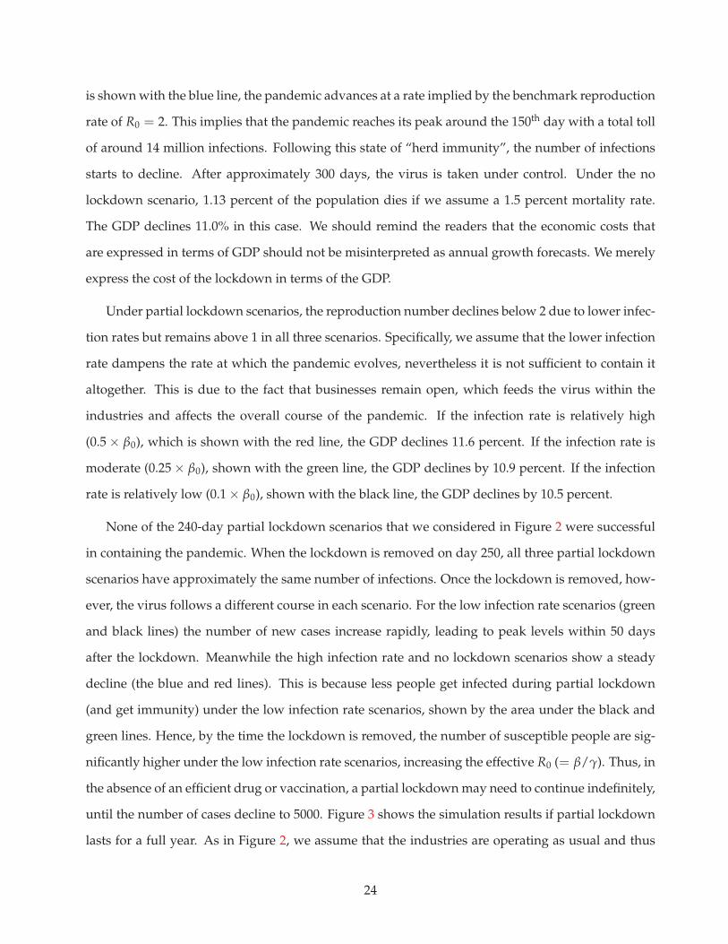
is shown with the blue line, the pandemic advances at a rate implied by the benchmark reproduction

rate of R0 = 2. This implies that the pandemic reaches its peak around the 150th day with a total toll

of around 14 million infections. Following this state of “herd immunity”, the number of infections

starts to decline. After approximately 300 days, the virus is taken under control. Under the no

lockdown scenario, 1.13 percent of the population dies if we assume a 1.5 percent mortality rate.

The GDP declines 11.0% in this case. We should remind the readers that the economic costs that

are expressed in terms of GDP should not be misinterpreted as annual growth forecasts. We merely

express the cost of the lockdown in terms of the GDP.

Under partial lockdown scenarios, the reproduction number declines below 2 due to lower infec-

tion rates but remains above 1 in all three scenarios. Specifically, we assume that the lower infection

rate dampens the rate at which the pandemic evolves, nevertheless it is not sufficient to contain it

altogether. This is due to the fact that businesses remain open, which feeds the virus within the

industries and affects the overall course of the pandemic. If the infection rate is relatively high

(0.5 × β0), which is shown with the red line, the GDP declines 11.6 percent. If the infection rate is

moderate (0.25 × β0), shown with the green line, the GDP declines by 10.9 percent. If the infection

rate is relatively low (0.1 × β0), shown with the black line, the GDP declines by 10.5 percent.

None of the 240-day partial lockdown scenarios that we considered in Figure 2 were successful

in containing the pandemic. When the lockdown is removed on day 250, all three partial lockdown

scenarios have approximately the same number of infections. Once the lockdown is removed, how-

ever, the virus follows a different course in each scenario. For the low infection rate scenarios (green

and black lines) the number of new cases increase rapidly, leading to peak levels within 50 days

after the lockdown. Meanwhile the high infection rate and no lockdown scenarios show a steady

decline (the blue and red lines). This is because less people get infected during partial lockdown

(and get immunity) under the low infection rate scenarios, shown by the area under the black and

green lines. Hence, by the time the lockdown is removed, the number of susceptible people are sig-

nificantly higher under the low infection rate scenarios, increasing the effective R0 (= β/γ). Thus, in

the absence of an efficient drug or vaccination, a partial lockdown may need to continue indefinitely,

until the number of cases decline to 5000. Figure 3 shows the simulation results if partial lockdown

lasts for a full year. As in Figure 2, we assume that the industries are operating as usual and thus

24

βi’s (for i = 1, . . . , K) remain unaffected. In terms of the economic implications, the increase in the

number of infections through a second wave due to a premature reopening prevents the economy

from a jump start. Even though the supply side remains unrestricted, demand remains supressed

due to the increase in the number of infections, dragging the economic growth. These implications

are supported by a recent study Andersen et al. (2020) that compares Denmark which had a full

lockdown, with Sweden, with partial and voluntary lockdown. Aggregate spending dropped 29

per cent in Denmark and 25 per cent in Sweden. These numbers suggest that merely opening the

economy does not imply that demand will be normalized until the outbreak is contained. Thus, a

partial lockdown policy might not yield the lowest economic costs as implied by our model.

Figure 3: Alternative Scenarios under Partial Lockdown for Full Year

0

2,000

4,000

6,000

8,000

10,000

12,000

14,000

16,000

0

2,000

4,000

6,000

8,000

10,000

12,000

14,000

16,000

25 50 75 100 125 150 175 200 225 250 275 300 325 350

No lockdo wn

Partial lo ckdown w it h 1 /2* bet a0

Partial lo ckdown w it h 1 /4* bet a0

Partial lo ckdown w it h 1 /10 *be ta0

1000 pers ons

Compared to Figure 2, we observe that the main advantage of an extended partial lockdown is

that it flattens the curve by spreading the number of infections over time and allowing for a larger

recovery rate. In terms of the economic costs, the additional economic costs of the longer partial

lockdown hover around 0.5 percent of the GDP. The added costs despite the extended duration

of the lockdown are limited. This is due to the fact that the decline in demand already reaches a

maximum level at the earlier stages of the lockdown and successive reductions in production only

reflect the decline in supply due to increased number of infections.

Figure 4 illustrates the implications of our model under full lockdown. If the lockdown is put

into practice when the number of infections is around 80,000, a fully effective procedure lowers the

25

reproduction rate to zero (R0 = 0), which is shown by the blue line, and contains the pandemic

within 39 days (the gray shaded area). The consequent decline in GDP is about 5.8 percent. If the

lockdown is not very effective and the infection continues to spread with some minimal reproduc-

tion number (R0 = 0.02), then the duration of the lockdown increases by 15 days (yellow shaded

area) to 54 days and the GDP declines by 7.6 percent.

Figure 4: Alternative Scenarios under Full Lockdown

0

10

20

30

40

50

60

70

80

90

0

10

20

30

40

50

60

70

80

90

10 20 30 40 50 60 70 80 90 100 110 120 130 140 150 160 170 180 190 200

Full lockdown s tarting from 91. day with R0=0

Full lockdown starting from 91. day with R0=0.02

1000 per sons

The costs of delaying full lockdown are shown in Figure 5. The benchmark scenario that is

illustrated in Figure 4 is shown with the blue line. If the lockdown is delayed by only one day, the

number of infections increases by more than 10,000. In the model, we assume that the number of

infections increases faster than the official statistics, which report only the tested patients. Under

these circumstances, a 39-day lockdown is no longer sufficient to control the pandemic. Thus, in

exchange for a one-day delay, the lockdown needs to be extended by two more days (the red line),

which increases the costs of the lockdown to 5.9 percent of the GDP. If there is a two-day delay (the

green line), this time the duration of the lockdown increases to 43 days and the decline in GDP is 6.2

percent. If the lockdown is delayed by one week (the black line), the decline in GDP is 7.3 percent.

After 100 days, the virus starts to spread again and hence prematurely ending the lockdown is rather

ineffective.

As we compare the economic costs under full lockdown (Figures 4 and 5) with those of partial

lockdown (Figures 2 and 3), we note that the costs of full lockdown are lower than any of partial

26

Figure 5: Costs of Delay in Implementing Full Lockdown

0

40

80

120

160

200

0

40

80

120

160

200

10 20 30 40 50 60 70 80 90 100 110 120 130 140 150 160 170 180 190 200

Full lockdown starting from 91. day unt il 130. day

Full lockdown starting from 92. day unt il 132. day

Full lockdown starting from 93. day unt il 136. dayFull lockdown starting from 98. day unt il 148. day

lockdown scenarios.

As we compare the the number of deaths under alternative scenarios, we observe that 0.001 per-

cent of the population dies under an effective full lockdown, compared to 1 percent of the population

under no lockdown and about 0.8 percent of the population under partial lockdown scenarios that

last for 250 days. If partial lockdown is extended to a full year, then the number of deaths decline to

about 0.5 percent of the population.

5.3 The Role of External Demand Shocks

The aggregate costs of COVID-19 shock that we calculated in the previous section embeds supply

and demand channels in Turkey as well as abroad. In this section, we illustrate the role of external

demand and supply in total costs. In order to better illustrate the role of international linkages for

the Turkish economy, we consider two alternative scenarios.

Assuming a parallel progression of pandemics, we arrive at Equations 21, 23 and 19 to quantify

demand change and final output implied by this change. Here, different than Equation 19, in this

section we allow for country specific demand shocks. The matrix for intermediate goods is obtained

from the direct requirements matrix and the output vector:

INT = AY. (27)

27

Each entry of the matrix INT corresponds to the usage of intermediate goods by industry i in coun-

try c from industry i′ in country c′. Combining imports of intermediate goods and final goods, we

write the total imports for country c as:

importsc = ∑c′ 6=c

n

∑i=1

(

Fc,c′,i +n

∑i′=1

INTc,i,c′,i′

)

(28)

Similarly the total exports by country c is:

exportsc = ∑c′ 6=c

n

∑i=1

(

Fc′,c,i +n

∑i′=1

INTc′,i′,c,i

)

(29)

As a result, a decline in foreign demand for final goods will create sectoral output declines in

many domestic sectors, which will add to aggregate output decline in Turkey. To highlight this

mechanism, we present three scenarios.

Scenario 1 assumes the same proportionate demand shock in Equation 19 for the whole world.

For example, if we estimate that the demand for automobiles decline by 60 percent based on Turk-

ish data, we assume that the demand for automobiles declines by 60 percent throughout the world.

Figure 6 shows how much total output, exports and imports change at the brunt of the pandemic

relative to normal times for alternative scenarios. In the baseline scenario, the decline in terms of

total output is 19.8 percent (Scenario 1 in Figure 6). Interestingly, imports decline less (17.9 percent)

compared to exports (23.4 percent). This is consistent with the nature of the Turkish economy which

is highly dependent on imports of intermediate goods. On the exports side, a further breakdown

indicates that the 27.4% decline in terms of final goods is higher than the 18.8% decline in interme-

diate goods (not shown). Similarly, on the imports side, the 19.7% decline in intermediate goods is

higher than the 16.1% decline in final goods (not shown).

Under scenario 2, we assume that the demand in Turkey declines but the international demand

for final goods is back to its normal (see Scenario 2 in Figure 6). Using the automobile example

above, this implies that the domestic demand for automobiles shrinks to 60% of normal levels but

the international demand remains at its normal levels. In this setting, the decline in terms of total

output is 14.6 percent at the brunt of the pandemic. The decline in imports is 14.7% but the decline

28

Figure 6: Demand Shocks for an Open Economy with I-O Links

-19.8

-23.4

-17.9

-14.6

-.1

-14.7

-5.2

-23.3

-3.2

-25

-20

-15

-10

-50

Scenario 1 Scenario 2 Scenario 3

Output Exports

Imports

NOTES: This graph illustrates the impact of three different scenarios for demand shocks. In the first scenario, all thecountries are assumed to experience the same demand shifter during the pandemic. In the second scenario, only Turkeyexperiences a demand shock but the international demand levels are intact. In the final scenario, the internationaldemand levels are down but the demand in Turkey is at pre-pandemic levels. The number written on each barcorresponds to the percentage change in the relevant variable in the underlying scenario relative to its pre-pandemiclevel.

in exports is only 0.1%.

Lastly, in scenario 3, we model the setting where the demand in Turkey is intact but the demand

in international markets has plummeted (see Scenario 3 in Figure 6). Under this scenario, the decline

in output is 5.2% solely because of international linkages. As expected, the exports are hit the hardest

with a decline of 23.3% and imports decline by 3.2%.

If we compare Scenario 1 and Scenario 3, we can see the role of demand in total economic costs.

The decline in foreign demand solely account for almost 27 percent of the decline in aggregate out-

put. Notice that we run these scenarios under no lockdown policy in the absence of any policy

action.

29

5.4 Globally Uncoordinated Lockdowns and the Role of Fiscal Policy

So far we assumed that the countries act in global coordination and take measures similar to Turkey

during the pandemic. In this section, we relax this assumption to calculate the economic costs in

an environment of uncoordination. The purpose of this exercise is to take a closer look at the role

of foreign demand on the domestic recovery through two channels: First, we want to determine

the additional costs that will be borne by the small open economy, if its trade partners do not take

effective lockdown measures to contain the pandemic. Second, we want to quantify the role of fiscal

stimulus that is provided by the trade partners on domestic recovery.

In order to compute these alternative scenarios, we make several simplifying assumptions. Specif-

ically, we assume that countries consider either full lockdown or partial lockdown during the pan-

demic. In a full lockdown, many industries are either fully or partially closed, hence, their supplies

are lower. We further simplify our definition of a partial lockdown. In the previous section, both

demand and supply shocks were present during a partial lockdown. In this section, we ignore the

supply effects through the labor force due to sick workers. This enables us to pinpoint solely the

foreign demand related losses in the home country due to the lack of global coordination. Further-

more, this simplification is strengthened by our findings in the next section where we find that the

demand shock is more assertive than the supply shock during a partial lockdown (Figure 9, panel c).

When the lockdowns are not coordinated, we assume that the countries in the rest of the world

choose between a full lockdown and a partial lockdown when the home country (i.e. Turkey) imple-

ments full lockdown. In this manner, we calculate the additional costs that Turkey would bear due

to the decline in external demand, depending on the number of infections in its trade partners.

To allow for different lockdown decisions and hence differential progression of the pandemic

in countries, we ignore the sectoral heterogeneity and assume a single β for a country. Lockdown

decisions affect this β value. Full lockdowns bring β = 0 and partial lockdown bring it down to half

the value, i.e., β = 0.14/2.

In this section, we assume that the countries start the pandemic with the same number of infec-

tions. Once the infection levels reach Ic = populationc/1000 for country c, it goes into lockdown.

With these simplifying assumptions, the decision of an initial lockdown coincides across countries.

30

Table 1: ECONOMIC COSTS OF THE PANDEMIC UNDER DIFFERENT GLOBAL SCENARIOS

Scenario: Coordinated FL (ρ=1) Uncoordinated FL (ρ=0.5) Uncoordinated FL (ρ=0)

(1) (2) (3)

(1) Without stimulus 5.8 6.9 7.8(2) With stimulus 6.6 7.4

NOTES: Table 1 reports the economic costs of the pandemic under different scenarios. Coordinated FL (ρ=1): A lockdownis put into practice between the 91st and 131st days of the pandemic and is fully effective with zero reproduction numberin Turkey and the rest of the world coordinates with Turkey i.e., the probability of coordination (ρ) equals 1;Uncoordinated FL (ρ=0.5): A lockdown is put into practice in between the 91st and 131st days of the pandemic and isfully effective with zero reproduction number within Turkey and a randomly selected 50 percent of the countries in theworld cooperate with Turkey i.e., ρ=0.5; Uncoordinated FL (ρ=0): A lockdown is put into practice in between the 91st and131st days of the pandemic and is fully effective with zero reproduction number within Turkey, but the rest of the worlddoes not cooperate with Turkey i.e., ρ=0. The economic costs are computed also for additional scenarios where thecountries that implement partial lockdown consider stimulus packages or not.

However, further lockdown decisions can take place at different times since some countries choose

partial lockdown while others engage in full lockdown and follow different paths. We model several

scenarios that are summarized in Table 1.

In our baseline scenario, all countries go into full lockdown simultaneously and the disease is

controlled globally after 39 days. The results from this scenario were reported in the previous sec-

tion 5.2 where the total costs were estimated to be 5.8 percent. We replicate this figure in Table 1

for comparison purposes (column 1). In the two alternative scenarios, we allow for uncoordination

and let a certain fraction of the countries adopt partial lockdown while Turkey still maintains a full

lockdown. The additional cost incurred by Turkey, compared to our baseline scenario reflects the

impact of foreign demand on Turkey’s pandemic-related costs.

In the second scenario, we assume that Turkey goes into full lockdown and all other countries are

assigned to full or partial lockdown with equal probability (Table 1, column 2). We run this scenario

200 times to control for the effect of random assignment and to establish confidence intervals. We

note that the economic costs borne by Turkey increase to 6.9 percent when some of its trade partners

suffer from a prolonged pandemic and reduce their demand for Turkish goods. In the third scenario,

we provide an upper bound for the additional costs that are accrued due to lower external demand.

This time, we assume that Turkey goes into full lockdown and all other countries engage in partial

lockdown. This scenario yields the highest costs of 7.9 percent (Table 1, column 3).

31

Next, we consider a framework where the countries that implement partial lockdown consider

stimulus packages to offset the sizable reduction in demand in their economies. In our set up, this

corresponds to increasing η by 5 percent in Equation 16. With this interpretation, the stimulus pack-

ages enable the consumers to increase their budget for the expenditures and lead to a milder decline

in the demand profile. In other words, we assume that the fiscal stimulus that is given to the con-

sumers result in a 5% increase (i.e. 1.05 × η) in spending at any point of the pandemic.

Let us again remind the readers that the next section compares the relative importance of supply

and demand factors under alternative lockdown scenarios. In that section we illustrate that the

demand effect is dominant in a partial lockdown, which drags economic costs (Figure 9, panel c).

Thus, policies that are aimed to stimulate demand are most effective in a partial lockdown.18 In

light of this finding, we consider stimulus programs only under partial lockdown. The second row

in Table 1 illustrates that total economic costs in the home country decline by about 0.3 to 0.4 percent

of the GDP if the countries that adopt partial lockdowns offset some of the drag in their economies

through stimulus packages.

We note that the costs of uncoordinated lockdown that we estimated in this section do not incor-

porate the potential future waves once the home country considers an effective full lockdown and

reduces the number of infections to 5000. In our stylized model, we assume that the home coun-

try can implement effective contact tracing and keep the pandemic contained moving forward. In

real life, an uncoordinated lockdown in the absence of vaccinations magnifies global and domestic

economic costs by causing the virus to circulate and present potential risks for the home country.

In terms of the fiscal policy implementation, the stimulus package announced by the Turkish

government in March 2020 was consistent with the general framework adopted by other countries.

There was postponement of tax obligations, social security premiums and credit payments of the

companies in the services sector. The limits of the Credit Guarantee Fund were increased to make

bank loans more accessible. Temporary income support was provided to those workers whose com-

panies have ceased production due to the pandemic. Furthermore, a cash assistance program for

needy families was launched. IMF data notes that once equity, loans, and guarantees are excluded,

18In contrast, supply side pressures characterize total costs in a full lockdown. Therefore, we do not consider demand-side policies if the countries adopt full lockdown

32

fiscal spending in Turkey was less than 2 percent in 2020, the third lowest among EMs after Mexico

and Egypt. This reflects the limited fiscal space relative to other EMs and advanced economies.19

5.5 Sectoral Breakdown of Economic Costs

In this section, we analyze the economic costs at the sectoral level. Heterogeneity in sectoral costs

may stem from several channels. Sectors that are closed down due to isolation measures (i.e. nonessen-

tial sectors), those that are hit hardest by the collapse in demand such as the services sectors, or

those industries where teleworking is not very feasible will be hit harder. As for the role of inter-

national linkages, those sectors with greater exposure to international spillovers, particularly with

those countries that had larger domestic outbreaks would be more affected. Similarly, those indus-

tries that rely more on external finance would experience the pinch of tightening in global financial

conditions. In the next sub-section, we focus on the role of trade linkages. In the following sub-

section, we calculate the sectoral economic costs in our framework under different scenarios. Using

these sectoral costs, in the last sub-section, we disentangle the role of trade and external funding in

sectoral costs in a regression framework.

5.5.1 The Role of Trade Linkages in Sectoral Costs

We investigate the role of international linkages in determining the heterogenetiy in sectoral costs.

International linkages would affect economic costs through trade relationships as well as capital

inflows, both at the sectoral level. Those sectors that are more closely connected to international

value chains as well as those sectors that are dependent on external funding would be affected more

from the COVID-19 shock.

Figure 7 allows us to get a glimpse of the role of trade. The figure illustrates the share of im-

ports in total intermediate inputs (the left panel) and the share of exports in total output (the right

panel). We would expect those sectors that rely on imports and exports to be more affected. For

example, motor vehicles, transportation equipment, electrical equipment, computer and electronics,

and tourism-related services sectors such as accommodation and food services are the sectors that

19https://www.imf.org/en/Topics/imf-and-covid19/Fiscal-Policies-Database-in-Response-to-COVID-19.

33

rely more on external demand. Thus, the deep recessions that are expected in Turkey’s major export

markets such as the Euro Area, UK, or the US would hit these sectors the most, consistent with our

analysis in Figure 6.

Figure 7: Import and Export Share

(a) Import Share in Intermediate Inputs

010

20

30

40

Share

of Im

port

s in Inte

rmedia

te Inputs

Agricultu

re &

Fishing

Mining

(Ene

rgy)

Mining

(Non

-Ene

rgy)

Mining

Suppo

rt

Food,

Bev

. & Tob

.

Textile

s & A

ppar

el

Woo

d Pro

d.

Paper

Pro

d.

Cok

e & R

ef P

etro

l.

Che

m. &

Pha

rma

Rub

ber &

Plastic

Oth

er N

on-M

etal

Basic M

etals

Fabric

ated

Met

al

Com

p., E

lectr.

& Opt

.

Electric

al E

q.

Mac

hine

ry &

Eq.

, NEC

Mot

or V

ehicles

Oth

er T

rans

port

Eq.

Oth

er M

anuf

actu

ring

Public

Wor

ks

Con

stru

ction

Who

lesa

le &

Ret

ail

Tran

spor

t. & S

tora

ge

Accom

. & F

ood

Serv.

Publis

h. &

Bro

adca

st.

Teleco

mm

unicat

ions

IT &

Oth

er In

f.

Finan

ce &

Insu

ranc

e

Rea

l Estat

e

Oth

er B

usines

s Ser

v.

Public

Adm

in. &

Def

.

Educa

tion

Hea

lth &

Soc

ial W

ork

Arts, E

nt. &

Rec

.

(b) Export Share in the Output

010

20

30

40

50

Share

of E

xport

s in T

ota

l O

utp

ut

Agricultu

re &

Fishing

Mining

(Ene

rgy)

Mining

(Non

-Ene

rgy)

Mining

Suppo

rt

Food,

Bev

. & Tob

.

Textile

s & A

ppar

el

Woo

d Pro

d.

Paper

Pro

d.

Cok

e & R

ef P

etro

l.

Che

m. &

Pha

rma

Rub

ber &

Plastic

Oth

er N

on-M

etal

Basic M

etals

Fabric

ated

Met

al

Com

p., E

lectr.

& Opt

.

Electric

al E

q.

Mac

hine

ry &

Eq.

, NEC

Mot

or V

ehicles

Oth

er T

rans

port

Eq.

Oth

er M

anuf

actu

ring

Public

Wor

ks

Con

stru

ction

Who

lesa

le &

Ret

ail

Tran

spor

t. & S

tora

ge

Accom

. & F

ood

Serv.

Publis

h. &

Bro

adca

st.

Teleco

mm

unicat

ions

IT &

Oth

er In

f.

Finan

ce &

Insu

ranc

e

Rea

l Estat

e

Oth

er B

usines

s Ser

v.

Public

Adm

in. &

Def

.

Educa

tion

Hea

lth &

Soc

ial W

ork

Arts, E

nt. &

Rec

.

NOTES: (a) This figure plots the share of imports in the intermediate inputs. (b) This figure plots the exports as a share ofoutput for each sector. Source: OECD ICIO Tables.

5.5.2 The Role of Lockdowns on Sectoral Costs

Figure 8 shows how hard each sector is hit from the pandemic under alternative lockdown scenarios.

Consistent with our earlier findings, we observe that the full lockdown has the lowest economic

costs compared to the alternatives. In terms of sectoral heterogeneity, we note that teleworkable

or essential sectors are less severely affected because they continue functioning for all lockdown

scenarios (such as education, IT, public administration). Meanwhile, non-essential sectors or those

that require on-site work are more severely affected (such as accommodation and food services, arts,

entertainment, and recreation, construction).

After documenting the heterogeneous economic costs of the pandemic for different sectors, we

investigate whether these costs are accrued from demand or supply pressures. Figure 9 counts the

days in which output implied by the demand channel or supply channel prevails to bring about the

equilibrium output in a given industry.

34

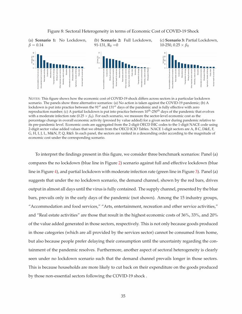
Figure 8: Sectoral Heterogeneity in terms of Economic Cost of COVID-19 Shock

(a) Scenario 1: No Lockdown,β = 0.14

010

20

30

40

VA

loss (

%)

Accom

modation &

food s

erv

ices

Art

s,e

nte

rtain

ment &

recre

ation

Real esta

te a

ctivitie

s

Constr

uction

Manufa

ctu

ring

Tra

nsport

ation &

sto

rage

Min

ing &

quarr

yin

g

Oth

er

busin

ess s

ecto

r serv

ices

Ele

ctr

icity, w

ate

r &

waste

Education

Info

rmation &

com

munic

ation

Whole

sale

& R

eta

il

Agriculture

, fo

restr

y &

fis

hin

g

Public

Adm

.

Hum

an h

ealth &

socia

l w

ork

(b) Scenario 2: Full Lockdown,91-131, R0 =0

05

10

15

VA

loss (

%)

Accom

modation &

food s

erv

ices

Constr

uction

Min

ing &

quarr

yin

g

Art

s,e

nte

rtain

ment &

recre

ation

Hum

an h

ealth &

socia

l w

ork

Manufa

ctu

ring

Real esta

te a

ctivitie

s

Oth

er

busin

ess s

ecto

r serv

ices

Agriculture

, fo

restr

y &

fis

hin

g

Public

Adm

.

Education

Tra

nsport

ation &

sto

rage

Info

rmation &

com

munic

ation

Ele

ctr

icity, w

ate

r &

waste

Whole

sale

& R

eta

il

(c) Scenario 3: Partial Lockdown,10-250, 0.25 × β0

010

20

30

40

VA

loss (

%)

Accom

modation &

food s

erv

ices

Art

s,e

nte

rtain

ment &

recre

ation

Real esta

te a

ctivitie

s

Constr

uction

Manufa

ctu

ring

Tra

nsport

ation &

sto

rage

Min

ing &

quarr

yin

g

Oth

er

busin

ess s

ecto

r serv

ices

Ele

ctr

icity, w

ate

r &

waste

Education

Info

rmation &

com

munic

ation

Whole

sale

& R

eta

il

Agriculture

, fo

restr

y &

fis

hin

g

Public

Adm

.

Hum

an h

ealth &

socia

l w

ork

NOTES: This figure shows how the economic cost of COVID-19 shock differs across sectors in a particular lockdownscenario. The panels show three alternative scenarios: (a) No action is taken against the COVID-19 pandemic; (b) Alockdown is put into practice between the 91st and 131st days of the pandemic and is fully effective with zeroreproduction number; (c) A partial lockdown is put into practice between 10th-250th days of the pandemic that evolveswith a moderate infection rate (0.25 × β0). For each scenario, we measure the sector-level economic cost as thepercentage change in overall economic activity (proxied by value added) for a given sector during pandemic relative toits pre-pandemic level. Economic costs are aggregated from the 2-digit OECD ISIC codes to the 1-digit NACE code using2-digit sector value added values that we obtain from the OECD ICIO Tables. NACE 1-digit sectors are A, B C, D&E, F,G, H, I, J, L, M&N, P, Q, R&S. In each panel, the sectors are ranked in a descending order according to the magnitude ofeconomic cost under the corresponding scenario.

To interpret the findings present in this figure, we consider three benchmark scenarios: Panel (a)

compares the no lockdown (blue line in Figure 2) scenario against full and effective lockdown (blue

line in Figure 4), and partial lockdown with moderate infection rate (green line in Figure 3). Panel (a)

suggests that under the no lockdown scenario, the demand channel, shown by the red bars, drives

output in almost all days until the virus is fully contained. The supply channel, presented by the blue

bars, prevails only in the early days of the pandemic (not shown). Among the 15 industry groups,

“Accommodation and food services,” “Arts, entertainment, recreation and other service activities,”

and “Real estate activities” are those that result in the highest economic costs of 36%, 33%, and 20%

of the value added generated in those sectors, respectively. This is not only because goods produced

in those categories (which are all provided by the services sector) cannot be consumed from home,

but also because people prefer delaying their consumption until the uncertainty regarding the con-

tainment of the pandemic resolves. Furthermore, another aspect of sectoral heterogeneity is clearly

seen under no lockdown scenario such that the demand channel prevails longer in those sectors.

This is because households are more likely to cut back on their expenditure on the goods produced

by those non-essential sectors following the COVID-19 shock .

35

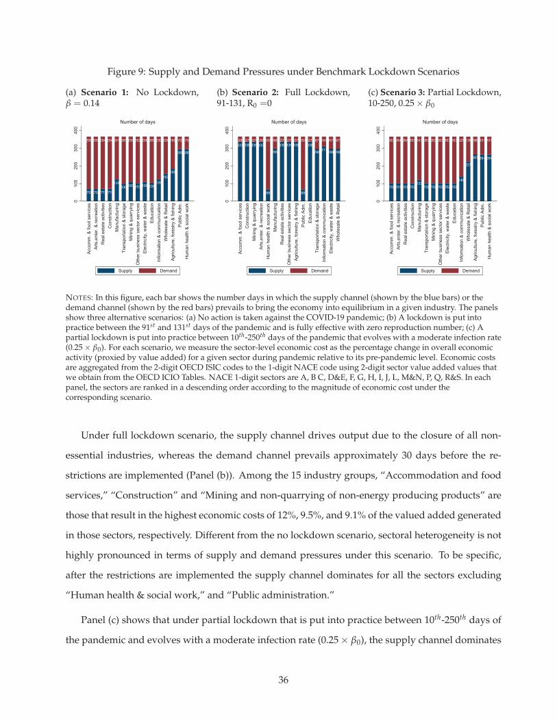
Figure 9: Supply and Demand Pressures under Benchmark Lockdown Scenarios

(a) Scenario 1: No Lockdown,β = 0.14

70

295

70

295

71

294

71

294

124

241

100

265

109

256

103

262

109

256

105

260

126

239

157

208

185

180

295

70

295

70

01

00

20

03

00

40

0

Acco

mm

. &

fo

od

se

rvic

es

Art

s,e

nte

r. &

re

cre

atio

n

Re

al e

sta

te a

ctivitie

s

Co

nstr

uctio

n

Ma

nu

factu

rin

g

Tra

nsp

ort

atio

n &

sto

rag

e

Min

ing

& q

ua

rryin

g

Oth

er

bu

sin

ess s

ecto

r se

rvic

es

Ele

ctr

icity, w

ate

r &

wa

ste

Ed

uca

tio

n

Info

rma

tio

n &

co

mm

un

ica

tio

n

Wh

ole

sa

le &

Re

tail

Ag

ricu

ltu

re, fo

restr

y &

fis

hin

g

Pu

blic

Ad

m.

Hu

ma

n h

ea

lth

& s

ocia

l w

ork

Number of days

Supply Demand

(b) Scenario 2: Full Lockdown,91-131, R0 =0

337

28

338

27

338

27

337

28

68

297

299

66

338

27

338

27

338

27

68

297

338

27

298

67

311

54

298

67

298

67

01

00

20

03

00

40

0

Acco

mm

. &

fo

od

se

rvic

es

Co

nstr

uctio

n

Min

ing

& q

ua

rryin

g

Art

s,e

nte

r. &

re

cre

atio

n

Hu

ma

n h

ea

lth

& s

ocia

l w

ork

Ma

nu

factu

rin

g

Re

al e

sta

te a

ctivitie

s

Oth

er

bu

sin

ess s

ecto

r se

rvic

es

Ag

ricu

ltu

re, fo

restr

y &

fis

hin

g

Pu

blic

Ad

m.

Ed

uca

tio

n

Tra

nsp

ort

atio

n &

sto

rag

e

Info

rma

tio

n &

co

mm

un

ica

tio

n

Ele

ctr

icity, w

ate

r &

wa

ste

Wh

ole

sa

le &

Re

tail

Number of days

Supply Demand

(c) Scenario 3: Partial Lockdown,10-250, 0.25 × β0

102

263

101

264

101

264

102

263

122

243

102

263

102

263

102

263

102

263

102

263

140

225

227

138

267

98

264

101

264

101

01

00

20

03

00

40

0

Acco

mm

. &

fo

od

se

rvic

es

Art

s,e

nte

r. &

re

cre

atio

n

Re

al e

sta

te a

ctivitie

s

Co

nstr

uctio

n

Ma

nu

factu

rin

g

Tra

nsp

ort

atio

n &

sto

rag

e

Min

ing

& q

ua

rryin

g

Oth

er

bu

sin

ess s

ecto

r se

rvic

es

Ele

ctr

icity, w

ate

r &

wa

ste

Ed

uca

tio

n

Info

rma

tio

n &

co

mm

un

ica

tio

n

Wh

ole

sa

le &

Re

tail

Ag

ricu

ltu

re, fo

restr

y &

fis

hin

g

Pu

blic

Ad

m.

Hu

ma

n h

ea

lth

& s

ocia

l w

ork

Number of days

Supply Demand

NOTES: In this figure, each bar shows the number days in which the supply channel (shown by the blue bars) or thedemand channel (shown by the red bars) prevails to bring the economy into equilibrium in a given industry. The panelsshow three alternative scenarios: (a) No action is taken against the COVID-19 pandemic; (b) A lockdown is put intopractice between the 91st and 131st days of the pandemic and is fully effective with zero reproduction number; (c) Apartial lockdown is put into practice between 10th-250th days of the pandemic that evolves with a moderate infection rate(0.25 × β0). For each scenario, we measure the sector-level economic cost as the percentage change in overall economicactivity (proxied by value added) for a given sector during pandemic relative to its pre-pandemic level. Economic costsare aggregated from the 2-digit OECD ISIC codes to the 1-digit NACE code using 2-digit sector value added values thatwe obtain from the OECD ICIO Tables. NACE 1-digit sectors are A, B C, D&E, F, G, H, I, J, L, M&N, P, Q, R&S. In eachpanel, the sectors are ranked in a descending order according to the magnitude of economic cost under thecorresponding scenario.

Under full lockdown scenario, the supply channel drives output due to the closure of all non-

essential industries, whereas the demand channel prevails approximately 30 days before the re-

strictions are implemented (Panel (b)). Among the 15 industry groups, “Accommodation and food

services,” “Construction” and “Mining and non-quarrying of non-energy producing products” are

those that result in the highest economic costs of 12%, 9.5%, and 9.1% of the valued added generated

in those sectors, respectively. Different from the no lockdown scenario, sectoral heterogeneity is not

highly pronounced in terms of supply and demand pressures under this scenario. To be specific,

after the restrictions are implemented the supply channel dominates for all the sectors excluding

“Human health & social work,” and “Public administration.”

Panel (c) shows that under partial lockdown that is put into practice between 10th-250th days of

the pandemic and evolves with a moderate infection rate (0.25 × β0), the supply channel dominates

36

in the first 100 days of pandemic. On the other hand, demand drives output for the rest of the year,

including the days in which new peak levels are reached after the partial lockdown is prematurely

removed. This is because of the fact that businesses remain open, which feeds the virus within the

industries and increases the uncertainty about the containment of the pandemic. Among the 15

industry groups, “Accommodation and food services,” “Arts, entertainment, recreation and other

service activities,” and “Real estate activities” are those that result in highest economic costs of 36%,

34%, and 21% of the value added generated in those sectors, respectively. We note that sectoral

heterogeneity in terms of supply and demand pressures is very similar to the no lockdown scenario.

5.5.3 The Role of External Finance in Sectoral Costs

If the sectors that have closer trade linkages to the rest of the world suffer more from uncoordinated

lockdowns, then a natural question is whether external finance can help the fiscal needs of these

sectors.

To investigate this question, we consider a regression specification at the sector-level. Specifically,

we regress the economic cost in each sector onto sectoral trade and sectoral capital flows under

different lockdown scenarios to highlight the role of external linkages in driving these costs. Recall

from panel (a) in Figure 9 that in the case of a global no lockdown, demand channel drives output,

leading to demand-driven economic costs of the pandemic. In contrast, panel (b) illustrates that

supply channel is dominant in the case of a globally coordinated full lockdown, reducing the role

of external as well as domestic demand. Consequently, in the regression results below, we expect

to find the role of external linkages to increase as the lockdown measures become less strict in the

trade partners of home country in an environment of uncoordinated lockdowns.

We use data from international I-O matrix to measure sectoral trade. For sectoral capital flows,

we use a sectoral weighted average of country-pair capital flows, where sector shares come from

37

Table 2: SECTOR-LEVEL REGRESSIONS

Scenario: No Lockdown Uncoordinated FL (ρ=0) Uncoordinated FL (ρ=0.5) Coordinated FL (ρ=1)

(1) (2) (3) (4) (5) (6) (7) (8) (9) (10) (11) (12)

Dep. Var: VA Loss

(1) Trade 16.0273** 16.5283** 6.1316* 6.5342** 5.5668* 5.9434** 4.5942* 4.9384** 4.2206* 4.5493** 1.1996 1.4767(6.388) (6.412) (3.039) (2.925) (2.876) (2.772) (2.340) (2.223) (2.243) (2.132) (1.919) (1.847)

(2) Capital Flows 34.9502* 35.8033** 15.9595 16.6450* 14.0993 14.7406* 12.2088* 12.7950* 11.0549 11.6147* 4.8717 5.3435(17.331) (17.234) (9.638) (9.201) (8.973) (8.571) (6.979) (6.558) (6.623) (6.222) (5.274) (4.988)

(3) FX 0.1572** 0.1263** 0.1182** 0.1080** 0.1031** 0.0869**(0.076) (0.041) (0.039) (0.032) (0.031) (0.034)

Stimulus package No No No No Yes Yes No No Yes Yes No No

R2 0.12 0.2 0.041 0.19 0.039 0.19 0.032 0.19 0.03 0.18 0.0036 0.11

NOTES: Table 2 reports the results of estimation of Equation 30 for four alternative scenarios. No Lockdown: No action istaken against the COVID-19 pandemic; Coordinated FL (ρ=1): A lockdown is put into practice between the 91st and 131st

days of the pandemic and is fully effective with zero reproduction number in Turkey and the rest of the world coordinatewith Turkey i.e., the probability of coordination (ρ) equals 1; Uncoordinated FL (ρ=0.5): A lockdown is put into practicein between the 91st and 131st days of the pandemic and is fully effective with zero reproduction number within Turkeyand a randomly selected 50 percent of the countries in the world cooperate with Turkey i.e., ρ=0.5; Uncoordinated FL(ρ=0): A lockdown is put into practice in between the 91st and 131st days of the pandemic and is fully effective with zeroreproduction number within Turkey, but the rest of the world do not cooperate with Turkey i.e., ρ=0. We report theresults for additional scenarios where the countries that implement partial lockdowns consider stimulus packages or not.Dependent variable is defined as sector-level economic cost of the COVID-19 shock that is measured as the percentagechange in overall economic activity proxied by value added for a given sector during pandemic relative to itspre-pandemic level. Heteroskedastic-consistent standard errors are reported in parentheses. ***, **, and * indicatesignificance at the 1%, 5%, and 10% levels, respectively.

sectoral trade.20,21 And then we run the following regression for sector i:

∆Yi = β0 + β1Tradei + β2Capital Flowsi + ε i (30)

where ∆Yi stands for the economic cost of the COVID-19 shock for sector i for i = 1, . . . , K, that

we estimate under different lockdown scenarios. We measure the sector-level economic cost as the

percentage change in overall economic activity (proxied by value added (VAi), where value added

equals total production minus intermediate inputs i.e., VAi=Yi-INTi.) for a given sector during pan-

demic relative to its pre-pandemic level.

The regression results are highly consistent with our expectations. The positive and highly signif-

20We calculate the sector-level proxy as follows: Capital Flowsi =n

∑c=1

(((Exportsc,i − Importsc,i)/Outputi) ×

Capital Flowsc)/n where Exportsc,i, Importsc,i and Outputi refer to final goods and intermediate goods made in sectori to be sold in the corresponding country c, final goods and intermediate goods that are bought from the correspondingcountry c to be used in sector i, and total output produced in sector i, respectively.

21The related data on capital flows is obtained from BIS and it is publicly available at https://stats.bis.org/statx/srs/table/A6.2?c=TR&p=20194&m=. Capital flows data of Turkey from 26 countries refers to data on Turkish banking sectorexternal liabilities vis-a-vis those countries for 2019-Q4. We normalize flows by GDP as of 2019.

38

icant coefficient estimates in the first two columns of Table 2 confirm the importance of international

linkages on sectoral COVID losses under no lockdown scenario. The results suggest that sectors

with stronger trade links suffer from larger COVID-19 related losses due to a significant decline

in external demand (row 1). They further suggest that sectors who finance these stronger produc-

tion links through capital flows (row 2) and sectors with higher FX exposure (row 3) suffer even

more, highlighting the additional adverse impact of COVID-19 on EMs with high external debt and

domestic FX debt. We control sectoral FX debt (measured as the ratio of foreign currency debt in

total debt as of 2016) because this variable captures domestic sectoral borrowing in foreign currency

as opposed to international borrowing that we want to capture and hence will create an omitted

variable bias.

Columns (3) to (12) illustrate the regression results where we use the sectoral COVID losses

that are estimated under uncoordinated and coordinated full lockdown scenarios. In an uncoor-

dinated lockdown where the rest of the world adopts partial lockdown while Turkey implements

full lockdown (columns (3) to (6)), there is still a significant positive relationship between the sec-

toral costs and trade linkages, stemming from the decline in demand for Turkish exports despite the

containment of the pandemic in Turkey. Columns (3) and (4) illustrate that the coefficient estimates

associated with trade linkages decline more than 50 percent compared to the no-lockdown scenario

thanks to the improvement in external demand due to lockdown measures abroad. The coefficient

estimates decline further if the countries that implement partial lockdown provide stimulus pack-

ages (columns (5) and (6)) to support their recovery. The consequent improvement in the export

revenue reduce the pandemic related costs at the home country.

If half of the world adopts full lockdown together with Turkey (columns (7) to (10)), then the em-

pirical relationship weakens further because foreign demand strengthens as more countries adopt

stricter lockdown measures. Within this scenario, adoption of fiscal stimulus programs further

weaken the relationship as shown in columns (9) and (10). If the lockdown is completely coordi-

nated and all countries adopt full lockdown (columns (11) and (12)), this time external demand fully

normalizes. Indeed, in this scenario, the significant relation between sectoral output losses and trade

and finance linkages disappears as the export revenue rebounds quickly following the containment

of pandemic in all trade partners of Turkey. Put differently, now there is almost no sectoral variation

39

on the left hand side that can be linked to open economy linkages. The coefficient on FX debt re-

mains positive and significant with a similar magnitude. This debt is mostly borrowed domestically

and hence still linked to the sectoral variation in COVID losses. Specifically, sectors with higher FX

debt will suffer from COVID related deprecation, incurring higher COVID losses.

5.6 Comparing the Model’s Predictions to Real-Life Experiences

When we take a look at the experiences of the countries over the course of the pandemic, we note

that there are several paths adopted by different countries:

(i) Full lockdown: China, New Zealand, and Denmark provide good examples for an effective

full lockdown. Our analysis indicates that this is the policy that minimizes economic costs by

containing the pandemic in the most effective way.

(ii) No lockdown: Very few countries considered no lockdown since the beginning of the pan-

demic. No lockdown approach might yield lower economic costs but the death toll is signifi-

cantly higher. The economic costs are mostly dependent on the changes in demand.

(iii) Partial lockdown followed by full lockdown: Many countries followed this route including

Italy, France, Germany, Spain, Iran, Russia among others. Several of these counties recently

announced that they will gradually lift restrictions. The duration of full lockdown is longer

than it could have been, had it been implemented earlier. In Italy, for example, a full lockdown

went into effect on March 10, and the restrictions are announced to be removed by May 4, after

approximately two months under full lockdown.

(iv) Enhanced Partial lockdown: Turkey started with immediate partial lockdown measures which

were enhanced over the course of the pandemic. Schools were closed on March 16 and the

businesses were encouraged to work remotely where possible. On March 21, a curfew was

imposed for people above the age of 65 and those with chronic diseases. The curfew was

extended to those younger than 20 on April 5, effectively putting close to 40% of the popula-

tion under full lockdown. Furthermore, a full lockdown was implemented on weekends and

national holidays starting on April 9 in 31 largest cities which constitute approximately 87%

40

of the population.22 After about 45 days since the beginning of enhanced partial lockdown

measures, R0 is reduced below 1 and the number of new patients is lower than the number of

recovered patients as of the last week of April.

(v) Full or Partial lockdown followed by pre-mature openings As the pandemic extended into

its second year, many countries loosened the lockdown restrictions prematurely and had to re-

introduce them as the number of infections increased, generating second and the third waves

consistent with our analysis of pre-mature openings.

Figure 10 illustrates the course of the pandemic for a selected group of countries including Italy,

New Zealand, the United Kingdom, the United States, and Turkey. Except for New Zealand, most of

the other countries opened up their economies prematurely and experienced multiple waves. New

Zealand, on the other hand, was able to implement an effective full lockdown early on and contained

the outbreak afterwards. This figure matches very well with the figures from our model in terms of

the effects of different lockdowns. New Zealand mimics our illustration of an effective lockdown in

Figure 10 while the rest of the countries mimic partial lockdown with premature opening scenario

illustrated in Figure 2.

Where does this take us? Our analysis indicates that a full lockdown at the early stages of

the crisis can bring the pandemic under control relatively quickly. There are countries who im-

plemented this successfully but also countries such as India, who tried an early full lockdown but

did not succeed. The individual performance of the country depends on several factors that affect

the recovery and the infection rates. An evaluation of Turkey’s performance, one year after the in-

troduction of lockdown measures indicates that Turkey did reasonably well during the first wave.

Potential reasons for the superior performance are the remarkable ICU capacity, young population,

less care homes, as well as the generally compliant population where government decrees are not

challenged.23As the pandemic extended, however, Turkey was among many other countries that

removed the restrictions too soon and faced consequential waves in the number of infections. As

the duration of lockdown increases, policy makers get anxious about opening up their economies.

22These cities include the 30 metropolitan municipalities and Zonguldak, which constitute close to 79% of the pop-ulation. On top of these, the age-based restrictions are intact in the rest of Turkey, which increases the number close to87%.

23See https://blogs.lse.ac.uk/covid19/2020/06/04/how-has-turkey-done-in-its-fight-against-covid-19-the-jury-is-still-out/ for a detailed evaluation of Turkey’s performance based on our framework

41

In this paper, we modelled demand as a function of the number of infections and combined this

with actual spending decline during COVID-19, measured in the data with credit card purchases.

Thus, our framework implies that demand would not normalize by the mere attempt of removing

the restrictions, so long as the number of infections are sizable. What is worse is that the number of

infections would increase again as businesses open.

In the model, we did not explicitly incorporate expectations about infections and implicitly as-

sumed that the two are highly correlated. Meanwhile, one can imagine a forward looking demand

curve, which could be a function of infection expectations rather than the actual number of infec-

tions. In this case, leaders might be able to affect expectations about the number of infections and

revive demand by removing the restrictions. To the extent that leaders can successfully convey a

more optimistic outlook, the negative demand effect that we model in this paper may weaken and

the economic costs of prematurely ending a lockdown might decline.

Another imminent issue is the potential follow up waves once the restrictions are removed. This

is particularly a problem for those countries that adopted a full lockdown at the early stages of the

crisis and controlled the pandemic in their own countries. If they open their borders, there is the

risk of a second wave. If they do not open their borders, then they cannot fully normalize and suffer

from an extended partial lockdown given the importance of the amplification effects on economic

costs for open economies. The takeaway at this stage is that if a second wave of the COVID-19 virus

hits, then an immediate and potentially global lockdown would work in the most effective way.

Our theoretical predictions are highly accurate for the Turkish economy where a relatively suc-

cessful first wave was followed by an early opening and thus a sizable second and third waves. The

consequent slowdown in demand was offset with an unsustainable credit growth policy through

low interest rates, which led to further vulnerabilities for the economy.

42

Figure 10: The Progression of COVID-19 Pandemic

(a) Italy

0

100,000

200,000

300,000

400,000

500,000

0

100,000

200,000

300,000

400,000

500,000

Feb

Mar

Apr

May Ju

n Jul

Aug

Sep

Oct

Nov D

ec Jan

Feb

Mar

20 21

(b) New Zealand

0

100

200

300

400

500

600

700

0

100

200

300

400

500

600

700

Feb

Mar

Apr

May Ju

n Jul

Aug

Sep

Oct

Nov D

ec Jan

Feb

Mar

20 21

(c) The United Kingdom

0

100,000

200,000

300,000

400,000

500,000

600,000

700,000

0

100,000

200,000

300,000

400,000

500,000

600,000

700,000

Feb

Mar

Apr

May Ju

n Jul

Aug

Sep

Oct

Nov D

ec Jan

Feb

Mar

20 21

(d) The United States

0

400,000

800,000

1,200,000

1,600,000

2,000,000

2,400,000

2,800,000

3,200,000

0

400,000

800,000

1,200,000

1,600,000

2,000,000

2,400,000

2,800,000

3,200,000

Feb

Mar

Apr

May Ju

n Jul

Aug

Sep

Oct

Nov D

ec Jan

Feb

Mar

20 21

(e) Turkey

0

50

100

150

200

250

300

0

50

100

150

200

250

300

Feb

Mar

Apr

May Ju

n Jul

Aug

Sep

Oct

Nov D

ec Jan

Feb

Mar

20 21

NOTES: Panels (a)-(d) plot the number of daily active cases in Italy, New Zealand, the United Kingdom and the UnitedStates, respectively. Panel (e) plots the number of daily deaths in Turkey.

A quickly implemented stimulus package that compensates the income loss due to the lockdown

and enables a faster recovery would minimize the long term damage in the production capacity. If

the stimulus packages are delayed, on the other hand, more companies would fail, more workers

would be laid-off, and demand would decline further. This would then feed into more bankruptcies

43

and elevate the economic costs that quickly become unmanageable. In fact, just as a drowning

person needs immediate help or else her organs start to fail, the economy needs immediate help

before the companies start to fail. Fiscal transfers can help to ensure that the supply chains are not

destroyed, the economic units are functional and ready to go back to production once the pandemic

is contained and demand returns. Fortunately, many governments around the world took decisive

action. In the case of EMs, however, policy options were limited given the limited fiscal space.

As put by former Colombian finance minister, Mauricio Cardenas: “We do not live in whatever

it takes region, we can do whatever we can.”24 The generous fiscal packages that were released

by Turkey’s trade partners supported the positive growth rate registered by the Turkish economy

in 2020 and formed expectations of export driven growth for the Turkish economy in the years

that follow. However, as noted in IMF’s country report for Turkey as of June 2021, potential GDP

in Turkey is expected to decline in the post-pandemic era, likely reflecting limited domestic fiscal

expansion during the pandemic that was unable to offset permanent damage.25

6 Conclusion

Containing the pandemic as soon as possible is an urgent obligation to save human lives. While

the introduction of vaccines is a game changer, there is still substantial inequality in vaccine dis-

tribution, particularly among the emerging markets and developing countries, which threatens full

global recovery (Cakmaklı et al., 2021).26 With a lack of access to vaccines, the emerging markets

and developing countries consider lockdowns to deal with each new wave of the pandemic. Our

SIR model for an open economy can account for multiple waves and differential domestic and for-

eign sectoral demand shocks. We illustrate that even if these countries implement strict lockdowns

to contain the pandemic, they would still bear additional costs coming from the external demand

channel that depends on the recovery of the other countries. We show that foreign demand may

amount to 15 to 30 percent of the total costs.

Our findings show the importance of globally coordinated lockdowns and fiscal spillovers from

24The Economist, May 25, 2020.25See https://www.imf.org/en/Publications/CR/Issues/2021/06/11/Turkey-2021-Article-IV-Consultation-Press-

Release-Staff-Report-and-Statement-by-the-50205/26See Baker et al. (2020) and Ludvigson et al. (2015) on the role of uncertainty shock linked to COVID-19.

44

one country to other. We illustrate that stimulus programs allow for a faster recovery abroad. In

turn, the stronger global recovery increases the demand for exports from the home country. We

illustrate that globally uncoordinated lockdowns increase the economic costs of the pandemic by

almost 2 percent of the GDP, while stimulus packages abroad can lower these costs by about 0.5

percent of the GDP.

We show that large economic costs do not come from lockdowns but rather from the collapse in

domestic and foreign demand, that is the “fear factor.” Thus, the recovery with demand normal-

ization is only possible once the disease is under control. We underline that there does not need to

be a trade-off between saving lives versus livelihoods. An early and effective lockdown can save

more lives and contain the pandemic sooner. This way, it eliminates the fear factor and allows the

economies to recover through demand normalization.

45

References

Acemoglu, Daron, Vasco M. Carvalho, Asuman Ozdaglar, and Alireza Tahbaz-Salehi, “The Net-work Origins of Aggregate Fluctuations,” Econometrica, 2012, 80 (5), 1977–2016.

, Victor Chernozhukov, Ivan Werning, and Michael D Whinston, “A Multi-Risk SIR Model withOptimally Targeted Lockdown,” Working Paper 27102, National Bureau of Economic ResearchMay 2020.

Allen, Linda JS, “A primer on stochastic epidemic models: Formulation, numerical simulation, andanalysis,” Infectious Disease Modelling, 2017, 2 (2), 128–142.

Alon, Titan M, Minki Kim, David Lagakos, and Mitchell VanVuren, “How Should Policy Re-sponses to the COVID-19 Pandemic Differ in the Developing World?,” Working Paper 27273, Na-tional Bureau of Economic Research 2020.

Alvarez, Fernando E, David Argente, and Francesco Lippi, “A simple planning problem forCOVID-19 lockdown,” Working Paper 26981, National Bureau of Economic Research 2020.

Andersen, Asger Lau, Emil Toft Hansen, Niels Johannesen, and Adam Sheridan, “Pandemic,Shutdown and Consumer Spending: Lessons from Scandinavian Policy Responses to COVID-19,”2020. arXiv preprint arXiv:2005.04630.

Antras, Pol, Stephen J Redding, and Esteban Rossi-Hansberg, “Globalization and Pandemics,”Working Paper 27840, National Bureau of Economic Research 2020.

Arellano, Cristina, Yan Bai, and Gabriel Mihalache, “Deadly Debt Crises: COVID-19 in EmergingMarkets,” Working Paper 27275, National Bureau of Economic Research 2020.

Atkeson, Andrew, “How Deadly is COVID-19? Understanding the Difficulties with Estimation ofits Fatality Rate,” Working Paper 26965, National Bureau of Economic Research 2020.

Baker, Scott R, Nicholas Bloom, Steven J Davis, and Stephen J Terry, “COVID-induced economicuncertainty,” Working Paper 26983, National Bureau of Economic Research 2020.

Baqaee, David and Emmanuel Farhi, “Nonlinear Production Networks with an Application to theCOVID-19 crisis,” Working Paper 27281, National Bureau of Economic Research 2020.

and , “Supply and Demand in Disaggregated Keynesian Economies with an Application to theCOVID-19 crisis,” Working Paper 27152, National Bureau of Economic Research 2020.

Bartlett, M. S., “The Critical Community Size for Measles in the United States,” Journal of the RoyalStatistical Society: Series A (General), 1960, 123 (1), 37–44.

Bendavid, Eran and Jay Bhattacharya, “Is Coronavirus as Deadly as They Say?,” Wall Street Journal,2020, 24.

Cakmaklı, Cem, Selva Demiralp, Sebnem Kalemli-Ozcan, Sevcan Yesiltas, and Muhammed A

Yıldırım, “The Economic Case for Global Vaccinations: An Epidemiological Model with Interna-tional Production Networks,” Technical Report, National Bureau of Economic Research 2021.

Cakmakli, Cem, Selva Demiralp, Sebnem Kalemli-Ozcan, Sevcan Yesiltas, and Muhammed Ali

Yildirim, “Macro and Financial Policy Responses for Turkey in its fight against COVID-19,” Work-ing Paper 2011, Koc University-TUSIAD Economic Research Forum 2020.

46

Chetty, Raj, John N Friedman, Nathaniel Hendren, Michael Stepner, and The Opportunity In-

sights Team, “How Did COVID-19 and Stabilization Policies Affect Spending and Employment?A New Real-Time Economic Tracker Based on Private Sector Data,” Working Paper 27431, Na-tional Bureau of Economic Research 2020.

Dewatripont, Mathias, Michel Goldman, Eric Muraille, and Jean-Philippe Platteau, “Rapidlyidentifying workers who are immune to COVID-19 and virus-free is a priority for restarting theeconomy,” Working Paper, VOX CEPR Policy Portal 2020.

Dingel, Jonathan I and Brent Neiman, “How many jobs can be done at home?,” Working Paper26948, National Bureau of Economic Research 2020.

Eichenbaum, Martin S, Sergio Rebelo, and Mathias Trabandt, “The macroeconomics of epi-demics,” Working Paper 26882, National Bureau of Economic Research 2020.

Farboodi, Maryam, Gregor Jarosch, and Robert Shimer, “Internal and external effects of socialdistancing in a pandemic,” Working Paper 27059, National Bureau of Economic Research 2020.

Fauci, AS, HC Lane, and RR Redfield, “COVID-19-Navigating the Uncharted.,” The New EnglandJournal of Medicine, 2020, 382 (13), 1268–1269.

Goolsbee, Austan and Chad Syverson, “Fear, Lockdown, and Diversion: Comparing Drivers ofPandemic Economic Decline 2020,” Working Paper 27432, National Bureau of Economic Research2020.

Greenstone, Michael and Vishan Nigam, “Does social distancing matter?,” CEPR COVID Eco-nomics, 2020, 1 (7), 1–22.

Guerrieri, Veronica, Guido Lorenzoni, Ludwig Straub, and Ivan Werning, “Macroeconomic Impli-cations of COVID-19: Can Negative Supply Shocks Cause Demand Shortages?,” Working Paper26918, National Bureau of Economic Research 2020.

Krueger, Dirk, Harald Uhlig, and Taojun Xie, “Macroeconomic dynamics and reallocation in anepidemic,” CEPR COVID Economics, 2020, 1 (5), 21–55.

Li, Ruiyun, Sen Pei, Bin Chen, Yimeng Song, Tao Zhang, Wan Yang, and Jeffrey Shaman, “Sub-stantial undocumented infection facilitates the rapid dissemination of novel coronavirus (SARS-CoV2),” Science, 2020.

Linton, Natalie M, Tetsuro Kobayashi, Yichi Yang, Katsuma Hayashi, Andrei R Akhmetzhanov,

Sung mok Jung, Baoyin Yuan, Ryo Kinoshita, and Hiroshi Nishiura, “Incubation period andother epidemiological characteristics of 2019 novel coronavirus infections with right truncation: astatistical analysis of publicly available case data,” Journal of Clinical Medicine, 2020, 9 (2), 538.

Ludvigson, Sydney C, Sai Ma, and Serena Ng, “Uncertainty and business cycles: exogenous im-pulse or endogenous response?,” Working Paper 21803, National Bureau of Economic Research2015.

OECD, OECD Economic Outlook, Volume 2021 Issue 1 2021.

Pindyck, Robert S, “COVID-19 and the welfare effects of reducing contagion,” Working Paper27121, National Bureau of Economic Research 2020.

47

Stock, James H, “Data gaps and the policy response to the novel coronavirus,” Working Paper 26902,National Bureau of Economic Research 2020.

Vogel, Gretchen, “New blood tests for antibodies could show true scale of coronavirus pandemic,”Science, March 19 2020.

48

A APPENDIX

List of Figures and Tables:

• Table A.1: Fiscal Responses to the COVID-19 Shock in the G20 Countries

• Table A.2: Proximity Index and Teleworkable Share Across Industries

• Table A.3: Demand Changes Across Industries

• Table A.4: List of the Lockdown Sectors

• Table A.5: CBRT Credit Card Spending Titles Corresponding to OECD ISIC Sectors

• Table A.6: List of the Active Sectors in Public Administration during full lockdown

49

Table A.1: FISCAL RESPONSES TO THE COVID-19 SHOCK IN THE G20 COUNTRIES

Country % GDP Explanation

Argentina 3 Adopted measures (totaling about 3.0 percent of GDP, 1.2 percent in the budget and 1.8 percent off-budget, based onauthorities’ estimates)

Australia 10.8 Total expenditure and revenue measures of A$194 billion (9.9 percent of GDP). The Commonwealth government hascommitted to spend almost an extra A$5 billion (0.3 percent of GDP). State and Territory governments also announcedfiscal stimulus packages, together amounting to A$11.5 billion (0.6 percent of GDP)

Brazil 6.5 The authorities announced a series of fiscal measures adding up to 6.5 percent of GDP. Public banks are expandingcredit lines for businesses and households, with a focus on supporting working capital (credit lines add up to over 3percent of GDP), and the government will back a 0.5 percent of GDP credit line to cover payroll costs.

Canada 8.4 Key tax and spending measures (8.4 percent of GDP, $193 billion CAD).China 3.8 An estimated RMB 2.6 trillion (or 2.5 percent of GDP) of fiscal measures or financing plans have been announced.

The overall fiscal expansion is expected to be significantly higher, reflecting the effect of already announced additionalmeasures such as an increase in the ceiling for special local government bonds of 1.3 percent of GDP.

France 19 The authorities have announced an increase in the fiscal envelope devoted to addressing the crisis to e110 billion(nearly 5 percent of GDP, including liquidity measures), from an initial e45 billion included in an amending budgetlaw introduced in March. A new draft amending budget law has been introduced on April 16. This adds to an existingpackage of bank loan guarantees and credit reinsurance schemes of e315 billion (close to 14 percent of GDP).

Germany 31.6 The federal government adopted a supplementary budget of e156 billion (4.9 percent of GDP). The government isexpanding the volume and access to public loan guarantees for firms of different sizes and credit insurers increasingthe total volume by at least e757 billion (23 percent of GDP). In addition to the federal government’s fiscal package,many state governments (Lander) have announced own measures to support their economies, amounting toe48 billionin direct support and e73bn in state-level loan guarantees (Authors: Another 3.7% of GDP).

India 1.1 Finance Minister Sitharaman on March 26 announced a stimulus package valued at approximately 0.8 percent of GDP.These measures are in addition to a previous commitment by Prime Minister Modi that an additional 150 billionrupees (about 0.1 percent of GDP). Numerous state governments have also announced measures thus far amount toapproximately 0.2 percent of India’s GDP.

Indonesia 2.8 In addition to the first two fiscal packages amounting to IDR 33.2 trillion (0.2 percent of GDP), the government an-nounced a major stimulus package of IDR 405 trillion (2.6 percent of GDP) on March 31, 2020.

Italy 26.4 On March 17, the government adopted a e25 billion (1.4 percent of GDP) ‘Cura Italia’ emergency package. On April 6,the Liquidity Decree allowed for additional state guarantees of up to e400 billion (25 percent of GDP).

Japan 21.1 On April 7 (partly revised on April 20), the Government of Japan adopted the Emergency Economic Package AgainstCOVID-19 of Y117.1 trillion (21.1 percent of GDP)

Mexico 0.7 to request additional resources from Congress, that could reach up to 180 billion pesos (0.7 percent of 2019 GDP). ANDThe week of April 19 the President further announced an austerity program for public expenditures including wagereductions and a hiring in order to free up 2.5 percent of GDP to finance additional health expenditures and priorityinvestment.

Republic of Korea 10 Direct measures amount to 0.8 percent of GDP (approximately KRW 16 trillion. On March 24, President Moon an-nounced a financial stabilization plan of KRW 100 trillion (5.3 percent of GDP). This was augmented by a further KRW35 trillion (1.8 percent of GDP) on April 22 through additional measures. On April 22, President Moon announced akey industry stabilization fund would be established for KRW 40 trillion (2.1 percent of GDP)

Russian Federation 2.1 The total cost of the fiscal package is currently estimated at 2.1 percent of GDP.Saudi Arabia 5 A SAR 70 billion ($18.7 billion or 2.8 percent of GDP) private sector support package was announced on March 20. they

will reduce spending in non-priority areas of the 2020 budget by SAR 50 billion (2.0 percent of GDP) to accommodatesome of these new initiatives within the budget envelope. on April 3, the government authorized the use of theunemployment insurance fund (SANED) to provide support for wage benefits, within certain limits, to private sectorcompanies who retain their Saudi staff (SAR 9 billion, 0.4 percent of GDP). On April 15, additional measures to mitigatethe impact on the private sector were announced, including temporary electricity subsidies to commercial, industrial,and agricultural sectors (SAR 0.9 billion) and resource support to the health sector was increased to SAR 47 billion.

South Africa 0.2 https://www.globalpolicywatch.com/2020/04/south-africas-economic-response-to-the-covid-19-pandemic/Spain 11.7 Key measures (about 1.6 percent of GDP,e18 billion; depending on the usage and duration of the measures the amount

could be higher). In addition, the government of Spain has extended up to e100 billion government guarantees forfirms and self-employed. Other measures include additional funding for the Instituto de Credito Oficial (ICO) creditlines (e10 billion); introduction of a special credit line for the tourism sector through the ICO (e400 million);

Turkey 5 A TL100 billion package was announced. This consists of TL75 billion ($11.6 billion or 1.5 percent of GDP) in fiscalmeasures, as well as TL 25 billion ($3.8 billion or 0.5 percent of GDP) for the doubling the credit guarantee fund.Gradually, this package increased to be 5% of GDP.

United Kingdom 18.8 Policy measures adding £86 billion in 2020-21. Coronavirus business interruption loan scheme and the Covid Cor-porate Financing Facility: the business interruption loan scheme was announced as up to £330 billion of support forbusinesses. Source: https://obr.uk/coronavirus-reference-scenario/

United States of America 13.6 US$484 billion Paycheck Protection Program and Health Care Enhancement Act . An estimated US$2.3 trillion (around11% of GDP) Coronavirus Aid, Relief and Economy Security Act (“CARES Act”). US$8.3 billion Coronavirus Prepared-ness and Response Supplemental Appropriations Act and US$192 billion Families First Coronavirus Response Act .They together provide around 1% of GDP.

NOTES: This table reports the COVID-19 relief packages (as percent of GDP) by the G20 countries along with the detailsof the fiscal packages. Source: IMF Policy Tracker unless otherwise noted. Access Date: April 29, 2020.

50

Table A.2: PROXIMITY INDEX AND TELEWORKABLE SHARE ACROSS INDUSTRIES

OECD ISIC Definition Proximity Teleworkable

Code Index Share

01T03 Agriculture, forestry and fishing 0.86 0.0605T06 Mining and extraction of energy producing products 1.08 0.3207T08 Mining and quarrying of non-energy producing products 1.06 0.14

09 Mining support service activities 1.21 0.2010T12 Food products, beverages and tobacco 1.12 0.1313T15 Textiles, wearing apparel, leather and related products 1.09 0.20

16 Wood and products of wood and cork 1.03 0.1517T18 Paper products and printing 1.08 0.22

19 Coke and refined petroleum products 1.11 0.2220T21 Chemicals and pharmaceutical products 1.06 0.25

22 Rubber and plastic products 1.10 0.1823 Other non-metallic mineral products 1.08 0.1824 Basic metals 1.09 0.1425 Fabricated metal products 1.08 0.2126 Computer, electronic and optical products 1.03 0.5427 Electrical equipment 1.07 0.2928 Machinery and equipment, nec 1.06 0.2929 Motor vehicles, trailers and semi-trailers 1.09 0.1930 Other transport equipment 1.06 0.31

31T33 Other manufacturing; repair and installation of machinery and equipment 1.07 0.3235T39 Electricity, gas, water supply, sewerage, waste and remediation services 1.08 0.2941T43 Construction 1.21 0.1945T47 Wholesale and retail trade; repair of motor vehicles 1.13 0.3749T53 Transportation and storage 1.18 0.2155T56 Accomodation and food services 1.26 0.1058T60 Publishing, audiovisual and broadcasting activities 1.11 0.69

61 Telecommunications 1.07 0.5862T63 IT and other information services 1.01 0.8864T66 Financial and insurance activities 1.02 0.79

68 Real estate activities 1.10 0.5469T82 Other business sector services 1.09 0.46

84 Public admin. and defence; compulsory social security 1.16 0.3985 Education 1.22 0.86

86T88 Human health and social work 1.28 0.3590T96 Arts, entertainment, recreation and other service activities 1.18 0.34

NOTES: This table provides the physical proximity index along with the share of those who can work remotely for theindustries. Both these measures are first obtained at the occupational level and we utilize occupational structure ofindustries to calculate industrial level measures. For computing this physical proximity conditions at sectoral level, weconsult on the self-reported Physical Proximity values, which is provided in the the Work Context section of the O*NETdatabase.27 For physical proximity, O*NET data is gathered through surveys, which ask workers their occupations andwhether their occupation requires physical proximity by selecting one of these categories: [1] I don’t work near otherpeople (beyond 100 ft.). [2] I work with others but not closely (e.g., private office). [3] Slightly close (e.g., shared office).[4] Moderately close (at arm’s length). [5] Very close (near touching). We take category 3 as a benchmark and divide thecategory values with 3 as our proximity measure of an individual. We take the weighted average of individual responsesto create a single occupation proximity value. For an occupation, a proximity value higher than 1 would indicate adenser physical proximity compared to a shared office. To convert occupation level teleworkability and proximity valuesto industry-level, we use the information on occupational composition of industries from the the OccupationalEmployment Statistics (OES) by the U.S. Bureau of Labor Statistics (BLS). OES uses NAICS classification at four digitlevel and we map these into OECD ISIC codes using the concordance table provided by the U.S. Census Table betweenNAICS codes and ISIC Rev. 4 industry classification. Industry level proximity values are calculated after removing theemployees whose occupations are teleworkable. Dingel and Neiman (2020) identify a set of occupations where remoteworking is feasible. We use this set for calculating the share of teleworkable workers in each industry.

51

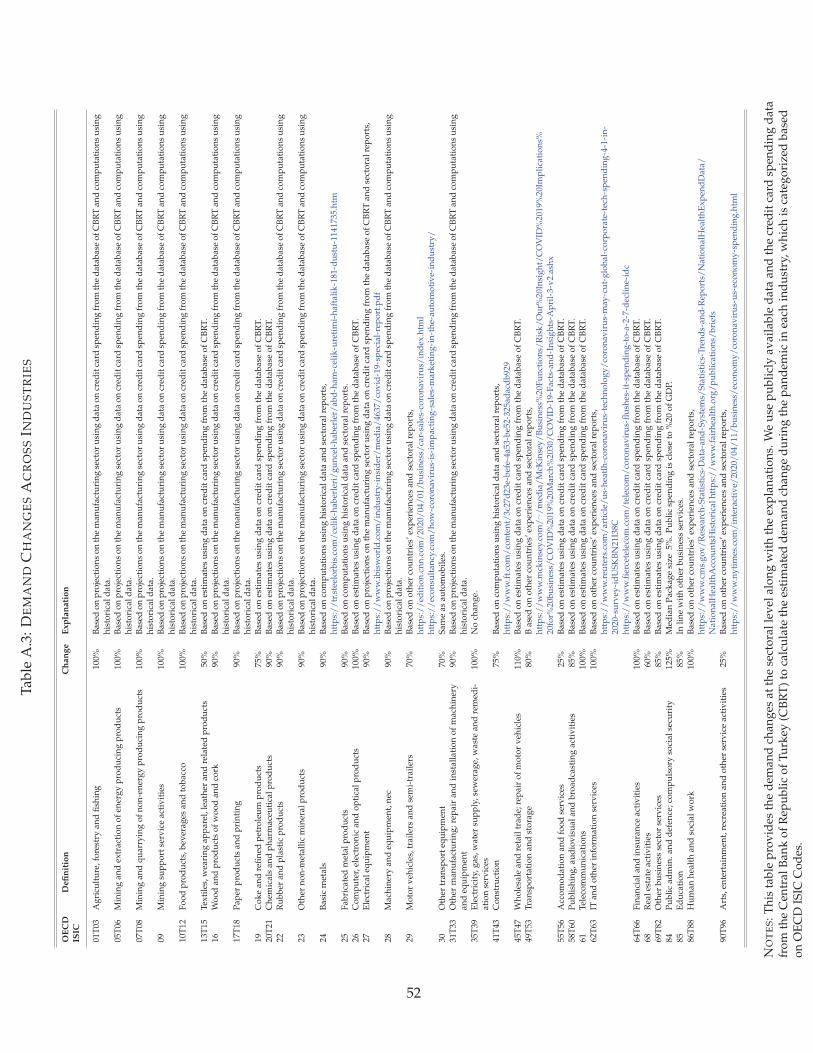
Tab

leA

.3:

DE

MA

ND

CH

AN

GE

SA

CR

OS

SIN

DU

ST

RIE

S

OE

CD

ISIC

Defi

nit

ion

Ch

an

ge

Exp

lan

ati

on

01T

03A

gri

cult

ure

,fo

rest

ryan

dfi

shin

g10

0%B

ased

on

pro

ject

ion

so

nth

em

anu

fact

uri

ng

sect

or

usi

ng

dat

ao

ncr

edit

card

spen

din

gfr

om

the

dat

abas

eo

fC

BR

Tan

dco

mp

uta

tio

ns

usi

ng

his

tori

cal

dat

a.05

T06

Min

ing

and

extr

acti

on

of

ener

gy

pro

du

cin

gp

rod

uct

s10

0%B

ased

on

pro

ject

ion

so

nth

em

anu

fact

uri

ng

sect

or

usi

ng

dat

ao

ncr

edit

card

spen

din

gfr

om

the

dat

abas

eo

fC

BR

Tan

dco

mp

uta

tio

ns

usi

ng

his

tori

cal

dat

a.07

T08

Min

ing

and

qu

arry

ing

of

no

n-e

ner

gy

pro

du

cin

gp

rod

uct

s10

0%B

ased

on

pro

ject

ion

so

nth

em

anu

fact

uri

ng

sect

or

usi

ng

dat

ao

ncr

edit

card

spen

din

gfr

om

the

dat

abas

eo

fC

BR

Tan

dco

mp

uta

tio

ns

usi

ng

his

tori

cal

dat

a.09

Min

ing

sup

po

rtse

rvic

eac

tiv

itie

s10

0%B

ased

on

pro

ject

ion

so

nth

em

anu

fact

uri

ng

sect

or

usi

ng

dat

ao

ncr

edit

card

spen

din

gfr

om

the

dat

abas

eo

fC

BR

Tan

dco

mp

uta

tio

ns

usi

ng

his

tori

cal

dat

a.10

T12

Fo

od

pro

du

cts,

bev

erag

esan

dto

bac

co10

0%B

ased

on

pro

ject

ion

so

nth

em

anu

fact

uri

ng

sect

or

usi

ng

dat

ao

ncr

edit

card

spen

din

gfr

om

the

dat

abas

eo

fC

BR

Tan

dco

mp

uta

tio

ns

usi

ng

his

tori

cal

dat

a.13

T15

Tex

tile

s,w

eari

ng

app

arel

,lea

ther

and

rela

ted

pro

du

cts

50%

Bas

edo

nes

tim

ates

usi

ng

dat

ao

ncr

edit

card

spen

din

gfr

om

the

dat

abas

eo

fC

BR

T.

16W

oo

dan

dp

rod

uct

so

fw

oo

dan

dco

rk90

%B

ased

on

pro

ject

ion

so

nth

em

anu

fact

uri

ng

sect

or

usi

ng

dat

ao

ncr

edit

card

spen

din

gfr

om

the

dat

abas

eo

fC

BR

Tan

dco

mp

uta

tio

ns

usi

ng

his

tori

cal

dat

a.17

T18

Pap

erp

rod

uct

san

dp

rin

tin

g90

%B

ased

on

pro

ject

ion

so

nth

em

anu

fact

uri

ng

sect

or

usi

ng

dat

ao

ncr

edit

card

spen

din

gfr

om

the

dat

abas

eo

fC

BR

Tan

dco

mp

uta

tio

ns

usi

ng

his

tori

cal

dat

a.19

Co

ke

and

refi

ned

pet

role

um

pro

du

cts

75%

Bas

edo

nes

tim

ates

usi

ng

dat

ao

ncr

edit

card

spen

din

gfr

om

the

dat

abas

eo

fC

BR

T.

20T

21C

hem

ical

san

dp

har

mac

euti

cal

pro

du

cts

90%

Bas

edo

nes

tim

ates

usi

ng

dat

ao

ncr

edit

card

spen

din

gfr

om

the

dat

abas

eo

fC

BR

T.

22R

ub

ber

and

pla

stic

pro

du

cts

90%

Bas

edo

np

roje

ctio

ns

on

the

man

ufa

ctu

rin

gse

cto

ru

sin

gd

ata

on

cred

itca

rdsp

end

ing

fro

mth

ed

atab

ase

of

CB

RT

and

com

pu

tati

on

su

sin

gh

isto

rica

ld

ata.

23O

ther

no

n-m

etal

lic

min

eral

pro

du

cts

90%

Bas

edo

np

roje

ctio

ns

on

the

man

ufa

ctu

rin

gse

cto

ru

sin

gd

ata

on

cred

itca

rdsp

end

ing

fro

mth

ed

atab

ase

of

CB

RT

and

com

pu

tati

on

su

sin

gh

isto

rica

ld

ata.

24B

asic

met

als

90%

Bas

edo

nco

mp

uta

tio

ns

usi

ng

his

tori

cal

dat

aan

dse

cto

ral

rep

ort

s,h

ttp

s:/

/tr

.ste

elo

rbis

.co

m/

celi

k-h

aber

leri

/g

un

cel-

hab

erle

r/ab

d-h

am-c

elik

-ure

tim

i-h

afta

lik

-181

-du

stu

-114

1735

.htm

25F

abri

cate

dm

etal

pro

du

cts

90%

Bas

edo

nco

mp

uta

tio

ns

usi

ng

his

tori

cal

dat

aan

dse

cto

ral

rep

ort

s.26

Co

mp

ute

r,el

ectr

on

ican

do

pti

cal

pro

du

cts

100%

Bas

edo

nes

tim

ates

usi

ng

dat

ao

ncr

edit

card

spen

din

gfr

om

the

dat

abas

eo

fC

BR

T.

27E

lect

rica

leq

uip

men

t90

%B

ased

on

pro

ject

ion

so

nth

em

anu

fact

uri

ng

sect

or

usi

ng

dat

ao

ncr

edit

card

spen

din

gfr

om

the

dat

abas

eo

fC

BR

Tan

dse

cto

ral

rep

ort

s,h

ttp

s:/

/w

ww

.ib

isw

orl

d.c

om

/in

du

stry

-in

sid

er/

med

ia/

4637

/co

vid

-19-

spec

ial-

rep

ort

.pd

f28

Mac

hin

ery

and

equ

ipm

ent,

nec

90%

Bas

edo

np

roje

ctio

ns

on

the

man

ufa

ctu

rin

gse

cto

ru

sin

gd

ata

on

cred

itca

rdsp

end

ing

fro

mth

ed

atab

ase

of

CB

RT

and

com

pu

tati

on

su

sin

gh

isto

rica

ld

ata.

29M

oto

rv

ehic

les,

trai

lers

and

sem

i-tr

aile

rs70

%B

ased

on

oth

erco

un

trie

s’ex

per

ien

ces

and

sect

ora

lre

po

rts,

htt

ps:

//

edit

ion

.cn

n.c

om

/20

20/

04/

01/

bu

sin

ess/

car-

sale

s-co

ron

avir

us/

ind

ex.h

tml

htt

ps:

//

eco

nsu

ltan

cy.c

om

/h

ow

-co

ron

avir

us-

is-i

mp

acti

ng

-sal

es-m

ark

etin

g-i

n-t

he-

auto

mo

tiv

e-in

du

stry

/30

Oth

ertr

ansp

ort

equ

ipm

ent

70%

Sam

eas

auto

mo

bil

es.

31T

33O

ther

man

ufa

ctu

rin

g;

rep

air

and

inst

alla

tio

no

fm

ach

iner

yan

deq

uip

men

t90

%B

ased

on

pro

ject

ion

so

nth

em

anu

fact

uri

ng

sect

or

usi

ng

dat

ao

ncr

edit

card

spen

din

gfr

om

the

dat

abas

eo

fC

BR

Tan

dco

mp

uta

tio

ns

usi

ng

his

tori

cal

dat

a.35

T39

Ele

ctri

city

,g

as,

wat

ersu

pp

ly,

sew

erag

e,w

aste

and

rem

edi-

atio

nse

rvic

es10

0%N

och

ang

e.

41T

43C

on

stru

ctio

n75

%B

ased

on

com

pu

tati

on

su

sin

gh

isto

rica

ld

ata

and

sect

ora

lre

po

rts,

htt

ps:

//

ww

w.f

t.co

m/

con

ten

t/3c

27d

23e-

bef

e-4a

53-b

e52-

325a

dac

db

929

45T

47W

ho

lesa

lean

dre

tail

trad

e;re

pai

ro

fm

oto

rv

ehic

les

110%

Bas

edo

nes

tim

ates

usi

ng

dat

ao

ncr

edit

card

spen

din

gfr

om

the

dat

abas

eo

fC

BR

T.

49T

53T

ran

spo

rtat

ion

and

sto

rag

e80

%B

ased

on

oth

erco

un

trie

s’ex

per

ien

ces

and

sect

ora

lre

po

rts,

htt

ps:

//

ww

w.m

ckin

sey.

com

/∼

/m

edia

/M

cKin

sey

/B

usi

nes

s%20

Fu

nct

ion

s/R

isk

/O

ur%

20In

sig

ht/

CO

VID

%20

19%

20Im

pli

cati

on

s%20

for%

20b

usi

nes

s/C

OV

ID%

2019

%20

Mar

ch%

2030

/C

OV

ID-1

9-F

acts

-an

d-I

nsi

gh

ts-A

pri

l-3-

v2.

ash

x55

T56

Acc

om

od

atio

nan

dfo

od

serv

ices

25%

Bas

edo

nes

tim

ates

usi

ng

dat

ao

ncr

edit

card

spen

din

gfr

om

the

dat

abas

eo

fC

BR

T.

58T

60P

ub

lish

ing

,au

dio

vis

ual

and

bro

adca

stin

gac

tiv

itie

s85

%B

ased

on

esti

mat

esu

sin

gd

ata

on

cred

itca

rdsp

end

ing

fro

mth

ed

atab

ase

of

CB

RT

.61

Tel

eco

mm

un

icat

ion

s10

0%B

ased

on

esti

mat

esu

sin

gd

ata

on

cred

itca

rdsp

end

ing

fro

mth

ed

atab

ase

of

CB

RT

.62

T63

ITan

do

ther

info

rmat

ion

serv

ices

100%

Bas

edo

no

ther

cou

ntr

ies’

exp

erie

nce

san

dse

cto

ral

rep

ort

s,h

ttp

s:/

/w

ww

.reu

ters

.co

m/

arti

cle/

us-

hea

tlh

-co

ron

avir

us-

tech

no

log

y/

coro

nav

iru

s-m

ay-c

ut-

glo

bal

-co

rpo

rate

-tec

h-s

pen

din

g-4

-1-i

n-

2020

-su

rvey

-id

US

KB

N21

I38C

htt

ps:

//

ww

w.fi

erce

tele

com

.co

m/

tele

com

/co

ron

avir

us-

flu

shes

-it-

spen

din

g-t

o-a

-2-7

-dec

lin

e-id

c64

T66

Fin

anci

alan

din

sura

nce

acti

vit

ies

100%

Bas

edo

nes

tim

ates

usi

ng

dat

ao

ncr

edit

card

spen

din

gfr

om

the

dat

abas

eo

fC

BR

T.

68R

eal

esta

teac

tiv

itie

s60

%B

ased

on

esti

mat

esu

sin

gd

ata

on

cred

itca

rdsp

end

ing

fro

mth

ed

atab

ase

of

CB

RT

.69

T82

Oth

erb

usi

nes

sse

cto

rse

rvic

es85

%B

ased

on

esti

mat

esu

sin

gd

ata

on

cred

itca

rdsp

end

ing

fro

mth

ed

atab

ase

of

CB

RT

.84

Pu

bli

cad

min

.an

dd

efen

ce;c

om

pu

lso

ryso

cial

secu

rity

125%

Med

ian

Pac

kag

esi

ze5%

.P

ub

lic

spen

din

gis

clo

seto

%20

of

GD

P.85

Ed

uca

tio

n85

%In

lin

ew

ith

oth

erb

usi

nes

sse

rvic

es.

86T

88H

um

anh

ealt

han

dso

cial

wo

rk10

0%B

ased

on

oth

erco

un

trie

s’ex

per

ien

ces

and

sect

ora

lre

po

rts,

htt

ps:

//

ww

w.c

ms.

go

v/

Res

earc

h-S

tati

stic

s-D

ata-

and

-Sy

stem

s/S

tati

stic

s-T

ren

ds-

and

-Rep

ort

s/N

atio

nal

Hea

lth

Ex

pen

dD

ata/

Nat

ion

alH

ealt

hA

cco

un

tsH

isto

rica

lh

ttp

s:/

/w

ww

.fai

rhea

lth

.org

/p

ub

lica

tio

ns/

bri

efs

90T

96A

rts,

ente

rtai

nm

ent,

recr

eati

on

and

oth

erse

rvic

eac

tiv

itie

s25

%B

ased

on

oth

erco

un

trie

s’ex

per

ien

ces

and

sect

ora

lre

po

rts,

htt

ps:

//

ww

w.n

yti

mes

.co

m/

inte

ract

ive/

2020

/04

/11

/b

usi

nes

s/ec

on

om

y/

coro

nav

iru

s-u

s-ec

on

om

y-s

pen

din

g.h

tml

NO

TE

S:

Th

ista

ble

pro

vid

esth

ed

eman

dch

ang

esat

the

sect

ora

lle

vel

alo

ng

wit

hth

eex

pla

nat

ion

s.W

eu

sep

ub

licl

yav

aila

ble

dat

aan

dth

ecr

edit

card

spen

din

gd

ata

fro

mth

eC

entr

alB

ank

of

Rep

ub

lic

of

Tu

rkey

(CB

RT

)to

calc

ula

teth

ees

tim

ated

dem

and

chan

ge

du

rin

gth

ep

and

emic

inea

chin

du

stry

,wh

ich

isca

teg

ori

zed

bas

edo

nO

EC

DIS

ICC

od

es.

52

Table A.4: LIST OF THE LOCKDOWN SECTORS

Panel A: Lockdown Sectors

NACE Rev. 2 Definition

01 Crop and animal production, hunting and related service activities1071 Manufacture of bread; manufacture of fresh pastry goods and cakes1811 Printing of newspapers1920 Manufacture of refined petroleum products21 Manufacture of basic pharmaceutical products and pharmaceutical preparations35 Electricity, gas, steam and air conditioning supply36 Water collection, treatment and supply

4646 Wholesale of pharmaceutical goods4730 Retail sale of automotive fuel in specialised stores4773 Dispensing chemist in specialised stores4774 Retail sale of medical and orthopaedic goods in specialised stores4920 Freight rail transport4941 Freight transport by road5224 Cargo handling53 Postal and courier activities60 Programming and broadcasting activities61 Telecommunications639 Other information service activities75 Veterinary activities86 Human health activities87 Residential care activities

Panel B: Additional Sectors

NACE Rev. 2 Definition

10 Manufacture of food products1722 Manufacture of household and sanitary goods and of toilet requisites463 Wholesale of food, beverages and tobacco

4711 Retail sale in non-specialised stores with food, beverages or tobacco predominating472 Retail sale of food, beverages and tobacco in specialised stores

4781 Retail sale via stalls and markets of food, beverages and tobacco products

NOTES: This table provides the list of the lockdown sectors. We use the decree issued by the Turkish Ministry of Interioron April 10, 2020 to identify these industries. This lockdown was effective for only two days and cover those given inPanel A. We supplement the list with those available in Panel B.

53

Table A.5: CBRT CREDIT CARD SPENDING TITLES CORRESPONDING TO OECD ISIC SECTORS

CBRT Definition OECD ISIC Code

1 Total2 Car Rental 69T823 Car Rental-Sales/Service/Parts 45T474 Petrol Stations 195 Various Food 10T126 Direct Marketing 45T477 Education/Stationary 45T478 Electric & Electronic Goods, Computers 269 Clothing and Accessory 13T1510 Airlines 49T5311 Service 58T60 & 68 & 69T8212 Accomodation 55T5613 Club/Association/ Social Services 55T5614 Casino 55T5615 Jewellery 45T4716 Marketing and Shopping Centers 45T4717 Furnishing and Decoration 31T3318 Contractor Services 41T4319 Health/Health Products/Cosmetics 20T2120 Travel Agencies/Forwarding 69T8221 Insurance 64T6622 Telecommunication 6123 Building Supplies, Hardware, Hard Goods 2524 Food 55T5625 Government/Tax Payments 8426 Private Pensions 64T6627 Others28 E-commerce Transactions 62T6329 Mail or Phone Shopping30 Customs Payments 84

NOTES: This table provides the concordance that we use to match the titles used in the CBRT’s credit card spending datawith the OECD ISIC Codes.

Table A.6: LIST OF THE ACTIVE SECTORS IN PUBLIC ADMINISTRATION DURING FULL LOCKDOWN

Type Size Source

Public (All) 2820095 http://www.sbb.gov.tr/kamu-istihdami/Security 273000 https://tr.wikipedia.org/wiki/Emniyet Genel M%C3%BCd%C3%BCrl%C3%BC%C4%

9F%C3%BCGendarmerie 150000 https://www.jandarma.gov.tr/jandarma-genel-komutanligi-2019-yili-faaliyet-raporuHealth 642184 https://www.saglik.gov.tr/TR,11588/istatistik-yilliklari.html

Share 37.77%

NOTES: This table provides the list of occupations in Public Administration that work during full lockdown, togetherwith the number of people within those occupations. The data sources are provided as well. The share of the activesub-sectors in the entire sector is 37%.

54