COVID‑19 and instability of stock market performance: evidence from the U.S.Hui Hong1,2, Zhicun Bian3 and Chien‑Chiang Lee1,2*

IntroductionThe novel coronavirus 2019 (COVID-19) disease has led to an unprecedented disruption to the U.S. economy and also an unparalleled slump in the U.S. stock market. Typically, a key market-wide circuit breaker designed to prevent the stock market from falling through the floor had been triggered four times in sequence in March 2020. Investors inevitably suffered heavy losses from plunging stock prices. Fears about the crisis and its impact on the global economy rapidly spread to the rest of the world. According to the report ‘Coronavirus: US stocks see worst fall since 1987 from China Daily on the 17th March 2020, after the U.S. market experienced worst point declines in history, global markets saw similar slides. That is, the performance of the U.S. market was a leading indicator of ups and downs of global markets particularly under such circum-stances. This paper thus provides a comprehensive analysis on the association between

Abstract

The effect of COVID‑19 on stock market performance has important implications for both financial theory and practice. This paper examines the relationship between COVID‑19 and the instability of both stock return predictability and price volatility in the U.S over the period January 1st, 2019 to June 30th, 2020 by using the methodolo‑gies of Bai and Perron (Econometrica 66:47–78, 1998. https ://doi.org/10.2307/29985 40; J Appl Econo 18:1–22, 2003. https ://doi.org/10.1002/jae.659), Elliot and Muller (Optimal testing general breaking processes in linear time series models. University of Califor‑nia at San Diego Economic Working Paper, 2004), and Xu (J Econ 173:126–142, 2013. https ://doi.org/10.1016/j.jecon om.2012.11.001). The results highlight a single break in return predictability and price volatility of both S&P 500 and DJIA. The timing of the break is consistent with the COVID‑19 outbreak, or more specifically the stock selling‑offs by the U.S. senate committee members before COVID‑19 crashed the market. Furthermore, return predictability and price volatility significantly increased following the derived break. The findings suggest that the pandemic crisis was associated with market inefficiency, creating profitable opportunities for traders and speculators. Fur‑thermore, it also induced income and wealth inequality between market participants with plenty of liquidity at hand and those short of funds.

Keywords: COVID‑19, Stock returns, Structural breaks, U.S

JEL Classification: C22, G15, G18

Open Access

© The Author(s) 2021. Open Access This article is licensed under a Creative Commons Attribution 4.0 International License, which permits use, sharing, adaptation, distribution and reproduction in any medium or format, as long as you give appropriate credit to the original author(s) and the source, provide a link to the Creative Commons licence, and indicate if changes were made. The images or other third party material in this article are included in the article’s Creative Commons licence, unless indicated otherwise in a credit line to the mate‑rial. If material is not included in the article’s Creative Commons licence and your intended use is not permitted by statutory regulation or exceeds the permitted use, you will need to obtain permission directly from the copyright holder. To view a copy of this licence, visit http://creat iveco mmons .org/licen ses/by/4.0/.

RESEARCH

Hong et al. Financ Innov (2021) 7:12 https://doi.org/10.1186/s40854‑021‑00229‑1 Financial Innovation

*Correspondence: cclee6101@gmail.com 1 Research Center for Central China Economic and Social Development, Nanchang University, Nanchang, Jiangxi, ChinaFull list of author information is available at the end of the article

Page 2 of 18Hong et al. Financ Innov (2021) 7:12

COVID-19 and the instability of the U.S. stock market performance (including both return predictability and price volatility), which serves the interests of investors when making investment decisions during difficult times (Kou et al. 2014, 2021). Facts in the past prove that crises induce risks but also create investment opportunities: stock return predictability and price volatility substantially increase in bad times (e.g., Schwert 1989; Cujean and Hasler 2017; Hong et al. 2018; Liu et al. 2020a; Narayan 2020a, 2020b).

Since the outbreak of COVID-19, there are an increasing number of studies on stock market reactions to the crisis (e.g., Ashraf 2020a, b; Baker et  al. 2020; Lee and Chen 2020; Mazur et al. 2020; Narayan et al. 2020; Topcu and Gulal 2020). The arrived consen-sus is that stock prices severely dropped and price fluctuation greatly enlarged following the occurrence of the pandemic disease. However, those studies did not test whether and when COVID-19 triggered the dramatic changes in stock market performance assum-ing no prior knowledge of the break location. Furthermore, they only focused on price changes and volatility but failed to concern return predictability which is an important theme in the finance literature.

This paper fills the research gap by studying the instability of stock return predictabil-ity and price volatility, and its linkage with COVID-19. Using daily data from January 1st, 2019 to June 30th, 2020 and the structural break tests proposed by Bai and Perron (1998, 2003), Elliot and Mullier (2004) and Xu (2013), we find that there exists a sin-gle break for both S&P 500 and DJIA return prediction models. The break took place in mid-late February, 2020, the timing of which is consistent with the COVID-19 out-break or more specifically the stock selling-offs by the U.S. senate committee members before COVID-19 crashed the market. Furthermore, we also find evidence of a single break in price volatilities of both S&P 500 and DJIA, which occurred on February 21st, 2020, similar to the case of return predictability. The findings of significant increases in both return predictability and price volatility during COVID-19 indicate that the pan-demic created profitable investment opportunities for market participants, with those with plenty of liquidity at hand benefiting most. Fed policy of pumping liquidity to the financial system might have stimulated profitability seeking in the stock market, which may enlarge income and wealth inequality.

The paper thus contributes to the existing literature in two important ways. First, pre-vious studies either use event analyses (i.e., partition the sample to examine the differ-ence of stock market performance across subsamples) or exogenous variable analyses (i.e., take major events as exogenous variables and establish models describing the rela-tionship between market performance and those variables) to determine how stock mar-kets react to external shocks (e.g., Mohanty et al. 2010; Ashraf 2020a, b). This paper tests for structural breaks in return predictive and price volatility models without COVID-19 variables and investigates the linkage between those breaks and COVID-19, thus pro-viding explicit empirical evidence about whether and how public crisis affects market performance. Second, it also adds to the literature by studying stock return predictabil-ity when COVID-19 broke out, thus providing unprecedented evidence that suggests potential investment opportunities for investors.

The rest of the paper proceeds as follows. First, we briefly review the literature. Sec-ond, we describe the data used for empirical analysis. Third, we evaluate the role of COVID-19 on the instability of return predictability and price volatility in the U.S.

Page 3 of 18Hong et al. Financ Innov (2021) 7:12

market, respectively. Finally, we conclude the paper with suggestions to both investors and policy makers.

Literature reviewDetermination of future stock return and volatility

As for prediction, a large literature has identified a number of predictors that are use-ful to predict future stock returns. Those include (but are not limited to) dividend yield and dividend-price ratio (Fama and French 1988; Campell and Shiller 1988), price-earn-ings ratio (Campell and Shiller 1988; Welch and Goyal 2008), short interest rate (Camp-bell 1987; Ang and Bekaert 2007), term and default spreads (Campbell 1987; Fama and French 1989), and consumption-wealth ratio (Lettau and Ludvigson 2001). Besides predictors, forecasting techniques also play an important role in determining forecast accuracy. According to Mallikarjuna and Rao (2019), traditional regression techniques generally outperform others including artificial intelligence and frequency domain mod-els in providing accurate forecasts.

In terms of stock volatility, academic researchers used to make the forecasts by tra-ditional GARCH models using indicators based on the past behavior of stock price and volatility (Gokcan 2000; Emenogu et al. 2020). More recent studies become aware of issues such as parametric assumptions, leverage and asymmetric effects, and power transformations and long memory (e.g., Brooks 2007; Bandi and Reno 2012; Hou 2013). In this paper, we introduce GARCH models for volatility forecasting because we aim to test for the instability of the volatility process, which is primarily built upon those mod-eling techniques.

Major events and stock market performance

Return and price volatility are two important indicators of market performance. Their changes can be divided into two categories: small changes and large jumps/declines (or alternatively structural changes). According to Glosten and Milgorm (1985), the former is triggered by information flows or liquidity shifts while the latter is induced by major events, including financial crises, policy changes and natural disasters. For example, Schwert (2011) shows historically high levels of stock market volatility in the months following the financial crisis in late 2008. By using data of 13 OECD countries over the period from 1972 to 2002, Ioannidis and Kontonikas (2008) find that monetary policy shifts significantly affect stock returns. Landfear et al. (2019) document abnormal nega-tive effects on stock returns due to the U.S. landfall hurricanes.

As a public crisis, COVID-19 is inflicting unprecedented global destructive eco-nomic damage (Phan and Narayan 2020). In a recent pioneer study, Goodell (2020) highlights that COVID-19 may have wide ranging influence on financial sectors including stock markets. Empirical evidence also supports the statement. For exam-ple, based on data of 64 (advanced and emerging) countries over the period Janu-ary 22, 2020 to April 12, 2020, Ashraf (2020a, b) find that stock markets negatively react to COVID-19 and this reaction varies over time depending on the stage of the outbreak. When extending data to 77 countries’ main indices, Liu et al. (2020b) reinforce that the pandemic incurs considerable negative shocks on global stock markets. Topcu and Gulal (2020) draw a similar conclusion when only focusing on

Page 4 of 18Hong et al. Financ Innov (2021) 7:12

emerging markets. Whether the effect of COVID-19 on stock markets is transient or permanent depends on the nature of the markets (Gil-Alana and Claudio-Qui-roga 2020). Although recent literature reports that global stock markets react to the COVID-19 pandemic with negative returns, Ashraf (2020a, b) find uniform reaction across countries: the response is stronger for countries with higher national level uncertainty aversion.

With respect to volatility, Baker et al. (2020) point out that “COVID-19 has resulted in the highest stock market volatility among all recent infectious diseases including the Spanish Flu of 1918”. This is also supported by Baig et al. (2020). Sharma (2020) further shows that COVID-19 has a statistically significant effect on stock volatility, but the impact actually varies with countries involved, with the markets in higher-income countries overreacting in the beginning and bouncing back more rapidly than lower-income countries. Engelhardt et al. (2020), on the other hand, argue that the magnitude of market volatility in reaction to COVID-19 depends on trust: vola-tility is significantly lower in high-trust (including societal trust and trust in the gov-ernment) countries.

Structural break tests

Structural break tests for regression models (such as return prediction models) can be dated back to Chow (1960), who develops an F-test for a single break assuming the date for the break is known. Other tests for a single unknown break are Brown et  al. (1975), Andrews (1993) and Andrews et  al. (1996) for instance. More recent studies extend the prior research to allow for multiple breaks, unit root dynamics, heteroske-dasticity and serial correlation (e.g., Bai and Perron 1997, 1998, 2003; Elliott and Muller 2004; Lee et al. 2021). Empirical investigation based on those recent econometric tech-niques includes Paye and Timmermann (2006), Rapach and Wohar (2006), and Hong et al. (2018). In this paper, we consider the methodology of Bai and Perron (1998, 2003) because it allows us to determine the confidence intervals for the timing of break occur-rence as well as the coefficients around the breakpoints. For robustness, we also include Elliot and Muller (2004) which accommodate for various types of breaks like rare, large breaks as well as those with small, frequent breaks.

There are a large number of studies on tests for structural breaks in volatil-ity. These include the most widely used one which is based on the cumulative sum (CUSUM) of squared series. Numerous researchers have developed and empirically implemented versions of the CUMSUM test (e.g., Inclan and Tiao 1994; Lee and Park 2001; Rapach and Strauss 2008; Xu 2008). They differ in how they deal with asset return features like non-normality and serial dependence. The primary issue of the existing CUSUM-based tests, as argued by Xu (2013), is that they are constructed without any explicit alternative hypotheses. This exposes the tests to criticism for having low power in practice even though they are consistent against a broad range of alternatives. This paper thus uses the methodology of Xu (2013), which specifies an alternative that allows for both smooth and abrupt changes in volatility without compromising the diagnostic ability of the CUSUM-based test. For robustness, we also consider a modified test based on the Lagrange multiplier (LM) principle.

Page 5 of 18Hong et al. Financ Innov (2021) 7:12

DataOur datasets consist of two main U.S. stock market indices and predictor variables of concerns to investors. It should be noted that apart from traditional predictors, we also consider sentiment and technical indicators given their importance especially when crises hit the market (e.g., Wen et al. 2019). Table 1 shows the definition, data availability, and the data source for all variables under investigation.

There are several important observations to be noted. First, daily data are employed for a more precise detection of structural breaks in regression models. Therefore, tra-ditional predictors such as the dividend yield, price-earnings ratio and the consump-tion-wealth ratio and those of interest to investors such as the unemployment rate are not included due to their data frequency. Second, a relatively short period January 1st, 2019 to June 30th, 2020 is introduced because a longer period might increase the power of the test but also introduce undesired noises, which would make our linkage of potential breaks with COVID-19 much harder. Third, the length of lag 1 only is considered as daily stock prices tend to rapidly incorporate publicly available information.

Table 1 Data description

Table 1 shows primary information for both stock index returns and predictor variables. PI = the stock price index adjusted for both dividends and splits; VIX = volatility index. Subscripts t and t − 1 are day t and t − 1 , respectively

Symbol Variable Definition Data availability Data source

RS&P500tDaily Standard and

Poor’s 500 (S&P 500) Stock Index Return

log(PIS&P500t /PIS&P500t−1 ) 01/01/2019–06/30/2020

Yahoo Finance

RDJIAtDaily Dow Jones Indus‑

trial Average (DJIA) Stock Index Return

log(PIDJIAt /PIDJIAt−1 )01/01/2019–

06/30/2020Yahoo Finance

SIUSt−1Daily Lagged Short

Interest Rate3‑Month Treasury Bill

Rate01/01/2019–

06/30/2020Federal Reserve Bank of

St. Louis

TSUSt−1Daily Lagged Term

SpreadDifference between

10‑Year Treasury Bond Rate and 3‑Month Treasury Bill Rate

01/01/2019–06/30/2020

Federal Reserve Bank of St. Louis

DSUSt−1Daily Lagged Default

SpreadDifference between

Moody’s Seasoned Baa and Aaa Corpo‑rate Bond Yields

01/01/2019–06/30/2020

Federal Reserve Bank of St. Louis

CVIXUSt−1Daily Lagged Change

in Chicago Board of Options Exchange (COBE) Volatility Index (VIX)

log(VIXUSt /VIXUSt−1)01/01/2019–

06/30/2020www.Inves ting.com

CTVS&P500t−1

Daily Lagged Change in S&P500 Trading Volume

log(CTVS&P500t /CTVS&P500

t−1 )01/01/2019–06/30/2020

Yahoo Finance

CTVDJIAt−1

Daily Lagged Change in DJIA Trading Volume

log(CTVDJIAt /CTVDJIA

t−1 )01/01/2019–

06/30/2020Yahoo Finance

RS&P500t−1Daily Lagged Standard

and Poor’s 500 (S&P 500) Stock Index Return

log(PIS&P500t−1 /PIS&P500t−2 ) 01/01/2019–06/30/2020

Yahoo Finance

RDJIAt−1Daily Dow Jones Indus‑

trial Average (DJIA) Stock Index Return

log(PIDJIAt−1/PIDJIAt−2 )

01/01/2019–06/30/2020

Yahoo Finance

Page 6 of 18Hong et al. Financ Innov (2021) 7:12

Table  2 illustrates the descriptive analysis of those stock index returns and predic-tor variables. Observations highlight that from January 1st, 2019 to June 30th, 2020 the average index returns were 0.0002 and 0.0001 for S&P 500 and DJIA, respectively. The kurtosis values of the returns (more than 16.0000) indicate that large jumps and extreme movements were prevalent in both markets. This may attribute to the four consecu-tive triggers of the key market-wide circuit breaker on March 9th, 12th, 16th and 18th, 2020. Both the short interest rate and the term spread (also known as indictors for future economic activities) fell below zero and the change in VIX (also referred to as ‘the fear gauge’) dropped to as low as − 0.1156 (compared to its highest level 0.1701) during the same period, indicating potential economic contractions.

COVID‑19 and instability of stock return predictabilityWe begin by investigating the role of COVID-19 on the instability of the U.S. stock return predictability. First, we focus on establishing reasonable regression models to predict future returns. Second, we test for the presence, location and the significance of structural breaks in the return prediction models. Next, we investigate whether the derived breaks can be related to COVID-19.

Stock return predictions

As shown in Table  1, predictor variables available to use for predicting stock index returns RS&P500

t and RDJIAt include SIUSt−1 , TS

USt−1 , DS

USt−1 , CVIX

USt−1 , CTV

S&P500t−1 , CTVDJIA

t−1 ,

RS&P500t−1

and RDJIAt−1

. Before the formal model setup, we test the correlations between all the variables and present the results of the correlation matrix in Table 3. It is apparent that DSUSt−1 , CVIX

USt−1 and Rt−1 have a strong relationship with both index returns.

In order to establish reasonable regression models for stock return predictions, we employ the widely-adopted stepwise methodology embedded with Bayesian Information Criterion (BIC) to select predictor variables (e.g., Hsu et al. 2010; Hong et al. 2018). It should be noted that we aim to establish regression models that can be used to predict stock returns rather than choose the best statistical models for predictions. The proce-dure begins with a constant model. At each step the BIC is computed to compare models with and without a predictor variable and the variable is then added or removed from

Table 2 Summary Statistics: 01/01/2019–06/30/2020

Table 2 reports the mean, standard deviation (STD), minimum (Min), maximum (Max), skewness, kurtosis, and the number of observations (Num of Obs) for both stock index returns and predictor variables over the period January 1st, 2019 to June 30th, 2020

Variable Mean STD Min Max Skewness Kurtosis Number of Obs.

RS&P500 0.0002 0.0078 − 0.0554 0.0389 − 1.0167 16.6603 377

RDJIA 0.0001 0.0083 − 0.0601 0.0467 − 1.0053 17.5810 377

SIUS 1.6079 0.8402 − 0.0460 2.4730 − 0.8568 2.3110 377

TSUS 0.1596 0.2966 − 0.5240 1.1630 0.1647 2.8855 377

DSUS 1.0644 0.2477 0.7900 1.9900 1.6558 5.5371 377

CVIXUS 0.0002 0.0383 − 0.1156 0.1701 1.2662 6.6640 377

CTVS&P500 0.0004 0.0780 − 0.3730 0.2742 − 0.4012 7.2318 377

CTVDJIA 0.0004 0.1010 − 0.4126 0.3744 − 0.1001 5.9482 377

Page 7 of 18Hong et al. Financ Innov (2021) 7:12

the model accordingly. This procedure terminates when no variable can be introduced and eliminated. The final model takes the form given by:

where R = the log of stock index returns as described in Table 1; z = the vector of the constant and predictor variables selected by the stepwise regression. ε = the distur-bance term with mean zero and variance σ 2 . Subscripts t and t − 1 are day t and t − 1 , respectively.

Table 4 provides estimation results for predictive regression models, including the esti-mated coefficients of the selected predictor variables and their standard errors, adjusted R2 and the root mean square errors (RMSEs). To save space, we only report estimates of the final models.

The table highlights the inclusion of DSUSt−1 and RS&P500t−1

in the S&P 500 return model and DSUSt−1 and RDJIA

t−1 in the DJIA return model. The estimated coefficients for both mod-

els are statistically significant at the 1% level with hypothesized signs. For example, the negative coefficients of the lagged return series are consistent with the price pressure

(1)Rt = βzt−1 + εt ,

Table 3 Correlation Matrix: 01/01/2019–06/30/2020

Table 3 reports the pairwise Pearson correlations between all variables over the period from January 1st, 2019 to June 30th, 2020. P values are provided in the parentheses

** and ***indicate significance at the 5% and 1% levels, respectively

Variable RS&P500t

SIUS

t−1TS

US

t−1DS

US

t−1CVIX

US

t−1CTV

S&P500

t−1RS&P500

t−1

Panel A. S&P 500

RS&P500t1.000 0.0018

(0.9725)− 0.0134(0.7962)

0.1100 (0.0330**)

0.1641(0.0014***)

0.0001(0.9980)

− 0.3397(0.0000***)

SIUSt−11.0000 − 0.6905

(0.0000***)− 0.5926(0.0000***)

− 0.0021 (0.9677)

0.0103(0.8427)

0.0136 (0.7930)

TSUSt−11.0000 0.6319

(0.0000***)− 0.0800(0.1216)

− 0.0206(0.6907)

0.0761(0.1408)

DSUSt−11.0000 − 0.1201

(0.0198**)− 0.0337(0.5146)

0.1316(0.0106**)

CVIXUSt−1− 1.0000 0.2235

(0.0000***)− 0.7099(0.0000***)

CTVS&P500t−1

1.0000 − 0.1041(0.0437**)

RS&P500t−11.0000

Variable RDJIAt SI

US

t−1TS

US

t−1DS

US

t−1CVIX

US

t−1CTV

DJIA

t−1RDJIA

t−1

Panel B. DJIA

RDJIAt1.0000 0.0049

(0.9248)− 0.0170

(0.7428)0.1062

(0.0395**)0.1593(0.0019***)

0.0181(0.7271)

− 0.3123(0.0000***)

SIUSt−11.0000 − 0.6905

(0.0000***)− 0.5926(0.0000***)

− 0.0021 (0.9677)

0.0085 (0.8691)

0.0144(0.7802)

TSUSt−11.0000 0.6319

(0.0000***)− 0.0800(0.1216)

− 0.0206(0.6907)

0.0718(0.1605)

DSUSt−11.0000 − 0.1201

(0.0198**)− 0.0395(0.4454)

0.1291(0.0123**)

CVIXUSt−11.0000 0.2608

(0.0000***)− 0.6809(0.0000***)

CTVDJIAt−1

1.0000 − 0.1331(0.0098***)

RDJIAt−11.0000

Page 8 of 18Hong et al. Financ Innov (2021) 7:12

hypothesis that heavy trading of the U.S. index component stocks tends to produce price pressure or excess volatility (Vijh 1994). The adjusted R2 values at a more than 10% level is non-negligible and can have important implications for asset-allocation decisions as the predictable component of stock returns is usually relatively small (Kandel and Stam-baugh 1996). Moreover, these regressions have also reached a local minimum of RMSE. Other predictor variables listed in Table 1 are not included in the final models due to their failure to meet the selection criteria of the stepwise regression. It should also be noted that CVIXUS

t−1 are strongly correlated with RS&P500t−1

and RDJIAt−1

as shown in Table 3 such that only RS&P500

t−1 or RDJIA

t−1 enters the final models based on the information criteria.

The results reinforce those in prior studies that indicate an important role of economic fundamentals in explaining the U.S. stock returns (e.g., Rapach and Wohar 2006; Chang et al. 2019). They also highlight strong autocorrelations in the daily U.S. stock returns, consistent with the literature of short-term stock return behavior (e.g., Avramov et al. 2006; Bogousslavsky 2016).

Being aware of general data problems, we further test to what extent our ordinary least square (OLS) estimates might be affected and also present the results in Table  4. We evaluate the robustness of our results by testing whether parameter estimates change substantially after accounting for the effects of both outliers and heteroskedasticity and serial correlation. The table highlights the robustness of the performance of all predic-tive regression models to potential data issues. The estimated coefficients (i.e.,βS&P500

0

,βS&P5001

,βS&P5002

,βDJIA0

, βDJIA1

and βDJIA2

) remain significant at the same statistical level and the RMSE for each model becomes much smaller, suggesting that our OLS estimates

Table 4 Estimation Results of  Stepwise Predictive Regression Models and  Robustness of Parameter Estimates: 01/01/2019–06/30/2020

Table 4 reports both estimation and robust estimation results of the final predictive regression models determined by the BIC over the period January 1st, 2019 to June 30th, 2020a Outlier robust statistics are obtained using iteratively reweighted lease squares with a bi‑square weighting functionb The Newey‑West statistics are used as the heteroskedasticity and serial correlation robust statistics, where the lag calculated as 4 ∗ ( N

100)2/9

is introduced to correct for serial correlation. Standard errors are provided in the parentheses

** and *** indicate significance at the 5% and 1% levels, respectively

Least-Square Regression Statistics

Outlier Robust Statisticsa

Heteroskedasticity and Serial Correlation Statisticsb

Estimate Adjusted R2

RMSE Estimate Adjusted R2

RMSE Estimate Adjusted R2

RMSE

Model I: RS&P500t = βS&P5000 + βS&P500

1 DSUSt−1 + βS&P5002 RS&P500t−1 + εt

βS&P5000

− 0.0050 (0.0017***)

0.1352 0.0073 − 0.0035 (0.0008***)

0.1905 0.0037 − 0.0050 (0.0021**) 0.1352 0.0073

βS&P5001

0.0050 (0.0015***)

0.0043 (0.0008***)

0.0050 (0.0020**)

βS&P5002

− 0.3608 (0.0485***)

− 0.1384 (0.0254***)

− 0.3608 (0.1054***)

Model II:RDJIAt = βDJIA0 + βDJIA

1 DSUSt−1 + βDJIA

2RDJIAt−1 + εt

βDJIA0

− 0.0052 (0.0018***)

0.1146 0.0079 − 0.0035 (0.0009***)

0.1322 0.0038 − 0.0052 (0.0021**) 0.1146 0.0079

βDJIA1

0.0050 (0.0017***)

0.0042 (0.0008***)

0.0050 (0.0022**)

βDJIA2

− 0.3316 (0.0490***)

− 0.2354 (0.0248***)

− 0.3316 (0.1022***)

Page 9 of 18Hong et al. Financ Innov (2021) 7:12

barely suffer from the outlier effect. With respect to the heteroskedasticity and serial correlation, both S&P 500 and DJIA return models are more or less affected: for instance, the standard error is 0.0020 (0.0022) for βS&P500

1 ( βDJIA

1 ), leading to a decrease in the sig-

nificance of the coefficient from 1% to 5%. However, the models remain competitive in forecasting as the coefficients are still important at the conventional level.

Overall, the results suggest that the predictive regression models derived is reason-able for predicting the U.S. stock returns, with non-significant changes in parameter estimates after accounting for potential data problems. Next section turns to whether structural breaks exist and how they may affect model parameters.

Tests for breaks and their significance

As mentioned previously, we introduce Bai and Perron (1998, 2003) and Elliot and Mul-lier (2004) to test for unknown structural breaks. The former enables estimation of breakpoints and statistical analysis of the resulting estimators whereas the latter dis-plays excellent properties in the presence of persistence (given the non-stationarity of the default spread in the final regression models). In our implementation, we allow all coefficients to change at each break since there is no strong reason to believe that any coefficient involved should be immune from shifts.

Table 5 reports the results of various tests for structural breaks which allow for serial correlation, different variances of the errors and trending regressors as well as those for the true number of breaks. The selection of trimming percentages ( π ) is vital to break test results since a small π can cause substantial size distortions while a large π can sharply reduce the combinations of breakpoints allowed. Usually, there are five options for πs : 5%, 10%, 15%, 20%, 25% (Bai and Perron 1998). We set the trimming percent-age,π , to 20% and 25%, allowing for 3 breaks ( m = 3 ) and 2 breaks ( m = 2 ), respectively given the relatively short sample period under studied. These correspond to a minimum window of approximately 94 and 126 days between breaks for our datasets starting from January 1st, 2019.

As expected, the statistics of the SupF(1) test, double maximum tests, SupFt(1|0) test and the J -test are all significant for both π = 20% and π = 25% , suggesting the presence of structural breaks (highly likely a break). Together with the evidence of the BIC and the SM for the number of true breaks, we conclude with one-break prediction models for both S&P 500 and DJIA returns. These findings reinforces those in prior studies that predictive regression models are characterized by structural instability (e.g., Rapach and Wohar 2006; Paye and Timmermann 2006; Hong et al. 2018).

Although the hypothesis tests above suggest statistical significance of instability, they alone cannot reveal the economic significance of the break. To this end, we re-estimate both S&P 500 and DJIA return models in different regimes partitioned by the derived break above. Table  6 reports the estimated coefficients and their standard errors, adjusted R2 , and also the estimated breakpoint as well as its 90% confidence interval.

The regressions reveal several interesting results. Most notably, the predictive regression coefficients as well as the adjusted R2 values of both S&P 500 and DJIA return models change substantially following the break. For instance, in the case of π = 0.20 , the estimated coefficient of DSUSt−1 for Model I was 0.0023 in regime 1 (Janu-ary 1st, 2019 to February 19th, 2020). It increased to 0.0166 with significance at the

Page 10 of 18Hong et al. Financ Innov (2021) 7:12

Tabl

e 5

Bai a

nd P

erro

n (1

998,

200

3) a

nd E

lliot

and

 Mue

ller (

2004

)’ Te

st S

tati

stic

s fo

r Bre

aks

and 

Mod

el S

elec

tion

: 01/

01/2

019–

06/3

0/20

20

Tabl

e 5

repo

rts

the

resu

lts o

f var

ious

test

for s

truc

tura

l bre

aks

in b

oth

S&P

500

and

DJI

A re

turn

mod

els

and

thos

e fo

r the

num

ber o

f tru

e br

eaks

ove

r the

per

iod

Janu

ary

1st,

2019

to Ju

ne 3

0th,

202

0. T

he S

upF

stat

istic

s ar

e us

ed to

test

the

hypo

thes

is o

f no

stru

ctur

al b

reak

aga

inst

the

one‑

side

d (u

pper

‑tai

l) al

tern

ativ

e of

m =

k (k

is a

pre

defin

ed n

umbe

r). T

he d

oubl

e m

axim

um s

tatis

tics

and

the

J‑te

st s

tatis

tic a

re u

sed

to te

st h

ypot

hesi

s of

no

stru

ctur

al b

reak

aga

inst

the

one‑

side

d (u

pper

‑tai

l) al

tern

ativ

e of

an

unkn

own

num

ber o

f bre

aks.

The SupFT(l+

1|l) s

tatis

tics

have

the

null

hypo

thes

is o

f l b

reak

s ag

ains

t the

one

‑sid

ed (u

pper

‑tai

l) al

tern

ativ

e of

l+

1 br

eaks

. The

Bay

esia

n in

form

atio

n cr

iterio

n (B

IC) (

Yao

1988

), a

mod

ified

Sch

war

z cr

iterio

n (L

WZ)

(Liu

et a

l. 19

97) a

nd th

e se

quen

tial m

etho

d (S

M) (

Bai a

nd P

erro

n 19

98) a

re u

sed

to te

st th

e nu

mbe

r of t

rue

brea

ks.

The SupFT(l+

1|l) t

est i

n th

e se

quen

tial c

onte

xt is

diff

eren

t fro

m th

e se

quen

tial m

etho

d be

caus

e th

e fir

st l

brea

ks a

re n

ot n

eces

saril

y th

e gl

obal

min

imiz

ers

of th

e su

m o

f squ

ared

resi

dual

s. Th

e st

atis

tics

allo

w fo

r the

po

ssib

ility

of h

eter

osce

dast

icity

and

ser

ial c

orre

latio

n in

the

erro

rs. T

he h

eter

osce

dast

icity

and

aut

ocor

rela

tion

cons

iste

nt c

ovar

ianc

e m

atrix

is c

onst

ruct

ed fo

llow

ing

And

rew

s (1

991)

and

And

rew

s an

d M

onah

an (1

992)

us

ing

a qu

adra

tic k

erne

l with

aut

omat

ic b

andw

idth

sel

ectio

n ba

sed

on a

firs

t ord

er V

ecto

r Aut

o‑re

gres

sion

(VA

R (1

)) ap

prox

imat

ion.

The

aut

ocor

rela

tion

from

the

resi

dual

s is

rem

oved

als

o us

ing

a VA

R (1

)

* an

d **

indi

cate

sig

nific

ance

at t

he 1

0% a

nd 5

% le

vels

, res

pect

ivel

y

SupF

(1)

SupF

(2)

SupF

(3)

UD

max

aWD

max

SupF

T(1|

0)Su

pFT(

2|1)

SupF

T(3|

2)J-S

tat

BIC

LWZ

SM

Pane

l A: π

=20%,m

=3breaks

Mod

el I:

RS&P500

t=

βS&P500

0+

βS&P500

1DSUS

t−1+

βS&P500

2RS&P500

t−1

+εt

8.6

434**

5.52

984.

2090

8.64

34**

8.64

34**

7.47

33*

3.42

790.

0000

− 1

6.97

66**

10

1

Mod

el II

: RDJIA

t=

βDJIA

0+

βDJIA

1DSUS

t−1+

βDJIA

2RDJIA

t−1+

εt

7.4

514*

5.14

303.

6911

7.45

14*

7.45

14*

6.97

66*

5.09

300.

2501

− 1

3.89

49*

10

1

Pane

l B: π

=25%,m

=2breaks

Mod

el I:

RS&P500

t=

βS&P500

0+

βS&P500

1DSUS

t−1+

βS&P500

2RS&P500

t−1

+εt

7.9

936*

5.10

09/

7.99

36*

7.99

36*

7.56

32*

3.45

04–

− 1

4.13

11*

10

1

Mod

el II

: RDJIA

t=

βDJIA

0+

βDJIA

1DSUS

t−1+

βDJIA

2RDJIA

t−1+

εt

7.3

832*

5.16

63/

7.38

32*

7.38

32*

6.97

66*

5.13

07–

− 1

3.80

12*

10

1

Page 11 of 18Hong et al. Financ Innov (2021) 7:12

Tabl

e 6

Esti

mat

ion

Resu

lts

of M

ulti

ple

Regi

me

Regr

essi

on M

odel

s: 0

1/01

/201

9–06

/30/

2020

Tabl

e 6

repo

rts

leas

t‑sq

uare

est

imat

ion

resu

lts o

f bot

h S&

P 50

0 an

d D

JIA

retu

rn m

odel

s in

diff

eren

t reg

imes

bas

ed o

n th

e de

rived

bre

ak o

ver t

he p

erio

d Ja

nuar

y 1s

t, 20

19 to

June

30t

h, 2

020.

Sta

ndar

d er

rors

in p

aren

thes

es

are

New

ey‑W

est s

tand

ard

erro

rs a

djus

ted

for h

eter

oske

stic

ity a

nd s

eria

l cor

rela

tion.

90%

con

fiden

ce in

terv

al fo

r the

bre

akpo

int i

s re

port

ed in

the

brac

ket

* an

d **

*ind

icat

e si

gnifi

canc

e at

the

10%

and

1%

leve

ls, r

espe

ctiv

ely

Regi

me

1Re

gim

e 2

(1)

(2)

(3)

(4)

(5)

(6)

Estim

ate

Adj

uste

d R2

Brea

kpoi

ntEs

timat

eA

djus

ted R2

Brea

kpoi

nt

Pane

l A:π

=0.20,m

=3breaks

Mod

el I:

RS&P500

t=

βS&P500

0+

βS&P500

1DSUS

t−1+

βS&P500

2RS&P500

t−1

+εt

βS&P500

0−

0.0

017

(0.0

014)

0.00

6502

/20/

2020

[01/

02/2

020–

02/2

5/20

20]

− 0

.023

2 (0

.007

6***

)0.

2488

–

βS&P500

10.

0023

(0.0

015)

0.01

66 (0

.005

4***

)

βS&P500

2−

0.0

973

(0.0

585*

)−

0.4

766

(0.1

108*

**)

Mod

el II

: RDJIA

t=

βDJIA

0+

βDJIA

1DSUS

t−1+

βDJIA

2RDJIA

t−1+

εt

βDJIA

0−

0.0

023

(0.0

015)

0.01

2402

/21/

2020

[12/

20/2

019–

02/2

5/20

20]

− 0

.024

4 (0

.008

5***

)0.

2075

–

βDJIA

10.

0027

(0.0

015*

)0.

0173

(0.0

060*

**)

βDJIA

2−

0.1

170

(0.0

635*

)−

0.4

333

(0.1

158*

**)

Pane

l B:π

=0.25,m

=2breaks

Mod

el I:

RS&P500

t=

βS&P500

0+

βS&P500

1DSUS

t−1+

βS&P500

2RS&P500

t−1

+εt

βS&P500

0−

0.0

017

(0.0

015)

0.00

6302

/14/

2020

[12/

17/2

019–

02/2

0/20

20]

− 0

.020

8 (0

.006

9***

)0.

2367

–

βS&P500

10.

0023

(0.0

015)

0.01

50 (0

.004

7***

)

βS&P500

2−

0.0

963

(0.0

586)

− 0

.468

8 (0

.111

7***

)

Mod

el II

:RDJIA

t=

βDJIA

0+

βDJIA

1DSUS

t−1+

βDJIA

2RDJIA

t−1+

εt

βDJIA

0−

0.0

021

(0.0

016)

0.01

1202

/14/

2020

[12/

04/2

019–

02/1

9/20

20]

− 0

.021

4 (0

.007

6***

)0.

1963

–

βDJIA

10.

0026

(0.0

016)

0.01

53 (0

.005

4***

)

βDJIA

2−

0.1

157

(0.0

638*

)−

0.4

235

(0.1

149*

**)

Page 12 of 18Hong et al. Financ Innov (2021) 7:12

1% level when one moves to regime 2 (February 20th, 2020 to June 30th, 2020). The adjusted R2 value was 0.0065 before the break and increased substantially to 0.2488 afterwards. While some of this variation can be clearly attributed to sampling vari-ation due to sometimes large standard errors, this does not conceal the fact that the derived break in the regression models tends to be sufficiently large that it is of sub-stantial economic interest. It should also be noted that parameter specification has little impact on the break location: the breakpoint (02/20/2020 or 02/21/2020) when π = 0.20 is quite close to (02/14/2020) when π = 0.25 . The difference is actually induced by a minimum window allowed between each break.

Nature of the break

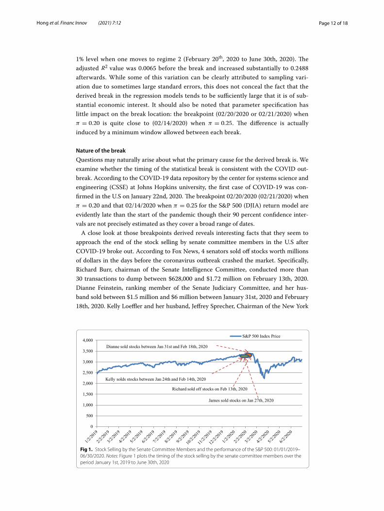
Questions may naturally arise about what the primary cause for the derived break is. We examine whether the timing of the statistical break is consistent with the COVID out-break. According to the COVID-19 data repository by the center for systems science and engineering (CSSE) at Johns Hopkins university, the first case of COVID-19 was con-firmed in the U.S on January 22nd, 2020. The breakpoint 02/20/2020 (02/21/2020) when π = 0.20 and that 02/14/2020 when π = 0.25 for the S&P 500 (DJIA) return model are evidently late than the start of the pandemic though their 90 percent confidence inter-vals are not precisely estimated as they cover a broad range of dates.

A close look at those breakpoints derived reveals interesting facts that they seem to approach the end of the stock selling by senate committee members in the U.S after COVID-19 broke out. According to Fox News, 4 senators sold off stocks worth millions of dollars in the days before the coronavirus outbreak crashed the market. Specifically, Richard Burr, chairman of the Senate Intelligence Committee, conducted more than 30 transactions to dump between $628,000 and $1.72 million on February 13th, 2020. Dianne Feinstein, ranking member of the Senate Judiciary Committee, and her hus-band sold between $1.5 million and $6 million between January 31st, 2020 and February 18th, 2020. Kelly Loeffler and her husband, Jeffrey Sprecher, Chairman of the New York

0

500

1,000

1,500

2,000

2,500

3,000

3,500

4,000S&P 500 Index Price

Richard sold off stocks on Feb 13th, 2020

Dianne sold stocks between Jan 31st and Feb 18th, 2020

Kelly solds stocks between Jan 24th and Feb 14th, 2020

James sold stocks on Jan 27th, 2020

Fig 1. Stock Selling by the Senate Committee Members and the performance of the S&P 500: 01/01/2019–06/30/2020. Notes: Figure 1 plots the timing of the stock selling by the senate committee members over the period January 1st, 2019 to June 30th, 2020

Page 13 of 18Hong et al. Financ Innov (2021) 7:12

Stock Exchange, sold stocks between January 24th, 2020 and February 14th, 2020, worth a total between $1.2 million and $3.1million. James Inhofe sold as much as $400,000 on January 27th, 2020. Figure 1 further visualizes the timing of the stock selling by the senate committee members. It is apparent that the market plunged immediately after those senators dumped their stocks. This further indicates that information asymmetry existed between government bureaucrats and the public. Bureaucrats have information advantage, enabling them to successfully reduce the likelihood of huge losses during the COVID-19 crisis.

Overall, we find that stock return predictability was subject to a structural break which can be ascribed to COVID-19 during the period under investigation. Moreover, the pre-dictability significantly increased after the outbreak of the pandemic crisis. According to Cujean and Hasler (2017), as economic conditions deteriorated, difference in inves-tors’ learning speed increased. Investors’ opinions eventually polarized, causing returns to react to past information.

The findings have vast implications for academic researchers, investors and policy makers. First, COVID-19 is an important cause of market inefficiency, implying signifi-cant return predictability and existence of profitable opportunities for traders and spec-ulators. The selling-offs by insiders provides clues to market timing. Second, profitable opportunities will benefit those who have plenty of liquidity at hand. Third, Fed policy of pumping liquidity into the financial system may have stimulated profitability seeking in the stock market, which may enlarge income and wealth inequality.

COVID‑19 and instability of price volatilityIn this section, we turn to studying the characteristics of price volatility in the COVID-19 context. As with return predictability, first, we attempt to establish reasonable models for modeling price volatility. Second, we focus on testing for the presence, location and

-0.0800

-0.0600

-0.0400

-0.0200

0.0000

0.0200

0.0400

0.0600S&P500 Return

-0.0800

-0.0600

-0.0400

-0.0200

0.0000

0.0200

0.0400

0.0600DJIA Return

Fig 2. Time Series Plots: 01/01/2019–06/30/2020. Notes: Figure 2 plots the time series of both S&P 500 and DJIA for the period January 1st, 2019 to June 30th, 2020

Table 7 Tests for ARCH Effect: 01/01/2019–06/30/2020

Table 7 reports statistics of ARCH effect for both S&P 500 and DJIA over the period January 1st, 2019 to June 30th, 2020. ARCH lags are determined by BIC

***indicates significance at the 1% level

Return ARCH (15) Statistics Return ARCH (15) Statistics

RS&P500t164.1490*** RDJIAt

158.4570***

Page 14 of 18Hong et al. Financ Innov (2021) 7:12

the significance of structural breaks in volatility models. Third, we examine the linkage between the derived breaks and COVID-19.

Price volatility modeling

Before the formal model set up, we investigate stock return behavior for the period studied. Figure 2 plots return series of both S&P 500 and DJIA. It is apparent that large or small changes in prices tend to cluster together, resulting in the persistence of these magnitudes of price changes. Supportive evidence is from the tests for ARCH effect (lag 15) in Table 7: statistics are significant at the 1% level for both return series, indicating potential high-level ARCH effect, i.e., GARCH effect.

The GARCH model involved is then given by:

where σ = non-stationary unconditional variance; ε = potential conditional hetero-scedasticity. R is the same as in Eq. (1). σt is a deterministic function of t and εt sat-isfies E(εt) = 0 and E

(ε2t)= 1 . To determine the orders of the GARCH models in Eq.

(2), we consider several potential possibilities (Mcmillan and Speight 2004) and select the orders by BIC. Table  8 shows that the BIC values increase as orders of the mod-els become larger, thus supporting GARCH (1,1) as the optimal model for describing the volatility process. This is consistent with Ashely and Patterson (2010) who find that GARCH (1,1) is in general adequate for modeling daily price volatility.

Tests for breaks and their significance

As mentioned previously, we introduce Xu (2013) to test for unknown structural breaks in price volatility, which accommodates the stylized facts that previous studies always

(2)Rt = σtεt ,

σ 2t = α0 + α1ε

2t−1 + · · · + αqε

2t−q + β0 + β1σ

2t−1 + · · · + βpσ

2t−p,

Table 8 Tests for GARCH effect: 01/01/2019–06/30/2020

Table 8 displays results of tests for the GARCH effect for both S&P 500 and DJIA over the period January 1st, 2019 to June 30th, 2020. L and BIC are presented in log values

P values are provided in the parentheses

** and *** indicate significance at the 5% and 1% levels, respectively

α0 α1 α2 β1 β2 L BIC

Panel A: S&P 5000

GARCH (1,1) 0.0000 (0.0000***)

0.2642 (0.0038***)

– 0.7356 (0.0018***)

– 1503.0000 − 5.9455

GARCH (2,1) 0.0000 (0.0000***)

0.1810 (0.0104**)

0.1606 (0.0093***)

0.6582 (0.0011***)

– 1504.5000 − 5.8902

GARCH (2,2) 0.0000 (0.0000***)

0.1803 (0.0085***)

0.3224 (0.0040***)

0.0833 (0.0011***)

0.4138 (0.0011***)

1505.2000 − 5.8865

Panel B: DJIA

GARCH (1,1) 0.0000 (0.0000***)

0.2477 (0.0041***)

– 0.7521 (0.0021***)

– 1486.7000 − 5.9201

GARCH (2,1) 0.0000 (0.0000***)

0.1409 (0.0051***)

0.1709 (0.0049***)

0.6835 (0.0088 ***)

– 1488.5000 − 5.8764

GARCH (2,2) 0.0000 (0.0000***)

0.1383 (0.0016***)

0.3316 (0.0195**)

0.0949 (0.0073***)

0.4350 (0.0030***)

1489.4000 − 5.8658

Page 15 of 18Hong et al. Financ Innov (2021) 7:12

lack explicit alternative hypotheses, potentially leading to lower power of tests in prac-tice. Table 9 reports the results for both modified CUSUM and LM tests ( Q and L statis-tics, respectively) for the presence and the number of breaks.

The table highlights that structural breaks are present in volatilities of S&P 500 and DJIA: both modified CUSUM and LM tests reject the constant variance hypothesis at 5% level when cross validated bandwidths are used. Further investigation indicates a sin-gle break with its location around February 21st, 2020, which is similar to the derived break in return predictability.

Figure 3 plots the difference of the realized volatility between two subsamples parti-tioned (i.e. volatility of subsample 1 minus subsample 2) at a given date. Assume that the minimum length of time to compute volatility is one month. The sample period now becomes February 1st, 2019 to May 31st, 2020. It is apparent that the difference of the volatility between subsamples arrives at its maximum (0.0115 for S&P 500 and 0.0126 for DJIA) when the derived break above is used for sample partition. In other words, volatility significantly increased during the period after the break.

Nature of the break

Similar to the case of return predictability, we argue that the timing of the statistical break that took place on February 21st, 2020 is consistent with the COVID-19 outbreak. More specifically, the break occurrence followed closely to the stock selling-offs by the senate committee members in the U.S before COVID-19 crashed the market.

Table 9 Xu (2013)’s Test Statistics for Breaks: 01/01/2019–06/30/2020

Table 9 reports the results of modified CUSUM and LM tests for structural breaks in volatilites of both S&P 500 and DJIA over the period January 1st, 2019 to June 30th, 2020. The modified CUSUM test allows for multiple structural breaks while the modified LM test only allows for a single break. The bandwidth is selected by cross validation. Q is the modified CUSUM test statistic and L is the modified LM test statistic

**indicates significance at the 5% level

Model Q Statistic L Statistic Breakpoint No of Obs.

Panel A: S&P 500

GARCH (1,1) 1.3766** 9.8543** 2020.02.21 377

Panel B: DJIA

GARCH (1,1) 1.3699** 9.7405** 2020.02.21 377

-0.0040

0.0000

0.0040

0.0080

0.0120

0.0160Volatility Difference for S&P500

02/21/2020 Break

-0.0020

0.0020

0.0060

0.0100

0.0140Volatility Difference for DJIA

02/21/2020 Break

Fig 3. Difference of Volatility between Subsamples: 02/01/2019–05/31/2020. Notes: Figure 3 plots the difference of the realized volatility between two subsamples partitioned at a given date

Page 16 of 18Hong et al. Financ Innov (2021) 7:12

As with Geanakoplos (2003) who argues that bad news tends to cause panic among investors such that a crisis is usually accompanied by high volatility, COVID-19 creates better investment opportunities for investors with volatility timing ability (especially those who have plenty of liquidity at hand) than the public. This however may enlarge income and wealth inequality.

ConclusionIn this paper we examine the association between COVID-19 and the instability of the U.S. stock market performance (i.e., return predictability and price volatility). Using daily data from January 1st, 2019 to June 30th, 2020 and methodologies developed by Bai and Perron (1998, 2003), Elliot and Mullier (2004) and Xu (2013), we find that return predictability and price volatility of both S&P 500 and DJIA underwent a single struc-tural break. The break can be related to COVID-19 or more specifically the stock sell-ing-offs by the U.S. senate committee members before COVID-19 crashed the market. Moreover, both return predictability and price volatility increased significantly after the derived break.

Important implications are provided as follows. On one hand, crises may be associated with opportunities. COVID-19 is an important cause for market inefficiency, creating profitable opportunities for traders and speculators. Rational investors seeking to maxi-mize returns may need to pay close attention to insider trading before taking any deci-sions in the stock market. On the other hand, crises may also induce income and wealth inequality as market participants with plenty of liquidity at hand can seek for profitabil-ity in the stock market.

Future research avenues might consider testing whether the structural shift is tran-sient or permanent given its important policy implications. Furthermore, extending the analysis to more countries and comparing their similarities and differences would offer more insightful outcomes.AcknowledgementsWe would like to thank the Editor and three anonymous referees for their highly constructive comments.

Authors’ contributionsHH was writing responsible for conceptualization, investigation, and writing of original draft and analysis. ZB collected, analyzed and interpreted the data regarding stock price index and predictor variables. C‑CL was responsible for the investigation and formal analysis. All authors read and approved the final manuscript.

FundingThis research was supported by the Social Science Foundation of Jiangxi Province (Grant No: 20YJ09) and the National Social Science Foundation of China (Grant No: 17ZDA037).

Availability of data and materialsData available from the authors upon request.

Ethical approvalThis article does not contain any studies with human participants or animals performed by any of the authors.

Competing interestsAll authors declare that they have no competing interests.

Author details1 Research Center for Central China Economic and Social Development, Nanchang University, Nanchang, Jiangxi, China. 2 School of Economics and Management, Nanchang University, Nanchang, Jiangxi, China. 3 School of Finance, Nanjing University of Finance and Economics, Nanjing, Jiangsu, China.

Received: 6 December 2020 Accepted: 15 February 2021

Page 17 of 18Hong et al. Financ Innov (2021) 7:12

ReferencesAndrews DWK (1991) Heteroskedasticity and autocorrelation consistent covariance matrix estimation. Econometrica

59:817–858Andrews DWK (1993) Tests for parameter instability and structural change with unknown change point. Econometrica

61:821–858Andrews DWK, Monahan JC (1992) An improved heteroskedasticity and autocorrelation consistent covariance matrix

estimator. Econometrica 60:953–966Andrews DWK, Lee I, Ploberger W (1996) Optimal change point tests for normal linear regression. J Econ 70:9–38. https ://

doi.org/10.1016/0304‑4076(94)01682 ‑8Ang A, Bekaert G (2007) Stock return predictability: Is it there? Rev Finance Stud 20:651–707. https ://doi.org/10.1093/rfs/

hhl02 1Ashley RA, Patterson DM (2010) A test of the GARCH (1,1) specification for daily stock returns. Macroecon Dyn 14:137–

144. https ://doi.org/10.1017/S1365 10051 00000 15Ashraf BN (2020a) Stock market’s reaction to COVID‑19: Cases or fatalities? Res Int Bus Finance 54:1–7. https ://doi.

org/10.1016/j.ribaf .2020.10124 9Ashraf BN (2020b) Stock markets’ reaction to COVID‑19: Moderating role of national culture. Finance Res Lett (forthcom‑

ing). https ://doi.org/10.1016/j.frl.2020.10185 7Avramov D, Chordia T, Goyal A (2006) Liquidity and autocorrelation in individual stock returns. J Finance 61:2365–2394.

https ://doi.org/10.1111/j.1540‑6261.2006.01060 .xBai JS, Perron P (1997) Estimation of a change point in multiple regression models. Rev Econ Stat 79:551–563. https ://doi.

org/10.1162/00346 53975 57132 Bai JS, Perron P (1998) Estimating and testing linear models with multiple structural changes. Econometrica 66:47–78.

https ://doi.org/10.2307/29985 40Bai JS, Perron P (2003) Computation and analysis of multiple structural change models. J Appl Econ 18:1–22. https ://doi.

org/10.1002/jae.659Baig AS, Butt HA, Haroon O, Rizvi SAR (2020) Deaths, panic, lockdowns and US equity markets: The case of COVID‑19

pandemic. Finance Research Letters (Forthcoming).Baker S, Bloom N, Davis SJ, Kost K, Sammon M, Viratyosin T (2020) The unprecedented stock market reaction to COVID‑19.

Rev Asset Pricing Stud 10:742–758. https ://doi.org/10.1093/rapst u/raaa0 08Bandi FM, Reno R (2012) Time‑varying leverage effects. J Econ 169:94–113. https ://doi.org/10.1016/j.jecon om.2012.01.010Bogousslavsky V (2016) Infrequent rebalancing, return autocorrelation, and seasonality. J Finance 71:2967–3006. https ://

doi.org/10.1111/jofi.12436 Brooks R (2007) Power arch modeling of the volatility of emerging equity markets. Emerg Markets Rev 8:124–133. https ://

doi.org/10.1016/j.emema r.2007.01.002Brown RL, Durbin J, Evans JM (1975) Techniques for testing the constancy of regression relationships over time. J Roy Stat

Soc 37:149–192. https ://doi.org/10.1111/j.2517‑6161.1975.tb015 32.xCampbell JY (1987) Stock returns and the term structure. J Finance Econ 18:373–399. https ://doi.org/10.1016/0304‑

405x(87)90045 ‑6Campbell JY, Shiller RJ (1988) Stock prices, earnings, and expected dividends. J Finance 43:661–676. https ://doi.

org/10.1111/j.1540‑6261.1988.tb045 98.xChang TY, Gupta R, Majumdar A, Pierdzioch C (2019) Predicting stock market movements with a time‑varying consump‑

tion‑aggregate wealth ratio. Inte Rev Econ Finance 59:458–467. https ://doi.org/10.1016/j.iref.2018.10.009Chow GC (1960) Tests of equality between subsets of coefficients in two linear regression models. Econometrica

28:591–605. https ://doi.org/10.2307/19101 33Cujean J, Hasler M (2017) Why does return predictability concentrate in bad times? J Finance 72:2717–2757. https ://doi.

org/10.1111/jofi.12544 Elliot G, Mueller U (2004) Optimal testing general breaking processes in linear time series models. University of California

at San Diego Economic Working Paper.Emenogu NG, Adenomon MO, Nweze NO (2020) On the volatility of daily stock returns of total Nigeria Plc: Evidence from

GARCH models, value‑at‑risk and backtesting. Innov 6:1–25. https ://doi.org/10.1186/s4085 4‑020‑00178 ‑1Engelhardt N, Krause M, Neukirchen D, Posch PN (2020) Trust and stock market volatility during the COVID‑19 crisis.

Finance Res Lett (Forthcoming). https ://doi.org/10.1016/j.frl.2020.10187 3Fama EF, French KR (1988) Dividend yields and expected stock returns. J Finance Econ 22:3–25. https ://doi.

org/10.1016/0304‑405X(88)90020 ‑7Fama EF, French KR (1989) Business conditions and expected returns on stocks and bonds. J Finance Econ 25:23–49. https

://doi.org/10.1016/0304‑405X(89)90095 ‑0Geanakoplos J (2003) Liquidity, default, and crashes: Endogenous contracts in general equilibrium. Adv Econ Economet

Theory Appl Eighth World Conf 2:170–205Gil‑Alana LA, Claudio‑Quiroga G (2020) The COVID‑19 impact on the Asian stock markets. Asian Econ Lett. https ://doi.

org/10.46557 /001c.17656 Glosten L, Milgrom P (1985) Bid, ask, and transaction prices in a specialist market with heteterogeneously informed trad‑

ers. J Finance Econ 14:71–100. https ://doi.org/10.1016/0304‑405X(85)90044 ‑3Gokcan S (2000) Forecasting volatility of emerging stock markets: Linear versus non‑linear GARCH models. J Forecast

19:499–504. https ://doi.org/10.1002/1099‑131X(20001 1)19:63.0.CO;2‑PGoodell JW (2020) COVID‑19 and finance: Agendas for future research. Finance Res Lett 35:1–5. https ://doi.org/10.1016/j.

frl.2020.10151 23Hong H, Chen NW, O’Brien F, Ryan J (2018) Stock return predictability and model instability: evidence from mainland

China and Hong Kong. Q Rev Econ Finance 68:132–142. https ://doi.org/10.1016/j.qref.2017.11.007Hou AJ (2013) Asymmetry effects of shocks in Chinese stock market volatility: a generalized additive nonparametric

approach. J Int Financ Markets Inst Money 23:12–32. https ://doi.org/10.1016/j.intfi n.2012.08.003

Page 18 of 18Hong et al. Financ Innov (2021) 7:12

Hsu PH, Hsu YC, Kuan CM (2010) Testing the predictive ability of technical analysis using a new stepwise test without data snooping bias. J Empir Finance 17:471–484. https ://doi.org/10.1016/j.jempfi n.2010.01.001

Inclan C, Tiao G (1994) Use of the cumulative sums of squares for retrospective detection of changes of variance. J Am Stat Assoc 89:913–923. https ://doi.org/10.1080/01621 459.1994.10476 824

Ioannidis C, Kontonikas A (2008) The impact of monetary policy on stock prices. Journal of Policy Modeling 30:33–53. https ://doi.org/10.1016/j.jpolm od.2007.06.015

Kandel S, Stambaugh RF (1996) On the predictability of stock returns: an asset‑allocation perspective. J Finance 51:385–424. https ://doi.org/10.1111/j.1540‑6261.1996.tb026 89.x

Kou G, Peng Y, Wang GX (2014) Evaluation of clustering algorithms for financial risk analysis using MCDM methods. Inf Sci 275:1–12. https ://doi.org/10.1016/j.ins.2014.02.137

Kou G, Xu Y, Peng Y, Shen F, Chen Y, Chang K, Kou SM (2021) Bankruptcy prediction for SMEs using transactional data and two‑stage multiobjective feature selection. Decis Support Syst 140:113429. https ://doi.org/10.1016/j.dss.2020.11342 9

Landfear MG, Lioui A, Siebert MG (2019) Market anomalies and disaster risk: evidence from extreme weather events. J Financ Markets 46(1004–1017):1. https ://doi.org/10.1016/j.finma r.2018.10.003

Lee C‑C, Chen M‑P (2020) The impact of COVID‑19 on the travel & leisure industry returns: Some international evidence. Tour Econ. https ://doi.org/10.1177/13548 16620 97198 1

Lee S, Park S (2001) The CUSUM of squares test for scale changes in infinite order moving average processes. Scand J Stat 28:625–644. https ://doi.org/10.1111/1467‑9469.00259

Lee C‑C, Ranjbar O, Lee C‑C (2021) Testing the persistence of shocks on renewable energy consumption: evidence from a quantile unit‑root test with smooth breaks. Energy. https ://doi.org/10.1016/j.energ y.2020.11919 0

Lettau M, Ludvigson S (2001) Consumption, aggregate wealth, and expected stock returns. J Financ 56:815–849. https ://doi.org/10.1111/0022‑1082.00347

Liu J, Wu SY, Zidek JV (1997) On segmented multivariate regression. Statistica Sinica 7:497–525. https ://doi.org/10.1007/s0044 00050 098

Liu M, Lee C‑C, Choo W‑C (2020) An empirical study on the role of trading volume and data frequency in volatility fore‑casting. J Forecast Early View. https ://doi.org/10.1002/for.2739

Liu M, Choo W‑C, Lee C‑C (2020) The response of the stock market to the announcement of global pandemic. Emerg Markets Finance Trade 15:3562–3577. https ://doi.org/10.1080/15404 96X.2020.18504 41

Mallikarjuna M, Rao RP (2019) Evaluation of forecasting methods from selected stock market returns. Financ Innov 5:1–16. https ://doi.org/10.1186/s4085 4‑019‑0157‑x

Mazur M, Dang M, Vega M (2020) COVID‑19 and the March 2020 stock market crash: Evidence from S&P500. Finance Res Lett 38:101690

McMillan DG, Speight AEH (2004) Daily volatility forecasts: reassessing the performance of GARCH models. J Forecast 23:449–460. https ://doi.org/10.1002/for.926

Mohanty S, Nandh M, Bota G (2010) Oil shocks and stock returns: the case of the Central and Easter European (CEE) oil and gas sectors. Emerg Markets Rev 11:358–372. https ://doi.org/10.1016/j.emema r.2010.06.002

Narayan PK (2020a) Has COVID‑19 changed exchange rate resistance to shocks? Asian Econ Lett. https ://doi.org/10.46557 /001c.17389

Narayan PK (2020b) Did bubble activity intensify during COVID‑19? Asian Econ Lett. https ://doi.org/10.46557 /001c.17654 Narayan PK, Devpura N, Wang H (2020) Japanese currency and stock market—What happened during the COVID‑19

pandemic? Econ Analy Policy 68:191–198Paye BS, Timmermann A (2006) Instability of return prediction models. J Empir Finance 13:274–315. https ://doi.

org/10.2139/ssrn.73084 4Phan DHB, Narayan PK (2020) Country responses and the reaction of the stock market to COVID‑19: a preliminary exposi‑

tion. Emerg Mark Finance Trade 56:2138–2150. https ://doi.org/10.1080/15404 96x.2020.17847 19Rapach DE, Strauss JK (2008) Structural breaks and GARCH models of exchange rate volatility. J Appl Econ 23:65–90. https

://doi.org/10.1002/jae.976Rapach DE, Wohar ME (2006) Structural breaks and predictive regression models of aggregate U.S. stock returns. J Financ

Econ 4:238–274. https ://doi.org/10.1093/jjfin ec/nbj00 8Schwert GW (1989) Business cycles, financial crises and stock volatility. Carnegie‑Rochester Conf Ser Public Policy 31:83–125Schwert GW (2011) Stock volatility during the recent financial crisis. Eur Financ Manag 17:789–805. https ://doi.

org/10.1111/j.1468‑036X.2011.00620 .xSharma SS (2020) A note on the Asian market volatility during the COVID‑19 pandemic. Asian Econ Lett. https ://doi.

org/10.46557 /001c.17661 Topcu M, Gulal OS (2020) The impact of COVID‑19 on emerging stock markets. Finance Res Lett 36:1–4. https ://doi.

org/10.1016/j.frl.2020.10169 1Vijh AM (1994) S&P 500 trading strategies and stock betas. Rev Financ Stud 7:215–251. https ://doi.org/10.1093/rfs/7.1.215Welch I, Goyal A (2008) A comprehensive look at the empirical performance of equity premium prediction. Rev Financ

Stud 21:1455–1508Wen FH, Xu LH, Ouyang GD, Kou G (2019) Retail investor attention and stock price crash risk: Evidence from China. Int Rev

Financ Anal 65:101376. https ://doi.org/10.1016/j.irfa.2019.10137 6Xu KL (2008) Testing against nonstationary volatility in time series. Econ Lett 101:288–292. https ://doi.org/10.1016/j.econl

et.2008.09.006Xu KL (2013) Powerful tests for structural changes in volatility. J Econ 173:126–142. https ://doi.org/10.1016/j.jecon

om.2012.11.001Yao YC (1988) Estimating the number of change‑points via Schwarz’ Criterion. Stat Probab Lett 6:181–189. https ://doi.

org/10.1016/0167‑7152(88)90118 ‑6

Publisher’s NoteSpringer Nature remains neutral with regard to jurisdictional claims in published maps and institutional affiliations.