Embed Size (px)
Citation preview

BUDAPEST UNIVERSITY OF TECHNOLOGY AND ECONOMICS
CRACK-RELATED DAMAGE ASSESSMENT OF CONCRETE BEAMS USING FREQUENCY MEASUREMENTS
PhD dissertation
Tamás KOVÁCS Budapest University of Technology and Economics
Department of Structural Engineering
Supervisor:
György FARKAS, Dr. habil Professor
Budapest University of Technology and Economics
Department of Structural Engineering
Budapest, 2010

CONTENTS
1
CONTENTS
GENERAL NOTATIONS 6
1 INTRODUCTION 7 1.1 GENERAL 8
1.1.1. Design working life 8
1.1.2. Deteriorating effects 8
1.1.3. Maintenance of CE structures 9
1.1.3.1. Life-cycle cost analyses 9
1.1.3.2. Maintenance program and need for condition control 11
1.2 CONDITION CONTROL OF CIVIL ENGINEERING STRUCTURES 13
1.3 VIBRATION-BASED DAMAGE IDENTIFICATION AND ASSESSMENT FOR
CE STRUCTURES – AN OVERVIEW 15
1.3.1 History 15
1.3.2 Vibration-based damage identification methods 16
1.3.3 Benefits and challenges 17
1.4 VIBRATION-BASED DAMAGE IDENTIFICATION METHODS (STATE-OF-
THE-ART) 18
1.4.1 Damage identification based on changes in the basic modal
parameters 19
1.4.1.1 Methods based on changes in the natural frequencies 19

CONTENTS
2
1.4.1.2 Methods based on changes in the mode shapes and in their
derivatives 19
1.4.1.3 Methods based on changes in damping parameters 21
1.4.2 Damage identification methods based on dynamically measured
flexibility 22
1.4.3 Matrix update methods 23
1.4.3.1 Mathematical background 23
1.4.3.2 Differentiation of methods 23
1.4.4 Nonlinear damage identification methods 23
1.4.5 Conclusions 24
2 FOCUS OF THE THESIS 27 2.1 CONCEPTION OF THE RESEARCH 28
2.1.1 Differentiation of model-based and non-model-based methods 28
2.1.2 Model uncertainties in testing concrete structures 29
2.1.3 Reducing or eliminating the effects of model uncertainties 30
2.1.4 Explaining the omission of dynamic models 30
2.1.5 Applied method of work to fulfil Level 3a damage assessment 31
2.2 GOALS OF THE RESEARCH 31
2.3 DESCRIPTION OF THE RESEARCH 32
2.3.1 Test variables 32
2.3.2 Focuses of the chapters 33
3 EXPERIMENTAL DETERIORATION PROCESS 34 3.1 INTRODUCTION 35
3.2 GENERAL PROCEDURE 35
3.2.1 Reinforced concrete (non-prestressed) beams 35
3.2.2. Prestressed beams 36
3.3 DESCRIPTION OF THE TEST 36
3.3.1 Test beams 36
3.3.1.1 Geometric, material and reinforcement properties of the test
beams 37
3.3.1.2 Reduction of prestress in the P2p specimens 39
3.3.1.3 Details of post-tensioning 40
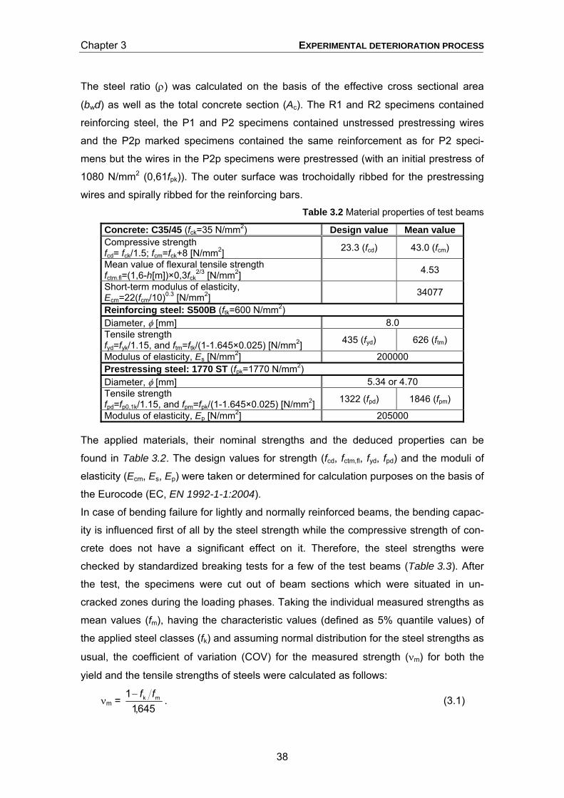
3.3.1.4 Cross-sectional data 41
3.3.2 Test set-up and programme 43
3.3.2.1 Loading phases 44

CONTENTS
3
3.3.2.2 Dynamic measuring phases 48
3.4 SIGNAL PROCESSING 51
3.4.1 Computing individual frequency spectrums 51
3.4.2 Computing average frequency spectrums 53
3.4.3 Computing the average of natural frequencies based on individual
spectrums 56
3.5 RESULTS OF FREQUENCY MEASUREMENTS 58
3.5.1 Natural frequencies for the deterioration states 58
3.5.2 Evaluation technique applied for multiple peaks 60
4 DEFINITION OF DAMAGE INDICES 63 4.1 GENERAL 64
4.1.1 Interpretation of crack-related damage 64
4.1.2 Practical aspects of damage index definition 65
4.1.3 Local versus global indices 65
4.1.4 Cumulative versus incrementative indices 66
4.2 DEFINITION OF DAMAGE INDICES 67
4.2.1 Non-model-based indices 69
4.2.1.1 Growth of total length of cracks 69
4.2.1.2 Growth of total and residual deflection at midspan 70
4.2.1.3 Growth of crack width at midspan 72
4.2.2 Model-based indices 72
4.2.2.1 Growth of “total of crack sections” 75
4.2.2.2 Growth of calculated midspan deflection 75
4.2.2.3 Growth of calculated crack width at midspan 76
4.2.2.4 Growth of internal strain energy 76
4.2.3 Comparison of non-model-based and model-based indices 78
5 DAMAGE ASSESSMENT OF MODEL BEAMS 80 5.1 INTRODUCTION 81
5.1.1 Application of damage indices in experimental damage identification
and assessment 81
5.1.2 Introduction of test results 82
5.2 ANALYTICAL AND NUMERICAL CALCULATIONS 86
5.2.1 Analytical estimations 86
5.2.2 Numerical estimations 87
5.3 DAMAGE IDENTIFICATION OF MODEL BEAMS 89

CONTENTS
4
5.3.1 Detection 89
5.3.2 Quantification 91
5.3.3 Localization 92
5.3.4 Unusual symptoms in frequency trends 92
5.4 DAMAGE ASSESSMENT OF MODEL BEAMS 93
5.4.1 Reinforced (non-prestressed) beams 94
5.4.2. Prestressed beams 98
5.4.3 Post-tensioned beams 105
6 PRACTICAL APPLICATION OF FREQUENCY MEASUREMENTS 109 6.1 GENERAL 110
6.1.1 Aspects for practical application 110
6.1.2 Assumption on the excitation effect caused by road traffic 111
6.2 INTRODUCTION OF THE IN-SITU TEST 111
6.2.1 The investigated structure 111
6.2.2 Excitation of the structure 112
6.2.3 Statistic-based signal evaluation 113
6.2.4 Identification of mode shapes 115
7 SUMMARY AND NEW SCIENTIFIC RESULTS 117 7.1 SUMMARY OF THE THESIS 118
7.2 PRACTICAL APPLICABILITY AND POSSIBLE FURTHER DEVELOPMENT
OF THE RESEARCH 119
7.3 ACKNOWLEDGEMENT 119
7.4 LIST OF THE NEW SCIENTIFIC RESULTS 120
REFERENCES 124 Publications referred in the main text of the dissertation 125
Publications referred in the new scientific results 133
APPENDIX A1 ASPECTS OF CONDITION CONTROL FOR CIVIL ENGINEERING
STRUCTURES A1
A1.1 Inspection versus monitoring A1
A1.2 Diagnostic techniques A3
A1.2.1 Local diagnostic techniques A3
A1.2.2 Global diagnostic techniques (methods) A5
A1.3 Damage assessment for civil engineering structures A6
A1.3.1 Linear versus nonlinear damage assessment A6

CONTENTS
5
A1.3.2 Damage (condition) indices A9
A1.3.3 Environmental effects A12
A2 EXCITATION TECHNIQUES IN VIBRATION-BASED CONDITION
CONTROL A13
A2.1 Ambient excitation A14
A2.2 Excitation by mechanical forces A15
A3 LITERATURE REVIEW OF VIBRATION-BASED DAMAGE IDENTIFICATION
METHODS A16
A3.1 Damage identification based on changes in the basic modal
parameters A16
A3.1.1 Methods based on changes in the natural frequencies A16
A3.1.2 Methods based on changes in the mode shapes and in their
derivatives A24
A3.1.3 Methods based on changes in damping parameters A30
A3.2 Damage identification methods based on dynamically measured
flexibility A31
A3.2.1 Differentiation of methods A31
A3.3 Matrix update methods A32
A3.3.1 Mathematical background A32
A3.3.2 Differentiation of methods A33
A3.4 Nonlinear damage identification methods A34

NOTATIONS
6
GENERAL NOTATIONS
M mass matrix of the structure
K, D stiffness matrix of the structure
G flexibility matrix of the structure
C damping matrix of the structure
Φ mode shape matrix
kN stiffness matrix of N-th element of the structure
εN deformation matrix of N-th element of the structure
{F} load vector
{u} displacement vector
φ mode shape vector
ω, λ, f natural frequency
a acceleration or deflection
w crack width
W internal strain energy
t time
ρ curvature
ε specific strain
M bending moment
A area

1 INTRODUCTION

Chapter 1 INTRODUCTION
8
1.1 GENERAL Civil engineering (CE) structures are built to fulfil one or more functional demand set by
the owners on the basis of service obligations, private reasons or business considera-
tions. The design of a civil engineering structure is determined by:
technical,
economic and
aesthetic
requirements. Normally, the technical requirements are given by standards and other
technical specifications. The appearance of the whole structure, the type of the load
bearing structure and the applied materials (concrete, steel, timber, masonry, etc.) are
chosen by the designers taking into account the above requirements. In many cases
the structure which will be realized is selected in a design competition.
1.1.1 Design working life CE structures are intended to fulfil their functional demands for a given period of time
(design working life). According to experience, the structures can be kept in service
economically at the intended technical level with the specified structural reliability (i.e.
safety and serviceability) during this period. The envisaged design working life accord-
ing to the Eurocode (EN 1990, 2002) for CE structures with different functions can be
seen in Table 1.1. Table 1.1 Design working lives according to the Eurocode (EN 1990, 2002)
Indicative design working life [in years] Examples
10 Temporary structures 10 to 25 Replaceable structural parts 15 to 30 Agricultural and similar structures
50 Building structures and other common structures 100 Monumental building structures, bridges
1.1.2 Deteriorating effects During their working life, CE structures are exposed to various deteriorating effects that
unfavourably influence their durability.
Under usual service conditions the expected service loads cause ageing of both the
whole structure and the component materials. If these loads have a cyclic character
then fatigue-type damage may occur depending on the sensitivity of the structure to
fatigue.
Chapter 1 INTRODUCTION
9
Accidental actions due to human activities (e.g. collisions) or natural disasters (e.g.
earthquakes), excluding the cases when their severity are too high and, due to this, the
structure collapses, generally cause local damage to the load bearing structure. This
local damage may lead to a local functional disorder, which - depending mainly on duc-
tility and the structural type - may be the basis for damage, which gradually develops
due to the effects of the normal service loads.
Aggressive environmental effects cause corrosion on the exposed parts of the structure
which may result degradation in the material properties or - in more severe stages -
directly influence the reliability of the structure. Depending on the aggressiveness of
the environmental conditions, the Eurocode (EN 206-1, 2000; EN 1992-1-1, 2004) de-
fines different exposure classes for concrete structures. For structures in each class,
different values of parameters connected with the durability and different serviceability
requirements have to be taken into account in the design. Nowadays, considerable
number of papers and research projects (COST, 2003) deal with the influences of un-
favourable ambient conditions on the durability of CE structures, especially for
prestressed concrete structures (Mutsuyoshi et al., 2004).
According to the experience on concrete structures, the environmental attacks have a
more significant effect on the durability than the usual service loads and the accidental
actions. This relates especially to concrete highway bridges built in continental regions
and exposed to frequently applied de-icing materials to maintain the function of the
bridge in wintertime degrade the durability of reinforced concrete very quickly
(Andrade, 2003).
1.1.3 Maintenance of CE structures After a certain period of time in service and without any preventive measures and ac-
tivities against the above deteriorating effects, the structural reliability of a structure
may drop below an acceptable level set by the relevant standards. At that time the ex-
isting durability deficiencies may turn into a structural problem. It means that from this
time the necessary design requirements are no longer entirely fulfilled. To raise the
reliability above the acceptable level again, generally the application of a cost-sensitive
rehabilitation, repair or strengthening procedure is needed.
1.1.3.1. Life-cycle cost analyses A maintenance system is intended to keep the reliability (safety and serviceability) of
structures between the designed and the acceptable technical level consuming the
minimum possible costs throughout the full working life. This cost minimization can only

Chapter 1 INTRODUCTION
10
be achieved by the application of an effective resource management system that fo-
cuses straight on the life-cycle cost.
The life-cycle cost (i.e. total cost in Fig. 1.1) of a CE structure includes not only the con-
struction cost invested during the construction period but all the other costs (such as
maintenance cost, operating cost, cost of loss due to unserviceability, cost of loss due
to local failures, etc.) arising during the usual service of the structure. Parts of the latter
group of costs can be taken as approximately constant every year (foreseeable main-
tenance and operating costs) but the others highly depend on the applied risk, which
can numerically be transformed into reliability of the structure (Fig. 1.1). Within the life-
cycle cost management, all the above costs incurred during a given reference period,
which is generally equal to the design working life, are summarized to get the total cost
function of the structure. The minimum of this function in the cost-reliability diagram
according to Fig. 1.1 gives the optimal reliability, which the design of the structure
should be based on.
Fig. 1.1 Costs of a CE structure
This indicates that:
• how crucial the life-cycle cost analysis is when managing highly important and
expensive CE structures in long term, and
• the applied maintenance system should be in accordance with that assumed in
the life-cycle cost analysis (see Sect. 1.2).
This life-cycle cost analysis has been successfully applied to road design in the USA to
compare alternative concrete pavement designs (Waalkes, 2003). This was clearly
used as an economic tool that determined which alternative had the best value. This
analysis is much more difficult for complex CE structures due to the considerably
higher number of variables that influence the performance of the structure compared to
Reliability
Cos
ts
Optimum reliability
Construction costs
Constant annual maintenance and operating costs
Risk-dependent maintenance and operating costs
Total cost

Chapter 1 INTRODUCTION
11
that for pavements but an appropriately simplified, life-cycle cost analysing procedure
should be an achievable goal for bridge managing companies in the near future as
well.
1.1.3.2 Maintenance program and need for condition control Following that a previous (possibly life-cycle cost) analysis declared the necessary ex-
tent of maintenance in the life-cycle resource management system, a maintenance
program has to be elaborated, which contains the necessary maintenance strategies,
measures, tools and activities to be applied in practice.
The amount of cost to be spent annually during the maintenance of a CE structure
(constant annual maintenance cost) mainly depends on the age and – in close relation
to this - on the general condition (information on the degree and severity of deteriora-
tion-induced damage, the current level of reliability compared to the acceptable level,
etc.) of the structure. In order to be able to rationally plan a maintenance program and,
as part of this, to minimize the maintenance cost for the future a database is needed
which contains up-to-date information on the general condition of structures to be kept
in service.
For this reason, in 1998, the Hungarian concrete highway bridges were classified into
the following five categories depending on their level of deterioration (Farkas, 1998)
(Fig. 1.2). The classification was based solely on visual inspections.
Class 1: No visible deterioration, good general condition
Class 2: Initial deterioration (small, local damage only)
Class 3: Medium deterioration
Class 4: Considerable deterioration (insufficient reliability caused by advanced
corrosion)
Class 5: Dangerous condition (structural stability problems).
This situation has been favourably changed a bit after the large extension of the na-
tional motorway network in the last few years. Since 2003 the number of motorway and
highway bridges operated by the State Motorway Management Co. and the Hungarian
Roads Management Co. increased by approximately 10% (Bedics et al., 2008). Yet,
the proportion of bridges belonging to Classes 2-5 is higher than 50% in 2010. The
structural reliability of these bridges is lower than required, therefore in these cases
effective rehabilitation is expected in the near future.

Chapter 1 INTRODUCTION
12
24,2
47,0
24,0
4,60,3
0
10
20
30
40
50
60
1 2 3 4 5Condition classes
[%]
Fig. 1.2 Distribution of the Hungarian concrete highway bridges amongst the condition classes
(from Farkas, 1998)
A similar program is running in the USA (Chase and Laman, 2000). The Federal High-
way Administration (FHA) controls 473,594 highway bridges on the territory of the USA,
of which 99,912 (21%) bridges belong to the National Highway System (NHS) which
carries about 60% of all traffic and about 80% of all truck traffic. In 2000, the FHA car-
ried out a thorough survey of all the highway bridges based mainly on visual inspec-
tions. According to the results, 24% of bridges outside the NHS and 28% of bridges on
the NHS were structurally deficient. There were five possible reasons for a bridge to be
classified as structurally deficient (in the sequence of occurrence regarding the total
number of bridges):
• structural evaluation rating of 2 or less (in a 5 grade scale, 5 is the best value)
• bad substructure
• bad deck
• bad superstructure
• waterway appraisal rating of 2 or less (in a 5 grade scale, 5 is the best value).
For structurally deficient bridges on the NHS, the most frequently found reasons were:
bad deck and bad substructure. Although only 6% of structurally deficient bridges be-
long to the NHS, 43% of the structurally deficient deck area (over 88% of them are
made of concrete) is on the NHS. As a final solution to reduce the number of structur-
ally deficient bridges, currently the USA replaces these bridges at a rate of about 5,600
per year but the strategic goal established by the FHA is 7,000 per year.
According to the current situation and its extrapolation into the near future in Japan
(Fig. 1.3), the number of highway bridges older than 50 years will reach half of all high-
way bridges by 2030.
Chapter 1 INTRODUCTION
13
Fig. 1.3 Prognosis for the future in Japan regarding the age of highway bridges
(from Fujino and Abe, 2001)
All the above national bridge condition evaluation programs conclude the need to de-
velop and to apply condition control systems, which are able to record and to evaluate
structural conditions before deterioration results in visible symptoms, and to provide
rapid, reliable and quantitative measurement of bridge performance in practice.
1.2 CONDITION CONTROL OF CIVIL ENGINEERING STRUCTURES Engineers need to know the actual causes and the possible consequences of sudden
damage or continuous deterioration due to long term environmental and aging proc-
esses on the structural reliability of a CE structure in order to make meaningful and
cost-effective management decisions (Enright and Frangpool, 2000). Early detection
and localization of structural defects allows the owners to plan conveniently pro-
grammed repair and renovation works. Therefore a condition control system, which
covers:
official measures
scheduled investigation programs, including
o the type and frequency of inspections/monitoring
o the components of structures to be investigated
o the performance criteria to be fulfilled
o the rules for documentation of the results
measures to be done if performance criteria are not fulfilled
and is able to quickly mobilize condition evaluation procedures, is an essential need for
owners to maintain CE structures in recent days. The recently published fib Model
Code for Service Life Design (fib, 2006) proposed condition control levels according to
Table 1.2 in order to keep the appropriate level of reliability for CE structures during
their service life.

Chapter 1 INTRODUCTION
14
Table 1.2 Condition Control Levels in the fib Model Code for Service Life Design (fib, 2006)
Condition Control Levels Characteristics Examples
CCL3 Extended inspectionSystematic inspection and monitoring of relevant parameters for the deterioration process(es) that is (are) critical
CCL2 Normal inspection Regular visual inspection by qualified personnel CCL1 Normal inspection No systematic monitoring nor inspection
CCL0 No inspection No possible inspection, for instance due to lack of access
Sect. A1 summarizes the main aspects of the existing condition control systems ap-
plied to CE structures then provides background to their comparison.
Condition control systems are mainly intended to identify damage. A full damage identi-
fication procedure consists of four levels; all levels include the previous level, as follows
(Rytter, 1993; Doebling et al., 1996):
Level 1: Detection: Determination that damage is present somewhere in the
structure
Level 2: Localization: Determination of the geometric location of the damage in
the structure
Level 3: Quantification of the severity of the damage
Level 4: Prediction of the remaining service life of the structure.
To perform Level 1, suitable diagnostic techniques (see Sect. A1.2) are needed as a
minimum. To perform Level 2 and especially Level 3, in addition to suitable diagnostic
techniques, the key issue is the experience of the working staff.
At this point, a clear distinction has to be made between the concepts of “damage iden-
tification” and “damage assessment”. In this context, damage assessment means an
evaluation process (method), which provides information on the structural performance
of a CE structure based on the analysis of the global response data. Therefore, dam-
age identification should be considered as a precondition for damage assessment be-
cause it covers activities, which focus mainly on the first three of the above levels
(Level 1-3).
Using these definitions it becomes obvious that the realisation of Level 4 is only possi-
ble if a damage assessment of the structure is made first in order to obtain information
on the current performance of the structure. Then, in the possession of the structural
performance data, the evaluation of the long-term behaviour (service life prediction) of
the damaged structure can be performed on a reliability basis and, if necessary, by
fatigue life analysis.

Chapter 1 INTRODUCTION
15
Consequently, the above levels of a full damage identification procedure should be
extended by a new intermediate level, which is a precondition to perform Level 4 and
called Level 3a, which aims to provide information on the performance of the whole
structure by using a damage assessment method as follows:
Level 3a: Evaluation of the structural performance based on damage assess-
ment.
In this thesis, mainly the proposed Level 3a will be addressed. Sect. A1.3 discusses
the important aspects of damage assessment.
1.3 VIBRATION-BASED DAMAGE IDENTIFICATION AND ASSESS-MENT FOR CE STRUCTURES - AN OVERVIEW This section gives an overview and deals only with general considerations, while the
state-of-the-art of the vibration-based damage identification methods based on a de-
tailed literature review can be found in Sect. 1.4.
1.3.1. History The engine of the development of vibration-based damage identification methods in
civil engineering fields were, as usual in any technical area, spectacular failures result-
ing in loss of human lives (catastrophes), economic concerns (cost-effective mainte-
nance) and technical innovations (computer-based measuring and evaluating tools).
The idea of dynamic-based damage identification for special CE structures arose when
the oil industry started to pay considerable attention to the assessment of offshore
structures (oil platforms and light stations). The first achievements were introduced at
the Offshore Technology Conferences held in the USA in the 1970s. Later, from the
early 1980s, these techniques and methods have been applied to aerospace structures
(space shuttles and robots). Thanks to the promising first results achieved in this field
and the catastrophic bridge collapses (Tacoma Narrows Bridge, 1940, Silver Bridge at
Point Pleasant, 1967), the application of these methods for bridges considerably in-
creased from the 1980s. Nowadays vibration-based damage identification is mainly
used as part of a monitoring program for bridges. Additionally, vibration-based damage
identification has also been applied to many types of CE structures such as simple
steel, concrete, composite elements of prefabricated structures as well as frames, en-
tire buildings, dams, tanks, vessels, pipes, etc. (Doebling et al., 1996, 1998). It is also
frequently used for experimental purposes.

Chapter 1 INTRODUCTION
16
1.3.2 Vibration-based damage identification methods The basic idea of these methods is that modal characteristics (natural frequencies,
mode shapes, modal damping) are functions of the physical (mass, stiffness, internal
damping) as well as structural (geometry, support conditions) properties of the struc-
ture. Therefore any change in the physical and/or structural properties induces a
change in the modal characteristics, which can be detected by suitable diagnostic
techniques.
The vibration-based damage identification methods can be classified by different as-
pects as follows:
a) Damage identification level
As introduced in Sect. 1.2, Level 1,2,3 and the proposed Level 3a are the central fields
of damage identification for CE structures. However, it is impossible to define exact
limits between these levels and to list methods that concentrate on only one of them.
Methods dealing with damage identification generally address more of the above levels
but their applicability and efficiency on each level is different. Therefore, the governing
rule of the categorization of damage identification methods given in Sect. 1.4 is not the
level which is addressed, but the dynamic characteristic which is measured and/or ana-
lysed.
b) Linear versus non-linear methods
In Sect. 1.4, first of all linear damage identification methods (see Sect. A1.3.1) which
focuses on deducing change in the mechanical and the structural properties of a struc-
ture from the change in its modal properties will be discussed. Non-linear methods
identifying and assessing non-linear structural response and non-parametric models
will only be summarized in Sect. 1.4.4 and Sect.A3.4.
c) Model-based versus non-model-based methods
The damage assessment procedure may be either model-based or non-model-based.
Model-based methods are supplemented by previously adjusted, robust numerical
models and the identification is based on the comparison between the numerically cal-
culated and the measured modal quantity. The practical applicability of these model-
based methods is limited because previous tests are needed to properly adjust the
numerical model and considerable amount of time-consuming numerical computation
has to be carried out. Since either the available finite element (FE) softwares are only
capable of linear-elastic processing or the use of their built-up non-linear modules is
time-consuming, the FE supported model-based methods are generally linear methods.

Chapter 1 INTRODUCTION
17
The non-model-based methods are fully based on modal data measured on-site and
their comparison. For comparative purposes, numerical damage indices (such as MAC,
COMAC, GI, LI, etc., see in Sect. 1.4) are often defined. This is favourable from a prac-
tical point of view, but the efforts made on on-site measurements and signal processing
as well as on the extraction of the necessary modal parameters may also be signifi-
cant. In order to be able to follow the changes in the measured modal data during the
full service life of the structure, a baseline is needed for the comparison. This is gener-
ally the undamaged structure or, if it is not available, the results of a previous meas-
urement. Due to their character, the non-model-based methods are capable of handling
non-linear problems and are often referred to as experimental modal analysis.
1.3.3. Benefits and challenges From the beginning, the practical reasons for the wide and rapid spread of vibration-
based damage identification in the civil engineering fields were as follows:
Information content. The dynamic response of a structure contains all informa-
tion on the structure. If it is fully registered and a global assessment is made,
the location of damage does not need to be known in advance.
Possibility for structural monitoring. The dynamic characteristics are the func-
tions of the physical properties (geometry, mass, stiffness, material law, bound-
ary conditions). If one or more of them change due to, for instance, a possible
damage, it results in a change in the dynamic characteristics. The reversing of
the procedure makes the monitoring of structures theoretically possible.
Practical applicability. The applicability of many diagnostic techniques is limited
due to accessibility and because the installation of the measuring equipment is
difficult (see Sect. A1.2). The dynamic response of a structure can be recorded
at customized (but not optional) points, which allow the positions of the measur-
ing sensors to be chosen to suit the test situation (to maximize the sum of the
magnitudes of the mode shape vectors).
However, the big challenge, which has continuously existed from the beginning, was
the sensitivity of dynamic characteristics to the following effects. These apply to all vi-
bration-based methods which use global damage assessment.
Sensitivity to local damage. Especially the lower modes, which can be meas-
ured easily in-situ, proved to be insensitive to local damage. To develop effec-
tive assessment methods and to define sensitive damage indices, sometimes
complicated algorithms and postprocessing procedures have to be conducted.

Chapter 1 INTRODUCTION
18
Sensitivity to errors. Random errors may be sourced from inevitable noises in
the recorded structural response (environmental effects, electrical disturbances,
background vibration noises, imperfections in the data acquisition system, etc.).
Signal processing errors come from the applied calculation algorithms.
Alampalli (1997) and Messina et al. (1996) investigated the sensitivity of modal
parameters (natural frequencies, modal damping ratios and mode shapes) to
these errors by statistical analysis and found that especially the natural fre-
quencies associated with lower modes were much less sensitive (the maximum
coefficient of variation was smaller than 1%) than other modal parameters.
Similar results have been obtained by Farrar et al. (1997) and Doebling et al.
(1997b).
Sensitivity to environmental effects. Often the distinction between the possible
reasons for a change in the damage index, whether it is caused by real damage
or one (or more) of the ambient effects, is difficult.
Another type of sensitivity analysis was undertaken by Ebert (2001) on reinforced con-
crete beams and plates using a non-linear stochastic finite element model. He as-
sumed stochastic material properties spatially distributed in the structure and studied
the influence of randomly occurring local damage (considered by numerically simulated
cracks) on the change in the modal properties.
1.4 VIBRATION-BASED DAMAGE IDENTIFICATION METHODS (STATE-OF-THE-ART) As a governing rule, the following categorization focuses on the dynamic characteristic
which is measured and/or analysed as a damage index. This can be either one or more
of the basic modal parameters (natural frequencies, mode shapes, damping ratios) or
their derivatives such as mode shape curvatures, strain energy, flexibility, etc. This
review makes a distinction between the model-based and the non-model-based meth-
ods.
The state-of-the-art is mainly based on previous literature reviews of this field by Doe-
bling et al. (1996, 1998), Salawu (1997a), Sohn et al. (2004) and Wenzel et. al (2003).
In this section, only the essence of methods and the conclusions of a deep literature
review on vibration-based damage identification are provided. The full review can be
found in Sect. A3.
Chapter 1 INTRODUCTION
19
1.4.1 Damage identification based on changes in the basic modal parameters In this section, methods which use natural frequencies, mode shapes and damping
ratios as damage indicators are introduced and summarized.
1.4.1.1 Methods based on changes in the natural frequencies In literature, the terms natural frequency, modal frequency and resonant frequency are
often used. However, all three refer to the same item. The applied methods can be
classified as model-based or non-model-based methods.
1.4.1.1.1 Model-based methods
Doebling et al. (1996, 1998) categorized the essences of these methods as solutions
for the forward or the inverse problem.
The forward problem
The methods representing the forward problem generally compare numerically calcu-
lated natural frequencies associated with modelled damage to the corresponding
measured natural frequencies. These methods often lead to iterative procedures and
are usually used for damage detection (Level 1) and sometimes for approximate dam-
age localization (Level 2).
The inverse problem
The inverse problem addresses Level 2 and partly Level 3. These methods calculate
the damage parameters (mainly the damage location and sometimes its severity) from
the measured natural frequency shifts by using so called “prediction” functions describ-
ing how local damage influence the natural frequencies (or their shifts) of the whole
structure. The essence of the difference between the methods solving the forward and
the inverse problem is the application of these prediction functions by the latter meth-
ods.
1.4.1.1.2 Non-model-based methods
Some authors investigated the influence of structural damage on the natural frequen-
cies only experimentally and tried to establish quantitative relationships between the
severity of damage and the change in the natural frequencies.
1.4.1.2 Methods based on changes in the mode shapes and in their derivatives Mode shapes are generally measured to provide spatial information on the dynamic
behaviour of the structure, therefore most often they are used together with natural
frequency measurements. Their parallel use allows more effective damage localization
(Level 2) compared to methods based only on natural frequency measurements.

Chapter 1 INTRODUCTION
20
One part of the methods which analyse mode shape changes use direct displacement
amplitude measurements (displacement mode shapes) while others focus on one or
more derivatives of the mode shapes (slope, curvature, strain energy), which are either
indirectly calculated from the measured displacement mode shapes or directly (experi-
mentally) determined from e.g. strain measurements.
1.4.1.2.1 Methods using displacement mode shapes
These methods can also be categorized as model-based and non-model based meth-
ods.
Model-based methods
Model-based methods investigate the effects of simulated damage on an analytical or a
numerical model. The damage identification (detection, localization and sometimes
quantification) is based on the comparison of the derived model parameters (e.g. am-
plitudes, slopes) with the corresponding measured values.
Non-model-based methods
The non-model-based methods are generally based on modal data correlation by fo-
cusing on the graphical or numerical, direct comparison of the corresponding mode
shapes, which have been experimentally measured in different deterioration states of
the investigated structure (one of them is often the undamaged state used as a base-
line).
The most commonly applied procedures to compare two sets of vibration mode shapes
are the calculation of the Modal Assurance Criterion (MAC) and the Coordinate Modal
Assurance Criterion (COMAC). MAC and COMAC are widely used as global damage
indicators (damage indices).
Naturally, MAC and COMAC values are able to compare any set of mode shape data
such as measured/measured, calculated/measured or calculated/calculated. However,
the biggest advantage of MAC and COMAC is their effective applicability as a non-
model based damage indicator to measured/measured data sets without any prior ana-
lytical or numerical baseline model. Many authors applied MAC and COMAC to com-
pare corresponding mode shapes measured before and after an assumed (in real
situations) or an artificially produced (under laboratory conditions) damage event.
1.4.1.2.2 Methods based on mode shape curvature
For realistic damage in CE structures subjected mainly to flexure, the mode shape dis-
placements change in a very small degree compared to the initial, undamaged state
which makes the application of methods based simply on displacement mode shape
measurements difficult. To improve their sensitivity to damage, a derivative such as the
Chapter 1 INTRODUCTION
21
curvature of a mode shape (mode shape curvature) may alternatively be used instead
of displacement mode shapes for structures subjected mainly to flexure. The expected
improved sensitivity and the ability of these methods for more refined damage identifi-
cation is based on the following assumptions:
• The damage in a structure under bending (M) is tightly accompanied by the reduc-
tion in the bending stiffness (EI), which is in direct relation to the curvature
(M = ρEI). The curvature can be deduced from displacement mode shapes or di-
rectly measured on the structure (Level 1).
• Under constant bending moment, the curvature of a cross-section is fully deter-
mined by the bending stiffness of this cross section (ρ=M/(EI)) but there is no direct
relationship between the curvature and the displacement of the same cross section.
Therefore the curvature is suitable for damage localization (Level 2).
• The size of damage is related to the magnitude of reduction in the bending stiffness
which gives the possibility for approximate damage quantification (Level 3).
The curvature (ρ) at each point of the mode shape can be either calculated by an ap-
propriate formula from the displacement mode shape or directly determined from strain
measurements using the following relationship between strain and curvature for beams
under flexure:
ε = ρ y (1.1)
where ε is the directly measured strain (mostly on the surface of the structure) and y is
the distance between the strain measurement point and the neutral axis.
1.4.1.2.3 Methods based on strain energy
These methods are very similar to, and so, can be considered as an improvement of
methods using mode shape curvatures. The main difference is the quantity which the
applied damage index is based on. For this purpose, the strain energy defined on the
basis of the curvature of the investigated mode shape is applied by these methods.
1.4.1.3 Methods based on changes in damping parameters The most commonly observed damping behaviour of vibrating civil engineering struc-
tures mainly originates from the internal friction of structural materials, which results in
continuous energy dissipation during the motion of the structure. This energy dissipa-
tion is even more intensive in the presence of cracks that open and close during vibra-
tion. This either consumes the input energy given by the exciting effect for structures
under forced vibration or gradually decreases the amplitudes of the free-vibrating struc-
tures. In experimental works, the degree of damping is generally measured by the mo-

Chapter 1 INTRODUCTION
22
dal damping ratio or by the logarithmic decrement of damping. In literature, the damp-
ing models are not exactly elaborated at this stage and, due to this, many modelling
issues are unanswered and many results are contradictory. Notwithstanding, significant
attempts have been made to use the damping characteristics, mainly as an addition to
other damage indices, for damage assessment purposes of civil engineering structures
(Stubbs and Osegueda, 1990a, 1990b; Brincker et al., 1995b).
1.4.2 Damage identification methods based on dynamically meas-ured flexibility Flexibility-based damage identification methods use the flexibility matrix for the charac-
terization of the changes in the structural behaviour. The flexibility matrix [G] defined as
the inverse of the stiffness matrix relates the applied static force {F} to the resulting
displacement {u} of the structure as follows:
{u} = [G] {F} (1.2)
It means that the i-th column of the flexibility matrix represents the displacement pat-
tern of the structure subjected to a unit force applied at the i-th of the degrees of free-
dom (DOF). Hence, the flexibility matrix can be estimated from a modal test using only
on-site data such as the mass-normalized, measured mode shapes {φ}i and the asso-
ciated natural frequencies λi as follows:
[G] = [Φ] [Λ]-1 [Φ]T = Tii
1i 2i
}{}{1
φφλ
∑=
n (1.3)
where [Φ] is the mode shape matrix, [Λ] = diag(λi2) is a diagonal matrix containing the
natural frequency squares and n is the total number of DOF. Although the in-situ
measured mode shapes are not scaled, there are postprocessing techniques to unit
mass-normalize them ([Φ]T [M] [Φ] = [I], where [M] and [I] are the mass and the unity
matrices, respectively) computationally.
For practical applications, damage is generally identified by the comparison of flexibility
matrices synthesized from mode shapes measured on the damaged structure with that
either measured on the undamaged (or a previous baseline) structure or calculated
from a FE model. The synthesis of the complete flexibility matrix from on-site measured
mode shapes is unrealistic due to the fact that only the first few (lowest-frequency)
modes are measured, hence, the [G] matrix computed according to Eq. (1.3) remains
only an estimation. However, because of the inverse relationship to the square of natu-
ral frequencies, the flexibility matrix is most sensitive to changes in these lowest-
frequency modes, which ensures quick convergence when computing it from a limited
Chapter 1 INTRODUCTION
23
number of (low-frequency) modes. This consequently allows handling the flexibility ma-
trix as a reliable damage index for such non-model-based methods.
1.4.3 Matrix update methods Matrix update methods for damage identification are based on fully numerical, mostly
finite element (FE) models. The damaged state of a structure is determined by modify-
ing (updating) the typical structural properties, such as stiffness, mass, and/or damping
properties (matrices), in the FE model to minimize the differences in the modal behav-
iour between the FE model and the damaged structure. If these methods are used for
damage identification, the process starts from the FE model of the undamaged (or pre-
viously damaged and appropriately identified) structure, which perfectly fits its modal
behaviour. Then, its update has to be based on the measured modal data of the dam-
aged structure. The presence, the location and the severity of damage are indicated by
the place and the magnitude of changes made in the FE model parameters during the
update process.
1.4.3.1. Mathematical background The update process mathematically is an optimization problem of the structural equa-
tion of motion: starting from the nominal FE model of the undamaged structure and
iteratively transforming it into the FE model of the damaged structure represented by
the measured modal data.
1.4.3.2. Differentiation of methods The elaborated matrix update methods differ in the mathematical procedures. The op-
timal matrix update methods, the sensitivity-based update methods, the eigenstructure
assignment methods and hybrid methods were applied for identification purposes.
1.4.4 Non-linear damage identification methods The appearance of the non-linear modal behaviour for civil engineering structures was
attempted to be identified in structures with opening and closing cracks. The presence
of such cracks is typical and expected for operating concrete structures but generally
unwelcome and may be the result of local damage for structures made of steel and
other usual materials. The reasons for non-linearities are detailed in Sect. A1.3.1.
Two main issues are analysed in literature. The first is the intensity of the modal test.
Many authors observed that the best way to identify non-linearities in a structure is to

Chapter 1 INTRODUCTION
24
carry out modal tests in different response levels and to evaluate the responses appro-
priately.
The second issue is the applied evaluation procedure with the main focus on the sig-
nal-processing technique. Many techniques are investigated and their sensitivity on
different non-linearities is pointed out.
1.4.5 Conclusions Regarding the considerations listed in Sect. 1.3.3, the achievements of vibration-based
damage identification methods published in literature can be concluded as follows:
A) Information content [A1] Methods based on changes in the basic modal parameters
a) Despite their global nature, the natural frequencies themselves do not provide ex-
act spatial information about local damage with the exception of high natural fre-
quencies, which are associated with local, damage-induced responses.
b) If extending the natural frequency measurements by parallel mode shape re-
cording, theoretically the full spatial information about local damage can be gained.
The higher the number of recorded modes the more complete the information con-
tent of the dynamic response of the structure is.
[A2] Methods based on dynamically measured flexibility, matrix update methods, non-
linear methods
Each of these methods uses the on-site measured natural frequency and associ-
ated mode shape data as input parameters, therefore, the information content of
these methods and their improvement is consequently the same as for methods re-
ferred to above in [A1]/b).
B) Practical applicability [B1] Methods based on changes in the basic modal parameters
a) The lower natural frequencies can be measured with high confidence (with low co-
efficient of variation), therefore they are best suited for field tests. The use of estab-
lished relationships between damage location and natural frequency shifts theoreti-
cally allows limited damage localization in easy circumstances (Level 1 and limited
Level 2).
b) The technical difficulties in installing measurement points and/or the narrow fre-
quency range of the applied excitation often limit the possibility for measuring a
“sufficient” number of high modes (natural frequencies together with associated
mode shapes). For limited number of measured modes, and especially in the ab-

Chapter 1 INTRODUCTION
25
sence of high modes, the limited information content generally does not allow exact
damage localization and quantification even in the possession of measured mode
shapes.
c) The model-based methods require analytically or numerically computed sensitivity
values obtained from an appropriately adjusted model. The considerable amount of
computation needed to model all possible damage events may be performed for
simple laboratory tests but is unrealistic for real structures. Moreover, the accuracy
of these methods highly depends on the quality of the numerical model. Therefore,
the practical applicability of these methods is highly limited. This applies to methods
focusing simply on natural frequency shifts as well as to those analysing natural
frequency and associated mode shape changes simultaneously.
However, some non-model-based methods do not require analytical or numerical
models but use only test data from the measured modes and are based on simple
assumptions about the structural behaviour. This is favourable from a practical
point of view but the effort made on the on-site measurements and the on-site-
recorded signal processing as well as on the extraction of the necessary modal pa-
rameters may also be significant. For these methods a baseline is needed for the
comparison-based evaluation of results, which can be either the undamaged struc-
ture or the results of a previous investigation. The defined numerical damage indi-
ces (MAC, COMAC, GI, LI and MSECR) proved to be efficient in practical cases
and made possible damage localization (Level 2).
d) The damping models are not exactly elaborated at the present stage and, due to
this, many modelling issues are unanswered and many results are contradictory,
therefore, these models are not commonly used in practice.
[B2] Methods based on dynamically measured flexibility, matrix update methods, non-
linear methods
The flexibility methods can be taken as fully non-model-based methods and are
practical for intermittently conducted routine surveys on structures without any
known, present damage and with an appropriately documented previous stage as a
baseline, because quick convergence can be reached when compiling the flexibility
matrix from on-site measured low-frequency modes.
The matrix update methods answer the forward problem (Sect. 1.4.1.1.1) by using
a robust mathematical background (matrix iteration), therefore, they require consid-
erable computational capacity, which greatly limits their practical applicability.

Chapter 1 INTRODUCTION
26
The non-linear methods use similar mathematical means as the matrix update
methods, therefore their applicability in practice is also limited.
C) Sensitivity [C1] Methods based on changes in the basic modal parameters
Each mode has different sensitivity to damage because a frequency shift or a mode
shape change depends on the nature, the location and the severity of the damage.
The insensitivity of lower modes is generally due to their global nature. For damage
located in low stress regions (close to nodes) of the considered mode, the associ-
ated frequency shift or mode shape change will also be insensitive. However, due
to the increased information content on the dynamic response, the sensitivity of
methods focusing on simultaneous natural frequency and associated mode shape
measurements is generally higher than that for methods based simply on natural
frequency measurements.
[C2] Methods based on dynamically measured flexibility, matrix update methods, non-
linear methods
Because of the inverse relationship to the square of natural frequencies, the flexibil-
ity matrix, which is directly used by the flexibility methods, is most sensitive to
changes in these lowest-frequency modes.
In addition to the amount and the quality of input data, which is tightly determined
by the number and the accuracy of measured modes of the investigated structure,
the sensitivity of matrix update methods and non-linear methods is highly affected
by the applied mathematical procedure.

2 FOCUS OF THE THESIS

Chapter 2 FOCUS OF THE THESIS
28
2.1 CONCEPTION OF THE RESEARCH The primary motivation of the research covered by this thesis was already addressed in
Sect. 1.2. A literature review of vibration-based damage identification methods
(Sect. A3) pointed out that the existing methods do not really address such issues,
which are particularly important from the owner’s, the maintainer’s and the designer’s
point of view. These issues are related to structural safety/reliability and durability and
are well-founded input for further decisions regarding the necessity of possible struc-
tural strengthening or the estimation of the remaining service life. The implemented
methods focus only on the first three levels of damage identification (detection, local-
ization and maybe quantification) set by Rytter (1993), but Level 4 as well as the re-
lated safety and durability concerns remain untouched. The need for assessment
methods, which are able not only to identify damage by dynamic methods but to pro-
vide information on the structural performance, led to the proposal of Level 3a as a new
interim level after Level 3 in the above damage identification system defined in
Sect. 1.2. The global purpose of this research was to fulfil Level 3a of crack-related
damage assessment and to carry it out on concrete beams under experimental condi-
tions.
Before defining what tasks are necessary to achieve experimental damage identifica-
tion and assessment, some issues, which are closely touched by this research, have to
be clarified.
2.1.1 Differentiation of model-based and non-model-based methods Many of the existing procedures are supplemented by previously adjusted, robust nu-
merical models. Damage identification is often based on the comparison of numerically
calculated and measured values of the investigated modal quantity. The practical ap-
plicability of these “model-based methods” is limited because previous tests are
needed to properly adjust the numerical model (i.e. to eliminate the model uncertain-
ties) and considerable amount of time-consuming numerical computation has to be
carried out.
The “non-model-based methods” are fully based on on-site-measured modal data and
their comparison. This is carried out by defining numerical damage indices (MAC, CO-
MAC, GI and LI, flexibility matrix, etc.) directly on the basis of the measured data. This
is favourable from a practical point of view but the effort made on on-site measure-
ments and on on-site-recorded signal processing as well as on the extraction of the
necessary modal parameters may also be significant. For monitoring purposes (i.e. to

Chapter 2 FOCUS OF THE THESIS
29
follow the changes in the measured modal data during the service life of the structure)
a baseline, which is generally the undamaged structure, or, if it is not available, the
results of a previous measurement is needed for the comparison.
2.1.2 Model uncertainties in testing concrete structures Fig. 2.1 shows the scheme of static and dynamic tests regularly made on concrete
bridges recently. On-site investigations are usually complemented by analytical or nu-
merical analyses. They are fully based on assumptions regarding the load, the geome-
try, the material properties, the material law and the structural behaviour, which result
in model uncertainties. Consequently, the results of these analytical and numerical
models include the effects of model uncertainties.
Fig. 2.1 Scheme of static and dynamic tests for concrete bridges
The outcome of a typical static test is generally a comparison of the calculated (model-
based) and the measured (non-model-based) values of the investigated quantity,
which, due to the often limited accessibility of the structure, is generally a deformation
or a cracking parameter. If the difference does not exceed an acceptable level, which is
intended to consider model uncertainties, the test is declared successful.
Static modelling
Static response • crack parameters • deflections • and their derivatives
Resistance data
ANALYTICAL AND/OR NUMERICAL ANALYSES
(model-based)
No
mov
emen
t du
ring
test
ASSUMPTIONS (load, geometry, mate-rials, structural behav-iour incl. degradation)
Additional structural behaviour model
(considering movement)
MO
DEL
UN
CER
TAIN
TIES
lo
ad, g
eom
etric
al a
nd m
ater
ial m
odel
+
stru
ctur
al b
ehav
iour
mod
el
a2
STA
TIC
TES
T
Add
ition
al b
ehav
iour
m
odel
unc
erta
intie
s
b Mov
emen
t du
ring
test
Dynamic modelling
Dynamic response (modal analysis) • natural frequencies • mode shapes • and their derivativesD
YNA
MIC
TES
T
Dynamic (vibration) test
Dynamic response Signal recording • ∆-t, a-t functions
Signal processing • frequency spectrum • mode shapes • damping • and their derivatives
Excitation
Static (load) test
Static response • crack parameters • deformation • and their derivatives
EXPERIMENTAL OR ON-SITE INVESTIGATIONS
(non-model-based)
a1
Chapter 2 FOCUS OF THE THESIS
30
When carrying out dynamic modelling (i.e. modal analysis), an additional structural
behaviour model, which appropriately characterizes the structure under vibration, and
therefore, is not included in the static model, has to be adopted. Typically for concrete
bridges, this model describes the behaviour of active (opening and closing) cracks un-
der vibration. For long-term investigations, the degradation of structural parameters
due to cyclic effects may also be necessary to consider in the additional structural be-
haviour model. When executing on-site dynamic tests (signal recording + processing)
and trying to compare the calculated (model-based) dynamic parameters with the
measured (non-model-based) ones, the uncertainties in the additional structural behav-
iour model also work against their exact coincidence.
2.1.3 Reducing or eliminating the effects of model uncertainties Due to the above model uncertainties, it proved to be difficult to find a close coinci-
dence between numerically calculated and corresponding on-site measured dynamic
properties for real structures (Rizos et al. (1990), Salawu and Williams (1994), Farrar
and Jauregui (1998), etc.). The effectiveness of such tests can be improved considera-
bly if:
a) the effect of model uncertainties is reduced or eliminated for the model-based
damage identification procedures;
b) non-model-based damage identification procedures are developed and used.
The model uncertainties are fully eliminated if relationships between measured (non-
model-based) static characteristics and measured (non-model-based) dynamic pa-
rameters are quantitatively described (link a1 in Fig. 2.1). The description of relation-
ships between measured (non-model-based) dynamic parameters and calculated
(model-based) static characteristics is helpful in reducing the number, and conse-
quently, the effect of model uncertainties. Calculated static characteristics are obtained
from static models, therefore their applicability has to be verified by comparison to their
corresponding measured (non-model-based) values through conformity checks (link a2
in Fig. 2.1).
2.1.4 Explaining the omission of dynamic models The omission of dynamic models from damage identification was due to the intention to
ignore model uncertainties, which come when modelling the dynamic behaviour of
damaged concrete beams. Sect. A1.3 introduces how difficult it is to take into account
all parameters which influence the dynamic behaviour of a concrete structure in the

Chapter 2 FOCUS OF THE THESIS
31
dynamic model. Sect. A1.3.1 discusses that especially the crack-related behaviour of
concrete beams often leads to non-linearity, thus, such behaviour can only be de-
scribed by non-linear (numerical, FEM) models. The applicability of analytical models in
these cases is practically impossible. Sect. A3 introduces the extent of computational
effort necessary to develop and run non-linear dynamic models. Their adjustment to
the actual structural response is complicated. Sect. 3.4 verifies how difficult it is to read
out the structural behaviour-related effects from the electronically recorded vibration
signals.
2.1.5 Applied method of work to fulfil Level 3a damage assessment Due to reasons given in Sect. 2.1.4, no dynamic model was developed and, conse-
quently, the structural behaviour of test beams was described by static characteristics
calculated from a static model. Referring to Sect. 2.1.3, static-based damage indices
were defined for identification purposes and structural performance-related static char-
acteristics were defined to reflect on the structural performance of the tested speci-
mens. Hence, the establishment of any relationship between the measured dynamic
properties and the structural performance-related characteristics fulfilled Level 3a dam-
age assessment according to Sect. 2.1.
2.2 GOALS OF THE RESEARCH To address Level 3a damage assessment under experimental conditions, the following
were the goals of this research:
a) Modelling crack-related damage under experimental conditions on various
types of concrete beams;
b) Elaborating signal processing tools to process numerically-recorded vibration
data and then to provide a statistical basis for the determined dynamic parame-
ters (here the first two natural frequencies). Development of appropriate fre-
quency evaluation techniques to reflect on different damage cases.
c) Definition of damage indices, which are able to identify crack-related damage
as well as to measure its extent (identification).
d) Establishing relationships between the measured dynamic parameters and the
related structural performance-characterizing properties (assessment).
e) Application of the method (or one of its part) on a real structure.

Chapter 2 FOCUS OF THE THESIS
32
Although the intended research is not material related, the work in this thesis fully fo-
cused on structures made of concrete and does not aim to deal with any other issues
related to other materials.
2.3 DESCRIPTION OF THE RESEARCH Laboratory tests were conducted to thoroughly describe the crack-related degradation
of concrete model beams by structural performance-related parameters as well as by
basic modal data. For basic modal data, the first two natural frequencies were deter-
mined. Crack-related damage of beams was identified by appropriately defined, static-
based damage indices. Some of these indices (non-model-based indices) were based
simply on experimentally registered (directly-measured) parameters (e.g. crack pattern)
and the others (model-based indices) were obtained by calculations. The assessment
of the structural performance of the test beams included the establishment of relation-
ships between the basic modal data and the structural performance-related parame-
ters, their quantitative description and their conclusion. The tests have been carried out
at the Budapest University of Technology and Economics, Dept. of Structural Engineer-
ing. The practical applicability of frequency measurements was verified by a field test
executed on an existing concrete highway bridge.
2.3.1 Test variables Deterioration of concrete beams due to either aging, environmental attack or mechani-
cal effects generally results in cracking. Crack-related damage identification and as-
sessment carried out on such beams for various reasons often focuses on the determi-
nation of the extent of cracking. Cracking is not only a visible sign of deterioration but a
systematic pattern of individual cracks and, consequently, a structural characteristic
tightly influenced by many performance-related structural parameters. For concrete
beams under flexure, the most important of these parameters are the properties of
bond between reinforcement and concrete, the amount of bending reinforcement as
well as the presence, the bond-related behaviour (bonded or unbonded) and the inten-
sity of prestressing.
Therefore, while using cracking to model the deterioration process, the introduced test
was aimed at investigating the influence of the above test variables on the extent of
cracking and, consequently, on the relationship between basic modal data and the
structural performance-related parameters.
Chapter 2 FOCUS OF THE THESIS
33
2.3.2 Focuses of the chapters Chapter 3 focuses on tasks a) and b) of Sect. 2.2 by introducing the conducted labora-
tory tests. Detailed descriptions of test beams, the execution of the artificial deteriora-
tion process, the measured and calculated structural performance-related parameters,
the applied excitation techniques, the dynamic measurements, the signal processing as
well as the procedure of signal evaluation will be given.
Chapter 4 deals with task c) of Sect. 2.2 by defining, determining and classifying static-
based damage indices used for crack-related damage identification purpose.
Chapter 5 focuses on tasks d) of Sect. 2.2 by establishing relationships between the
first two natural frequencies and the structural performance-related parameters for as-
sessment purpose.
Chapter 6 demonstrates the practical applicability of frequency measurements with a
simple dynamic test carried out on an existing concrete highway bridge.
Chapter 7 summarizes the new scientific results of this work.

3 EXPERIMENTAL
DETERIORATION PROCESS

Chapter 3 EXPERIMENTAL DETERIORATION PROCESS
35
3.1 INTRODUCTION
For experimental purposes, simply supported, reinforced, prestressed and post-
tensioned reinforced concrete beams were tested under flexure. No primarily shear-
related behaviour was considered and investigated, therefore all test set-ups were cho-
sen accordingly.
3.2 GENERAL PROCEDURE
All of the test beams first underwent an artificially-produced deterioration process in
several steps. This process was chosen depending on the beam type and, in order to
investigate minor aspects, was slightly modified for a few specimens within the beam
family of the same type. Then for a few of the reinforced (reinforced concrete) beams,
external post-tensioning with gradually increasing intensity as a simulated strengthen-
ing effect was applied in three steps. For the prestressed beams, no post-tensioning
was applied after the deterioration process. In the following, each of the previous dete-
rioration and strengthening steps will be mentioned simply as state and marked by
natural numbers (and by their variations when the general process was slightly modi-
fied) starting from 1 to 5 (7 for P2/1 & P2/2, see Table 3.6) for the deterioration period
and from 6p to 8p (see Table 3.4) for the subsequent strengthening period.
The detailed introduction of the test set-up and the description of the process can be
found in Sect. 3.3.2. The deduction of damage indices on the basis of parameters
characterizing the cracking state of the beam and the computation of modal data from
the registered signals will be detailed in Sect. 3.4.3.
3.2.1 Reinforced concrete (non-prestressed) beams For the reinforced concrete (non-prestressed) beams (R1, R2, P1, P2 in Fig. 3.1) each
state in the deterioration period (from 1 to 5 (7 for P2/1 & P2/2)) included a loading
phase, during which the intended cracking state of the beam was first produced then
the loading was completely removed, and a following measuring phase, during which
dynamic measurements resulting in the investigated modal data were carried out. In
the strengthening period (from 6p to 8p) the system of the applied post-tensioning was
identical; only the intensity of the post-tensioning force increased gradually state by
state but was constant in each state. No removal or decreasing of the post-tensioning
force took place and no external load was applied to the beams between the consecu-
tive states in the strengthening period.

Chapter 3 EXPERIMENTAL DETERIORATION PROCESS
36
3.2.2 Prestressed beams For the prestressed beams (P2p in Fig. 3.1) no strengthening state was applied, fur-
thermore, the loading phases in the deterioration period were significantly modified in
comparison to that for the reinforced concrete beams. Similarly to prestressed beams
used in practice, the cracking and decompression moments of the tested beams were
significantly increased by the applied prestressing therefore very small degree of crack-
ing and consequently very small crack-induced shifts in modal parameters could be
expected at practical load levels (before the design moment capacity is reached). In
fact, the primary deterioration effect for this kind of beam in practice used to be the
breaking of prestressing tendons, which leads to decrease in the prestressing action
and consequently allows more intensive cracking and external load-induced deforma-
tions. For this reason the intended deterioration process for these beams in the test
mainly focused on the investigation of shifts in modal parameters due to gradual ten-
don breaks. For this test, only bonded tendons (in form of wires) were applied, there-
fore the tendon breaks were simulated by simply, mechanically cutting wires through
the concrete cover at many sections along the beam length state by state. After the
prestressing effect had been decreased to some extent, loading phases as part of the
deterioration period and similar to that for the reinforced concrete beams were also
applied.
3.3 DESCRIPTION OF THE TEST
The properties of the test beams, the applied prestressing and post-tensioning system,
the test set-up and the procedure of the test will be detailed.
3.3.1 Test beams The prototypes of the test beams are widely used in practice as precast, prestressed
concrete floor beams in buildings with clear spans ranging between 2.4 m and 6.6 m
(type P2p in Fig. 3.1 can be considered as an original product).
However, in accordance with the aim of the present test, the test beams were manufac-
tured with the same geometry but with different type (reinforcing bar or prestressing
wire) and amount of reinforcement compared to the original product. Other investigated
parameters were the effect of prestressing as well as the application of external post-
tensioning to reinforced concrete (non-prestressed) specimens as a simulation of a
possible strengthening effect.

Chapter 3 EXPERIMENTAL DETERIORATION PROCESS
37
3.3.1.1 Geometric, material and reinforcement properties of the test beams
All the test beams had the same concrete cross section (Fig. 3.1) whose nominal geo-
metric data can be seen in Fig. 3.2.
Fig. 3.1 Cross sections of test beams
The total length was 4.4 m for the R1, R2, P2, P2p marked specimens and 3.4 m for
the P1 marked specimen (Table 3.1). All beams were prismatic, both the concrete sec-
tion and the embedded longitudinal reinforcement were unchanged along the full length
of each beam.
Fig. 3.2 Geometric dimensions of the cross section (notations)
The beams had different types of reinforcement and different steel ratios according to
Fig. 3.1 and Table 3.1. Table 3.1 Geometrical and reinforcement data of test beams
Length Reinforcement Steel ratio, ρ [%] Beam
type No. of beams
Total lengthLb [m]
Span L [m]
Strength fpk/fp0,1k or ftk/fyk
[N/mm2] Type (surf.)
No. & φ [mm] of
bars As/(bwd) As/Ac
Initial prestress
P1 1 3.4 3.2 1770/1520 prestressing steel (tr.) 2φ5.34 0.527 0.284 unstressed
R1 4 4.4 3.8 600/500 reinforcing steel (sp.) 2φ8 1.183 0.636 -
P2 3 4.4 3.8 1770/1520 prestressing steel (tr.)
(7+1) φ4.7 1.436 0.769 unstressed
R2 3 4.4 3.8 600/500 reinforcing steel (sp.) 3φ8 1.774 0.955 -
P2p 3 4.4 3.8 1770/1520 prestressing steel (tr.)
(7+1) (5+1) (3+1) (2+1) φ4.7
1.436 1.040 0.645 0.449
0.769 0.549 0.329 0.220
0.61fpk
R1 R2 P2P1 P2p
kt
kc
a
bc
bt
dbw
hc
hw
ht
h
Nominal sizes [mm] h 190 bc 80 bw 50 hc 60 kc 15 hw 65 kt 5 ht 45 bt 140 a 20
Chapter 3 EXPERIMENTAL DETERIORATION PROCESS
38
The steel ratio (ρ) was calculated on the basis of the effective cross sectional area
(bwd) as well as the total concrete section (Ac). The R1 and R2 specimens contained
reinforcing steel, the P1 and P2 specimens contained unstressed prestressing wires
and the P2p marked specimens contained the same reinforcement as for P2 speci-
mens but the wires in the P2p specimens were prestressed (with an initial prestress of
1080 N/mm2 (0,61fpk)). The outer surface was trochoidally ribbed for the prestressing
wires and spirally ribbed for the reinforcing bars. Table 3.2 Material properties of test beams
Concrete: C35/45 (fck=35 N/mm2) Design value Mean value Compressive strength fcd= fck/1.5; fcm=fck+8 [N/mm2] 23.3 (fcd) 43.0 (fcm)
Mean value of flexural tensile strength fctm.fl=(1,6-h[m])×0,3fck
2/3 [N/mm2] 4.53
Short-term modulus of elasticity, Ecm=22(fcm/10)0.3 [N/mm2] 34077
Reinforcing steel: S500B (ftk=600 N/mm2) Diameter, φ [mm] 8.0 Tensile strength fyd=fyk/1.15, and ftm=ftk/(1-1.645×0.025) [N/mm2] 435 (fyd) 626 (ftm)
Modulus of elasticity, Es [N/mm2] 200000 Prestressing steel: 1770 ST (fpk=1770 N/mm2) Diameter, φ [mm] 5.34 or 4.70 Tensile strength fpd=fp0,1k/1.15, and fpm=fpk/(1-1.645×0.025) [N/mm2] 1322 (fpd) 1846 (fpm)
Modulus of elasticity, Ep [N/mm2] 205000
The applied materials, their nominal strengths and the deduced properties can be
found in Table 3.2. The design values for strength (fcd, fctm,fl, fyd, fpd) and the moduli of
elasticity (Ecm, Es, Ep) were taken or determined for calculation purposes on the basis of
the Eurocode (EC, EN 1992-1-1:2004).
In case of bending failure for lightly and normally reinforced beams, the bending capac-
ity is influenced first of all by the steel strength while the compressive strength of con-
crete does not have a significant effect on it. Therefore, the steel strengths were
checked by standardized breaking tests for a few of the test beams (Table 3.3). After
the test, the specimens were cut out of beam sections which were situated in un-
cracked zones during the loading phases. Taking the individual measured strengths as
mean values (fm), having the characteristic values (defined as 5% quantile values) of
the applied steel classes (fk) and assuming normal distribution for the steel strengths as
usual, the coefficient of variation (COV) for the measured strength (νm) for both the
yield and the tensile strengths of steels were calculated as follows:
νm = 645,1
1 mk ff−. (3.1)

Chapter 3 EXPERIMENTAL DETERIORATION PROCESS
39
Table 3.3 Results of standardized breaking tests of cut-out steel specimens
Reinforcing steel (φ8 mm; S500; fyk=500 N/mm2; ftk=600 N/mm2) Measured
load [kN] strength [N/mm2]Coefficient of varia-
tion (COV) Beam type
Nominal cross-sectional area
[mm2] Fym,m Ftm,m fym,m ftm,m νy,m νt,m R1/1 50.3 29.3 31.6 583 629 0.086 0.028 R2/2 50.3 29.8 31.9 593 635 0.095 0.033 R2/2 50.3 28.8 30.7 573 611 0.077 0.011
average: 0.086 0.024 Prestressing steel (φ4.7 mm; fp0,1k=1520 N/mm2; fpk=1770 mm2)
Measured load [kN] strength [N/mm2]
Coefficient of varia-tion (COV) Beam
type
Nominal cross-sectional area
[mm2] Fp0,1m,m Fpm,m fp0,1m,m fpm,m νp0,1,m νp,m P2/3 17.3 28.0 32.0 1614 1844 0.035 0.025
When determining the mean tensile strength of steels (ftm, fpm) in Table 3.2 for cross-
sectional data calculations, the applied COV values equal to 0.025 were taken on the
basis of the average COV obtained in Table 3.3.
3.3.1.2 Reduction of prestress in the P2p specimens For the prestressed P2p type specimens, the deterioration process was partly modelled
by artificial tendon breaks made by sawing the intended number of wires in the bottom
flanges of the beams through the concrete cover at selected cross-sections (cut points)
along the beam length as shown in Fig. 3.3. The numbers below the cut points show
the number of cut wires at that particular section in the corresponding state.
Fig. 3.3 Wire cuts for the P2p specimens
For the P2p/1 specimen, first gradual wire cuts were made only at two sections sym-
metric to the midspan (states 41-44). Then the cuts were expanded uniformly for the
full span (states 5-55) producing a relatively smooth transition in the prestressing force.
0 - - - - 0 - 2 - - - - 0 - 2 - - - - 2 - 4 - - - - 2 - 4 - - - - 4 - 4 0 0 0 0 4 04 0 0 4 0 4 04 0 2 4 2 4 04 2 2 4 2 4 24 2 4 4 4 4 24
State 3 State 41 State 42 State 43 State 44 State 5 State 51 State 52 State 53 State 54 State 55 4 4 4 4 4 4
8×L/8=3.8 m
P2p/1 P2p/2 & P2p/3
0.4 0.4 0.5 2× 0.25
2× 0.25
0.5 0.5 0.5
L = 3.8 m
0State 2 0 0 0 0 0 0 2State 3 2 2 2 2 2 2 5State 4 5 5 5 5 5 5
025
2 cut wires 4 cut wires 5 cut wires
< 2 mm ~20 mm
cut size

Chapter 3 EXPERIMENTAL DETERIORATION PROCESS
40
For the P2p/2 and P2p/3 specimens, this transition was quicker because five wire cuts
at each cut point were completed through only two states. Note that for the P2p/2 and
P2p/3 specimens the cut points are not uniformly distributed along the span but rather
positioned toward the midspan. In state 3 for the P2p/1 beam and state 2 for the
P2p/2&3 beams, only the concrete cover was sawed without any wire cuts.
Because of full bond around the tendons, individual wire cuts result in only a local de-
crease of the prestressing action along the span. This decrease was considered as
linear along the transmission length (lpt) on both sides of the cut, which was calculated
on the basis of the mean value of tensile strength (fctm) of concrete according to the EC
as follows:
lpt = α1α2φm.bpt
eff,p
fσ
= 165 mm. (3.2)
Here fbpt.m=ηp1η1fctm is the mean value of bond stress and φ is the diameter of indented
wire (ηp1=2,7) with circular cross section (α2=0,25). Sudden stress release (α1=1.25)
and “good” bond conditions (η1=1,0) were assumed. As a result of this, all prestressing
related data suddenly changed at the cut points and were consequently considered as
functions of distance along the beam length as shown in related figures of Sect. 3.3.1.4
and Sect. 3.3.2.1.
3.3.1.3 Details of post-tensioning To simulate a possible strengthening effect, a few, reinforced concrete beams (P1,
R1/4, R2/1, P2/1 and P2/2) were equipped with an external post-tensioning system
after the intended deterioration process (according to Sect. 3.3.2) had been completed.
anchored end active end
Fig. 3.4 Post-tensioning equipment
This system consisted of two unbonded, ST 1860 type, wedge-anchored, nearly centri-
cally-positioned, straight-line monostrands with a cross-section of 150 mm2 each and
40 mm thick anchorage plates at both ends. The tensioning force was applied simulta-

Chapter 3 EXPERIMENTAL DETERIORATION PROCESS
41
neously in both strands in three steps (6p, 7p and 8p according to Table 3.4) by a
608 kN (650 bar) capacity hydraulic jack, whose self-weight was measured as 0.3 kN,
at one end of beams (Fig. 3.4). The tensioning process was monotonic, thus the ten-
sioning force was not removed or decreased between the consecutive tensioning
steps. The general arrangement of the post-tensioning system for the P1 marked
specimen is shown in Fig. 3.5.
Fig. 3.5 Arrangement and geometry of post-tensioning for the P1 specimen
The tensioning force was intentionally centric, but owing to the different reinforcements
slightly varying eccentricity occurred in the vertical plane for the different beam types.
However, considering its extent, the resulting flexural effect was quite low and the cen-
tric compression effect remained dominant. Table 3.4 Post-tensioning force control measurements for the P1 specimen
Respective Measured slips [mm] Calculated (with Ep=195000 N/mm2) force [kN] per anchored
end, ∆1
active end ∆2,1-∆2,2
shortening [mm]
stress [N/mm2] strand beam
Post-tensioning
step
pres-sure in
jack [bar]
force per
strand [kN] one
side other side
one side
other side
one side
other side
one side
other side
one side
other side
ave-rage total
6p 21 10 8.6 8.2 19.0 20.0 taken as zero 67 67 10 10 10 20 7p 203 95 6.5 6.4 31.0 34.0 9.9 12.2 562 677 84 102 93 1868p 321 150 5.8 5.5 39.4 40.3 17.6 17.6 947 947 142 142 142 284
The applied, pressure-adjusted tensioning force was controlled by measuring the
wedge slips at both ends (∆1 and ∆2,2) as well as the push-out length of the jack (∆2,1)
after each stressing step for the P1 marked specimen. Because of the good coinci-
dence between the intended and the deduced force (<5%) no further control was found
to be necessary (Table 3.4). In the following the intended post-tensioning forces (10, 95
and 150 kN/strand for states 6p, 7p and 8p respectively) will be taken into account for
calculation purposes.
3.3.1.4 Cross-sectional data Cross-sectional data of the test beams (Table 3.5) were calculated on one hand as
input for the deduction of damage indices and on the other hand to provide background
information to the applied loading phases.
P
dP S eP≈0
∆1 ∆2.2
∆2.1
100 1003200 3400
dP=120 mm
500
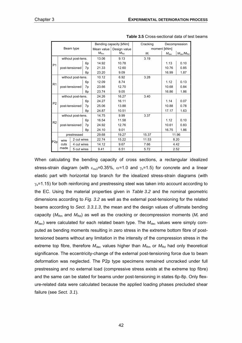
Chapter 3 EXPERIMENTAL DETERIORATION PROCESS
42
Table 3.5 Cross-sectional data of test beams
Bending capacity [kNm] Cracking Decompression moment [kNm] Beam type Mean value
MRm Design value
MRd Mr Mdec Mdec/MRd
without post-tens. 13.06 9.13 3.19 6p 14.92 10.78 1.13 0.10 7p 21.33 12.60 10.76 0.85
P1 post-tensioned
8p 23.20 9.09 16.99 1.87 without post-tens. 10.12 6.92 3.28
6p 12.09 8.74 1.12 0.13 7p 23.66 12.70 10.68 0.84
R1 post-tensioned
8p 23.74 9.05 16.86 1.86 without post-tens. 24.26 16.27 3.40
6p 24.27 16.11 1.14 0.07 7p 25.06 13.88 10.88 0.78
P2 post-tensioned
8p 24.87 10.51 17.17 1.63 without post-tens. 14.75 9.99 3.37
6p 16.54 11.58 1.12 0.10 7p 24.92 12.76 10.61 0.83
R2 post-tensioned
8p 24.10 9.01 16.75 1.86 prestressed 29.68 19.27 15.37 11.96
2 cut wires 22.74 15.22 11.53 8.20 4 cut wires 14.12 9.67 7.66 4.42
P2p wire cuts
made 5 cut wires 9.41 6.51 5.72 2.52
When calculating the bending capacity of cross sections, a rectangular idealized
stress-strain diagram (with εcu3=0.35%, α=1.0 and γc=1.5) for concrete and a linear
elastic part with horizontal top branch for the idealized stress-strain diagrams (with
γs=1.15) for both reinforcing and prestressing steel was taken into account according to
the EC. Using the material properties given in Table 3.2 and the nominal geometric
dimensions according to Fig. 3.2 as well as the external post-tensioning for the related
beams according to Sect. 3.3.1.3, the mean and the design values of ultimate bending
capacity (MRm and MRd) as well as the cracking or decompression moments (Mr and
Mdec) were calculated for each related beam type. The Mdec values were simply com-
puted as bending moments resulting in zero stress in the extreme bottom fibre of post-
tensioned beams without any limitation in the intensity of the compression stress in the
extreme top fibre, therefore Mdec values higher than MRm or MRd had only theoretical
significance. The eccentricity-change of the external post-tensioning force due to beam
deformation was neglected. The P2p type specimens remained uncracked under full
prestressing and no external load (compressive stress exists at the extreme top fibre)
and the same can be stated for beams under post-tensioning in states 6p-8p. Only flex-
ure-related data were calculated because the applied loading phases precluded shear
failure (see Sect. 3.1).
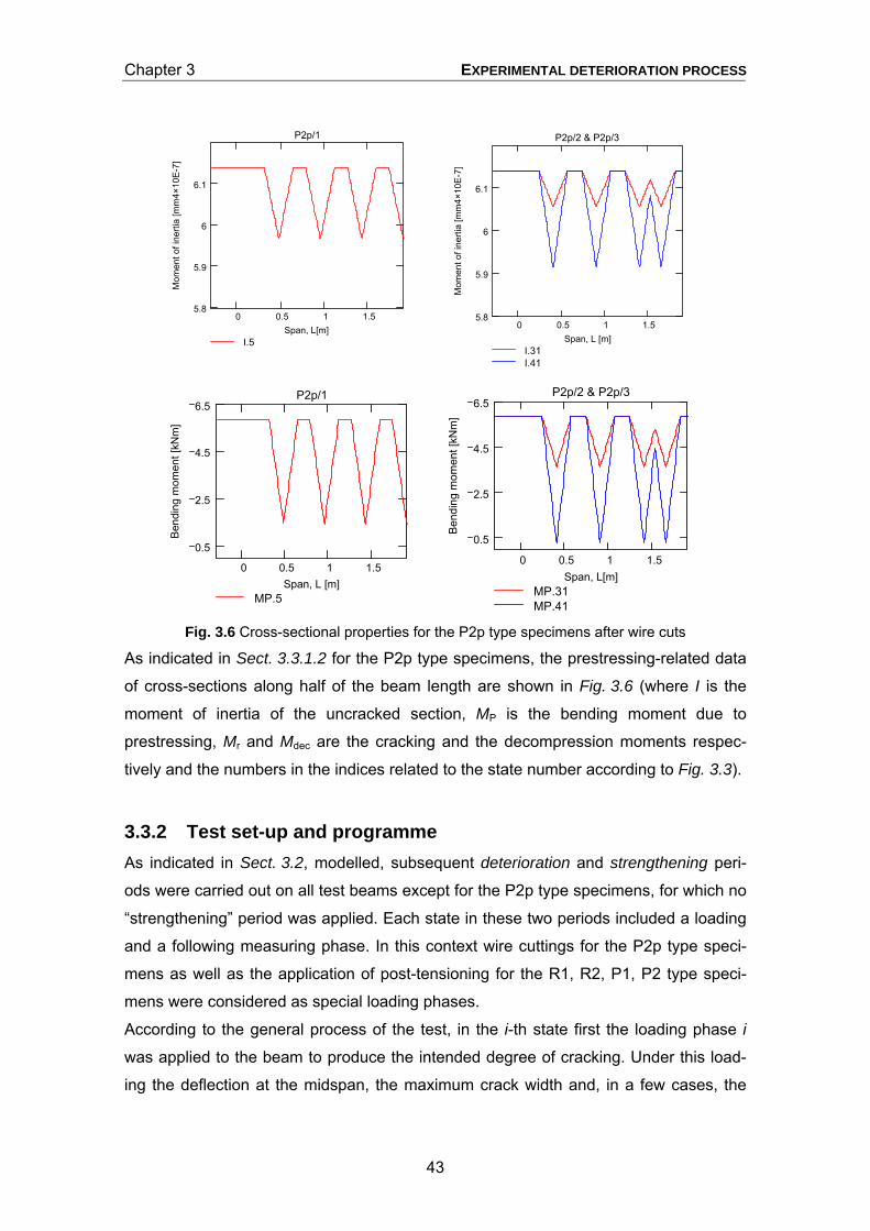
Chapter 3 EXPERIMENTAL DETERIORATION PROCESS
43
0 0.5 1 1.55.8
5.9
6
6.1
I.5
P2p/1
Span, L[m]
Mom
ent o
f ine
rtia
[mm
4×10
E-7
]
0 0.5 1 1.55.8
5.9
6
6.1
I.31I.41
P2p/2 & P2p/3
Span, L [m]
Mom
ent o
f ine
rtia
[mm
4×10
E-7
]
0 0.5 1 1.5
6.5
4.5
2.5
0.5
MP.5
P2p/1
Span, L [m]
Ben
ding
mom
ent [
kNm
]
0 0.5 1 1.5
6.5
4.5
2.5
0.5
MP.31MP.41
P2p/2 & P2p/3
Span, L[m]
Ben
ding
mom
ent [
kNm
]
Fig. 3.6 Cross-sectional properties for the P2p type specimens after wire cuts
As indicated in Sect. 3.3.1.2 for the P2p type specimens, the prestressing-related data
of cross-sections along half of the beam length are shown in Fig. 3.6 (where I is the
moment of inertia of the uncracked section, MP is the bending moment due to
prestressing, Mr and Mdec are the cracking and the decompression moments respec-
tively and the numbers in the indices related to the state number according to Fig. 3.3).
3.3.2 Test set-up and programme As indicated in Sect. 3.2, modelled, subsequent deterioration and strengthening peri-
ods were carried out on all test beams except for the P2p type specimens, for which no
“strengthening” period was applied. Each state in these two periods included a loading
and a following measuring phase. In this context wire cuttings for the P2p type speci-
mens as well as the application of post-tensioning for the R1, R2, P1, P2 type speci-
mens were considered as special loading phases.
According to the general process of the test, in the i-th state first the loading phase i
was applied to the beam to produce the intended degree of cracking. Under this load-
ing the deflection at the midspan, the maximum crack width and, in a few cases, the

Chapter 3 EXPERIMENTAL DETERIORATION PROCESS
44
crack pattern was registered. After the loads were removed, the residual deflection was
also registered at midspan. Then the dynamic measuring phase i took place, during
which the first two natural frequencies were determined by using special excitation ef-
fects. Then the (i+1)-th state with the next loading and measuring phases followed.
3.3.2.1 Loading phases The cracking states were produced by force-controlled four-point bending according to
Fig. 3.7 and Table 3.6. The calculated data of Table 3.6 are based on Sect. 3.3.1.4.
Fig. 3.7 Arrangement of beams under four-point bending
The acting forces (F) were equal to each other and symmetric to the midspan in each
load position. Sliding of the bottom beams on supports during loading was possible at
both ends. The midspan-deflection was measured in each loading phase under loading
and after load removal. A periodic exciter and an acceleration detector were fixed to
the beams as necessary parts of the dynamic measuring equipment (see Fig. 3.11).
Their weights were negligible compared to that of the beams and thus they insignifi-
cantly influenced the dynamic behaviour of the beams. Self-weight (g0=0.39 kN/m) was
the only load on the specimens in states 0 and after the load removal in all other states.
The general concept of choosing the position and the intensity of acting forces in the
subsequent states was to produce gradually increasing flexural cracking in the beams.
According to this concept, flexural cracking is:
• present in a place where the bending moment is higher than the decompression
moment (prestressed beams) and has previously exceeded the cracking moment;
• intensified if the length of sections containing cracks and/or the crack sizes are in-
creased.
t
trlt
tr Lr
~L/5
acceleration detector
l periodic exciter
~L/5 k k
Lb
deflection indicator
Mr
Mmax M
L
FF

Chapter 3 EXPERIMENTAL DETERIORATION PROCESS
45
Table 3.6 Data of loading phases
Load Length of the cracked zone Bending moment ratios at midspan Beam Mark of the deterioration
state F [kN] l [m] Lr [m] Mmax/Mr Mmax/MRd Mmax/MRm
0 0 - 0 0.16 0.055 0.039 1 5.13 0.5 2.07 2.33 0.81 0.57 2 6.63 1.0 2.31 2.45 0.85 0.60 3_1 8.13 1.5 2.47 2.33 0.81 0.57 3 3_2 11.13 1.5 2.66 3.13 1.09 0.76
4 9.63 1.0 2.66 3.48 1.22 0.85
P1
5 8.13 0.5 2.66 3.60 1.26 0.88 0 (for all P2 beams) 0 - 0 0.20 0.043 0.029
1/23 (for P2/2 & P2/3) 2.13 0.5 1.19 1.24 0.26 0.17 1/3 (for P2/3) 4.38 0.5 2.43 2.33 0.49 0.33 1 1/12 (for P2/1 & P2/2) 6.13 0.5 2.79 3.18 0.66 0.45
2/12 (for P2/1 & P2/2) 7.13 1.0 2.92 3.14 0.66 0.44 3/3 (for P2/3) 8.13 1.5 3.02 2.95 0.62 0.41 3
3/12 (for P2/1 & P2/2) 8.63 1.5 3.07 3.12 0.65 0.44 4/12 (for P2/1 & P2/2) 11.13 2.0 3.22 3.15 0.66 0.44
4/3_1 12.13 2.5 3.27 2.52 0.53 0.35 4 4/3 (for P2/3)
4/3_2 16.38 2.5 3.40 3.33 0.70 0.47 5/12 (for P2/1 & P2/2) 11.13 1.5 3.22 3.97 0.83 0.56 6/12 (for P2/1 & P2/2) 11.13 1.0 3.22 4.78 1.00 0.67
P2
7/12 (for P2/1 & P2/2) 11.13 0.5 3.22 5.60 1.17 0.79 0 (for all R1 beams) 0 - 0 0.21 0.100 0.069
1_1 2.13 0.5 1.29 1.28 0.61 0.42 1 (for all R1 beams)1_2 4.13 0.5 2.41 2.29 1.09 0.74
2 (for all R1 beams) 6.13 1.5 2.83 2.36 1.12 0.77 3_1/4 (for R1/4) 10.63 2.5 3.22 2.32 1.10 0.75 3_1/2 (for R1/2) 10.88 2.5 3.23 2.37 1.12 0.77 3_1 3_1/13 (for R1/1 & R1/3) 11.13 2.5 3.24 2.41 1.15 0.78 3_2/4 (for R1/4) 12.13 2.5 3.29 2.61 1.24 0.85 3_2 3_2/123 (for R1/1&/2&/3) 14.13 2.5 3.35 3.01 1.43 0.98 4/3 (for R1/3) 8.38 1.5 3.35 3.15 1.49 1.02 4 4/124 (for R1/1 & /2 & /4) 8.63 1.5 3.35 3.23 1.54 1.05 5/123 (for R1/1 & /2 & /3) 5.88 0.5 3.35 3.17 1.50 1.03
R1
5 5/4 (for R1/4) 6.13 0.5 3.35 3.29 1.56 1.07
0 0 - 0 0.21 0.070 0.047 1_1 2.13 0.5 1.22 1.25 0.42 0.17 1 1_2 4.13 0.5 2.37 2.23 0.75 0.51
2 6.13 1.5 2.80 2.30 0.78 0.53 3_1 11.13 2.5 3.23 2.35 0.79 0.54 3 3_2 14.13 2.5 3.34 2.93 0.99 0.67
4 12.13 1.5 3.34 4.34 1.47 0.99
R2
5 8.63 0.5 3.34 4.43 1.49 1.01 0 0 - 0 0.05 0.036 0.023 1 9.13 0.5 0.58 1.03 0.82 0.53 2 11.63 1.5 0.58 0.92 0.73 0.47 Mmax/Mdec.4 Mmax/Mr.4 Mmax/MRd.4 Mmax/MRm.4
56 6.13 1.5 1.75 1.01 0.80 0.55
P2p/1
5 57 8.13 1.5
see Fig. 3.82.28 1.31 1.04 0.71
0 0 - 0 0.05 0.036 0.023 1 16.13 0.5 1.96 1.78 1.42 0.92 Mmax/Mdec.2 Mmax/Mr.2 Mmax/MRd.2 Mmax/MRm.2
for P2p/2 8.13 2.5 0 0.73 0.52 0.39 0.26 31 for P2p/3 11.13 2.5 0 0.97 0.69 0.52 0.35
Mmax/Mdec.5 Mmax/Mr.5 Mmax/MRd.5 Mmax/MRm.5
for P2p/2 8.13 1.5 3.99 1.76 1.54 1.07
P2p/2 &
P2p/3
41 for P2p/3 7.63 1.5
see Fig. 3.83.76 1.65 1.46 1.01

Chapter 3 EXPERIMENTAL DETERIORATION PROCESS
46
Fig. 3.8 shows the associated moment lines of each loading phase as well as levels of
cracking (Mr) and decompression (Mdec) moments for the P1 and each of the P2p
specimens along one half of the beam lengths. As
mentioned in Sect. 3.3.1.2, the sudden changes in the
Mr and Mdec lines for the P2p type specimens repre-
sent the effects of wire cuts. For the P1, P2, R1 and
R2 beams first the length of the cracked zone (Lr in
Table 3.6) had been gradually increased (in the first
deterioration states) then the crack sizes were signifi-
cantly opened (last states). Loading phases with
Mmax/MRd values smaller than 1.0 represent usual load
cases in practice, but phases when MRd<Mmax<MRm
are not relevant from a practical point of view rather
are able to model structural behaviour close to bend-
ing failure. The same loading phases were applied for
each specimen within the P1 and R2 beam families.
0 0.5 1 1.5
10123456789
10111213141516
M.0M.1M.56M.57Mcr.5Mdec.5
P2p/1
Span, L [m]
Ben
ding
mom
ent,
M [k
Nm
]
0 0.5 1 1.5
2
3
8
13
18
23
28
M.0M.1M.31M.41Mcr.31Mcr.41Mdec.31Mdec.41
P2p/2
Span, L [m]
0 0.5 1 1.5
2
3
8
13
18
23
28
M.0M.1M.31M.41Mcr.31Mcr.41Mdec.31Mdec.41
P2p/3
Span, L [m]
Fig. 3.8 Bending moment lines in the loading phases for the P1 and the P2p type specimens
0 0.5 1 1.5
1
0
1
2
3
4
5
6
7
8
9
10
11
12
13
14
15
16
McrM.0M.1M.2M.31M.32M.4M.5
P1
Span, L [m]
Ben
ding
mom
ent,
M [k
Nm
]

Chapter 3 EXPERIMENTAL DETERIORATION PROCESS
47
For a few specimens within the P2 and R1 beam families, several load phases were
modified in order to investigate minor aspects. For example, for the P2/3 beam the
cracked length extension and the crack size increase were simultaneously produced in
each subsequent state. For the R1/1-3 beams, no significant damage by crack size
increase was produced after the maximum cracked length was reached while this was
not the case for the R1/4 specimen.
A relatively small number of loading phases was introduced to the P2p type
(prestressed) beams. In these cases the main focus was the investigation of tendon
breaks, which was modelled by wire cuts according to Sect. 3.3.1.2. Note that states in
which wire cuts were made are missing from Table 3.6 (such as 3, 41-44 and 5-55 for
the P2p/1 beam and states 2, 3 and 4 for the P2p/2&3 beams). Although all cracks
should have theoretically closed due to prestress during the load removal after state 1,
the basic strategy was still to produce very small cracking before the wire cuts for the
P2p/1 beam and, just the opposite of that, large cracking for the P2p/2&3 beams (as
shown by the M1 lines in Fig. 3.8). The number of cut wires as well as the gradation in
cutting was different (fewer cuts and less rapid cutting rate for the P2p/1 specimen).
Another aspect was to apply states with a loading phase
(state 31 and 41) immediately after states with wire cuts
(state 3 and 4) for the P2p/2&3 beams and no states
with loading phases between states with wire cuts
(states 41-55) for the P2p/1 beam.
Regarding the strengthening states (6p-8p), the strategy
was first to eliminate cracking from the significantly dete-
riorated beams by external post-tensioning (state 6p)
and then to increase the tensioning intensity (states 7p &
8p). The specimens concerned and the process itself is
detailed in Sect. 3.3.1.3 and Table 3.6. Fig. 3.9 shows
the bending moment (M) (under self-weight and post-
tensioning) and the associated decompression moment
(Mdec) lines in states 6p-8p for the half length of the P1
beam (a similar tendency in the M/Mdec ratio was also
observed in the corresponding states for the P2/1&2,
R1/4 and the R2/1 specimens). To have reference data
with regard to the intensity of applied post-tensioning, the relevant Mdec/MRd ratios have
been calculated and included in Table 3.5.
0 0.5 1 1.5
543210123456789
101112131415161718
M.0Mdec.6pM.6pMdec.7pM.7pMdec.8pM.8p
P1
Span, L [m]
Ben
ding
mom
ent,
M [k
Nm
]
Fig. 3.9 Strengthening states for the P1 beam

Chapter 3 EXPERIMENTAL DETERIORATION PROCESS
48
3.3.2.2 Dynamic measuring phases Each state, independently of the preceding loading phase (either a four-point loading or
a wire cut or a post-tensioning), ended in a measuring phase with the aim of determin-
ing the first two natural frequencies. The numerical values of natural frequencies were
obtained statistically from the analysis of signals, which were recorded, transformed
and stored in situ by the appropriate measuring equipment. The vibration signals were
recorded in two ways: in the first case under the free vibration of beams and in the sec-
ond case under a nearly harmonically excited vibration of beams being very close to
resonance.
Measuring equipment and device settings
The measuring equipment included an accelerometer (type Hottinger B3-5) fixed to the
beam at about L/5 distance from one of the supports according to Fig. 3.7. Its position
was chosen by considering on one hand to avoid coincidence with acting forces under
four-point loading as well as the close vicinity of nodes of expected mode shapes dur-
ing vibration and on the other hand to obtain as large amplitudes as possible in order to
better measurability. During the measuring process, the vibration signals produced by
the accelerometer went to an analyser (Tektronix 500), which first recorded the accel-
eration-time (a-t) function then immediately made a fast Fourier transform (FFT) and
directly produced its frequency spectrum.
According to the procedure of the fast Fourier transform, the recorded a-t function is
approximated in discrete (sample) points by the linear combination of “basic” trigono-
metric time functions with unit amplitudes and different frequencies (fbi). The frequency
spectrum is defined as a relationship between the frequencies of basic functions and
their associated relative weights in the linear combination at the best fit. The smallest
basic frequency (fb1) is equal to the reciprocal of the total length of the time function to
be approximated (T [s]) and the others are multiples of fb1, therefore the resolution of
the frequency spectrum (∆f) is equal to fb1. The total length of the recorded time func-
tion depends on the sampling frequency (fs) and the number of discrete sampling
points (N). Regarding the sampling frequency, fs ≥ 2,0fmax is recommended according to
Shannon’s rule in order to avoid deformed (false) spectrums where fmax is the highest
frequency to be measured. (In the case of the P1 specimen, the first natural frequency
(f1) was expected below 40 Hz and the second one (f2) below 140 Hz. For the rest of
longer specimens, lower corresponding natural frequencies were expected.) If fixing fs
then N determines the resolution of the frequency spectrum. In this test, most often
fs=512 Hz was used for the measurements of both f1 and f2, which was much higher

Chapter 3 EXPERIMENTAL DETERIORATION PROCESS
49
(fs>3.5f2) than the recommended limit (fs>2.0f2). Because the FFT requires 2n number
of samples to compute 2n-1 number of basic functions, furthermore, frequency spec-
trums with an appropriately high resolution frequency scale were demanded, N was set
as N=4096(=212) for each sample. Due to lower accuracy in fitting basic functions with
high frequencies, the frequency spectrum often becomes deformed (false) in the high-
est frequency domains. For that reason a default setting of the applied analyser was to
calculate only the first 1600 spectrum ordinates, which resulted in a frequency domain
ranging from 0 Hz to flim=1600fb1. The measurable natural frequency had to fall into this
domain thus the device settings had to be chosen accordingly. Finally, the above set
parameters resulted in a total length of a-t functions of T=N/fs=4096/512=8 s, a fre-
quency spectrum resolution of ∆f=1/T=1/8=0.125 Hz and a frequency range limit of
flim=1600∆f=1600×0.125=200 Hz. Considering f1 as being about 1/4-th of f2, sometimes,
in order to improve the resolution of spectrums, fs=256 Hz sampling frequency was
used only for the f1 measurements, which resulted in T=16 s, ∆f=1/T=1/16=0.0625 Hz
and flim=1600∆f=1600×0.0625=100 Hz.
Excitation techniques
The differences between excitation effects used both in practice and for testing pur-
poses were discussed in Sect. 1.3.4. It was also detailed that a simple mechanical im-
pulse, which is often used in practice for excitation purposes, results in more intensive
excitation forces in the lower frequency domain compared to the higher ones (see
Fig. A2.2).
In the test two types of excitation were investigated. The first was a single mechanical
impulse, which is widely used for experimental purposes.
Fig. 3.10 Schematic comparison of excitation forces for the applied techniques
The second was a nearly harmonic effect, by which only the close vicinity of natural
frequencies were excited with about constant excitation force. A scheme on the differ-
ences in magnitudes of the excitation forces for the two applied techniques can be
seen in Fig. 3.10 where k is an integer, τ measures the duration of the impulse within
the T interval of the excitation effect. The reason for the application of these two excita-
f1 f2
F
f
harmonic:~constantimpulse:
~sin(kπτ/T)/(kπτ/T)

Chapter 3 EXPERIMENTAL DETERIORATION PROCESS
50
tion techniques was to analyse their effects on the shape of the resulting frequency
spectrums.
The mechanical impulse was made by a rubber covered mallet to the beam at the sec-
tion symmetric with the fixed accelerometer to the midspan. This impulse was consid-
ered as an approximation of the Dirac-δ effect with A≠∞ and ∆t=τ≠0 (see Fig. A2.2),
thus more intensive excitation was expected for f1 compared to f2.
a) Hottinger B3-5 accelerometer b) Periodic exciter fixed to the beam
Fig. 3.11 Dynamic measuring devices
In the case of the second technique, an exciter was fixed to the beam about symmetri-
cally with the accelerometer to the midspan as shown in Fig. 3.11. The magnitude of
the excitation force could be varied by either driving cap screws with different lengths
perpendicularly into the rotating axle or by changing the revolution of the exciter. Due
to the pure circular movement of the eccentric mass, the exciter with constant revolu-
tion provided a harmonic, sinusoidal excitation force. During the measuring process,
the revolution of the exciter was slightly altered in such a way that the resulting excita-
tion frequencies varied in the close vicinity of the expected natural frequencies (see
Fig. 3.10). The variation in intensity of the excitation force over this very narrow excita-
tion frequency range (max. 1 Hz) could be taken as negligible. However, considering
the existing degree of structural damping of the beam as well as the revolution needed
to match the excitation frequency to the natural frequency, the magnitude of the excita-
tion force could be controlled by the appropriate selection of the rotational mass to-
gether with its eccentricity. Depending on the natural frequency to be measured, differ-
ent cap screws were applied to keep the amplitudes in the a-t function within accept-
able limits. When the excitation frequency coincided with the natural frequency of the
beam, resonance effects occurred, which were clearly visible as sudden amplitude in-
creases in the plotted a-t function of vibration. At those moments, the magnitude of
amplitudes in the a-t function belonging unambiguously to resonance effects could be
identified and then, during the measurement, only parts of a-t function containing ampli-
tudes close to that measure were recorded for further analysis.
Chapter 3 EXPERIMENTAL DETERIORATION PROCESS
51
3.4 SIGNAL PROCESSING
The evaluation of the recorded a-t functions took place in two steps. First the frequency
spectrums were produced still by the analyser then a statistical analysis of them was
carried out manually. In the following, the main aspects of this evaluation process as
well as the numerical values of the obtained natural frequencies will be introduced.
3.4.1 Computing individual frequency spectrums Getting the beam into vibration with impulse excitation and thereafter letting it move
under free vibration, the signs of excitation in the structural response quickly (after a
few periods) diminish down to an ignorable level and the signs of free vibration become
dominant. Because of this dominance, the relative weight of especially the natural fre-
quency (associated with the mode, on which the damped free vibration runs) and, due
to signal imperfections, of frequencies close to the natural frequency will be signifi-
cantly higher in the frequency spectrum compared to others which are poorly repre-
sented in the free vibration. The applied length of the recorded a-t functions (T) in-
cluded many impulses related, subsequent free vibrating time periods. However, note
that irregularities are present in the a-t functions at moments when the impulses are
activated and that curve fitting to the a-t function becomes difficult and unreliable at
ranges with very small amplitudes because disturbing effects of external noises and the
influence of structural damping become more intensive. One of the recorded a-t func-
tions belonging to state 0 of the P1 specimen and part of its associated frequency
spectrum containing f1 is shown in Fig. 3.12 (fs=256 Hz, ∆f=0.0625 Hz) in the case of
impulse excitation.
Fig. 3.12 Time function due to impulse excitation and its associated frequency spectrum
If using the harmonic excitation technique, the opposite takes place regarding the
structural response. Because in this case the excitation is continuous in time, the exci-
tation frequencies are dominant in the structural response and the natural frequencies

Chapter 3 EXPERIMENTAL DETERIORATION PROCESS
52
disappear from it very quickly (after the first few periods). If intending to measure a
natural frequency, as many coincidences as possible have to be induced between the
excitation and the natural frequency by altering the excitation frequency accordingly
during the recorded time period. Coincidences result in resonance effects. Having
many resonance effects in the a-t function, the relative weight of the associated natural
frequency will be increased in the frequency spectrum. If the recorded a-t function in-
cludes no real coincidence (resonance effect) then the related frequency spectrum will
be deceiving because the frequency with the highest ordinate will be the most domi-
nant excitation frequency instead of the natural frequency. One of the recorded a-t
functions belonging to the same state as for Fig. 3.12 and part of its associated fre-
quency spectrum containing f1 is shown in Fig. 3.13 (fs=256 Hz, ∆f=0.0625 Hz) in the
case of harmonic excitation.
Fig. 3.13 Time function due to harmonic excitation and its associated frequency spectrum
Note that the same frequency value at the peak ordinates on Fig. 3.12 and Fig. 3.13 is
not by chance but, of course, also not a necessity for spectrums representing individual
measurements.
Observe for Fig. 3.13 on one hand that the ratio of the highest amplitude (presumably
belonging exactly to resonance effects) to each of the other ordinates remained below
2.5 throughout the full a-t function, which indicated a structural response really close to
resonance. On the other hand, the magnitude of the maximum amplitude in the a-t
function was adjusted to about the same degree as for the impulse excitation by ap-
propriately controlling the excitation force. Also note that when using the same device
settings for the frequency spectrum computations for both types of excitations, a more
reliable (much higher relative weight of the peak ordinate and no secondary local max.
ordinates next to the peak) and a bit narrower (especially in the close vicinity of to the
peak ordinate) spectrum was obtained from the a-t function of the harmonically excited
vibration.

Chapter 3 EXPERIMENTAL DETERIORATION PROCESS
53
3.4.2 Computing average frequency spectrums It was seen in Sect. 3.4.1 and Sect. 3.3.2.2 that the “correctness” of natural frequencies
obtained from individual frequency spectrums significantly depends on the excitation
input for both types of excitation. For the impulse excitation, the reasons are the lower
excitation force in the higher frequency domains, the irregularities in the a-t function at
impulse activation points and the unreliability of free vibration at ranges with very low
amplitudes. For the nearly harmonic excitation input, the main reason is the imperfect
coincidence between the excitation and the natural frequency during the recorded a-t
function. Therefore, a statistical analysis, during which the individual frequency spec-
trums have been averaged manually, was carried out for both types of excitation which
resulted in the average frequency spectrums. For each state of the beams, a minimum
of 30 individual frequency spectrums were included in this process. Because averaging
decreases the relative weight of non-regular frequencies to a much higher degree than
that of frequencies close to the natural frequencies, the reliability of natural frequencies
given by these average frequency spectrums is expected to improve significantly in
comparison with that given by the individual spectrums.
Fig. 3.14 shows the resulting average frequency spectrums belonging to state 0 of the
P1 beam computed to determine f1 and for both types of excitation.
a) From impulse excitation b) From harmonic excitation
Fig. 3.14 Average frequency spectrums for the first natural frequency (f1)
The average spectrum belonging to the impulse excitation (Fig. 3.14a) shows only
slight changes (in shape far from f1 and in the value of f1) compared to the correspond-
ing individual spectrum shown in Fig. 12. The standard deviation (SD) of frequencies
belonging to the maximum ordinates in the individual spectrums is 0.144 Hz. Addition-
ally, the general shape of the spectrum line, the number and positions of local peaks
next to f1, the relative weight of both local peaks and f1 itself as well as the width of the
peak region in the spectrum line around f1 (~0.5 Hz) are almost unchanged. Based on
this, in the case of impulse excitation, it can be concluded that:

Chapter 3 EXPERIMENTAL DETERIORATION PROCESS
54
• the recorded individual a-t functions regularly contain frequencies which differ from
the natural frequency, represent the imperfectness of structural response under
free vibration and are identified as secondary peaks with unchanged position and
about constant relative weight in the frequency spectrum.
• the individual frequency spectrums are able to provide a relatively good estimation
of f1 with relative weights significantly higher than that of secondary peaks.
• consequently, the average frequency spectrum does not improve the reliability of f1
significantly in comparison with the individual spectrums.
However, the average spectrum belonging to the harmonic excitation (Fig. 3.14b)
shows visible changes compared to the individual spectrum shown in Fig. 13. The SD
of frequencies belonging to the maximum ordinates in the individual spectrums is
0.152 Hz. The relative weight of f1 decreased, the position of f1 shifted to a greater ex-
tent than experienced for the impulse excitation and the width of the peak region in the
spectrum line around f1 became wider. The conclusions for the harmonic excitation are
that:
• the resulting spectrums (both individual and average) are effectively able to filter
out frequencies which differ from the natural frequency.
• the individual frequency spectrums give a bit less reliable estimation of f1 than ex-
perienced for the impulse excitation.
• the average frequency spectrum improves the reliability of f1 in comparison with the
individual spectrums.
However, the picture changes considerably when analysing average frequency spec-
trums related to f2 and belonging to state 0 of the P1 beam as shown in Fig. 3.15. The
same excitation techniques, the same measuring equipment and procedure as well as
the same computational process were applied as for the determination of f1.
a) From impulse excitation b) From harmonic excitation
Fig. 3.15 Average frequency spectrums for the second natural frequency (f2)

Chapter 3 EXPERIMENTAL DETERIORATION PROCESS
55
Using impulse excitation (Fig. 3.15a) it can be seen that the peak region in the spec-
trum line around f2 became much wider than that around f1. Additionally, regular fre-
quencies similar to that in Fig. 3.14a existed and were represented as secondary peaks
with high relative weights in the average spectrum close to the natural frequency. The
differences between relative weights belonging to the natural frequency and to secon-
dary peaks were relatively small. However, the SD of frequencies at maximum ordi-
nates in the individual spectrums resulted in 0.234 Hz, which, considering the magni-
tude, was quite acceptable. These facts indicated a bit lower reliability in the value of f2
compared to f1 if using impulse excitation input.
In using harmonic excitation, an average spectrum similar to that for f1 was obtained,
although the peak region around f2 became wider (~3.0 Hz) than that for f1 (~0.5 Hz).
However, a narrow interval of frequencies before f2 with non-negligible relative weights
may be observed as a secondary peak. Its existence is supported by the fact that the
SD of frequencies at maximum ordinates in the individual spectrums resulted in
0.650 Hz, which was more than four times the corresponding SD for f1.
If further analysing the average frequency spectrums related to f2 as shown in
Fig. 3.15, two main issues should be discussed regarding the aspects set previously for
average spectrums related to f1. The first is the significant widening of the spectrum line
around f2 (Fig. 3.15a) compared to that for f1 (Fig. 3.14a) when using impulse excita-
tion. This, as an addition to the related discussion on the individual spectrums in
Sect. 3.4.1, may be explained by the following two reasons:
• the free vibration, following that the excitation impulse has been activated, runs at
the lowest energy mode. Generally, as is the case for these simply-supported
beams, the first mode stores the lowest energy, therefore f1 is expected to be over-
represented in the recorded a-t functions. The f2 may be excited to an acceptable
level only if the impulse effect is activated at places around the highest amplitudes
of the associated 2nd mode. After the first few periods, the vibration returns to the
lowest energy (1st) mode while the highest modes (including the 2nd mode) gradu-
ally diminish. This makes the measurement of modal data associated with higher
modes difficult and less reliable. In contrast with this, the excitation force of the
harmonic excitation can, between certain limits, be adjusted freely, thus f2 may be
excited with as high an excitation force as needed to get “smooth” frequency spec-
trums.
• As discussed in Sect. 1.3.4 and Sect. 3.3.2.2, the excitation force of the impulse
excitation decreases with the frequency according to the sin(x)/x function. Thus f2 is

Chapter 3 EXPERIMENTAL DETERIORATION PROCESS
56
less intensively excited and, consequently, less represented in the subsequent free
vibration than f1.
The second issue is the observed secondary peaks in the average spectrums related
to f2 for both types of excitation. The mode shape associated with f2 is asymmetric with
one internal node at the midspan, thus the two beam halves vibrate in opposite phases.
If the distribution of bending rigidity along the beam length is not exactly symmetric
about the midspan, which may occur e.g. due to non-visible cracks, then the natural
frequency, which is associated with the strictly symmetric mode shape, slightly shifts
and an additional (virtual) frequency appears and represents itself in the frequency
spectrum as a secondary peak with significant relative weight close to the shifted natu-
ral frequency (Huszár, 2009). This effect remains marginal if the whole beam vibrates
in the same phase as in the 1st mode. The presence of this multiple peak is clearly visi-
ble in Fig. 3.15b for the harmonic excitation but is partly masked by the other above-
mentioned secondary frequencies in Fig. 3.15a for the impulse excitation. However,
using harmonic excitation, the presence and the intensity of the less dominant peak
may also be deceiving in cases when incorrectly coinciding the excitation frequency
with the frequency associated with the dominant peak. The high SD and the intensive
secondary peak before f2 in Fig. 3.15b support these suppositions.
3.4.3 Computing the average of natural frequencies based on indi-vidual spectrums Sect. 3.4.2 drew attention to the presence of multiple peaks around f2 in the computed
average frequency spectrums and introduced the reasons behind them. Also being
aware of the fact that if a multiple peak occurs, none of the local sub-peaks in the mul-
tiple peak corresponds to the exact natural frequency, which is associated with a
strictly symmetric mode shape and represented as a single, narrow peak in the aver-
age frequency spectrum, the question remains: what to consider as a natural frequency
during the evaluation process when multiple peaks exist and, moreover, when the local
sub-peaks fall relatively far from each other. The question is even more stressed be-
cause asymmetry in the crack pattern is relevant, likely and actually not controllable
during the experimental deterioration process (and also in practice). A typical example
is shown in Fig. 3.16 which introduces average frequency spectrums belonging to state
4 of the P1 beam for both types of excitation. It can be seen that the frequency differ-
ence between local sub-peaks in Fig. 3.16a is ~7%. For deterioration states with sig-
nificant cracking, similar average frequency spectrums were obtained.

Chapter 3 EXPERIMENTAL DETERIORATION PROCESS
57
a) From impulse excitation b) From harmonic excitation
Fig. 3.16 Average frequency spectrums with significant multiple peaks around f2 (state 4 of P1)
In order to numerically eliminate the multiple peaks and be able to set f2 for further
evaluation and for comparability reasons, it was decided to consider f2 as the average
of frequencies associated with the maximum ordinates in the individual frequency spec-
trums. The reasons behind this decision were as follows:
• for average frequency spectrums without multiple peaks (typical around f1) the
difference between the average of frequencies associated with the maximum
ordinates in the individual frequency spectrums (henceforth in this section
shortened as average frequency) and the frequency associated with the maxi-
mum ordinate in the average frequency spectrum remains marginal even if the
“hill” around the peak in the average spectrum is wide.
• due to the mentioned frequency shifts in the vicinity of multiple peaks, the aver-
age frequency value falls certainly closer to the exact value of the natural fre-
quency, which is associated with strictly symmetric mode shape and repre-
sented as a single, narrow peak in the average frequency spectrum, than either
of the duplicated peaks.
• for harmonic excitation, the number of false individual spectrums (which derived
from incorrect coincidence of the excitation frequency with one of the sub-peaks
in the average spectrum) relative to the total number of individual spectrums
can be considered as a stochastic parameter that depends first of all on the
abilities of the operator, who adjust the excitation frequency to cause resonance
effects. Presumably this stochastic parameter nearly identically influences the
positions of sub-peaks in the average spectrum as well as the above average
frequency because the individual spectrums are common input for both. There-
fore no additional uncertainty is imported when dealing with the average fre-
quency calculated simply on the basis of individual spectrums instead of sub-
peaks in the average spectrum.

Chapter 3 EXPERIMENTAL DETERIORATION PROCESS
58
In order not to lose information on the presence of multiple peaks when using the aver-
age frequency values, the associated SD values will also be calculated. If frequencies
associated with sub-peaks in a duplicated peak significantly differ from the average
frequency, then the magnitude of SD values clearly reflects it (the higher the SD the
more dominant the presence of the duplicated peak in the average spectrum). The SD
associated with f2 after state 4 of the P1 beam (the related frequency spectrums are
shown in Fig. 3.16) resulted in 4.125 Hz (!) for impulse excitation and 1.546 Hz for
harmonic excitation, which were much higher than the previously (in Sect. 3.4.2) calcu-
lated corresponding SD for state 0 of the same beam (the frequency spectrums belong-
ing to state 0 of the P1 beam without significant duplicated peaks are shown in
Fig. 3.15).
3.5 RESULTS OF FREQUENCY MEASUREMENTS Following the procedure detailed in Sect. 3.3.2 and applying the signal evaluation tech-
nique discussed before in Sect. 3.4, the measured values of the first (f1) and the sec-
ond (f2) natural frequencies of beams belonging to states in the deterioration period
listed in Fig. 3.3, Table 3.4 and Table 3.6 are included in Table 3.7a-e. The frequency
results belonging to states in the strengthening period (states 6p, 7p and 8p, in which
post-tensioning was applied) will be analysed separately in Chapter 5.
3.5.1 Natural frequencies for the deterioration states In the case of the P1 beam, the recorded vibration signals derived from both impulse
and harmonic excitations according to Sect. 3.3.2.2 were evaluated according to
Sect. 3.4.1-3.4.3. The f1 and f2 values in Table 3.7a correspond to averages of 30 fre-
quencies each associated with the maximum ordinates in the related individual fre-
quency spectrums (average frequencies based on 30 individual frequency spectrums).
The associated SD values (s1 and s2 respectively) are also given in Table 3.7a; their
highest values are bold-faced. Table 3.7a Measured values of natural frequencies and the associated SD for the P1 beam

Chapter 3 EXPERIMENTAL DETERIORATION PROCESS
59
The last two columns of Table 3.7a contain the relative difference between the corre-
sponding frequencies computed from signals, which resulted from different types of
excitation. As shown, it remains below 0.6% for f1 and 3% for f2 in each state. This rela-
tive difference for f1 is quite acceptable and demonstrates that both types of excitation
can reliably be used for experimental purposes if a suitable statistical evaluation proc-
ess is applied. In states when the highest relative differences occurred (mostly for f2)
the corresponding SD values were also high. This clearly indicates the presence of
multiple peaks in the frequency spectrums as discussed in Sect. 3.4.
In light of the good coincidence between the determined natural frequencies obtained
from signals with different excitation inputs for the P1 beam, it was generally decided to
use signals derived only from the impulse excitation for further investigation purposes.
When significant multiple peaks in the individual frequency spectrums occurred (in the
case of high SD values), further evaluations were carried out to find the probable rea-
sons behind them by the use of signals derived from harmonic excitation (see further
comments to this in Sect. 3.5.2). In order to spare the available storage capacity and to
reduce the necessary computational effort, the number of individual spectrums, on the
basis of which the average frequencies were calculated, was reduced to 10 (from 30,
which was taken into account in the case of the P1 beam). Therefore Table 3.7b-e con-
tain the first two natural frequency values (f1 and f2) computed (similarly to that in Ta-
ble 3.7a for the P1 beam) as the averages of frequencies associated with the maximum
ordinates in the related 10 individual frequency spectrums as well as the related SD
values (see further comments in Sect. 3.5.2). High SD values are bold-faced. Table 3.7b Measured values of natural frequencies and the associated SD for the P2 beams
Table 3.7c Measured values of natural frequencies and the associated SD for the R1 beams

Chapter 3 EXPERIMENTAL DETERIORATION PROCESS
60
Table 3.7d Measured values of natural frequencies and the associated SD for the R2 beams
Table 3.7e Measured values of natural frequencies and the associated SD for the P2p beams
Unfortunately some electronic data have been lost due to unexpected events such as
temporary power loss or disk failure during the test. This was the case between states
0 and 2 for the R2/3 beam as well as in states 41c and 42c for the P2p/1 beam; their
data are missing from Table 3.7.
The analysis of the above frequency results in relation to test variables and the defined
damage indices can be found in Chapter 5.
3.5.2 Evaluation technique applied for multiple peaks In calculating the average of frequencies associated with the maximum amplitudes in
the individual frequency spectrums (average frequencies) together with their SD, the
sudden increase of SD value from a previous acceptable level (< 1 Hz) was found to be
a good indication of mode deformation, and consequently, of multiple (mostly dupli-
cated) peaks in the related frequency spectrums. In states within the deterioration pe-
riod this mode deformation was clearly caused by a non-symmetric crack pattern and,
consequently, non-symmetric bending rigidity distribution along the beam length. Al-
though all beams were geometrically prismatic and the loading was symmetric in each
state (except when tendon cuts were made in state 43c for the P2p/1 beam), uneven
tensile strength of concrete may result in a non-symmetric crack pattern. Sect. 3.4.2
and Sect. 3.4.3 discussed how non-symmetric bending stiffness distribution resulted in

Chapter 3 EXPERIMENTAL DETERIORATION PROCESS
61
duplicated peaks in the relevant frequency spectrums especially for modes with asym-
metric shapes (here the second mode was affected). Sect. 3.4.3 also discussed that if
these sub-peaks fell relatively close to each other and their relative weights were nearly
identical in the average spectrum (this was the case if their relative weight were either
nearly identical or alternately became maximum in the subsequent individual spec-
trums) then the calculation of the average frequency (average of frequencies associ-
ated with the maximum amplitudes in the individual spectrums) together with its SD
was able to reflect on these kinds of duplicated peaks (see Fig. 3.16a) and to be a
good estimation of the real natural frequency (associated with no mode deformation).
However, when the relative weights of the sub-peaks are significantly different in each
individual spectrum and one of them is dominant (this is presumably the case when the
difference in bending stiffness between the two beam halves becomes significant due
to a non-symmetric crack pattern) then the average frequency reflects only the domi-
nant peak with possibly low SD (in cases when the sub-peaks fall relatively far from
each other). This was definitely the situation through states 4, 5, 6 and 7 for the P2/1
beam; Fig. 3.17 shows the average frequency spectrums (based on 10 individual spec-
trums) belonging to state 5.
a) From impulse excitation b) From harmonic excitation
Fig. 3.17 Over and under-represented sub-peaks around f2 in the average frequency spectrums
(state 5 of P2/1)
In calculating the average frequency for f2 and the associated SD based only on sig-
nals derived from impulse excitation according to Sect. 3.5.1, the frequencies resulted
in 85.61 Hz, 83.40 Hz, 83.65 Hz and 76.48 Hz (associated with SD of 0.30, 0.54, 0.29
and 0.60) for states 4, 5, 6 and 7 respectively, which did not fit into the usual decreas-
ing tendency of f2 observed both through previous states of this P2/1 beam and for all
other beams together. The calculated SD values were acceptably low. However, the
average spectrum showed another local peak around 70 Hz with much lower (but the
same order of) relative weight compared to the calculated frequencies around 80 Hz
(Fig. 3.17a). To check this observation, recorded signals derived from harmonic excita-
Chapter 3 EXPERIMENTAL DETERIORATION PROCESS
62
tion were also analysed. Clear resonance effects could be detected around both 70 Hz
and 80 Hz. The computed average spectrum based on ten individual spectrums, five of
which belonged to natural frequencies around 70 Hz and another five, to that around
80 Hz, gave a similar result (Fig. 3.17b). Based on this, it was decided to include indi-
vidual spectrums with frequencies having a maximum relative weight around 70 Hz into
the statistical analysis. The average frequency in Table 3.7b for these states were cal-
culated from 30 data, 15 of which fell into a relatively narrow frequency interval around
80 Hz and another 15 of which fell into a similar interval around 70 Hz. Consequently,
the associated SD values became considerably high but, in accordance with the origi-
nal intention, unambiguously indicated the presence of duplicated peaks. Similar but
less intensive duplications around f2 could be observed in states where the SD values
are bold-faced in Table 3.7a-e.

4 DEFINITION OF DAMAGE
INDICES

Chapter 4 DEFINITION OF DAMAGE INDICES
64
4.1 GENERAL Damage indices are used to express information on the structural behaviour in numeri-
cal form. This chapter deals with the definition, classification, calculation and compari-
son of damage indices related to the investigated test beams. In this research, only
static-based indices are used in accordance with Sect. 2.3. The applicability of model-
based indices is confirmed by the corresponding non-model-based indices through
conformity checks. The defined indices will be used in Chapter 5 to identify crack-
related damage in test beams.
4.1.1 Interpretation of crack-related damage At the moment when a reinforced concrete beam section cracks under flexure, the
strain energy stored previously in the concrete in the tension zone of the section dis-
charges and is immediately transformed first into kinetic energy, which results in a sud-
den deflection increment of the beam, then again into strain energy, which will be
stored by mostly the tension reinforcement. While this strain and the corresponding
tension force develops in the tension reinforcement, a parallel force transmission from
steel to concrete also takes place along the transmission length of the reinforcing bars.
During this latter force transmission, irreversible micro-cracks develop in the concrete
around the bars, which “softens” the concrete zones beyond the crack faces.
If a reinforcing bar at a crack yields then residual strain remains in the bar after load
removal. If this crack often opens and closes afterwards due e.g. to further loading, the
crack gradually deteriorates (grains fall off the crack faces). For the test beams, all the
above events (micro-cracking, plastic strain in bars, crack surface deterioration):
a) dissipate small parts from the energy transmitted to the beam by the acting
forces in the consecutive loading phases. This dissipated energy is directed to
degrade (damage) zones, which are beyond the linear elastic stage, primarily in
the vicinity of cracks (energy-based approach);
b) are mostly irreversible and result in preventing the main crack to perfectly close
after load removal. Open cracks result in local bending stiffness decrease along
the beam length (crack-amount-based approach).
Instead of a theoretical approach, we suppose that:
a) the amount of energy dissipated in the vicinity of cracks is proportional to that
transmitted to the beam by the acting forces in the current loading phase;
b) the extent of bending stiffness decrease is proportional to the extent of crack-
ing, which is measured by the number and the width of individual cracks.
Chapter 4 DEFINITION OF DAMAGE INDICES
65
The following damage indices are defined in accordance with either of the above ap-
proaches.
4.1.2 Practical aspects of damage index definition From a practical point of view, if neglecting accidental events and specially designed
(e.g. over-reinforced) elements, cracking is an obvious, reliable and most frequently
appearing indication of damage for concrete structures being in service. The reasons
behind cracking may be different (see Sect. 1.1.2) such as mechanical forces, re-
strained deformations, long-term or cyclic loads, chemical attacks, environmental ef-
fects, etc; furthermore, the extent of cracking is tightly influenced by many structural
parameters such as intensity and type of subjecting forces, reinforcement ratio, pres-
ence of prestressing, etc. However, cracking is definitely unfavourable from the point of
view of serviceability and durability. Therefore, instead of the reasons behind cracking,
which are of low interest from the point of view of damage identification; the presence
(detection and localization) as well as the extent (quantification) of cracking are more
important information on the deterioration of the structure and, consequently, are aimed
to be addressed.
In this test, cracking was caused and further intensified by simple mechanical effects
(forces and wire cuts). The consecutive loading phases were planned to gradually in-
tensify cracking either by extending the cracked length of the beam or by widening the
already existing cracks. The resulting cracks seriously influenced the structural re-
sponse of the beams. These crack-influenced parts of the structural response or its
consequences (e.g. residual effects after the removal of crack-inducing mechanical
effects) were intended to be indicated by damage indices. Therefore, all damage indi-
ces were such defined to be influenced by cracking.
According to the interpretation of damage indices in Sect. 2.3, the non-model-based
indices were not based on any previous calculation model; they were defined as pa-
rameters, which were directly measured on the beams or deduced from the measured
parameters without any additional model. The model-based indices were based on a
previous static model and obtained from it by calculations.
4.1.3 Local versus global indices A damage index is considered to be local if the value of the index depends on features
belonging to a local zone of the structure. Thus, these indices do not reflect closely on
the structural behaviour of the structure as a whole (their information content on the

Chapter 4 DEFINITION OF DAMAGE INDICES
66
structure is limited). Consequently, from the point of view of damage detection (Level 1)
and localization (Level 2), they are extremely effective when damage happens within
the related zone, but unusable when damage happens outside this zone. Global indi-
ces are generally obtained from structural parameters gathered from many (preferably
all) zones of the structure. Consequently, features of a local zone do not influence the
value of a global index considerably. Global indices may be more suited for damage
detection if the location of damage is unknown, but local indices are more practical if
the potential damage can be localized to a particular zone of the structure.
When using global indices, the effectiveness of damage localization (and maybe quan-
tification) may be increased if not only one but more structural parameters, which are
primarily linked to different zones of the structure, are investigated (and numerically
determined). That is why the first two natural frequencies are simultaneously investi-
gated in this test. Natural frequency shifts are influenced mostly by zones of beams
where the highest amplitudes of the associated mode shapes are located. Therefore,
damage happened around the midspan zone is expected to result in a higher shift in f1
than in f2 and, taking the opposite of this, a higher shift in f2 suggests damage occurred
around the quarters of the beam.
4.1.4 Cumulative versus incrementative indices Some damage indices are definitely intended to measure damage accumulated in the
structure due to previous deteriorating effects. Theoretically, they cannot decrease dur-
ing a deterioration process unless the healing of damage is possible. Healing of cracks
for some civil engineering structures under special service conditions is possible, even
without any repair work, but in this test this scenario is neglected. Therefore, if no new
damage develops in an intermediate stage within a deterioration process then the ap-
plied damage index should be defined so that its value corresponding to this stage is at
least equal to that corresponding to the previous stage. These cumulative indices are
capable in the first place of damage quantification (Level 3).
If a damage index is intentionally used instead for detection purposes (Level 1) then its
increment between the subsequent states has to be deduced. In this case, the incre-
ment becomes equal to zero for states without new damage.
For this test, the applied damage indices are defined according to their incrementative
form but their cumulative form is also discussed.

Chapter 4 DEFINITION OF DAMAGE INDICES
67
4.2 DEFINITION OF DAMAGE INDICES
The following tables contain the numerical values of all non-model-based and model-
based damage indices defined below in Sect. 4.2 and Sect. 4.3. Further comments to
explain the data included in the tables are also given in the relevant sections. Table 4.1a Damage indices for the P1 beam
Table 4.1b Damage indices for the P2 beams
Table 4.1c Damage indices for the R1 beams
Chapter 4 DEFINITION OF DAMAGE INDICES
68
Table 4.1d Damage indices for the R2 beams

Chapter 4 DEFINITION OF DAMAGE INDICES
69
Table 4.1e Damage indices for the P2p beams
4.2.1 Non-model-based indices
For this test, defined in their incrementative forms, the growth of “total length of cracks”
(∆lr), the growth of deflection measured under loading at midspan (∆atot), the growth of
residual deflection at midspan (∆ares) as well as the growth of crack width measured at
midspan (∆w) were used as non-model-based indices.
4.2.1.1 Growth of “total length of cracks” (∆lr)
The length of an individual crack is interpreted as the length of the irregular curve (or
curves for branching cracks) which is outlined on the side face of the beam and stret-
ches from the extreme tension fibre up to the tip of the crack. The total length of cracks
(lr) summarizes the above lengths of individual cracks over the full cracked length (Lcr)
of the beam.
Defining in that way, the total length of cracks may be considered as a damage index
strictly following the crack-amount-based approach according to Sect. 4.1.1 and con-
taining information on the whole structure (global index). Because it is based only on
in-situ measurements, it can be classified as a non-model-based index.
To determine the total length of cracks, the lengths of individual cracks had to be read
directly from the crack pattern. This process consumed considerable time, therefore it

Chapter 4 DEFINITION OF DAMAGE INDICES
70
was gathered only for the P1, P2/1 and P2/2 beams. As an example, Fig. 4.1 shows
the crack patterns recorded on the side faces of the P1 beam.
Fig. 4.1 Crack patterns recorded on the side faces of the P1 beam
The length of the newly-appearing individual cracks as well as the length increment of
existing cracks were recorded under loading phases and cumulated into lr for each de-
terioration state.
Allowing for Sect. 4.1.4, the incrementative form of lr was defined as ( )irir
ir max <−=∆ lll
where irl was the value of lr in the i-th deterioration state and ( )irmax <l was the maxi-
mum of lr values belonging to previous states. The values of lr and of its incrementative
form (∆lr) can be found in Table 4.1 for the related beams.
4.2.1.2 Growth of total (∆atot) and residual (∆ares) deflection at midspan
These damage indices, defined simply as a deflection value or combination of deflec-
tion values, do not strictly follow either approach of Sect. 4.1.1. However, being the
curvature along a section of a cracked beam mostly concentrated in open cracks, the
curvature is very closely linked to both the number of cracks along this beam section
and their widths. Fig. 4.2 schematically shows bending moment (M) versus curvature
(ρ=1/r) relationships for a reinforced (non-prestressed) and a prestressed beam cross-
section. The circled zones symbolize the typical crack-related damage effects of the
cross-sections, which may correspond to a crack for a reinforced cross-section and to
tendon breaks for a prestressed cross-section. Both of them result in sudden curvature
increment on the cross-section level and, furthermore, in deflection increment on the
beam level. These latter deflection increments are intentionally reflected by these indi-
ces. Thus, they may rather be considered as following the crack-amount based ap-
proach according to Sect. 4.1.1.
Since deflection at any (e.g. midspan) cross-section of a beam depends on the magni-
tude and the distribution of curvature along the whole beam, damage indices based
purely on deflection values may be considered as global rather than local indices.
However, the local character of ∆atot and ∆ares, which are linked to the midspan cross-
section, is also obvious if considering load configurations, which cause greater extent
One side
Other side

Chapter 4 DEFINITION OF DAMAGE INDICES
71
of damage in the whole beam and result in smaller deflection at midspan compared to
other load configurations. Because deflection values are fully in-situ-measured parame-
ters and the deduction of ∆atot and ∆ares do not add any model-based information to
them, the ∆atot and ∆ares indices fall within the group of non-model-based indices.
Fig. 4.2 Schematic bending moment versus curvature relationships
According to Sect. 3.3.2, the deflection at midspan (ameasured) was registered under
loading and after load removal for each loading phase. The deflection of beams under
state 0 (self-weight only) was not measured therefore all measured and deduced de-
flection values were related to beam shape already deformed by the self-weight.
Because the deflection indicator was removed before each dynamic measuring phase,
it had to be re-installed before the subsequent loading phase. Therefore, actual deflec-
tion values developed under loading (atot) and after load removal (ares) had to be ob-
tained from the measured (ameasured) values for each loading phase. Accordingly, atot
and ares associated with the investigated state were obtained as the ares value of the
previous state (baseline) plus the ameasured value of the investigated state. This was not
the case for the P2p beams because deflection measurements during wire cuttings
were impossible due to technical reasons. Thus, deflection increments in states be-
longing to individual wire cuts (such states are shown in Fig. 3.3 and marked by “c” in
the state name in Table 3.7) were not registered and, consequently, no baselines were
available for the loading phases of the subsequent states. Therefore, no atot and ares
values were calculated for these subsequent states.
The incrementative form of atot was defined as ( )[ ]{ }0;maxmax itot
itot
itot
<−=∆ aaa where
itota was the value of atot in the i-th deterioration state and ( )i
totmax <a was the maximum
of atot values belonging to previous states. ∆ares was analogously defined. The results
can be found in Table 4.1 for all beams.
1/r
M
prestressed reinforced (non-prestressed)
Chapter 4 DEFINITION OF DAMAGE INDICES
72
4.2.1.3 Growth of crack width at midspan (∆w)
In practice, the measurement of crack width is difficult and its outcome is unreliable.
Many cracks often become not active under increasing load, thus crack width does not
reflect strictly on the load intensity. Furthermore, widths of neighbouring cracks do not
necessarily fall close to each other.
The crack width (w) in a beam cross-section is fully determined by the internal force
and by the geometric, material and reinforcement properties of the cross-section, there-
fore this crack width itself is considered as a typical local index. Actual crack width
measured directly on the beam is categorized as a non-model-based index. It clearly
follows the crack-amount-based approach according to Sect. 4.1.1. In fact, the residual
width of an active crack would be the ideal index to reflect fully on accumulated dam-
age, however, its measurement with acceptable accuracy is practically unrealistic.
For this test, crack width at midspan (w) was measured by microscope with 0.025 mm
accuracy under loading in every state for many (P2/3, all R1 and R2) but not all beams.
The measured w values and the incrementative form of the index (∆w), defined analo-
gously as introduced in Sect. 4.2.1.2 for ∆atot, can be found in Table 4.1 for the related
beams.
4.2.2 Model-based indices
In calculating model-based indices in accordance with Sect. 4.1.1 and Sect. 2.3 for this
test, assumptions were made regarding the loads, the geometry, the materials, the
material law and the structural behaviour. Concerning the first three, nominal values of
acting forces, nominal sizes, mean values of material properties, were used according
to Sect. 3.3. With regard to material law, a linear-elastic stress-specific strain relation-
ship was taken into account without limits in stress or strain, therefore plastic strains
were not addressed by the applied calculation model.
Concerning the structural behaviour, three models were applied. The first was the well-
known Bernoulli-Navier assumption (principle of plane sections) in accordance with the
general beam theory. The further two models were adopted from the Eurocode 2.
One of them was the calculation model of deformations of structural elements, which
was applied in this test to calculate the ρ(x) curvature of cross-sections along the beam
length as follows:
( ) ( ) ( )( ) ( )[ ] ( )
( )xIExMx
xIExMx
IcmIIcm
1x ζ−+ζ=ρ (4.1)

Chapter 4 DEFINITION OF DAMAGE INDICES
73
where x measured the distance along the specimen from one of the supports; II(x) and
III(x) were the moments of inertia of the cross-section at x in linear elastic uncracked
and cracked stage, respectively; M(x) was the subjecting bending moment at x; Ecm
was the mean value of the modulus of elasticity of concrete. ζ(x) was the distribution
coefficient allowing for tension stiffening and calculated as follows:
( ) ( )
2
s
sr1 ⎟⎟⎠
⎞⎜⎜⎝
⎛σσ
β−=ζx
x (4.2)
where β=1 took into account short-term loading; σsr and σs(x) were the stress in the
tension reinforcement calculated on the basis of cracked cross-section due to cracking
moment (Mcr, see Table 3.5) and M(x), respectively.
0 0.5 1 1.5
0.01
0.0022
0.0056
0.0133
0.0211
0.0289
0.0367
0.0444
0.0522
0.06
State 0State 1State 2State 31State 32State 4State 5
P1
Span, L [m]
Cur
vatu
re, 1
/r [1
/m]
0.3 0.25 0.8 1.35 1.9
0.005
0.005
0.015
0.025
0.035
0.045
State 0P cut0State 1State 31State 3State 4State 41
P2p/3
Span, L [m]
Cur
vatu
re, 1
/r [1
/m]
Al k ált á i i L k
Fig. 4.3 Curvature functions for the P1 and the P2p/3 beams
For cross-sections without normal force (reinforced P1, P2, R1 and R2 beams),
II(x)=II=constant and III(x)=III=constant were considered. The ζ(x) was set equal to zero
for cross-sections uncracked earlier or (only for prestressed beams) being under
decompression. For previously cracked reinforced cross-sections (without normal
force) subjected to M(x)<Mcr, ζ(x) was taken to be at least equal to its value in the
previous state. For prestressed (P2p type) cross-sections with no wire cuts and
subjected to M(x)>Mcr, first ρ was calculated at particular cross-sections (ρ(xi)) along
the cracked length of the beam and then linearly interpolated between these ρ(xi) val-
ues for the remaining cross-sections (state 1). In the vicinity of wire cuts, ρ was

Chapter 4 DEFINITION OF DAMAGE INDICES
74
remaining cross-sections (state 1). In the vicinity of wire cuts, ρ was calculated, on one
hand, exactly at the cut (allowing for only the remaining number of wires) and, on the
other hand, at the end of the transmission length on both sides of the cut. For cross-
sections located between these calculation points, both inside and outside the (vicinity
of) cuts, linear interpolation was applied. Fig. 4.3 shows the accordingly calculated cur-
vature functions along the half length of the reinforced P1 and the prestressed P2p/3
beam.
The third structural model was related to crack width calculation. According to this, the
width of a crack (wcalc) in a cross-section was calculated as follows:
wcalc = sr,max (εsm - εcm) (4.3)
where sr,max estimates the maximum crack spacing according to Eq. (4.4):
sr,max = 3.4 c + 0.425 k1 k2 eff,pρφ (4.4)
where c is the concrete cover; φ is the bar diameter; k1 allows for the bond properties of
the reinforcement and k2 takes into account the strain distribution along the cross-
section. k1=0.8 (high bond) was used for reinforcing bars (R1 and R2 beams) and
k1=(0.8+1.6)/2=1.2 (ribbed wires) for prestressing wires (P1, P2 and P2p beams). Due
to bending, k2 was taken as k2=0.5. ρp,eff is the effective steel ratio as follows:
ρp,eff = As/Ac,eff (4.5)
where Ac,eff is the effective tension area of concrete, whose depth is the minimum of
2.5(h-d), (h-x)/3 and h/2 (h and d are the height and the effective depth of the cross-
section, respectively; x is the depth of the compression zone). As represents the area of
longitudinal reinforcement falling within Ac,eff. εsm and εcm are the main strain in the rein-
forcement within the crack and in the (uncracked) concrete between cracks, respec-
tively; the (εsm - εcm) strain difference was calculated as follows:
(εsm - εcm) = ( )
s
s
s
eff,peeff,p
ctmts
6.01
EE
fk
σ≥
ρα+ρ
−σ
(4.6)
where σs is the stress in the outermost bar assuming cracked cross-section. Only addi-
tional stress (∆σs) above the stress associated with zero strain in concrete at the same
level was considered for the prestressed reinforcement (for P2p beams). Due to short-
term loading kt=0.6 was taken. Furthermore, αe=Es/Ecm with Es representing the
modulus of elasticity for steel.

Chapter 4 DEFINITION OF DAMAGE INDICES
75
For this test, defined according to their incrementative form, the growth of deflection
(∆acalc) and the growth of crack width (∆wcalc), both of them calculated at midspan under
loading, as well as the growth of “total of crack sections” (∆Ar) and the growth of inter-
nal strain energy of deformation (∆W) under loading were defined as model-based indi-
ces for each deterioration state on the basis of the above models.
4.2.2.1 Growth of “total of crack sections” (∆Ar)
This index, on one hand, is similar to ∆lr defined in Sect. 4.2.1.1 but based on a previ-
ous calculation model. However, on the other hand, it addresses not only the length of
individual cracks but their widths as well. Therefore, due to its greater information con-
tent on cracking, it is more capable of identifying the growth of crack-related damage.
The section of an individual crack (Ar,i) is interpreted as shown in Fig. 4.4 (hatched
area). The tip of the crack is assumed at that level of the cracked cross-section at
which the flexural tensile strength of concrete (fctm,fl) occurs due to the subjecting loads.
Based on this, the “total of crack sections”, which summarized Ar,i over the cracked
length of the beam, was calculated as follows:
Ar = ∑i,r
i,rmax,r
i,r
LA
ss
(4.7)
where Lr,i measured the cracked length of beams in
the i-th state, scr,i was the distance within Lr,i, along
which wcalc and hr (both included in Ar,i) were averaged.
This index fully complies with the crack-amount-based approach according to
Sect. 4.1.1 and is able to reflect crack-related damage over the whole beam. Conse-
quently, it can be categorized as a global index.
The results can be found in Table 4.1 for all beams. For the prestressed P2p beams,
this index was determined only for states before wire cuttings. For states during and
after wire cuttings, the application of the above-introduced calculation procedure be-
came unrealistic. The incrementative form of the index (∆Ar) was defined analogously
as introduced in Sect. 4.2.1.1 for ∆lr.
4.2.2.2 Growth of calculated midspan deflection (∆acalc)
Similarly to ∆atot defined in Sect. 4.2.1.2, ∆acalc was intended to address the conse-
quences of crack-related damage, which occurred somewhere in the beam, in the
midspan deflection, however, on the basis of calculation models detailed above in
Sect. 4.2.2. Thus, this can also be categorized as a global rather than a local index.
hr
wcalc
fctm,fl Ar,i=hrwcalc/2
Fig. 4.4 Assumed section of an individual crack (schematic)

Chapter 4 DEFINITION OF DAMAGE INDICES
76
In determining this index, first the total deflection at midspan (acalc) was calculated as
follows:
acalc = ( )∫ ⎟⎠⎞
⎜⎝⎛ −ρ−ϕ
2L
0
d22
xxLxL (4.8)
where ρ(x) was the curvature function according to Eq. (4.1); ϕ was the rotation of
cross-section above one of the supports, from which x was measured, and L meant the
beam span. All the acalc values included in Table 4.1 were reduced by acalc0, which was
the calculated midspan deflection in state 0 (self-weight only) and was italicized in Ta-
ble 4.1, in order to express deflection due only to acting forces in each state. Calculat-
ing this manner, acalc became comparable to atot (see Sect. 4.2.1.2).
The results can be found in Table 4.1 for all beams. The incrementative form of the
index (∆acalc) was defined analogously as introduced in Sect. 4.2.1.2 for ∆atot.
4.2.2.3 Growth of calculated crack width at midspan (∆wcalc)
The growth of the calculated crack width at midspan (∆wcalc) is the model-based ana-
logue of ∆w defined in Sect. 4.2.1.3, therefore it can be categorized accordingly. How-
ever, a close coincidence between ∆wcalc and ∆w was not necessarily expected be-
cause of the unreliability of crack width measurement as discussed in Sect. 4.2.1.3.
The results can be found in Table 4.1 for all beams. The incrementative form of the
index (∆wcalc) was defined analogously as introduced in Sect. 4.2.1.3 for ∆w.
4.2.2.4 Growth of internal strain energy (∆W)
The aim of the definition of this index is, on one hand, to provide a full global index, in
which structural behaviour of no local beam parts as well as no specific crack parame-
ters is preferred, and, on the other hand, to strictly follow the energy-based approach
according to Sect. 4.1.1. In fact, this index, similarly to the above model-based indices,
is based on the curvature model introduced in Sect. 4.2.2, however, calculated as a
quantity irrespective of any directly visible or measurable structural characteristic. This
improves its global character but makes controllability (by non-model-based indices)
difficult and, consequently, decreases its robustness.
The idea behind this index is based on the assumption that the resulting damage, as
interpreted in Sect. 4.1.1, in a reinforced concrete beam cross-section, which cracked
earlier under flexure and then again subjected to and deformed by flexure, is propor-
tional to that part of the internal strain energy of the deformation which is incremental to
that occurred due to previous bending deformations. According to this, no newly occur-
ring crack-related damage is assumed if the cross-section is subjected to a bending

Chapter 4 DEFINITION OF DAMAGE INDICES
77
deformation whose internal strain energy is less than that of a previous bending defor-
mation. Also no damage is assumed for uncracked sections which are subjected to a
bending moment less than the cracking moment, because they are assumed to re-
spond fully elastic without any non-linear effect. As shown, this approach always sup-
poses non-linearity for reinforced concrete cross-sections already cracked under flex-
ure when subjected to bending deformation, which was not achieved earlier. In fact,
this non-linearity is aimed to be addressed by this index.
Note that only bending deformation is considered by the above approach. However, it
can be extended to prestressed beams, even if they work under the combination of
axial and bending deformation, if prestressing is considered as an internal action,
which shifts the limit between the uncracked and the cracked behaviour of sections as
well as if the bending deformation due to prestressing is excluded from the subjecting,
external deforming effect. Before the first crack of the prestressed cross-section, no
damage is assumed. After the first crack, when a bending deformation occurs which
was not achieved earlier, the idea supposes crack-related damage even if cracks
(theoretically) close due to prestressing after the deforming effect disappears. In this
test, this concept was applied to the P2p beams.
0 0.5 1 1.5
0.1
0
0.1
0.2
0.3
0.4
0.5
0.6
0.7
State 0State 1State 2State 31State 32State 4State 5
P1
Span, L [m]
Ben
ding
mom
ent ×
Cur
vatu
re, M
/r [k
N]
0 0.5 1 1.5
0.1
0.0833
0.27
0.45
0.63
0.82
State 0 State 1State 31State 41
P2p/3
Span, L [m]
Ben
ding
mom
ent ×
Cur
vatu
re, M
/r [k
N]
Fig. 4.5 Curvature function for the P1 and the P2p/3 beams
The internal strain energy (W) of a bending deformation was defined as follows:
W = ( ) ( )∫ ρr
dL
xxxM (4.9)
Chapter 4 DEFINITION OF DAMAGE INDICES
78
where M(x) and Lr are in accordance with Sect. 4.2.2 and Sect. 4.2.1, respectively, and
ρ(x) is according to Eq. (4.1). Fig. 4.5 shows the calculated M(x)ρ(x) function product
for the half of the reinforced P1 and the prestressed P2p/3 beam (see also Fig. 3.8 and
Fig. 4.3 and note that the integral in Eq. (4.9) works only over Lr).
The results can be found in Table 4.1 for all beams. The incrementative form of the
index (∆W) was defined analogously as introduced in Sect. 4.2.1.2 for ∆atot.
4.2.3 Comparison of non-model-based and model-based indices The use of model-based static indices is justified if their coincidence with reality is con-
firmed. It is essential for practical cases when no in-situ static measurements can be
made to check the calculated indices due to limited accessibility or other technical rea-
sons. In these cases, the applied model-based indices have to be previously verified by
a baseline obtained from previous in-situ measurements. If parallel in-situ measure-
ments may be executed, then parallel non-model based indices can be defined and
compared to the model-based ones to check their conformity.
For this test, two possibilities were available to conduct these checks because parallel
non-model-based and model-based indices were used with regard to deflection and
crack width. Within this framework, the total deflection under loading was both meas-
ured (atot) and calculated (acalc), furthermore, similarly to this, the crack width at
midspan was also measured (w) and calculated (wcalc). These corresponding non-
model-based and model-based data could directly be compared and their coincidence
could be analysed. These data are shown in Fig. 4.6a-d for a few beams, by which the
typical stages of their structural behaviours can be reflected.
Owing to the unreliability of crack width measurements, the comparison of atot and acalc
was more appropriate for the coincidence checks. Generally, with the exception of P2p
beams with cut wires, good coincidence was found while the beams remained fairly
elastic (see both P1 and P2 beams plus the R1/2 beam up to state 3_2), which verified
the suitability of the applied calculation (curvature) model. It was generally observed
that if a higher atot value (compared to the corresponding acalc) was measured immedi-
ately after the first cracks appeared, then generally the atot values slightly exceeded the
corresponding acalc values through all the following deterioration states (typical case for
this is the R1/2 beam), otherwise the acalc values remained higher (see the P1 beam).
Where measured crack width data (w) were available, their acceptable coincidence
with the corresponding wcalc was also observed (e.g. for the P2/3 beam), however, their
ratio provided small useful information. In states of the P2p beams after wire cuttings

Chapter 4 DEFINITION OF DAMAGE INDICES
79
(state 56 and 57 for P2p/1 and state 31 and 41 for P2p/2&3), significantly higher atot
values were measured than the corresponding acalc values, which was in contrast to
that experienced in states before wire cuts (state 1, see Table 4.1e). This suggested
that wire cuts had much more influence on curvature than estimated by the applied
curvature model (in Fig. 4.3).
a) P1 beam b) P2/1 beam
c) P2/3 beam d) R1/2 beam
Fig. 4.6 Conformity check of non-model-based and model-based indices
An interesting situation was observed for the P2/1 beam (Fig. 4.6b). Through states 3
and 4, when the acting forces were located far from the midspan, a virtual hardening in
the measured midspan deflection was experienced in contrast to the calculated behav-
iour. This was the highest difference between atot and acalc experienced among all
beams and was also reflected by the measured natural frequencies (see Sect. 5.3.4 for
the explanation).
Plastic deformation, which was expected in the last states for the R1, R2 and P2p2&3
beams (see Mmax/MRm ratios higher than 1.0 in Table 3.6) but was not reflected by the
applied material law, was clearly experienced for all of the related beams (visible in
Fig4.6d for the R1/2 beam) by the significant increase of the measured atot and w val-
ues in the relevant deterioration states and by their detachment from the corresponding
calculated values.

5 DAMAGE IDENTIFICATION
AND ASSESSMENT OF
MODEL BEAMS

Chapter 5 DAMAGE ASSESSMENT OF MODEL BEAMS
81
5.1 INTRODUCTION The goal of this chapter is to present crack-related damage identification and assess-
ment of the investigated beams on the basis of their first two natural frequencies and
their associated shifts measured in accordance with Chapter 3 and given in Table 3.7.
Damage identification is governed by the damage indices defined in Chapter 4 and
given in Table 4.1. Each level of damage identification will be discussed. The useful-
ness as well as the limits of applicability of static-based damage indices will be demon-
strated.
Damage assessment focuses mainly on crack-related damage. For the originally non-
prestressed (reinforced) beams, the gradual degradation of the beams due to intensify-
ing cracking is assessed by the measured natural frequency shifts in typical deteriora-
tion states. Effects of test variables (see Sect. 2.3.1) on the natural frequency changes
will also be discussed. For the originally prestressed as well as for the post-tensioned
beams, the influence of change in prestress on the natural frequencies of the beams
will be analysed for different extents of previous crack-related damage.
5.1.1 Application of damage indices in experimental damage identi-fication and assessment Damage indices are usually defined to express information on the structural condition
in numerical form. Structural damage changes the structural information given by the
index and, consequently, indicated as a change in the value of the damage index.
Because they do not require an additional structural model, non-model-based indices
are determined from measured structural properties. Therefore, they do not include any
model uncertainty and, for this reason, are more capable of characterizing the behav-
iour of existing structures than model-based indices. However, for existing structures,
the execution of on-site measurements is often difficult due e.g. to accessibility rea-
sons. At that point, model-based indices calculated on the basis of previous static
models are applied to help damage identification. Model-based indices contain informa-
tion on the behaviour of the model of the structure, which is affected by modelled dam-
age in the form of assumed damage cases (e.g. newly formulated cracks, intensifying
existing cracking, changes in support conditions, variation in ratio of internal forces to
capacity). For the identification of existing structures, the use of assumed damage
cases (damage models) being very close to service conditions is essential.
When executing dynamic tests (see Fig. 2.1) on existing structures, dynamic parame-
ters (e.g. f1 and f2) are measured and, if practical, their derivatives (e.g. ∆f1 and ∆f2) are

Chapter 5 DAMAGE ASSESSMENT OF MODEL BEAMS
82
deduced. Dynamic-based damage assessment is carried out if the structural condition
(or any change in it) is deduced from the measured dynamic parameters. To achieve
this,
first the damage has to be identified by (either non-model-based or model-
based) damage indices and then related to the measured dynamic parameters
(or to their derivatives);
then the measured dynamic parameters (or their derivatives) have to be related
to structural parameters which characterize the performance of the (damaged)
structure.
In this test, both non-model-based and model-based indices were defined for experi-
mental purposes. The applicability of model-based indices was verified in Sect. 4.2.3
by checking their coincidence with non-model-based indices. During the identification
phase (Sect. 5.3) mainly the incrementative form of damage indices are applied and
related to shifts (∆f1 and ∆f2) of the measured natural frequencies. Each level of identi-
fication (detection, localization and quantification) is thoroughly discussed. Within the
assessment phase (Sect. 5.4), the structural condition is reflected
on one hand directly by the value of the defined model-based index (∆wcalc, ∆Ar)
or,
on the other hand by performance-based properties defined for each beam in
Sect. 3.3.
Concluding remarks are made in relation to the evaluation of test variables (Sect. 2.3.1)
in the assessment phase with regard to aspects of practical application.
5.1.2 Introduction of test results When conducting damage identification Level 1 (detection) and 2 (localization) are in
focus. The way how the results are introduced should support this concept.
Detection is focused if the incrementative form of damage indices (Sect. 4.1.4) is used,
because any value other than zero of the index indicates a change in the investigated
parameter (here in the natural frequency). If the magnitude of the index is proportional
to the magnitude of the change in the investigated parameter, then this form is very
helpful even in quantifying damage (Level 3). Owing to this, the frequency changes
measured in the i-th state will be drawn as frequency shifts (∆fi) relative to the fre-
quency belonging to the previous state (∆fi=fi-fi-1).
As discussed in Sect. 4.1.3, damage within zones located around the highest ampli-
tudes of the associated mode shape influence the frequency shifts to the highest de-

Chapter 5 DAMAGE ASSESSMENT OF MODEL BEAMS
83
gree. This means that single damage somewhere along the beam is expected to influ-
ence ∆f1 and ∆f2 to a different extent. Therefore, the location is focused if f1 and f2 as
well as ∆f1 and ∆f2 are simultaneously drawn against damage indices.
Fig. 5.1a Natural frequency shifts versus damage indices for the P1 beam
Fig. 5.1b Natural frequency shifts versus damage indices for the P2 beams

Chapter 5 DAMAGE ASSESSMENT OF MODEL BEAMS
84
Fig. 5.1c Natural frequency shifts versus damage indices for the R1 beams

Chapter 5 DAMAGE ASSESSMENT OF MODEL BEAMS
85
Fig. 5.1d Natural frequency shifts versus damage indices for the R2 beams
The f1 and f2 natural frequencies (see Table 3.7) and their deduced shifts (∆f1 and ∆f2)
as well as the defined damage indices (see Table 4.1) in their incrementative form are
drawn in Fig. 5.1 for the related deterioration states of the P1, P2, R1 and R2 beams.
For technical reasons, all quantities in the diagrams of Fig. 5.1 were converted into
percentage. The natural frequencies (f1i and f2i) as well as their shifts (∆f1i and ∆f2i) be-
longing to the i-th state are relative to f0 (the value of f in state 0) for all beams. The
zero axis belonging to ∆f1i and ∆f2i is fixed at 100% (on the left side vertical axes) and,
furthermore, the positive values of ∆f1i and ∆f2i are drawn downwards from this zero
axis. Similarly, the percentage values of incrementative damage indices are relative to
the highest value of the corresponding index (given in Table 4.1), which, in fact, corre-
sponds to the 100% value of the cumulative index.

Chapter 5 DAMAGE ASSESSMENT OF MODEL BEAMS
86
The influence of change in prestress (i.e. the effects of wire cuts) on the frequency
shifts for the prestressed P2p beams as well as the influence of change in post-
tensioning through states 6p, 7p and 8p on the natural frequencies of the related
beams are discussed separately in Sect. 5.4.2 and Sect. 5.4.3.
5.2 ANALYTICAL AND NUMERICAL CALCULATIONS
Despite the fact that the objective of this research is to assess damage without using
dynamic models (see Sect. 2.1.4), this section provides rough estimations of the first
two natural frequencies of model beams on the basis of linear elastic analyses.
Since their determination needs short time and small computation effort, rough estima-
tions may be practical for calibrating the measuring equipment and to select the appro-
priate device settings. For structures with complex shape or with multiple static inde-
terminacies, a priori estimations based on very simple assumptions may help better
understanding of the structural behaviour (e.g. during mode shape identifications).
5.2.1 Analytical estimations Assuming beams uncracked in full length, ignoring side cantilevers beyond the sup-
ports (marked by k in Fig. 3.7) and neglecting structural damping, as simplifications, the
first two natural frequencies may analytically be calculated as follows:
f1I,calc = 4
0
Icm2
21
LgIE
gππ
and (5.1a)
f2I,calc = 4
0
Icm2421
LgIE
gππ
(5.1b)
where g=9.81 m/s2; g0=0.39 kN/m is the self-weight; L is the span; II is the moment of
inertia based on uncracked cross-section and assumed as constant over L; Ecm is the
short-term modulus of elasticity (see Table 3.2). Eq. (5.1a) and (5.1b) resulted in f1I,calc
and f2I,calc given in Table 5.1. The maximum difference of measured frequencies be-
longing to states 0 (no cracks) in Table 3.7 compared to f1I,calc and f2I
,calc was obtained
as +7% and +1% for the P1 beam as well as -26% – -12% and -25% – -8% for the P2,
R1 and R2 beams, furthermore -1% – +4% and -5% – -2% for the P2p beams, respec-
tively. These deviations from f1I,calc and f2I
,calc indicated that the dynamic behaviour of a
real concrete beam could be significantly different from that of an improperly adjusted
calculation model. However, if assuming perfect geometry (L), these frequency devia-
tions were necessary consequences of deviations in either EI or g0 and were clear indi-

Chapter 5 DAMAGE ASSESSMENT OF MODEL BEAMS
87
cations of either insufficient density or existing but invisible micro-cracks in the concrete
material or any hidden defect in the beam. Table 5.1 Analytically calculated natural frequencies
Based on uncracked beam Based on fully cracked beam Beam f1I
,calc [Hz] f2I,calc [Hz] f1II
,calc [Hz] f2II,calc [Hz]
P1 34.05 136.20 10.93 43.72 P2 & P2p 24.79 99.17 11.71 46.85
R1 24.36 97.43 10.79 43.18 R2 24.55 98.18 12.68 50.74
When substituting II in Eq. (5.1a) and (5.1b) with III (fully cracked beam), which is the
moment of inertia on the basis of cracked cross-section, then Eq. (5.1a) and (5.1b)
resulted in f1II,calc and f2II
,calc (see Table 5.1). These values were much smaller than
those belonging to the last deterioration states of beams (even for states when
Mmax/MRm>1.0) given in Table 3.7.
It was concluded that the corresponding fIcalc and fIIcalc values may only be used as
rough upper and lower estimations of natural frequencies for beams damaged by
cracks. However, the magnitude of difference between the measured natural frequen-
cies of a visibly undamaged beam and the corresponding fIcalc values may be informa-
tive regarding the presence of invisible hidden defects in the beam.
5.2.2 Numerical estimations Analytical calculations become difficult if the structural system becomes complicated.
Due to the application of the introduced post-tensioning (see Sect. 3.3.1.3) to the re-
lated, originally non-prestressed beams, the previous simply-supported system was
transformed into a complex, non-symmetric system consisting of the beam itself, the
external strands (without any deviators), the anchorage plates and the jack. This modi-
fication in the structural system resulted in a considerable change of the natural fre-
quencies and made second order numerical analysis necessary when calculating the
natural frequencies at varying post-tensioning force in the strands.
a) Dominant first beam mode b) Dominant second beam mode c) An alternative to b)
Fig. 5.2 Mode shapes of the system including the dominant first and second beam modes
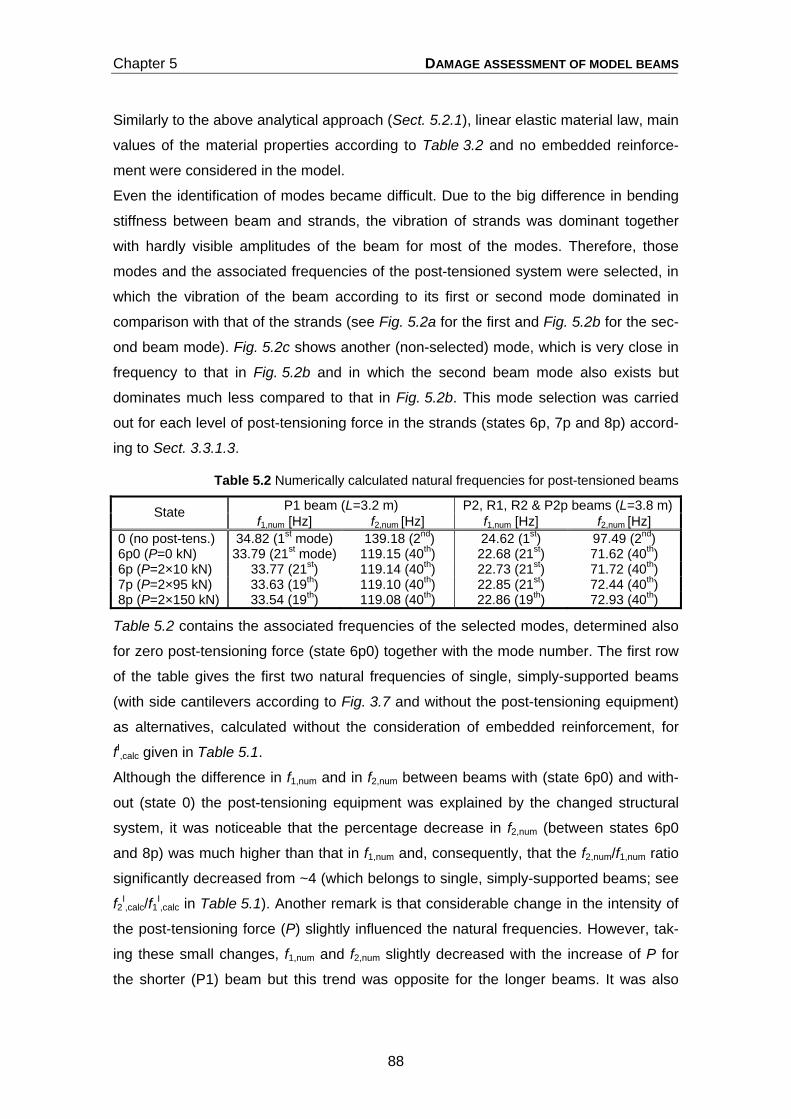
Chapter 5 DAMAGE ASSESSMENT OF MODEL BEAMS
88
Similarly to the above analytical approach (Sect. 5.2.1), linear elastic material law, main
values of the material properties according to Table 3.2 and no embedded reinforce-
ment were considered in the model.
Even the identification of modes became difficult. Due to the big difference in bending
stiffness between beam and strands, the vibration of strands was dominant together
with hardly visible amplitudes of the beam for most of the modes. Therefore, those
modes and the associated frequencies of the post-tensioned system were selected, in
which the vibration of the beam according to its first or second mode dominated in
comparison with that of the strands (see Fig. 5.2a for the first and Fig. 5.2b for the sec-
ond beam mode). Fig. 5.2c shows another (non-selected) mode, which is very close in
frequency to that in Fig. 5.2b and in which the second beam mode also exists but
dominates much less compared to that in Fig. 5.2b. This mode selection was carried
out for each level of post-tensioning force in the strands (states 6p, 7p and 8p) accord-
ing to Sect. 3.3.1.3.
Table 5.2 Numerically calculated natural frequencies for post-tensioned beams
P1 beam (L=3.2 m) P2, R1, R2 & P2p beams (L=3.8 m) State f1,num [Hz] f2,num [Hz] f1,num [Hz] f2,num [Hz]
0 (no post-tens.) 34.82 (1st mode) 139.18 (2nd) 24.62 (1st) 97.49 (2nd) 6p0 (P=0 kN) 33.79 (21st mode) 119.15 (40th) 22.68 (21st) 71.62 (40th) 6p (P=2×10 kN) 33.77 (21st) 119.14 (40th) 22.73 (21st) 71.72 (40th) 7p (P=2×95 kN) 33.63 (19th) 119.10 (40th) 22.85 (21st) 72.44 (40th) 8p (P=2×150 kN) 33.54 (19th) 119.08 (40th) 22.86 (19th) 72.93 (40th)
Table 5.2 contains the associated frequencies of the selected modes, determined also
for zero post-tensioning force (state 6p0) together with the mode number. The first row
of the table gives the first two natural frequencies of single, simply-supported beams
(with side cantilevers according to Fig. 3.7 and without the post-tensioning equipment)
as alternatives, calculated without the consideration of embedded reinforcement, for
fI,calc given in Table 5.1.
Although the difference in f1,num and in f2,num between beams with (state 6p0) and with-
out (state 0) the post-tensioning equipment was explained by the changed structural
system, it was noticeable that the percentage decrease in f2,num (between states 6p0
and 8p) was much higher than that in f1,num and, consequently, that the f2,num/f1,num ratio
significantly decreased from ~4 (which belongs to single, simply-supported beams; see
f2I,calc/f1I
,calc in Table 5.1). Another remark is that considerable change in the intensity of
the post-tensioning force (P) slightly influenced the natural frequencies. However, tak-
ing these small changes, f1,num and f2,num slightly decreased with the increase of P for
the shorter (P1) beam but this trend was opposite for the longer beams. It was also

Chapter 5 DAMAGE ASSESSMENT OF MODEL BEAMS
89
interesting that with increasing P the modes of the system rearranged (the first beam
mode belonged to the 21st mode of the system for lower P then to the 19th mode for
higher P). These trends in comparison with the corresponding measured natural fre-
quencies are further analysed in Sect. 5.4.3.
Even the above results suggested that in practice when any new (structural and/or non-
structural) element is added to an existing structure (e.g. for strengthening purposes),
the changed modal data of the structure have to be registered as a baseline for further
investigations.
5.3 DAMAGE IDENTIFICATION OF MODEL BEAMS
This section deals with damage identification aspects for the tested beams with respect
to the identification levels discussed in Sect. 1.2.
5.3.1 Detection As discussed in Sect. 5.1.2, the incrementative form of damage indices in damage de-
tection is helpful. The success of damage detection by natural frequency measure-
ments depends mainly on the coincidence in shape of ∆f1 and ∆f2 curves with those of
the applied damage indices. For diagrams presented in Fig. 5.1 for the test beams, a
similar shape of ∆f1 or ∆f2 and of the defined indices (∆lr, ∆w, ∆atot, ∆ares, ∆Ar, ∆wcalc,
∆acalc, ∆W) indicates such damage, which is reflected by the ∆f1 and ∆f2 natural fre-
quency shifts.
Generally good coincidence in shape of the applied non-model-based indices (∆lr, ∆w,
∆atot, ∆ares) was found for most of the beams through the full deterioration process. In
some cases, the non-regular deviations of some indices from other indices could be
explained either by the different character (global or local) of the indices or by the unre-
liably appearing first cracks. As an example of the latter, consider states 1 and 2 of the
P2/1 beam. The ∆ares indicated high damage around midspan in state 1 (see also high
∆f1) and very little additional damage in state 2. Meanwhile, ∆lr and ∆atot indicated a
similar extent of damage both in state 1 and 2. According to Table 3.6, the first cracks
were expected in state 1 (Mmax/Mr=3.18) then the length of the cracked zone was wid-
ened in state 2 (l increased from 0.5 m to 1.0 m) with almost identical Mmax
(Mmax/Mr=3.14). Extremely high ∆ares in state 1 was caused by one or two wide cracks.
These remained active and were followed by many small cracks with negligible widths
in state 2. Unfortunately, no crack width measurements were made but the registered

Chapter 5 DAMAGE ASSESSMENT OF MODEL BEAMS
90
crack pattern of the P2/1 beam also suggested this explanation. The local character of
the ∆w index was the reason for its extreme value in state 1_2 of the R2/3 beam. In this
state, ∆w indicated suddenly appearing, wide crack(s) which hardly widened in the fur-
ther states. Parallel to this, all the other global indices were in good coincidence
throughout all states (also including state 1_2).
The good coincidence in shape of the model-based indices (∆Ar, ∆wcalc, ∆acalc, ∆W) was
mostly due to the applied common calculation models. However, due to its local char-
acter, ∆wcalc regularly indicated more intensive damage in state 1_1 of the R1 and R2
beams as well as in state 1/23 of the P2/3 beam, when first cracks appeared, and less
intensive damage growth in the subsequent states in contrast with the other model-
based indices.
In comparing the non-model-based indices with the model-based ones, generally quite
good coincidence in shape could be observed until states when plastic deformations
appeared. Plastic deformations in the last states for the R1 and R2 beams
(Mmax/MRm>1.0 in Table 3.6) were clearly addressed by the non-model-based indices
(relatively high values) and simply not reflected by the model-based indices (zero or
nearly zero values in the last states). The reason was that the applied models were
based on linear elastic material law. Another note for the R1 beams is that model-
based indices indicated small, first cracks in state 1_1 and their considerable intensifi-
cation in state 1_2. Actually, wide, first cracks appeared in state 1_1 and then less in-
tensively expanded further in state 1_2, which was clearly indicated by the non-model-
based indices. This case definitely pointed out the practical advantage of non-model-
based indices against the model-based ones.
When considering the coincidence of ∆f1 and ∆f2 with the defined (non-model-based
and especially model-based) indices, generally similar shapes were experienced ex-
cept for the domain of plastic deformations as mentioned above for the model-based
indices. The best example of this was the R2/1 beam and the worst was the P2/1
beam. The ∆f1 and ∆f2 curves clearly addressed the appearance of first cracks for all
beams and the plastic deformations for the related (R1 and R2) beams as well as any
other damage propagation indicated by the defined indices (e.g. state 32 for the P1
beam or states 5 & 6 for the P2/2 beam).
Large and unusual changes in ∆f1 and ∆f2 as well as in f1 and f2 were observed in state
3 of the P2/1 beam, which was not indicated by either damage index at all. For its dis-
cussion see Sect. 5.3.4.

Chapter 5 DAMAGE ASSESSMENT OF MODEL BEAMS
91
5.3.2 Quantification Quantification of damage can be conducted in two areas.
The first is the comparison of the extent of damage appearing in one state with the ex-
tent of damage occurring in another state of the deterioration process. This may be
interesting if filtering the dynamic measurement events, which are executed regularly
for e.g. maintenance reasons, for when a thorough survey on the structure becomes
necessary to trace the reason of the detected damage. If using the incrementative form
of both the measured frequencies and the defined damage indices then their magni-
tudes in each state are proportional to the extent of damage occurred in the same
state. In Fig. 5.1 high amplitudes were found in states when first cracks appeared for all
beams and in states when plastic deformation occurred for the R1 and the R2 beams.
Intensive cracking outside these regions was also reflected by high amplitudes e.g. for
state 3_2 of the P1 beam. However, note that amplitudes of curves in Fig. 5.1 (with the
exception of the f1 and f2 curves) were drawn in percentage and scaled to the maxi-
mum of the related cumulative index (see Sect. 4.1.4), therefore, the same (in %) am-
plitudes being in different diagrams did not indicate the same extent of damage. The
comparison of amplitudes (in %) along curves of any incrementative index was reason-
able only if a single beam would have been analysed.
The second area is the quantification of the total extent of damage accumulated in the
beam due to previous damage events. This further leads to damage assessment,
within the frame of which the structural performance consequences of damage are
analysed (see Sect. 5.4). From a damage identification aspect, the total decrease of
natural frequencies started from the undamaged state (state 0) is informative. In
Fig. 5.1 the f1 and f2 curves show the decreasing trend of natural frequencies over the
full deterioration process. As shown, this decrease in e.g. f1 was ~16% for the P1
beam, between 12% and 4% for the P2 beams, between 35%-12% for the R1 beams
and between 15% and 20% for the R2 beams. These percentage decreases were not
directly comparable because the applied loading phases were also different. However
for the R2 beams, which were subjected to the same loading phases, the 15-20% total
decrease in f1 and the 9-16% total decrease in f2 over the full deterioration process
could be explained by structural differences between the beams due to hidden defects
(such as variations in compactness, anchorage properties, etc.).

Chapter 5 DAMAGE ASSESSMENT OF MODEL BEAMS
92
5.3.3 Localization Localization of damage is generally based on the comparison of varying trends of the
measured modal parameters (here in this test, the natural frequencies). As discussed
in Sect. 4.1.3, a frequency shift is mostly influenced by damage located around the
highest amplitudes of the associated mode shape. Therefore for this test, ∆f1 higher
than ∆f2 was expected for states in which a load (F in Fig. 3.7) was positioned close to
midspan (states 1, 1_1, 1_2, 5) and the opposite (∆f2>∆f1) for states with the load act-
ing far from the midspan (states 3_1, 3_2). Note that load positions belonging to states
of the same type were not identical for all beams, therefore l in Table 3.6 was essential
to consider the load position.
The best example for damage localization in Fig. 5.1 was the R1/1 beam. In state 1_1,
∆f1 was significantly higher than ∆f2 and, consequently, the percentage decrease in f1
remained higher than in f2 until state 3_1. Parallel to moving the acting loads farther
from midspan, ∆f2 became higher already from state 1_2, which equalized the percent-
age decrease in f2 with that in f1 by state 3_1. Starting from 3_2, the acting loads were
moved toward the midspan which intensified cracking around midspan. Consequently,
∆f1 again became higher than ∆f2 and f1 decreased quicker than f2 until state 5. Similar
but no so obvious tendencies could be observed for the P1, P2/2, R1/3&4, and all R2
beams. For the P2/3 beam, the same tendencies as explained above for R1/1 ran in ∆f1
and ∆f2 as well as in f1 and f2 but the marking of states was different (the loads were
positioned farthest from the midspan (l=2.5 m) in states 4/3_1 and 4/3_2).
5.3.4 Unusual symptoms in frequency trends Unusual events, which could not be explained on the basis of prior load history and
were not indicated by either of the damage indices at all, were observed and further
traced in state 3 of the P2/1 beam. Until state 2, usual trends in both ∆f1 and ∆f2 as well
as in both f1 and f2 were experienced. Based on the load history, wide first cracks were
expected around midspan in state 1 then smaller new cracks in state 2 (the Mmax/Mr
ratio was almost identical in both states). However, a surprise in state 2: the SD of f1
(see Table 3.7c) tripled compared to state 1 but it was not the case for the SD of f2 at
all, which indicated an unusual crack pattern around midspan. In state 3, the
Mmax/Mr(=3.12, see Table 3.6) ratio was almost identical to states 1 & 2 and the acting
loads were located a bit nearer to midspan than to supports (l=1.5 m). However, a
negative ∆f1 and, consequently, an increase in f1 (above f1 of state 1 (!)) was obtained.

Chapter 5 DAMAGE ASSESSMENT OF MODEL BEAMS
93
Meanwhile, a high (positive) ∆f2 and, consequently, a significant decrease in f2 are de-
rived from signal processing. In addition to this, starting from state 4, usual trends
came again in both f1 and f2 and associated with considerable multiple peaks around f2
(see Sect. 3.5.2) as indicated by the high SD values belonging to f2 in Table 3.7c.
a) From impulse excitation b) from harmonic excitation
Fig. 5.3 Duplicated sub-peaks around f1 in the average frequency spectrums (state 3 of P2/1)
The reason behind the above virtual hardening in f1 and the parallel softening in f2 in
state 3 was suspected to be a special degradation process in one or a few of the first
wide, active cracks around midspan (see the related part of Sect. 5.3.1) due e.g. to
grains breaking off the crack faces and preventing them to close. This brought signifi-
cant non-linearity into the structural response and resulted in duplicated peaks around
f1 in the frequency spectrums of state 3. Fig. 5.3 shows that only the upper peak, the
corresponding average frequency of which was put into Table 3.7c and Fig. 5.1, was
observed by the average frequency spectrum derived from signals belonging to im-
pulse excitation. This degradation presumably started already in state 2 (tripled SD)
and further continued non-symmetrically toward one half of the beam then resulted in
significant duplicated peaks around f2 throughout states 4-7.
5.4 DAMAGE ASSESSMENT OF MODEL BEAMS
This section deals with the damage assessment of the tested beams. According to the
concept, as noted in Sect. 5.3.2 and indicated in Sect. 1.2 by the definition of Level 3a,
damage assessment may be taken as a further step following damage quantification
(Level 3) in the conventional system of damage identification by Rytter (1993).
In this test, experimentally determined relationships between the measured natural
frequencies (and their derivatives) and the structural performance are aimed to be
established for typical deterioration states. Deterioration is assumed to be caused only
by crack-related damage. Within this framework, the influence of test variables (see
Sect. 2.3.1) on the extent of damage will also be discussed. The originally non-

Chapter 5 DAMAGE ASSESSMENT OF MODEL BEAMS
94
prestressed (reinforced) beams, the originally prestressed beams as well as the rein-
forced beams equipped with post-tensioning will be treated separately.
Due to the limited number of tested beams, no deeply analysed and statistically vali-
dated result can be expected, but the setting of basic trends and definition of likely in-
tervals of frequency changes in the investigated, typical deterioration states is realistic.
Therefore, the introduced results are considered as preliminary. An increase in the
number of tested specimens would improve the reliability of the results.
5.4.1 Reinforced (non-prestressed) beams For the originally non-prestressed (P1, P2, R1 and R2) beams, damage was simulated
by flexural cracking. Starting from the uncracked condition, subsequent states with
gradually intensified cracking were produced through the introduced experimental dete-
rioration process. The assessment of the beams focused on:
a) the influence of the applied level of internal force (utilization) on the total change
in f (Σ∆f1 and/or Σ∆f2) and,
b) the influence of first cracks on the magnitude of ∆f (∆f1 and/or ∆f2) relative to the
total change in f (Σ∆f1 and/or Σ∆f2) over states with dominantly elastic behav-
iour,
c) the influence of the type and the amount of reinforcement on the total change in
f (Σ∆f1 and/or Σ∆f2) at different levels of internal force (utilization).
In the following, the above relationships will be discussed on the basis of the test re-
sults given in Chapter 3.
a) Influence of the applied level of internal force on the total decrease in f (Σ∆f)
In reinforced concrete beams under pure flexure, cracking is caused by bending mo-
ments higher than the cracking moment (Mr). To measure the applied internal force
level in the beam, the maximum bending moment at midspan (Mmax) in each loading
phase was proportioned to performance-related parameters such as Mr, MRd or MRm.
The use of the Mmax/MRd ratio was recommended for design purposes while the
Mmax/MRm ratio was proposed for experimental purposes.
When considering the full deterioration process, the total decrease in f1 (Σ∆f1) and in f2
(Σ∆f2) was calculated generally as Σ∆f=flast-f0 where flast and f0 were the values of f1 or f2
in the deterioration state associated with the highest bending moment, Mmax (maximum
damage, see Table 3.6) and in state 0 (no damage), respectively. Fig. 5.4 shows Σ∆f1
and Σ∆f2 as a function of Mmax/Mr and of Mmax/MRm. For the same beam types with iden-

Chapter 5 DAMAGE ASSESSMENT OF MODEL BEAMS
95
tical loading phases (as was the case for the P2/1&2 and for the R1/1&2 beams), the
average of Σ∆f values were put into Fig. 5.4. The distinction between the two diagrams
was explained by the fact that for identical beams with different types of reinforcement
the Mmax/Mr and the Mmax/MRm ratio did not move parallel from beam to beam because
of the different strengths of the applied reinforcement. The Mmax/MRm ratio became
much higher for beams reinforced with prestressing steel (P1 and P2) compared to
those reinforced with reinforcing steel (R1 and R2).
Fig. 5.4 Total decrease in f1 and in f2 versus Mmax/Mr and Mmax/MRm ratios
As shown, Σ∆f had a clear increasing tendency with the increase of Mmax/MRm but had
no clear tendency as a function of Mmax/Mr. Another observation was that, starting from
Mmax/MRm≈0.9, Σ∆f increased at a much higher rate than at lower Mmax/MRm values,
which was a clear sign of the appearance of plastic deformations (for the R1 and R2
beams). Before the appearance of plastic deformations, Σ∆f≈15% was observed which
corresponded to ~15% decrease in f compared to the undamaged state. For the R1/4
beam, no plastic deformation was observed even for Mmax/MRm=1.07 in the last deterio-
ration state, therefore Σ∆f remained below 15%. Considering that MRm/MRd≈1.5,
Mmax/MRm≈0.67 is applicable for design purposes. At this Mmax/MRm ratio, about 8%
natural frequency decrease was found compared to the undamaged beam.
b) Influence of first cracks on the magnitude of ∆f
As shown in Fig. 5.1, damage indices pointed out parts in the introduced deterioration
process in which more intensive damage occurred than in other parts. Such damage
events happened in states when the first cracks appeared (for all beams) and when
plastic deformations occurred (for the R1 and R2 beams). From a practical point of
view the development of first cracks is relevant; the latter is mostly precluded by the
limitation of service load. Fig. 5.5 shows how effectively the appearance of first cracks
can be indicated by natural frequency shifts over the practical range of applicability of
structures. The columns measure the natural frequency decrease in states when crack-
ing started to develop (∆f1r and ∆f2r) relative to the total decrease in f over (the first six)

Chapter 5 DAMAGE ASSESSMENT OF MODEL BEAMS
96
states during which beams gave dominantly elastic response (Σ∆f10-6 and Σ∆f20-6). The
percentage values given in Fig. 5.5 were averaged for each beam type. Based on
Fig. 5.1, damage indices indicated no significant plastic deformation during the first six
states for all beams.
Fig. 5.5 Change in f1 and f2 due to first cracks
As shown, the decrease in f when first cracks appeared (∆fr) was found to be at least
31% of the total change in f over the interval of dominantly elastic behaviour (Σ∆f0-6) for
all beam types. This demonstrated that natural frequency shifts were a good indicator
of first cracks.
c) Influence of type and amount of reinforcement (test variables) on the total
decrease in f (Σ∆f)
For reinforced concrete beams under pure flexure, both crack width and crack spacing
depend on the amount of reinforcement within the effective tension area of the cross-
section (see Eq. (4.3)-(4.6)). Consequently, the extent of cracking is tightly influenced
by the amount of tension reinforcement. Sect. 5.3 demonstrated that the values of the
incrementative damage indices, many of which followed the crack-amount-based ap-
proach according to Sect. 4.1.1, and those of the ∆f natural frequency shifts resulted in
similar shaped curves over the deterioration states of beams when using them for
crack-related damage identification purposes. Therefore, it was supposed that natural
frequency shifts might be quantified by the amount of tension reinforcement.
In practical cases, the steel ratio (ρ=As/Ac) as given in Table 3.1 is used instead of ef-
fective steel ratio according to Eq. (4.5). In the following, the influence of steel ratio is
investigated on the total decrease in f (Σ∆f) at different states of the introduced
deterioration process. The deterioration states are characterized by either the Mmax/Mr
or the Mmax/MRm ratio (see Table 3.6).
The first investigated state was the occurrence of first cracks. The first crack occurs
when Mmax=Mr. The cracking moment (Mr) of a cross-section is not sensitive to the
properties (ratio (ρ), strength (fpk or ftk) and bond (surface) characteristics) of the em-

Chapter 5 DAMAGE ASSESSMENT OF MODEL BEAMS
97
bedded steel, while crack width and crack spacing are influenced by steel ratio and
bond characteristics. Thus, crack-induced damage caused by first cracks is expected
to be influenced by steel ratio and bond characteristics of the embedded steel and not
affected by steel strength (if steel stress remains in the elastic domain after crack for-
mulation). Fig. 5.6a shows the total change in f (Σ∆f1 and Σ∆f2) developed until the state
with Mmax/Mr≈1.25 (immediately after first cracks appeared) as a function of steel ratio.
As shown, all Σ∆f values (concerning both Σ∆f1 and Σ∆f2) fell between 1% and 6%. Be-
cause first cracks were expected as well as observed around midspan, thus f1 was af-
fected to a higher degree than f2, which resulted in Σ∆f1 generally higher than Σ∆f2. For
beams with the same type (i.e. the same bond characteristics) of steel (trend lines in
Fig. 5.6a relate to beams with the same type of reinforcement), the magnitude of ∆Σf
unambiguously decreased with the increase of ρ. This was explained by smaller crack
widths associated with increasing ρ, which, in accordance with Sect. 4.1.1, resulted in
less damage. Another observation was that, for identical ρ, higher Σ∆f was obtained for
beams with reinforcing steel (higher bond, for R1 and R2 beams) compared to those
with unstressed prestressing steel (lower bond, for P1 and P2 beams). The reason was
the longer transmission length of the bar with lower bond than with higher bond. Bond
stresses distributing along a longer length might cause less micro-cracking in concrete
beyond crack faces, which results in less damage. To check this supposition, Fig. 5.6b
was drawn similarly to Fig. 5.6a but corresponding to a higher Mmax/Mr(≈3.05) ratio.
About the same tendencies, together with a higher Σ∆f, which fell between 4% and
15%, were obtained.
a) Mmax/Mcr≈1.25 b) Mmax/Mcr≈3.05
Fig. 5.6 Relationship between total decrease in f and steel ratio at different Mmax/Mr ratios
The second investigated state of the introduced deterioration process corresponded to
Mmax/MRm≈0.72. In contrast with Mr, MRm is highly sensitive to steel strength, therefore
different a multiplicator transforms Mmax/Mr into Mmax/MRm if the strength of the applied
reinforcement is different. In ultimate limit state design, the tension capacity of the

Chapter 5 DAMAGE ASSESSMENT OF MODEL BEAMS
98
cross-section counts, which is a function of steel strength. To equalize the strength
difference between reinforcing and prestressing steel, the strength-modified, mechani-
cal steel ratio (ρf) instead of steel ratio (ρ) was considered as follows:
ρf = ρ f/ftk (5.1)
where ftk was the characteristic tensile strength of the applied reinforcing steel accord-
ing to Table 3.1 and f was the characteristic tensile strength of the steel embedded in
the considered beam (either fpk or ftk). Fig. 5.7 shows the total change in f (Σ∆f1 and
Σ∆f2) developed until the state with Mmax/MRm≈0.72 as function of strength-modified,
mechanical steel ratio.
Fig. 5.7 Relationship between the total decrease in f and the strength-modified, mechanical
steel ratio at Mmax/MRm≈0.72
As discussed above in Sect. 5.4.1a), this Mmax/MRm ratio fairly corresponds to
Mmax≈MRd, which is applicable for ultimate limit state design. As shown, Σ∆f values
around 8% (with the exception of f1 for the P1 beam) were obtained with no unambigu-
ous sensitivity to ρf. This echoed what was found in Sect. 5.4.1a) related to Σ∆f at
Mmax≈MRd. It meant that the total change in f around the design level of internal force
was found to be insensitive to the ratio of embedded steel for all of the investigated
beams. This was explained by the fact that, for a cross-section normally reinforced with
the same type of bars and being at their design capacity (M=MRd), the stress in the re-
inforcement approaches the design tensile strength of the applied steel. The anchorage
of the respective tensile force results in about the same crack-induced damage.
5.4.2 Prestressed beams For the originally prestressed (P2p) beams, damage was simulated by the combination
of flexural cracking and wire cuts in accordance with Sect. 3.3.2.1 and Sect. 3.3.1.2.
For these beams, the extent of cracking was influenced by the intensity (level) of bend-
ing moment as well as by the intensity (level) of prestress.
Chapter 5 DAMAGE ASSESSMENT OF MODEL BEAMS
99
The applied level of internal force was measured, similarly to that in Sect. 5.4.1, by the
proportion of the maximum bending moment at midspan (Mmax) to the mean value of
bending capacity (MRm) and, additionally, to the decompression moment (Mdec). Be-
cause wire cuts were concentrated at cut points (see Fig. 3.3), the prestressing force at
cut points decreased in strict proportion to the number of cut wires, however, due to
bond, the prestress remained intact at beam sections farther than the transmission
length from the cut points. To measure the effective level of prestress in the whole
beam in each state, the remaining prestressing force was averaged along the full
length of the beam (P) and then proportioned to the prestressing force of the undam-
aged (no wire cuts) beam (P0) as follows:
0b
iiptb
0
iiipt
0
22
PL
nlLPPnl
PP
⎟⎠⎞
⎜⎝⎛ −+
=∑∑
(5.2)
where lpt was the transmission length according to Eq. (3.2); Lb (=4.4 m) was the total
beam length according to Table 3.1; i was the mark of cut points at which the same
number of wires were cut, ni was the number of i-marked cut points along the beam
length; Pi (<P0) was the decreased prestressing force at the i-th cut points. The differ-
ence in strategy of wire cuts between the P2p/1 as well as the P2p/2 & P2p/3 beams
was introduced in Sect. 3.3.1.2.
Diagrams in Fig. 5.8a&b show the f1 and f2 natural frequencies (see Table 3.7e) and
their deduced shifts (∆f1 and ∆f2) in percentage form (i.e. relative to f0 (the f value in
state 0)) for each deterioration state similarly to that in Fig. 5.1. For assessment pur-
poses Fig. 5.8a&b also contain the effective level of prestress (P/P0) calculated accord-
ing to Eq. (5.2) and the level of bending moment measured by the Mmax/MRm ratio for
each state; both are also in percentage form. The natural frequency-related values (f/f0
and ∆f) are drawn to the left-side vertical axis while the Mmax/MRm and the P/P0 ratios
are drawn to the right-side vertical axis.
Using Fig. 5.8a&b, the assessment of the P2p type beams focused on:
a) the influence of prestressing on f for undamaged beams (state 0) – a compari-
son with the unstressed P2 type beams;
b) the influence of change in prestress on the change in f for negligible crack-
related damage (P2p/1 beam);
c) the influence of intensive prior cracking on the extent of change in f due to
change in prestress (P2p/2 and P2p/3 beams).

Chapter 5 DAMAGE ASSESSMENT OF MODEL BEAMS
100
In the following, the above relationships will be discussed on the basis of test results
given in Chapter 3.
a) Influence of prestressing on f for undamaged beams – a comparison with the unstressed P2 type beams Although pre-stressing of the internal, bonded reinforcement in a beam results in the
deformation of the shape, it does not influence the bending stiffness of the beam.
Theoretically, in the absence of any bending stiffness change, bonded prestressing
may influence the modal properties of a beam only if its effect (eccentric compression)
on the beam varies during the vibration. Because bonded tendons are fully embedded
into concrete, thus, if excluding tendon damage, changes neither in the intensity of
prestressing (excluding the elastic stress variation in tendons due to vibration motion)
nor in the position of tendons relative to beam are possible.
On the basis of this theoretical approach, no difference between natural frequencies
belonging to deterioration state 0 of the P2 and the P2p type beams were expected.
These beams contained identical reinforcement (see Table 3.1), were free from crack-
related damage in state 0 and differed only in the presence of prestressing (P2 was
unstressed; P2p was prestressed). However, according to Table 3.7c&e, the average
of f1 values and of f2 values in state 0 was 20.95 Hz and 85.89 Hz for the P2 beams
and 25.30 Hz and 96.21 Hz for the P2p beams, respectively. This showed f1 and f2 val-
ues 21% and 12% higher for the prestressed P2p beams than for the unstressed P2
beams. Additionally, the f values of P2p beams fell very close to both the analytical
estimations calculated according to Eq. (5.1a&b) and the numerically calculated f val-
ues shown in the first row of Table 5.2.
As already suggested in Sect. 5.2.1, the difference between the corresponding meas-
ured and calculated f values of visibly undamaged (here P2) beams indicated that non-
prestressed concrete structural elements might contain invisible, hidden defects that
prevented tight coincidence between the measured and the calculated natural frequen-
cies. The difference between the corresponding measured f values belonging to the
undamaged states of the P2 and the P2p beams demonstrated that prestressing was
helpful either in preventing these defects from occurring or eliminating their effect on
the natural frequencies of the beam.
It can be concluded that the application of internal, bonded prestressing influences the
natural frequencies of beams even in the absence of any tendon- or crack-related

Chapter 5 DAMAGE ASSESSMENT OF MODEL BEAMS
101
damage. This fact has great practical importance for the assessment of prestressed
beams on the basis of on-site frequency measurements.
b) Influence of change in prestress on the change in f for negligible-crack-related damage (P2p/1 beam) One practical reason for natural frequency shift for beams prestressed with internal,
bonded tendons can be the breakage of tendons. If a tendon break does not result in a
crack of the cross-section of the break then a marginal change in the bending stiffness
of that cross-section occurs, which results only in a marginal change in the natural fre-
quencies. However, considering that prestressing plays a great part in neglecting the
effects of invisible, hidden defects, which was suggested above in a), the decrease in
prestress for undamaged (i.e. uncracked) beams may result in a higher influence on
the natural frequencies. Furthermore, similar to damage along the transmission length
of non-stressed reinforcement after crack formulation, local damage in bond along the
transmission lengths of tendons is probable due to tendon break-induced sudden
stress release, which, without any crack in the beam, may also result in adverse (de-
creasing) effect on the natural frequencies.
Fig. 5.8a Change in f as well as in the Mmax/MRm and the P/P0 ratios throughout the full deterio-
ration process of the P2p/1 beam
The effect of decrease in prestress on the natural frequencies in the case of negligible
crack-related damage was tested for the P2p/1 beam between states 3c and 55c as
shown in Fig. 5.8a. Unfortunately, the artificial reduction of bonded prestress in the
tension zone of beams was only possible by sawing wires through the concrete cover.
This resulted in small artificial cracks stretching from the bottom face of the beam up to
the level of cut wires (see Fig. 3.3), which decreased the bending stiffness of the cross-
sections at cut points a bit more than a simple corrosion-induced tendon break. The
gradual reduction of prestress was executed according to Sect. 3.3.1.2 and measured
by the P/P0 ratio. According to Table 3.6, the level of internal force (measured by the
Chapter 5 DAMAGE ASSESSMENT OF MODEL BEAMS
102
Mmax/MRm ratio) before wire cuts in states 1 and 2 was limited as Mmax/MRm≤0.53, which
assured negligible cracking (Mmax/Mcr≤1.03) and corresponded to practical load levels
(Mmax/MRd≤0.82). As shown in Fig. 5.8a, the total decrease in f (in f1 and f2) between
states 3c and 55c was on average only 4% (3% in f1 and 4% in f2) while the effective
level of prestress was reduced by 30% (1.0≤P/P0≤0.7). A greater part of this decrease
in f could be observed towards the end (state 55c) of the prestress reduction process.
The small decrease in f indicated that:
natural frequencies were not really sensitive to small a degradation of internal,
bonded prestress for beams with negligible crack-related damage;
for greater decreases in P/P0, the adverse effects of hidden defects in concrete
and of local damage along the transmission lengths of cut wires on the natural
frequencies became noticeable.
Note that unusual increase of f1, being very similar to that discussed in Sect. 5.3.4, oc-
curred between states 5c and 55c of the P2p/1 beam. In Sect. 5.3.4 this symptom was
explained by the virtual hardening of cracks being prevented to close by e.g. grains
falling off the crack faces. In this case, this supposition was further supported by the
sawing process in state 51c, which might directly push falling grains into the crack of
the midspan cut point.
After wire cuts were finished, the level of internal force was increased (in states 56 and
57) in order to investigate the effect of cracking on the natural frequencies separately
from that of prestress reduction. The Mmax/Mcr ratio was increased up to 1.31, which
corresponded to the upper level of practical applicability (Mmax/MRd=1,04). At these ra-
tios, the Mcr and MRd values belonged to the actual (i.e. reduced) level of prestress
(P/P0=0.7). As shown in Fig. 5.8a, cracking had a significant, decreasing effect on f
despite the reasonably high level of remaining prestress. This clearly indicated that
crack-related damage could not be neglected even with relatively high prestress. The
decrease in f1 through states 56 and 57 was much more intensive than in f2, which, as
a damage location indicator, suggested that the newly formulated cracks in states 56
and 57 were located around midspan. This supposition was also supported by the posi-
tion of acting forces (l=1.5 m) read from Table 3.6.
c) Influence of intensive prior cracking on the extent of change in f due to change in prestress (P2p/2 and P2p/3 beams) When producing significant cracking by mechanical forces in a beam prestressed with
internal bonded tendons, prestressing may be unable to perfectly close the wide cracks
Chapter 5 DAMAGE ASSESSMENT OF MODEL BEAMS
103
after load removal. Open or not-perfectly-closed cracks result in a decrease of bending
stiffness compared to the undamaged state of the beam. During the vibration of such a
beam, non-linearity as discussed in Sect. A1.3.1 may also appear and, together with
the bending stiffness decrease, adversely affects the modal parameters (i.e. decrease
the natural frequencies and lead to multiple peaks in the frequency spectrum). Mean-
while, the prestressing effect on each cross-section of the beam remains intact. If any
local decrease in the prestressing force occurs thereafter, it is supposed to indirectly
affect the modal parameters by allowing existing cracks and other hidden defects to
reduce the structural integrity to a greater extent.
Fig. 5.8b Change in f as well as in the Mmax/MRm and the P/P0 ratios throughout the full deterio-
ration process of the P2p/2 and the P2p/3 beams
This supposition was tested for the P2p/2 and the P2p/3 beams (see Fig. 5.8b). The
essential difference in load history compared to the P2p/1 beam was the significantly
higher level of internal force (Mmax/MRm=0.92, see Table 3.6) applied to the visibly un-
damaged beams with full prestress. This resulted in a medium degree of cracking
around midspan (Mmax/Mcr=1.78) with ~0.2-0.3 mm wide cracks as well as on average
natural frequency decrease of ∆f1=3.6% and ∆f2=2,4% in state 1. As a comparison,
negligible cracking as well as ∆f1=2.5% and ∆f2=1.9% was obtained in the correspond-
ing state 2 for the P2p/1 beam. As a consequence of the intensive prior cracking, the
decrease in f until state 4c, when the prestress reduction process ended, became
higher for the P2p/2 & P2p/3 beams than for the P2p/1 beam. Considering the intro-
duced deterioration process between state 0 (undamaged beam) and state 4c
(prestress reduction ended), the average total decrease in f1 and in f2 was 10.2% and
10.0%, respectively. The corresponding decreases for the P2p/1 beam were 4.8% and
6.0%, respectively. If considering only the prestress reduction process, the decrease in
P/P0 was 30% between states 3c and 55c for the P2p/1 beam and 43% between states
2c and 4c for the P2p/2&3 beams. Meanwhile, the decrease in f1 and in f2 during only
the prestress reduction process was 2.3% and 3.5% (2.9% on average) for the P2p/1

Chapter 5 DAMAGE ASSESSMENT OF MODEL BEAMS
104
beam and 7.2% and 5.5% (6.4% on average) for the P2p/2&3 beams, respectively. The
latter 6.4% average decrease in f for the P2p/2&3 beams was more than the corre-
sponding value for the P2p/1 beam multiplied by the ratio of extents of prestress reduc-
tions (i.e. the ratio of decreases in P/P0) for the two cases as follows: 2.9×43/30=4.2%.
This indicated that the degradation of internal, bonded prestress resulted in a greater
extent of natural frequency decrease for beams, on which intensive cracking formed
before the prestress degradation started to develop, in comparison with beams being
uncracked before the prestress degradation process.
Another observation concerned the effect of loading applied in state 31 on the natural
frequencies. The aim of this load was to model the service load level on a prestressed
concrete beam, which was seriously damaged by cracks and tendon breaks earlier.
This loading remained below the decompression moment of cross-sections with al-
ready reduced prestressing force (according to Table 3.6, the Mmax/Mdec.2 ratio was
equal to 0.73 and 0.97 for the P2p/2 and the P2p/3 beam, respectively), therefore no
new cracks and no opening of existing cracks were expected in state 31. However, at
least 0.9% (1.5% on average) decrease in f (including both f1 and f2) could be regis-
tered for the P2p/2 and the P2p/3 beams. Although no opening of existing cracks was
discovered under this loading, non-negligible residual deflection at midspan (5.1 mm
for the P2p/2 beam and 3.7 mm for the P2p/3 beam; see Table 4.1e) was registered
after load removal. The reason behind this damage was supposed to be the gradual
degradation of bond along the transmission lengths of broken tendons. This suggested
that prestressed beams already damaged by existing cracks and broken, bonded ten-
dons could also be further damaged by low-intensity service loads.
The tendencies in state 41 (loading after prestress reduction was finished) were very
similar to that for the P2p/1 beam. Only the applied level of internal force was higher
(i.e. far above the level of practical applicability; Mmax/MRd=1.54). The load was in-
creased close to failure (Mmax/MRm=1.07), which induced significant plastic deformation
in the remaining (i.e. non-cut) tendons of cut points. As a result of this, an average de-
crease of ∆f1=14.8% and ∆f2=5.8% occurred only in state 41, which corresponded to an
average, total decrease in f as Σ∆f1=25.0% and Σ∆f2=15.8% considering the full dete-
rioration process. This was fully in accordance with that experienced for non-
prestressed beams in Sect. 5.4.1 (see Fig. 5.4).
Again, virtual hardening in f1, being similar to that discussed in a) above for the P2p/1
beam, could be observed in state 2c of the P2p/2 beam. An identical reason for this

Chapter 5 DAMAGE ASSESSMENT OF MODEL BEAMS
105
was assumed. No such symptom was discovered for the P2p/3 beam, which suggested
no peculiarity in the structural behaviour.
5.4.3 Post-tensioned beams Post-tensioning is widely used in practice for structural strengthening of concrete struc-
tures. By the application of post-tensioning to a few, originally non-prestressed model
beams, which had already been affected by significant crack-related damage according
to Sect. 3.3.2.1, the influence of post-tensioning on the natural frequencies was aimed
to be investigated.
The experimental arrangement was described in Sect. 3.3.1.3 and discussed in
Sect. 5.2.2. The only variable parameter of these tests was the intensity of the post-
tensioning force (P). If assuming centric compression according to Sect. 3.3.1.3, the
applied P of 20, 190 and 300 kN corresponded to a uniform compression stress of 1.3,
12.0 and 19.0 N/mm2 over the cross-section, respectively.
Distinctions between post-tensioned beams were made according to the level of inter-
nal force (measured by Mmax/MRm) applied to them in their last loading state (i.e. state 5
for the P1, R1 and R2 type beams as well as state 7 for the P2 type beams, see Ta-
ble 3.6) immediately before to the application of post-tensioning. This Mmax/MRm ratio
was primarily used for evaluation purposes when analysing the influence of post-
tensioning on the natural frequencies. For this reason, further discussion is limited to
(P1 and R2/1) beams representing the extreme values of the Mmax/MRm ratio. State 5 of
the P1 beam represented the lowest value of Mmax/MRm(=0.88) and that of the R2/1
beam corresponded to Mmax/MRm=1.01. The f1 and f2 values belonging to states 5 of the
P1 and R2/1 beams were taken from Table 3.7a and d, marked by fm5 (f1,m5 and f2,m5,
respectively), and assigned to P=0 in Fig. 5.9.
Note that numerical frequency analysis based on second order, linear elastic model
was performed in Sect. 5.2.2, which focused on mode changes (i.e. natural frequency
shifts and rearrangement of modes) due to an increase in the post-tensioning force.
The resulting fnum (f1,num and f2,num) natural frequencies included in Table 5.2 were
graphically introduced in the diagrams of Fig. 5.9.
Fig. 5.9 shows the measured fm natural frequencies (f1,m and f2,m) in Hz as functions of
P for the P1 and the R2/1 beam. In order to help simultaneous representation of f1 and
f2, f1 values were drawn to the left-side vertical axis of diagrams in Fig. 5.9 and f2 were
drawn similarly to the right-side axis. The percentage values of the measured fm and fm5
natural frequencies in Fig. 5.9 were scaled to those corresponding fnum values, which

Chapter 5 DAMAGE ASSESSMENT OF MODEL BEAMS
106
belonged to P=0 (state 6p0 in Table 5.2). Due to technical difficulties, state 6p0 (P=0)
was tested and, consequently, the related fm natural frequencies were measured only
for the P1 beam.
a) For lower Mmax/MRm before post-tensioning b) For higher Mmax/MRm before post-tensioning
Fig. 5.9 Change in f as function of the post-tensioning force (P) for different levels of Mmax/MRm
before post-tensioning Although it was pointed out in Sect. 5.2.2 on undamaged beams by numerical models
that the simple installation of the post-tensioning equipment to beams with zero ten-
sioning force (P=0, state 6p0) led to a slight decrease in fnum (see Table 5.2), while the
fm5 natural frequencies measured before the installation (f1,m5=15.80 Hz (70%);
f2,m5=65.23 Hz (91%); state 5) fell far below fnum (f1,num=22.68 Hz (100%); f2,num=71.62
Hz (100%)) calculated in state 6p0 of the undamaged R2/1 beam. However, if compar-
ing fm5 to fm (the fm value belonging to state 6p0 might be extrapolated from fm values
belonging to P>0 e.g. as follows: f1,m<14.13 Hz (62%); f2,m<50.88 Hz (71%)) for the
R2/1 beam, fm5 safely remained above fm. According to Fig. 5.9, these tendencies were
similar but not so clear for the P1 beam, for which the Mmax/MRm(=0.88) ratio was sig-
nificantly smaller in state 5 than that (Mmax/MRm=1.01) for the R2/1 beam. In that con-
text, greater extent of damage in state 5 (before the installation of post-tensioning) for
the R2/1 beam was considered as the obvious reason for the proportionally higher
difference between fm and fm5 as well as between fm and fnum in state 6p0 for the R2/1
beam compared to those for the P1 beam. Notwithstanding, the decreasing effect of
installation of the post-tensioning equipment on f, which was pointed out numerically in
Sect. 5.2.2, was justified by the fm5>fm relation (between natural frequencies measured
before (fm5) and after (fm) the installation).
It was interesting to analyse the variation of fm as a function of the intensity of P. As
shown in Fig. 5.9, until an extremely high intensity of P (in states 6p and 7p), the meas-
ured fm frequency unambiguously increased for both types of beam then (in state 8p)
slightly decreased for the P1 beam and further increased for the R2/1 beam. This
Chapter 5 DAMAGE ASSESSMENT OF MODEL BEAMS
107
tendency was in contrast to that of fnum, which, according to Table 5.2, monotonously
decreased for the shorter P1 beam and increased for the other longer beams. Addi-
tionally, the variation rate of fnum (for both f1,num and f2,num) with P was much less than
that experienced for fm. Note that any change in fnum was considered as a clear conse-
quence of the increase in P because mass, geometry and stiffness were intact in the
calculation model. The rapid and clearly-increasing tendency of fm for low and medium
degrees of post-tensioning (in states 6p and 7p) suggested that the existing crack-
related damage of beams influenced fm to a much greater extent than the intensifying
post-tensioning. Since existing cracks could be considerably decreased (theoretically
closed) by post-tensioning, a gradual increase in bending stiffness of the already dam-
aged beams was expected with the increase in P until cracking was minimized. Owing
to no change in mass and in geometry, this increasing bending stiffness resulted in
increasing fm natural frequencies for both types of beam. It was pointed out in
Sect. 5.4.1 that large plastic deformations in bars prevented cracks to perfectly close
for the R1 and the R2 type beams. Therefore, in the case of the P1 beam, for which no
plastic deformation occurred in state 5 due to the relatively low Mmax/MRm(=0.88) ratio,
the bending stiffness belonging to the uncracked beam could actually be approached
by the application of high-intensity post-tensioning force between states 7p and 8p. In
state 8p, in the absence of a further bending stiffness increase, the fm values were in-
fluenced only by P and consequently decreased according to the calculated tendency
of fnum. However, in the case of the R2/1 beam, approaching the bending stiffness be-
longing to the uncracked beam remained unrealistic even for high-intensity post-
tensioning due to large plastic deformations of bars incurred in state 5
(Mmax/MRm=1.01). Consequently, the increase of bending stiffness due to intensifying P
did not stop before state 8p, which resulted in a further increase of fm.
The lower fm/fnum ratio of the R2/1 beam for all intensities of post-tensioning force was
considered as another consequence of plastic deformation in bars. As shown in
Fig. 5.9 for the P1 beam associated with a lower Mmax/MRm(=0.88) ratio before post-
tensioning, the measured fm natural frequencies exceeded the corresponding fnum val-
ues from a relatively low post-tensioning force. Meanwhile, for the R2/1 beam associ-
ated with a high Mmax/MRm(=1.01) ratio before post-tensioning, the fm values remained
far below the corresponding fnum values. Since all parameters, except for the length, of
post-tensioning were identical for each beam, the large difference in the fm/fnum ratio
between the P1 and the R2/1 beams throughout the full post-tensioning process could
only be explained by the difference in bending stiffness between the two beams. This

Chapter 5 DAMAGE ASSESSMENT OF MODEL BEAMS
108
again suggested that the cracking-induced bending stiffness decrease of the beams
could not be eliminated even by high intensity post-tensioning if previously-occurred,
intensive plastic deformation existed in the bars.
The above observations indicated that the effectiveness of post-tensioning in closing
existing cracks of beams can be justified by frequency measurements. This has great
importance from the point of view of the practical applicability of post-tensioning for
structural strengthening purposes.

6 PRACTICAL APPLICATION OF
FREQUENCY MEASUREMENTS

Chapter 6 PRACTICAL APPLICATION OF FREQUENCY MEASUREMENTS
110
6.1 GENERAL This chapter deals with the applicability of frequency measurements for the in-situ dy-
namic investigation of a concrete highway bridge. The chapter does not focus on the
dynamic analysis of the structure, but demonstrates that frequency measurements can
be executed also on existing structures without significant disturbance of their normal
service.
6.1.1 Aspects of practical application As discussed in Sect. A1.1 condition control systems for civil engineering structures are
based on either occasionally executed inspections or regular monitoring. There are
dynamic-based, on-line monitoring systems, which provide continuous control of modal
parameters of the structure. However, their installation has to be considered already in
the design period of the structure and, furthermore, their operation has to be continu-
ously supervised by the maintaining staff.
This method, the very simple version of which is introduced in this chapter, is intended
for intermittent application to existing structures. The aim of the method is to provide
monitoring of the first few natural frequencies of the structure and to alert if changes in
these frequencies are detected, which may indicate structural problems,. The clear
advantage of this method is that it requires little and easily installable equipment, con-
sumes short time for in-situ activities, can be applied on different structures as many
times as needed without disturbing their normal service. All these result in cost-
efficiency.
Monitoring is essential for such civil engineering structures that are exposed to many,
various deterioration effects. Bridges have priority from this point of view. The majority
of bridges have a simple, girder-type structural system. The simpler the structural sys-
tem of a structure, the easier the differentiation of its modes and, consequently, the
less measurement as well as computation effort is needed for its identification and as-
sessment. The introduced method has been applied to a concrete highway bridge built
with a continuous, girder-type structural system. The aim of identifying and assessing
existing crack-related damage of the tested bridge was desirable but unrealistic, con-
sidering that very limited information on the first natural frequency was available from
previous investigations (Illéssy, 1980).
The natural frequencies of a structure are usually determined under free vibration if
service conditions make it possible to induce free vibration. For bridges subjected to
high traffic, the induction of free vibration requires a traffic restriction, which results in

Chapter 6 PRACTICAL APPLICATION OF FREQUENCY MEASUREMENTS
111
significant cost and many organizational measures. For the introduced in-situ meas-
urement, the excitation of the bridge was induced by the normal road traffic.
6.1.2 Assumption on the excitation effect caused by road traffic If neglecting structural damping, the differential equation of motion for beams under
forced vibration as well as its general solution is as follows:
( )tty
xyEI P
dd 2
2
4
4=
∂µ+
∂ ⇒ y(x,t) = Yhom(x,t) + Yinhom(x,t,P(t)) (6.1)
where EI is the bending stiffness of the beam, µ is the specific weight, y is the deflec-
tion, x is the longitudinal abscissa, t denotes time and P(t) means the time-dependent
excitation effect. In this test, P(t) was produced by normal road traffic. Because the
excitation force caused by the road traffic is non-regular in time and, consequently, a
priori non-specifiable, it may be assumed that the occurrence of signs of excitation in
the vibration signals of the structure under normal road traffic is stochastic. If the in-situ
recorded time signal of the bridge is put in place of y(x,t) in Eq. (6.1) then its homoge-
neous part corresponds to free vibration and the inhomogeneous part is assumed to
correspond to the excitation effect. Therefore, a statistic-based signal evaluation pro-
cedure, which allows for this stochastic character of the excitation effect, is able to filter
the non-regular excitation signs (inhomogeneous part) out of the vibration signals and
to enlarge the regularly occurring modal effects (homogeneous part). The modal re-
sponse of the structure is always included in free vibration.
6.2 INTRODUCTION OF THE IN-SITU TEST
The aim of the conducted test was to measure the first few natural frequencies of the
investigated bridge and to reproduce the respective mode shapes. In this section, the
components and the arrangement of the measuring system, the introduction of the sig-
nal evaluation procedure and the applicability of the test results will be presented.
6.2.1 The investigated structure The test was carried out on a four-span, concrete highway bridge arranged as a con-
ventional Gerber-system with a statically indeterminate, two-span, post-tensioned in-
ternal part as shown in Fig. 6.1. The load carrying system had a voided slab-type
cross-section of constant depth along its full length. The vibration signals of the struc-
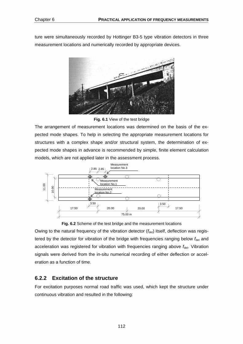
Chapter 6 PRACTICAL APPLICATION OF FREQUENCY MEASUREMENTS
112
ture were simultaneously recorded by Hottinger B3-5 type vibration detectors in three
measurement locations and numerically recorded by appropriate devices.
Fig. 6.1 View of the test bridge
The arrangement of measurement locations was determined on the basis of the ex-
pected mode shapes. To help in selecting the appropriate measurement locations for
structures with a complex shape and/or structural system, the determination of ex-
pected mode shapes in advance is recommended by simple, finite element calculation
models, which are not applied later in the assessment process.
Fig. 6.2 Scheme of the test bridge and the measurement locations
Owing to the natural frequency of the vibration detector (fdet) itself, deflection was regis-
tered by the detector for vibration of the bridge with frequencies ranging below fdet and
acceleration was registered for vibration with frequencies ranging above fdet. Vibration
signals were derived from the in-situ numerical recording of either deflection or accel-
eration as a function of time.
6.2.2 Excitation of the structure For excitation purposes normal road traffic was used, which kept the structure under
continuous vibration and resulted in the following:
2.85 2.85
11.0
0
10.0
0
75.00 m
3.503.50
20.00 20.00 17.50 17.50
Measurement location No.1
Measurement location No.2
Measurement location No.3
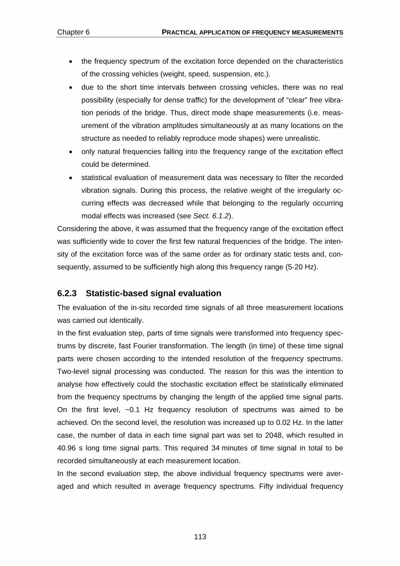
Chapter 6 PRACTICAL APPLICATION OF FREQUENCY MEASUREMENTS
113
• the frequency spectrum of the excitation force depended on the characteristics
of the crossing vehicles (weight, speed, suspension, etc.).
• due to the short time intervals between crossing vehicles, there was no real
possibility (especially for dense traffic) for the development of “clear” free vibra-
tion periods of the bridge. Thus, direct mode shape measurements (i.e. meas-
urement of the vibration amplitudes simultaneously at as many locations on the
structure as needed to reliably reproduce mode shapes) were unrealistic.
• only natural frequencies falling into the frequency range of the excitation effect
could be determined.
• statistical evaluation of measurement data was necessary to filter the recorded
vibration signals. During this process, the relative weight of the irregularly oc-
curring effects was decreased while that belonging to the regularly occurring
modal effects was increased (see Sect. 6.1.2).
Considering the above, it was assumed that the frequency range of the excitation effect
was sufficiently wide to cover the first few natural frequencies of the bridge. The inten-
sity of the excitation force was of the same order as for ordinary static tests and, con-
sequently, assumed to be sufficiently high along this frequency range (5-20 Hz).
6.2.3 Statistic-based signal evaluation The evaluation of the in-situ recorded time signals of all three measurement locations
was carried out identically.
In the first evaluation step, parts of time signals were transformed into frequency spec-
trums by discrete, fast Fourier transformation. The length (in time) of these time signal
parts were chosen according to the intended resolution of the frequency spectrums.
Two-level signal processing was conducted. The reason for this was the intention to
analyse how effectively could the stochastic excitation effect be statistically eliminated
from the frequency spectrums by changing the length of the applied time signal parts.
On the first level, ~0.1 Hz frequency resolution of spectrums was aimed to be
achieved. On the second level, the resolution was increased up to 0.02 Hz. In the latter
case, the number of data in each time signal part was set to 2048, which resulted in
40.96 s long time signal parts. This required 34 minutes of time signal in total to be
recorded simultaneously at each measurement location.
In the second evaluation step, the above individual frequency spectrums were aver-
aged and which resulted in average frequency spectrums. Fifty individual frequency

Chapter 6 PRACTICAL APPLICATION OF FREQUENCY MEASUREMENTS
114
spectrums were involved in the averaging process. By calculating these average spec-
trums:
• the relative weight of the stochastically occurring (excitation) frequencies de-
creased and that of the permanently present natural frequencies increased.
• if increasing the number of the individual frequency spectrums involved in the
averaging process, which required longer in-situ recorded time signals, the reli-
ability of natural frequencies read from the average frequency spectrum could
be improved. The reliability was measured by the standard deviation of fre-
quencies associated with the maximum ordinates in the individual spectrums.
0
5
10
15
20
25
30
35
40
0 1 2 3 4 5 6 7 8 9 10 11 12 13 14 15 16 17 18 19 20
Frequency [Hz]
Rel
ativ
e w
eigh
t
Measurement location No.1
Measurement location No.2
Measurement location No.3
7,8377,8377,837
9,2539,2539,253
13,96513,96513,965
16,57716,57716,577
Fig. 6.3 Average frequency spectrums of measurement locations
Fig. 6.3 shows that exactly the same numerical values for the first four natural frequen-
cies were obtained from the separate evaluation of signals recorded simultaneously at
the three measurement locations. The first natural frequency (f1), as the only available
modal data from previous investigations, was determined by field test as equal to 7.88
Hz in 1980 (Illéssy, 1980). Our measurement resulted in f1 very close to this value. No
information was available whether resurfacing, change of bearings or any structural
intervention was made during the elapsed period. Direct comparison of f1 values would
have been justified if information on these events were considered.
Since the ordinates of average frequency spectrums are of no sign, no information on
phase differences between the vibrating measurement locations could be obtained.
Thus, when using average spectrums, mode shapes associated with the natural fre-
quencies cannot be reproduced.

Chapter 6 PRACTICAL APPLICATION OF FREQUENCY MEASUREMENTS
115
6.2.4 Identification of mode shapes In order to make visible the phase differences between each two measurement loca-
tions during the vibration, the sum and the difference of recorded time signals belong-
ing to the considered two locations were composed. Then the average frequency spec-
trums of these “sum” and “difference” time signals were calculated (and noted by (1+2),
(1-2),…(2-3), respectively). For any two measurement locations, which vibrated in the
same phase in a mode, the “sum” time signal amplified the measured y(x) vibration
signal while the “difference” time signal minimized it. On the contrary, for other two
measurement locations, which vibrated in the opposite phase in a mode, the “sum”
time signal minimized the vibration sign while the “difference” signal amplified it. The
phase spectrums belonging to all possible measurement location pairs were obtained
by calculating the differences of the above average frequency spectrums composed
from the “sum” and “difference” time signals according to (Kálló, 1996). The amplitudes
in these phase spectrums, as shown in Fig. 6.4, had either positive or negative sign.
The sign of the amplitude at one of the natural frequencies indicated the phase differ-
ence between the considered two measurement locations in the mode associated with
the considered natural frequency. This made the reproduction of mode shapes associ-
ated with the already determined natural frequencies possible and, what is more impor-
tant, enabled them to be compared with the calculated mode shapes (see Sect. 6.2.1).
-60
-40
-20
0
20
40
60
1 2 3 4 5 6 7 8 9 10 11 12 13 14 15 16 17 18 19 20
Frequency [Hz]
Rel
ativ
e w
eigh
t
7,837
7,8377,837
9,2539,253
9,253
13,96513,965
13,965
16,57716,577
16,577
(1+2)-(1-2)
(1+3)-(1-3)
(2+3)-(2-3)
Fig. 6.4 Phase spectrums

Chapter 6 PRACTICAL APPLICATION OF FREQUENCY MEASUREMENTS
116
Based on the above sign rule, the phase spectrums in Fig. 6.4 suggested that the first
and the second mode were bending modes and that the fourth mode was a torsional
mode. The identification of the third mode, whose shape seemed to be a complex one,
was difficult. To clarify the shape of the third mode as well as the reason for the rela-
tively wide frequency range with uncertain peak in the spectrums between the second
and third natural frequency, computer models are helpful.

7 SUMMARY AND
NEW SCIENTIFIC RESULTS

Chapter 7 NEW SCIENTIFIC RESULTS
118
7.1 SUMMARY OF THE THESIS
This thesis deals with vibration-based, crack-related damage identification and
assessment of concrete model beams under experimental conditions.
The research was motivated by the fact that existing vibration-based damage
identification methods in the civil engineering field focus primarily on detection,
localization and maybe quantification of damage, but do not address structural
performance, which is of particular importance for owners to plan structural
interventions or to estimate remaining service life. The idea behind the research is that
any change in the modal data of a structure indicates a change in one or more of the
influencing parameters (mass, geometry, support conditions, stiffness, external forces).
If excluding intentional alteration of a structure and its operating conditions, damage-
caused changes in the influencing parameters can be revealed by dynamic
measurements during the service life.
This research was carried out on simply-supported beams, focused only on flexural
crack-related damage and used the first two natural frequencies and their shifts as
damage indicators. Damage was modelled either by cracking for reinforced concrete
beams or by the combination of cracking and tendon cuts for prestressed beams.
Damage was measured by the extent of cracking and by the extent of reduction in the
effective prestress due to tendon cuts. To model structural strengthening, post-
tensioning was applied to a few, already deteriorated reinforced concrete beams. To
reduce the effect of model uncertainties coming from modelling the structural behaviour
of cracked beams under vibration, damage assessment was carried out without the
development or use of dynamic models.
Chapter 1 gives a summary on damage identification in civil engineering by briefly
introducing existing vibration-based methods through a detailed literature review. A
comparison of methods is provided according to the information content of the
investigated parameter on the structure, practical applicability and sensitivity to
damage. Chapter 2 clarifies the concept and the goals of the research. Chapter 3
introduces the conducted laboratory test by describing the test beams, the execution of
the artificial deterioration process and the frequency measurements as well as the
applied signal processing and signal evaluation procedures. Chapter 4 defines,
classifies and determines calculated and measured damage indices used for crack-
related damage identification purposes. Chapter 5 establishes and concludes
relationships between the first two natural frequencies and the structural performance-
related parameters of test beams for assessment purposes. Chapter 6 demonstrates

Chapter 7 NEW SCIENTIFIC RESULTS
119
the practical applicability of frequency measurements with a simple test carried out on
a concrete highway bridge under service conditions.
7.2 PRACTICAL APPLICABILITY AND POSSIBLE FURTHER DEVELOPMENT OF THE RESEARCH
The introduced experimental, vibration-based damage identification and assessment
method consisted of a natural frequency measurement technique and a crack-related
damage assessment procedure. The measurement technique is available at low cost
for intermittent or continuous observation of natural frequencies of reinforced,
prestressed and post-tensioned concrete structures. Its application is mainly intended
for girder-type bridges, for which normal road traffic can be used for excitation
purposes. Using the relationships established between the measured natural
frequencies and the above performance-related parameters, any change in the
structural performance of the investigated structure during the service life can be
detected, localized and quantified on the basis of measured changes in the natural
frequencies.
Further development of the introduced method is possible in two main directions. The
first is the expansion of the range of measured dynamic characteristics in order to
increase the information content of on-site measurements on dynamic behaviour. This
is recommended only if the required effort (cost and time) of the on-site measurements
can be kept within reasonable limits. From this point of view, the inclusion of damping
parameters in this range is recommended. The second direction is either the further
improvement of the existing relationships between the measured dynamic
characteristics and the structural performance, or the definition of new ones. In this
area, the conducting of sensitivity studies, the provision of a statistical basis behind the
relationships as well as the extension of the concept of damage beyond flexural cracks
is desirable.
7.3 ACKNOWLEGEMENT
This work was connected to the scientific program of the “Development of quality-
oriented and harmonized R+D+I strategy and functional model at BME” project. This
project is supported by the New Hungary Development Plan (Project ID: TÁMOP-
4.2.1/B-09/1/KMR-2010-002).

Chapter 7 NEW SCIENTIFIC RESULTS
120
7.4 LIST OF THE NEW SCIENTIFIC RESULTS
The new scientific results of the presented work are summarized as follows.
New result 1 Based on a literature review, It was concluded that the existing dynamic-based damage
identification methods focus mainly on detection, localization and sometimes
quantification of damage but do not closely address structural performance-related
issues, which limits their practical applicability.
To overcome this, a new damage identification level (Level 3a) was defined. Beyond
damage identification, assessment methods fulfilling Level 3a are able to provide
information on the structural performance. It was pointed out that the effective practical
applicability of these methods requires:
a) the definition of performance-related damage indices that are based on
previous static models and able to identify damage as well as to measure its
extent (identification);
b) the establishment of relationships between the measured dynamic parameters
and the performance-related structural properties (assessment).
Related publications: [1],[3],[4],[5],[6],[7],[8],[9],[10],[14],[15],[17]
New result 2 Cracking-induced deterioration processes were modelled in experimental conditions on
simply supported, reinforced and prestressed concrete beams under flexure.
Meanwhile the first two natural frequencies of beams were determined at gradually
increasing damage levels. Damage was modelled by:
a) gradually intensified cracking due to defined, four-point mechanical loading for
the reinforced beams;
b) the combination of a) and artificially-made tendon cuts for the prestressed
beams;
c) the application of external post-tensioning (simulated strengthening effect) to a
few, already deteriorated reinforced concrete beams.
The extent of damage was measured by the extent of cracking and by the number of
tendon cuts. Alternatively, single mechanical impact and a periodic signal were used
for excitation purposes during the natural frequency measurements.
Related publications: [1],[3],[4],[5],[6],[7],[9],[10],[11],[12],[13],[14],[15],[17],[18]

Chapter 7 NEW SCIENTIFIC RESULTS
121
New result 3 A computational procedure for the evaluation of numerically-recorded acceleration-time
signals was developed. By the use of this, the first two natural frequencies of the test
beams were determined. The procedure was based on the statistical analysis of
discrete Fourier-transformed individual frequency spectrums. Using this technique, the
following were pointed out:
a) Both the average frequency spectrum (average spectrum method) and the average
value of frequencies associated with the maximum ordinate in the individual
spectrums (average frequency method) were solely able to indicate the first two
natural frequencies with an acceptably low (<1%) coefficient of variation for the
states of the beams in which the bending stiffness distribution remained symmetric
along the beam length.
b) For states where the bending stiffness distribution became non-symmetrical due to a
non-symmetrical crack pattern, multiple peaks occurred in the relevant frequency
spectrums. The value of the standard deviation associated with the average
frequency clearly indicated the presence of multiple peaks. If one of them was
dominant, then the combined use of the average spectrum method and the average
frequency method was required to estimate the true natural frequency as the
average of the frequencies associated with sub-peaks.
c) The first two natural frequencies could reliably (with a relative difference less than
1.5%) be determined from vibration signals derived from either impulse or periodic
excitation input, if no multiple peaks existed in the related frequency spectrums. If
multiple peaks existed, then the relative difference increased significantly (>>1.5%).
Related publications: [2],[6],[8],[16],[19]
New result 4 Static-based damage indices which reflected cracking-related damage and were in
accordance with a) of New result 1 were defined as follows:
• Growth of “total length of cracks”
• Growth of total and residual deflection at midspan
• Growth of crack width at midspan
• Growth of “total of crack sections”
• Growth of calculated midspan deflection
• Growth of calculated crack width at midspan
• Growth of internal strain energy

Chapter 7 NEW SCIENTIFIC RESULTS
122
Their values were determined for all deterioration states of the test beams. Their
classification was based on:
• their information content on the structure (global or local indices);
• the absence or the presence of any calculation model behind the index itself
and their involved parameters (non-model-based (measured) or model-based
(calculated)).
Depending on their intended purpose in damage identification, the indices were
interpreted in both incrementative (for detection purposes) and cumulative (for
quantification purposes) forms. Successful conformity checks were carried out between
the corresponding non-model-based and model-based indices.
Related publications: [1],[3],[4 ],[5],[6],[7],[9],[10],[11],[12],[13],[14],[15],[17],[18]
New result 5 By the use of the defined damage indices, damage identification as well as assessment
of test beams were carried out.
The defined indices were able to detect and to quantify the introduced artificial, crack-
induced damage in the beams. The identified damage was confirmed by the measured
natural frequency shifts.
Within the assessment, numerical relationships were established between the natural
frequency shifts and:
• for the reinforced concrete beams
− the internal force level;
− the extent of cracking immediately after the occurrence of first cracks;
− the type and amount of reinforcement;
• for the prestressed beams
− the internal force level;
− the extent of degradation in prestress;
• for the post-tensioned beams
− the intensity of the post-tensioning force.
Related publications: [5],[15],[17]

Chapter 7 NEW SCIENTIFIC RESULTS
123
New result 6 An in-situ frequency measurement and the respective signal evaluation were carried
out on an operational reinforced concrete highway bridge. The aim of the test was to
verify that reliable (with low standard deviation) determination of the first few natural
frequencies of the structure was possible under the service load of the bridge. For
excitation purposes the normal road traffic was used. The acceleration-time vibration
signals were recorded simultaneously in three measurement locations. It was found
that:
a) the excitation force of the normal road traffic was sufficiently high and smooth
over the target 5-20 Hz frequency range of the first four natural frequency of the
bridge. By the use of 34 min. long in-situ recorded acceleration-time signals at
each measurement location, this frequency range could be covered by discrete
Fourier transformed frequency spectrums with 0.02 Hz resolution;
b) the phase spectrums computed as combinations of average frequency
spectrums determined from sums and differences of acceleration-time signals
belonging to measurement locations of selected measurement location pairs
were capable of indicating the phase differences between the measurement
locations of the selected pairs in each mode. This made it possible to reproduce
the mode shapes associated with the measured natural frequencies.
Related publications: [2],[6],[8],[16],[19]

REFERENCES

REFERENCES
125
Publications referred in the main text of the dissertation (Sect. 1 – Sect. 6)
Aktan, A.E., Lee, K.L:, Chuntavan, C., Aksel, T., (1994) Modal testing for structural identification and condition assessment of constructed facilities, Proc. of the Int. Modal Analysis Conf., Honolulu, Hawaii, Vol.1, pp.462-468.
Alampalli, S., Fu, G., Dillon, E.W., (1997) Signal versus noise in damage detection by experimental modal analysis, Journal of Structural Engineering, Vol.123, No.2, pp.237-245.
Allemang, R.J., (2003) The Modal Assurance Criterion – twenty years of use and abuse, Sound and Vibration, August 2003, pp.14-21.
Andrade, C., (2003) Determination of chloride threshold in concrete, COST Action 521, Corrosion of steel in reinforced concrete structures, final report (eds.: R. Cigna, C. Andrade, U. Nürnberger, R. Polder, R. Weydert, E. Seitz), Part 2.4, European Commission, Directorate-General for Research, Brussels, Belgium, pp.101-111.
Armon, D., Ben-Haim, Y., Braun, S., Crack detection in beams by rank-ordering of eigenfrequency shifts, Mechanical Systems and Signal Processing, Vol.8, No.1, pp.81-91.
Bedics, A., Dubróvszky, G., Kovács, T., (2008) Development of the FI-150 precast concrete bridge girder family – design, production and application, Concrete Structures, Vol.9., Special issue for fib 2008 Amsterdam Symposium, Budapest, pp.2-9.
Begg, R.D., Mackenzie, A.C., Dodds, C.J., Loland, O., (1976) Structural integrity monitoring using digital processing of vibration signals, Proc. of the 8th Annual Offshore Technology Conference, Houston, TX, USA, pp.305-311.
Brincker, R., Anderson, P., Kirkegaard, P.H., Ulfkjaer, J.P., (1995a) Damage detection in laboratory concrete beams, Proc. of the 13th Int. Modal Analysis Conf., pp.668-674.
Brincker, R., Kirkegaard, P.H., Anderson, P., Martinez, M.E., (1995b) Damage detection in an offshore structure, Proc. of the 13th Int. Modal Analysis Conf., pp.661-667.
Casas, J.R., Aparicio, A.C. (1994) Structural damage identification from dynamic-test data, Journal of Structural Engineering, Vol.120, No.8, pp.2437-2450.
Catbas, F.N., Lenett, M.S., Aktan, A.E, Brown, D., Helmicki, A., Hunt, V., (1998) Damage detection and condition assessment of Seymour Bridge, Proc. of the 16th Modal Analysis Conference, Society of Experimental Mechanics, Bethel, Conn., USA, pp.381-389.
Catbas, F.N., Grimmelsman, K.A., Aktan, A.E., (2000) Structural identification of the Commodore Barry Bridge, Proc. of the SPIE’s 6th Int. Symposium on NDE and Health Monitoring and Diagnostics. Nondestructive evaluation of Highways, Utilities and Pipelines (eds.: A.E. Aktan and S.R. Gosselin), Int. Society for Optical Engineering, Bellingham, Washington, USA, Vol.3995, pp.84-97.
REFERENCES
126
Catbas, F.N., Aktan, A.E., (2002) Condition and damage assessment: Issues and some promising indices, Journal of Structural Engineering, Vol.128, No.8, pp.1026-1036.
Cawley, P., Adams, R.D., (1979) The location of defects in structures from measurements of natural frequencies, Journal of Strain Analysis, Vol.14, No.2, pp.49-57.
Chan, T., Ko, J.M., Lau, C.K., Wong, K.Y., (1998) Vibration measurement of Tsing Ma Bridge deck units during erection, Long-Span and High-Rise Structures, IABSE Symposium Report, Kobe, Japan, Vol.79, pp.275-280.
Chase, S.B., Laman, J.A., (2000) Dynamics and field testing of bridges, Tansportation in the New Millennium, http://www.nacionalacademies.org/trb/publications/millennium/00029.pdf
Choy, F.K., Liang, R., Xu, P., (1995) Fault identification of beams on elastic foundation, Computers and Geotechnics, Vol.17, pp.157-176.
Coppolino, R.N., Rubin, S., (1980) Detectability of structural failures in offshore platforms by ambient vibration monitoring, Proc. of the 12th Annual Offshore Technology Conference, pp.101-110.
COST Action 521, (2003) Corrosion of steel in reinforced concrete structures, final report (eds.: R. Cigna, C. Andrade, U. Nürnberger, R. Polder, R. Weydert, E. Seitz), European Commission, Directorate-General for Research, Brussels, Belgium
Curadelli, R.O., Riera, L.D., Ambrosini, D., Amani, M.G. (2008) Damage detection by means of structural damping identification, Engineering Structures, Vol.30, pp.3497-3504.
Della Vedova, M., Evangelista, L. (2004) Protection against corrosion and monitoring of post-tensioning tendons in prestressed concrete railway bridges in Italy, 1st Workshop of COST 534, NDT assessment and new systems in prestressed concrete structures, Zurich, Switzerland, pp.77-84.
Doebling, S.W., Hemez, F.M., Peterson, L.D., Farhat, C. (1997a) Improved damage location accuracy using strain energy-based mode selection criteria, J22609, Los Alamos National Laboratory, Los Alamos, NM, USA
Doebling, S.W., Farrar, C.R., Goodman, R.S., (1997b) Effects of measurement statistics on the detection of damage in the Alamosa Canyon Bridge, Proc. of the 15th Int. Modal Analysis Conference, Orlado, FL, USA, pp.919-929.
Doebling, S.W., Farrar, C.R., Prime, M.B., Shevitz, D.W., (1996) Damage identification and health monitoring of structural and mechanical systems from changes in their vibration characteristics: A literature review, LA-13070-MS, Los Alamos National Laboratory, Los Alamos, NM, USA
Doebling, S.W., Farrar, C.R., Prime, M.B., (1998) A summary review of vibration-based damage identification methods, The Shock and Vibration Digest, Vol.30, No.2, pp.91-105.

REFERENCES
127
Dong C., P.Q. Zhang, W.Q. Feng, T.C. Huang, (1994) The sensitivity study of the modal parameters of a cracked beam, Proc. of the 12th Int. Modal Analysis Conference, pp.98-104.
Ebert, M., (2001) Experimental and numerical investigation of the dynamic behaviour of reinforced concrete structures taking into account stochastic material properties, PhD dissertation, Weimar, Germany (in German)
Elsener, B. (2004a) Electrical isolation as enhanced protection for post-tensioning tendons in concrete structures (PL3), 1st Workshop of COST 534, NDT assessment and new systems in prestressed concrete structures, Zurich, Switzerland, pp.71-76.
Elsener, B. (2004b) Experience with electrically isolated tendon in Switzerland, 1st Workshop of COST 534, NDT assessment and new systems in prestressed concrete structures, Zurich, Switzerland, pp.85-93.
EN 206-1:2000, Concrete - Part 1: Specification performance, production and conformity, CEN, Brussels, Belgium
EN 1990:2002, Eurocode - Basis of structural design, CEN, Brussels, Belgium
EN 1992-1-1:2004, Eurocode 2: Design of concrete structures - Part 1-1: General rules and rules for buildings, CEN, Brussels, Belgium
Enright, M.P., Frangpool, D.M., (1999) Reliability-based condition assessment of deteriorating concrete bridges considering load redistribution, Structural safety, Vol.21, No.2, pp.159-195.
Enright, M.P., Frangpool, D.M., (2000) Reliability based lifetime maintenance of aging highway bridges, Proc. of the SPIE’s 6th Int. Symposium on NDE and Health Monitoring and Diagnostics. Nondestructive evaluation of Highways, Utilities and Pipelines (eds.: A.E. Aktan and S.R. Gosselin), Int. Society for Optical Engineering, Bellingham, Washington, USA, Vol.3995, pp.4-13.
Farkas, Gy., (1998) Supervision, maintenance and renovation of reinforced and prestressed concrete bridges, Extended abstracts of the SMART-98 NATO Advanced Research Workshop (ed.: J. Holnicki-Szulc), Pultusk, Poland, pp.39-42.
Farkas, Gy., Szalai, K., (1998) Supervision of the Bodrog Bridge at Alsóberecki, Közúti Közlekedés és Mélyépítéstudományi Szemle, Vol.XLVIII., No.4.
Farrar, C.R., Doebling, S.W., Cornwell, P.J., Straser, E.G., (1997) Variability of modal parameters measured on the Alamosa Canyon Bridge, Proc. of the 15th Int. Modal Analysis Conference, Orlado, FL, USA, pp.257-263.
Farrar, C.R., Doebling, S.W., Duffey, T.A., (1999) Vibration-based damage detection, presented at the SD 2000 Structural Dynamics Forum, April 11-17, 1999.
Farrar, C.R., Jauregui, D.A. (1998) Comparative study of damage identification algorithms applied to a bridge: I. Experiment, Smart Materials and Structures, Vol.7, pp.704-719.
fib Bulletin No. 34, (2006) Model Code for Service Life Design, fib TG 5.6

REFERENCES
128
Forde, M.C. (2004) Sonic & ultrasonic NDT methods in the assessment of concrete structures, 1st Workshop of COST 534, NDT assessment and new systems in prestressed concrete structures, Zurich, Switzerland, pp.55-70.
Fujino, Y., Abe, M., (2001) Structural health monitoring in civil infrastructures and R&D of SHM of bridges at University of Tokyo, Proc. of the 3rd Int. Workshop on Structural Health Monitoring: The Demands and Challenges, Stanford, CA, USA, pp.61-79.
Goble G., Schulz, J., Commander, B., (1992) Load prediction and structural response, Final Report, FHWA DTFH61-88-C-00053, University of Colorado, Boulder, Colorado, USA
Golaski, L., (2004) Acoustic emission monitoring of reinforced concrete elements an overview, 1st Workshop of COST 534, NDT assessment and new systems in prestressed concrete structures, Zurich, Switzerland, pp.7-24.
Harichandran, R., Hong, S., (2003) Sensors to monitor bond in concrete bridges rehabilitated with FRP, Final report, Dept. of Civil and Environmental Engineering, Michigan State University, MI, USA
Hearn, G., Testa, R.B., (1991) Modal analysis for damage detection in structures, Journal of Structural Engineering, Vol.117, No.10, pp.3042-3063.
Hemez, F.M., Farhat, C. (1995) Structural damage detection via a finite element model updating methodology, Modal Analysis: The Int. Jounal of Analytical and Experimental Modal Analysis, Vol.3, No.3, pp.152-166.
Hillemeier, B., Scheel, H. (2004) Location of prestressing wire breaks with the remanent magnetism method, 2st Workshop on Durability of post tensioned tendons, Zurich, Switzerland, pp.139-152.
Huszár, Zs., (2009) Vibration analysis of continuum-modelled structures, PhD értekezés, Dept. of Structural Engineering, Budapest University of Technology and Economics, Budapest, Hungary
Illéssy, J., (1977) Structural stiffnesses of RC constructions: Their determination by non-destructive site investigations and use of the actual values, Testing in situ, RILEM, 1977/I, pp.283-294.
Illéssy, J., (1980) On the non-destructive testing possibilities of ageing bridges, Study, No.21.552/80, Institute for building research, Budapest, Hungary,
Illéssy, J., (1982) On the investigation for condition by easily reproducible dynamic “in-situ” short-time measurements to establish lifetime prognoses of structures, Manuscript for the 9th Int. Congress of the FIP, Stockholm, Institute for Building Sciences, Budapest, Hungary
IMT poject: BRPR-CT95-0099 (2003). Quality assessment of grouting. Task 2.0: Sensos as an aid to quality assessment and quality control of grouting, Freyssinet Co.
Ismail, F., Ibrahim, A., Martin, H.R., (1990) Identification of fatigue cracks from vibration testing, Journal of Sound and Vibration, Vol.140, pp.305-317.

REFERENCES
129
Kato, M., Shimada, S., (1986) Vibration of PC bridge during failure process, Journal of Structural Engineering, Vol.112, No.7, pp.1692-1703.
Kálló, M, (1996) Simple measuring procedure to determine natural frequencies and mode shapes of bridges. Dynamic bride tests, Proc. of the scientific workshop, Győr, 2. paper
Kálló, M. (1997) Quasi-modal analysis using quasistochastic signals of bridges, Österreichische Ingenieur- und Architekten- Zeitschrift (ÖIAZ), Vol.142, No.5. pp.391-396.
Kenley, R.M., Dodds, C.J., (1980) West Sole WE Platform: Detection of damage by structural response measurements, Proc. of the 12th Annual Offshore Technology Conference, pp.111-118.
Koh, C.G., See, L.M., Balendra, T., (1995) Damage detection of buildings: numerical and experimental studies, Journal of Structural Engineering, Vol.121., No.8, pp.1155-1160.
Korany, Y., Rizkalla, S., (2000) Taylor Bridge – The New generation, The University of Manitoba & ISIS Canada, Winnipeg, Manitoba, Canada
Kovács, T., (1998a) Dynamic investigations on reinforced concrete bridges, Proc. of the 2nd Int. PhD Symposium in Civil Engineering (ed: Balázs L.Gy.), Műegyetemi Kiadó, Budapest, Hungary, pp. 197-204.
Kovács, T., Farkas, Gy., Kálló, M., (1998b) Investigation of dynamic characteristics for concrete bridges, Scientific Publications of the Dept. of Reinforced Concrete Structures, Budapest Univ. of Technology and Economics (eds: Tassi, G., Kovács T.), Műegyetemi Kiadó, Budapest, Hungary, pp.111-124.
Kovács, T., Farkas, Gy., (2000) The assessment of damage by dynamic characteristics on model beams, Proc. of the 3rd Int. PhD Symposium in Civil Engineering (ed: K. Bergmeister), Vienna, Austria, Vol.1, pp. 297-306.
Lenett, M.S., Griessman, A., Helmicki, A.J., Aktan, A.E. (1999) Subjective and objective evaluations of bridge damage, Journal of Transportation Research Board, 1688, pp.76-86.
Lim, T.W. (1995) Structural damage detection using constrained eigenstructure assignment, Journal of Guidance, Control and Dynamics, Vol.18, No.3, pp.411-418.
Lin, C.S. (1994) Unity check method for structural damage detection, Proc. of the 35th AIAA/ASME/ASCE/AHS/ASC structures, Structural Dynamics and Materials Conf., AIAA-94-1717-CP, pp.347-354.
Lin, R.M., Ewins, D.J. (1990) On the location of structural nonlinearity from modal testing - A feasibility study, Proc. of the 8th Int. Modal Analysis Conf., pp.358-364.
Maeck, J., (2003) Damage assessment of civil engineering structures by vibration monitoring, PhD dissertation, Div. of Structural Mechanics, Dept. of Civil Engineering, Catholic University of Leuven, Leuven, The Netherlands

REFERENCES
130
Mazurek, D.F., DeWolf, J.T., (1990) Experimental study of bridge monitoring technique, Journal of Structural Engineering, Vol.116, No.9, pp.2532-2549.
Messina, A., Jones, I.A., Williams, E.J., (1996) Damage detection and localisation using natural frequency changes, Proc. of the Conf. on Identification in Engineering Systems, Swansea, United Kingdom, pp.67-76.
Messina, A., Williams, E.J., Contursi, T., (1998) Structural damage detection by a sensitivity and statistical-based method, Journal of Sound and Vibration, Vol.216, No.5, pp.791-808.
Miyagawa, T., Nojima, S., Tokumitsu, S., Hosono, H., Tezuka, M. (2004) Present situation of maintenance, assessment and rehabilitation in Japan, 2st Workshop on Durability of post tensioned tendons, Zurich, Switzerland, pp.123-138.
Morassi, A., (2001) Identification of a crack in a rod based on changes in a pair of natural frequencies, Journal of Sound and Vibration, Vol.242, No.4, pp.557-596.
Mutsuyoshi, H., Hamada, Y., Igo, Y., Watanabe, H., (2004) Design concepts for durable prestressed concrete structures in Japan, 2nd Workshop on Durability of post-tensioning tendons (ed.: B. Elsener), Zurich, Switzerland, pp.13-22.
Narkis, Y., (1994) Identification of crack location in vibrating simply supported beams, Journal of Sound and Vibration, Vol.172, No.4, pp.549-558.
Pandey, A:K., Biswas, M., Samman, M.M. (1991) Damage detection from changes in curvature mode shapes, Journal of Sound and Vibration, Vol.145, No.2, pp.321-332.
Pandey, A.K., Biswas, M. (1994) Damage detection in structures using changes in flexibility, Journal of Sound and Vibration, Vol.169, No.1, pp.3-17.
Pandey, A.K., Biswas, M. (1995) Experimental verification of flexibility difference method for locating damage in structures, Journal of Sound and Vibration, Vol.184, No.2, pp.311-328.
Penny, J.E.T., Wilson, D.A.L., Friswell, M.I., (1993) Damage location in structures using vibration data, Proc. of the 11th Int. Modal Analysis Conf., Kissimmee, FL, USA, pp.861-867.
Poston, R.W., West, J.S. (2004) North American strategies for monitoring, maintenance and repair of post-tensioning tendons, 2st Workshop on Durability of post tensioned tendons, Zurich, Switzerland, pp.103-122.
Raghavendrachar, M., Aktan, A.E., (1992) Flexibility by multireference impact testing for bridge diagnostics, Journal of Structural Engineering, Vol.118, No.8, pp.2186-2203.
Ratcliffe, C.P., (1997) Damage detection using a modified Laplacian operatot on mode shape data, Journal of Sound and Vibration, Vol.204, No.3, pp.505-517.
Richardson, M.H., Mannan, M.A., (1992) Remote detection and location of structural faults using modal parameters, Proc. of the 10th Int. Modal Analysis Conference, pp.502-507.
REFERENCES
131
Rizos, P.F., Aspragathos, N., Dimarogonas, A.D., (1990) Identification of crack location and magnitude in a cantilever beam from the vibration modes, Journal of Sound and Vibration, Vol.138, No.3, pp.381-388.
Rytter, A., (1993) Vibration based inspection of civil engineering structures, PhD dissertation, Dept. of Building Technology and Structural Engineering, Aalborg University, Denmark
Salane, H.J., Baldwin, J.W. (1990) Identification of modal properties of bridges, Journal of Structural Engineering, Vol.116, No.7, pp.2008-2021.
Salawu, O.S., (1997a) Detection of structural damage through changes in frequency: a review, Engineering Structures, Vol.19, No.9, pp.718-723.
Salawu, O.S., (1997b) An integrity index method for structural assessment of engineering structures using modal testing, Insight, Vol.39, No.1, pp.33-37.
Salawu, O.S., Williams, C., (1994) Damage location using vibration mode shapes, Proc. of the 12th Int. Modal Analysis Conference, pp.933-939.
Salawu, O.S., Williams, C., (1995) Bridge assessment using forced-vibration testing, Journal of Structural Engineering, Vol.121, No.2, pp.161-173.
Schickert, G., (1997) NDT-CE symposium Berlin 1995: A concluding review, NDTnet, Vol.2, No.04
Schulz, W.L., Udd, E., Seim, J.M., McGill, G.E. (1998) Advanced fiber grating strain sensor systems for bridges, structures and highways, Proc. of the SPIE’s Int. Symposium on NDE and Health Monitoring and Diagnostics. Nondestructive evaluation of Highways, Utilities and Pipelines, Int. Society for Optical Engineering, Bellingham, Wash., Vol.3325, pp. 212-222.
Shi, Z.Y., Law, S.S., Zhang, L.M (1998) Structural damage localization from modal strain energy strange, Journal of Sound and Vibration, Vol.218, No.5, pp.825-844.
Shi, Z.Y., Law, S.S., Zhang, L.M (2000) Structural damage detection from modal strain energy strange, Journal of Engineering Mechanics, Vol.126, No.12, pp.1216-1223.
Sohn, H., Farrar, C.R., Hemez, F.M., Czarnecki, J.J., Shunk, D.D., Stinemates, D.W., Nadler, B.R., (2003) A review of structural health monitoring literature: 1996-2001, LA-13976-MS, Los Alamos National Laboratory, NM, USA
Strukelj, A., Ciglaric, I., Pipenbaher, M., (2005) Analysis of a bridge structure and its wind barrier under wind loads, Structural Engineering International, Vol.4, pp.220-227.
Stubbs, N., Osegueda, R., (1990a) Global non-destructive damage evaluation in solids, Modal Analysis: The Int. Journal of Analytical and Experimental Modal Analysis, Vol.5, No.2, pp.67-79.
Stubbs, N., Osegueda, R., (1990b) Global damage detection in solids – experimental verification, Modal Analysis: The Int. Journal of Analytical and Experimental Modal Analysis, Vol.5, No.2, pp.81-97.
REFERENCES
132
Stubbs, N., J.-T. Kim, K. Topole, (1992) An efficient and robust algorithm for damage localization in offshore platforms, Proc. of the ASCE Tenth Structures Congress, pp.543-546.
Topole, K.G, Stubbs, N. (1995) Non-destructive damage evaluation of a structure from limited modal parameters, Earthquake Engineering and Structural Dynamics, Vol.24, No.11, pp.1427-1436.
Waalkes, S.M., (2003) Life-cycle cost analysis: A guide for comparing alternate pavement designs, American Concrete Pavement Association, Skokie, Illinois, USA, EB220, p.49.
Watson, J.R., (2004) Advanced acoustic emission monitoring of concrete structures, 1st Workshop of COST 534, NDT assessment and new systems in prestressed concrete structures, Zurich, Switzerland, pp.31-43.
Wenzel, H., Pichler, D., Geier, R., (2003) BRIMOS® Bridge Monitoring System, Dynamic system identification and damage detections in bridge structures, Examination and assessment of structures in practice, Proc. of the SAMCO 2003, Cambridge, UK
de Wit, M., (2004) The use of acoustic monitoring to manage concrete structures, 1st Workshop of COST 534, NDT assessment and new systems in prestressed concrete structures, Zurich, Switzerland, pp.25-30.
Yuen, M.M.F., (1985) A numerical study of the eigenparameters of a damaged cantilever, Journal of Sound and Vibration, Vol.130, No.3, pp.301-310.
Zhang, Z., Aktan, A:E. (1995) The damage indices for constructed facilities, Proc. of the 13th Int. Modal Analysis Conference, pp.1520-1529.
Zimmermann, D.C., Smith, S.W., (1992) Model refinement and damage location for intelligent structures, Intelligent Structural Systems (ed. H.S. Tzou and G.L. Anderson), Kluwer Academic, pp.403-452.
Zonta, D., Elgamal, A., Fraser, M., Priestley, M.J.N. (2008) Analysis of change in dynamic properties of a frame-resistant test building, Engineering Structures, Vol.30, pp.183-196.
REFERENCES
133
Publications referred in the new scientific results (Sect. 7)
Book, sections in book [1] Kovács, T. – Farkas, Gy.: Condition monitoring of reinforced concrete beams by dynamic
measurements, Sec. 3.5.4. in book entitled as New Materials, systems, methods and concepts for prestressed concrete structures, final report of COST 534, Eds: R.B. Polder, M.C. Alonso, D.J. Cleland, B. Elsener, E. Proverbio, Ø. Vennesland, A. Raharinaivo, Cost Office, 2009, ISBN 9789059863323, pp. 192-194.
Paper in collected volume [2] Kovács T. - Farkas Gy. – Kálló M.: Vasbeton hidak dinamikus jellemzőinek vizsgálata, BME
Vasbetonszerkezetek Tanszéke Tudományos Közleményei (szerk.: Tassi G., Kovács T.), 1998., Műegyetemi Kiadó, Budapest, pp. 111-124.
[3] Kovács T. − Farkas Gy.: Károsodásbecslés dinamikai jellemzők alapján, BME Hidak és Szerkezetek Tanszéke Tudományos Közleményei (szerk.: Tassi G., Hegedűs I., Kovács T.), 2001., Műegyetemi Kiadó, Budapest, pp. 125-138.
[4] Kovács, T. – Farkas, Gy.: Damage assessment by frequency measurements on reinforced concrete beams, Workshop of COST on „NDT Assessment and New Systems in Prestressed Concrete Structures”, COSt Action 534, Institute for Terotechnology – NRI, Kielce, Poland, September 19-21, 2005. pp. 201-216.
[5] Kovács, T.: Natural frequency shifts for concrete beams due to deterioration-induced cracks, Scientific publicatons of the Dept. of Structural Engineering, (ed.: Tassi, G., Hegedűs, I., Kovács, T.), 2009., Műegyetemi Kiadó, Budapest, pp. 115-122.
International journal paper [6] Kovács, T. − Farkas, Gy.: Effect of cracking on the dynamic characteristics of concrete
beams, Concrete Structures, Vol.3, Special issue for fib 2002 Osaka Congress, 2002, Budapest, pp. 64-69.
Domestic journal paper in English [7] Kovács, T. – Farkas, Gy.: Condition monitoring of a lightly reinforced concrete beam by
dynamic measurements, Periodica Politechnika Ser. Civ. Eng., Vol.49, No.1, 2005. pp. 27-46.
International conference paper [8] Kovács, T.: Dynamic investigations on reinforced concrete bridges, Proc. of the 2nd
International PhD Symposium in Civil Engineering, Budapest, 26-28 August 1998, pp. 197-204.
[9] Kovács, T. – Farkas, Gy.: The assessment of damage by dynamic characteristics on model beams, Proc. of the 3rd International PhD Symposium in Civil Engineering, Vienna, 5-7 October 2000, Volume 1, pp. 297-306.
[10] Farkas, Gy. − Kovács, T.: The assessment of damage by dynamic characteristics, 3rd Korean-Hungarian Symposium on “New methods in structural engineering” (organizer: Hungarian Academy of Engineering), Budapest, June 22, 2001.
[11] Farkas, Gy. − Kovács T.: The assessment of damage by dynamic characteristics, 4th International Conference on Bridges Across the Danube, Bratislava, Slovakia, September 13-15 2001, pp. 217-222.
[12] Kovács, T.: The effects of cracking on the natural frequencies for concrete beams, Proc. of the 4th International PhD Symposium in Civil Engineering, Munich, 19-21 September 2002, Volume 1, pp. 338-344.
[13] Kovács, T. – Farkas, Gy.: Condition monitoring of concrete beams by dynamic measurements, Proc. of the IABSE Symposium on „Responding to tomorrow’s challenges

REFERENCES
134
in structural engineering”, Budapest, Hungary, September 13-15 2006, pp. 112-113, CD-ROM
[14] Kovács, T. – Farkas, Gy.: Damage assessment by dynamic measurements on concrete bridges, Proc. of the International Conference on Bridges, Dubrovnik, Croatia, May 21-24 2006, pp. 1067-1074.
[15] Kovács, T.: Influence of deterioration on the dynamic behaviour of concrete beams, Proc. of the fib Symposium on Concrete: 21st century superhero + CD ROM, London, UK, June 22-24, 2009, 8 pages
[16] Kovács, T.: In-situ dynamic measurements on a concrete bridge, Proc. of the 5th Central European Congress on Concrete Engineering on „Concrete engineering in urban development”, Baden, Austria, September 24-25, 2009, pp. 306-310.
[17] Kovacs, T.: Effect of deterioration-induced cracks on the modal properties of concrete beams, Proc. disk of The Third Int. Congress and Exhibition „Think globally, Build Locally”, ID 628, Washington, USA, May 29-June 2, 2010, 9 pages
Hungarian conference paper [18] Kovács T. – Farkas Gy.: Károsodásbecslés dinamikai jellemzőkkel, Műszaki Mechanika
2002., MTA-BME Mechanikai Kutatóközösség VII. Tudományos Ülésszaka, Budapest, 2001. január 30., Műegyetemi Kiadó, pp. 61-66.
Technical Report [19] Farkas, Gy. – Hegedűs, I. – Koris, K. – Kovács, T.: Final Scientific Report by The Dept.
of Reinforced Concrete Structures, Budapest Univ. of Techn. and Economics, COPERNICUS Joint Project: "Innovative Simulation Tools for the Durability-Design and Maintenance-Management of Reinforced Concrete Traffic Infrastructure", Contract Number IC15-CT96-0755, Budapest, March 10., 2000.

APPENDIX
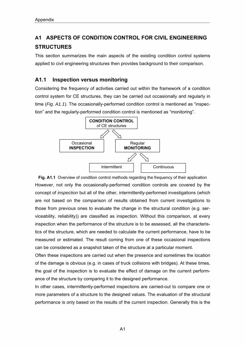
Appendix
A1
A1 ASPECTS OF CONDITION CONTROL FOR CIVIL ENGINEERING STRUCTURES This section summarizes the main aspects of the existing condition control systems
applied to civil engineering structures then provides background to their comparison.
A1.1 Inspection versus monitoring Considering the frequency of activities carried out within the framework of a condition
control system for CE structures, they can be carried out occasionally and regularly in
time (Fig. A1.1). The occasionally-performed condition control is mentioned as “inspec-
tion” and the regularly-performed condition control is mentioned as “monitoring”.
Fig. A1.1 Overview of condition control methods regarding the frequency of their application
However, not only the occasionally-performed condition controls are covered by the
concept of inspection but all of the other, intermittently-performed investigations (which
are not based on the comparison of results obtained from current investigations to
those from previous ones to evaluate the change in the structural condition (e.g. ser-
viceability, reliability)) are classified as inspection. Without this comparison, at every
inspection when the performance of the structure is to be assessed, all the characteris-
tics of the structure, which are needed to calculate the current performance, have to be
measured or estimated. The result coming from one of these occasional inspections
can be considered as a snapshot taken of the structure at a particular moment.
Often these inspections are carried out when the presence and sometimes the location
of the damage is obvious (e.g. in cases of truck collisions with bridges). At these times,
the goal of the inspection is to evaluate the effect of damage on the current perform-
ance of the structure by comparing it to the designed performance.
In other cases, intermittently-performed inspections are carried-out to compare one or
more parameters of a structure to the designed values. The evaluation of the structural
performance is only based on the results of the current inspection. Generally this is the
CONDITION CONTROL of CE structures
Occasional INSPECTION
Regular MONITORING
Intermittent Continuous

Appendix
A2
case for bridges in many countries, for instance in Hungary, when the responsible
bridge authority is officially obliged to carry out inspections on bridges after every given
period - depending on the importance of the bridge - in order to verify the adequate
reliability of their structures. At these inspections, if no obvious damage is known, gen-
erally the deflections of the structure are measured in typical points due to appropri-
ately positioned static trucks (static load test, see Sect. A1.3.2) and compared to the
corresponding calculated values.
Without the mentioned comparison and without any more sophisticated damage detec-
tor and localizing technique, these simple inspections are not able to detect and to lo-
calize hidden damage in CE structures.
If the condition control activities are performed regularly and based on the comparison
of the current measurements or their results to those of the previous investigations, a
monitoring process is occurring. Naturally, in most cases, an assessment method sup-
plements the monitoring process, by which the system is capable of damage localiza-
tion as well as structural condition evaluation.
A monitoring process can be carried out continuously in time by the application of on-
line measuring techniques using different kinds of sensors and/or videos, which are
either embedded in the (concrete) structure or externally fixed to it (Harichandran and
Hong, 2003). When using sensors, either an electronic or a wireless communication
system is necessarily installed between the sensors and the data acquisition instru-
ment (Schulz et al.,1998).
The 165.1 m long Taylor Bridge (1997), which spans the Assiniboine River in Canada
and is fully made of prestressed concrete with fibre reinforced polymers as reinforce-
ment, is equipped with 66 fibre optic sensors coupled with conventional embedded
electric strain gauges, which communicate with the engineers through telephone lines
(Korany and Rizkalla, 2000). The Tsing Ma Bridge (1997), which crosses the 1377 m
wide Ma Wan Channel in Hong Kong, is equipped with 600 sensors to monitor the
structure permanently (Farrar et al., 1999; Chan et al., 1998) (Fig. A1.2).
Taylor Bridge, Winnipeg, Canada Tsing Ma Bridge, Hong Kong, China
Fig. A1.2 “Smart” bridges equipped with continuous monitoring systems

Appendix
A3
The earliest monitoring systems work intermittently rather than continuously in time.
These are not capable of on-line data transfer however the essence of operation is
similar to those for the continuously working systems. The measurements are usually
repeated daily, weekly, monthly or yearly depending on the needs of the owner or the
engineers.
A1.2 Diagnostic techniques The diagnostic (inspection/monitoring) techniques can be categorized as local or global
techniques (Fig. A1.3).
Fig. A1.3 Local and global diagnostic techniques
A1.2.1 Local diagnostic techniques In this context, a local technique is considered as a group of activities which focuses on
the affected structural part(s) only and detects damage by often measuring the change
in a particular quantity. Based on this change, the method is able to detect and some-
times characterize the severity of the damage. The selection of the measured quantity
DIAGNOSTIC techniques
LOCAL techniques
GLOBAL techniques
Non-instrumental technique Visual inspection
Instrumental techniques Ultrasonic pulse velocity Ultrasonic pulse-echo Acoustic emission Electrical and electro-chemical methods Interferometry Impact-echo Magnetic methods Microwaves Radar Infrared thermography Laser applications Radiography, radiometry Computer tomography Nuclear Magnetic Resonance Time domain reflectometry Electro-acoustical methods Ultrasonic resonance spec-troscopy Gas permeability Heat transmission Optical methods
Static load test (and analysis) Moving load test (and analy-sis) Vibration test (and modal analysis)

Appendix
A4
depends on the applied measurement technique. It means that the vicinity of damage
to be quantified has to be known beforehand, otherwise a full scan trough the whole
structure is needed to detect damage first. The crucial point is that a local diagnostic
technique does not take into account the global behaviour (response) of the structure in
the structural evaluation even if it is:
repeated as many times per investigation as needed to perform a full scan
through the entire structure and
used for regularly scanning (monitoring) the structure.
The local diagnostic techniques can be classified as non-instrumental or instrumental
techniques.
The only obvious non-instrumental technique is the visual inspection. It is heuristic and
fully based on the experience and the knowledge of the applying person. There is a
lack of close correlation between visual appearance and structural reliability of a struc-
ture. Visual inspections find signs of corrosion and damage such as cracks, spalls, lo-
cal brittle failures, chemical attacks, etc. only when those become visible. The influence
of damage on the structural reliability, which can be considerably different for steel or
concrete structures, is very difficult to establish based on these inspections. The
causes of the observed damage can also not be clearly identified. Thus, the judgement
of the structure is also based mainly on experience.
Based on Schickert (1997), Fig. A1.3 lists the most frequently applied, instrumental
local damage detecting techniques in the sequence of their usefulness in the civil engi-
neering field. The developed techniques and their applied methods are generally used
to measure different properties of material such as strength, thickness, water content,
moisture content, density, porosity, thermal conductivity, permeability, surface proper-
ties, etc. and, in several cases, those of structural parts such as cracking, fractures,
integrity, delamination, presence of air and liquid voids, holes or hidden objects, posi-
tion of reinforcement, corrosion activity (carbonation, chloride-attack), stress intensity,
etc. Similar review on the instrumental local damage detecting techniques for grouting
of prestressing tendons is included in IMT (2003).
A complete COST action (COST Action 521) dealt with the corrosion and the corrosion
monitoring of steel embedded in concrete (COST, 2003) by local techniques. It particu-
larly focused on the corrosion state monitoring of reinforcing steel by using embedded
sensors and electrochemical techniques, determining the chloride threshold as well as
on particular maintenance methods (electrochemical methods, surface applied inhibi-
tors, surface treatments and coatings, durability of patch repairs). The COST Action

Appendix
A5
534 (New Materials and Systems for Prestressed Concrete Structures) mainly focused
on the non-destructive monitoring of prestressed concrete structures with the use of
acoustic emission techniques (Golaski, 2004; de Wit, 2004; Watson, 2004), ultrasonic
methods (Forde, 2004) and electrical isolation (Elsener, 2004a, 2004b; Vedova and
Evangelista, 2004). Magnetic methods are also frequently used to locate prestressing
tendon breaks in different types of prestressed concrete structures including bridge
decks and parking structures (Hillemeier and Scheel, 2004). Significant efforts are
made in many countries to develop and improve techniques as well as testing methods
to detect and locate local damage in post-tensioning tendons (Poston and West, 2004;
Miyagawa et al., 2004).
It is important to see from the literature that the above instrumental local techniques are
being apparently used more and more frequently in practice for monitoring purposes
rather than as a damage locating tool for occasionally-performed state controls. These
techniques involve significant cost and, in spite of this, the current performance (reli-
ability) and the remaining service life (Level 4) of the whole structure, which are very
meaningful pieces of information for both the owner and the engineers, can not be as-
sessed on the basis of these investigations.
A1.2.2 Global diagnostic techniques (methods) Based on the foregoing, a global diagnostic method is considered if the global behav-
iour of the structure is measured in-situ in an appropriate way and the structural (condi-
tion) evaluation (damage assessment) is based on these results. The key issue is the
recording and the consideration of the response of the whole structure influenced by
deterioration. This makes it possible to define deterioration mechanisms, to make dis-
tinctions between different damage with respect to their risk and to clearly understand
how local damage affects the performance of the whole structure.
In using a global technique, the location of a possible deficiency does not need to be
known beforehand. Since global diagnostic methods record the response of the whole
structure at given points rather than performing local scans around the damage-
affected structural part, they have to be supplemented by evaluation algorithms or
postprocessing tools, which transform the recorded data into meaningful quantities,
diagrams, graphs, etc., which more comprehensively and visibly show the structural
performance for both the engineers and the owner. Fig. A1.3 lists the most frequently
used global diagnostic techniques (Catbas and Aktan, 2002) with a reference in brack-
ets to the applied evaluation tools.

Appendix
A6
Consequently, damage assessment can only be carried out with the application of a
global diagnostic technique. By doing so, the influence of both the affected and the
unaffected (by damage) structural parts on the global response of the structure can be
taken into account in the assessment, which is fundamental to qualifying structures as
a whole and in performing reliability analyses. The reliability analyses are necessary
preconditions to carry out Level 4 of the proposed damage identification procedure in
all cases. Often the quantification of damage at Level 3 also requires a damage as-
sessment based on the global response of the structure (Enright and Frangopol, 1999).
A1.3 Damage assessment for civil engineering structures There are many terms in literature used for the process which provides information on
the structural performance of a CE structure based on the analysis of global response
data. The real content of processes described by the expressions such as:
damage assessment
condition assessment
(structural) condition evaluation
(structural) health monitoring
are nearly identical, therefore they will be mentioned as synonyms henceforth in this
thesis.
As mentioned in Sect. 1.2, besides being a useful tool in carrying out Level 2, 3 and
especially Level 3a of a damage identification procedure, the main goal of damage
assessment is to point out how damage affects the structural performance of the whole
structure. According to Sect. A1.2.2, a damage assessment method requires the appli-
cation of a global diagnostic technique together with an appropriate evaluation algo-
rithm. These are briefly indicated in Fig. A1.3.
A1.3.1 Linear versus non-linear damage assessment Depending on the preliminary assumptions concerning the global behaviour (force-
displacement response) of the investigated structure, the method of damage assess-
ment can be classified as linear on non-linear. It means, for instance, that for a linear
method, the expressions applied by the algorithm of the assessment procedure as-
sume a linear(-elastic) relationship between the external forces and the displacements
in the global response of the structure.
It is important to underline the global character of the structural behaviour from the
point of view of the above classification. In the case of constant geometric and physical
(mass, stiffness, damping) properties, invariable support conditions and usual materi-

Appendix
A7
als, in which the behaviour does not show significant hysteretic or non-linear character,
the linear-elastic structural behaviour of an undamaged CE structure is generally as-
sured by the nearly linear-elastic relation between the external forces and the dis-
placements (global response) in that displacement domain, in which the structure
works under service conditions. However, damage may lead to non-linearities in the
global response of the structure by inducing change in one or more of the geometric or
physical properties, the support conditions and possibly the material behaviour (law).
When deciding whether a linear or non-linear method of damage assessment should
be used, the questions of crucial importance are:
whether the global behaviour of the structure is linear before the damage
whether the possible damage is significant enough to change the previously
linear-elastic global response of the structure to non-linear after its occurrence.
Before answering these questions, a clear distinction has to be made between the fol-
lowing cases:
a) The first and most frequent case is, when a previously assumed linear-elastic struc-
tural behaviour remains linear-elastic after the occurrence of the damage. This
case is defined as a “linear damage situation”.
b) The second one is when the non-linear character of the previously-assumed linear-
elastic global structural behaviour is caused exactly by the occurrence of the dam-
age. This case is defined as a “non-linear damage situation” (Doebling et al., 1996).
c) The third one is when the global response of the structure, independently of any
possible damage, can not be assumed to be linear-elastic because of the presence
of significant non-linear effects in the global (structural) and/or possibly in the local
(material law) behaviour.
The most obvious example is when cracks appear in a previously uncracked, rein-
forced concrete beam during a monotonic load history. The occurrence of cracks
causes a significant singularity in the global (force-displacement) response, but for
usual cases, the global response of this structure through the full load history, which
remains in the service domain, can be modelled by assuming a bilinear global force-
displacement relation. If the cracks are considered as damage in terms of the assess-
ment and the occurred cracks do not close any longer under service conditions then,
even if the load is not monotonic, this situation for small size cracks generally can be
taken into account in Case a) as a linear damage situation and is generally assessed
by linear methods. However, for large size cracks, often non-linearities occur, the case
of which belongs to Case b).

Appendix
A8
More complex examples are cited below. In many cases, the global behaviour of
cracked reinforced concrete beams subjected to altering flexure contains non-linear
effects due to the behaviour of cracks.
For a simply reinforced concrete beam under flexure of varying intensity, when the
cracks are continuously open with varying width (Fig. A1.4a), the non-linear behaviour
comes from the friction effects between the crack surfaces. However, according to ex-
perience, this non-linear effect in the global response can be neglected if the stress in
the tension reinforcement is far below the yield stress. If damage occurs in this beam
and this damage does not result in significant non-linearity in the global response then
this case belongs to Case a). If not, the case belongs to Case b).
For the same structure, if the bending moment alternates (Fig. A1.4b) between suffi-
ciently large intensities (e.g. for slender continuous structures subjected to heavy mov-
ing loads), the cracks may close in one extreme deformation phase and open in the
opposite phase. Between these deformation phases in the same cycle, the bending
stiffness of the beam around the cracks changes considerably which results in non-
linear force-displacement response of the structure, while the linearity in the material
behaviour (between the internal stresses (σ) and deformations (ε)) is generally fulfilled.
This case belong to Case c).
a) b) c)
Fig. A1.4 Non-linearities in the structural behaviour of concrete beams due to cracks
Furthermore for cracked prestressed concrete beams, even when the varying bending
moment does not alternate (Fig. A1.4c), the effective prestress may close the cracks in
one extreme deformation phase, therefore the continuously closing and opening cracks
under service conditions result in the same non-linearity in the global force-
displacement response of the beam as for the above case. This case also belongs to
Case c).
Similar non-linear effects in the global response may occur in the case of fatigue-
induced cracks for steel structures.
Another obvious case for non-linear force-displacement response is the occurrence of
plastic strain in steel structures and in reinforcing steel of concrete structures. How-

Appendix
A9
ever, these situations are very rare in practice for ordinary CE structures because the
intensity of service loads is generally much lower than those which cause plastic
strains in the material. For field tests including also the initial load test, the applied load
also remains below that level. For typical bridges in Hungary, approximately 80% of the
design load is applied for the initial static load tests, which for concrete structures may
approach that level from below. For moving load tests, a single 200-250 kN truck,
which has a mass far below the design load, rolls across the bridge.
In practice, the primary goal of monitoring CE structures is the detection of the onset of
deterioration or the unexpected malfunctions due mainly to environmental actions and
long-term effects such as ageing and fatigue (Level 1). According to experience, the
significance of early damage to the global behaviour of a real structure is generally low,
therefore the assumption of a linear relationship between the external forces and the
displacements can be appropriate in most cases. This makes it possible to apply linear
damage assessment methods by assuming Case a) even if the global linear behaviour
of the structure is not strictly linear-elastic, because of, for instance, generally non-
linear soil-foundation-structure interaction or many local non-linearities, which may
come from local damage or localized malfunctions (e.g. malfunctions in connections or
at bearings) (Catbas and Aktan, 2002). Additionally, this linearity is even more appar-
ent if the applied load (excitation) during the diagnostic phase of the assessment is low
and, therefore, unable to cause significant non-linearities or hysteretic effects in the
global response of the structure.
A1.3.2 Damage (condition) indices Generally, the result of a damage assessment procedure is a parameter called a
“damage index” (or “condition index”). In optimum cases, it contains all the information
(or the most important ones) on the structural behaviour, which have been recorded
during the diagnostic phase. This index is not necessarily a numerical value; it can be
represented by, for instance, a set of numerical values having physical content, influ-
ence lines, patterns of typical properties, etc. The damage-assessment-based monitor-
ing of a CE structure, which, in this context, means an intermittently repeated damage
assessment procedure or, in other words, an intermittent recalculation of the applied
damage index, focuses on the change in the applied damage index.
In order to improve the applicability and the efficiency of these indices in assessing CE
structures, the following qualities should be assured on the highest possible level (Cat-
bas and Aktan, 2002):

Appendix
A10
The experimental and postprocessing requirements for determining an index as
well as the tolerance of this index to measurement and postprocessing errors
(robustness) should be minimal.
A damage index based on the global response of the structure should be sensi-
tive to the occurrence and the accumulation of damage anywhere in the struc-
ture as well as it should be insensitive to ambient effects, which are not related
to damage.
A damage index should remain valid throughout the service conditions.
While the damage index is related to global structural behaviour, it should be
useful to detect (Level 1), to localize (Level 2) and to quantify (Level 3) damage.
The damage index should provide meaningful information on the structural per-
formance and it should be the basis for making management decisions.
In detecting damage, a basic damage index (baseline), preferably related to the un-
damaged structure can be very useful. While monitoring is based on intermittent or
continuous comparison of the current and the previous damage indices, often the basic
damage index relates to the initial, definitely undamaged state of the fully equipped
structure just before the beginning of its intended use. For existing (older) structures,
where this is not realistic or where a known change in the geometric properties, the
support conditions, the mass of the whole structure and/or the mass- and/or stiffness-
distribution due to e.g. performed renovation works has occurred, a thoroughly
scanned and fully assessed state of the changed structure can also be a baseline. If
the above changes are not known beforehand, they will likely be identified as damage
by the assessment method when using the initial state as a baseline.
Depending on whether linear or non-linear damage assessment is performed, the re-
sulting damage indices can be classified as linearized or non-linearized. Taking into
account the fact that in most cases linear damage assessment methods are used (see
Sect. A1.3.1), generally linearized damage indices are defined. A brief summary on the
most frequently applied, linearized damage indices will be introduced below.
Static load test
The most similar and widely used but circuitous, expensive and time-consuming way of
conducting linear damage assessment is the measurement of the typical deflections of
a structure at particular points after positioning preweighed (truck) loads into preliminar-
ily determined locations (e.g. static track load test for bridges (Farkas and Szalai,
1998)). In order to collect a sufficient amount of information on the global deflection
response of the structure, the measurements have to be repeated several times with
Appendix
A11
different load configurations. The numerical values of the structural properties (stiffness
distribution, rigidity of supports mainly in vertical direction) can be calculated based on
the measured deflection values. If a baseline finite element model is used, the model
properties can be adjusted until the measured and the calculated deflection values co-
incide. The monitoring process can be realised by intermittently repeating these tests
and comparing the corresponding resulting information on the global behaviour of the
structure. For concrete bridges, damage such as the occurrence of unexpected cracks
can be identified as, for instance, a change in the stiffness around a local structural
part. For damage assessments carried out in practice by using such static load tests,
the damage indices are defined as typical deflection lines belonging to a given load
configuration rather than individual deflection values of particular points.
The damage assessment can be performed in a similar way by measuring strains at
particular points of the structure instead of deflections (Catbas et al., 2000, Lenett et
al., 1999) because the installation of the equipment for deflection measurements are
often problematic due to difficult accessibility. For concrete structures with expected
cracks around the intended measurement points, generally the deflection values are
registered rather than strains because of measurement difficulties. However, for steel
structures, when cracks are rarely expected, mainly strain measurements are con-
ducted.
Moving load test
A powerful damage assessment can be conducted by using unit influence lines as a
damage index determined generally from recorded displacement (mainly deflection)
and/or strain responses during moving load tests (Catbas et al., 1998). The method is
well-known and widely used for railway bridges (Illéssy, 1977). If the geometric and the
weight properties (the weight of each axle and the distance between the axles) of the
moving vehicle (truck or train) are known and the synchronized recording of the load
position and the measured response (deflection or strain) of the bridge is carried out,
then the measured response (e.g. along a line parallel to the bridge longitudinal axis)
can be decomposed into a normalized influence line as if a unit concentrated load trav-
els over the bridge (Fig. A1.5) (Goble et al., 1991). Usually the speed of the vehicle is
set as low as possible in order to eliminate the dynamic amplification from the recorded
response. In opposite cases the dynamic components of the measured response have
to be separated before the decomposition. In the possession of the normalized (unit)
influence lines, they can be extracted for any set of moving loads (truck or train) by
scaling them to the current axle weights, shifting them by the distance between the

Appendix
A12
axles and finally summing them up. By using the latter procedure, the magnitude of the
response of the structure due to any known set of moving loads can be preliminarily
predicted and checked on site (Catbas and Aktan, 2002).
Fig. A1.5 Unit influence lines derived from moving load tests (from Catbas and Aktan, 2002)
The monitoring process can be realised by intermittently determining and comparing
the corresponding unit influence lines or by using the normalized influence lines for
predicting the measured response of the structure at each time for the applied set of
loads.
Vibration test
Damage assessment can also be conducted by modal-analysis-supported vibration
tests. These assessment methods and the accompanying diagnostic tools focus on the
dynamic characteristics of the investigated structure such as the natural frequencies,
the corresponding mode shapes and sometimes the damping parameters. Depending
on the applied method, several damage indices have been defined. The classification
and the essence of these methods as well as several examples for their practical appli-
cation are reviewed in Sect. 1.3 and Sect. 1.4.
A1.3.3. Environmental effects In conducting damage assessment on CE structures, environmental effects, especially
temperature changes, may have significant impact on the results thus on the damage
indices. As mentioned before, the introduced damage assessment methods are based
Appendix
A13
on the preliminary assumption that the global response of the structure changes only
due to the possible and identifiable damage. However, the temperature effects may
significantly influence the boundary (at supports) as well as the continuity (at joints)
conditions of the structure or even strains may be accumulated in particular elements
of statically indeterminate structures due to uneven temperature changes, effects of
radiation or temperature shocks (high change in temperature within a very short time)
(Catbas and Aktan, 2002). Sometimes the influence of these effects on the damage
indices may be more significant than the effect of a possible damage (Aktan et al.,
1994). Therefore, it is extremely important to perform the diagnostic phase of the dam-
age assessment under approximately the same ambient conditions. This can be easier
if an additional, long-term and possibly continuous (not intermittent) observation of the
temperature changes is included in the monitoring program.
A2 EXCITATION TECHNIQUES IN VIBRATION-BASED CONDITION CONTROL Within a vibration-based damage identification process, many issues have to be taken
into account which are on the periphery of civil engineering interest but may considera-
bly influence the results. These issues mainly relate to the design and the execution of
the vibration test (excitation, measuring equipment, type-selection and positioning of
sensors) as well as the evaluation of the recorded data (signal processing, Fourier
analysis). Among them, only the excitation considerations will be treated in the follow-
ing (Kovács, 1998a).
How to force the structure into vibration with some kind of excitation effect is a critical
issue to consider before conducting vibration tests. The main characteristics of an exci-
tation effect are the wideness of the frequency range (f) and the magnitude of the exci-
tation effect (F) over the applied frequency range.
Two types of excitation effects have to be distinguished. They are caused by either
mechanical or ambient effects so the vibration tests are accordingly called “forced” or
“ambient” vibration test. The substantial difference between them is that mechanical
equipment is needed to induce “forced” vibration while no equipment is required to in-
duce “ambient” vibration. Consequently, the characteristics of the excitation effect (in-
put data) are generally known for mechanical excitation forces and unknown for ambi-
ent excitation effects.
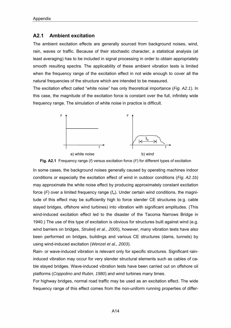
Appendix
A14
A2.1 Ambient excitation The ambient excitation effects are generally sourced from background noises, wind,
rain, waves or traffic. Because of their stochastic character, a statistical analysis (at
least averaging) has to be included in signal processing in order to obtain appropriately
smooth resulting spectra. The applicability of these ambient vibration tests is limited
when the frequency range of the excitation effect in not wide enough to cover all the
natural frequencies of the structure which are intended to be measured.
The excitation effect called “white noise” has only theoretical importance (Fig. A2.1). In
this case, the magnitude of the excitation force is constant over the full, infinitely wide
frequency range. The simulation of white noise in practice is difficult.
a) white noise b) wind
Fig. A2.1 Frequency range (f) versus excitation force (F) for different types of excitation
In some cases, the background noises generally caused by operating machines indoor
conditions or especially the excitation effect of wind in outdoor conditions (Fig. A2.1b)
may approximate the white noise effect by producing approximately constant excitation
force (F) over a limited frequency range (fw). Under certain wind conditions, the magni-
tude of this effect may be sufficiently high to force slender CE structures (e.g. cable
stayed bridges, offshore wind turbines) into vibration with significant amplitudes. (This
wind-induced excitation effect led to the disaster of the Tacoma Narrows Bridge in
1940.) The use of this type of excitation is obvious for structures built against wind (e.g.
wind barriers on bridges, Strukelj et al., 2005), however, many vibration tests have also
been performed on bridges, buildings and various CE structures (dams, tunnels) by
using wind-induced excitation (Wenzel et al., 2003).
Rain- or wave-induced vibration is relevant only for specific structures. Significant rain-
induced vibration may occur for very slender structural elements such as cables of ca-
ble stayed bridges. Wave-induced vibration tests have been carried out on offshore oil
platforms (Coppolino and Rubin, 1980) and wind turbines many times.
For highway bridges, normal road traffic may be used as an excitation effect. The wide
frequency range of this effect comes from the non-uniform running properties of differ-
f
F
f
F
fw

Appendix
A15
ent vehicles crossing the bridge. By the use of a statistical analysis during signal proc-
essing, the relative weight of the natural frequencies can significantly be amplified in
the averaged spectrums (Mazurek and DeWolf, 1990, Raghavendrachar and Aktan,
1992, Kálló, 1997, Kovács et al.,1998b). During the in-situ measurements, no restric-
tion or interruption of traffic is generally needed, which makes these tests cost-
effective. Therefore, these tests are often considered as parts of long-term monitoring
programs. A considerable number of papers deal with this topic in literature.
A2.2 Excitation by mechanical forces Excitation characteristics similar to that for wind can be achieved by using impact ham-
mers with changeable heads (e.g. PCB hammer). The excitation effect is induced by an
impact with this hammer. Depending on the applied head, the frequency range of the
excitation force (an example is shown in Fig. A2.2a) can coincide with the frequency
domain which includes all natural frequencies of the structure and are to be measured.
Therefore, due to the previously known and adjustable characteristics of the input
excitation data, these hammers are the most sufficiently and most frequently applied
excitation devices for controlled vibration tests in both field and laboratory conditions
(Raghavendrachar and Aktan, 1992, Mazurek and DeWolf, 1990).
In comparison to impact hammers, less than perfect excitation effects arise from simple
mechanical impulses. Theoretically, the magnitude of the amplitude (A) of the so called
“Dirac-δ” effect is infinite (A=∞); furthermore the duration of the amplitude-changes for
both the Dirac-δ and the ideal diminishing impulse equals zero (∆t=0) as shown in
Fig. A2.2b and Fig. A2.2c. The shape of the frequency spectrum corresponds to the
sin(x)/x function for the Dirac-δ effect and to the 1/x function for the ideal diminishing
impulse, therefore, the magnitude of the excitation force over the frequency scale is
proportional to the sin(x)/x function for the Dirac-δ effect and to the 1/x function for the
ideal diminishing impulse. Consequently, the intensity of the excitation force is much
higher in the lower frequency domains than in the higher domains. For real structures
and especially for bridges, these effects are simulated and approximated by simple
mechanical impacts with A≠∞ and ∆t≠0 represented by objects falling on or off the
structure to be excited, respectively (Illéssy, 1982).

Appendix
A16
a) PCB impact hummer (Raghavendrachar and Aktan, 1992)
b) Dirac-δ effect c) Ideal (diminishing) impulse effect
Fig. A2.2 Excitation characteristics for simple mechanical impulses
Sometimes exciters inducing periodic excitation force (e.g. machines with rotating ec-
centric mass) are used for both laboratory and field tests. In these cases the revolution
of the exciter can be changed and, consequently, can coincide with one of the natural
frequencies of the structure in order to cause resonance effects in the structural re-
sponse (Illéssy, 1982, Kovács and Farkas, 2000).
A3 LITERATURE REVIEW OF VIBRATION-BASED DAMAGE IDENTIFICATION METHODS A3.1 Damage identification based on changes in the basic modal parameters A3.1.1 Methods based on changes in the natural frequencies A3.1.1.1 Model-based methods
The forward problem
In the 1970s and the early 1980s many authors analysed offshore structures (oil plat-
forms and light stations) by numerical analysis. They modelled local damage by partly
xxa sin~
f, x
F A
t
A=∞
∆t=0x
b 1~
f, x
F A
t ∆t=0
Appendix
A17
or fully cutting structural elements. Depending on the modelled damage location, 1-2%
shifts in the natural frequencies were found to be indicative of damage (Coppolino and
Rubin, 1980). Cracks had little influence on global stiffness (Begg et al., 1976). Many
in-situ tests resulted in the conclusion that it was important to analyse natural fre-
quency shifts parallel to the associated mode shapes when trying to locate damage
(Kenley and Dodds, 1980).
Cawley and Adams (1979) detected single damage from frequency shifts on aluminium
and carbon-fibre-reinforced-plastic plates. They defined an error term that related to the
ratio between frequency shifts belonging to a pair of modes measured on the real
structure and calculated from a numerical model. The potential single damage was
modelled by local stiffness reductions; no possible multiple damage was considered.
The damage location was indicated when the considered frequency pairs minimized
the error form. Many mode pairs were taken into account. This sensitivity-based dam-
age localization procedure needed considerable computing time and capacity to pro-
duce ratios of frequency shifts for all possible damage locations. The accuracy of the
method depended on the quality of the numerical model. Similar work has been per-
formed by Penny, et al. (1993).
Ismail et al. (1990) pointed out by experiments that a crack in a concrete beam, which
periodically opens and closes, causes a smaller drop in the natural frequencies than a
continuously open crack. It concludes that the ratio between permanent and variable
loads also influences the magnitude of the crack-induced frequency shifts.
Brincker et al. (1995a) used statistical analysis to detect damage in concrete beams
with different steel ratios by ordering so-called “significance” indicators to every modal
frequency, as follows:
( )( ) ( )2id
f2i
uf
di
ui
if
σ+σ
−=
ffS (A3.1)
where (σf)i is the experimentally-determined standard deviation (SD) of the i-th natural
frequency. The u and d indices refer to the undamaged and the damaged states, re-
spectively. This indicator significantly increases for natural frequencies measured with
low SD that indicates the presence of a possible damage compared to the undamaged
state. A similar significance indicator was defined for the measured damping ratio. The
author also defined a “unified significance indicator” by summing the above frequency
and damping significance indicators over several measured modes. It was pointed out
that the significance indicators were sensitive to damage but were not capable of locat-
ing them. This technique was insensitive to the type of excitation (input signals).

Appendix
A18
Choy et al. (1995) developed an iterative procedure to detect and locate damage in
simply supported beams and for beams on an elastic foundation. Damage was mod-
elled by reducing the Young’s modulus of one element of the beam. They adjusted the
Young’s modulus of the considered element until the calculated natural frequency
matched the corresponding measured one. This procedure was repeated for each ele-
ment and for many natural frequencies. The location of the damage was obtained from
the intersection of the Young’s modulus reduction versus element location curves plot-
ted for each natural frequency (Fig. A3.1). This procedure has been extended for local-
izing multiple damage.
Fig. A3.1 Results of the damage locating iterative procedure developed by Choy et al. (1995)
However, without any information on the mode shapes associated with the measured
natural frequencies, this procedure is not able to distinguish between damage situated
in symmetric locations in symmetric structures as also shown in Fig. A3.1.
The inverse problem
Armon et al. (1994) applied a method to detect and localize cracks in beams using a
rank-ordering of modes according to the changes in the associated natural frequencies.
The method is based on the recognition that a forming crack often modifies the se-
quence of the fractional natural frequency shifts of a structure. A computer-simulated
result using the first four modes is shown in Fig. A3.2 for a cantilever beam.
Fig. A3.2 Fractional changes in natural frequencies versus crack location (Armon et al., 1994)

Appendix
A19
The authors declared that although rank-ordering was not sensitive to the crack size
(consequently it could not be used for damage quantification) it was also insensitive to
small uncertainties in boundary conditions and temperature changes as well as re-
quired moderate measurement accuracy. The method was experimentally studied on
cantilever Perspex and aluminium beams.
Stubbs and Osegueda (1990a, 1990b) used sensitivity analyses for beams to point out
how local damage, which was defined as reductions in the stiffness of one of the ele-
ments forming the structure, influences the natural frequencies. The damage localizing
procedure is built on the definition and the use of sensitivity matrices, which describe
the sensitivity of the frequency changes to changes in the element stiffness (and
mass). This method has been improved by including the effects of changes in damping.
The matrices were calculated by FEM, which demanded a considerable amount of
computation and the use of an accurate, previously-built numerical model.
Based on the work by Cawley and Adams (1979), Stubbs and Osegueda (1990a,
1990b) developed another damage detection method by including the sensitivity of
natural frequency change to changes in stiffness of local elements into the error term.
This improved method proved to be more accurate compared to their previous one
when the number of elements were much higher than the number of measured natural
frequencies.
Another damage localizing method has been developed by Hearn and Testa (1991)
and applied to a four-member welded steel frame subjected to cyclic loading and wire
ropes under constant tension. In both cases, concentrated, significant damage cases
were produced (fatigue crack and saw cut) in the verification tests. This method, again
similarly to the work by Cawley and Adams (1979), focused on the ratios of the natural
frequency shifts. They started from the eigenvalue problem of free vibration
(K-ω2M)φ = 0 (A3.2)
where K and M are the global stiffness and mass matrices, respectively; ω2 is the di-
agonal matrix containing the natural frequency squares and φ is the normalized mode
shape vector. Assuming that damage does not change the mass properties of the
structure and neglecting the second-order terms, the perturbation of Eq. (A3.2) results
in a relationship between the change in the i-th natural frequency and the damage-
induced change in the global stiffness as follows:
i
Ti
iiTi2
iφφφφ
MK∆
=ω∆ (A3.3)
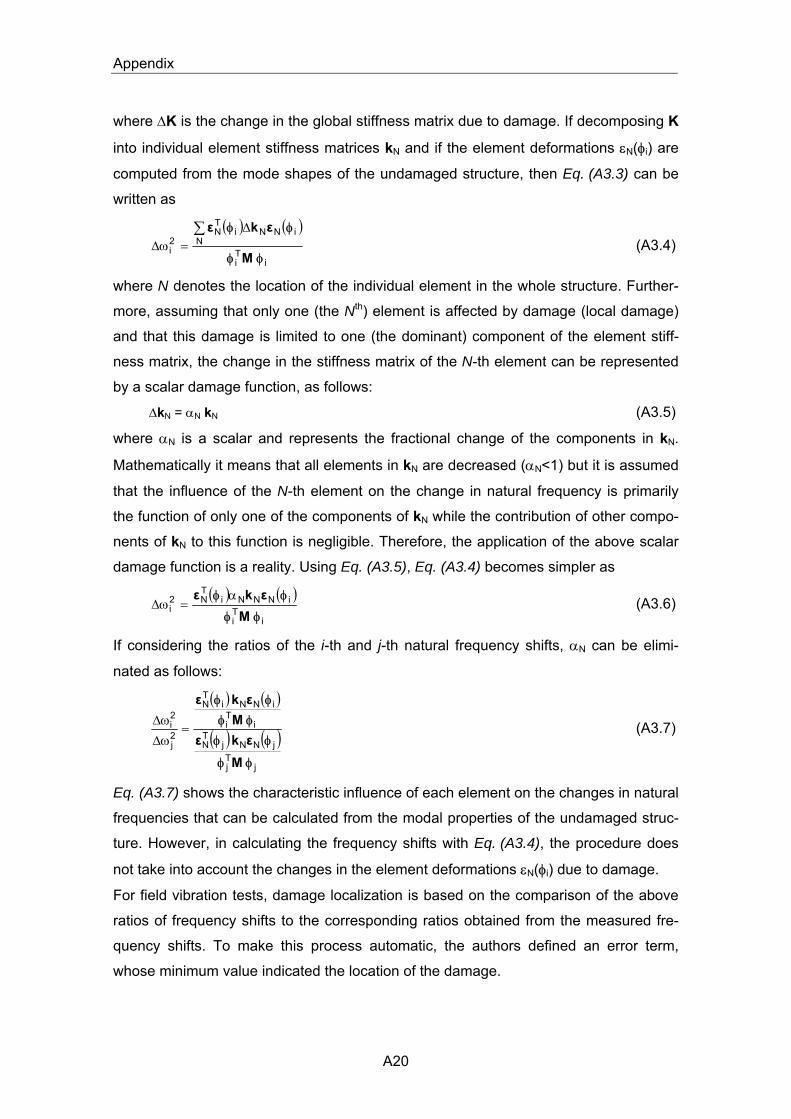
Appendix
A20
where ∆K is the change in the global stiffness matrix due to damage. If decomposing K
into individual element stiffness matrices kN and if the element deformations εN(φi) are
computed from the mode shapes of the undamaged structure, then Eq. (A3.3) can be
written as
( ) ( )
iTi
NiNNi
TN
2i
φφ
φφ
M
εkε∑ ∆=ω∆ (A3.4)
where N denotes the location of the individual element in the whole structure. Further-
more, assuming that only one (the Nth) element is affected by damage (local damage)
and that this damage is limited to one (the dominant) component of the element stiff-
ness matrix, the change in the stiffness matrix of the N-th element can be represented
by a scalar damage function, as follows:
∆kN = αN kN (A3.5)
where αN is a scalar and represents the fractional change of the components in kN.
Mathematically it means that all elements in kN are decreased (αN<1) but it is assumed
that the influence of the N-th element on the change in natural frequency is primarily
the function of only one of the components of kN while the contribution of other compo-
nents of kN to this function is negligible. Therefore, the application of the above scalar
damage function is a reality. Using Eq. (A3.5), Eq. (A3.4) becomes simpler as
( ) ( )i
Ti
iNNNiTN2
iφφ
φφ
Mεkε α
=ω∆ (A3.6)
If considering the ratios of the i-th and j-th natural frequency shifts, αN can be elimi-
nated as follows:
( ) ( )
( ) ( )j
Tj
jNNjTN
iTi
iNNiTN
2j
2i
φφ
φφφφ
φφ
Mεkε
Mεkε
=ω∆ω∆ (A3.7)
Eq. (A3.7) shows the characteristic influence of each element on the changes in natural
frequencies that can be calculated from the modal properties of the undamaged struc-
ture. However, in calculating the frequency shifts with Eq. (A3.4), the procedure does
not take into account the changes in the element deformations εN(φi) due to damage.
For field vibration tests, damage localization is based on the comparison of the above
ratios of frequency shifts to the corresponding ratios obtained from the measured fre-
quency shifts. To make this process automatic, the authors defined an error term,
whose minimum value indicated the location of the damage.

Appendix
A21
Richardson and Mannan (1992) tracked damage by calculating changes in the global
stiffness matrix. They determined a sensitivity equation for each mode based on the
orthogonality properties of the damaged and the undamaged structure. Assuming
again that mode shapes did not change due to damage, the difference between natural
frequency squares of the damaged (ωi,d2) and the undamaged (ωi,u
2) structure for the i-
th mode shape resulted in
φiT∆Kφi = ωi,d
2 - ωi,u2 (A3.8)
where notations are the same as for Eq. (A3.3). To calculate ∆K in Eq. (A3.8), the
mode shape and the natural frequency of the undamaged structure and the natural
frequency of the damaged structure are required. However, these equations often be-
come undetermined.
Brincker et al. (1995b) applied a so-called “auto-regressive moving average” (ARMA)
procedure to the measured acceleration-time histories of reinforced concrete offshore
platforms in order to estimate modal properties (frequencies and damping). The [n,m]
order ARMA model expresses the present structural response as a linear combination
of n past responses as well as the present and m past inputs as follows:
( ) ( ) ( ) ( ) ( ) ( )teiteidityictym
i
n
i+−−−= ∑∑
== 11 (A3.9)
where y(t) is the acceleration-time response at the present time t, y(t-i) are the re-
sponses at previous times, c(i) and d(i) are the auto-regressive (AR) and the moving
average (MA) parameters, respectively, e(t) and e(t-i) are the present and the past in-
puts assumed to be white noise. The AR and MA parameters are iteratively obtained
by minimizing an error term based on the measured and the predicted (by Eq. (A3.9))
responses. The roots of the polynomial can be related to the modal properties (fre-
quencies and damping).
Koh et al. (1995) presented a recursive method for damage localization in multi-storey
steel frame buildings using frequency measurements. The degrees of freedom of the
structure were reduced based on static considerations. Damage was modelled by local
stiffness reduction in particular columns.
Narkis (1994) presented analytical, closed formulas for determining the crack location
(e) in beams based on the measured shifts of any two natural frequencies (∆fi and ∆fj).
The parameter of these formulae is
ii
jjji ff
ffR
∆
∆= (A3.10)

Appendix
A22
where both the i-th and the j-th indices relate to either axial or flexural modes depend-
ing on which type of vibration is considered. For simply supported beams under flexure,
this formula is as follows:
⎟⎟⎠
⎞⎜⎜⎝
⎛−
π=
21arccos1 jiR
e (A3.11)
For the same beam under axial vibration (no restraint of the axial force at one end and
axially fixed other end):
⎟⎟
⎠
⎞
⎜⎜
⎝
⎛ −±
π=
21
arcsin2 jiRe (A3.12)
Similar equations can be defined for a combination of any two modes.
Morassi (2001) improved Narkis’ (1994) analytical results by using the knowledge that
for beams, the change in a natural frequency due to a single crack may be represented
as the product of two terms, of which the first is proportional to the severity (K) and the
second depends solely on the location (S) of the damage. Thus, this method was in-
tended for both damage localization and quantification of its severity. The modelled
crack was simulated by a linear spring with stiffness K connecting to the two segments
of the beam. He found that for beams with free ends under axial vibration, the ratio
between the changes in the 2m-th and the m-th natural frequencies explicitly deter-
mined the position variable (S) (for m=1, this formula matched with the corresponding
result achieved by Narkis (1994)) and the changes in the 2m-th and the m-th natural
frequencies allowed to explicitly determine the spring stiffness K. The theoretical re-
sults were confirmed by the results coming from axial vibration tests of suspended steel
beams with free-free ends. The beams were damaged by different notches. The author
noted that some of the results were also valid for beams under flexure.
Messina et al. (1998) localized damage in structures by defining Damage Location As-
surance Criterion (DLAC) for single damage cases and Multiple Damage Location As-
surance Criterion (MDLAC) for multiple damage cases, as follows:
DLAC(j) = ( )
( )( )jTj
T
2j
T
ffffff
δδ∆∆
δ∆ (A3.13a)
MDLAC(δD) = ( )( )( ))()(
)(TT
2T
DfDfffDff
δδδδ∆∆δδ∆ (A3.13b)
where ∆f is the measured natural frequency change vector of the structure with a single
damage of unknown size and δfj is the calculated natural frequency change vector for a
damage of known size at location j. For the multiple damage case, δD is the change of

Appendix
A23
the global stiffness matrix containing the individual stiffness reductions of one or more
elements in any locations and δf(δD) contains the calculated natural frequency
changes due to δD. This part of their work, which integrated the measured and the
(analytically or numerically) calculated changes in the natural frequencies into one indi-
cator value, was only an improvement of the original results achieved by Cawley and
Adams (1979). The DLAC and MDLAC values are very similar to the Modal Assurance
Criterion (MAC) value used for comparing mode shapes (see Sect. A3.1.2.1). However,
the authors developed this method and defined coefficients for estimating the size of
the damage both for single and multiple damage cases. The reliability of the MDLAC
was confirmed by analytical examples as well as by experiments carried out on an
aluminium frame model.
A3.1.1.2 Non-model-based methods
Kato and Shimada (1986) conducted ambient vibration tests on a statically preloaded,
full scale prestressed concrete bridge. The structure was subjected to gradually in-
creasing, controlled static loads in four loading steps up to failure. They found small
change in the vibration characteristics while the prestressing tendons were in the elas-
tic stage even when cracking occurred. This was explained by the cracks closing to-
gether by the effective prestressing after the load was removed. After the tendons ex-
ceeded the elastic limit a sudden decrease in the natural frequencies was observed,
which continued as the failure progressed. It was concluded that this observation of-
fered the possibility of discovering tendon weaknesses in prestressed concrete bridges.
Salawu (1997b) defined a Global Integrity Index (GI) for detecting changes in the struc-
tural integrity (mass or stiffness) of CE structures as follows:
∑⎥⎥⎦
⎤
⎢⎢⎣
⎡⎟⎟⎠
⎞⎜⎜⎝
⎛ωω
=r
aGIr0
Drr (A3.14)
where ωDr and ω0r are the natural frequencies associated with the mode r and referred
to the damaged and the undamaged structure, respectively. Values of GI other than 1,0
indicated a change in the structural integrity. The ar is a weighting factor of the r-th
mode that depended on the dominance of the considered mode in the dynamic re-
sponse of the structure. It was suggested that at least (the most dominant) three
modes should have been considered with the corresponding ar values equal to 0.7, 0.2
and 0.1 in the sequence of their dominance. The most dominant modes were selected
by using the Modal Sensitivity Value (MSV) defined as:

Appendix
A24
{ } { }( )
( ) ( )
( )2r0
2ir0
2r0
2ir0
2Dr
2Dir
rDr0 ,
ω
φ
ω
φ−
ω
φ
=φφ∑
∑∑
i
ii
MSV (A3.15)
where φ0ir and φDir are the elements of the r-th mode shape vector at measurement
point i belonging to the undamaged and the damaged state, respectively. The highest
MSV indicates the most dominant mode. For selecting dominant modes, the use of the
MSV is alternative to the use of the Modal Assurance Criterion (MAC, see
Sect. A3.1.2.1). Because only natural frequencies are included in Eq. (A3.14), theoreti-
cally, one measurement point is sufficient. The author completed this method by defin-
ing a Local Integrity Index (LIi) for each measurement point to locate and quantify local
damage (see Sect. A3.1.2.1).
A3.1.2 Methods based on changes in the mode shapes and in their derivatives
A3.1.2.1 Methods using displacement mode shapes
Model-based methods
Yuen (1985) defined mode shape and mode-shape-slope parameters by combining the
mode shape amplitudes and the associated natural frequencies of the damaged and
the undamaged structure, and examined their changes due to numerically simulated
stiffness reductions (as models of localized damage) in each structural element for a
cantilever beam. Then these predicted changes were compared to the corresponding
measured changes to determine the damage location in the investigated structure. This
method can be considered as a classical solution for the forward problem
(Sect. A3.1.1.1) using mode shape data.
An example for the solution of the inverse problem was given by Rizos et al. (1990)
who presented an analytical method, which was used to predict the position and the
depth of a single, open crack along a cantilever steel beam. The authors established a
non-linear system of equations for the harmonically vibrating beam divided into two
parts by a bending spring, which represented an open crack, the spring constant of
which was calculated on the basis of the crack-strain-energy function. Having the ex-
perimentally measured amplitude-time function of the beam forced into harmonic vibra-
tion at one of the natural frequencies, the analytical solution resulted in the crack pa-
rameters (location and depth) as unknowns. The mode shapes were recorded at only
two locations. The differences between the computed and the precisely checked crack
parameters remained below 8%. The authors noted that the analytical model can be

Appendix
A25
substituted by an appropriate finite element model. It was also concluded that the
method lacked accuracy for small cracks (where the crack depth was smaller than
1/10-th of the cross-section depth) and for more complex structures (with multiple
cracks). Therefore, for real structures this method was intended only to locate and
quantify single cracks.
Non-model-based methods
MAC indicates correlation between two modes including mode shape amplitudes
gained from each measurement point:
{ } { }( )( )( )
( ) ( )∑∑
∑
==
=
φφ
φφ=φφ nn
n
MAC
1i
2Bir
1i
2Aiq
2
1iBirAiq
rBqA , (A3.15)
where φAiq (φBir) are the element of the A-th (B-th) set of mode shape vectors for the q-
th (r-th) mode belonging to the i-th measurement point and n is the total number of
measurement points. If MAC is used as a damage indicator, the considered mode
shapes in Eq. (A3.15) belong to the same mode measured before and after the as-
sumed damage event. The MAC value can vary between 1,0 and 0,0, where the 1,0
value indicates full correlation and the 0,0 value indicates no correlation between the
considered mode shapes. Because mode shape amplitudes gained from all measure-
ment points are included into Eq. (A3.15), MAC can be considered as a global damage
indicator. Therefore, often MAC proves to be insensitive to local damage.
COMAC contains local information on the vicinity of the considered measurement loca-
tion because it includes two sets of amplitudes of all recorded mode shapes at the i-th
measurement point as follows:
( )( )( )
( ) ( )∑∑
∑
==
=
φφ
⎟⎟⎠
⎞⎜⎜⎝
⎛φφ
= mm
m
COMAC
1r
2Bir
1r
2Air
2
1rBirAir
i,B,A (A3.16)
where φAir (φBir) is the element of the A-th (B-th) set of mode shape vectors for the r-th
mode belonging to the i-th measurement point and m is the number of the recorded
mode shapes. If COMAC is used as a damage indicator, the considered sets of mode
shape amplitudes in Eq. (A3.16) are measured before and after the assumed damage
event. The COMAC value can also vary between 1,0 and 0,0, where the 1,0 value indi-
cates full correlation and the 0,0 value indicates no correlation between the considered
sets of mode shape amplitudes.

Appendix
A26
Allemang (2003) gave a thorough overview on the theoretical background and the ex-
perience of application of MAC together with many other related assurance criteria
used in the field of experimental modal analysis.
Salawu and Williams (1995) used MAC and COMAC to compare the mode shapes of a
multispan reinforced concrete highway bridge before and after a local structural repair.
Artificial excitation of the bridge was achieved by a special excitation system giving a
periodic random signal. The authors concluded that for an appropriate measurement
point arrangement MAC can be used to indicate the existence of any change in the
mode shapes (Level 1) as well as to select mode shapes which are mostly influenced
by this change. However, due to their local character, COMAC values give better in-
formation on the location of this change (Level 2) than MAC values, therefore COMAC
values can effectively be used for damage detection and localization as well. The au-
thors also suggested that the quantification (Level 3) of the change detected and local-
ized by the use of MAC and COMAC should have been examined by other routine,
local non-destructive techniques.
A similar damage localization approach for CE structures was introduced by Salawu
(1997b) as an improvement of the Global Integrity Index (GI) method (see
Sect. A3.1.1.2). The author noted that due to its global nature, GI (similarly to MAC)
was not sensitive enough to local defects, therefore the Local Integrity Index (LI) was
defined at the i-th measurement point and includedmode shape data into the LI index
as follows:
∑⎥⎥
⎦
⎤
⎢⎢
⎣
⎡
⎟⎟
⎠
⎞
⎜⎜
⎝
⎛
φ
φ⎟⎟⎠
⎞⎜⎜⎝
⎛ωω
=r 2
2
r0
Drri
ir0
DiraLI (A3.17)
where φDir (φ0ir) is the element of the r-th mode shape vector belonging to the i-th
measurement point for the damaged and the undamaged structure, respectively. Exis-
tence of any damage (loss of integrity) at point i is likely if ⏐LIi – 1⏐ > 0 and unlikely if
⏐LIi – 1⏐ = 0. For practical applications, values of ⏐LIi – 1⏐ for points most likely to be
damage locations are much larger than those for points in undamaged areas. To define
mode shapes and to locate the defective areas with the LIi index, a sufficient number of
measurement points is required. For practical applications, authors suggested to calcu-
late GI first. If damage (loss of integrity) is detected by the GI then LIi should be calcu-
lated at a few widely spaced points. The GI and LIi indices can be calculated very sim-
ply without extensive computation effort. The GI and LIi indices were verified by a nu-
merical example and an experimental test conducted on a steel beam deteriorated by
saw cuts.

Appendix
A27
Dong et al. (1994) studied the applicability of mode shapes based on direct strain
measurements (strain mode shapes) according to Eq. (A3.18), instead of curvature
mode shapes (see Sect. A3.1.2.2) calculated from displacement mode shapes, by de-
fining a new parameter formulated as:
{∆φ*}i = {φd}i 2
di
ui⎟⎟⎠
⎞⎜⎜⎝
⎛
ωω
- {φu}i (A3.18)
where {φu}I and {φd}I are the amplitudes of the i-th strain mode shape for the undam-
aged and the damaged beam, respectively, while ωiu and ωi
d are the associated natural
frequencies. The authors proved that, thanks to the combination of the mode shape
changes with the associated natural frequency shifts, this parameter was more sensi-
tive to damage than the equivalent indices computed only from displacement mode
shape data.
Topole and Stubbs (1995) introduced a damage prediction method based on matrix
structural analysis using limited modal information on the damaged structure. Instead
of previous knowledge of modal information of an undamaged structure, only estimates
of masses and stiffnesses based on geometrical data of the initial structure were re-
quired. They found, and numerically verified on a 10-storey model building, that struc-
tural damage, assumed to be a local reduction in stiffness, could be correctly detected,
located and quantified from available measured information of approximately NE
modes, where NE denotes the number of structural elements. They suggested that the
experimentally measured modal data could be more efficiently used for this case than
in methods using MAC according to Eq. (A3.15).
A3.1.2.2 Methods based on mode shape curvature
Pandey et. al. (1991) first computed the displacement mode shapes of a cantilever and
a simply supported beam numerically by finite element analysis and then compiled the
corresponding curvature mode shapes by calculating the curvature at each element
(ρq,i) by using the central difference approximation as follows:
ρq,i = φq,i’’ = 2q
i,1qi,qi,1q 2
h+− φ+φ−φ
(A3.19)
where φq-1,i, φq,i and φq+1,i are the corresponding amplitudes of the i-th displacement
mode shape in the vicinity of the q-th element and hq is the length of this q-th element.
Damage was numerically modelled by reducing the Young’s modulus (E) in the corre-
sponding element(s) of the beam and then identified and quantified by the comparison
between the curvature mode shapes for the undamaged and the damaged structure.

Appendix
A28
They found that curvature mode shapes are much more sensitive to local damage than
either displacement mode shapes (Fig. A3.3) or even the MAC and the COMAC val-
ues.
a) b)
Fig. A3.3 Absolute difference between a) curvature mode shapes b) displacement mode
shapes for the damaged and the undamaged simply supported beam (for 50% reduction in E at
point No.13) by Pandey et al. (1991)
A very similar work has been conducted by Ratcliffe (1997) for beams with discrete
mode shapes (recorded at discrete points). He showed that the Laplacian operator
itself formulated similarly to Eq. (A3.19) as
L i = (φi-1 + φi+1) - 2φi (A3.20)
and, when applied to a discrete displacement mode shape, was able to successfully
indicate the presence and even the location of damage (modelled by stiffness reduction
at one of the discrete points) for severe damage cases without the knowledge of the
mode shape of the undamaged structure. For less severe damage cases, difference
functions, defined as the difference between the Laplacian and a cubic polynomial fit-
ted to the Laplacian locally around each discrete point, provided the necessary infor-
mation on the damage location. The method was demonstrated on a finite element
beam model and was experimentally verified on a suspended steel beam. Because the
Laplacian represented the local curvature of the displacement mode shape and the
surface strain was proportional to the curvature according to Eq. (1.1), the author sug-
gested replacing the Laplacian by the experimentally measured strain mode shapes for
damage identification purposes on real structures.
Salawu and Williams (1994) demonstrated that when using experimental data the cur-
vature change did not typically give a good damage indication. They emphasized the
importance of selection of which mode shapes are to be used in the analysis.
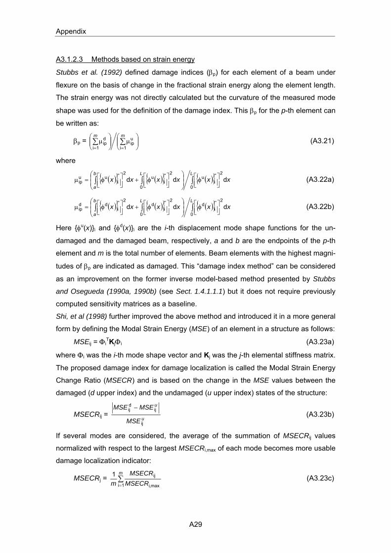
Appendix
A29
A3.1.2.3 Methods based on strain energy
Stubbs et al. (1992) defined damage indices (βp) for each element of a beam under
flexure on the basis of change in the fractional strain energy along the element length.
The strain energy was not directly calculated but the curvature of the measured mode
shape was used for the definition of the damage index. This βp for the p-th element can
be written as:
βp = ⎟⎟⎠
⎞⎜⎜⎝
⎛µ⎟⎟
⎠
⎞⎜⎜⎝
⎛µ ∑∑
==
mm
1i
uip
1i
dip (A3.21)
where
( ){ } ( ){ } ( ){ }∫∫∫ ⎥⎦⎤
⎢⎣⎡ φ⎟
⎟⎠
⎞⎜⎜⎝
⎛⎥⎦⎤
⎢⎣⎡ φ+⎥⎦
⎤⎢⎣⎡ φ=µ
LLb
axxxxxx
0
2''i
u
0
2''i
u2''
iuu
ip ddd (A3.22a)
( ){ } ( ){ } ( ){ }∫∫∫ ⎥⎦⎤
⎢⎣⎡ φ⎟
⎟⎠
⎞⎜⎜⎝
⎛⎥⎦⎤
⎢⎣⎡ φ+⎥⎦
⎤⎢⎣⎡ φ=µ
LLb
axxxxxx
0
2''i
d
0
2''i
d2''
idd
ip ddd (A3.22b)
Here {φu(x)}i and {φd(x)}i are the i-th displacement mode shape functions for the un-
damaged and the damaged beam, respectively, a and b are the endpoints of the p-th
element and m is the total number of elements. Beam elements with the highest magni-
tudes of βp are indicated as damaged. This “damage index method” can be considered
as an improvement on the former inverse model-based method presented by Stubbs
and Osegueda (1990a, 1990b) (see Sect. 1.4.1.1.1) but it does not require previously
computed sensitivity matrices as a baseline.
Shi, et al (1998) further improved the above method and introduced it in a more general
form by defining the Modal Strain Energy (MSE) of an element in a structure as follows:
MSEij = ΦiTKjΦi (A3.23a)
where Φi was the i-th mode shape vector and Kj was the j-th elemental stiffness matrix.
The proposed damage index for damage localization is called the Modal Strain Energy
Change Ratio (MSECR) and is based on the change in the MSE values between the
damaged (d upper index) and the undamaged (u upper index) states of the structure:
MSECRij = u
u
MSE
MSEMSE
ij
ijdij −
(A3.23b)
If several modes are considered, the average of the summation of MSECRij values
normalized with respect to the largest MSECRi,max of each mode becomes more usable
damage localization indicator:
MSECRj = ∑=
m
MSECRMSECR
m 1i max,i
ij1 (A3.23c)

Appendix
A30
where m denotes the considered number of modes. For damage quantification pur-
poses in practical applications Shi, et al (2000) extended their method by a MSE sensi-
tivity analysis. This approach required the elemental stiffness matrices, the analytical
(or numerically calculated) mode shapes and the incomplete measured mode shapes
as input data. First the incomplete measured mode shapes are expanded by the use of
the analytical mode shapes, then the damage coefficient αj, which measures the frac-
tional change in the j-th elemental stiffness matrix, is calculated by an iterative process.
The applicability of MSECR values for damage localization and that of the latter sensi-
tivity analysis for damage quantification were demonstrated on numerical examples
(cantilever and fixed beams) and on an experimental two-storey steel frame.
A3.1.3 Methods based on changes in damping parameters Tests carried out on an ordinary steel-concrete composite bridge by Farrar and
Jauregui (1998), on concrete beams with artificially made crack-modelling cuts by
Casas and Aparicio (1994) and on a continuous, reinforced concrete, voided slab
bridge before and after a structural repair by Salawu and Williams (1995) indicated no
clear relationship between local damage growth and damping changes. It seemed for
each case that damage influenced the damping ratios associated with different modes
in different ways. Salane and Baldwin (1990) found from the results of a fatigue test
conducted on a three-span, steel-concrete composite bridge that the damping ratio
initially increased then subsequently decreased with increasing fatigue damage for all
of the first three investigated modes. However, when dynamically testing a similar, one-
span composite laboratory bridge model and cutting the bottom flange of one of the two
girders in a section, the modal damping ratio decreased for the first three modes.
Zonta et al. (2008) suggested that damping changes in concrete structures were
closely associated with friction mechanisms (i) at the concrete interfaces during closing
and opening of cracks and (ii) in the bond area between the concrete in tension and the
tension reinforcement. Consequently, no significant damping changes should be ex-
pected for structures where no significant cracking occurs due to damage. This was
observed on a five-storey experimental building designed to resist against earthquake
according to the capacity-based design theory (appropriately distributed, dissipative
plastic hinges with no friction damping effects and definitely linear post-earthquake
behaviour outside the plastic hinges).
Curadelli et al. (2008) used the continuous wavelet transform to identify the instantane-
ous damping coefficient on one numerical (three-bay, six storey reinforced concrete
frame excited by a known earthquake time history) and two experimental (a shock-
Appendix
A31
excited, simply-supported reinforced concrete beam and a one-bay, six-storey alumin-
ium frame excited on a shaking table) structures before and after damage. They found
that damping increased parallel to damage for each case and can be a useful damage
index for structures showing growing non-linearity due to increasing damage.
A3.2 Damage identification methods based on dynamically meas-ured flexibility The flexibility-based methods can be classified on the basis of the procedure applied in
indicating changes in the flexibility matrix of the structure.
A3.2.1 Differentiation of methods The methods based on the simple comparison of changes in the flexibility matrix and
its derivatives deal mainly with the non-model-based estimation of the flexibility coeffi-
cients from only on-site measured data. Raghavendrachar and Aktan (1992) computed
11 scaled mode shapes and then directly transformed them into flexibility without as-
suming a mass matrix after a multi-reference impact test on a three-span RC slab
bridge. They also observed that torsional modes and local modes with frequencies
comparable to those of global modes influenced the flexibility significantly. Therefore,
flexibility proved to be a sensitive indicator of both global and local damage. The results
have been confirmed by a FE model. Similar work has been performed by Pandey and
Biswas (1994) and (1995) on the analytical and the experimental models of steel
beams with different support conditions.
Later this method was improved by demonstrating on mainly bridge superstructures
that virtually “loading” the flexibility matrix by different load patterns and calculating the
“deflected” shapes by selecting and summing the corresponding elements of the flexi-
bility matrix results in new, more powerful and engineer-like damage indices such as
“uniform load surface” (Zhang and Aktan, 1995)) and “bridge girder condition indicator”
(Catbas and Aktan, 2002)).
The unity check method uses the inverse relationship between the flexibility [G] and the
stiffness [K] matrices to define an error matrix [E] as follows
[E] = [Gd] [Ku] – [I] (A3.24)
where the information on the damage is collected in [Gd] and the [Ku] is fixed to the
undamaged (or a previous baseline) structure. The positions of the elements in [E] that
differ from the unity and the magnitude of these differences relate to the position and
the degree of damage in the structure. This method was introduced by Lin (1994).

Appendix
A32
The stiffness error matrix method is an improvement of the unity check method. Here
the effect of measured flexibility changes between the damaged and the undamaged
(or the previous baseline) structures are transformed into stiffness changes as follows
[E] = [Ku] ([Gd] – [Gu]) [Ku] (A3.25)
which is measured by the computed stiffness error matrix [E].
A3.3 Matrix update methods A3.3.1. Mathematical background The governing rule is the minimization of the “modal force error” ({E}i), which comes
from the structural equation of motion given as:
[Mu]{ x&& } + [Cu]{ x& } + [Ku]{ x } = {f(t)} (A3.26)
and its eigenvalue equation for free vibration given as:
(( uiλ )2[Mu] + ( u
iλ )[Cu] +[Ku]) {φu}i = {0}, (A3.27)
where uiλ and {φu}i are the i-th natural frequency and the associated mode shape while
[Mu], [Cu] and [Ku] are the mass, the damping and the stiffness matrix (property matri-
ces) of the undamaged structure, if the measured modal data of the damaged structure
( diλ and {φd}i) are substituted into Eq. (A3.27) as follows:
(( diλ )2[Mu] + ( d
iλ )[Cu] +[Ku]) {φd}i = {E}i (A3.28)
In fact, this modal force error represents the harmonic force excitation of the undam-
aged structure, which would have to be applied with frequency diλ to get {φd}i mode
shape response. The iteration ends, and consequently the update is finished, if such
[Md], [Cd] and [Kd] matrices are found, which fulfil Eq. (A3.27) written for the undam-
aged structure as follows:
(( diλ )2[Md] + ( d
iλ )[Cd] +[Kd]) {φd}i = {0} (A3.29)
The solution is based on the definition of the damaged model matrices as the undam-
aged model matrices minus a perturbation as follows:
[Md] = [Mu] – [∆M]
[Cd] = [Cu] – [∆C] (A3.30)
[Kd] = [Ku] – [∆K]
After substituting Eq. (A3.30) into Eq. (A3.29) and moving the perturbation terms to the
left hand side of the equation, then the right hand side will be the same as the left hand
side of Eq. (A3.28) and so the modal error force can be written as follows:
(( diλ )2[∆M] + ( d
iλ )[∆C] +[∆K]) {φd}i = {E}i (A3.31)
Appendix
A33
The developed methods generally apply constraints regarding the property matrices in
order to simplify the solution of Eq. (A3.31). The most frequently applied constraints are
the preservation of symmetry in the [∆M], [∆C] and [∆K] matrices, the use of the same
zero/non-zero pattern in the [Md], [Cd] and [Kd] matrices as in [Mu], [Cu] and [Ku] as well
as the preservation of matrix positivity for the [∆M], [∆C] and [∆K] matrices (e.g.
{x}T[∆M]{x} ≥ 0).
A3.3.2. Differentiation of methods The elaborated matrix update methods differ in the mathematical procedures that are
applied to solve Eq. (A3.31).
The optimal matrix update methods directly compute either the property matrices of the
damaged structure or the perturbation matrices given in Eq. (A3.30) and give them in a
closed form. The problem is generally formulated as a Lagrange multiplier or a penalty-
based optimization. These methods are thoroughly reviewed by Zimmermann and
Smith (1992).
The sensitivity-based update methods solve a first-order Taylor-series that minimizes a
defined error function of the perturbation matrices ([∆M], [∆C] and [∆K]). The essence
of this theory is the determination of a modified parameter vector (consisting of material
and/or geometrical parameters) such as
{p}(n+1) = {p}(n) + {δp}(n+1) (A3.32)
in which the parameter perturbation vector {δp}(n+1) is computed from the Newton-
Raphson iteration when minimizing an error form, which is typically selected as the
modal force error according to Eq. (A3.28). These sensitivity-based techniques are
summarized by Hemez and Farhat (1995).
The eigenstructure assignment methods are based on the determination of a fictitious
term interpreted as a matrix perturbation to the undamaged model, which minimizes
the modal force error. If this term (e.g. the perturbation of the [Ku] stiffness matrix) is
selected such that the modal force error between the FE models of the undamaged
structure and the measured, damaged structure is equal to zero, then “best achievable
mode shape vectors” ({ daφ }i) can be determined as functions of the measured mode
shape vectors ({φd}i). The location and the severity of damage is concluded from the
relationship between { daφ }i
and {φd}i. These methods are overviewed by Lim (1995).
Due to the strong mathematical basis and the refined numerical techniques used, it is
obvious that these methods require significant computation capacity. For this reason
the hybrid methods were introduced by combining a computationally efficient optimal

Appendix
A34
matrix update method to locate the vicinity of the damage in the structure with a sensi-
tivity-based method to fix the damaged point by updating only small number of parame-
ters. Doebling, et al (1997a) experimentally analysed which modes of the damaged
structure have to be used when updating the FE model if the computation capacity is
limited. They found that modes storing the highest strain energy over the entire (dam-
aged) structure are the most indicative of damage and that selection of modes based
on maximum strain energy always provides more accurate model update than using
modes with lowest modal frequency. These results came from the test of a steel truss.
A3.4 Non-linear damage identification methods Lin and Ewins (1990) localized non-linearity in structures by using model update tech-
niques by neglecting the effect of structural damping. By conducting modal tests at two
different response levels a and b, Eq. (A3.29), with the inclusion of Eq. (A3.30), can be
written as follows:
(( aiλ )2[Mu + ∆M] + [Kd + ∆K ]) {φa}i = {0} (A3.33a)
(( biλ )2[Mu + ∆M] + [Kd + ∆K + ∆Kn]) {φb}i = {0} (A3.33b)
where aiλ , {φa}I and b
iλ , {φb}i are the i-th natural frequency and the associated mode
shape at response levels a and b, respectively. The [∆M] and [∆K] matrix perturbations
represent the FE model update and [∆Kn] represents the non-linearity in stiffness (here
the non-linearity in mass is neglected). If considering {φb}i as the perturbation of {φa}i
and that the modelling errors (λi)2[∆M] and [∆K] are of the same orders as [∆Kn] then
after multiplying Eq. (A3.33a) and Eq. (A3.33b) by {φb}iT and {φa}i
T, respectively, the
following result is obtained:
[∆Kn] {φb}i {φa}iT = [A] (A3.34)
where [A] is a known matrix calculated from the property matrices of the undamaged
model ([M], [K]) and the modal data measured at two response levels on the damaged
structure ( aiλ , {φa}I and b
iλ , {φb}i). This means that the non-linear term [∆Kn] may be de-
termined from [A] and the measured modal data.