Embed Size (px)
Citation preview
Creating Generative Models from Range Images
Ravi RamamoorthiStanford University∗
James ArvoCalifornia Institute of Technology
Abstract
We describe a new approach for creating concise high-level gener-ative models from range images or other approximate representa-tions of real objects. Using data from a variety of acquisition tech-niques and a user-defined class of models, our method produces acompact object representation that is intuitive and easy to edit. Thealgorithm has two inter-related phases:recognition, which choosesan appropriate model within a user-specified hierarchy, andparam-eter estimation, which adjusts the model to best fit the data. Sincethe approach is model-based, it is relatively insensitive to noise andmissing data. We describe practical heuristics for automaticallymaking tradeoffs between simplicity and accuracy to select the bestmodel in a given hierarchy. We also describe a general and efficienttechnique for optimizing a model by refining its constituent curves.We demonstrate our approach for model recovery using both realand synthetic data and several generative model hierarchies.
CR Categories: I.3.5 [Computer Graphics]: Ob-ject Modeling—Curve, surface, solid, and object representations,Object hierarchies, Splines; I.4.8 [Image Processing and ComputerVision]: Scene Analysis—Object Recognition, Surface Fitting
Keywords: Generative Models, Range Images, Curves and Sur-faces, Procedural Modeling
1 Introduction
It has recently become feasible to acquire reasonably accuratepoint-clouds orrange datafrom 3D objects [5, 26]. For graph-ics applications, these point-clouds are usually transformed intopolygonal meshes [5, 12], or spline patches [14]. However, theseapproaches often provide an unintuitive representation that is diffi-cult to manipulate once generated. In addition, a large amount ofdata is required since the meshes usually contain thousands of tri-angles. For modeling many man-made objects,generative modelsproposed by Snyder [21, 22] provide an attractive alternative. Agenerative model is a generalization of a swept surface in which
∗Address: Gates Wing 3B-372, Stanford University, Stanford, Ca 94305.
Figure 1: Generative models recovered from actual range data. Objectswere scanned individually, modeled using our algorithm, then composed inthis scene with artificial color and shading. A smooth compact represen-tation was generated for each object from a few simple model hierarchies,despite noisy and incomplete data. See figure 7 for a comparison of rangedata and recovered models.
the generating curve can be continuously transformed by one ormore arbitrary curves. For instance, a banana-like shape is speci-fied parametrically by translating a cross-section while scaling androtating it. The cross-section, scaling function, and rotation areall described by curves. The modeled object is analytically repre-sented by a tree of operators that provides a logical description ofits structure. Designers can easily construct, examine, and modifysuch a model.
We describe a method for inverting this process to recover gen-erative models from range data or other approximate representa-tions of object geometry. This method requires the user to specifya universe of possible objects by providing a hierarchy of shape op-erators defining a class of generative models. Given a user-definedhierarchy, such as the ones shown at the bottom of figure 2 andin figure 8, the system automatically selects a parametric modelwithin this hierarchy, and adjusts its parameters to best match dataacquired from an actual object. Several models recovered in thisway are shown in figure 1.
Our approach for model construction has a number of benefits:
Simplicity: Range data may be obtained by several methods,including theshadowapproach of Bouguet and Perona [2], that re-quires only a lamp, pencil and checkerboard apart from the camera.
Robustness: By exploiting redundancies in the data, accuratemodels can often be recovered from incomplete and noisy data.Our model-based approach is thus much less sensitive to noise thanmesh creation. Many of our examples use only one noisy and in-complete range image, while creation of a polygon mesh generallyrequires many accurate and properly aligned range images.
construction ofgenerative model
shadow method
structured light
3D point cloud
model hierarchy
best approximation
modified object
modelrecognition
parameterestimation
mechanical probe
curve editor
generativemodel
3D point cloud acquisition
root
shape benddepth
shape+bend +bend
depth+depthshape
Spoonlaser scanner
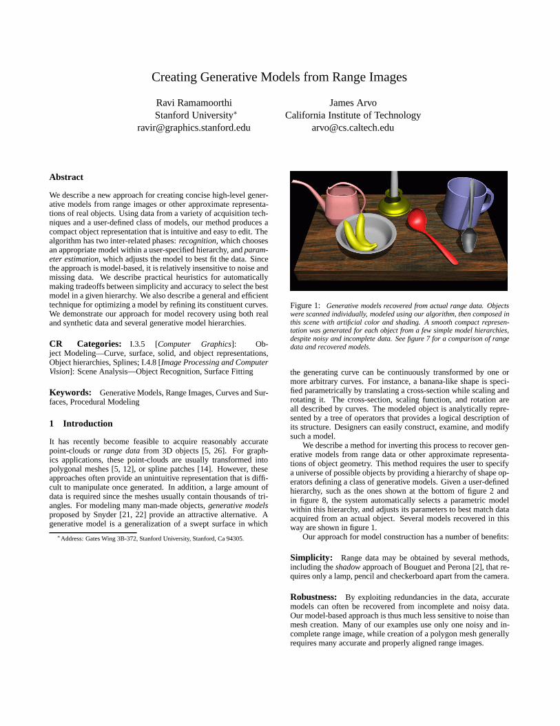
Figure 2:Overview of generative model creation. The algorithm takes range data in the form of a point-cloud and a generative model hierarchy as input. Anappropriate model is then chosen, and parameters are optimized to output an accurate and concise generative model that can subsequently be edited.
Compactness: Generative models provide a concise represen-tation; we need only store an algebraic model description, and con-trol points of the model’s parametric curves. This representationcan be orders of magnitude smaller than a triangle mesh.
Intuitiveness: Since the model is expressed in terms of para-metric curves corresponding to logical features of the object, it iseasy to understand, manipulate, and edit.
Related Work
Many methods have been explored, especially in computer vision,for recovering object shape for specific primitives such as gener-alized cylinders [1, 15], superquadrics [16, 23] and blended de-formable models [7]. Terzopoulos and Metaxas [24] have proposeda computational physics framework for shape recovery in whichglobally deformed superquadrics model coarse shape and local de-formations add fine detail. Superquadrics have also been used formodel-based segmentation [9, 11], and for recognition of “geons”using relationships between superquadric parameters [19, 27]. De-Carlo and Metaxas [8] introduced shape evolution with blending torecover and combine superquadrics and supertoroids into a unifiedmodel. Debevec et a. [6] considered architectural scenes and devel-oped a system for recovering polyhedral models from photographs.
Our approach is somewhat more general than these previous al-gorithms in that it is based on a general user-specified generativehierarchy rather than a particular parametric model. This allowsautomatic construction of more complex and varied shapes, with-out segmentation, than is possible with current computer vision al-gorithms. Further, many standard primitives used in computer vi-sion can be recovered using our method since generative modelsare a superset of traditional shape representations such as globallydeformed superquadrics, straight homogeneous generalized cylin-ders, and blended deformable models, all of which have been re-covered using our system. Our method is also automatic, with nouser intervention required. However, model-specific algorithms,especially those that allow user-intervention, may out-perform ouralgorithm on the shapes to which they apply by exploiting model-specific information. For instance, by considering only polyhedralmodels, and having the user manually specify the edges of interest,Debevec et al. [6] are able to work with only photographs, whilewe require range data.
This paper deals primarily with shapes represented by a sin-gle generative model. At present, we do not add local detail [24],nor address automatic model-based segmentation [8, 9, 11] or im-age interpretation [3]. However, our results suggest that generativemodels may be useful for these tasks in lieu of superquadrics orgeneralized cones.
In contrast to some object recognition methods [19, 27],whichestimate specific model parameters to classify an object as a mem-ber of some class, our method first determines which degrees offreedom in the model hierarchy are most suitable for the acquireddata, and then refines the associated parameters.
Recent work on simplifying polygonal meshes shares one ofour objectives—providing a more compact representation. For ex-ample, Hoppe et al. describe techniques to optimize meshes [13],while Eck and Hoppe [10] and Krishnamurthy and Levoy [14] fitspline surfaces to dense meshes. However, mesh-based methods donot yield compacthigh-levelmodels.
The rest of this paper is organized as follows: Section 2 givesan overview of our algorithm and describes our framework for re-covering the appropriate model within a user-specified hierarchy.In section 3, we discuss our methods for optimization. Section 4briefly outlines the various models used in our tests. In section 5,we discuss our results and section 6 presents our conclusions anddirections for future work.
2 Algorithm Framework
In this section, we give a high-level overview of the entire algo-rithm, pictured in figure 2, and describe our method for automati-cally choosing the appropriate generative model from within a user-defined class. This is essentially a recognition task as it requiresthe measured data to be classified as one of the models in the user-specified hierarchy. The recognition process is based on a simpletradeoff between accuracy and simplicity. For efficiency, agreedyalgorithm is employed that starts with the simplest model in theinput hierarchy, and then considers more complex models at thenext level in the hierarchy. The system selects the model provid-ing the greatest benefit, and repeats the process in a greedy fashion,moving through the hierarchy from simple to more complex mod-els. The process stops when none of the more complex modelssignificantly improves the accuracy, or the most complex model isreached. Although the first model that is fit to the data is trivial, thealgorithm thenbootstrapsitself by using information obtained in

fitting previous models, improving at each stage until an accurateand suitably complex model is recovered. For illustrative purposes,we will often refer to the specific hierarchy shown at the bottom offigure 2 and on the left of figure 8, which is inspired by the spoonmodel created by Snyder [21, p. 83].
The model hierarchy has several levels. For our class of mod-els, the root node of the hierarchy is level zero, which consists ofa “half-cylinder” with two global parameters controlling width anddepth. This object essentially defines a bounding volume for thedata. Deeper levels consist ofrefining one or more of the param-eters by representing them as curves instead of global values. Ingeneral, one curve is added at each level so the number of curvescorresponds to the level. For example, the edge to the “depth” nodein figures 2 and 8 corresponds torefining the depth parameter byrepresenting it as a curve. The hierarchy can also be thought of asa tree; going from parent to child corresponds to adding a singlecurve. For instance, theroot is theparent, while the model withrefined depth is thechild. The tree representation implies an orderin which curves are added. The curve providing the most benefitis added first, and a child node inherits initial parameter estimatesfrom optimized results for the parent node.
Input to the System: Part of specifying the model hierarchy isto supply functions that perform the following tasks.
• Initial Guess for Root Model: Starting values must be sup-plied for the parameters of the root model, which typicallyconsists of a simple primitive object. The initial values forboth the intrinsic parameters and the extrinsic parameters(translation, rotation, and scale) of the root model may bevery crude, since they merely provide a starting point for sub-sequent refinement and optimization. Parameter estimatesfor more complex models are obtained automatically fromthose of the parent model in the tree.
• Model Evaluation: A function must be supplied to evalu-ate any model in the input hierarchy at givenuv-parameters.Efficient routines can be automatically generated from an al-gebraic model description.
• Curve Constraints: The model hierarchy may optionallycontain additional constraints on the curves in the finalmodel, such as fixing their values at specific points, orpenalty terms to ensure, for instance, that a particular curveremains positive everywhere.
This information is encapsulated as user-supplied functions alongwith the code that defines the model hierarchy. Thus, the algorithmmay proceed without any manual user intervention.
A summary of our algorithm is shown in figure 3. Below, wediscuss each step in detail. The reader may wish to refer to theresults in figure 8 and the left of figure 9 for examples of applyingthe algorithm.
Step 1. Acquire Range Data: We have used a number of dif-ferent methods to acquire range data for our experiments, includingtwo structured light techniques—a method which uses a sequenceof alternating dark and light patterns projected onto the object [25],and the highly portable method described by Bouguet and Perona,in which shape is inferred from the shadow of a rod swept over theobject [2]. We have also used a mechanical probe and a laser rangescanner. This variety of sources demonstrates that our algorithm isamenable to a wide assortment of data acquisition methods.
Overview of the Algorithm
Set current modelto child with minimaltotal cost.
Acquire range data andsupply a model hierarchy.
1.
Set current model to root nodeof hierarchy, optimize parameters,and calculate error.
2.
For each child of current model,optimize parameters, calculateerror, and compute total costaccounting for model complexity.
3.
Is the total cost of anychild less than that ofthe current model?
4.
Further refine the curves andimpose all curve constraints.
5.
Add smoothness constraintsand optimize.
6.
Yes
No
Figure 3: Overview of the algorithm with the greedy algorithm used forrecognition highlighted.
Step 2. Fit to root model:
• Initialize: Letρ denote our current model—initially the rootnode of the hierarchy. The root node’s intrinsic and extrinsicparameters are initialized using a user-specified function.
• Optimize: An error-of-fit functionφ is computed based onthe spatial deviation between the data and the model as de-fined in equation 4. Optimization is used to adjust the rootnode to minimize the error-of-fit. Details are given in thenext section.
• Cost: After minimization,φ is used to compute the deviationD which represents the RMS distance between model anddata as defined in equation 5. The total costC is initializedto this deviation.
Step 3. Fit children to Data: For each child of the currentmodelρ, denoted byγi(ρ), we calculate the deviationD(γi) afteroptimization. For instance, ifρ = root, the children areγ1 =shape, γ2 = depth, γ3 = bend. We then calculate a cost functionfor each child:
C(γi) = D(γi) +4(γi), (1)
where4 is a penalty for model complexity. We use a very sim-ple but effective heuristic to assess the complexity of a model:4(N) = NQ whereN is the level in the hierarchy of a specificmodel andQ is a constant that allows the user to control the trade-off between simplicity and accuracy.
In progressing from the current modelρ to a childγ, we add asingle curve. The entire process is explained in detail with resultsin subsection 3.3 on curve refinement. The steps are:
• Initialize: Initial parameter estimates forγ are set to param-eter values of its parentρ. The new curve to be added isinitialized to a constant inherited fromρ, and control pointsare added at the ends.
• Optimize: A first optimization step yields a coarse curveestimate. In all optimization steps, all model parameters aresimultaneously varied to minimize the objective function inequation 4.
• Refine: A few interior control points are automatically addedbased on the heuristic defined in equation 16.
• Optimize: Optimization is repeated with the additional con-trol points added, which improves the quality of the newmodel.
• Cost: We compute the deviationD using equation 5 as instep 2, and use equation 1 to compute the total cost ofγ.
Step 4. Resetρ: The previous stage calculated the cost functionfor all the children ofρ. If the child with lowest costC(γi(ρ)) hasa lower cost thanρ, we make it the new best fit (ρ = γi) and goback to step 3. Otherwise, exit to step 5.
For efficiency, we use agreedy algorithm to choose the bestmodel. We consider only the descendants of the current modelρ tochoose the next model. Conversely, a node is considered only if itis linked to the best guessρ at some point. Thus, curves are addedin order of importance, with the one reducing the objective functionthe most added first. This approach works best when a particularcurve is clearly more important than other choices, or when curvesmay be refined in any order with similar results. In cases wheretwo curves produce similar results early on, but one branch laterproves to be clearly superior, a more exhaustive search algorithmwith backtracking would achieve better results.
Steps 2-4 constitute theRecognition Phaseof the algorithmwhere an appropriate model is chosen by identifying a path throughthe model hierarchy as shown in figure 8. The goal is to quicklychoose the appropriate model in the hierarchy i.e: to identify whichcurves and deformations are required to model the data. Since thisprocess merely chooses a suitable model, it is appropriate to repre-sent the curves at a coarse level of detail. However, since we wishto eventually recover an accurate final model, we further refine the“recognized” modelρ in the next step.
Step 5. Refine curves further and add curve constraints:
• Refine: Using the heuristic in equation 16, control points areautomatically added where necessary. More control pointsare added than in therefine phase of step 3 above, as thisallows the curve to be represented at a finer resolution; thenumber of control points used is given by equation 19.
• Curve Constraints: We then add user-specified constraintsto the curves such as fixing the values at the end-points. Typ-ically, these constraints improve the visual accuracy of thefinal model, but have little impact on the overall shape.
• Optimize: Optimization is used to get a refined model.
Step 6. Smoothness: Finally, we add a term given by equa-tion 21 to the objective function, which enforces smoothness of thecurves, and repeat the optimization process. This reduces kinks inthe model that result from over-fitting noisy input data.
3 Optimization
In this section, we describe our optimization techniques for fittinga model to measured data. First, we define an objective function toassess the deviation between data and model, and describe a pro-cedure for efficiently computing the gradient of this function. Wethen describe methods for refining local features of the model.
3.1 Error of Fit
To define a practical measure of fit between a model and the corre-sponding data, we begin with the notion of such a measure for twoarbitrary surfaces. For any pointx ∈ R3 and subsetS ⊆ R3, let
χ(x, S) = infy∈S||x− y || , (2)
where|| · || is the Euclidean 2-norm, which is the distance fromxto the surfaceS. If S1 andS2 are two integrable surfaces inR3,we define a symmetric measure of closeness by
φ(S1, S2) =
∫S2
χ2(x, S1) dx +
∫S1
χ2(x, S2) dx, (3)
which is zero if and only ifS1 = S2. This function imposes anequal penalty for either surface deviating from the other, or for ei-ther surface covering too little of the other. IfS′1 andS′2 are discretepoint sets with unit weight, this becomes
φ(S′1, S′2) =
∑x∈S′2
χ2(x, S′1) +∑x∈S′1
χ2(x, S′2). (4)
Moreover, ifS′1 ⊂ S1 andS′2 ⊂ S2 are sets of discrete samplesfrom the respective surfaces, thenφ(S′1, S
′2) can be used to ap-
proximateφ(S1, S2). To determine how well a generative modelmatches an actual object, we employ two point sets in exactly thismanner, as equation 3 is typically impossible to evaluate exactly1.One point set is obtained from direct measurement, such as a rangeimage, and the other by sampling the parameter space of a model.By optimizing with respect to this objective function, we in effectminimize the RMS deviation of the two surfaces:
D(S′1, S′2) =
√φ(S′1, S
′2)
|S′1|+ |S′2|, (5)
where|S| denotes the number of elements in the setS.
3.2 Computing the Gradient
Since a generative model is typically a nonlinear function of itsconstituent curves, we use a general optimization technique to esti-mate the model’s shape parameters. For simplicity and ease of im-plementation, we use a conjugate gradient method [18] to minimizethe functionalφ(S′d, S
′m) with respect to the model parameters. Let
S′d denote the fixed data, andS′m the model samples, which dependon intrinsic shape parameters as well as extrinsic parameters con-trolling translation, scale, and pose. Specifically,
S′m = S′m(c0, c1, . . . , ck, t,q),
wherec0, c1, . . . ck are model parameters, such as global deforma-tions and they-components of curve control points,t ∈ R3 is the
1Simple analytic formulae forχ are seldom known, and numerical evaluation,though precise, is typically too slow for the inner loop of an optimization algorithm.
global translation, andq is a quaternion encoding global scale androtation. Thus, optimization is guided by gradients of the form
∇φ =
[∂φ
∂c0,∂φ
∂c1, . . . ,
∂φ
∂ck,∂φ
∂t,∂φ
∂q
]. (6)
To compute this gradient, first observe that
∂φ
∂cj(S′d, S
′m) =
|S′m|∑i=1
∂φ
∂xi
∂xi∂cj
, (7)
where x1,x2, . . . are elements ofS′m. Because∂φ/∂xi and∂xi/∂cj are row and column vectors of dimension three, respec-tively, the summation is over inner products. We next express thepartial derivatives ofφ in equation 7 in terms of thenearest neigh-bor functionηd : S′m → S′d, whereηd(x) is the element ofS′dnearest tox ∈ S′m. The functionηm : S′d → S′m is defined analo-gously. Then, equation 4 becomes
φ(S′d, S′m) =
∑x∈S′m
||x− ηd(x) ||2 +∑y∈S′
d
||y − ηm(y) ||2 . (8)
Since the nearest neighbor functions are piecewise constant, theirderivatives are zero almost everywhere. Hence
1
2
∂φ
∂x= [x− ηd(x)]T +
∑y∈η−1
m (x)
[x− y]T , (9)
for all x ∈ S′m, where the inverse relationη−1m (x) denotes the set
of points inS′d whose nearest neighbor inS′m is x. The nearest-neighbor correspondences are efficiently computed using akd-treeupdated at each major iteration of the conjugate-gradient solver.
Suppose now thatc is a control point of a curveΓ. Then, tocompute∂x/∂c, we must account for the composition of nonlineartransformations that may be applied to the curve as part of the cur-rent model. For example, suppose that the pointx is obtained byevaluating the model at the parameter valuesu andv. Then
x(u, v) = F(u, v,Γ(u; c1, . . . , cq)), (10)
where,F(u, v, ·) : R → R3 is the parametric mapping defined byprevious levels in the model hierarchy and applied to curveΓ; weassumeΓ to be a function of the parameteru as well as the controlpointsc1, . . . , cq . It follows that
∂x(u, v)
∂c=
∂x(u, v)
∂Γ(u)
∂Γ(u)
∂c, (11)
where∂x/∂Γ(u) is the3×1 Jacobian matrix ofF at the parametervaluesu andv. The partial derivative on the right of equation 11is easily evaluated, given thatΓ is simply a spline curve. The par-tial ∂x/∂Γ(u) can be evaluated symbolically by differentiating thecurrent model. We have found that numerical approximation by afinite difference is equally effective, and may be simpler to com-pute. Thus, we can also use
∂x(u, v)
∂Γ(u)≈ F(u, v,Γ(u) + h)− F(u, v,Γ(u)− h)
2h, (12)
whereh is a suitably small step. Whenc is a global parameter,controlling a bending deformation for example,∂x/∂c is obtaineddirectly from the algebraic model specification using either sym-bolic or numeric differentiation, and the second factor on the rightof equation 11 is no longer necessary.
The extrinsic parameterst andq map canonical model coordi-nates, in which the computations are initially performed, into theworld-space coordinates of the measured data, in which the gradi-ent∇φ is computed. More precisely,
x = t + M(q)x0, (13)
where the pointx0 is in canonical coordinates, andM is a scaleand rotation matrix parametrized byq. All partials of x are alsotransformed by
∂x
∂Γ(u)= M(q)
∂x0
∂Γ(u). (14)
Finally, to compute∂φ/∂t and∂φ/∂q in equation 6, we substitutepartials ofx with respect tot andq in place of∂x/∂c in equation 7,where
∂x
∂t= I and
∂x
∂q=dM
dqx0. (15)
HereI is the3 × 3 identity matrix, and the derivative of each ele-ment in the matrixM with respect toq is itself a quaternion. Equa-tion 7 becomes a summation over row vectors or quaternions afterthe respective substitutions.
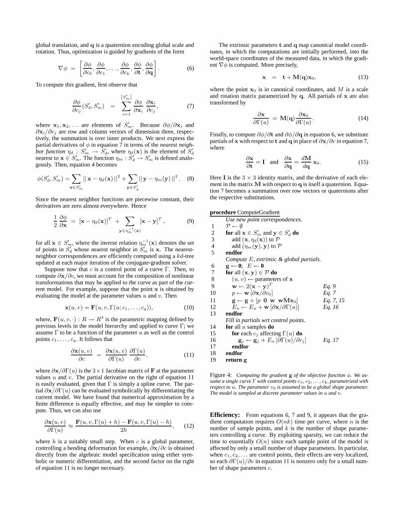
procedureComputeGradientUse new point correspondences.
1 P ← ∅2 for all x ∈ S′m andy ∈ S′d do3 add(x, ηd(x)) toP4 add(ηm(y),y) toP5 endfor
ComputeE, extrinsic & global partials.6 g← 0; E ← 07 for all (x,y) ∈ P do8 (u, v)← parameters ofx9 w← 2(x− y)T Eq. 910 p←w [∂x/∂c0] Eq. 711 g← g + [p 0 w wMx0] Eq. 7, 1512 Eu ← Eu + w [∂x/∂Γ(u)] Eq. 1613 endfor
Fill in partials wrt control points.14 for all u samplesdo15 for eachcj affectingΓ(u) do16 gj ← gj + Eu [∂Γ(u)/∂cj ] Eq. 1717 endfor18 endfor19 return g
Figure 4: Computing the gradientg of the objective functionφ. We as-sume a single curveΓ with control pointsc1, c2, . . . ,ck, parametrized withrespect tou. The parameterc0 is assumed to be a global shape parameter.The model is sampled at discrete parameter values inu andv.
Efficiency: From equations 6, 7 and 9, it appears that the gra-dient computation requiresO(nk) time per curve, wheren is thenumber of sample points, andk is the number of shape parame-ters controlling a curve. By exploiting sparsity, we can reduce thetime to essentiallyO(n) since each sample point of the model isaffected by only a small number of shape parameters. In particular,whenc1, c2, . . . are control points, their effects are very localized,so each∂Γ(u)/∂c in equation 11 is nonzero only for a small num-ber of shape parametersc.
−1 −0.8 −0.6 −0.4 −0.2 0 0.2 0.4 0.6 0.8 1−0.25
−0.2
−0.15
−0.1
−0.05
0
0.05
0.1
−1 −0.8 −0.6 −0.4 −0.2 0 0.2 0.4 0.6 0.8 1−0.25
−0.2
−0.15
−0.1
−0.05
0
0.05
−1 −0.8 −0.6 −0.4 −0.2 0 0.2 0.4 0.6 0.8 10
2
4
6
8
10
12
14
16
18
20
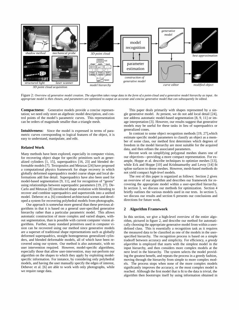
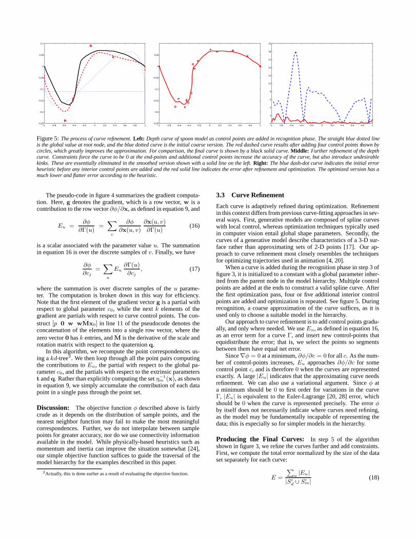
Figure 5:The process of curve refinement.Left: Depth curve of spoon model as control points are added in recognition phase. The straight blue dotted lineis the global value at root node, and the blue dotted curve is the initial coarse version. The red dashed curve results after adding four control points shown bycircles, which greatly improves the approximation. For comparison, the final curve is shown by a black solid curve.Middle: Further refinement of the depthcurve. Constraints force the curve to be0 at the end-points and additional control points increase the accuracy of the curve, but also introduce undesirablekinks. These are essentially eliminated in the smoothed version shown with a solid line on the left.Right: The blue dash-dot curve indicates the initial errorheuristic before any interior control points are added and the red solid line indicates the error after refinement and optimization. The optimized version has amuch lower and flatter error according to the heuristic.
The pseudo-code in figure 4 summarizes the gradient computa-tion. Here,g denotes the gradient, which is a row vector,w is acontribution to the row vector∂φ/∂x, as defined in equation 9, and
Eu =∂φ
∂Γ(u)=∑v
∂φ
∂x(u, v)
∂x(u, v)
∂Γ(u)(16)
is a scalar associated with the parameter valueu. The summationin equation 16 is over the discrete samples ofv. Finally, we have
∂φ
∂cj=∑u
Eu∂Γ(u)
∂cj, (17)
where the summation is over discrete samples of theu parame-ter. The computation is broken down in this way for efficiency.Note that the first element of the gradient vectorg is a partial withrespect to global parameterc0, while the nextk elements of thegradient are partials with respect to curve control points. The con-struct [p 0 w wMx0] in line 11 of the pseudocode denotes theconcatenation of the elements into a single row vector, where thezero vector0 hask entries, andM is the derivative of the scale androtation matrix with respect to the quaternionq.
In this algorithm, we recompute the point correspondences us-ing akd-tree2. We then loop through all the point pairs computingthe contributions toEu, the partial with respect to the global pa-rameterc0, and the partials with respect to the extrinsic parameterst andq. Rather than explicitly computing the setη−1
m (x), as shownin equation 9, we simply accumulate the contribution of each datapoint in a single pass through the point set.
Discussion: The objective functionφ described above is fairlycrude as it depends on the distribution of sample points, and thenearest neighbor function may fail to make the most meaningfulcorrespondences. Further, we do not interpolate between samplepoints for greater accuracy, nor do we use connectivity informationavailable in the model. While physically-based heuristics such asmomentum and inertia can improve the situation somewhat [24],our simple objective function suffices to guide the traversal of themodel hierarchy for the examples described in this paper.
2Actually, this is done earlier as a result of evaluating the objective function.
3.3 Curve Refinement
Each curve is adaptively refined during optimization. Refinementin this context differs from previous curve-fitting approaches in sev-eral ways. First, generative models are composed of spline curveswith local control, whereas optimization techniques typically usedin computer vision entail global shape parameters. Secondly, thecurves of a generative model describe characteristics of a 3-D sur-face rather than approximating sets of 2-D points [17]. Our ap-proach to curve refinement most closely resembles the techniquesfor optimizing trajectories used in animation [4, 20].
When a curve is added during the recognition phase in step 3 offigure 3, it is initialized to a constant with a global parameter inher-ited from the parent node in the model hierarchy. Multiple controlpoints are added at the ends to construct a valid spline curve. Afterthe first optimization pass, four or five additional interior controlpoints are added and optimization is repeated. See figure 5. Duringrecognition, a coarse approximation of the curve suffices, as it isused only to choose a suitable model in the hierarchy.
Our approach to curve refinement is to add control points gradu-ally, and only where needed. We useEu, as defined in equation 16,as an error term for a curveΓ, and insert new control-points thatequidistribute the error; that is, we select the points so segmentsbetween them have equal net error.
Since∇φ = 0 at a minimum,∂φ/∂c = 0 for all c. As the num-ber of control-points increases,Eu approaches∂φ/∂c for somecontrol pointc, and is therefore0 when the curves are representedexactly. A large|Eu| indicates that the approximating curve needsrefinement. We can also use a variational argument. Sinceφ ata minimum should be0 to first order for variations in the curveΓ, |Eu| is equivalent to the Euler-Lagrange [20, 28] error, whichshould be0 when the curve is represented precisely. The errorφby itself does not necessarily indicate where curves need refining,as the model may be fundamentally incapable of representing thedata; this is especially so for simpler models in the hierarchy.
Producing the Final Curves: In step 5 of the algorithmshown in figure 3, we refine the curves further and add constraints.First, we compute the total error normalized by the size of the dataset separately for each curve:
E =
∑u|Eu|
|S′d ∪ S′m|(18)
Based on this total error, we calculate the number of control-pointswe wish to add to each curve using the heuristic
Nc =E
ε, (19)
which adds one control point for eachε of error. We have foundthat a value ofε = 10−3 is suitable for objects of unit dimensions.The control points are again added to equidistribute the error. Then,user-specified constraints such as curve end conditions are added.Refer to the middle of figure 5 for an example. The objective func-tion is minimized again to yield a high-accuracy solution satisfyingthe constraints.
In the final stage, step 6 in figure 3, we ensure that noise in thedata does not lead to extraneous kinks in the model. We do this byintroducing a penalty based on the integrated curvatureβ given by
β =
∫u
|κ(u)| du, (20)
whereκ(u) is the curvature ofΓ at the parameter valueu. We esti-mateβ using numerical quadrature and approximate the derivativesof β with respect to the curve control points using finite differences.These values are summed over all curves in the model. The objec-tive function is then augmented with an extra term
φ = φ+ aβ, (21)
wherea is a positive weight chosen so that the smoothness termand the original objective function are of approximately the samemagnitude. Thus,
a = Kφ0
β0, (22)
where the subscript0 denotes the value after step 5 in the algorithmframework, but before optimizing with respect to the augmentedobjective function. Here,K is a constant that controls the relativeimportance of the two terms, which was fixed at 10 in our tests.
4 Model Hierarchies Used
This section briefly reviews the model hierarchies used in our ex-periments. The hierarchy for the spoon is patterned after the modelgiven by Snyder [21, p. 83]. The generative modeling equation is
spoon(u, v) =
sx(v)
arcx(sy(v),dy(v), u)
by(v) + arcy(sy(v),dy(v), u)
,wheres is the width or shape curve,d is the depth curve, andbis the bend, parametrized sosx = dx = bx. arc(a, b, u) definesa parametric arc passing through(−a, 0), (0, b), and(a, 0) in thexy-pane. The above equation is obtained at the deepest level of thehierarchy, regardless of the path, since all the operators commute.In the root model,s andd are global parameters andb is 0. Asmore complex models are reached, these constants are replaced bycurves. Curves are constrained for this model so thats andd are 0at the end-points, wheres is also perpendicular to thex-axis; sincethe model is symmetric about thex-axis, this last constraint avoidsintroducing a kink. To complete the representation, we also requirea thickness. Since the thickness is typically small and difficult todiscern from range data, we use a constant value derived from theprojection of the acquired data in theyz-plane.
For a ladle-like shape, the arcs are translated by the bend onlyafter first rotating them about they-axis by an angle equal to that ofthe bend curve from the horizontal. This forces the arcs to remainperpendicular to the bend curve. A shape suitable for a cup handleis obtained by making the circular cross-sectionarc rectangular.3
We also used arotating generalized cylinder—the “banana”model defined by Snyder [21, p. 69]—to represent many differ-ent objects. This model rotates a cross-section while scaling andtranslating it, and generalizes common primitives in computer vi-sion known as profile products or simple homogeneous generalizedcylinders. The parametric equation is
banana(u, v) = yrot(R(v))
S(v) Cx(u)
S(v) Cy(u)
Z(v)
whereyrot(θ) is a rotation ofθ about they-axis,R is the para-metric rotation angle,S the scale, andC the 2D cross-section. Theroot model is a right circular cylinder with unit radius and no ro-tation. The curvesR, S, andC are added at more complex levelsin the hierarchy. This class of models can also be used to representsurfaces of revolution, such as the bowl example that is shown.
As the previous model hierarchy demonstrates, our approachsubsumes some common primitives used in computer vision suchas simple homogeneous generalized cylinders. We have also recov-ered globally deformed superquadrics with our approach.
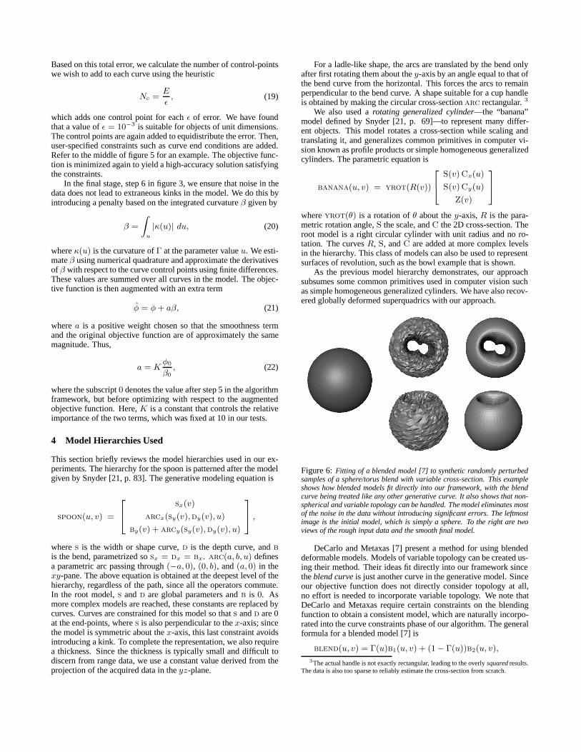
Figure 6:Fitting of a blended model [7] to synthetic randomly perturbedsamples of a sphere/torus blend with variable cross-section. This exampleshows how blended models fit directly into our framework, with the blendcurve being treated like any other generative curve. It also shows that non-spherical and variable topology can be handled. The model eliminates mostof the noise in the data without introducing significant errors. The leftmostimage is the initial model, which is simply a sphere. To the right are twoviews of the rough input data and the smooth final model.
DeCarlo and Metaxas [7] present a method for using blendeddeformable models. Models of variable topology can be created us-ing their method. Their ideas fit directly into our framework sincetheblend curveis just another curve in the generative model. Sinceour objective function does not directly consider topology at all,no effort is needed to incorporate variable topology. We note thatDeCarlo and Metaxas require certain constraints on the blendingfunction to obtain a consistent model, which are naturally incorpo-rated into the curve constraints phase of our algorithm. The generalformula for a blended model [7] is
blend(u, v) = Γ(u)b1(u, v) + (1− Γ(u))b2(u, v),
3The actual handle is not exactly rectangular, leading to the overlysquaredresults.The data is also too sparse to reliably estimate the cross-section from scratch.
whereΓ is the blending curve that can be treated just as any othercurve in the generative model. Hereb1 and b2 are simply con-stituents of the generative model, which can be any shape at all, in-cluding as a special case, the superquadrics and supertoroids usedin [7]. Figure 6 shows an example of recovering blended modelswith our approach.
Although this paper deals primarily with shapes that can be rep-resented by a single generative model, we have carried out someexperiments on simple articulated objects. The watering-can infigure 1 was modeled by first manually segmenting it into body,handle and spout, and then fitting a rotating generalized cylinderto each part. Minor imperfections are primarily due to errors insegmentation. We may also define a single composite generativemodel by combining existing parts, each controlled by separate ex-trinsic and intrinsic parameters. The cup in figure 1 is an example.If the extrinsic transformations of the individual parts are left free—and not constrained to ensure correct connectivity—the user mayneed to make some minor adjustments at the end to ensure the partsconnect properly. While the user-supplied initial guess function canstill be crude, it needs to be more accurate for an articulated objectsince a data point can otherwise be incorrectly associated with thewrong model part.
5 Results
Parameters: For our tests, the complexity constantQ definedbelow equation 1 was set to a deviation of.01 after scaling themodels to have a major axis range from−1 to +1. Thus,Q cor-responds to a percentage error of approximately.5%. The resultsdemonstrate that the algorithm is not very sensitive to the precisevalue ofQ. We report the percentage error using a64×64 tessella-tion of the model. For illustrative purposes only, both range imagesand the model were meshed to create the final images for displayand colors are artificial. Snyder [21] describes alternate methods toimage generative models without mesh creation, but at the cost ofloss of interactivity.
Data: The range data used in our experiments was obtained froma variety of sources. Of the objects in figure 7, the spoon and bowldata are single range images obtained using structured light [25],while 6 cylindrical scans are aligned for the cup data. The ladleis a single range image obtained using the method of Bouguet andPerona [2]. Data for the banana and candle-holder were obtainedusing a mechanical probe, and the watering-can data is a cylindri-cal scan obtained from a laser range-scanner. For the data obtainedfrom the probe, connectivity information was not available, so themeshes for the figures were obtained using the approach of Hoppeet al. [12]. Our algorithm operated directly on the range data, andthe results demonstrate the benefit of recovering a model as op-posed to a mesh, especially in cases of noisy and incomplete data.
Recognition Trees: Figure 8 shows recognition trees for twoobjects—a spoon acquired using structured light, and synthetic datafor a banana-like object. Data on errors are given in figure 9. Theroot models are trivial, and the user-supplied initial guess func-tions need not specify accurate initial estimates; nonetheless thealgorithm is able tobootstrapitself to produce an accurate finalmodel. Paths that are not ultimately selected can sometimes pro-duce strange and interesting results as a curve is trying to adjustto match data that it is incapable of matching. This effect will beespecially noted in the tree for the banana.
Accuracy and Robustness: A visual comparison indicatesthat the method produces a good match to the data, even when the
data is noisy and/or incomplete. As a confirmation of the accuracyof the method, on the synthetic data of the banana shown in fig-ure 8, the technique produces results accurate to within.4%. Asshown in the left of figure 10, even if the input hierarchy is unableto adequately represent the object, the algorithm does the best itcan, producing a simple model that conveys some of the dominantaspects of the shapes.
Finally, we demonstrate the robustness of the technique by run-ning it on a sparse sampling of the spoon data; after removing90%of the spoon data, a visually appealing reasonably accurate modelis still obtained as shown in figure 9.
Compactness: Our models typically had fewer than a hundredparameters, primarily curve control points. This is at least two or-ders of magnitude smaller than the corresponding meshes.
Editing: An example of editing a recovered spoon model into aladle-like shape is shown on the right of figure 10, demonstratinghow easily new models can be constructed by simple and intuitivecurve editing from shapes already recovered.
Computation Time: The entire algorithm took between 20and 30 minutes on a 150 MHz SGI MIPS R4400, depending onmodel complexity and the size of the data set. Each iteration ofthe conjugate gradient took 1-2 seconds, with each optimizationpass taking about 50 iterations. The process was entirely automatic;no manual intervention was required. The total number of points(range data and tessellated model) was typically about15000.
6 Conclusions and Future Work
We have presented a new method for creating concise generativemodels from incomplete range data, given a user-supplied modelhierarchy. Advantages of our approach are simplicity, robustness tonoise, and creation of an intuitive compact model. We extend tradi-tional computer vision algorithms for recovery of specific shapes inthat curves of a user-supplied generative model are estimated; theuser can supply a model of their choice and immediately obtain anautomatic recovery algorithm.
Our work currently has many limitations. The fits obtained arenot perfect, especially when the model inadequately describes thereal object. Even for the synthetic banana-like data used in fig-ure 8, there is some residual error. Our method also does not pre-serve local detail, and there may be artifacts from under- or over-smoothing, such as the squaring near the ends of the spoon model.Further, the algorithm requires the user to specify an appropriatemodel hierarchy, and currently does not allow different hierarchiesto be combined. If the wrong hierarchy is input, a simple modelthat mimics the original to the extent possible will be output asshown on the left of figure 10, but those results may not always beuseful. Also, while the models shown are complex compared tosingle parametric models previously used in computer vision, theyare still fairly simple for graphics as we do not provide automaticsegmentation for recovery of complex articulated objects.
Solving the above problems defines some important directionsfor future work. Improvements could also be made in using morecomplex objective functions and minimization algorithms, moreflexible tradeoffs between accuracy and simplicity, and more ex-haustive non-greedy methods for traversing the input hierarchy. Fi-nally, the model hierarchy used could be learned from examples orcreated automatically from a model database.
While many challenges remain, we believe that algorithms forrecovering high-level models are an important direction of researchfor both computer vision and computer graphics.
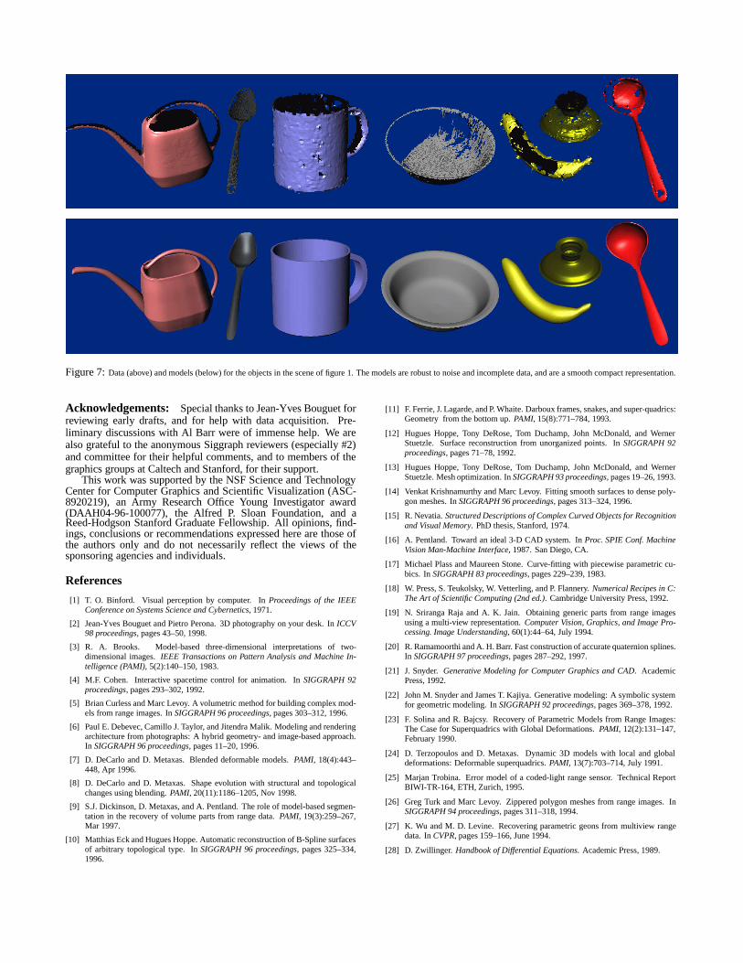
Figure 7:Data (above) and models (below) for the objects in the scene of figure 1. The models are robust to noise and incomplete data, and are a smooth compact representation.
Acknowledgements: Special thanks to Jean-Yves Bouguet forreviewing early drafts, and for help with data acquisition. Pre-liminary discussions with Al Barr were of immense help. We arealso grateful to the anonymous Siggraph reviewers (especially #2)and committee for their helpful comments, and to members of thegraphics groups at Caltech and Stanford, for their support.
This work was supported by the NSF Science and TechnologyCenter for Computer Graphics and Scientific Visualization (ASC-8920219), an Army Research Office Young Investigator award(DAAH04-96-100077), the Alfred P. Sloan Foundation, and aReed-Hodgson Stanford Graduate Fellowship. All opinions, find-ings, conclusions or recommendations expressed here are those ofthe authors only and do not necessarily reflect the views of thesponsoring agencies and individuals.
References
[1] T. O. Binford. Visual perception by computer. InProceedings of the IEEEConference on Systems Science and Cybernetics, 1971.
[2] Jean-Yves Bouguet and Pietro Perona. 3D photography on your desk. InICCV98 proceedings, pages 43–50, 1998.
[3] R. A. Brooks. Model-based three-dimensional interpretations of two-dimensional images.IEEE Transactions on Pattern Analysis and Machine In-telligence (PAMI), 5(2):140–150, 1983.
[4] M.F. Cohen. Interactive spacetime control for animation. InSIGGRAPH 92proceedings, pages 293–302, 1992.
[5] Brian Curless and Marc Levoy. A volumetric method for building complex mod-els from range images. InSIGGRAPH 96 proceedings, pages 303–312, 1996.
[6] Paul E. Debevec, Camillo J. Taylor, and Jitendra Malik. Modeling and renderingarchitecture from photographs: A hybrid geometry- and image-based approach.In SIGGRAPH 96 proceedings, pages 11–20, 1996.
[7] D. DeCarlo and D. Metaxas. Blended deformable models.PAMI, 18(4):443–448, Apr 1996.
[8] D. DeCarlo and D. Metaxas. Shape evolution with structural and topologicalchanges using blending.PAMI, 20(11):1186–1205, Nov 1998.
[9] S.J. Dickinson, D. Metaxas, and A. Pentland. The role of model-based segmen-tation in the recovery of volume parts from range data.PAMI, 19(3):259–267,Mar 1997.
[10] Matthias Eck and Hugues Hoppe. Automatic reconstruction of B-Spline surfacesof arbitrary topological type. InSIGGRAPH 96 proceedings, pages 325–334,1996.
[11] F. Ferrie, J. Lagarde, and P. Whaite. Darboux frames, snakes, and super-quadrics:Geometry from the bottom up.PAMI, 15(8):771–784, 1993.
[12] Hugues Hoppe, Tony DeRose, Tom Duchamp, John McDonald, and WernerStuetzle. Surface reconstruction from unorganized points. InSIGGRAPH 92proceedings, pages 71–78, 1992.
[13] Hugues Hoppe, Tony DeRose, Tom Duchamp, John McDonald, and WernerStuetzle. Mesh optimization. InSIGGRAPH 93 proceedings, pages 19–26, 1993.
[14] Venkat Krishnamurthy and Marc Levoy. Fitting smooth surfaces to dense poly-gon meshes. InSIGGRAPH 96 proceedings, pages 313–324, 1996.
[15] R. Nevatia.Structured Descriptions of Complex Curved Objects for Recognitionand Visual Memory. PhD thesis, Stanford, 1974.
[16] A. Pentland. Toward an ideal 3-D CAD system. InProc. SPIE Conf. MachineVision Man-Machine Interface, 1987. San Diego, CA.
[17] Michael Plass and Maureen Stone. Curve-fitting with piecewise parametric cu-bics. InSIGGRAPH 83 proceedings, pages 229–239, 1983.
[18] W. Press, S. Teukolsky, W. Vetterling, and P. Flannery.Numerical Recipes in C:The Art of Scientific Computing (2nd ed.). Cambridge University Press, 1992.
[19] N. Sriranga Raja and A. K. Jain. Obtaining generic parts from range imagesusing a multi-view representation.Computer Vision, Graphics, and Image Pro-cessing. Image Understanding, 60(1):44–64, July 1994.
[20] R. Ramamoorthi and A. H. Barr. Fast construction of accurate quaternion splines.In SIGGRAPH 97 proceedings, pages 287–292, 1997.
[21] J. Snyder.Generative Modeling for Computer Graphics and CAD. AcademicPress, 1992.
[22] John M. Snyder and James T. Kajiya. Generative modeling: A symbolic systemfor geometric modeling. InSIGGRAPH 92 proceedings, pages 369–378, 1992.
[23] F. Solina and R. Bajcsy. Recovery of Parametric Models from Range Images:The Case for Superquadrics with Global Deformations.PAMI, 12(2):131–147,February 1990.
[24] D. Terzopoulos and D. Metaxas. Dynamic 3D models with local and globaldeformations: Deformable superquadrics.PAMI, 13(7):703–714, July 1991.
[25] Marjan Trobina. Error model of a coded-light range sensor. Technical ReportBIWI-TR-164, ETH, Zurich, 1995.
[26] Greg Turk and Marc Levoy. Zippered polygon meshes from range images. InSIGGRAPH 94 proceedings, pages 311–318, 1994.
[27] K. Wu and M. D. Levine. Recovering parametric geons from multiview rangedata. InCVPR, pages 159–166, June 1994.
[28] D. Zwillinger. Handbook of Differential Equations. Academic Press, 1989.

Shape Depth Bend
Spoon
B
0S D B
S
After Smoothing (Final Model)
Refine
Root Input Data
Refined Model
B Depth + BendShape + Depth
3
1
2
Cross SectionC
Root (Cylinder)
SR
Refined ModelAfter Smoothing (Final Model)
Refine
Original Input Data
ScaleRotation
C S
C
Banana
Cross Section Rotation + Scale Rotation +
Figure 8:Recognition trees for the spoon (left) and banana (right). Highlighted nodes (lighter background) indicate the best guess at some level, and only nodes reachable from ahighlighted node are generated. The algorithm is able tobootstrapitself, starting from very crude initial conditions, improving at each stage and finishing with an accurate model.
D
C
D
C2.43
D
C
1.93
ROOT
2.562.56
C
D
DEPTH
REFINED
C
D
C
D 0.51
SPOON
SMOOTH
1.60
0.60
1.51
B
1.53
BEND
1.79
1.29
SHAPE
2.03BS
B
D
S
2.23
1.23
C
D
B+D
C
D
D
C 1.61
0.61
S+D
0.54
S+D+B
2.04
0.34
REFINED
C 1.34
S
D
1.35
0.35C
D
SMOOTH
BANANA
R
ROOT (CYL)
4.714.71
CS
4.02
3.52
Cross-Section
C
C
D
C
D
C
SCALE
4.00
3.50C
1.85C
D
C
D 1.85
ROTATION
2.35
D D
1.87
C 1.52
0.52
R+S
0.37
C+R
2.85
C+R+S
D
C
Figure 9:Left: Percentage deviation errors (D) and total costs (C) for the spoon (left) and banana (right).Middle: Fitting of model to very sparse data. On top is a pointcloudwith fewer than 900 points. The middle shows the recovered model while the bottom is a mesh obtained from Hoppe’s [12] algorithm on the same data. A comparison indicates therobustness of our approach.Right: The top shows a superquadric fit to the banana data while the bottom shows our model, indicating the benefit of generative models.
−1 −0.8 −0.6 −0.4 −0.2 0 0.2 0.4 0.6 0.8 10
0.05
0.1
0.15
0.2
0.25
0.3
0.35
−1 −0.8 −0.6 −0.4 −0.2 0 0.2 0.4 0.6 0.8 1−0.3
−0.25
−0.2
−0.15
−0.1
−0.05
0
0.05
0.1
Figure 10:Left: Models recovered using a model hierarchy that was a poor match for the actual data since it did not possess the appropriate degrees of freedom to adequatelyrepresent the object. The two objects on the left are the banana and bowl recovered using the spoon hierarchy, while the two objects on the right are the ladle and spoon recoveredusing the rotating generalized cylinder hierarchy. The algorithm did the best that it could, and managed to convey some of the dominant aspects of the shapes.Middle: Editing arecovered spoon model into a ladle. Only a few control points need to be moved to get a radically different shape.Middle Top: Edited shape curve before (blue) and after (red)editing. Control points are shown as circles.Middle Bottom:A similar plot for the depth curve.Right: A view of the edited model.