Creating synthetic discrete-response regression modelsageconsearch.umn.edu/bitstream/152284/2/sjart_st0186.pdf · Creating synthetic discrete-response regression models ... negative

The Stata Journal (2010)10, Number 1, pp. 104–124

Creating synthetic discrete-response regression

models

Joseph M. HilbeArizona State University

and Jet Propulsion Laboratory, [email protected]

Abstract. The development and use of synthetic regression models has provento assist statisticians in better understanding bias in data, as well as how to bestinterpret various statistics associated with a modeling situation. In this article, Ipresent code that can be easily amended for the creation of synthetic binomial,count, and categorical response models. Parameters may be assigned to any num-ber of predictors (which are shown as continuous, binary, or categorical), negativebinomial heterogeneity parameters may be assigned, and the number of levels orcut points and values may be specified for ordered and unordered categorical re-sponse models. I also demonstrate how to introduce an offset into synthetic dataand how to test synthetic models using Monte Carlo simulation. Finally, I intro-duce code for constructing a synthetic NB2-logit hurdle model.

Keywords: st0186, synthetic, pseudorandom, Monte Carlo, simulation, logistic,probit, Poisson, NB1, NB2, NB-C, hurdle, offset, ordered, multinomial

1 Introduction

Statisticians use synthetic datasets to evaluate the appropriateness of fit statistics andto determine the effect of modeling after making specific alterations to the data. Modelsbased on synthetically created datasets have proved to be extremely useful in this respectand appear to be used with increasing frequency in texts on statistical modeling.

In this article, I demonstrate how to construct synthetic datasets that are appropri-ate for various popular discrete-response regression models. The same methods may beused to create data specific to a wide variety of alternative models. In particular, I showhow to create synthetic datasets for given types of binomial, Poisson, negative binomial,proportional odds, multinomial, and hurdle models using Stata’s pseudorandom-numbergenerators. I demonstrate standard models, models with an offset, and models havinguser-defined binary, factor, or nonrandom continuous predictors. Typically, syntheticmodels have predictors with values distributed as pseudorandom uniform or pseudoran-dom normal. This will be our paradigm case, but synthetic datasets do not have to beestablished in such a manner—as I demonstrate.

In 1995, Walter Linde-Zwirble and I developed several pseudorandom-number gen-erators using Stata’s programming language (Hilbe and Linde-Zwirble 1995, 1998), in-cluding the binomial, Poisson, negative binomial, gamma, inverse Gaussian, beta bino-mial, and others. Based on the rejection method, random numbers that were based on

c© 2010 StataCorp LP st0186

J. M. Hilbe 105

distributions belonging to the one-parameter exponential family of distributions couldrather easily be manipulated to generate full synthetic datasets. A synthetic binomialdataset could be created, for example, having randomly generated predictors with cor-responding user-specified parameters and denominators. One could also specify whetherthe data was to be logit, probit, or any other appropriate binomial link function.

Stata’s pseudorandom-number generators are not only based on a different methodfrom those used in the earlier rnd* suite of generators but also, in general, use differentparameters. The examples in this article all rely on the new Stata functions and aretherefore unlike model creation using the older programs. This is particularly the casefor the negative binomial.

I divide this article into four sections. First, I discuss creation of synthetic countresponse models—specifically, Poisson, log-linked negative binomial (NB2), linear nega-tive binomial (NB1), and canonical negative binomial (NB-C) models. Second, I developcode for binomial models, which include both Bernoulli or binary models and binomialor grouped logit and probit models. Because the logic of creating and extending suchmodels was developed in the preceding section on count models, I do not spend muchtime explaining how these models work. The third section provides a relatively briefoverview of creating synthetic proportional slopes models, including the proportionalodds model, and code for constructing synthetic categorical response models, e.g., themultinomial logit. Finally, I present code on how to develop synthetic hurdle models,which are examples of two-part models having binary and count components. Statis-ticians should find it relatively easy to adjust the code that is provided to constructsynthetic data and models for other discrete-response regression models.

2 Synthetic count models

I first create a simple Poisson model because Stata’s rpoisson() function is similar tomy original rndpoi (used to create a single vector of Poisson-distributed numbers witha specified mean) and rndpoix (used to create a Poisson dataset) commands. Uniformrandom variates work as well as and at times superior to random normal variates for thecreation of continuous predictors, which are used to create many of the models below.The mean of the resultant fitted value will be lower using the uniform distribution, butthe model results are nevertheless identical.

(Continued on next page)

106 Creating synthetic discrete-response regression models

* SYNTHETIC POISSON DATA* [With predictors x1 and x2, having respective parameters of 0.75 and -1.25* and an intercept of 2]* poi_rng.do 22Jan2009clearset obs 50000set seed 4744generate x1 = invnormal(runiform()) // normally distributed: values between

// ~ -4.5 - 4.5generate x2 = invnormal(runiform()) // normally distributed: values between

// ~ -4.5 - 4.5generate xb = 2 + 0.75*x1 - 1.25*x2 // linear predictor; define parametersgenerate exb = exp(xb) // inverse link; define Poisson meangenerate py = rpoisson(exb) // generate random Poisson variate with mean=exbglm py x1 x2, nolog family(poi) // model resultant data

The model output is given as

. glm py x1 x2, nolog family(poi)

Generalized linear models No. of obs = 50000Optimization : ML Residual df = 49997

Scale parameter = 1Deviance = 52295.46204 (1/df) Deviance = 1.045972Pearson = 50078.33993 (1/df) Pearson = 1.001627

Variance function: V(u) = u [Poisson]Link function : g(u) = ln(u) [Log]

AIC = 4.783693Log likelihood = -119589.3262 BIC = -488661

OIMpy Coef. Std. Err. z P>|z| [95% Conf. Interval]

x1 .7488765 .0009798 764.35 0.000 .7469562 .7507967x2 -1.246898 .0009878 -1262.27 0.000 -1.248834 -1.244962

_cons 2.002672 .0017386 1151.91 0.000 1.999265 2.00608

Notice that the parameter estimates approximate the user-defined values. If wedelete the seed line, add code to store each parameter estimate, and convert the do-fileto an r-class ado-file, it is possible to perform a Monte Carlo simulation of the syntheticmodel parameters. The above synthetic Poisson data and model code may be amendedto do a simple Monte Carlo simulation as follows:

J. M. Hilbe 107

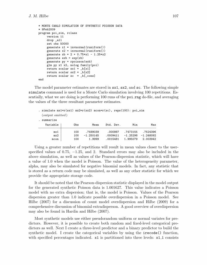
* MONTE CARLO SIMULATION OF SYNTHETIC POISSON DATA* 9Feb2009program poi_sim, rclass

version 11drop _allset obs 50000generate x1 = invnormal(runiform())generate x2 = invnormal(runiform())generate xb = 2 + 0.75*x1 - 1.25*x2generate exb = exp(xb)generate py = rpoisson(exb)glm py x1 x2, nolog family(poi)return scalar sx1 = _b[x1]return scalar sx2 = _b[x2]return scalar sc = _b[_cons]

end

The model parameter estimates are stored in sx1, sx2, and sc. The following simplesimulate command is used for a Monte Carlo simulation involving 100 repetitions. Es-sentially, what we are doing is performing 100 runs of the poi rng do-file, and averagingthe values of the three resultant parameter estimates.

. simulate mx1=r(sx1) mx2=r(sx2) mcon=r(sc), reps(100): poi_sim

(output omitted )

. summarize

Variable Obs Mean Std. Dev. Min Max

mx1 100 .7499039 .000987 .7473155 .7524396mx2 100 -1.250145 .0009411 -1.25298 -1.248092

mcon 100 1.9999 .0015481 1.995079 2.003942

Using a greater number of repetitions will result in mean values closer to the user-specified values of 0.75, −1.25, and 2. Standard errors may also be included in theabove simulation, as well as values of the Pearson-dispersion statistic, which will havea value of 1.0 when the model is Poisson. The value of the heterogeneity parameter,alpha, may also be simulated for negative binomial models. In fact, any statistic thatis stored as a return code may be simulated, as well as any other statistic for which weprovide the appropriate storage code.

It should be noted that the Pearson-dispersion statistic displayed in the model outputfor the generated synthetic Poisson data is 1.001627. This value indicates a Poissonmodel with no extra dispersion; that is, the model is Poisson. Values of the Pearsondispersion greater than 1.0 indicate possible overdispersion in a Poisson model. SeeHilbe (2007) for a discussion of count model overdispersion and Hilbe (2009) for acomprehensive discussion of binomial extradisperson. A good overview of overdispersionmay also be found in Hardin and Hilbe (2007).

Most synthetic models use either pseudorandom uniform or normal variates for pre-dictors. However, it is possible to create both random and fixed-level categorical pre-dictors as well. Next I create a three-level predictor and a binary predictor to build thesynthetic model. I create the categorical variables by using the irecode() function,with specified percentages indicated. x1 is partitioned into three levels: x1 1 consists


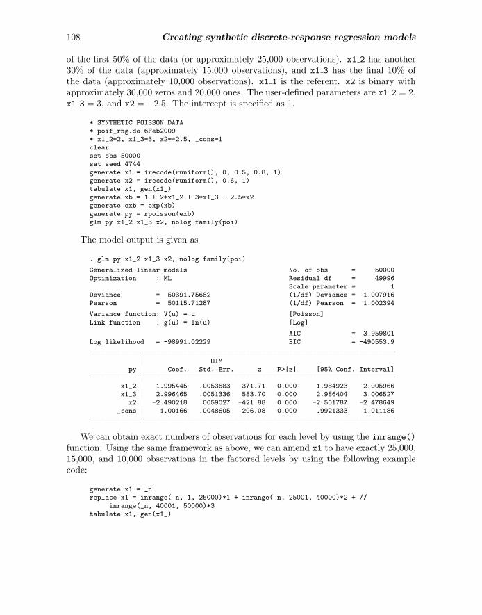
of the first 50% of the data (or approximately 25,000 observations). x1 2 has another30% of the data (approximately 15,000 observations), and x1 3 has the final 10% ofthe data (approximately 10,000 observations). x1 1 is the referent. x2 is binary withapproximately 30,000 zeros and 20,000 ones. The user-defined parameters are x1 2 = 2,x1 3 = 3, and x2 = −2.5. The intercept is specified as 1.

* SYNTHETIC POISSON DATA* poif_rng.do 6Feb2009* x1_2=2, x1_3=3, x2=-2.5, _cons=1clearset obs 50000set seed 4744generate x1 = irecode(runiform(), 0, 0.5, 0.8, 1)generate x2 = irecode(runiform(), 0.6, 1)tabulate x1, gen(x1_)generate xb = 1 + 2*x1_2 + 3*x1_3 - 2.5*x2generate exb = exp(xb)generate py = rpoisson(exb)glm py x1_2 x1_3 x2, nolog family(poi)


. glm py x1_2 x1_3 x2, nolog family(poi)


Scale parameter = 1Deviance = 50391.75682 (1/df) Deviance = 1.007916Pearson = 50115.71287 (1/df) Pearson = 1.002394


AIC = 3.959801Log likelihood = -98991.02229 BIC = -490553.9


x1_2 1.995445 .0053683 371.71 0.000 1.984923 2.005966x1_3 2.996465 .0051336 583.70 0.000 2.986404 3.006527

x2 -2.490218 .0059027 -421.88 0.000 -2.501787 -2.478649_cons 1.00166 .0048605 206.08 0.000 .9921333 1.011186

We can obtain exact numbers of observations for each level by using the inrange()

function. Using the same framework as above, we can amend x1 to have exactly 25,000,15,000, and 10,000 observations in the factored levels by using the following examplecode:

generate x1 = _nreplace x1 = inrange(_n, 1, 25000)*1 + inrange(_n, 25001, 40000)*2 + //

inrange(_n, 40001, 50000)*3tabulate x1, gen(x1_)

J. M. Hilbe 109

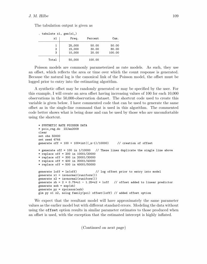
The tabulation output is given as

. tabulate x1, gen(x1_)

x1 Freq. Percent Cum.

1 25,000 50.00 50.002 15,000 30.00 80.003 10,000 20.00 100.00

Total 50,000 100.00

Poisson models are commonly parameterized as rate models. As such, they usean offset, which reflects the area or time over which the count response is generated.Because the natural log is the canonical link of the Poisson model, the offset must belogged prior to entry into the estimating algorithm.

A synthetic offset may be randomly generated or may be specified by the user. Forthis example, I will create an area offset having increasing values of 100 for each 10,000observations in the 50,000-observation dataset. The shortcut code used to create thisvariable is given below. I have commented code that can be used to generate the sameoffset as in the single-line command that is used in this algorithm. The commentedcode better shows what is being done and can be used by those who are uncomfortableusing the shortcut.

* SYNTHETIC RATE POISSON DATA* poio_rng.do 22Jan2009clearset obs 50000set seed 4744generate off = 100 + 100*int((_n-1)/10000) // creation of offset

* generate off = 100 in 1/10000 // These lines duplicate the single line above* replace off = 200 in 10001/20000* replace off = 300 in 20001/30000* replace off = 400 in 30001/40000* replace off = 500 in 40001/50000

generate loff = ln(off) // log offset prior to entry into modelgenerate x1 = invnormal(runiform())generate x2 = invnormal(runiform())generate xb = 2 + 0.75*x1 - 1.25*x2 + loff // offset added to linear predictorgenerate exb = exp(xb)generate py = rpoisson(exb)glm py x1 x2, nolog family(poi) offset(loff) // added offset option

We expect that the resultant model will have approximately the same parametervalues as the earlier model but with different standard errors. Modeling the data withoutusing the offset option results in similar parameter estimates to those produced whenan offset is used, with the exception that the estimated intercept is highly inflated.



The results of the rate-parameterized Poisson algorithm above are displayed below:

. glm py x1 x2, nolog family(poi) offset(loff)


Scale parameter = 1Deviance = 49847.73593 (1/df) Deviance = .9970145Pearson = 49835.24046 (1/df) Pearson = .9967646




x1 .7500656 .0000562 1.3e+04 0.000 .7499555 .7501758x2 -1.250067 .0000576 -2.2e+04 0.000 -1.25018 -1.249954

_cons 1.999832 .0001009 2.0e+04 0.000 1.999635 2.00003loff (offset)

I mentioned earlier that a Poisson model having a Pearson dispersion greater than 1.0indicates possible overdispersion. The NB2 model is commonly used in such situationsto accommodate the extra dispersion.

The NB2 parameterization of the negative binomial can be generated as a Poisson-gamma mixture model, with a gamma scale parameter of 1. We use this method tocreate synthetic NB2 data. The negative binomial random-number generator in Statais not parameterized as NB2 but rather derives directly from the NB-C model (see Hilbe[2007]). rnbinomial() may be used to create a synthetic NB-C model, but not NB2 orNB1. Below is code that can be used to construct NB2 model data. The same parametersare used here as for the above Poisson models.

* SYNTHETIC NEGATIVE BINOMIAL (NB2) DATA* nb2_rng.do 22Jan2009clearset obs 50000set seed 8444generate x1 = invnormal(runiform())generate x2 = invnormal(runiform())generate xb = 2 + 0.75*x1 - 1.25*x2 // same linear predictor as Poisson abovegenerate a = .5 // value of alpha, the NB2 heterogeneity

parametergenerate ia = 1/a // inverse alphagenerate exb = exp(xb) // NB2 meangenerate xg = rgamma(ia, a) // generate random gamma variate given alphagenerate xbg = exb*xg // gamma variate parameterized by linear

predictorgenerate nby = rpoisson(xbg) // generate mixture of gamma and Poissonglm nby x1 x2, family(nb ml) nolog // model as negative binomial (NB2)

J. M. Hilbe 111


. glm nby x1 x2, family(nb ml) nolog


Scale parameter = 1Deviance = 54131.21274 (1/df) Deviance = 1.082689Pearson = 49994.6481 (1/df) Pearson = .999953

Variance function: V(u) = u+(.5011)u^2 [Neg. Binomial]Link function : g(u) = ln(u) [Log]


OIMnby Coef. Std. Err. z P>|z| [95% Conf. Interval]

x1 .7570565 .0038712 195.56 0.000 .749469 .764644x2 -1.252193 .0040666 -307.92 0.000 -1.260164 -1.244223

_cons 1.993917 .0039504 504.74 0.000 1.986175 2.00166

Note: Negative binomial parameter estimated via ML and treated as fixed once

The values of the parameters and of alpha closely approximate the values specifiedin the algorithm. These values may of course be altered by the user. Note also thevalues of the dispersion statistics. The Pearson dispersion approximates 1.0, indicatingan approximate “perfect” fit. The deviance dispersion is 8% greater, demonstrating thatit is not to be used as an assessment of overdispersion. In the same manner in whicha Poisson model may be Poisson overdispersed, an NB2 model may be overdispersed aswell. It may, in fact, overadjust for Poisson overdispersion. Scaling standard errors orapplying a robust variance estimate can be used to adjust standard errors in the caseof NB2 overdispersion. See Hilbe (2007) for a discussion of NB2 overdispersion and howit compares with Poisson overdispersion.

If you desire to more critically test the negative binomial dispersion statistic, thenyou should use a Monte Carlo simulation routine. The NB2 negative binomial hetero-geneity parameter, α, is stored in e(a) but must be referred to using single quotes,‘e(a)’. Observe how the remaining statistics we wish to use in the Monte Carlo simu-lation program are stored.

* SIMULATION OF SYNTHETIC NB2 DATA* x1=.75, x2=-1.25, _cons=2, alpha=0.5program nb2_sim, rclassversion 11clearset obs 50000generate x1 = invnormal(runiform()) // define predictorsgenerate x2 = invnormal(runiform())generate xb = 2 + 0.75*x1 - 1.25*x2 // define parameter valuesgenerate a = .5generate ia = 1/agenerate exb = exp(xb)generate xg = rgamma(ia, a)generate xbg = exb*xggenerate nby = rpoisson(xbg)


glm nby x1 x2, nolog family(nb ml)return scalar sx1 = _b[x1] // x1return scalar sx2 = _b[x2] // x2return scalar sxc = _b[_cons] // intercept (_cons)return scalar pd = e(dispers_p) // Pearson dispersionreturn scalar dd = e(dispers_s) // deviance dispersionreturn scalar _a = `e(a)´ // alphaend

To obtain the Monte Carlo averaged statistics we desire, use the following optionswith the simulate command:

. simulate mx1=r(sx1) mx2=r(sx2) mxc=r(sxc) pdis=r(pd) ddis=r(dd) alpha=r(_a),> reps(100): nb2_sim

(output omitted )

. summarize


mx1 100 .750169 .0036599 .7407614 .758591mx2 100 -1.250081 .0037403 -1.258952 -1.240567mxc 100 2.000052 .0040703 1.987038 2.010417

pdis 100 1.000241 .0050856 .9881558 1.01285ddis 100 1.084059 .0015233 1.079897 1.087076

alpha 100 .5001092 .0042068 .4873724 .509136

Note the range of parameter and dispersion values. The code for constructing syn-thetic datasets produces quite good values; i.e., the mean of the parameter estimates isvery close to their respective target values, and the standard errors are tight. This isexactly what we want from an algorithm that creates synthetic data.

We may use an offset into the NB2 algorithm in the same manner as we did for thePoisson. Because the mean of the Poisson and NB2 are both exp(xb), we may use thesame method. The synthetic NB2 data and model with offset is in the nb2o rng.do file.

The NB1 model is also based on a Poisson-gamma mixture distribution. The NB1

heterogeneity or ancillary parameter is typically referred to as δ, not α as with NB2.Converting the NB2 algorithm to NB1 entails defining idelta as the inverse of the valueof delta, the desired value of the model ancillary parameter, multiplying the result by thefitted value, exb. The terms idelta and 1/idelta are given to the rgamma() function.All else is the same as in the NB2 algorithm. The resultant synthetic data are modeledusing Stata’s nbreg command with the disp(constant) option.

J. M. Hilbe 113

* SYNTHETIC LINEAR NEGATIVE BINOMIAL (NB1) DATA* nb1_rng.do 3Apr2006* Synthetic NB1 data and model* x1= 1.1; x2= -.8; x3= .2; _c= .7* delta = .3 (1/.3 = 3.3333333)quietly {

clearset obs 50000set seed 13579generate x1 = invnormal(runiform())generate x2 = invnormal(runiform())generate x3 = invnormal(runiform())generate xb = .7 + 1.1*x1 - .8*x2 + .2*x3generate exb = exp(xb)generate idelta = 3.3333333*exbgenerate xg = rgamma(idelta, 1/idelta)generate xbg = exb*xggenerate nb1y = rpoisson(xbg)

}nbreg nb1y x1 x2 x3, nolog disp(constant)


. nbreg nb1y x1 x2 x3, nolog disp(constant)

Negative binomial regression Number of obs = 49910LR chi2(3) = 82361.44

Dispersion = constant Prob > chi2 = 0.0000Log likelihood = -89323.313 Pseudo R2 = 0.3156

nb1y Coef. Std. Err. z P>|z| [95% Conf. Interval]

x1 1.098772 .0022539 487.49 0.000 1.094354 1.103189x2 -.8001773 .0022635 -353.51 0.000 -.8046137 -.7957409x3 .1993391 .0022535 88.46 0.000 .1949223 .2037559

_cons .7049061 .0038147 184.79 0.000 .6974294 .7123827

/lndelta -1.193799 .029905 -1.252411 -1.135186

delta .3030678 .0090632 .2858147 .3213623

Likelihood-ratio test of delta=0: chibar2(01) = 1763.21 Prob>=chibar2 = 0.000

The parameter values and value of delta closely approximate the specified values.

The NB-C, however, must be constructed in an entirely different manner from NB2,NB1, or Poisson. NB-C is not a Poisson-gamma mixture and is based on the negative bi-nomial probability distribution function. Stata’s rnbinomial(a,b) function can be usedto construct NB-C data. Other options, such as offsets, nonrandom variance adjusters,and so forth, are easily adaptable for the nbc rng.do file.

* SYNTHETIC CANONICAL NEGATIVE BINOMIAL (NB-C) DATA* nbc_rng.do 30dec2005clearset obs 50000set seed 7787generate x1 = runiform()generate x2 = runiform()


generate xb = 1.25*x1 + .1*x2 - 1.5generate a = 1.15generate mu = 1/((exp(-xb)-1)*a) // inverse link functiongenerate p = 1/(1+a*mu) // probabilitygenerate r = 1/agenerate y = rnbinomial(r, p)cnbreg y x1 x2, nolog

I wrote a maximum likelihood NB-C command, cnbreg, in 2005, which was postedto the Statistical Software Components (SSC) site, and I posted an amendment in lateFebruary 2009. The statistical results are the same in the original and the amendedversion, but the amendment is more efficient and pedagogically easier to understand.Rather than simply inserting the NB-C inverse link function in terms of xb for eachinstance of µ in the log-likelihood function, I have reduced the formula for the NB-C loglikelihood to

LLNB−C =∑

[y(xb) + (1/α)ln{1 − exp(xb)} + lnΓ(y + 1/α) − lnΓ(y + 1) − lnΓ(1/α)]

Also posted to the site is a heterogeneous NB-C regression command that allowsparameterization of the heterogeneity parameter, α. Stata calls the NB2 version ofthis a generalized negative binomial. However, as I discuss in Hilbe (2007), there arepreviously implemented generalized negative binomial models with entirely differentparameterizations. Some are discussed in that source. Moreover, LIMDEP has offereda heterogeneous negative binomial for many years that is the same model as is thegeneralized negative binomial in Stata. For these reasons, I prefer labeling Stata’sgnbreg command a heterogeneous model. A hcnbreg command was also posted to SSC

in 2005.

The synthetic NB-C model of the above created data is displayed below. I havespecified values of x1 and x2 as 1.25 and 0.1, respectively, and an intercept value of−1.5. alpha is given as 1.15. The model closely reflects the user-specified parameters.

. cnbreg y x1 x2, nologinitial: log likelihood = -<inf> (could not be evaluated)feasible: log likelihood = -85868.162rescale: log likelihood = -78725.374rescale eq: log likelihood = -71860.156

Canonical Negative Binomial Regression Number of obs = 50000Wald chi2(2) = 6386.70

Log likelihood = -62715.384 Prob > chi2 = 0.0000

y Coef. Std. Err. z P>|z| [95% Conf. Interval]

x1 1.252675 .015776 79.40 0.000 1.221754 1.283595x2 .1009038 .0091313 11.05 0.000 .0830068 .1188008

_cons -1.504659 .0177159 -84.93 0.000 -1.539382 -1.469937

/lnalpha .133643 .0153947 8.68 0.000 .1034699 .1638161

alpha 1.142985 .0175959 1.109012 1.177998

AIC Statistic = 2.509

J. M. Hilbe 115

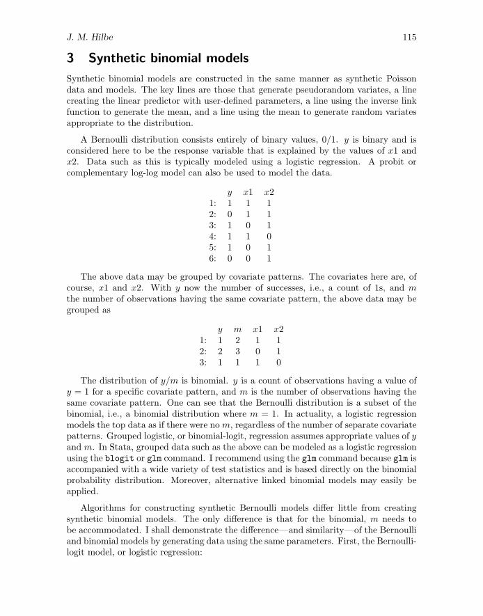
3 Synthetic binomial models

Synthetic binomial models are constructed in the same manner as synthetic Poissondata and models. The key lines are those that generate pseudorandom variates, a linecreating the linear predictor with user-defined parameters, a line using the inverse linkfunction to generate the mean, and a line using the mean to generate random variatesappropriate to the distribution.

A Bernoulli distribution consists entirely of binary values, 0/1. y is binary and isconsidered here to be the response variable that is explained by the values of x1 andx2. Data such as this is typically modeled using a logistic regression. A probit orcomplementary log-log model can also be used to model the data.

y x1 x21: 1 1 12: 0 1 13: 1 0 14: 1 1 05: 1 0 16: 0 0 1

The above data may be grouped by covariate patterns. The covariates here are, ofcourse, x1 and x2. With y now the number of successes, i.e., a count of 1s, and mthe number of observations having the same covariate pattern, the above data may begrouped as

y m x1 x21: 1 2 1 12: 2 3 0 13: 1 1 1 0

The distribution of y/m is binomial. y is a count of observations having a value ofy = 1 for a specific covariate pattern, and m is the number of observations having thesame covariate pattern. One can see that the Bernoulli distribution is a subset of thebinomial, i.e., a binomial distribution where m = 1. In actuality, a logistic regressionmodels the top data as if there were no m, regardless of the number of separate covariatepatterns. Grouped logistic, or binomial-logit, regression assumes appropriate values of yand m. In Stata, grouped data such as the above can be modeled as a logistic regressionusing the blogit or glm command. I recommend using the glm command because glm isaccompanied with a wide variety of test statistics and is based directly on the binomialprobability distribution. Moreover, alternative linked binomial models may easily beapplied.

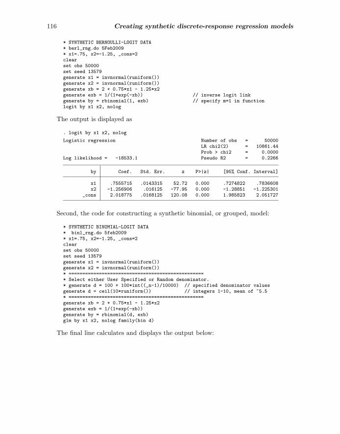
Algorithms for constructing synthetic Bernoulli models differ little from creatingsynthetic binomial models. The only difference is that for the binomial, m needs tobe accommodated. I shall demonstrate the difference—and similarity—of the Bernoulliand binomial models by generating data using the same parameters. First, the Bernoulli-logit model, or logistic regression:


* SYNTHETIC BERNOULLI-LOGIT DATA* berl_rng.do 5Feb2009* x1=.75, x2=-1.25, _cons=2clearset obs 50000set seed 13579generate x1 = invnormal(runiform())generate x2 = invnormal(runiform())generate xb = 2 + 0.75*x1 - 1.25*x2generate exb = 1/(1+exp(-xb)) // inverse logit linkgenerate by = rbinomial(1, exb) // specify m=1 in functionlogit by x1 x2, nolog

The output is displayed as

. logit by x1 x2, nolog

Logistic regression Number of obs = 50000LR chi2(2) = 10861.44Prob > chi2 = 0.0000

Log likelihood = -18533.1 Pseudo R2 = 0.2266

by Coef. Std. Err. z P>|z| [95% Conf. Interval]

x1 .7555715 .0143315 52.72 0.000 .7274822 .7836608x2 -1.256906 .016125 -77.95 0.000 -1.28851 -1.225301

_cons 2.018775 .0168125 120.08 0.000 1.985823 2.051727

Second, the code for constructing a synthetic binomial, or grouped, model:

* SYNTHETIC BINOMIAL-LOGIT DATA* binl_rng.do 5feb2009* x1=.75, x2=-1.25, _cons=2clearset obs 50000set seed 13579generate x1 = invnormal(runiform())generate x2 = invnormal(runiform())* =================================================* Select either User Specified or Random denominator.* generate d = 100 + 100*int((_n-1)/10000) // specified denominator valuesgenerate d = ceil(10*runiform()) // integers 1-10, mean of ~5.5* =================================================generate xb = 2 + 0.75*x1 - 1.25*x2generate exb = 1/(1+exp(-xb))generate by = rbinomial(d, exb)glm by x1 x2, nolog family(bin d)

The final line calculates and displays the output below:

J. M. Hilbe 117

. glm by x1 x2, nolog family(bin d)


Scale parameter = 1Deviance = 47203.16385 (1/df) Deviance = .9441199Pearson = 50135.2416 (1/df) Pearson = 1.002765

Variance function: V(u) = u*(1-u/d) [Binomial]Link function : g(u) = ln(u/(d-u)) [Logit]


OIMby Coef. Std. Err. z P>|z| [95% Conf. Interval]

x1 .7519113 .0060948 123.37 0.000 .7399657 .7638569x2 -1.246277 .0068415 -182.16 0.000 -1.259686 -1.232868

_cons 2.00618 .0071318 281.30 0.000 1.992202 2.020158

The only difference between the two is the code between the lines and the use of drather than 1 in the rbinomial() function. Displayed is code for generating a randomdenominator and code for specifying the same values as were earlier used for the Poissonand negative binomial offsets.

See Cameron and Trivedi (2009) for a nice discussion of generating binomial data;their focus, however, differs from the one taken here. I nevertheless recommend readingchapter 4 of their book, written after the do-files that are presented here were developed.

Note the similarity of parameter values. Use of Monte Carlo simulation shows thatboth produce identical results. I should mention that the dispersion statistic is onlyappropriate for binomial models, not for Bernoulli. The binomial-logit model above hasa dispersion of 1.002765, which is as we would expect. This relationship is discussed indetail in Hilbe (2009).

It is easy to amend the above code to construct synthetic probit or complementarylog-log data. I show the probit because it is frequently used in econometrics.

* SYNTHETIC BINOMIAL-PROBIT DATA* binp_rng.do 5feb2009* x1=.75, x2=-1.25, _cons=2clearset obs 50000set seed 4744generate x1 = runiform() // use runiform() with probit datagenerate x2 = runiform()* ====================================================* Select User Specified or Random Denominator. Select Only One* generate d = 100+100*int((_n-1)/10000) // specified denominator valuesgenerate d = ceil(10*runiform()) // pseudorandom-denominator values* ====================================================generate xb = 2 + 0.75*x1 - 1.25*x2generate double exb = normal(xb)generate double by = rbinomial(d, exb)glm by x1 x2, nolog family(bin d) link(probit)



. glm by x1 x2, nolog family(bin d) link(probit)


Scale parameter = 1Deviance = 35161.17862 (1/df) Deviance = .7032658Pearson = 50277.67366 (1/df) Pearson = 1.005614

Variance function: V(u) = u*(1-u/d) [Binomial]Link function : g(u) = invnorm(u/d) [Probit]


OIMby Coef. Std. Err. z P>|z| [95% Conf. Interval]

x1 .7467577 .0148369 50.33 0.000 .717678 .7758374x2 -1.247248 .0157429 -79.23 0.000 -1.278103 -1.216392

_cons 2.003984 .0122115 164.11 0.000 1.98005 2.027918

The normal() function is the inverse probit link and replaces the inverse logit link.

4 Synthetic categorical response models

I have previously discussed the creation of synthetic ordered logit, or proportional odds,data in Hilbe (2009), and I refer you to that source for a more thorough examination ofthe subject. I also examine multinomial logit data in the same source. Because of thecomplexity of the model, the generated data are a bit more variable than with syntheticlogit, Poisson, or negative binomial models. However, Monte Carlo simulation (notshown) proves that the mean values closely approximate the user-supplied parametersand cut points.

I display code for generating synthetic ordered probit data below.

* SYNTHETIC ORDERED PROBIT DATA AND MODEL* oprobit_rng.do 19Feb 2008display in ye "b1 = .75; b2 = 1.25"display in ye "Cut1=2; Cut2=3,; Cut3=4"quietly {

drop _allset obs 50000set seed 12345generate double x1 = 3*runiform() + 1generate double x2 = 2*runiform() - 1generate double y = .75*x1 + 1.25*x2 + invnormal(runiform())generate int ys = 1 if y<=2replace ys=2 if y<=3 & y>2replace ys=3 if y<=4 & y>3replace ys=4 if y>4

}oprobit ys x1 x2, nolog* predict double (oppr1 oppr2 oppr3 oppr4), pr

J. M. Hilbe 119

The modeled data appears as

. oprobit ys x1 x2, nolog

Ordered probit regression Number of obs = 50000LR chi2(2) = 24276.71Prob > chi2 = 0.0000


ys Coef. Std. Err. z P>|z| [95% Conf. Interval]

x1 .7461112 .006961 107.18 0.000 .7324679 .7597544x2 1.254821 .0107035 117.23 0.000 1.233842 1.275799

/cut1 1.994369 .0191205 1.956894 2.031845/cut2 2.998502 .0210979 2.957151 3.039853/cut3 3.996582 .0239883 3.949566 4.043599

The user-specified slopes are 0.75 and 1.25, which are closely approximated above.Likewise, the specified cuts of 2, 3, and 4 are nearly identical to the synthetic values,which are the same to the hundredths place.

The proportional-slopes code is created by adjusting the linear predictor. Unlikethe ordered probit, we need to generate pseudorandom-uniform variates, called err,which are then used in the logistic link function, as attached to the end of the linearpredictor. The rest of the code is the same for both algorithms. The lines required tocreate synthetic proportional odds data are the following:

generate err = runiform()generate y = .75*x1 + 1.25*x2 + log(err/(1-err))

Finally, synthetic ordered slope models may easily be expanded to having morepredictors as well as additional levels by using the same logic as shown in the abovealgorithm. Given three predictors with values assigned as x1 = 0.5, x2 = 1.76, andx3 = 1.25, and given five levels with cuts at 0.8, 1.6, 2.4, and 3.2, the amended part ofthe code is as follows:

generate double x3 = runiform()generate y = .5*x1 + 1.75*x2 - 1.25*x3 + invnormal(uniform())generate int ys = 1 if y<=.8replace ys=2 if y<=1.6 & y>.8replace ys=3 if y<=2.4 & y>1.6replace ys=4 if y<=3.2 & y>2.4replace ys=5 if y>3.2oprobit ys x1 x2 x3, nolog



Synthetic multinomial logit data may be constructed using the following code:

* SYNTHETIC MULTINOMIAL LOGIT DATA AND MODEL* mlogit_rng.do 15Feb2008* y=2: x1= 0.4, x2=-0.5, _cons=1.0* y=3: x1=-3.0, x2=0.25, _cons=2.0quietly {

clearset memory 50mset seed 111322set obs 100000generate x1 = runiform()generate x2 = runiform()generate denom = 1+exp(.4*x1 - .5*x2 + 1) + exp(-.3*x1 + .25*x2 + 2)generate p1 = 1/denomgenerate p2 = exp(.4*x1 - .5*x2 + 1)/denomgenerate p3 = exp(-.3*x1 + .25*x2 + 2)/denomgenerate u = runiform()generate y = 1 if u <= p1generate p12 = p1 + p2replace y=2 if y==. & u<=p12replace y=3 if y==.

}mlogit y x1 x2, baseoutcome(1) nolog

I have amended the uniform() function in the original code to runiform(), which isStata’s newest version of the pseudorandom-uniform generator. Given the nature of themultinomial probability function, the above code is rather self-explanatory. The codemay easily be expanded to have more than three levels. New coefficients need to bedefined and the probability levels expanded. See Hilbe (2009) for advice on expandingthe code. The output of the above mlogit rng.do is displayed as

. mlogit y x1 x2, baseoutcome(1) nolog

Multinomial logistic regression Number of obs = 100000LR chi2(4) = 1652.17Prob > chi2 = 0.0000


y Coef. Std. Err. z P>|z| [95% Conf. Interval]

1 (base outcome)

2x1 .4245588 .0427772 9.92 0.000 .3407171 .5084005x2 -.5387675 .0426714 -12.63 0.000 -.6224019 -.455133

_cons 1.002834 .0325909 30.77 0.000 .9389566 1.066711

3x1 -.2953721 .038767 -7.62 0.000 -.371354 -.2193902x2 .2470191 .0386521 6.39 0.000 .1712625 .3227757

_cons 2.003673 .0295736 67.75 0.000 1.94571 2.061637

J. M. Hilbe 121

By amending the mlogit rng.do code to an r-class ado-file, with the following linesadded to the end, the following Monte Carlo simulation may be run, verifying theparameters displayed from the do-file:

return scalar x1_2 = [2]_b[x1]return scalar x2_2 = [2]_b[x2]return scalar _c_2 = [2]_b[_cons]return scalar x1_3 = [3]_b[x1]return scalar x2_3 = [3]_b[x2]return scalar _c_3 = [3]_b[_cons]end

The ado-file is named mlogit sim.

. simulate mx12=r(x1_2) mx22=r(x2_2) mc2=r(_c_2) mx13=r(x1_3) mx23=r(x2_3)> mc3=r(_c_3), reps(100): mlogit_sim

(output omitted )

. summarize


mx12 100 .4012335 .0389845 .2992371 .4943814mx22 100 -.4972758 .0449005 -.6211451 -.4045792mc2 100 .9965573 .0300015 .917221 1.0979

mx13 100 -.2989224 .0383149 -.3889697 -.2115128mx23 100 .2503969 .0397617 .1393684 .3484274mc3 100 1.998332 .0277434 1.924436 2.087736

The user-specified values are reproduced by the synthetic multinomial program.

5 Synthetic hurdle models

Finally, I show an example of how to expand the above synthetic data generators to con-struct synthetic negative binomial-logit hurdle data. The code may be easily amended toconstruct Poisson-logit, Poisson-probit, Poisson-cloglog, NB2—probit, and NB2-cloglogmodels. In 2005, I published several hurdle models, which are currently on the SSC

web site. This example is shown to demonstrate how similar synthetic models maybe created for zero-truncated and zero-inflated models, as well as a variety of differ-ent types of panel models. Synthetic models and correlation structures are found inHardin and Hilbe (2003) for generalized estimating equations models.

Hurdle models are discussed in Long and Freese (2006), Hilbe (2007), Winkelmann(2008), and Cameron and Trivedi (2009). The traditional method of parameterizinghurdle models is to have both binary and count components be of equal length, whichmakes theoretical sense. However, they may be of unequal lengths, as are zero-inflatedmodels. Moreover, hurdle models can be used to estimate both over- and underdispersedcount data, unlike zero-inflated models.

The binary component of a hurdle model is typically a logit, probit, or cloglog binaryresponse model. However, the binary component may take the form of a right-censoredPoisson model or a censored negative binomial model. In fact, the earliest applications


of hurdle models consisted of Poisson–Poisson and Poisson-geometric models. How-ever, it was discovered that the censored geometric component has an identical loglikelihood to that of the logit, which has been preferred in most recent applications. Ipublished censored Poisson and negative binomial models to the SSC web site in 2005,and truncated and econometric censored Poisson models in 2009. They may be usedfor constructing this type of hurdle model.

The synthetic hurdle model below is perhaps the most commonly used version—aNB2-logit hurdle model. It is a combination of a 0/1 binary logit model and a zero-truncated NB2 model. For the logit portion, all counts greater than 0 are given thevalue of 1. There is no estimation overlap in response values, as is the case for zero-inflated models.

The parameters specified in the example synthetic hurdle model below are

* SYNTHETIC NB2-LOGIT HURDLE DATA* nb2logit_hurdle.do J Hilbe 26Sep2005; Mod 4Feb2009.* LOGIT: x1=-.9, x2=-.1, _c=-.2* NB2 : x1=.75, n2=-1.25, _c=2, alpha=.5clearset obs 50000set seed 1000generate x1 = invnormal(runiform())generate x2 = invnormal(runiform())* NEGATIVE BINOMIAL- NB2generate xb = 2 + 0.75*x1 - 1.25*x2generate a = .5generate ia = 1/agenerate exb = exp(xb)generate xg = rgamma(ia, a)generate xbg = exb*xggenerate nby = rpoisson(xbg)* BERNOULLIdrop if nby==0generate pi = 1/(1+exp(-(.9*x1 + .1*x2 + .2)))generate bernoulli = runiform()>pireplace nby=0 if bernoulli==0rename nby y* logit bernoulli x1 x2, nolog /// test* ztnb y x1 x2 if y>0, nolog /// test* NB2-LOGIT HURDLEhnblogit y x1 x2, nolog

J. M. Hilbe 123

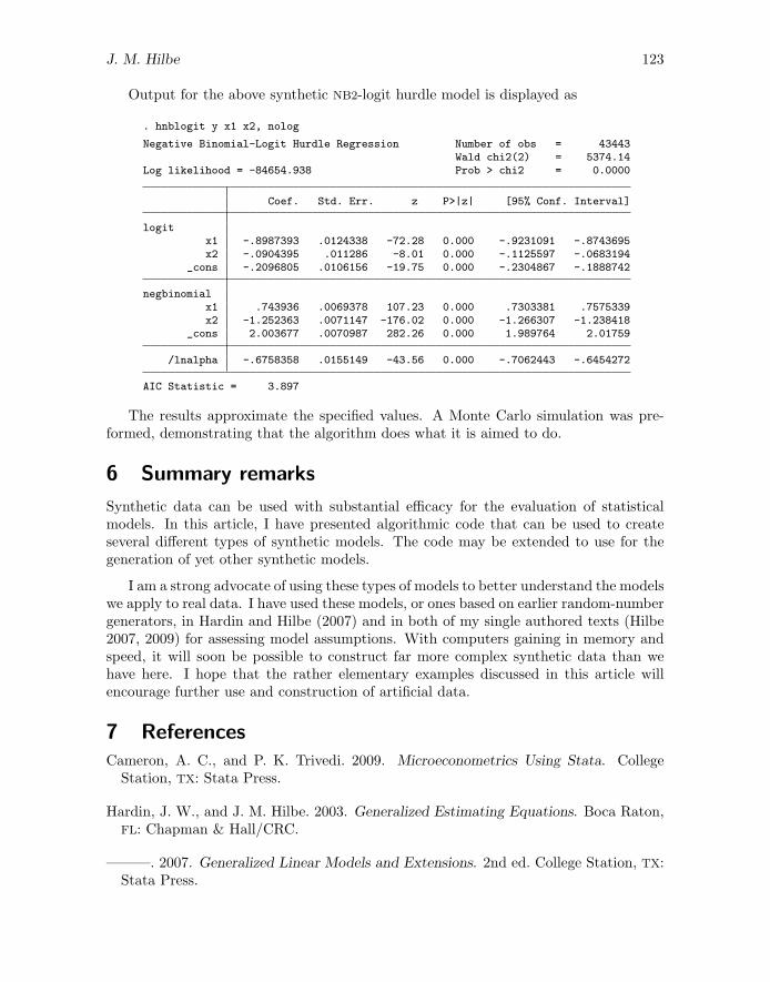
Output for the above synthetic NB2-logit hurdle model is displayed as

. hnblogit y x1 x2, nolog

Negative Binomial-Logit Hurdle Regression Number of obs = 43443Wald chi2(2) = 5374.14

Log likelihood = -84654.938 Prob > chi2 = 0.0000

Coef. Std. Err. z P>|z| [95% Conf. Interval]

logitx1 -.8987393 .0124338 -72.28 0.000 -.9231091 -.8743695x2 -.0904395 .011286 -8.01 0.000 -.1125597 -.0683194

_cons -.2096805 .0106156 -19.75 0.000 -.2304867 -.1888742

negbinomialx1 .743936 .0069378 107.23 0.000 .7303381 .7575339x2 -1.252363 .0071147 -176.02 0.000 -1.266307 -1.238418

_cons 2.003677 .0070987 282.26 0.000 1.989764 2.01759

/lnalpha -.6758358 .0155149 -43.56 0.000 -.7062443 -.6454272

AIC Statistic = 3.897

The results approximate the specified values. A Monte Carlo simulation was pre-formed, demonstrating that the algorithm does what it is aimed to do.

6 Summary remarks

Synthetic data can be used with substantial efficacy for the evaluation of statisticalmodels. In this article, I have presented algorithmic code that can be used to createseveral different types of synthetic models. The code may be extended to use for thegeneration of yet other synthetic models.

I am a strong advocate of using these types of models to better understand the modelswe apply to real data. I have used these models, or ones based on earlier random-numbergenerators, in Hardin and Hilbe (2007) and in both of my single authored texts (Hilbe2007, 2009) for assessing model assumptions. With computers gaining in memory andspeed, it will soon be possible to construct far more complex synthetic data than wehave here. I hope that the rather elementary examples discussed in this article willencourage further use and construction of artificial data.

7 References

Cameron, A. C., and P. K. Trivedi. 2009. Microeconometrics Using Stata. CollegeStation, TX: Stata Press.

Hardin, J. W., and J. M. Hilbe. 2003. Generalized Estimating Equations. Boca Raton,FL: Chapman & Hall/CRC.

———. 2007. Generalized Linear Models and Extensions. 2nd ed. College Station, TX:Stata Press.


Hilbe, J. M. 2007. Negative Binomial Regression. New York: Cambridge UniversityPress.

———. 2009. Logistic Regression Models. Boca Raton, FL: Chapman & Hall/CRC.

Hilbe, J. M., and W. Linde-Zwirble. 1995. sg44: Random number generators. StataTechnical Bulletin 28: 20–21. Reprinted in Stata Technical Bulletin Reprints, vol. 5,pp. 118–121. College Station, TX: Stata Press.

———. 1998. sg44.1: Correction to random number generators. Stata Technical Bulletin41: 23. Reprinted in Stata Technical Bulletin Reprints, vol. 7, p. 166. College Station,TX: Stata Press.

Long, J. S., and J. Freese. 2006. Regression Models for Categorical Dependent VariablesUsing Stata. 2nd ed. College Station, TX: Stata Press.

Winkelmann, R. 2008. Econometric Analysis of Count Data. 5th ed. Berlin: Springer.

About the author

Joseph M. Hilbe is an emeritus professor (University of Hawaii), an adjunct professor of statis-tics at Arizona State University, and Solar System Ambassador with the NASA/Jet PropulsionLaboratory, CalTech. He has authored several texts on statistical modeling, two of which areLogistic Regression Models (Chapman & Hall/CRC) and Negative Binomial Regression (Cam-bridge University Press). Hilbe is also chair of the ISI Astrostatistics Committee and Networkand was the first editor of the Stata Technical Bulletin (1991–1993).

Documents

Creating synthetic discrete-response regression modelsageconsearch.umn.edu/bitstream/152284/2/sjart_st0186.pdf · Creating synthetic discrete-response regression models ... negative