Credit Contagion Channels: Market Microstructure Evidence

Credit Contagion Channels: MarketMicrostructure Evidence from Lehman

Brothers’ Bankruptcy

Bidisha Chakrabarty and Gaiyan Zhang∗

Immediately after Lehman Brothers’ bankruptcy, many firms disclosed their financial exposure (orlack thereof) to Lehman. This offers a clean setting to test two credit contagion channels throughwhich a financial firm’s bankruptcy can affect other firms—“counterparty risk” and “informationtransmission” channels. Using market microstructure variables to measure the various dimensionsof contagion effects, we provide robust evidence supporting the significance of counterparty risk.Firms with exposure to Lehman suffered more severe negative effects—wider bid-ask spread, higherprice impact, greater information asymmetry, and greater selling pressure—than unexposed firms.We find mixed evidence regarding the information transmission hypothesis.

On September 15, 2008, Lehman Brothers Holdings, Inc. filed a petition in the US BankruptcyCourt for the Southern District of New York seeking relief under Chapter 11 of the US BankruptcyCode. With total debt close to $800 billion, Lehman was the largest US bankruptcy. Lehman’sshare lost over 90% of its value on the announcement date and the Dow Jones Industrial indexclosed over 500 points down from the previous day, one of the single largest one-day point dropssince September 11, 2001. Immediately in the aftermath of Lehman’s bankruptcy, over a hundredfirms disclosed their financial exposure (or lack thereof) to Lehman.

Lehman’s collapse, in conjunction with the disclosure of these firms’ financial exposure toLehman, provides us with a unique opportunity to test two competing theories of credit conta-gion: 1) counterparty risk and 2) information contagion arising from the bankruptcy of a largefinancial institution. The counterparty risk hypothesis predicts that firms with identifiable fi-nancial exposure to the failed firm should suffer adverse consequences because of fundamentalbusiness linkages (Davis and Lo, 2001). The information transmission hypothesis argues that thefailure of a firm causes investors to update their beliefs, leading to the financial distress of otherfirms, even if they have no direct business relationship with the failed firm (Giesecke, 2004;Collin-Dufresne, Goldstein, and Helwege, 2010).

To test these two theories of credit contagion, we manually collect information about the firms’financial exposure (or lack thereof) to Lehman.1 We classify firms into two groups: 1) exposedfirms that have some degree of exposure and 2) unexposed firms who declare (and we verify) that

We thank Jean Helwege, Philippe Jorion, Lawrence Kryzanowski, Bill Megginson, and seminar participants at theUniversity of Missouri, St. Louis and the 2010 Financial Management Association meetings for useful comments.

∗Bidisha Chakrabarty is an Associate Professor of Finance at Saint Louis University, St. Louis, MO. Gaiyan Zhang is anAssociate Professor of Finance at the University of Missouri, St. Louis, MO.

1 The majority of the firms that made voluntary declarations after Lehman’s collapse were financial firms. We use thissample of financial firms for our main analysis. In Section V, we do robustness tests by repeating our analysis with allfirms (both financial and nonfinancial) that made any declarations regarding their exposure or nonexposure to Lehman.

Financial Management • Summer 2012 • pages 319 - 343

320 Financial Management � Summer 2012

they have no exposure to Lehman. We then examine the relative changes in a number of liquidityvariables around the disclosure date for these two groups of firms. Relative change is calculatedas the difference between the disclosure day liquidity of the announcing firm and its controlperiod average, scaled by the control period average, to account for time series variations in thesevariables. Moreover, for each sample firm, we identify an industry and size matched firm withno financial exposure to Lehman (Industry and Size Matched [ISM] approach). This is used tocontrol for the impact of possible confounding events on the overall market on varying disclosuredates.2 Abnormal relative change in liquidity variables for a disclosing firm is calculated as thedifference in the relative change between each disclosing firm and its matching firm.

According to the information contagion hypothesis (Giesecke, 2004; Collin-Dufresne et al.,2010), the crisis creates a greater dispersion in beliefs amongst investors leading them to rapidlyupdate their beliefs in the postcrisis period. This should seem as abnormal trading behavior thatimpacts equity liquidity for all sample firms, with or without Lehman. Our full sample resultsindicate a dramatic increase in the bid-ask spread, the number of trades, trade size and volume,the adverse-selection component of the bid-ask spread, and the selling ratio on the announcementdate relative to the nonevent period reflecting greater uncertainty and abnormal trading behaviorarising from the announcement. The magnitude of abnormal relative change is smaller, butstatistically significant under the ISM approach. However, when we split the sample into exposedand unexposed firms, firms without exposure to Lehman exhibit abnormal increases in volume,but decreases in Kyle’s lambda under the ISM approach suggesting the price impact of trade issmaller, contrary to the information transmission hypothesis. There are no significant changes inthe other liquidity variables. Abnormal equity returns are positive, albeit insignificant. Thus, wefind mixed evidence for the information transmission hypothesis.

Consistent with the counterparty risk hypothesis, we find that firms with exposure to Lehmanexperience positive abnormal changes in the bid-ask spread, volume, Kyle’s Lambda, and theadverse selection component of spread suggesting that exposed firms suffer deterioration ofliquidity (e.g., higher transaction costs, greater price impact of trade, and decreased informationtransparency). In addition, there is significant negative order imbalance (evidenced by the highersell ratio) and negative returns for exposed firms. This provides direct evidence that investors aremore likely to sell stocks of exposed firms after their counterparty risk to Lehman is disclosedto the public. Moreover, when we compare the mean and median differences between the twogroups, the exposed firms experience significantly greater increase in the price impact of trades,information asymmetry, selling pressure, and lower equity returns than the unexposed firmssupporting the significance of the counterparty contagion effect.

In the financial services industry in particular, the size of institutions and the complexity oftheir business networks may lead to strong contagion effects by counterparty risk or informationtransmission channels. Identifying which contagion channel propagates the financial shock causedby a large bank failure has important policy implications. For example, Helwege (2010) arguesthat if information is the main contagion channel (i.e., banks with similar characteristics are likelyto be adversely affected), regulators should solve the common problems of these banks (e.g., if thecommon problem is their investment in mortgage-backed assets, the government should supportthe mortgage market) rather than supporting one failing bank. Alternatively, if counterparty riskis the major contagion channel, the government should bail out the bank that is likely to cause adomino effect within the financial system.

2 The matching sample approach is common in the microstructure literature as it is computationally prohibitive toconstruct microstructure variables for all firms in the market as a benchmark. We have also used the industry, size, andbook-to-market matching approach as robustness checks and the results are qualitatively similar.

Chakrabarty & Zhang � Credit Contagion Channels 321

Although it is importantto identify whether a shock propagates through information transmis-sion or counterparty contagion, prior studies have encountered two major problems in distin-guishing between these two channels. First, very few banks file for bankruptcy. In the categoryof “too big to fail,” Lehman is the only US case. In fact, in the days leading up to September15, 2008, as the market learned about the extent of Lehman’s financial problems, various res-cue packages were publicly being discussed.3 After the bailouts of (the much smaller financialfirms) Fannie Mae and Freddie Mac earlier in the week, the expectation was that some bailoutwould save Lehman from imminent collapse. In addition, it is difficult to identify (and thuscontrol for) counterparty relationships of a failed firm as such relationships are rarely disclosedto the public.4 Lehman’s bankruptcy, and the subsequent announcements by over 100 firmsdisclosing the extent of their exposure to Lehman, provides a unique context that allows us toexplicitly disentangle the sources of contagion effects from the collapse of a large financialinstitution.

Apart from this advantageous setting, an innovation of our study is that we use a number ofliquidity measures developed by the market microstructure literature to capture the high frequency,intraday impact of contagion effects on the liquidity of the affected firms’ stocks. These measuresinclude transaction costs, trading activity, the price impact of trade, information asymmetry, andselling pressure of the equity of disclosing firms. Although theoretical models make predictionsabout the specific dimensions of liquidity that may be affected because of contagion, previousempirical studies of credit contagion rely primarily on low frequency pricing data in the stock,bond, and credit default swap (CDS) markets.

Collin-Dufresne et al. (2010) use month-end bond prices and quotes to empirically test howcontagion effects of a major credit event spread to a corporate bond portfolio. In examining thecontagion effects of bankruptcies, Lang and Stulz (1992) measure abnormal equity returns (AR)of industry competitors after a bankruptcy filing. AR is calculated using the daily closing pricesfrom the Center for Research in Security Prices (CRSP) database. In studying the effects of afirm’s bankruptcy on the CDS spreads of its industry competitors, Jorion and Zhang (2007) useone CDS spread quote per day for a large sample of industry peer firms. In their subsequentstudy of counterparty risk, Jorion and Zhang (2009) examine CDS spread changes of creditorsof bankrupt firms.

In contrast to these studies, we examine the liquidity measures that can only be constructedfrom high frequency (tick-by-tick) data, and, as such, are able to test some of the predictions oftheoretical contagion models that cannot be inferred from daily/monthly observations. To citeone example, to examine sell pressure, we construct the sell ratio variable by identifying allbuyer-initiated and seller-initiated trades that are executed throughout the day. Thus, our studyprovides more accurate tests of the contagion theory from the market microstructure perspective.

Our paper contributes to the literature in three ways. First,this study adds to the growingliterature examining the impact of the bankruptcy of Lehman Brothers’ that, by all accounts, wasa major crisis event in recent financial history.5 Other studies that have examined counterparty

3 For example, two days before Lehman’s bankruptcy announcement, on September 13th, Timothy Geithner, then presidentof the Federal Reserve Bank of New York, called a meeting on the future of Lehman, which included the possibility ofan emergency liquidation of its assets (Anderson, Dash, Bajaj, and Andrews, 2008). Lehman also reported that it hadseparate talks with Bank of America and Barclays for a possible sale of the company (White and Anderson, 2008).4 Iyer and Peydro (2010) point out the two major problems in testing contagion because of interbank linkages are thedearth of large bank failures and the lack of detailed data on interbank linkages. They overcome these hurdles by using thesudden failure of a cooperative bank in India and a unique dataset that identifies exposure to study interbank contagion.5 Some recent studies discussing various dimensions of the crisis triggered by Lehman include Ivashina and Scharfstein(2010), Fernando, May, and Megginson (2011), Jorion and Zhang (2011) and Aragon and Strahan (2010).


contagion have examined smaller firms with limited interconnectedness. Of note is Jorion andZhang (2009) who focus on mostly industrial firms and a small group of financial institutionsthat went bankrupt, with their sample period ending before 2005.6 However, the counterpartyeffect could be more significant if the failed firm is a large financial firm and its counterpartyrelationships are complex. We find that the counterparty effect is much stronger than reported inJorion and Zhang (2009). In a recent Financial Crisis Inquiry Report, Federal Reserve ChairmanBernanke stated that 12 of the 13 largest banks in the US “were at risk of failure” at the depth of the2008 financial crisis.7 Therefore, the study of Lehman should shed light on possible contagioneffects arising from these large banks on the financial system had they also been allowed tofail.

Moreover, differing from Jorion and Zhang (2011), we provide a finer test of the credit contagionhypotheses using a number of market microstructure variables that allow us to directly examinethe trading behavior of market participants and the liquidity conditions of affected firms. Priorstudies have used microstructure variables to investigate various corporate events.8 We extendthis strand of the market microstructure literature to the study of credit contagion effects.

In addition, this is the first paper to test the information transmission hypothesis by explicitlycontrolling for a counterparty relationship. Prior studies that document market-wide or industry-wide contagion effects (Lang and Stulz, 1992; Collin-Dufresne et al., 2010) generally attributetheir findings to information contagion where investors update their beliefs about all other firmsin the market. Yet, what is identified as information contagion could be driven by firms withfundamental business linkages with the failed firm, leading to erroneous inferences because ofa failure to control for a counterparty relationship. The setting in our paper allows us to identifycounterparty relationships, thus disentangling these two channels. As previously mentioned,such a distinction carries important implications for government intervention policies during afinancial crisis.

The remainder of the paper is organized as follows. Section I reviews related literature anddevelops our hypotheses. Section II describes our sample and variables. Section III tests thecounterparty risk hypothesis and information transmission hypothesis. Section IV discusses someof the robustness check results, whereas Section V provides our conclusions.

I. Related Literature and Hypotheses Development

Credit contagion is the transmission of the financial distress or the downside shock of onecompany to other companies wherein, in some instances, it may push other companies intobankruptcy. This has been frequently observed during bankruptcy waves and during the recentfinancial crisis. Credit contagion is important in explaining observed clustering of default cor-relations (Das, Duffie, Kapadia, and Saita, 2007) and has implications for portfolio credit risk

6 The average total assets of firms in their sample are $1.9 billion, compared to $639 billion total assets for LehmanBrothers.7 Report Details Wall Street Crisis, By Carrick Mollenkamp, Aaron Lucchetti and Serena Ng, Wall Street Journal, Jan-uary 28, 2011. Source: http://online.wsj.com/article/SB10001424052748703399204576108461096848824.html?mod=dist_smartbrief.8 Examples of the market microstructure approach to study corporate events include takeover announcements on targetfirms (Jennings, 1994; Smith, White, Robinson, and Nason, 1997; King, 2009), stock splits (Easley, O’Hara, and Saar,2001), stock repurchases (Ahn, Cao, and Choe, 2001), seasoned equity offering (Butler, Grullon, and Weston, 2005;Kryzanowski, Lazrak, and Rakita, 2010), firm disclosures like earnings announcements (Krinsky and Lee, 1996), insidertrading (Inci, Lu, and Seyhun, 2010), and corporate misreporting and bank loan contracting (Graham, Li, and Qiu, 2008).


models (Duffie, Eckner, Horel, and Saita, 2009). We study two major credit contagion chan-nels that have been modeled in the literature, information contagion, and counterparty risk,which have different policy implications. As Helwege (2010) points out, if counterparty con-tagion is the major contagion channel, government bail-out of the failed firm is perhaps abetter policy response to save many other counterparty firms, whereas regulatory aid to onedistressed firm is of little use to boost confidence in the entire market if information is the majorchannel.

The information transmission hypothesis states that investors learn from defaults and updatetheir beliefs. For example, the failure of Enron led investors to reassess their views of thequality of the accounting information of other firms. In a theoretical framework, Collin-Dufresneet al. (2010) demonstrate that when investors have fragile beliefs, they will learn from realizeddefault events and rapidly update their beliefs in the postcrisis period, leading to contagionrisk premia. Giesecke (2004) develops a similar model based on the statistical modeling offrailty to explore learning-from-default interpretations. King and Wadhwani (1990) proposethat information asymmetry leads uninformed traders to update their beliefs about the terminalpayoffs of assets after idiosyncratic shocks to a single asset. Calvo (1999) and Yuan (2005)present informationally richer models that explore the consequences of insiders being financiallyconstrained and where uninformed investors cannot tell whether the observed selling activity isbecause of liquidity or real shocks. As such they may misread liquidity driven sales as signalingbad fundamentals.

Empirical investigations find support for information effects. For example, Lang and Stulz(1992) find that stock market reactions of their industry peer firms to nonfinancial firm bankrupt-cies are often negative. They posit that this is reflective of investors’ revaluations of assets in thatindustry. Collin-Dufresne et al. (2010) find strong reaction of the bond market index in responseto large credit shocks and attribute this to information contagion. However, these studies of theindustry or market-wide effects of contagion do not control for business relationships with thefailed firm. It is not clear whether and how much the companies in the same industry or inthe bond market index have exposures to the distressed firm. If the overall significant effect isdriven by firms that have economic linkages with the distressed firms, these results may reflectcounterparty risk instead of the information transmission mechanism.

Counterparty risk hypothesis states that the default of one firm causes financial distress forits creditors or other counterparties that have a direct linkage with the distressed firm. In theextreme case, this can push the counterparty toward default. Counterparty contagion should bestronger for financial institutions, given the intricate web of relationships within the bankingsystem. Counterparty risk has been analyzed in theoretical frameworks by Davis and Lo (2001),Giesecke and Weber (2004), and Boissay (2006).

One major problem in testing counterparty contagion is that it is usually difficult to identify thecounterparty of the distressed firm as such a relationship is rarely public knowledge. There are afew notable exceptions, however. Jorion and Zhang (2009) conduct a systematic test of counter-party contagion effects using bankruptcy court filing documents to identify the top 20 unsecuredcreditors, and find that counterparty risk is important in explaining contagion. However, theirbankruptcy sample covers mostly industrial firms, because the bankruptcy of US financial institu-tions has been fairly infrequent until recently. Furthermore, the average number of counterpartiesin their sample is only three public firms per bankruptcy. Iyer and Peydro (2011) use a suddenshock caused by a large bank failure in India and identify interbank exposures with a uniquedata source. They find that greater interbank exposure to the failed bank leads to large depositwithdrawals. Similar to the way they overcome the data hurdle, our study exploits the largelyunexpected bankruptcy of Lehman in conjunction with the disclosure of exposure to Lehman by


over one hundred companies. Our focus is different from theirs in that we attempt to disentanglethe information transmission from counterparty risk channels.

In gauging the negative consequences of contagion effects, prices of securities such as stocks,bonds, or CDS have been commonly used in prior studies. Although (price) return is one im-portant metric, there are various other dimensions of the effects of an adverse shock. First, thecrisis-induced information asymmetry should lead market makers to charge greater transactioncosts as measured by the quoted and effective bid-ask spread. Venkatesh and Chiang (1986)empirically document the increase in spread after information events. In addition, the arrivalof new information should trigger a greater dispersion in beliefs among investors, leading tomore intensive trading activities. Massa and Simonov (2005) find that uncertainty induced beliefdispersion increases both volume and volatility. Moreover, when trading becomes costly and eachtrade moves prices away from the last traded price (reduced ease of transaction), the price impactof trades should increase (Kyle, 1985). Furthermore, higher levels of information asymmetry inthe market should increase the adverse-selection component of the spread. Finally, the contagioneffect should manifest in increased liquidation orders by investors and lead to sell-side orderimbalance. Our market microstructure variables are suited to examine these various dimensionsof the contagion effects.

On the basis of our discussion above, we formulate the following two hypotheses:

H1: Information Transmission Hypothesis: The disclosure announcement creates a greater dis-persion in belief amongst investors, leading them to update their expectations and requirean uncertainty risk premium. Therefore, all sample firms, with or without exposure toLehman, should have greater bid-ask spreads, increased trading activities, higher price im-pacts of trade, greater levels of information asymmetry, and greater sell order imbalanceson the disclosure day compared to the control period.

H2: Counterparty Risk Hypothesis: Firms with exposure to Lehman should suffer more severeadverse consequences than unexposed firms as a result of direct credit losses or potentiallosses because of lost business relationships. Therefore, the exposed firms should havehigher bid-ask spreads, more trading activities, greater price impact of trade, greater levelsof information asymmetry, and more selling pressure than the unexposed firms.

Our study adds to the growing list of papers investigating a variety of issues in the contextof Lehman Brothers’ bankruptcy. For example, Ivashina and Scharfstein (2010) examine banklending behavior during the crisis and find that after the failure of Lehman Brothers, there wasa run by short-term bank creditors, making it difficult for banks to roll over their short-termdebt. They also demonstrate that banks with greater cosyndication with Lehman suffered moreliquidity stress, indicating that Lehman’s failure put more of the funding burden on other membersof the syndicate and increased the likelihood that more firms would draw on their credit lines.Fernando, May, and Megginson (2011) investigate the value of investment banking relationshipsby exploring the impact of Lehman’s bankruptcy on clients of its underwriting business. They findthat firms that employed Lehman for equity offerings suffered during Lehman’s bankruptcy. Theirsample excludes firms with exposure to Lehman, though. Aragon and Strahan (2010) examinethe role of hedge funds as liquidity providers using evidence from the Lehman bankruptcy. Theyfind that stocks traded by the Lehman-connected hedge funds experienced greater declines inliquidity than other stocks. More broadly, our study also relates to the assessment of contagioneffects during the recent subprime crisis, as examined in the context of hedge funds by Dudleyand Nimalendran (2011) and the study of the sector level contagion effect by Phylaktis and Xia(2009).


II. Sample and Variables

A. Sample

Our data come from several sources. Over 100 firms voluntarily disclosed their exposure toLehman after its bankruptcy and provided detailed information on the type and amount of thisexposure. Several of them stated that their business relationships with Lehman are not expectedto have an adverse material effect on their financial condition or liquidity. This is most likely toreassure investors and reduce speculation arising from information uncertainty or information-based contagion because of imperfect information. Some other firms also made public statementsat that time that they did not have any financial exposure to Lehman. We hand-collect informationon all such firms that disclose their exposure (or lack thereof) to Lehman in the two weeks afterLehman’s bankruptcy from various news sources and cross-check using the Lexis–Nexis newsdatabase and Securities and Exchange Commission (SEC) filings. We include those firms thatdeclared they had exposure into the exposed sample and the ones that indicated they had (and weverified) no exposure in the unexposed group.

In addition, we gather information for firms with exposure from the bankruptcy filing docu-ments of Lehman Brothers that disclose the top 30 unsecured claimholders on bankruptcy dayincluding creditor names, credit types, and credit amounts extended to the bankrupt firm. Ofthese, four firms have returns data from CRSP and are included in our sample.9

We use the Lexis–Nexis database to search for news items for our initial sample of voluntarilydisclosing firms and exclude several firms that experienced other significant corporate eventseither in our testing (event) days or in the control period (August 2008). These firms includeFannie Mae and Freddie Mac that were nationalized on September 8, 2008, Bank of America andMerrill Lynch that reached an acquisition plan on September 15, 2008, Barclays that acquired(postbankruptcy) Lehman Brothers on September 16, Goldman Sachs and Morgan Stanley thatwere converted into “bank holding companies” on September 22, Washington Mutual that wasseized by the Federal Deposit Insurance Corporation (FDIC) on September 25, and Wachoviathat was in distress and acquired by Wells Fargo in early October.10

Our purpose is to examine abnormal changes in liquidity for firms that disclose information onexposure to Lehman around the disclosure date relative to the nonevent control period.11 Insteadof examining the changes in the levels of liquidity variables around a firm’s disclosure date, weconstruct the relative changes (in percentage) of liquidity variables to control for variations inliquidity variable levels across sample firms. Disclosure date is the date on which each samplefirm announces publicly, for the first time, its exposure (or lack thereof) to Lehman. Disclosuredates range from September 15, 2008 to September 24, 2008. The control period, against whichwe compare the event period changes, is August 2008. We require these firms to have data onthe NYSE’s Trade and Quote (TAQ) database, stock price information in the CRSP database,

9 For these firms, the disclosure date is the bankruptcy filing date.10 Although the Wachovia takeover date falls outside our testing period, we eliminate this firm as the possibility of itstakeover was already in the news by mid-September.11 Instead of Lehman’s bankruptcy date, we use the disclosure date of each firm as its event date because the informationon exposure to Lehman was not known to the public until the disclosure was made after Lehman’s bankruptcy date. Thus,we cannot capture contagion because of the counterparty relationship on the bankruptcy date. Further in the manuscript,we construct a variable, Sellratio, which is a measure of the relative sell pressure in the market for firms disclosing theirfinancial exposures to Lehman. We find that in the days before the disclosure announcement was made, this Sellratiovariable is almost always close to 50% indicating that traders did not rush to sell off stocks in these firms, corroboratingthe fact that the exposure announcements were largely unanticipated by the market.


and company information in the Compustat database. The final sample includes 86 firms, 60 ofwhich are financial institutions (standard industrial classification [SIC] Code 6XXX). For ourmain tests, we focus on this sample of 60 financial firms, of which 47 have exposure to Lehman.In later robustness tests, we replicate all of our results with the full sample of 86 firms, of which56 have exposure to Lehman.

To control for volatile market conditions on different disclosure dates after Lehman’sbankruptcy, we construct an industry-size matched sample of firms against which we com-pare our sample firms. To construct the matching sample, we begin with all firms that have thesame two-digit SIC code as the disclosing firm. Then, we identify the firm with the closest marketcapitalization as the disclosing firm as its matching firm. Notably, after obtaining each match,we verify from each company’s 10-K and 10-Q disclosures that they make no mention of anyfinancial relationship with Lehman Brothers.

We calculate relative (percentage) changes in liquidity variables for this matched sample, andthen measure the pure impact of exposure on the disclosing firms as the relative change inliquidity variables for the sample firms minus the corresponding relative changes of the matchedfirms.12 We expect our methodology to ensure that the main driver of the difference in equityreturns and microstructure variables between the disclosing firms and their matched counterpartsis exposure to Lehman, rather than market conditions, industry, or size differences. Our approachshould provide clean estimates of the effect of exposure to Lehman on the sample firms.

We measure a firm’s exposure as credit claims, including direct exposure to Lehman’s debt(i.e., commercial paper, notes, bonds, and bank loans issued by Lehman). Reported exposures,however, also include positions in preferred stock and common stock. Firms also report theirexposure arising from derivatives contracts. This includes CDS protection sold on Lehman, aswell as derivatives positions entered into with Lehman that have positive value and, as such, areexposed to counterparty risk.

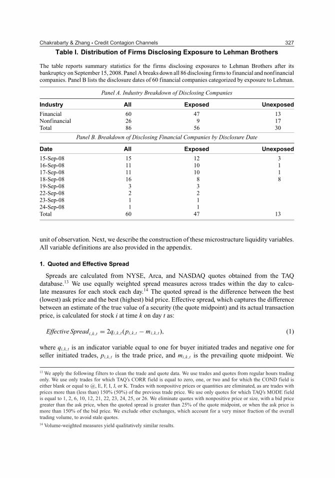
In Panel A of Table I, we provide a breakdown of all the declaring firms into financialcompanies and nonfinancial companies. Among the 86 firms in our sample, 60 are in the finance,insurance, and real estate sector with 47 exposed firms and 13 unexposed firms. Panel B limitsthe sample to financial firms and reports the dates on which these firms voluntarily disclose theirexposure to Lehman Brothers. 15 of the 60 firms announced their exposure (zero or positive) onthe very day of Lehman’s bankruptcy. Within the next three days, 53 of the 60 (over 88% of thesample) had made the extent of their exposure known.

B. Variables

We use the number of trades, average trade size, and trade volume aggregated at the dailyfrequency to measure the trading activities of disclosing firms. In addition, we use quoted andeffective spread, Kyle’s Lambda, adverse selection cost, and sell ratio to measure the liquidityconditions and information asymmetry of the disclosing firms. All the variables are collectedintraday and averaged for each stock each day. We then average each variable for each samplestock over all sample days and report the average across stocks, in effect treating each stock as a

12 Such a matched sample approach is common to microstructure studies because it is computationally prohibitive toconstruct microstructure variables for all firms in the market as a benchmark (Bessembinder, 1999, 2003; Chung,Van Ness, and Van Ness, 2001). Davies and Kim (2009) explain the advantages of the matching approach in marketmicrostructure research. Following Eberhart, Altman, and Aggarwal (1999), we adopt the industry and size matchingapproach, which has been commonly used in the credit risk literature to control for industry risk. We have also usedanother matching approach (i.e., industry, size, and book-to-market [ISM] approach) as in Eberhart et al. (1999) to identifymatching firms. The results are qualitatively similar.


Table I. Distribution of Firms Disclosing Exposure to Lehman Brothers

The table reports summary statistics for the firms disclosing exposures to Lehman Brothers after itsbankruptcy on September 15, 2008. Panel A breaks down all 86 disclosing firms to financial and nonfinancialcompanies. Panel B lists the disclosure dates of 60 financial companies categorized by exposure to Lehman.

Panel A. Industry Breakdown of Disclosing Companies

Industry All Exposed Unexposed

Financial 60 47 13Nonfinancial 26 9 17Total 86 56 30

Panel B. Breakdown of Disclosing Financial Companies by Disclosure Date

Date All Exposed Unexposed

15-Sep-08 15 12 316-Sep-08 11 10 117-Sep-08 11 10 118-Sep-08 16 8 819-Sep-08 3 322-Sep-08 2 223-Sep-08 1 124-Sep-08 1 1Total 60 47 13

unit of observation. Next, we describe the construction of these microstructure liquidity variables.All variable definitions are also provided in the appendix.

1. Quoted and Effective Spread

Spreads are calculated from NYSE, Arca, and NASDAQ quotes obtained from the TAQdatabase.13 We use equally weighted spread measures across trades within the day to calcu-late measures for each stock each day.14 The quoted spread is the difference between the best(lowest) ask price and the best (highest) bid price. Effective spread, which captures the differencebetween an estimate of the true value of a security (the quote midpoint) and its actual transactionprice, is calculated for stock i at time k on day t as:

Effective Spreadi,k,t = 2qi,k,t (pi,k,t − mi,k,t ), (1)

where qi,k,t is an indicator variable equal to one for buyer initiated trades and negative one forseller initiated trades, pi,k,t is the trade price, and mi,k,t is the prevailing quote midpoint. We

13 We apply the following filters to clean the trade and quote data. We use trades and quotes from regular hours tradingonly. We use only trades for which TAQ’s CORR field is equal to zero, one, or two and for which the COND field iseither blank or equal to @, E, F, I, J, or K. Trades with nonpositive prices or quantities are eliminated, as are trades withprices more than (less than) 150% (50%) of the previous trade price. We use only quotes for which TAQ’s MODE fieldis equal to 1, 2, 6, 10, 12, 21, 22, 23, 24, 25, or 26. We eliminate quotes with nonpositive price or size, with a bid pricegreater than the ask price, when the quoted spread is greater than 25% of the quote midpoint, or when the ask price ismore than 150% of the bid price. We exclude other exchanges, which account for a very minor fraction of the overalltrading volume, to avoid stale quotes.14 Volume-weighted measures yield qualitatively similar results.


follow the trade signing approach of Lee and Ready (1991) where a trade is classified as buyerinitiated if the trade price is above the quote midpoint and as seller initiated if the trade price isbelow the quote midpoint. Trades occurring at the midpoint between the best bid and the bestoffer are classified as seller initiated (buyer initiated) if the trade price is lower (higher) than theprice of the previous trade. We use contemporaneous quotes to sign trades because Chakrabarty,Moulton, and Shkilko (2011) find that daily level studies need not lag quotes when using theLee–Ready (1991) algorithm. Greater quoted and effective spreads indicate higher transactioncosts and lower stock liquidity.

2. (Kyle’s) Lambda

Microstructure models predict that trading costs increase with the degree of information asym-metry in the market (Glosten and Milgrom, 1985; Kyle, 1985). The amount that a risk-neutral andcompetitive market maker charges to protect them against adverse selection increases with thedegree of information asymmetry and decreases with the amount of noise trading. Kyle (1985)models this cost as the price impact of trade, �P = λV , where V is the number of shares tradedand λ, commonly known as Kyle’s Lambda, is the price impact per unit of trade. Kyle (1985)finds that λ is proportional to the standard deviation, σ , of the distribution of possible fair valuesof the security, and inversely proportional to the standard deviation of the distribution of tradesby noise traders, σ u: λ = 2 σ / σ u.

3. Glosten and Harris Adverse Selection Component of Spread

Spread decomposition models in the market microstructure literature split the bid-ask spreadinto three components: 1) inventory holding costs (price risk and opportunity cost of holding asuboptimal portfolio of securities), 2) order processing costs (costs of arranging trades, recording,and clearing a transaction), and 3) adverse selection costs (costs that arise if investors tradeon the basis of superior information). The adverse selection cost represents the compensationthat market liquidity suppliers need to be willing to trade with informed investors. Oliver andVerrecchia (1994)argue that some well informed investors possess a better ability to analyzepublicly available data and convert it into private information. As the market makers are unableto differentiate between the processors and the uninformed investors, they protect themselves bycharging a higher spread. Therefore, uninformed traders lose to informed traders implicitly byhaving to pay wider spreads induced by this adverse selection problem. The level of informationasymmetry is captured in the adverse-selection component of the bid-ask spread. A higher level ofthe adverse selection component of the bid-ask spread indicates greater information asymmetryand more informed trading.

Trade indicator models compute spread components by regressing price changes on a tradeindicator variable. One such model is the Glosten and Harris (1988) model which assumes thatthe different spread components have a linear relationship with trade size. Their model producesthe best estimates when order processing costs are fixed and the adverse selection componentcost increases with trade size.15

15 In the Glosten-Harris (1988) model that we use to estimate the adverse selection component of spread, the linearregression equation can be written as: �Pt = c0�Qt + c1�QtVt + z0Qt + z1QtVt + εt , where Pt is the trade price at timet, Qt is a trade indicator equal to +1 (–1) if the trade is buyer (seller) initiated, Vt is the number of shares traded at timet, and εt is the public information arrival rate which also represents the error term. In this model, the adverse selectioncomponent is 2(z0 + z1Vt). An alternative to the adverse selection component of spread would be the PIN, probability ofinformed trading, estimate. We choose to estimate the former as PIN is generally calculated over longer periods of timeand, by our study design, the abnormal measures we calculate are for very short (daily) frequencies.


4. Sell Ratio

Intraday data allow us to use the Lee–Ready (1991) algorithm to classify trades into buyerand seller initiated. We use this algorithm to examine whether there is selling pressure once thesample firms disclose their degree of exposure to Lehman. To do this, we construct two measures:1) Sellratio and 2) Lagged Sellratio. Sellratio is the number of seller initiated trades divided bythe total trades, whereas Lagged Sellratio is the Sellratio measure computed for the previousday. This measure has also been used by Jakob and Ma (2003) to measure order imbalance onexdividend days and is better suited than the normal scaled order imbalance measure.16

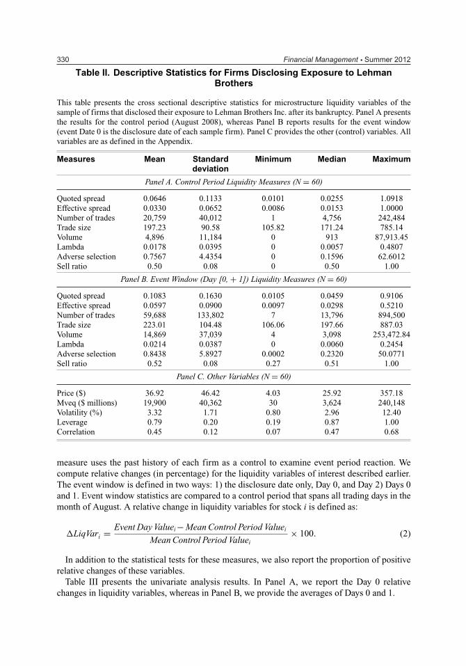
Table II presents the descriptive characteristics of the sample. Panel A provides the control pe-riod measures for the liquidity variables, whereas Panel B reports the event window (Days [0, +1]relative to each firm’s exposure disclosure date) measures. Both quoted and effective spreads in-crease upon exposure announcements. Mean quoted spread increases from 6.5 to 10.8 centsand mean effective spread increases from 3.3 to 6 cents. Quoted spread is higher than effectivespread, indicating that some trades happen within (not at) the best quotes. Despite this increasedtransaction cost (spread increase), there is a huge volume surge upon disclosure. The averagenumber of trades per day increases from 20,759 to 59,688 along with increased trade size (from197 to 223 shares per trade). Adverse selection increases from 0.75 to 0.84, reflecting increasedinformation asymmetry. Increased volume counterbalances increased spreads, such that the priceimpact variable, Kyle’s lambda, indicates a modest change between the control period (0.018)and the event window (0.021).

The mean Sellratio in the control period (Panel A) is 50%, indicating that buy and sell pressureare generally equally balanced daily in the month of August (before the bankruptcy announce-ment). This confirms that the bankruptcy announcement was indeed unexpected, and there wasno run-up to order flow before the exposure announcement. However, in the event window, wefind an increase of the sell pressure to 52% over days (0, +1).

Panel C presents the firm level characteristics of the sample. The sample is comprised of mostlylarge capitalization firms. The average market value of equity for the sample firms precedingthe Lehman Brothers’ bankruptcy (September 12, 2008) is just under $20 billion and the averagestock price is about $37. Volatility, the average daily stock return volatility for the disclosing firmover the preceding year is 3.32%, ranging from 0.80% to 12.40%. Leverage, the average leverageratio of the disclosing firm over four quarters during the preceding year, is 0.79. The leverageratio is defined as the ratio of the book value of debt over the market value of assets, taken asthe market value of equity plus the book value of debt. As expected, because the sample firms allbelong to the financial sector, they have a high degree of correlation (0.45) between their equityreturns and Lehman’s equity returns over the preceding year.

III. Testing Information Transmission and Counterparty RiskHypotheses

A. Univariate Analysis of Relative Changes and Abnormal Changes in LiquidityMeasures

To examine the market reaction to the sample firms’ disclosure regarding their exposure toLehman, we use the event study methodology described in Corwin and Lipson (2000). This

16 Raw order imbalance is measured as the difference between the number of buyer initiated orders and the number ofseller initiated orders. To scale this, we cannot use the average control period imbalance as the denominator because acontrol period, when it is appropriately chosen and is free of unusual events, has extremely low (zero) order imbalance.When the denominator is close to zero, the abnormal percentage changes can tend to infinity.


Table II. Descriptive Statistics for Firms Disclosing Exposure to LehmanBrothers

This table presents the cross sectional descriptive statistics for microstructure liquidity variables of thesample of firms that disclosed their exposure to Lehman Brothers Inc. after its bankruptcy. Panel A presentsthe results for the control period (August 2008), whereas Panel B reports results for the event window(event Date 0 is the disclosure date of each sample firm). Panel C provides the other (control) variables. Allvariables are as defined in the Appendix.

Measures Mean Standard Minimum Median Maximumdeviation

Panel A. Control Period Liquidity Measures (N = 60)

Quoted spread 0.0646 0.1133 0.0101 0.0255 1.0918Effective spread 0.0330 0.0652 0.0086 0.0153 1.0000Number of trades 20,759 40,012 1 4,756 242,484Trade size 197.23 90.58 105.82 171.24 785.14Volume 4,896 11,184 0 913 87,913.45Lambda 0.0178 0.0395 0 0.0057 0.4807Adverse selection 0.7567 4.4354 0 0.1596 62.6012Sell ratio 0.50 0.08 0 0.50 1.00

Panel B. Event Window (Day [0, + 1]) Liquidity Measures (N = 60)

Quoted spread 0.1083 0.1630 0.0105 0.0459 0.9106Effective spread 0.0597 0.0900 0.0097 0.0298 0.5210Number of trades 59,688 133,802 7 13,796 894,500Trade size 223.01 104.48 106.06 197.66 887.03Volume 14,869 37,039 4 3,098 253,472.84Lambda 0.0214 0.0387 0 0.0060 0.2454Adverse selection 0.8438 5.8927 0.0002 0.2320 50.0771Sell ratio 0.52 0.08 0.27 0.51 1.00

Panel C. Other Variables (N = 60)

Price ($) 36.92 46.42 4.03 25.92 357.18Mveq ($ millions) 19,900 40,362 30 3,624 240,148Volatility (%) 3.32 1.71 0.80 2.96 12.40Leverage 0.79 0.20 0.19 0.87 1.00Correlation 0.45 0.12 0.07 0.47 0.68

measure uses the past history of each firm as a control to examine event period reaction. Wecompute relative changes (in percentage) for the liquidity variables of interest described earlier.The event window is defined in two ways: 1) the disclosure date only, Day 0, and Day 2) Days 0and 1. Event window statistics are compared to a control period that spans all trading days in themonth of August. A relative change in liquidity variables for stock i is defined as:

�LiqVari = Event Day Valuei− Mean Control Period Valuei

Mean Control Period Valuei× 100. (2)

In addition to the statistical tests for these measures, we also report the proportion of positiverelative changes of these variables.

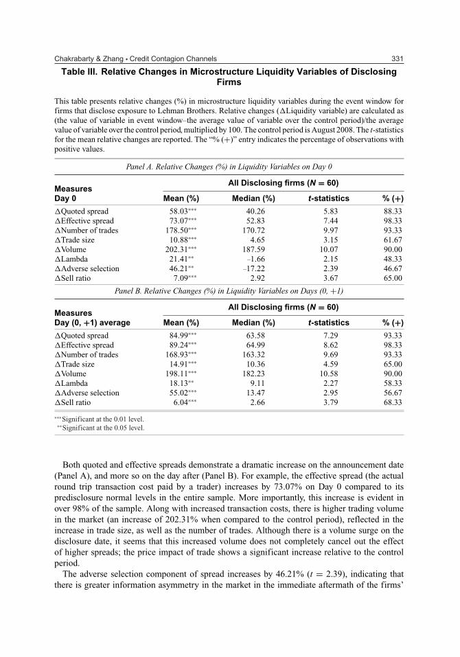
Table III presents the univariate analysis results. In Panel A, we report the Day 0 relativechanges in liquidity variables, whereas in Panel B, we provide the averages of Days 0 and 1.


Table III. Relative Changes in Microstructure Liquidity Variables of DisclosingFirms

This table presents relative changes (%) in microstructure liquidity variables during the event window forfirms that disclose exposure to Lehman Brothers. Relative changes (�Liquidity variable) are calculated as(the value of variable in event window–the average value of variable over the control period)/the averagevalue of variable over the control period, multiplied by 100. The control period is August 2008. The t-statisticsfor the mean relative changes are reported. The “% (+)” entry indicates the percentage of observations withpositive values.

Panel A. Relative Changes (%) in Liquidity Variables on Day 0

All Disclosing firms (N = 60)MeasuresDay 0 Mean (%) Median (%) t-statistics % (+)

�Quoted spread 58.03∗∗∗ 40.26 5.83 88.33�Effective spread 73.07∗∗∗ 52.83 7.44 98.33�Number of trades 178.50∗∗∗ 170.72 9.97 93.33�Trade size 10.88∗∗∗ 4.65 3.15 61.67�Volume 202.31∗∗∗ 187.59 10.07 90.00�Lambda 21.41∗∗ –1.66 2.15 48.33�Adverse selection 46.21∗∗ –17.22 2.39 46.67�Sell ratio 7.09∗∗∗ 2.92 3.67 65.00

Panel B. Relative Changes (%) in Liquidity Variables on Days (0, +1)

All Disclosing firms (N = 60)MeasuresDay (0, +1) average Mean (%) Median (%) t-statistics % (+)

�Quoted spread 84.99∗∗∗ 63.58 7.29 93.33�Effective spread 89.24∗∗∗ 64.99 8.62 98.33�Number of trades 168.93∗∗∗ 163.32 9.69 93.33�Trade size 14.91∗∗∗ 10.36 4.59 65.00�Volume 198.11∗∗∗ 182.23 10.58 90.00�Lambda 18.13∗∗ 9.11 2.27 58.33�Adverse selection 55.02∗∗∗ 13.47 2.95 56.67�Sell ratio 6.04∗∗∗ 2.66 3.79 68.33

∗∗∗Significant at the 0.01 level.∗∗Significant at the 0.05 level.

Both quoted and effective spreads demonstrate a dramatic increase on the announcement date(Panel A), and more so on the day after (Panel B). For example, the effective spread (the actualround trip transaction cost paid by a trader) increases by 73.07% on Day 0 compared to itspredisclosure normal levels in the entire sample. More importantly, this increase is evident inover 98% of the sample. Along with increased transaction costs, there is higher trading volumein the market (an increase of 202.31% when compared to the control period), reflected in theincrease in trade size, as well as the number of trades. Although there is a volume surge on thedisclosure date, it seems that this increased volume does not completely cancel out the effectof higher spreads; the price impact of trade shows a significant increase relative to the controlperiod.

The adverse selection component of spread increases by 46.21% (t = 2.39), indicating thatthere is greater information asymmetry in the market in the immediate aftermath of the firms’


announcements. It is interesting to note that the disclosure of exposure (if any) to Lehman alreadyreflects the fact that the disclosing companies anticipated they might face some repercussionsfrom the bankruptcy announcement. These public disclosures were a way of reducing informationasymmetry to preempt precipitate reaction from traders. The relative change in the sell ratio is7.09% (t = 3.67) indicating greater sell pressure after the exposure announcements.

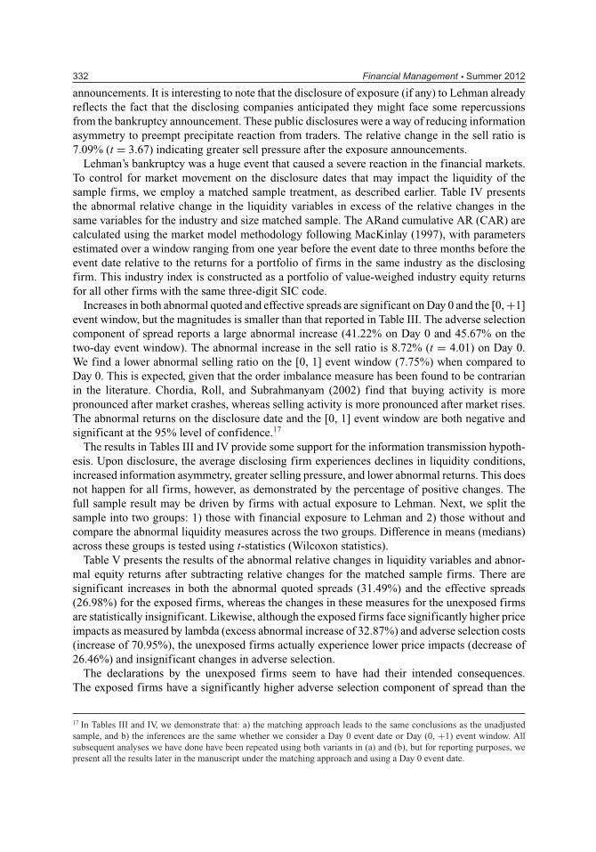
Lehman’s bankruptcy was a huge event that caused a severe reaction in the financial markets.To control for market movement on the disclosure dates that may impact the liquidity of thesample firms, we employ a matched sample treatment, as described earlier. Table IV presentsthe abnormal relative change in the liquidity variables in excess of the relative changes in thesame variables for the industry and size matched sample. The ARand cumulative AR (CAR) arecalculated using the market model methodology following MacKinlay (1997), with parametersestimated over a window ranging from one year before the event date to three months before theevent date relative to the returns for a portfolio of firms in the same industry as the disclosingfirm. This industry index is constructed as a portfolio of value-weighed industry equity returnsfor all other firms with the same three-digit SIC code.

Increases in both abnormal quoted and effective spreads are significant on Day 0 and the [0, +1]event window, but the magnitudes is smaller than that reported in Table III. The adverse selectioncomponent of spread reports a large abnormal increase (41.22% on Day 0 and 45.67% on thetwo-day event window). The abnormal increase in the sell ratio is 8.72% (t = 4.01) on Day 0.We find a lower abnormal selling ratio on the [0, 1] event window (7.75%) when compared toDay 0. This is expected, given that the order imbalance measure has been found to be contrarianin the literature. Chordia, Roll, and Subrahmanyam (2002) find that buying activity is morepronounced after market crashes, whereas selling activity is more pronounced after market rises.The abnormal returns on the disclosure date and the [0, 1] event window are both negative andsignificant at the 95% level of confidence.17

The results in Tables III and IV provide some support for the information transmission hypoth-esis. Upon disclosure, the average disclosing firm experiences declines in liquidity conditions,increased information asymmetry, greater selling pressure, and lower abnormal returns. This doesnot happen for all firms, however, as demonstrated by the percentage of positive changes. Thefull sample result may be driven by firms with actual exposure to Lehman. Next, we split thesample into two groups: 1) those with financial exposure to Lehman and 2) those without andcompare the abnormal liquidity measures across the two groups. Difference in means (medians)across these groups is tested using t-statistics (Wilcoxon statistics).

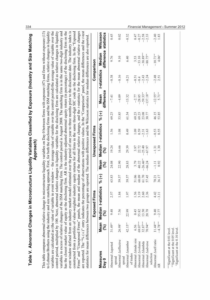
Table V presents the results of the abnormal relative changes in liquidity variables and abnor-mal equity returns after subtracting relative changes for the matched sample firms. There aresignificant increases in both the abnormal quoted spreads (31.49%) and the effective spreads(26.98%) for the exposed firms, whereas the changes in these measures for the unexposed firmsare statistically insignificant. Likewise, although the exposed firms face significantly higher priceimpacts as measured by lambda (excess abnormal increase of 32.87%) and adverse selection costs(increase of 70.95%), the unexposed firms actually experience lower price impacts (decrease of26.46%) and insignificant changes in adverse selection.

The declarations by the unexposed firms seem to have had their intended consequences.The exposed firms have a significantly higher adverse selection component of spread than the

17 In Tables III and IV, we demonstrate that: a) the matching approach leads to the same conclusions as the unadjustedsample, and b) the inferences are the same whether we consider a Day 0 event date or Day (0, +1) event window. Allsubsequent analyses we have done have been repeated using both variants in (a) and (b), but for reporting purposes, wepresent all the results later in the manuscript under the matching approach and using a Day 0 event date.


Table IV. Abnormal Relative Changes in Microstructure Liquidity Variables ofDisclosing Firms (Industry and Size Matching Approach)

This table presents abnormal relative changes in microstructure liquidity variables during the event windowfor firms that disclose exposure to Lehman Brothers using the industry and size matching approach. Weproceed in two steps. First, for both the disclosing firms and the ISM matching firms, relative changes inliquidity variables are calculated as (the value of variable in event window − the average value of variableover the control period)/the average value of variable over the control period, multiplied by 100. Next,abnormal relative changes in liquidity variables for the disclosing firm are calculated as relative changesin liquidity variables in excess of relative changes of the ISM matching firm. The matching firm is in thesame two-digit industry and has the closest market value of equity as the disclosing firm. AR (CAR) isthe industry-adjusted abnormal (cumulative abnormal) return (in percentage) of the disclosing firm on theevent window defined from an industry market model estimated over the period of one year to three monthsbefore the disclosure date. The industry index is constructed from a portfolio of value-weighted industryequity returns for all firms in the same three-digit SIC code as the disclosing firm. The t-statistics for themean abnormal relative changes are reported. The “% (+)” entry indicates the fraction of observations withpositive values.

Panel A. Abnormal Changes (%) in Liquidity Variables on Day 0

All disclosing firms (N = 60)MeasuresDay 0 Mean (%) Median (%) t-statistics % (+)

Abnormal �quoted spread 29.88∗∗∗ 16.29 2.96 65.00Abnormal �effective spread 26.09∗∗ 10.96 2.12 58.33Abnormal �number of trades 39.26∗ 26.19 1.88 60.00Abnormal �trade size 5.95∗ 3.41 1.77 55.00Abnormal �volume 62.82∗∗∗ 54.05 2.83 68.33Abnormal �lambda 20.01∗ –0.50 1.91 51.67Abnormal �adverse selection 41.22 2.16 1.58 51.67Abnormal �sell ratio 8.72∗∗∗ 3.65 4.01 65.00AR −3.54∗∗∗ −1.56 −2.75 40.00

Panel B. Abnormal Changes (%) in Liquidity Variables on Day (0, +1)

All disclosing firms (N = 60)MeasuresDay (0, +1) average Mean (%) Median (%) t-statistics % (+)

Abnormal �quoted spread 54.09∗∗∗ 32.11 4.55 68.33Abnormal �effective spread 37.81∗∗∗ 21.92 3.03 60.00Abnormal �number of trades 29.69 24.84 1.24 58.33Abnormal �trade size 9.97∗∗∗ 5.43 2.99 61.67Abnormal �volume 58.62∗∗ 34.94 2.38 61.67Abnormal �lambda 20.04∗∗ 1.15 2.23 53.33Abnormal �adverse selection 45.67∗ 25.21 1.93 60.00Abnormal �sell ratio 7.74∗∗∗ 3.04 4.19 66.67CAR −3.42∗ −2.97 −1.82 40.00

∗∗∗Significant at the 0.01 level.∗∗Significant at the 0.05 level.∗Significant at the 0.10 level.

334 Financial Management � Summer 2012T

able

V.

Ab

no

rmal

Ch

ang

esin

Mic

rost

ruct

ure

Liq

uid

ity

Var

iab

les

Cla

ssifi

edb

yE

xpo

sure

(In

du

stry

and

Siz

eM

atch

ing

Ap

pro

ach

)

Thi

sta

ble

com

pare

sab

norm

alre

lativ

ech

ange

inm

icro

stru

ctur

eli

quid

ity

vari

able

son

Day

0be

twee

nfi

rms

wit

hex

posu

re(4

7)an

dfi

rms

wit

hout

expo

sure

(13)

toL

ehm

anB

roth

ers

usin

gth

ein

dust

ryan

dsi

zem

atch

ing

appr

oach

.Fir

st,f

orbo

thth

edi

sclo

sing

firm

san

dth

eIS

Mm

atch

ing

firm

s,re

lativ

ech

ange

sin

liqu

idit

yva

riab

les

are

calc

ulat

edas

(the

valu

eof

vari

able

inev

entw

indo

w−

the

aver

age

valu

eof

vari

able

over

the

cont

rolp

erio

d)/t

heav

erag

eva

lue

ofva

riab

leov

erth

eco

ntro

lpe

riod

,mul

tipl

ied

by10

0.N

ext,

abno

rmal

rela

tive

chan

ges

inli

quid

ity

vari

able

sfo

rth

edi

sclo

sing

firm

are

calc

ulat

edas

rela

tive

chan

ges

inli

quid

ity

vari

able

sin

exce

ssof

rela

tive

chan

ges

ofth

eIS

Mm

atch

ing

firm

.The

cont

rolp

erio

dis

Aug

ust2

008.

The

mat

chin

gfi

rmis

inth

esa

me

two-

digi

tind

ustr

yan

dha

sth

ecl

oses

tm

arke

tva

lue

ofeq

uity

asth

edi

sclo

sing

firm

.AR

isth

ein

dust

ry-a

djus

ted

abno

rmal

equi

tyre

turn

(in

perc

enta

ge)

ofth

edi

sclo

sing

firm

onth

eev

ent

win

dow

defi

ned

from

anin

dust

rym

arke

tmod

eles

tim

ated

over

the

peri

odof

one

year

toth

ree

mon

ths

prio

rto

the

disc

losu

reda

te.T

hein

dust

ryin

dex

isco

nstr

ucte

dfr

oma

port

foli

oof

valu

e-w

eigh

ted

indu

stry

equi

tyre

turn

sfo

ral

lfi

rms

inth

esa

me

thre

e-di

git

SIC

code

asth

edi

sclo

sing

firm

.In

the

“Exp

osed

Firm

s”an

d“U

nexp

osed

Firm

s”pa

nels

,th

em

ean

and

med

ian

ofth

eab

norm

alre

lativ

ech

ange

s,an

dth

et-

stat

isti

csfo

rth

em

ean

abno

rmal

rela

tive

chan

ges

are

repo

rted

.The

“%(+

)”en

try

indi

cate

sth

epe

rcen

tage

ofob

serv

atio

nsw

ith

posi

tive

valu

es.I

nth

e“C

ompa

riso

n”pa

nel,

the

mea

ndi

ffer

ence

san

dth

et-

test

stat

isti

csfo

rm

ean

diff

eren

ces

betw

een

two

grou

psar

ere

port

ed.T

hem

edia

ndi

ffer

ence

san

dth

eW

ilco

xon

stat

isti

csfo

rm

edia

ndi

ffer

ence

sar

eal

sore

port

ed.

Exp

ose

dF

irm

sU

nex

po

sed

Fir

ms

Co

mp

aris

on

Mea

sure

sM

ean

Med

ian

t-st

atis

tics

%(+

)M

ean

Med

ian

t-st

atis

tics

%(+

)M

ean

t-st

atis

tics

Med

ian

Wilc

oxo

nD

ay0

(%)

(%)

(%)

(%)

dif

fere

nce

dif

fere

nce

stat

isti

cs

Abn

orm

al�

quot

edsp

read

31.4

9∗∗9.

482.

5763

.83

24.0

819

.24

1.56

69.2

3−7

.41

−0.3

89.

760.

45

Abn

orm

al�

effe

ctiv

esp

read

26.9

8∗7.

561.

8459

.57

22.9

016

.66

1.08

53.8

5−4

.09

−0.1

69.

100.

02

Abn

orm

al�

num

ber

oftr

ades

42.1

5∗∗22

.99

1.97

59.5

728

.83

29.3

90.

4961

.54

−13.

32−0

.21

6.40

−0.3

2

Abn

orm

al�

trad

esi

ze6.

560.

451.

5651

.06

3.79

3.97

1.09

69.2

3−2

.77

−0.5

13.

530.

47A

bnor

mal

�vo

lum

e69

.07∗∗

∗55

.82

3.19

68.0

940

.22

22.7

20.

5969

.23

−28.

85−0

.4−3

3.10

−0.2

7A

bnor

mal

�la

mbd

a32

.87∗∗

∗13

.50

2.60

61.7

0−2

6.46

∗∗−2

5.40

−2.3

123

.08

−59.

33∗∗

−2.4

3−3

8.89

∗∗∗

−2.5

8A

bnor

mal

�ad

vers

ese

lect

ion

70.9

4∗∗20

.78

2.36

57.4

5−6

6.24

−67.

97−1

.63

30.7

7−1

37.1

8∗∗−2

.24

−88.

75∗∗

−2.3

3

Abn

orm

al�

sell

rati

o11

.44∗∗

∗9.

404.

4270

.21

−1.1

1−1

.31

−0.5

346

.15

−12.

55∗∗

−2.4

8−1

0.71

∗∗−2

.40

AR

−4.7

8∗∗∗

−2.7

7−3

.11

36.1

70.

921.

300.

5553

.85

5.71

∗∗2.

514.

06∗

1.83

∗∗∗ S

igni

fica

ntat

the

0.01

leve

l.∗∗

Sig

nifi

cant

atth

e0.

05le

vel.

∗ Sig

nifi

cant

atth

e0.

10le

vel.


unexposed firms, reflecting higher information asymmetry. Not surprisingly, higher levels ofinformation asymmetry for exposed firms could be because of the fact that evaluating the exactamount and implication of a positive exposure is more complex than evaluating a disclosurethat states nonexposure. For the exposed firms, traders have to interpret the significance of theirexposure. For the unexposed firms, the news is much easier to interpret.

Notably, although the exposed firms face an abnormal increase in sell pressure of 11.44%(t = 4.42), the unexposed firms do not experience any increase in sell pressure. Higher sellpressure leads to negative returns. Exposed firms face significant negative (–4.78%) one-dayindustry-adjusted abnormal returns. In contrast, the unexposed firms show positive (0.92), butinsignificant abnormal returns relative to their industry peers.

Overall, the higher spread, price impact of trade, adverse selection costs, selling pressure,and negative equity returns for the exposed firms, when compared to the unexposed firms,demonstrate that the Lehman bankruptcy had substantially greater consequences for this group.This supports the theory that the counterparty contagion is a major contagion channel when alarge financial institution fails. In addition, the subsample results confirm that the full sampleresults are indeed driven by the exposed firm. This suggests that it is important to control forcounterparty relationships to test contagion channels.

B. Multivariate Tests of Counterparty Risk and the Information TransmissionHypotheses

In this section, we test the information transmission and counterparty contagion effects aftercontrolling for firm, industry, and market characteristics. Our dependent variables are abnormalrelative changes in the liquidity variables (Abn�liqV ar ) using the ISM approach and abnormalequity returns using the industry market model. Our basic regression equation is:

Abn�liqVar = α + β1ExpDm + β2LnPr ice + β3LnMveq

+β4LnVolume + β5Volatility + β6Leverage + β7Correlation + ε. (3)

The major variable of interest is ExpDm, the exposure dummy variable. If the information trans-mission hypothesis dominates, liquidity deterioration and equity returns should not be related tothe firm’s exposure to Lehman. Therefore, ExpDm should be insignificant in all regression speci-fications. If the counterparty contagion hypothesis holds, a disclosing firm with greater exposureto Lehman is more likely to experience more liquidity deterioration. Therefore, we hypothesizethe coefficient on ExpDm to be positive when the dependent variables are abnormal changes inmicrostructure liquidity measures, and negative when the dependent variable is abnormal equityreturns.

Prior studies (Bollen, Smith, and Whaley, 2004) have demonstrated that equity price, firmsize, and trading volume are factors driving equity liquidity conditions. Thus, we add LnPrice(logarithm of share price), LnMveq (logarithm of the market value of equity), and LnVolume(logarithm of daily trading volume) as control variables. In addition, we use two variables,Volatility and Leverage, to proxy for the future default probability of the disclosing firm. Merton-type structural models suggest that companies with higher equity return volatility and greaterleverage are associated with a higher default probability. We expect the liquidity conditions ofsuch firms to be more vulnerable to the negative shock from the collapse of Lehman.

Also included in the regression is Correlation, defined as the correlation of equity returnsbetween the disclosing firm and Lehman Brothers over the preceding year, to control for cashflow similarities between the disclosing firm and Lehman. Contagion effects on firms’ liquidity


conditions are expected to be greater for a disclosing firm that has a higher equity correlationwith Lehman, because of commonality in cash flows.

In models where the dependent variable is Sellratio, we add an additional variable, Lagged SellRatio (one day lagged Sellratio) to account for the order imbalance of the previous day becauseChordia et al. (2002) find that lagged order imbalance is significantly positively related to currentorder imbalance. In addition, we include disclosure date dummies in the regressions to accountfor overall market conditions that are known to influence liquidity conditions.18

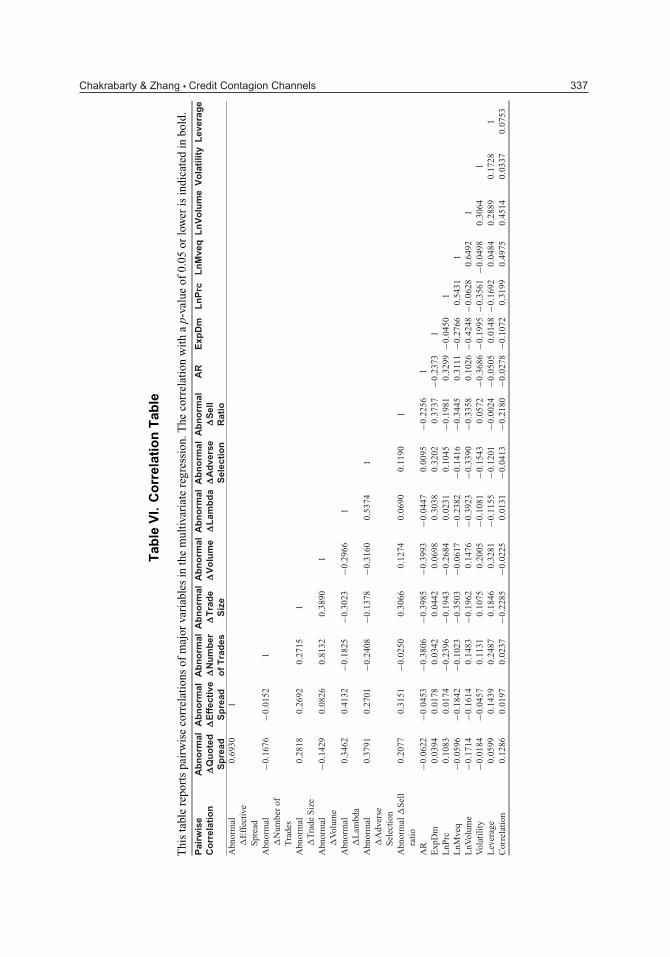
Table VI presents the correlations between our abnormal liquidity measures (dependent vari-ables) and the independent variables used in the regression framework. Coefficients that are sig-nificant at the 95% confidence level or higher are boldfaced. As expected, the liquidity variablesdisplay a high degree of correlation amongst them. For example, abnormal trading volume andnumber of trades have a correlation of greater than 80%, whereas higher trading volume re-duces the price impact of trade, leading to a significant negative correlation between volume andlambda.

The relationships between the explanatory variables are also as expected. For example, highpriced stocks are usually from high market capitalization firms (correlation coefficient = 0.54and significant). The correlation of the equity returns of sample firms with Lehman’s equityreturn is higher for the higher market capitalization firms (correlation coefficient = 0.49 andsignificant).

Because Table VI demonstrates a fair degree of correlation amongst the explanatory variables,we test for potential multicollinearity issues using the variance inflation factor (VIF). All VIFsare below four, suggesting that multicollinearity is not a serious concern for our models.

To address whether a two stage least squares (2SLS) estimation is preferable to the ordinaryleast squares (OLS) procedure, we perform a Hausman test and find no basis to reject the nullhypothesis that OLS is superior to a 2SLS estimation.19 Therefore, we estimate OLS regressions,where the t-statistics for the regression coefficients are based on robust standard errors adjustedfor events clustering. The results are presented in Table VII.

Although the exposure dummy is insignificant in Models 1, 2, 3, and 5, in the other four regres-sion models (6, 7, 8, and 9), this variable is significant and has the right sign. Like the univariateresults presented earlier, these results also bear mixed support for the information transmissionhypothesis. Consistent with the counterparty contagion hypothesis, the exposure dummy is posi-tively associated with abnormal changes in lambda, adverse selection, and sell ratio, all of whichare statistically significant at 5% or above. In Model 9, where the abnormal equity return is thedependent variable, ExpDm is negative and statistically significant. Taken together, the univariateand multivariate results provide strong support for the significance of counterparty contagionrisk because exposed firms experience significantly more negative consequences from Lehman’sbankruptcy, as evidenced by the greater price impact of trade, more information asymmetry,greater selling order imbalance, and considerably lower equity returns than unexposed firms.

IV. Robustness Checks

As detailed in the sample selection procedures, our results are based on the sample of financialfirms (SIC Code 6XXX) that should have the strongest ties to Lehman Brothers. However, Table I

18 To save space, the coefficients on these variables are not reported, but we verify that the estimates have the expectedsigns.19 In addition, we also check for autocorrelation in the dependent variables by doing a Durbin–Watson (DW) test. All theDW test statistics are close to two, indicating no concerns for autocorrelation. The results of the Hausman test and theDW test are available upon request.


Tab

leV

I.C

orr

elat

ion

Tab

le

Thi

sta

ble

repo

rts

pair

wis

eco

rrel

atio

nsof

maj

orva

riab

les

inth

em

ultiv

aria

tere

gres

sion

.The

corr

elat

ion

wit

ha

p-va

lue

of0.

05or

low

eris

indi

cate

din

bold

.P

airw

ise

Ab

no

rmal

Ab

no

rmal

Ab

no

rmal

Ab

no

rmal

Ab

no

rmal

Ab

no

rmal

Ab

no

rmal

Ab

no

rmal

AR

Exp

Dm

Ln

Prc

Ln

Mve

qL

nV

olu

me

Vo

lati

lity

Lev

erag

eC

orr

elat

ion

�Q

uo

ted

�E

ffec

tive

�N

um

ber

�T

rad

e�

Vo

lum

e�

Lam

bd

a�

Ad

vers

e�

Sel

lS

pre

adS

pre

ado

fT

rad

esS

ize

Sel

ecti

on

Rat

ioA

bnor

mal

�E

ffec

tive

Spr

ead

0.69

301

Abn

orm

al�

Num

ber

ofT

rade

s

−0.1

676

−0.0

152

1

Abn

orm

al�

Tra

deS

ize

0.28

180.

2692

0.27

151

Abn

orm

al�

Vol

ume

−0.1

429

0.08

260.

8132

0.38

901

Abn

orm

al�

Lam

bda

0.34

620.

4132

−0.1

825

−0.3

023

−0.2

966

1

Abn

orm

al�

Adv

erse

Sel

ecti

on

0.37

910.

2701

−0.2

408

−0.1

378

−0.3

160

0.53

741

Abn

orm

al�

Sel

lra

tio

0.20

770.

3151

−0.0

250

0.30

660.

1274

0.06

900.

1190

1

AR

−0.0

622

−0.0

453

−0.3

806

−0.3

985

−0.3

993

−0.0

447

0.00

95−0

.225

61

Exp

Dm

0.03

940.

0178

0.03

420.

0442

0.06

980.

3038

0.32

020.

3737

−0.2

373

1L

nPrc

0.10

830.

0174

−0.2

396

−0.1

943

−0.2

684

0.02

310.

1045

−0.1

981

0.32

99−0

.045

01

LnM

veq

−0.0

596

−0.1

842

−0.1

023

−0.3

503

−0.0

617

−0.2

382

−0.1

416

−0.3

445

0.31

11−0

.276

60.

5431

1L

nVol

ume

−0.1

714

−0.1

614

0.14

83−0

.196

20.

1476

−0.3

923

−0.3

390

−0.3

358

0.10

26−0

.424

8−0

.062

80.

6492

1V

olat

ilit

y−0

.018

4−0

.045

70.

1131

0.10

750.

2005

−0.1

081

−0.1

543

0.05

72−0

.368

6−0

. 199

5−0

.356

1−0

.049

80.

3064

1L

ever

age

0.05

990.

1439

0.24

870.

1846

0.32

81−0

.115

5−0

.120

1−0

.002

4−0

.050

50.

0148

−0.1

692

0.04

840.

2889

0.17

281

Cor

rela

tion

0.12

860.

0197

0.02

37−0

.228

5−0

.022

50.

0131

−0.0

413

−0.2

180

−0.0

278

−0.1

072

0.31

990.

4975

0.45

140.

0337

0.07

53

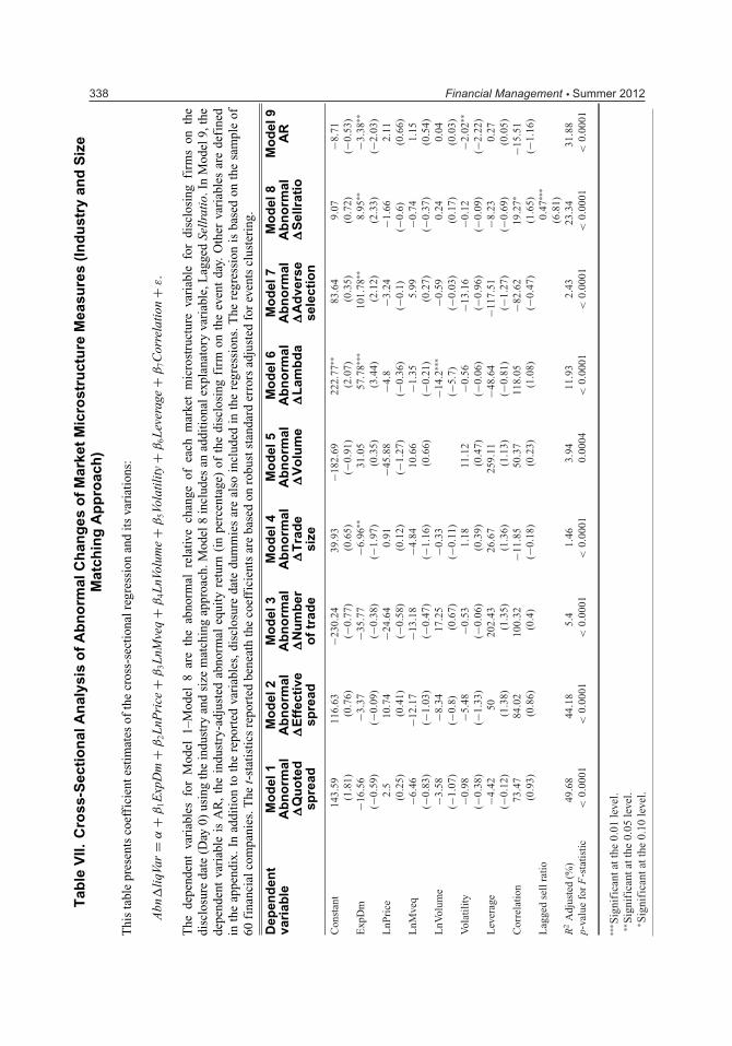
338 Financial Management � Summer 2012T

able

VII.

Cro

ss-S

ecti

on

alA

nal

ysis

of

Ab

no

rmal

Ch

ang

eso

fM

arke

tM

icro

stru

ctu

reM

easu

res

(In

du

stry

and

Siz

eM

atch

ing

Ap

pro

ach

)

Thi

sta

ble

pres

ents

coef

fici

ente

stim

ates

ofth

ecr

oss-

sect

iona

lreg

ress

ion

and

its

vari

atio

ns:

Abn

�li

qVar

=α

+β

1E

xpD

m+

β2L

nPri

ce+

β3L

nMve

q+

β4L

nVol

ume

+β

5Vo

lati

lity

+β

6L

ever

age

+β

7C

orre

lati

on+

ε.

The

depe

nden

tva

riab

les

for

Mod

el1–

Mod

el8

are

the

abno

rmal

rela

tive

chan

geof

each

mar

ket

mic

rost

ruct

ure

vari

able

for

disc

losi

ngfi

rms

onth

edi

sclo

sure

date

(Day

0)us

ing

the

indu

stry

and

size

mat

chin

gap

proa

ch.M

odel

8in

clud

esan

addi

tion

alex

plan

ator

yva

riab

le,L

agge

dSe

llra

tio.

InM

odel

9,th

ede

pend

ent

vari

able

isA

R,

the

indu

stry

-adj

uste

dab

norm

aleq

uity

retu

rn(i

npe

rcen

tage

)of

the

disc

losi

ngfi

rmon

the

even

tda

y.O

ther

vari

able

sar

ede

fine

din

the

appe

ndix

.In

addi

tion

toth

ere

port

edva

riab

les,

disc

losu

reda

tedu

mm

ies

are

also

incl

uded

inth

ere

gres

sion

s.T

here

gres

sion

isba

sed

onth

esa

mpl

eof

60fi

nanc

ialc

ompa

nies

.The

t-st

atis

tics

repo

rted

bene

ath

the

coef

fici

ents

are

base

don

robu

stst

anda

rder

rors

adju

sted

for

even

tscl

uste

ring

.

Dep

end

ent

Mo

del

1M

od

el2

Mo

del

3M

od

el4

Mo

del

5M

od

el6

Mo

del

7M

od

el8

Mo

del

9va

riab

leA

bn

orm

alA

bn

orm

alA

bn

orm

alA

bn

orm

alA

bn

orm

alA

bn

orm

alA

bn

orm

alA

bn

orm

alA

R�

Qu

ote

d�

Eff

ecti

ve�

Nu

mb

er�

Tra

de

�V

olu

me

�L

amb

da

�A

dve

rse

�S

ellr

atio

spre

adsp

read

of

trad

esi

zese

lect

ion

Con

stan

t14

3.59

116.

63−2

30.2

439

.93

−182

.69

222.

77∗∗

83.6

49.

07−8

.71

(1.8

1)(0

.76)

(−0.

77)

(0.6

5)(−

0.91

)(2

.07)

(0.3

5)(0

.72)

(−0.

53)

Exp

Dm

−16.

56−3

.37

−35.

77−6

.96∗∗

31.0

557

.78∗∗

∗10

1.78

∗∗8.

95∗∗

−3.3

8∗∗

(−0.

59)

(−0.

09)

(−0.

38)

(−1.

97)

(0.3

5)(3

.44)

(2.1

2)(2

.33)

(−2.

03)

LnP

rice

2.5

10.7

4−2

4.64

0.91

−45.

88−4

.8−3

.24

−1.6

62.

11(0

.25)

(0.4

1)(−

0.58

)(0

.12)

(−1.

27)

(−0.

36)

(−0.

1)(−

0.6)

(0.6

6)L

nMve

q−6

.46

−12.

17−1

3.18

−4.8

410

.66

−1.3

55.

99−0

.74

1.15

(−0.

83)

(−1.

03)

(−0.

47)

(−1.

16)

(0.6

6)(−

0.21

)(0

.27)

(−0.

37)

(0.5

4)L

nVol

ume

−3.5

8−8

.34

17.2

5−0

.33

−14.

2∗∗∗

−0.5

90.

240.

04(−

1.07

)(−

0.8)

(0.6

7)(−

0.11

)(−

5.7)

(−0.

03)

(0.1

7)(0

.03)

Vol

atil

ity

−0.9

8−5

.48

−0.5

31.

1811

.12

−0.5

6−1

3.16

−0.1

2−2

.02∗∗

(−0.

38)

(−1.

33)

(−0.

06)

(0.3

9)(0

.47)

(−0.

06)

(−0.

96)

(−0.

09)

(−2.

22)

Lev

erag

e−4

.42

5020

2.43

26.6

725

9.11

−48.

64−1

17.5

1−8

.23

0.27

(−0.

12)

(1.3

8)(1

.35)

(1.3

6)(1

.13)

(−0.

81)

(−1.

27)

(−0.

69)

(0.0

5)C

orre

lati

on73

.47

84.0

210

0.32

−11.

8550

.37

118.

05−8

2.62

19.2

7∗−1

5.51

(0.9

3)(0

.86)

(0.4

)(−

0.18

)(0

.23)

(1.0

8)(−

0.47

)(1

.65)

(−1.

16)

Lag

ged

sell

rati

o0.

47∗∗

∗

(6.8

1)R

2A

djus

ted

(%)

49.6

844

.18

5.4

1.46

3.94

11.9

32.

4323

.34

31.8

8p-

valu

efo

rF

-sta

tist

ic<

0.00

01<

0.00

01<

0.00

01<

0.00

010.

0004

<0.

0001

<0.

0001

<0.

0001

<0.

0001

∗∗∗ S

igni

fica

ntat

the

0.01

leve

l.∗∗

Sig

nifi

cant

atth

e0.

05le

vel.

∗ Sig

nifi

cant

atth

e0.

10le

vel.


reports that several (26) nonfinancial firms also made voluntary declarations about their exposure(or lack thereof) to Lehman in the immediate aftermath of its bankruptcy. As a robustness check,we rerun all of our tests using both the financial and nonfinancial firms. We do this because mosttheories of financial contagion relate the effects of a shock (in our case the collapse of LehmanBrothers) to other firms in the economy (not limited to the same industry).

The counterparty hypothesis predicts that the shock from the collapse of a big firm shouldimpact firms that have a direct counterparty relationship with it. The hypothesis makes nodistinction whether such counterparty firms should belong to the same industry. For example,Dynegy, an electric energy production company (SIC Code 1311), had a $70 million LehmanBrothers Commercial Paper commitment under a $1.15 billion revolving credit facility andanother $850 million letter of credit facility. The stock price of Dynegy plunged by over 10%upon its announcement of exposure to Lehman. Although Dynegy is not in the same industry asLehman, its stock price decline reflects a potential loss from having to reestablish these contractswith other financial institutions.

Likewise, the information transmission hypothesis posits that the collapse induces a beliefrevision by all traders, leading to greater trading activities that should impact all firms in theeconomy. Although it is true that the policy implications of the contagion effect pertains topredominantly financial firms, the theoretical predictions (that we test) do not limit contagioneffects to financial firms only. Therefore, the robustness tests should help to relate our work morebroadly to the literature on contagion.

All our conclusions hold in this larger sample. We find mixed support for the informationtransmission hypothesis and strong support for the counterparty risk hypothesis. The univariateresults indicate that although there is liquidity deterioration for both groups, the exposed firmssuffer far worse effects than the unexposed firms. Multivariate results confirm that the exposuredummy variable is significant in four of the nine models. We also run the tests by matching onindustry, market capitalization, and book-to-market (instead of the ISM), and all our results holdin this set of tests, as well.20

V. Conclusion

Lehman was the only large financial institution that filed for bankruptcy during the recentfinancial crisis. Immediately after Lehman’s bankruptcy, over a hundred companies disclosed theirfinancial exposure to Lehman. This allows us to test the significance of credit contagion effectsarising from the collapse of a large financial institution and distinguish two contagion channelsby explicitly controlling for a counterparty relationship. Prior empirical evidence supportinginformation contagion theory does not account for possible counterparty relationships.

A novelty of this study is that we construct microstructure liquidity variables using highfrequency intraday data to provide a finer test of contagion theories. Specifically, our investigationfocuses on the adverse impact on market liquidity, trading activity, information asymmetry, andorder imbalance of other companies because of the financial distress of Lehman Brothers. Ouranalysis contributes to the credit contagion literature by testing contagion effects from a marketmicrostructure perspective.

After controlling for counterparty relationships, we find that the disclosing firms in our sampleexperience liquidity deterioration in some dimensions, providing mixed support for the informa-tion transmission theory. However, our results demonstrate robust evidence for the counterparty

20 All robustness test results are available upon request.


contagion hypothesis. Firms that have exposure to Lehman experience greater decreases in liq-uidity, higher price impacts of trade, and greater increases in information asymmetry. They alsoface greater sell pressure and lower abnormal equity returns than unexposed firms. Therefore,what we might attribute to information-based contagion in the full sample results seems to bedriven mainly by counterparty exposure.

Proper identification of the channels of credit contagion is important from a policy perspective.As argued previously, policy response to financial crises should differ if the channel of contagionis identified as counterparty risk (in which case a bailout of failing financial institutions may berecommended) versus information transmission (in which case supporting the distressed sectormay be a better option). By studying the sources of contagion effects after Lehman’s collapse,our study also contributes to the policy debate on government response to the failure of largefinancial institutions during a financial crisis.

Appendix: Variable Definitions

Name Definition

Microstructure liquidity variablesQuoted Spread Equally weighted quoted bid-ask spreadEffective Spread Equally weighted effective bid-ask spreadNumber of Trades Daily average number of tradesTrade Size Average trade sizeVolume Average daily trading volume in (‘000)LnVolume Natural logarithm of trading volumeLambda (in ‘000) Kyle’s LambdaAdverse Selection (in ‘000) Adverse selection component of bid-ask spreadSellratio (%) Selling ratio (number of seller initiated trades divided by total

trade)Lagged sellratio (%) Lagged selling ratio (number of seller initiated trades divided by

total trade) for the previous dayControl Variables

Price The average stock price in control period (August 2008)LnPrice Natural logarithm of stock priceMveq (in millions) Market value of equity preceding the eventLnMveq Natural logarithm of market value of equityVolatility Daily stock return volatility over the previous yearLeverage The average leverage ratio over four quarters during the preceding

year, defined as the ratio of book value of debt over the marketvalue of assets, taken as the market value of equity plus thebook value of debt

Correlation The correlation of equity returns between the sample firm andLehman Brothers over the preceding year

ExpDm Dummy variable equal to one if the firm has exposure to Lehmanand zero otherwise

References

Ahn, H.J., C. Cao, and H. Choe, 2001, “Share Repurchase Tender Offers and Bid-Ask Spreads,” Journal ofBanking and Finance 25, 445-478.


Anderson, J., E. Dash, V. Bajaj, and E. Andrews, 2008, “US Gives Banks Urgent Warning to Solve Crisis,”The New York Times September 13.

Aragon, G.O. and P.E. Strahan, 2011, “Hedge Funds as Liquidity Providers: Evidence from LehmanBankruptcy,” Journal of Financial Economics, forthcoming.

Bessembinder, H., 1999, “Trade Execution Costs on NASDAQ and the NYSE: A Post-Reform Comparison,”Journal of Financial and Quantitative Analysis 34, 387-407.

Bessembinder, H., 2003, “Issues in Assessing Trade Execution Costs,” Journal of Financial Markets 6,233-257.

Boissay, F., 2006, “Credit Chains and the Propagation of Financial Distress,” European Central Bank,Working Paper.

Bollen, N.P.B., T. Smith, and R.E. Whaley, 2004, “Modeling the Bid/Ask Spread: Measuring the Inventory-Holding Premium,” Journal of Financial Economics 72, 97-141.

Butler, A.W., G. Grullon, and J.P. Weston, 2005, “Stock Market Liquidity and the Cost of Issuing Equity,”Journal of Financial and Quantitative Analysis 40, 331-348.

Calvo, G., 1999, “Contagion in Emerging Markets: When Wall Street Is a Carrier,” University of Maryland,Working Paper.

Chakrabarty, B., P.C. Moulton, and A.A. Shkilko, 2011, “Short Sales, Long Sales, and the Lee-Ready TradeClassification Algorithm,” Cornell University, Working Paper.

Chordia, T., R. Roll, and A. Subrahmanyam, 2002, “Order Imbalance, Liquidity and Market Returns,”Journal of Financial Economics 65, 111-130.

Chung, K., B. Van Ness, and R. Van Ness, 2001, “Can the Treatment of Limit Orders Reconcile the Dif-ferences in Trading Costs between NYSE and NASDAQ Issues?” Journal of Financial and QuantitativeAnalysis 36, 267-286.

Collin-Dufresne, P., R. Goldstein, and J. Helwege, 2010, “Are Jumps in Corporate Bond Yields Priced?Modeling Contagion via the Updating of Beliefs,” NBER, Working Paper.

Corwin, S. and M. Lipson, 2000, “Order Flow and Liquidity Around NYSE Trading Halts,” Journal ofFinance 55, 1771-1801.

Das, S., D. Duffie, N. Kapadia, and L. Saita, 2007, “Common Failings: How Corporate Defaults areCorrelated,” Journal of Finance 62, 93-117.

Davies, R. and S. Kim, 2009, “Using Matched Samples to Test for Differences in Trade Execution,” Journalof Financial Markets 12, 173-202.

Davis, M. and V. Lo, 2001, “Infectious Defaults,” Quantitative Finance 1, 382-387.

Dudley, E. and M. Nimalendran, 2011, “Margins and Hedge Fund Contagion,” Journal of Financial andQuantitative Analysis 46, 1227-1257.

Duffie, D., A. Eckner, G. Horel, and L. Saita, 2009, “Frailty Correlated Default,” Journal of Finance 64,2089-2123.

Easley, D., M. O’Hara, and G. Saar, 2001, “How Stock Splits Affect Trading: A Microstructure Approach,”Journal of Financial and Quantitative Analysis 36, 25-51.

Eberhart, A.C., E.I. Altman, and R. Aggarwal, 1999, “The Equity Performance of Firms Emerging fromBankruptcy,” Journal of Finance 54, 1855-1868.


Fernando, C., A. May, and W. Megginson, 2011, “The Value of Investment Banking Relationships: Evidencefrom the Collapse of Lehman Brothers,” Journal of Finance forthcoming.

Giesecke, K., 2004, “Correlated Default with Incomplete Information,” Journal of Banking and Finance28, 1521-1545.

Giesecke, K. and S. Weber, 2004, “Cyclical Correlations, Credit Contagion, and Portfolio Losses,” Journalof Banking and Finance 25, 3009-3036.

Glosten, L.R. and L.E. Harris, 1988, “Estimating the Components of the Bid/Ask Spread,” Journal ofFinancial Economics 21, 123-142.

Glosten, L.R. and P. Milgrom, 1985, “Bid, Ask and Transaction Prices in a Specialist Market with Hetero-geneously Informed Traders,” Journal of Financial Economics 14, 71-100.

Graham, J.R., S. Li, and J. Qiu, 2008, “Corporate Misreporting and Bank Loan Contracting,” Journal ofFinancial Economics 89, 44-61.

Helwege, J., 2010, “Financial Firm Bankruptcy and Systemic Risk, Journal of International FinancialMarkets, Institutions and Money 20, 1-12.

Inci, A.C., B. Lu, and H.N. Seyhun, 2010, “Intraday Behavior of Stock Prices and Trades Around InsiderTrading,” Financial Management 39, 323-363.

Ivashina, W. and D. Scharfstein, 2010, “Bank Lending During the Financial Crisis of 2008,” Journal ofFinancial Economics 97, 319-338.

Iyer, R. and J.L. Peydro, 2011, “Interbank Contagion at Work: Evidence from a Natural Experiment,” Reviewof Financial Studies 24, 1337-1377.

Jakob K. and T. Ma, 2003, “Order Imbalance on Ex-Dividend Days,” Journal of Financial Research 26,65-75.

Jennings, R., 1994, “Intraday Changes in Target Firms’ Share Price and Bid-Ask Quotes Around TakeoverAnnouncements,” Journal of Financial Research 2, 255-270.

Jorion, P. and G. Zhang, 2007, “Good and Bad Credit Contagion: Evidence from Credit Default Swaps,”Journal of Financial Economics 84, 860-883.

Jorion, P. and G. Zhang, 2009, “Credit Contagion from Counterparty Risk,” Journal of Finance 64, 2053-2087.

Jorion, P. and G. Zhang, 2011, “Financial Contagion and Lehman Brothers’ Bankruptcy,” University ofCalifornia, Irvine, Working Paper.

King, M.A. and S. Wadhwani, 1990, “Transmission of Volatility Between Stock Markets,” Review ofFinancial Studies 3, 5-33.

King, M.R., 2009, “Prebid Run-Ups Ahead of Canadian Takeovers: How Big Is the Problem?” FinancialManagement 38, 699-726.

Krinsky, I. and J. Lee, 1996, “Earnings Announcements and the Components of the Bid-Ask Spread,”Journal of Finance 51, 1523-1535.

Kryzanowski, L., S. Lazrak, and I. Rakita, 2010, “Behavior of Liquidity and Returns Around CanadianSeasoned Equity,” Journal of Banking and Finance 34, 2954-2967.

Kyle, A.S., 1985, “Continuous Auctions and Insider Trading,” Econometrica 53, 1315-1335.

Lang, L. and R.M. Stulz, 1992, “Contagion and Competitive Intra-Industry Effects of BankruptcyAnnouncements,” Journal of Financial Economics 32, 45-60.


Lee, C.M.C. and M.J. Ready, 1991, “Inferring Trade Direction from Intraday Data,” Journal of Finance 46,733-747.

MacKinlay, A.C., 1997, “Event Studies in Economics and Finance,” Journal of Economic Literature 35,13-39.

Massa, M. and A. Simonov, 2005, “Is Learning a Dimension of Risk?” Journal of Banking and Finance 29,2605-2632.

Oliver K. and R.E. Verrecchia, 1994, “Market Liquidity and Volume Around Earnings Announcements,”Journal of Accounting and Economics 17, 41-67.

Phylaktis, K. and L. Xia, 2009, “Equity Market Comovement and Contagion: A Sectoral Perspective,”Financial Management 38, 381-409.

Smith, B.F., R. White, M. Robinson, and R. Nason, 1997, “Intraday Volatility and Trading Volume AfterTakeover Announcements,” Journal of Banking and Finance 21, 337-368.

Venkatesh, P.C. and R. Chiang, 1986, “Information Asymmetry and the Dealer’s Bid-Ask Spread: A CaseStudy of Earnings and Dividend Announcements,” Journal of Finance 41, 1098-1102.

White, B. and J. Anderson, 2008, “Lehman Heads Toward Brink as Barclays Ends Talks,” The New YorkTimes, September 14.

Yuan, K., 2005, “Asymmetric Price Movements and Borrowing Constraints: A Rational ExpectationsEquilibrium Model of Crisis, Contagion, and Confusion,” Journal of Finance 60, 379-411.

Documents

Credit Contagion Channels: Market Microstructure Evidence