Credit Default Swap Spreads and Systemic Financial Risk∗

Stefano GiglioHarvard University

JOB MARKET PAPER

January 2011

Abstract

This paper presents a novel method to measure the joint default risk of large financial insti-tutions (systemic default risk) using information in bond and credit default swap (CDS) prices.Bond prices reflect individual default probabilities of the issuers. CDS contracts, which insureagainst such defaults, pay off only as long as the seller of protection itself is solvent. Therefore,CDS prices contain information about the probability of joint default of both the bond issuerand the protection seller. If we consider the entire set of CDS contracts written by each financialinstitution against the default of each other institution we can learn about all pairwise defaultprobabilities across the financial network. This information, however, is not sufficient to com-pletely characterize the joint distribution function of defaults of these banks. In this paper, Ishow how this information can be optimally aggregated to construct bounds on the probabilityof systemic default events. This method enables me to measure systemic default risk withoutmaking any assumptions about the joint distribution function. Two main results emerge fromthe empirical application of this method to the recent financial crisis. First, I show that anincrease in systemic risk in large global banks did not occur until after Bear Stearns’ collapse inMarch 2008. Second, some of the large observed spikes in CDS spreads and bond yield spreadsduring this period (for example, following Lehman Brothers’ default) correspond to spikes inidiosyncratic default risk rather than systemic risk.

∗Contact: sgiglio@fas.harvard.edu. I owe special thanks to Effi Benmelech, John Campbell and Emmanuel Farhifor their many comments and suggestions. Also, I am very grateful to Ruchir Agarwal, Robert Barro, Hui Chen,Josh Coval, Tom Cunningham, Mikkel Davies, Ian Dew-Becker, Ben Friedman, Bob Hall, Eugene Kandel, LeonidKogan, Anton Korinek, David Laibson, Greg Mankiw, Ian Martin, Parag Pathak, Carolin Pfueger, Monika Piazzesi,Martin Schneider, Tiago Severo, Andrei Shleifer, Alp Simsek, Ken Singleton, Holger Spamann, Jeremy Stein, BobTurley, Tom Vogl, Charles-Henri Weymuller and seminar participants at the Harvard Macro Lunch, the HarvardFinance Lunch, the MIT Sloan Finance Lunch, the Stanford Institute for Theoretical Economics and the Program forEvolutionary Dynamics at Harvard for many helpful suggestions.

1 Introduction

This paper seeks to measure the probability that several large financial institutions default withina short time. During periods of financial distress, this probability is not negligible because largefinancial intermediaries are highly interconnected and are exposed to common shocks. The centralrole of these institutions in the global economy makes this issue especially important. In particular,in this paper I focus on measuring the probability of default of at least r large financial institutions.I refer to these joint default events as systemic default risk of degree r.

Measuring systemic risk is a difficult task. On the one hand, measures that are based directly onthe books of financial institutions are mostly backward-looking in nature. They are limited by thecomplexity of the balance sheet, the risks involved and the availability of data. On the other hand,measures based on the historical distribution of returns require estimating joint tail probabilitiesfrom limited time series, which is possible only under strong parametric assumptions.

The most widely used measures of systemic risk, like the one proposed in this paper, are insteadmarket-based. They try to circumvent the limitations outlined above by aggregating individual de-fault probabilities of financial institutions obtained from the prices of traded securities like creditdefault swaps (CDSs).1 These market-based measures are forward-looking and reflect the informa-tion set of market participants; they measure risk-neutral rather than objective default probabilities.

Figure 1 plots two simple examples of such market-based measures of default risk in the financialsector: the average 5-year bond yield spread and the average 5-year CDS spread of the largest 15financial institutions by CDS activity2 between 2004 and 2010. The yield spread (the yield on afirm’s bonds in excess of the risk-free rate) and the CDS spread (the cost of insuring against thefirm’s default) both reflect the probability that a firm defaults. The idea behind these measuresis that an increase in systemic risk in the financial sector should cause the risk of default of eachinstitution to increase. This should result in an increase of both the average yield spread and theaverage CDS spread. These measures suggest an increase in systemic risk starting in August 2007,followed by several episodes in which systemic risk spiked (such as around March 2008, September2008 and then March 2009), and a final drop after April 2009.

The existing market-based measures can be misleading for two reasons. First, they involve strongmodeling assumptions in aggregating the individual risks of financial intermediaries into estimatesof systemic risk. For example, the CDS-based measure reported in Figure 1 is only informativeabout the joint distribution of defaults under strong assumptions about the relationship betweenmarginal and joint default probabilities. Second, existing measures based on the prices of securitiestraded over the counter (OTC) ignore counterparty risk. As I show below, ignoring counterpartyrisk introduces a bias that increases precisely when the financial system is distressed.

In this paper I propose a novel market-based measure of systemic risk, based on a combination1A credit default swap is an insurance contract against the default of a firm, for example a financial institution.

The CDS spread corresponds to the yearly insurance premium. See section 2 for details on the contract.2The Figure replicates the Counterparty Risk Index, produced by Credit Derivative Research. The index was

created to allow buyers of CDS protection to easily hedge their counterparty risk exposures, and therefore includesthe spreads of the most active counterparties in the CDS market. These 15 institutions alone constitute more than90% of the CDS protection sold.

1

of bond prices and CDS spreads. I exploit the pricing of counterparty risk in CDS contracts tolearn about the joint default risk of pairs of institutions. Because this information set is not richenough to completely characterize the full joint distribution function across the network, I use linearprogramming to construct the tightest possible bounds on systemic risk consistent with the observedprices. This allows me to measure systemic risk without making modeling assumptions about therelationship between risks of individual institutions and joint risks. In addition, it allows me to trackthe contribution to systemic risk of each bank over time.

The starting point for the analysis is the presence of counterparty risk in CDS contracts. Whenthe seller of protection manifests higher risk of default, the value of the default insurance (theCDS spread) decreases, particularly if the two defaults are correlated. Therefore, the spread of aCDS written by a financial institution against the default of a bond reflects both the probability ofdefault of the bond issuer, called the reference entity, and the risk of joint default with the sellerof protection. The price of the bond instead reflects only the marginal probability of default of thefirm which issued the bond.3 Combining bond and CDS prices enables us to infer the joint defaultprobability of the two entities.

A standard way to see this is to look at the bond/CDS basis. By buying the bond and insuringit with the corresponding CDS of the same maturity, one obtains a risk-free debt security as long asthere is no counterparty risk in the CDS contract. An approximate arbitrage relation then impliesthat in the absence of counterparty risk, the yield spread on the bond issued by i over the risk-free rate(yi− rF ) should be equal to the corresponding CDS spread zi written on i. That is, the bond/CDSbasis, defined as the difference between the two (zi − (yi − rF )), should be zero. Counterpartyrisk, by lowering the CDS spread zi without affecting the yield spread of the bond, produces anegative basis. The bond/CDS basis therefore contains information about the joint default risk ofthe reference entity and the protection seller. Figure 1 shows that the average bond/CDS basis forfinancial institutions is negative, as expected, and varies significantly over time.

The entire set of bond prices of financial institutions and CDS spreads written on them by otherfinancial institutions allows us to learn all marginal and pairwise probabilities of default across thefinancial network. In general, this information set is not sufficient to completely pin down systemicdefault risk. Standard approaches to measuring systemic risk overcome this problem by imposingmodeling assumptions, such as Gaussian or Student-t copulas, that allow them to obtain pointestimates of the joint default probabilities.

In this paper, instead, I construct the tightest upper and lower bounds on the average monthlyprobability of joint default of at least r financial institutions (for different values of r) consistentwith the observed bond and CDS prices. These bounds are obtained making no assumptions aboutthe joint default distribution and only use marginal and pairwise default information inferred fromsecurity prices. Yet, because they are constructed to be the tightest possible bounds for systemicrisk, they prove to be quite informative about joint default risk.

Three limitations affect the construction of the bounds. First, the presence of an unobserved3Of course, other factors affect bond prices as well. The most important one, liquidity, is explicitly accounted for

in the paper.

2

liquidity process in the bond market confounds the filtering of individual default probabilities outof CDS spreads. Nevertheless, interesting results can be obtained under minimal assumptions onthe liquidity process. In particular, I only impose a lower bound for this process, calibrated fromthe time series of bond and CDS prices of each bank, or from the cross-section of financial andnonfinancial firms of comparable credit rating. Second, for every reference entity, I observe only anaverage of the CDS quotes posted by the main counterparties, so my information set is smaller thanthe ideal one.4 Third, this paper obtains risk-neutral, not objective, default probabilities.5 Therisk-neutral probabilities are interesting per se because they reveal the perception of the marketsabout the severity of these states of the world. In addition, they can be considered upper bounds onthe objective default probabilities, because default states are bad states with high marginal utility.6

Finally, I show strong implications for objective probabilities under mild assumptions on the utilityfunction.

This analysis, applied to the period between January 2004 and June 2010, shows that when weconsider the information contained in both bond and CDS prices, we can bound systemic risk tobe much lower than if we used bond prices or CDS spreads alone. Contrary to other measures ofsystemic risk, which report a sharp increase in systemic risk already in 2007, we can exclude a largeincrease in systemic default risk before Bear Stearns’ failure in March 2008. Moreover, we can showthat observed spikes in CDS spreads and bond yields in the month before Bear’s collapse and inSeptember 2008, after Lehman’s default, do not correspond to spikes in systemic risk (as standardmeasures report), but reflect sharp increases in idiosyncratic default risk of one or a small numberof banks. Instead, systemic risk seems to increase smoothly after an initial jump related to Bear’sfailure.

While the optimal bounds are a complex function of the constraints imposed by the observedprices, the intuition for the main results is straightforward. If systemic risk had been high in 2007and early 2008, the price of insurance against large dealers - purchased from other large financialinstitutions - should have dropped considerably. But this did not happen. The relatively highequilibrium spreads during this period impose a tight upper bound on the amount of systemic riskperceived in financial markets. Equivalently, the bond/CDS basis – which reflects joint default risks– did not increase enough during 2007 and early 2008 to be consistent with an increase in systemicdefault risk. This paper allows for a decomposition between idiosyncratic and systemic default riskthat would be impossible to achieve without the information contained in the basis.

Finally, the methodology presented in this paper allows me to study the configuration of thefinancial network over time, as well as the contribution to systemic risk of each institution at theupper bound on systemic risk. This analysis shows that markets anticipated by more than a montha sharp increase in the joint default probability of two key institutions, Lehman Brothers and MerrillLynch, which in fact ended up facing default on the same weekend (13-14 September 2008). Similarly,

4This limitation is also the reason I look at the group of dealers who are counterparties to most contracts (morethan 90% of the market). This way, I can be confident I am including most of the dealers from whom the CDS quotesare obtained.

5Anderson (2009) underlines the differences between the two by comparing risk-neutral default processes obtainedfrom CDS spreads with objective processes obtained using historical data on defaults.

6This argument assumes that the marginal investor is risk averse and internalizes the risks of these securities.

3

these banks’ contribution to systemic risk (i.e. the probability of a systemic event in which theywould be involved) increased sharply well before their collapse.

The paper proceeds as follows. After a brief literature review, section 2 presents an introductionto credit default swaps and counterparty risk. Section 3 presents the theory of the optimal probabilitybounds, and section 4 discusses the main issues of implementation and the data. Section 5 presentsthe empirical results. In section 6, I run a series of robustness tests. Section 7 concludes.

1.1 Related literature on measuring systemic risk

The literature on measures of systemic risk in the financial sector is large and has grown furtherfollowing the financial crisis of 2007-2009. Four categories of papers can be identified, based ondifferent methods they use to quantify systemic risk and to study the relative contribution of eachbank to this risk.

First, structural approaches look directly at the books of financial institutions in order to learnabout the distribution of joint shocks. Lehar (2005) uses the Merton (1974) model to obtain thetime-series of the market value of banks’ assets, using observed equity prices and balance sheetinformation. He produces a measure of joint default risk under the assumption of multivariatenormal distribution of returns. Gray et al. (2008) propose using a similar approach to measuresystemic risk not only within the financial sector but also across sectors and countries.

The structural approach requires strong assumptions about the liability structure of financialinstitutions, as well as about the marginal and joint distribution of risks. To overcome these difficul-ties, reduced-form approaches look at the historical distribution of returns. For example, Acharyaet al. (2010) compute a measure of individual contributions to systemic risk from individual banks’equity returns during periods of negative returns for the financial sector as a whole. Similarly, Adrianand Brunnermeier (2009) use quantile regression to estimate the VaR of the financial sector as awhole conditional on each individual bank experiencing a loss in its asset values.

A reduced-form approach looking at historical returns has the disadvantage of trying to learnabout tail events from a limited time series of returns. This requires strong assumptions about thetail behavior of return distributions. A third branch of the literature tries to avoid this problem bylooking directly at the probabilities of tail risks implied by derivatives whose price is very sensitive tothese precise risks. Lacking a traded security that directly reflects the joint default risk of the largestfinancial institutions, papers in this category typically extract marginal default risk information fromCDS spreads, and make inference about joint default risk by aggregating them using a certain copulatogether with estimates of correlations. Examples are Huang, Zhou and Zhu (2009) and Avesani,Pascual and Li (2006), which assume Normal and Student-t copulas, and Segoviano and Goodhart(2009), which employs the CIMDO copula (Segoviano (2008)). These papers estimate a time-seriesof systemic risk that closely resembles the simple measures plotted in Figure 1, with large spikesaround March and September 2008 and a steep increase in systemic risk starting in August 2007.These results are in sharp contrast with the ones presented in this paper, which does not need toassume any specific copula for the joint distribution of defaults but uses all the information in bondand CDS prices to learn about pairwise default risk.

4

Finally, several other papers have proposed measures of systemic risk that do not result inestimates of joint default risks. For example, Kritzman, Li, Page and Rigobon (2010) propose usingthe fraction of the variance explained by the first principal components of CDS spreads of largefinancial institutions as a measure of systemic risk in the financial sector. Other papers, instead, useindividual or aggregated financial indicators to empirically predict financial crises, often in a cross-country setting. Examples of this approach are Poghoshan and Cihak (2009), Cihak and Schaeck(2007), Demirguc and Detragiache (1998 and 1999), and Gonzales-Hermosillo (1999).

2 Credit Default Swaps and Counterparty Risk

This section discusses the sources of counterparty risk in CDS contracts. I first describe the maincharacteristics of CDS contracts. Then, I discuss why counterparty risk in these contracts arisesmainly from the possibility of double default of the reference entity and the counterparty. This riskcan be sizable if defaults of financial institutions are not independent. Finally, I argue that collateralprovisions, when present, are unlikely to eliminate this risk. Therefore, counterparty risk should bepriced in CDS spreads.

2.1 The Credit Default Swaps Market

Credit default swaps are credit derivatives that allow the transfer of the credit risk of a firm betweentwo agents for a predetermined amount of time. In a typical CDS contract, the protection seller offersthe protection buyer insurance against the default of an underlying bond issued by a certain company(the reference entity). In the event of default by the reference entity, the seller commits to buy thebond for a price equal to its face value from the protection buyer.7 In exchange for the insurance,the buyer pays a quarterly premium, called the CDS spread, quoted as an annualized percentage ofthe notional value insured. If default occurs, the contract terminates, and the quarterly paymentsare interrupted. If default does not occur during the life of the contract, the contract terminates atits maturity date.

While in general these contracts are traded over the counter and can be customized by the buyerand the seller, in the recent years they have become more standardized, following the guidelines ofthe International Swaps and Derivatives Association (ISDA). The CDS market is quite liquid, withlow transaction costs to initiate a contract with a market maker on short notice, and with numerousdealers posting quotes (see Blanco et al. (2003) and Longstaff et al. (2005)). Reliable quotes for the5-year maturity CDS can be obtained through several financial data firms (Bloomberg, Datastream,Markit).

The CDS market has grown quickly in the last few years. Notional exposures grew from about$5 trillion in 2004 to around $60 trillion at its peak in 2007, and despite the financial crisis, the total

7In practice, the terms of the CDS could involve physical delivery of the defaulted bond or cash settlement. Inthe former case, usually any bond of equal seniority can be delivered. For example, for the CDS written on a seniorunsecured bond, any other senior unsecured bond of the firm could be delivered. In addition, the credit event couldinclude restructuring or a downgrade of the reference bond. These clauses have a potential effect on the price of theCDS, discussed in Appendix C.

5

notional exposure is still around $40 trillion. The main reason for this growth in gross terms is that,due to the high liquidity of the CDS market, the easiest way to adjust the exposure to credit riskhas been to enter new CDS contracts (possibly offsetting the existing ones) rather than operatingdirectly in the bond market or cancelling CDS agreements already in place. At the center of thisnetwork of CDS contracts, a few main dealers operated with very high gross and low net exposures,emerging as the main counterparties in the market. For example, Fitch Ratings8 states that in2006 the top 10 counterparties (all broker/dealers) accounted for about 89% of the total protectionsold. With the crisis, the market concentrated even more, after the disappearance of some of its keyplayers.9

2.2 Counterparty Risk

Traded over the counter, a CDS contract involves counterparty risk: the protection seller mightdefault during the life of the CDS and therefore might not be able to comply with the commitmentsimplied by the contract.10 In this case, the holders of CDS claims would still recover part of theexpected payments due under the contract. Like other derivatives, CDS claims are treated paripassu with senior unsecured bonds, but they are also protected by “safe harbor” provisions, whichexempt them from automatic stay of the assets of the firms, so that they can immediately seize anycollateral that has been posted for them. In addition, positions across different derivatives with thesame counterparty can be netted against each other. The latter potentially increases the recovery incase of counterparty default, but only if the buyer finds herself with large enough out-of-the-moneypositions with the seller when the seller defaults, thus hedging counterparty risk.11

In the case of early termination of the contract due to seller default, the seller has to compensatethe buyer for the replacement cost of the contract, i.e. the cost of initiating a new insurance contractwith another protection seller. This claim is small as long as the default risk of the reference entitydoes not jump substantially when the seller defaults, relative to the original terms of the contract.The larger the change in the CDS spread of the reference entity when the seller defaults, the largerthe claim of the buyer against the defaulted counterparty. In the extreme case, where the default ofthe seller occurs simultaneously with the default of the reference entity, the payment due under thecontract would be equal to the full insurance payment.

A simple two-period example of the pricing of bonds and CDSs can be useful to understand therole of counterparty risk. Consider a group of N dealers which have each issued a zero-coupon bondwith a face value of $1 maturing at time 1, and the CDS contract written at time 0 by each of themagainst the default of each other dealer. Call Ai the event of default of institution i at time 1. CallP (Ai) the probability of default of bank i, and P (Ai ∩Aj) the probability of joint default of i and j

8Fitch Ratings, 2006, Global Credit Derivatives Survey.9Fitch Ratings, 2008, Global Credit Derivatives Survey.

10The role of counterparty risk in CDS spreads has been studied by Hull and White (2001), Jarrow and Turnbull(1995), Jarrow and Yu (2001), and more recently, in the context of rare disaster risk, by Barro (2010). To reducecounterparty risk - which stems mainly from the OTC nature of the contract - there are now several proposal to createa centralized clearinghouse. For a detailed discussion, see Duffie and Zhu (2010).

11The possibility of entering offsetting contracts with the counterparty, rather than canceling existing ones, willwork in this direction.

6

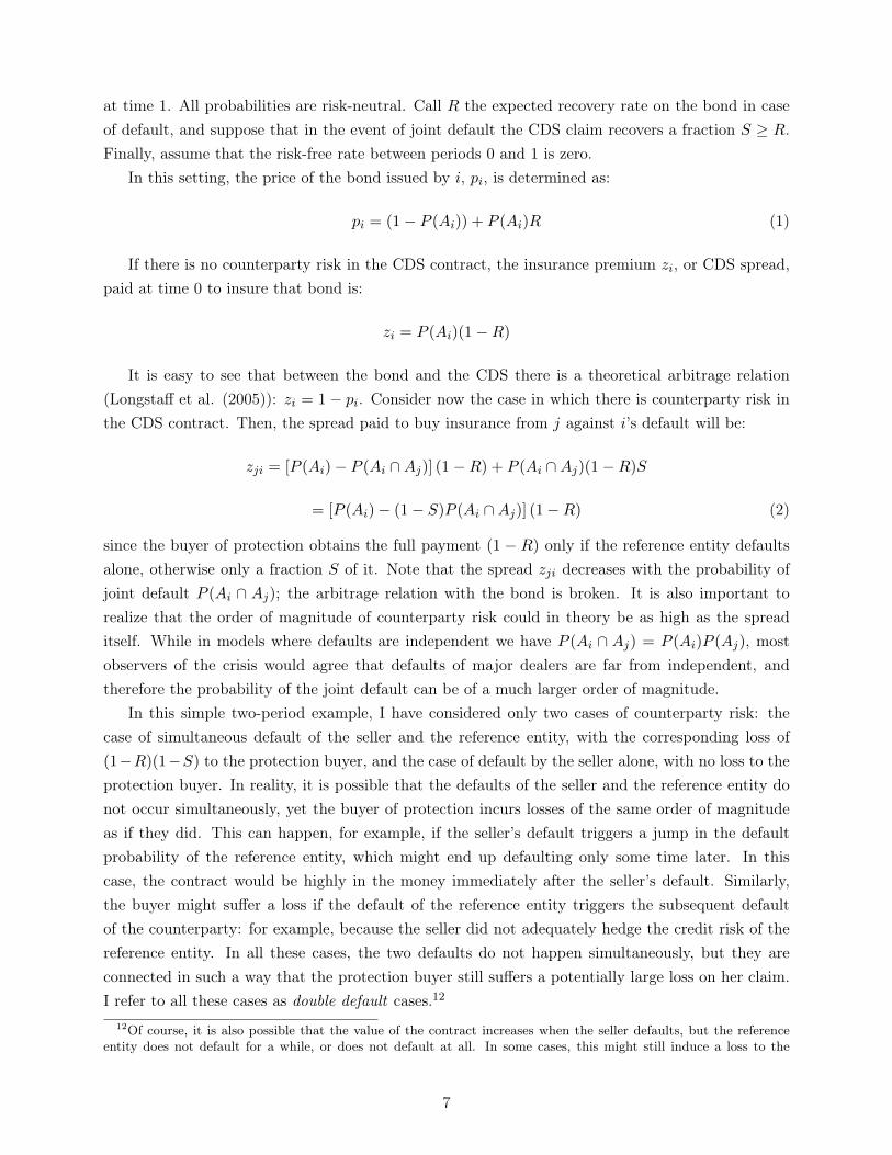
at time 1. All probabilities are risk-neutral. Call R the expected recovery rate on the bond in caseof default, and suppose that in the event of joint default the CDS claim recovers a fraction S ≥ R.Finally, assume that the risk-free rate between periods 0 and 1 is zero.

In this setting, the price of the bond issued by i, pi, is determined as:

pi = (1− P (Ai)) + P (Ai)R (1)

If there is no counterparty risk in the CDS contract, the insurance premium zi, or CDS spread,paid at time 0 to insure that bond is:

zi = P (Ai)(1−R)

It is easy to see that between the bond and the CDS there is a theoretical arbitrage relation(Longstaff et al. (2005)): zi = 1− pi. Consider now the case in which there is counterparty risk inthe CDS contract. Then, the spread paid to buy insurance from j against i’s default will be:

zji = [P (Ai)− P (Ai ∩Aj)] (1−R) + P (Ai ∩Aj)(1−R)S

= [P (Ai)− (1− S)P (Ai ∩Aj)] (1−R) (2)

since the buyer of protection obtains the full payment (1 − R) only if the reference entity defaultsalone, otherwise only a fraction S of it. Note that the spread zji decreases with the probability ofjoint default P (Ai ∩ Aj); the arbitrage relation with the bond is broken. It is also important torealize that the order of magnitude of counterparty risk could in theory be as high as the spreaditself. While in models where defaults are independent we have P (Ai ∩ Aj) = P (Ai)P (Aj), mostobservers of the crisis would agree that defaults of major dealers are far from independent, andtherefore the probability of the joint default can be of a much larger order of magnitude.

In this simple two-period example, I have considered only two cases of counterparty risk: thecase of simultaneous default of the seller and the reference entity, with the corresponding loss of(1−R)(1−S) to the protection buyer, and the case of default by the seller alone, with no loss to theprotection buyer. In reality, it is possible that the defaults of the seller and the reference entity donot occur simultaneously, yet the buyer of protection incurs losses of the same order of magnitudeas if they did. This can happen, for example, if the seller’s default triggers a jump in the defaultprobability of the reference entity, which might end up defaulting only some time later. In thiscase, the contract would be highly in the money immediately after the seller’s default. Similarly,the buyer might suffer a loss if the default of the reference entity triggers the subsequent defaultof the counterparty: for example, because the seller did not adequately hedge the credit risk of thereference entity. In all these cases, the two defaults do not happen simultaneously, but they areconnected in such a way that the protection buyer still suffers a potentially large loss on her claim.I refer to all these cases as double default cases.12

12Of course, it is also possible that the value of the contract increases when the seller defaults, but the referenceentity does not default for a while, or does not default at all. In some cases, this might still induce a loss to the

7

2.3 Collateral Agreements and Pricing of Counterparty Risk

In order to protect the buyers against counterparty risk, some (but not all) CDS contracts involve acollateral agreement, under which collateral calls are tied mechanically to changes in the value of theCDS contract, as well as to downgrades of the rating of the protection seller. Typically, margins onCDSs are adjusted at a daily or weekly frequency. While helpful in reducing counterparty exposure,standard collateral agreements cannot eliminate the counterparty risk coming from double default.In this section I discuss the main reasons for this, and I provide additional evidence in Appendix A.

First, according to the ISDA Margin Survey 2008, only about 66% of the nominal exposure incredit derivatives (of which CDSs are the most important type) had a collateral agreement at allin 2007 and 2008; this number was even lower in the years before. In addition, as reported in theISDA Survey, collateral agreements were employed much less frequently when the counterparty wasa large dealer.

Second, several documents reveal that often collateral posted was even lower than the currentvalue of the position. Even the buyer that most aggressively called for collateral during the crisis,Goldman Sachs, was not covered completely on its CDS exposures with other large dealers (inparticular, AIG), let alone the potential exposure in case of sudden default of the reference entities.13

As several documents show, smaller buyers of CDSs had much less collateral posted than the valueof their positions - large dealers were usually able to obtain more collateral than they had to postwhen dealing with smaller counterparties.

Third, the nature of collateral posting is such that even for buyers who call enough collateralto fully cover the current value of their positions, the extent to which counterparty risk is reduceddepends on the jump properties of the default events. As long as defaults are relatively well antici-pated (there are no jumps), adjustment of collateral to the current value of the exposure can removealmost all counterparty risk. However, especially for financial intermediaries, defaults often occursuddenly and over very short periods of time (e.g. over the weekend), so that the buyer might notbe able to obtain enough collateral to cover all the losses in time.

The Lehman bankruptcy is an interesting example of this. Until the weekend of September13th-14th, during which Lehman collapsed and two other large financial institutions were bailedout (Merrill Lynch and AIG), the default risk of these financial institutions was deemed to be low,as reflected by low CDS spreads and high credit ratings. The joint shock to the three institutionshappened suddenly, so that collateral adjustment would have been small. As it turned out, a doubledefault event did not materialize, because of the government bailout - therefore, buyers of Merrilland AIG CDSs from Lehman did not experience large losses. However, these events show thatthe risk of simultaneous collapse of several banks was relevant, and that standard collateralizationpractices would not have prevented large losses to buyers of CDS contracts, had the government

protection buyer. However, as long as the default risk of the reference entity remains of the same order of magnitude,the value of the contract will be sufficiently small that the collateral posted will allow the recovery of most of it. Insection 4 I describe more in detail the exact pricing model I use.

13The documents refer specifically to a large amount ($22bn) of CDS protection bought by Goldman from AIG onsuper-senior tranches of CDOs, but arguably similar practices were used on all credit derivatives instruments.

8

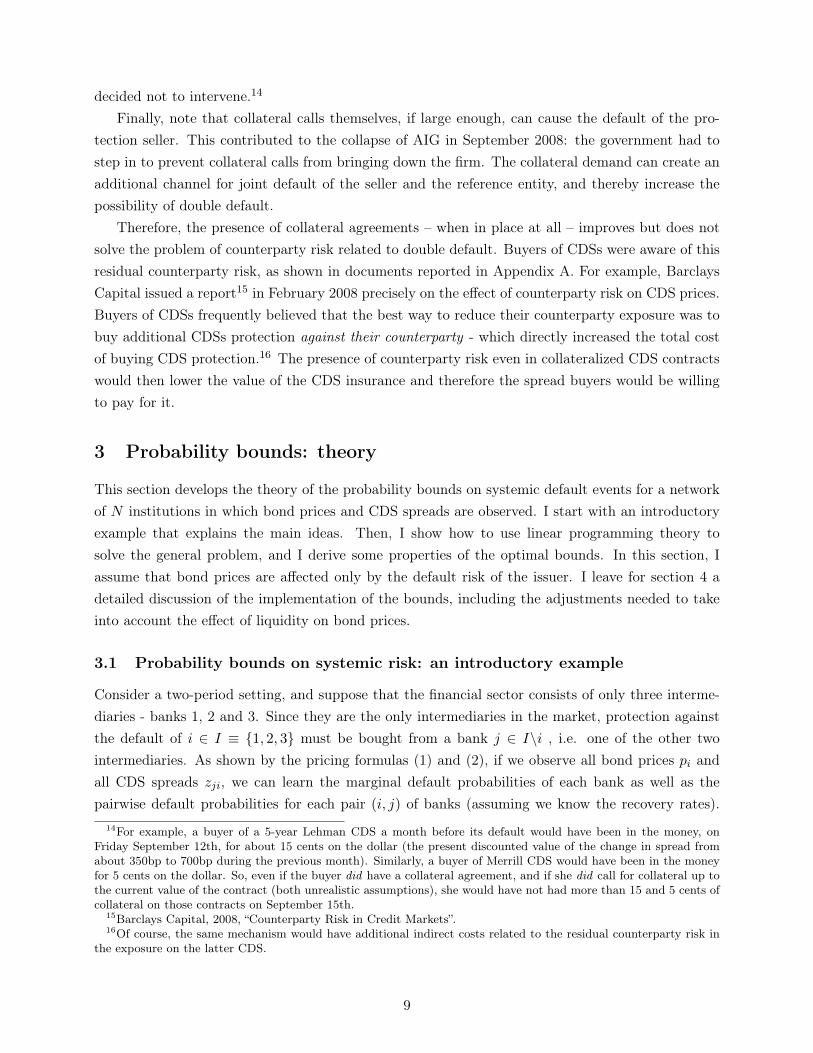
decided not to intervene.14

Finally, note that collateral calls themselves, if large enough, can cause the default of the pro-tection seller. This contributed to the collapse of AIG in September 2008: the government had tostep in to prevent collateral calls from bringing down the firm. The collateral demand can create anadditional channel for joint default of the seller and the reference entity, and thereby increase thepossibility of double default.

Therefore, the presence of collateral agreements – when in place at all – improves but does notsolve the problem of counterparty risk related to double default. Buyers of CDSs were aware of thisresidual counterparty risk, as shown in documents reported in Appendix A. For example, BarclaysCapital issued a report15 in February 2008 precisely on the effect of counterparty risk on CDS prices.Buyers of CDSs frequently believed that the best way to reduce their counterparty exposure was tobuy additional CDSs protection against their counterparty - which directly increased the total costof buying CDS protection.16 The presence of counterparty risk even in collateralized CDS contractswould then lower the value of the CDS insurance and therefore the spread buyers would be willingto pay for it.

3 Probability bounds: theory

This section develops the theory of the probability bounds on systemic default events for a networkof N institutions in which bond prices and CDS spreads are observed. I start with an introductoryexample that explains the main ideas. Then, I show how to use linear programming theory tosolve the general problem, and I derive some properties of the optimal bounds. In this section, Iassume that bond prices are affected only by the default risk of the issuer. I leave for section 4 adetailed discussion of the implementation of the bounds, including the adjustments needed to takeinto account the effect of liquidity on bond prices.

3.1 Probability bounds on systemic risk: an introductory example

Consider a two-period setting, and suppose that the financial sector consists of only three interme-diaries - banks 1, 2 and 3. Since they are the only intermediaries in the market, protection againstthe default of i ∈ I ≡ 1, 2, 3 must be bought from a bank j ∈ I\i , i.e. one of the other twointermediaries. As shown by the pricing formulas (1) and (2), if we observe all bond prices pi andall CDS spreads zji, we can learn the marginal default probabilities of each bank as well as thepairwise default probabilities for each pair (i, j) of banks (assuming we know the recovery rates).

14For example, a buyer of a 5-year Lehman CDS a month before its default would have been in the money, onFriday September 12th, for about 15 cents on the dollar (the present discounted value of the change in spread fromabout 350bp to 700bp during the previous month). Similarly, a buyer of Merrill CDS would have been in the moneyfor 5 cents on the dollar. So, even if the buyer did have a collateral agreement, and if she did call for collateral up tothe current value of the contract (both unrealistic assumptions), she would have not had more than 15 and 5 cents ofcollateral on those contracts on September 15th.

15Barclays Capital, 2008, “Counterparty Risk in Credit Markets”.16Of course, the same mechanism would have additional indirect costs related to the residual counterparty risk in

the exposure on the latter CDS.

9

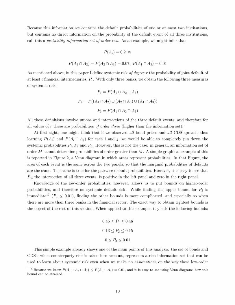
Because this information set contains the default probabilities of one or at most two institutions,but contains no direct information on the probability of the default event of all three institutions,call this a probability information set of order two. As an example, we might infer that

P (Ai) = 0.2 ∀i

P (A1 ∩A2) = P (A2 ∩A3) = 0.07, P (A1 ∩A3) = 0.01

As mentioned above, in this paper I define systemic risk of degree r the probability of joint default ofat least r financial intermediaries, Pr. With only three banks, we obtain the following three measuresof systemic risk:

P1 = P (A1 ∪A2 ∪A3)

P2 = P ((A1 ∩A2) ∪ (A2 ∩A3) ∪ (A1 ∩A3))

P3 = P (A1 ∩A2 ∩A3)

All these definitions involve unions and intersections of the three default events, and therefore forall values of r these are probabilities of order three (higher than the information set).

At first sight, one might think that if we observed all bond prices and all CDS spreads, thuslearning P (Ai) and P (Ai ∩ Aj) for each i and j, we would be able to completely pin down thesystemic probabilities P1, P2 and P3. However, this is not the case: in general, an information set oforderM cannot determine probabilities of order greater thanM . A simple graphical example of thisis reported in Figure 2, a Venn diagram in which areas represent probabilities. In that Figure, thearea of each event is the same across the two panels, so that the marginal probabilities of defaultsare the same. The same is true for the pairwise default probabilities. However, it is easy to see thatP3, the intersection of all three events, is positive in the left panel and zero in the right panel.

Knowledge of the low-order probabilities, however, allows us to put bounds on higher-orderprobabilities, and therefore on systemic default risk. While finding the upper bound for P3 isimmediate17 (P3 ≤ 0.01), finding the other bounds is more complicated, and especially so whenthere are more than three banks in the financial sector. The exact way to obtain tightest bounds isthe object of the rest of this section. When applied to this example, it yields the following bounds:

0.45 ≤ P1 ≤ 0.46

0.13 ≤ P2 ≤ 0.15

0 ≤ P3 ≤ 0.01

This simple example already shows one of the main points of this analysis: the set of bonds andCDSs, when counterparty risk is taken into account, represents a rich information set that can beused to learn about systemic risk even when we make no assumptions on the way these low-order

17Because we know P (A1 ∩ A2 ∩ A3) ≤ P (A1 ∩ A3) = 0.01, and it is easy to see using Venn diagrams how thisbound can be attained.

10

probabilities aggregate at the higher-order level.This example can be used to illustrate two additional concepts related to the measurement of

systemic risk. The first one is that simply averaging the CDS spreads of financial institutions can leadto an erroneous measure of systemic risk. Using the notation introduced above, such a calculationwould measure systemic risk using an index constructed as:

1

6

∑i

∑j 6=i

zij =(1−R)

3

∑i

P (Ai)− (1− S)∑i,j<i

P (Ai ∩Aj)

(3)

Suppose that banks become more correlated (the joint default probabilities increase) while themarginal default probabilities remain the same or increase only slightly. Then, this index in factdecreases. The reason is that, because of counterparty risk, systemic risk reduces the quality ofinsurance, and therefore the average cost of insurance decreases. At least in some cases, then, thissimple index fails to capture systemic risk properly.

The second idea that emerges from this example is the importance of using all the different pricesavailable to construct the bounds, rather than using only the information contained in the averagebond and CDS spreads. While information on average default probabilities is enough to constructsome bounds on the probability of systemic events, the additional restrictions given by the differentprices can significantly tighten these bounds. Later in this section I prove that among all networkswith the same average marginal and pairwise default probabilities, the widest, least informativebounds on systemic risk are obtained when the network is symmetric, i.e. when all institutions havethe same marginal and pairwise default probabilities. Therefore, asymmetry always results in moreinformative bounds.

Following the example above, suppose that instead of observing all the marginal and pairwisedefault probabilities we only observe the average probabilities (this is a partially aggregated informa-tion set): 1

3

∑i P (Ai) = 0.2, and 1

3

∑i,j<i P (Ai ∩ Aj) = 0.05. In this case, the upper bound on P3

is P (A1 ∩A2 ∩A3) ≤ 0.05. In fact, this bound is attained by a symmetric network configuration inwhich P (A1 ∩A2 ∩A3) = P (Ai ∩Aj) = 0.05 for all i and j: all joint default events (of two or threeinstitutions) perfectly overlap at the upper bound. Using the full information set (that includes allbond and CDS prices) rather than the partially aggregated one allows us to reduce the upper boundon P3 from 0.05 to 0.01. Similar improvements are seen in the other degrees of systemic risk.18

3.2 General theory of the probability bounds

In this section, I show how to represent and solve the problem of constructing tightest bounds forprobabilities of high-order events given a low-order information set. For now, I assume that we havealready extracted the probability information set from the observed prices of traded securities.

Consider a finite set of basic events A = A1, ..., AN, which in this paper I interpret as thedefault events of a set of N financial intermediaries. The relation between low-order probabilities

18In fact, we can improve on the probabilities of default event of all degrees r = 1, 2, 3. Under average information,the bounds are 0.45 ≤ P1 ≤ 0.50, 0.05 ≤ P2 ≤ 0.15, and 0 ≤ P3 ≤ 0.05.

11

(probabilities of unions and intersections of a few events in A) and higher-order ones (that involvemany events in A) has previously been explored in mathematics. Two famous results are Boole’sand Bonferroni’s inequalities, which state that:

P

(⋃i

Ai

)≤∑i

P (Ai) (4)

and

P

(⋂i

Ai

)≥∑i

P (Ai)− (N − 1) (5)

These bounds are not tight, in the sense that tighter inequalities can be written based on the sameinformation set (the set of all marginal probabilities of events in A).

As discussed in the introduction, I define a systemic event of degree r to be the default of atleast r out of the N intermediaries. Systemic events defined in this way are all of order N, becausethey involve unions and intersections of all the events in A. I employ an estimation method thatallows me to obtain the tightest possible bounds for the probabilities of systemic events given theavailable information set, which includes bond prices and CDS spreads. The approach is based onlinear programming (LP), and consists in writing the bounds as the solution to a LP problem.19

While difficult to solve analytically, a LP problem is easy to solve numerically even as the scale of theproblem gets large. Additionally, the linearity of the problem guarantees that the global optimumis always found when solving it numerically.

To see how the LP approach works, for a sample space Ω consider the finest partition of Ω createdby unions and intersections of the basic events A1, ..., AN ; call it V . Then, the probability of eachunion or intersection of the basic events can be expressed as the sum of the probabilities of someevents in V . Since V contains exactly 2N elements, it is possible to represent the probability spaceby a vector with 2N elements, each corresponding to the probability of an elementary event in V .Formally, the following proposition holds (see Boros and Prekopa (1989)):

Proposition 1. Call F the σ-algebra generated by the finite set of events A1, ..., AN on a samplespace Ω. Call V the finest partition of Ω that is included in F . Then, V has 2N elements, and anyprobability system on (Ω,F) can be represented by a vector p ∈ R2N , in the sense that ∀A ∈ F ,∃IA ⊆

1, 2, 3, ...2N

s.t. P (A) =

∑i∈IA pi.

In general, there are different vectors p that represent the same probability system. In this paper,I use the one constructed according to the following Proposition.

Proposition 2. For a set B, call B ≡ Ω\B, the complement of B. For every integer i between 0 and2N−1, consider its binary representation bi, which consists of a vector of N numbers, each either 0or 1. Construct pi+1 as follows:

pi+1 = P (A∗1 ∩A∗2 ∩ ... ∩A∗N )

19See Kwerel (1975). A LP problem is a constrained maximization problem in which both the objective and theconstraints are linear in the maximization variable.

12

where A∗j = Aj if element j of bi is 1, and A∗j = Aj if element j of bi is 0. Then, p represents aprobability system on F in the sense of Proposition 1.

A simple example can help illustrate this Proposition. In the case of three banks, we have threebasic events, A1, A2 and A3, corresponding to the default of each bank. The finest partition ofthe sample space obtained from unions and intersection of these events will have 23 = 8 elements.Figure 3 shows the 8 elements of this partition. From the Figure, it is evident how one can expressthe probability of any union or intersection of the Ai’s as the sum of the probabilities of a subset ofthese 8 elements. These 8 probabilities can be collected in a vector p with 8 elements, and thereforethe probability of any event A′ in F can be represented as a product a′p for a certain vector a. Theconsistency of the probability system p is assured by imposing p ≥ 0 and i′p = 1, where i is a vectorof ones.

The ordering of the elements of p is arbitrary, and Proposition 2 shows a way to construct avector p that leads to a unique choice for the order of its elements. The ith element of the vector pis obtained as follows. First, obtain the binary representation of the number i− 1, bi. For example,b1 = [0 0 0], b2 = [0 0 1], b3 = [0 1 0] and so on up to b8 = [1 1 1].

Each of these vectors can be interpreted as a vector of indicators of one of the three basicevents. For example, [0 1 1] represent the event in which A1 does not occur, A2 and A3 occur. Theelement i of pi will then be the probability of the event represented in this way by bi. For example,p3 = PrA1 ∩A2 ∩A3. This is precisely the ordering represented in Figure 3.

Propositions 1 and 2 imply that bounds on the probability of a (systemic) event A′ in F subjectto constraints on low-order probabilities can be rewritten as a linear programming problem. Inparticular, the following Corollary holds:

Corollary. The upper bound for the probability of P (A′), i.e. the solution to:

maxP (A′) (6)

s.t.P (Ai) = ai

...

P (Ai ∩Aj) = aij

can be found as the solution to the problem:

maxp c′p (7)

s.t.p ≥ 0

i′p = 1

Ap = b

for c, A, b depending only on the available information. The lower bound is obtained by solving thecorresponding minimization problem.

13

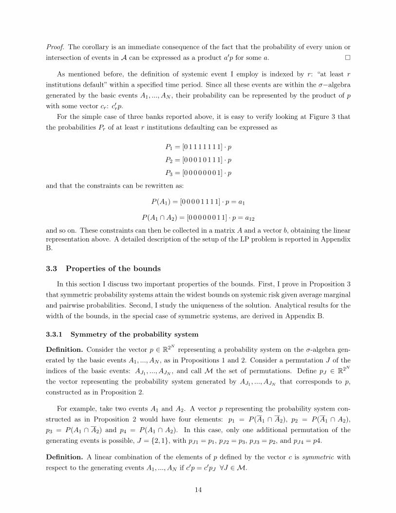
Proof. The corollary is an immediate consequence of the fact that the probability of every union orintersection of events in A can be expressed as a product a′p for some a.

As mentioned before, the definition of systemic event I employ is indexed by r: “at least rinstitutions default” within a specified time period. Since all these events are within the σ−algebragenerated by the basic events A1, ..., AN , their probability can be represented by the product of pwith some vector cr: c′rp.

For the simple case of three banks reported above, it is easy to verify looking at Figure 3 thatthe probabilities Pr of at least r institutions defaulting can be expressed as

P1 = [0 1 1 1 1 1 1 1] · p

P2 = [0 0 0 1 0 1 1 1] · p

P3 = [0 0 0 0 0 0 0 1] · p

and that the constraints can be rewritten as:

P (A1) = [0 0 0 0 1 1 1 1] · p = a1

P (A1 ∩A2) = [0 0 0 0 0 0 1 1] · p = a12

and so on. These constraints can then be collected in a matrix A and a vector b, obtaining the linearrepresentation above. A detailed description of the setup of the LP problem is reported in AppendixB.

3.3 Properties of the bounds

In this section I discuss two important properties of the bounds. First, I prove in Proposition 3that symmetric probability systems attain the widest bounds on systemic risk given average marginaland pairwise probabilities. Second, I study the uniqueness of the solution. Analytical results for thewidth of the bounds, in the special case of symmetric systems, are derived in Appendix B.

3.3.1 Symmetry of the probability system

Definition. Consider the vector p ∈ R2N representing a probability system on the σ-algebra gen-erated by the basic events A1, ..., AN , as in Propositions 1 and 2. Consider a permutation J of theindices of the basic events: AJ1 , ..., AJN , and call M the set of permutations. Define pJ ∈ R2N

the vector representing the probability system generated by AJ1 , ..., AJN that corresponds to p,constructed as in Proposition 2.

For example, take two events A1 and A2. A vector p representing the probability system con-structed as in Proposition 2 would have four elements: p1 = P (A1 ∩ A2), p2 = P (A1 ∩ A2),p3 = P (A1 ∩ A2) and p4 = P (A1 ∩ A2). In this case, only one additional permutation of thegenerating events is possible, J = 2, 1, with pJ1 = p1, pJ2 = p3, pJ3 = p2, and pJ4 = p4.

Definition. A linear combination of the elements of p defined by the vector c is symmetric withrespect to the generating events A1, ..., AN if c′p = c′pJ ∀J ∈M.

14

An example of a symmetric weighting vector c is the one corresponding to the probability of theunion of the events, c = [1 1 0 1]′, since c′p = c′pJ = P (A1 ∪A2).

Definition. A probability system p is symmetric if every event in V (the finest partition of thesample space generated by the basic events) has the same probability in all permutations of thegenerating events.

For example, with three generating events (N = 3), the probability system is symmetric ifP (A1) = P (A2) = P (A3) and P (A1 ∩A2) = P (A1 ∩A3) = P (A1 ∩A3).

Definition. A linear programming problem

max c′p

s.t. Ap ≤ b

is symmetric if c and all rows of A are symmetric with respect to the generating events A1, ..., AN .We can now state the following proposition:

Proposition 3. Suppose that the probability bounds correspond to a symmetric LP problem. Then,the bounds are attained by a symmetric probability system.

Proof. See Appendix B.

Corollary. The bounds on systemic events of the type “at least r institutions default” given a symmet-ric constraint set (for example, constraints on the average marginal and pairwise default probabilities)are attained by a symmetric probability system.

The bounds obtained in a symmetric network in which we observe all marginal and pairwiseprobabilities will always be at least as wide as those obtained in an asymmetric network with thesame averages of the low-order probabilities. The difference between the bounds obtained in thetwo cases captures precisely the extent to which asymmetry in the shape of the network affects theprobability of systemic events.

3.3.2 Uniqueness of the solution

At first sight, it might seem that if a financial network is asymmetric enough (relative to the observedmarginal and pairwise default probabilities), there will be a unique probability system that attainsthe upper bound on systemic risk, and similarly a unique one that attains the lower bound. However,this is in general not the case: several probability systems exist that attain each bound. The existenceof multiple solutions to the maximization problem plays an important role in section 5, where I studythe contribution of different institutions to systemic risk.

If more than one probability system attains the upper (lower) bound, it is possible that someprobability P (A′) of an event A′ is not completely pinned down at the bound. In this case, wecan characterize the range of possible values for this probability by solving a second maximiza-tion/minimization problem of the type:

15

maxp(minp) v′p

s.t.p ≥ 0

i′p = 1

Ap = b

c′rp = cbound

where v is the vector that corresponds to the event A′ (as described in Propositions 1 and 2),and cbound is the value of the upper or the lower bound on systemic risk. In other words, we lookfor the probability system, among those which attain the upper or the lower bound, that maximizes(minimizes) the particular probability we are interested in, P (A′). Of course, if maxpv′p = minpv

′p,that particular probability is completely pinned down at that bound on systemic risk.

In addition, we can also try to find a “representative” probability system at the upper (lower)bound. One way to construct such a system is the “AFROS” procedure described in Appa (2002)and reported in Appendix B. The “representative” probability system is obtained averaging differentprobability systems, chosen from the space of solutions to the bounds that are as distant as possiblefrom each other. In other words, then, it is an average of solutions that are as different from eachother as possible within the space of solutions to the probability bounds.

4 Implementation

The method presented in section 3 requires conditioning on marginal and pairwise default proba-bilities for all banks and all pairs of banks. When working with actual data, however, estimatingthe bounds requires some additional steps. First, in order to extract marginal and pairwise defaultprobabilities from observed prices, I need to specify a pricing model for bonds and CDSs that takesinto account not only default risk, but also other important determinants of prices - in particularliquidity premia, shown to be an important factor by several studies.20 Second, the implementationof the bounds is affected by the availability of CDS data. Because I only observe, for each bank, theaverage CDS spread quoted by its counterparties, the bounds I can estimate condition on a smallerinformation set, which captures average counterparty risk. I now discuss each of these issues in turn.

4.1 Pricing bonds

To price bonds, I use a simple pricing model of the reduced-form class with constant risk-neutralhazard rates of default, as in Lando (1997), Duffie and Singleton (1999), and Hull and White (2000,2001).

In general, four elements are crucial in determining the price of a bond: credit risk, the recoveryrate, the risk-free rate process and the liquidity premium. Assume that the recovery rate process

20For example, see Bao et al. (2010), Chen, Lesmond and Wei (2007), Collin-Dufresne, Goldstein and Martin(2007), Huang and Huang (2003), or Longstaff et al. (2005).

16

is independent of all other processes and call the expected recovery rate R. Call T the maturity ofthe bond and short term rFt the riskless rate. The reduced-form approach specifies a risk-neutraldefault hazard process ht, the risk-neutral probability of default between t and t+ 1 conditional onsurvival until t. Following Duffie (1999), I incorporate a liquidity process γt > 0. This process ismodeled as a per-period proportional cost of holding the bond. Later I discuss how we can interpretthis parameter in light on the theoretical literature on liquidity in asset markets.

I use a simplified pricing model21 that assumes that, for any given firm, the prices of all ofits bonds are determined independently at each time t, under the assumption that from time tonwards ht+s and γt+s will be constant and equal to ht and γt, respectively. Naturally, this is justan approximation, because prices do not take into account that at each future date these parametersare going to be revised, since at every future date t+r prices will be recomputed assuming a constanthazard rate and liquidity process from t+r on, at new levels ht+r and γt+r. I discretize the model toa monthly horizon, and I assume that coupons are paid monthly. The choice of a month is motivatedby the relative reference period for the CDS spreads discussed in section 2.

Theoretically it would be possible to specify and estimate more sophisticated models for hit andγit : at each time t we observe several bonds outstanding with different maturities, and thereforewe could extract information about the term structure of hit at each point t looking forward. Thereason why I choose a much simpler model as a baseline case comes from limitations in the CDSdata. Because CDS quotes obtained from the main data vendors are reliable only for the contractsof 5 year maturity, I do not have enough information to identify a corresponding term structure ofjoint hazard rates at every time t for CDSs. The assumption of constant hazard rates allows me toidentify the marginal and joint hazard rates directly combining bond and CDS spreads.22

Calling δ(t, T ) the risk-free discount rate between times t and T (the price at time t of a risk-freezero-coupon bond with maturity T ), the price at time t of a senior unsecured bond j issued by firmi, with coupon cij and recovery equal to a fraction R of the face value of the bond is:

Bij(t, T ij) = cij

T ij∑s=t+1

δ(t, s)(1− hit)s−t(1− γit)s−t+

+δ(t, T ij)(1− hit)Tij−t(1− γit)T

ij−t +R

T ij∑s=t+1

δ(t, s)(1− hit)s−t−1(1− γit)s−t−1hit

(8)

Before tackling the problem of calibrating the process γit (later in this section), it can be usefulto discuss a possible interpretation for this variable. The role of γit in the bond pricing formula is tocapture in a reduced-form way all the different elements that result in a liquidity discount in bonds,which can arise for a variety of reasons (such as funding costs, search costs and other transactioncosts, or asymmetric information). Funding costs, in particular, are an appealing motivation for

21I report the general discrete-time pricing model in Appendix C.22A way to tackle this problem under additional assumptions (essentially imposing that the term structure of joint

default follows the term structure of marginal default hazard estimated from bond prices) is explored in section 6 andAppendix D.

17

modeling the liquidity process because they are known to have been especially relevant during therecent crisis.

Garleanu and Pedersen (2010) present a model in which liquidity discounts arise because somemarket participants are required to use part of their own equity in purchasing the assets. In par-ticular, they are required to post a margin mij

t on security j of firm i at time t. Because this usesup part of their own capital, they require an additional return that is proportional to the productof mij

t and ψt, the shadow cost of funds at time t. This, in the presence of a group of traders forwhich the financing constraint is binding, leads to an adjusted CCAPM of the form:

Et[Rijt+1 −R

ft+1] = −

Covt(Mt+1, Rijt+1 −R

ft+1)

Et[Mt+1]+mij

t xtψt (9)

where Mt+1 is the CCAPM stochastic discount factor and Rijt+1 is the return on the bond, which

includes the potential liquidity discount that might arise in the future. The liquidity discount alsodepends on xt, the proportion of liquidity-constrained agents in the economy. Note that since allbonds I consider have the same seniority, we can assume that mij

t = mit for all the bonds issued by

the same firm.In the simple pricing model presented here, the term γit approximately corresponds to mij

t xtψt.23

In light of this, the liquidity component γit can be interpreted as a time-varying shadow cost of thecapital that needs to be put as margin on the bond issued by firm i. Variation of γit over timecan be attributed to changes in the margin requirements specific to firm i or to variations in theeconomy-wide weighted shadow cost of capital, xtψt.

4.2 Pricing CDSs

As explained in section 2, a potentially important component of the spread of a CDS is counterpartyrisk.24 Counterparty risk arises because in some states of the world the protection seller cannotpay the buyer the full amount owed. A fraction of that amount can still be recovered thanks tocollateralization and to the seniority of CDS claims in bankruptcy relative to junior claims.

As with bonds, I discretize the model to one month intervals, and I assume that both marginaland joint hazard rates are constant from the perspective of the time of the pricing until the maturityof the CDS (5 years). I assume that the payoff of the CDS for the following month is as follows. Ifthe seller does not default within the month but the reference entity defaults, the payment is madein full. Therefore, a month is considered an amount of time sufficient for the seller to establishwhether to default or not on the CDS obligation, given that the reference entity defaulted. If theseller defaults within the month but the reference entity does not, the contract terminates witheither a positive or a negative value (depending on whether the default probability of the referenceentity increased or decreased relative to when the contract was written). Here I assume that the

23Apart from a term Es[Ms+1]−E[Ms+1]

E[Ms+1]which captures fluctuations in the short-term risk-free rate and should be

relatively small and not very volatile.24The literature on pricing credit derivatives is very large, and examples include Das and Sundaram (2000) and Duffie

(1999). Hull and White (2001) and Jarrow and Turnbull (1995) in particular consider models of credit derivativessubject to counterparty risk.

18

expected value of the contract conditional on the reference entity surviving until the next month iszero.25

If both the seller and the reference entity default in the same month, I assume that the twodefaults happen in a connected way and only an amount S of the full payment is recovered - thiscase corresponds to the double default case, in which counterparty losses are important. The pricingformula remains approximately the same if, conditional of both firms defaulting in the same month,the default of the seller induces a jump in the order of magnitude of the probability of default ofthe other institution for a certain amount of time; as explained in section 2, double default doesnot need exact simultaneity of the defaults. Note that different assumptions about the jump inprobability when the seller defaults conditional on both banks defaulting in the same month can bemapped into different recovery rates in case of double default, S. Robustness to assumptions aboutS is explored in section 6.

Calling P (Ai) the (constant) monthly default probability of institution i, P (Ai ∩ Aj) the prob-ability of joint default during each month, and under the assumptions that these hazard rates areconstant over time and independent of the risk-free rate process, the discretized CDS pricing equationcan be written as:

T−1∑s=t

δ(t, s)(1− P (Ai ∪Aj))s−tzji = (10)

=T∑

s=t+1

δ(t, s)(1− P (Ai ∪Aj))s−t−1 [P (Ai)− P (Ai ∩Aj)] (1−R) + S [P (Ai ∩Aj)] (1−R)

where zji is the spread of the CDS written by j to insure against i’s default.The left-hand side of the formula represents the present value of payments to the protection

seller; they only occur as long as neither a credit event occurred nor the counterparty defaulted.The right-hand side represents the expected payment in case of default. In each period, conditionalon both firms surviving until then, there is a probability P (Ai) − P (Ai ∩ Aj) that the referenceentity defaults while the counterparty has not defaulted, so that the payment of (1−R) is made infull. With probability P (Ai∩Aj), there is a double-default event, and thus only a fraction S of thatpayment is recovered. Note that if only the counterparty defaults the contract ends with zero valuedue to the assumption of constant hazard rates.

Using a linear approximation derived and discussed in Appendix C, it is possible to rewrite thespread as:

zji,t = (P (Ai)− (1− S)P (Ai ∩Aj))

[∑Ts=t+1 δ(t, s)

](1−R)[∑T−1

s=t δ(t, s)] (11)

This representation is linear in the event probabilities and can then be imposed directly as a con-25This is consistent with the assumption of constant hazard rates, in which the credit risk of the reference entity

is constant over time as long as it does has not defaulted. The pricing formula remains approximately the same aslong as the hazard rate of default of the reference entity, conditional on surviving until the next month, remains ofthe same order of magnitude as it was before the default of the counterparty. In this case, the effect on the price ofthe CDS is of the order of magnitude of the square of the CDS spread, which is very small.

19

straint in the LP problem.While the model I use in this paper uses a simple discrete-time framework, it would be possible

to build continuous-time models of CDS prices that take into account the exact dynamics of eventsand the timing of defaults. Several models of joint default that appear in the literature assume thatdefaults in each (short) period ∆t are independent conditional on the realization of a state vector.In these models, counterparty risk at short horizons is very small by construction, which makesthese models less suitable to model the case in which joint default is relevant even at short horizons.A valid alternative are models of correlated default intensities, as introduced by Jarrow and Yu(2001). In these models, the default of one institution increases immediately the default intensity ofthe others. Because of limited availability of CDS pricing data, I do not have enough flexibility toestimate these models directly. However, my discrete-time pricing formulation is compatible with amodel in which defaults within a month are correlated due to spillovers from one institution to theother, but, conditional on one institution surviving until the next month, the spillover effect on thedefault intensity of other banks is small or negligible.

4.3 Implementation of the bounds: liquidity assumptions

Once the pricing models for bonds and CDSs are specified, the implementation of the boundsrequires dealing with the presence of the bond liquidity process γti , which is unobservable but acrucial determinant of bond prices. Because γti is unobservable, and because there is no unique wayof interpreting it, estimating the liquidity process directly is extremely difficult. However, it is atleast possible to obtain plausible lower bounds for it, which translate into upper bounds for themarginal probabilities P (Ai).

I start by assuming that γit can be decomposed into a fixed firm-specific component αi, anda time-varying component, λt, common to all senior unsecured bonds issued by large financialinstitutions:

γit = αiλt (12)

where λt is a latent variable normalized to be 1 on average during 2004 (the beginning of the sample),so that αi captures the average liquidity component of each bank in 2004. This formulation is flexibleenough to capture constant differences among firms in my sample, as well as changes in marginsand other liquidity-related costs that are common to the firms in the sample even though they aredifferent from the rest of the economy.

This decomposition, together with the interpretation of γit discussed above, suggests three pos-sible ways to impose a plausible lower bound on γit for the financial institutions in my sample. Thefirst approach just requires that the liquidity premium for bonds should not be negative: γit ≥ 0.

The idea behind the second approach is that we can use the early part of the sample (2004) toidentify αi, because in this period counterparty risk was considered to be essentially zero. Then,using bond prices together with CDS prices allows us to perfectly identify γit during this period: theaverage basis in 2004 pins down αi for each i. If we are willing to assume that liquidity premia wereno lower during the crisis than they were in 2004, we can impose an alternative constraint γit ≥ αi.

20

A third, more sophisticated approach tries to obtain a time-varying lower bound for the liquidityprocess, γit , by comparing the financial institutions in the sample to other non-financial institutionswith high credit ratings and therefore likely similar margins and cost of funding. A CDS written bya financial institution on a safe non-financial firm is much less likely to be affected by the risk ofdouble default. Under this assumption, I proceed as follows. For a set J of nonfinancial firms withhigh credit rating, I estimate γjt using bond yield spreads and CDS spreads together and assumingno counterparty risk. Note that assuming independence yields very similar results, since the orderof magnitude is the square of the CDS spread and therefore extremely small. I then decompose itas

γjt = αjλ∗t (13)

therefore allowing the component common to nonfinancial firms (λ∗t ) to be different from the commoncomponent of financial firms, λt. Assuming that γjt is observed with independent proportional noiseεjt , i.e. we observe:

γjt = γjt εjt (14)

we can then estimate the series λ∗t for each t using OLS (again, normalizing λ∗t to be 1 on average in2004). Since this series captures the cost of funds as well as the margin requirement of the bonds ofthese non-financial institutions (relative to the pre-crisis level), for a group J of high credit ratingnonfinancial firms it is reasonable to assume that λt ≥ λ∗t . In other words, the liquidity componentcommon to financial firms was, during the crisis, at least as high as the component common tononfinancial firms. We then obtain a third possible constraint on the liquidity process: γit ≥ αiλ∗t .

Once a lower bound γitis obtained in this way for each i, from the bond pricing equation we

immediately obtain an upper bound on P (Ai), which is the value of P (Ai) that is estimated frombond prices when γit = γi

t. This defines an upper bound function hi(γit). We can then modify the

maximization problem to find the bounds on systemic risk by replacing at each t the constraintsP (Ai) = αi with the inequality constraints (one for each i)

P (Ai)t ≤ hi(γit) (15)

This allows to preserve the LP formulation in computing the bounds. On the other hand, it willresult in wider bounds, since equalities have been replaced by inequalities.

A final caveat with the use of these liquidity assumptions is that in some periods, and forsome banks, the upper bound on the marginal default probability hi(γit) might be lower than theCDS-implied default probability (the one obtained under the assumption that counterparty riskis nonnegative). In other words, after removing the component of the yield spread attributed toliquidity, the remaining part of the yield spread can be lower than the CDS spread. For example,when the liquidity process is set so that the average basis in 2004 is zero, in 2004 half of the banks(on average) will have a positive liquidity adjusted basis. In these cases I reduce the effect of liquidityto the point where bond-implied probabilities are as high as the CDS-implied probabilities. This inturn means that the default correlation of such banks with the rest of the financial system is zero:the whole basis (in fact, even slightly more) is explained by liquidity premia, and therefore there

21

is no room for counterparty risk. This phenomenon occurs less and less frequently as the financialcrisis unfolds and the basis widens for more banks. Under the calibration of liquidity to the levelof 2004, half of the banks have a zero or positive liquidity-adjusted basis on average between 2007and Bear’s collapse, a fifth of the banks between Bear Stearns’ and Lehman’s default, and about 2banks on average after that. Under the calibration of liquidity to the basis of nonfinancials, which ishigher, we have a zero or positive liquidity-adjusted basis for two thirds of the banks between 2007and Bear, about half of the banks between Bear’s and Lehman’s collapse, and again 2 after that.

4.4 Availability of CDS data and choice of the set of intermediaries

An important factor to take into account in implementing the LP problem is the fact that I donot observe the various spreads written on a given bond i by every other institution j, but only anaverage of the quotes provided by the N − 1 counterparties:

zi =1

N − 1

∑j 6=i

zji (16)

This means that when I compute the bounds, instead of the set of constraints generated fromindividual counterparties shown in (11), I can only impose the constraint

zi =

P (Ai)− (1− S)

1

N − 1

∑i 6=j

P (Ai ∩Aj)

[∑T

s=t+1 δ(t, s)]

(1−R)[∑T−1s=t δ(t, s)

] (17)

for each i.It is important to note that this constraint assumes that the spread zi is obtained by averaging

across the spreads quoted by all other N − 1 institutions in the group considered. The CDS spreadsI use (obtained from Markit Group) are constructed as an equal-weighted average of the quotesreported by a set of dealers. Unfortunately I do not observe exactly which dealers contributedquotes at each point in time. Because of this, I consider a group of dealers that are most likely torepresent the sample from which the quotes come from. Since this market is very concentrated, andthe top 10 firms alone account for about 90% of the protection sold by volume, and for at least 2/3by trade count, including all the largest dealers according to such measures of activity should ensurethat the average spread reflects the average counterparty risk of these financial institutions. Since allof these institutions are very active in the CDS market, and therefore approximately equally likelyto contribute quotes, equal weighting seems a reasonable assumption even if not all firms contributequotes at all times.

Of course, it is possible that the spread partly reflects quotes obtained from financial institutionsoutside the group I consider, or that some of the dealers in the group do not post quotes at all times.In both cases, I would likely underestimate counterparty risk: in the former case, because quotesmay be obtained from smaller institutions for which the recovery rate of the CDS in case of doubledefault could be lower; in the latter case, because if the institutions that are not posting a quote arethe riskier ones, the average spread observed would be biased upwards. However, as long as these

22

problems affect only a few institutions at a time, the effect on the average spread should be small.To find the most active dealers during the crisis, I employ a list of the Top 15 dealers by activity

in July 2008 provided by Credit Derivatives Research. While Bear Stearns could not be a part ofthat list (it had already been bought by JP Morgan), a report by Fitch Ratings26 shows that it wasan important player in the CDS market in 2006, and therefore I include it in the sample. I dropHSBC for lack of enough bond data, so that in the end my sample includes 15 banks, 9 Americanand 6 European.27 Note that after March 15th 2008 Bear Stearns disappears, and after September12th 2008 both Lehman Brothers and Merrill Lynch drop out of the group.

The assumption of equal weighting can be relaxed, by allowing the top institutions to be over-represented in the CDS spread. In particular, because we know the ranking of the top 5 institutionsby number of contracts written for each year between 2006 and 2010, we can compute bounds inwhich these institution’s weight in the average CDS spreads is higher than the other banks. Section6 shows that results are robust to this change.

4.5 Feasible bounds

The analysis presented above allows me to reformulate the maximization problem to obtain boundson systemic risk that take into account all these factors. The optimal bounds that can be computedgiven the assumptions discussed above are as follows:

maxPr

s.t.P (Ai) ≤ hi(γi) ∀i (18)P (Ai)− (1− S)

1

N − 1

∑i 6=j

P (Ai ∩Aj)

[∑T

s=t+1 δ(t, s)]

(1−R)[∑T−1s=t δ(t, s)

] = zi ∀i (19)

which can be represented in linear form as:

maxp c′rp

s.t.p ≥ 0

i′p = 1

Cp ≤ d (20)

Ep = f (21)

where the constraint (20) corresponds to the set of constraints (18), and the constraint (21) corre-sponds to (19). These bounds can then be computed separately at each t using the cross-section ofbond and CDS prices, as well as the series for γt

i.

26Fitch Ratings, 2006, Global Credit Derivatives Survey.27The banks are: Bank of America, Bear Stearns, Citigroup, Goldman Sachs, Lehman Brothers, JP Morgan, Merrill

Lynch, Morgan Stanley, Wachovia, Abn Amro, Bnp Paribas, Barclays, Credit Suisse, Deutsche Bank, UBS. Note thatAIG does not appear because it was holding large net positions, but was not one of the main dealers in the CDSmarket by volume or trade count.

23

Note that the bond-implied constraint hi(γi) can be computed beforehand using the cross sec-tion of bonds, as explained in the next section. The bounds can then be calculated taking theupper bound on marginal probabilities, hi(γi), as given. Instead, the equations derived from CDSspreads, equations (19), do not involve a separate estimation step, and they are directly imposed asa constraint in the maximization (minimization) problem.

4.6 Data

Before turning to the presentation of the results, I present in this section some information aboutthe data used and the estimation method for the marginal default probabilities hi(γi). The datacover, with daily frequency, the period from January 2004 to June 2010.

For each of the 15 institutions considered, I obtain clean prices from Bloomberg for seniorunsecured zero and fixed coupon bonds with maturity less than 10 years.28 For TRACE-eligiblebonds, I use the closing price from TRACE as reported by Bloomberg, otherwise I look on Bloombergfor the generic closing price. I exclude callable, putable, sinkable, and structured bonds, since theirprices reflect the value of the embedded options. I remove all bonds for which I have price informationfor less than 5 trading days. I consider bonds denominated in five main currencies: USD, Euro, GBP,Yen, CHF. Since Bloomberg data on European bonds is fairly limited, I integrate it with bond pricingdata from Markit, whenever it adds at least 5 observations to the price series of each bond.

As the reference risk-free rate, I use government zero-coupon yields, obtained from Bloomberg.29

An alternative would be to use swap rates (see for example Houweling and Vorst (2005)). However,swap rates contain counterparty risk, and they are indexed to LIBOR (see Sundaresan (1991) andDuffie and Huang (1996)). Because LIBOR is the rate on unsecured loans between banks, it cannotbe considered risk-free, especially in the context of systemic risk in the financial system. Theempirical results are robust to the use of swap rates, as discussed in section 6.

Using these data, together with a calibration of the lower bound for the liquidity process γit, for

every trading day t I estimate the risk-neutral default probability hit(γit) separately for each firm,using the cross section of bonds issued by firm i which are still outstanding at time t. I employthe constant hazard rate model described above, and estimate the hazard rate using least absolutedeviations to reduce the impact of outliers. All the results are robust to the use of OLS.

Table 1 reports some statistics on the availability of bond data. In the first column, for eachinstitution, we can see the average daily number of valid bond prices available for the estimation.For example, the default probability for Bank of America hit is estimated using on average 32 bondseach day. The next columns break down this number by year. The Table shows that for someEuropean dealers, bond data is scarce especially in the early part of the sample.

Turning to CDS data, since credit default swaps are derivatives traded over the counter, they arenot always standardized. However, the 5-year CDS based on the ISDA format (which standardizes

28Given that the maturity of CDSs is 5 years, it would make sense to use outstanding bonds of remaining maturityclose to 5 years when comparing bonds and CDSs. The results are robust to other maturity brackets around 5 years- for example (2,8) and (4,6), even though this would reduce the number of institutions I can use for the estimation.

29I instead bootstrap the Swiss yield curve from the government coupon yield curve, using linear interpolation andassuming bonds trade at par.

24

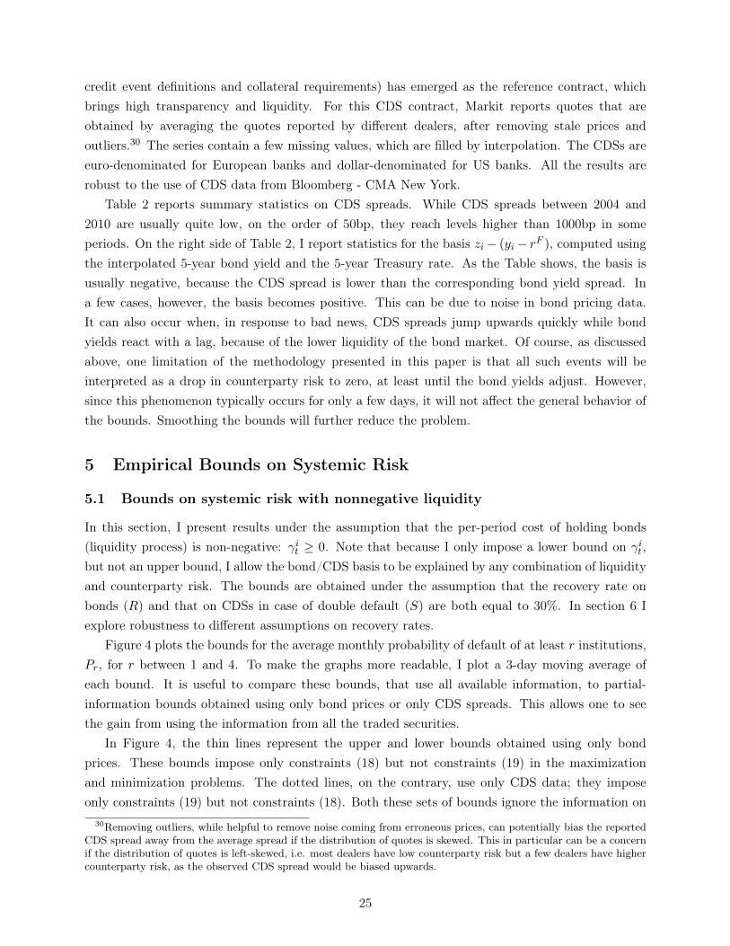
credit event definitions and collateral requirements) has emerged as the reference contract, whichbrings high transparency and liquidity. For this CDS contract, Markit reports quotes that areobtained by averaging the quotes reported by different dealers, after removing stale prices andoutliers.30 The series contain a few missing values, which are filled by interpolation. The CDSs areeuro-denominated for European banks and dollar-denominated for US banks. All the results arerobust to the use of CDS data from Bloomberg - CMA New York.

Table 2 reports summary statistics on CDS spreads. While CDS spreads between 2004 and2010 are usually quite low, on the order of 50bp, they reach levels higher than 1000bp in someperiods. On the right side of Table 2, I report statistics for the basis zi− (yi− rF ), computed usingthe interpolated 5-year bond yield and the 5-year Treasury rate. As the Table shows, the basis isusually negative, because the CDS spread is lower than the corresponding bond yield spread. Ina few cases, however, the basis becomes positive. This can be due to noise in bond pricing data.It can also occur when, in response to bad news, CDS spreads jump upwards quickly while bondyields react with a lag, because of the lower liquidity of the bond market. Of course, as discussedabove, one limitation of the methodology presented in this paper is that all such events will beinterpreted as a drop in counterparty risk to zero, at least until the bond yields adjust. However,since this phenomenon typically occurs for only a few days, it will not affect the general behavior ofthe bounds. Smoothing the bounds will further reduce the problem.

5 Empirical Bounds on Systemic Risk

5.1 Bounds on systemic risk with nonnegative liquidity

In this section, I present results under the assumption that the per-period cost of holding bonds(liquidity process) is non-negative: γit ≥ 0. Note that because I only impose a lower bound on γit ,but not an upper bound, I allow the bond/CDS basis to be explained by any combination of liquidityand counterparty risk. The bounds are obtained under the assumption that the recovery rate onbonds (R) and that on CDSs in case of double default (S) are both equal to 30%. In section 6 Iexplore robustness to different assumptions on recovery rates.

Figure 4 plots the bounds for the average monthly probability of default of at least r institutions,Pr, for r between 1 and 4. To make the graphs more readable, I plot a 3-day moving average ofeach bound. It is useful to compare these bounds, that use all available information, to partial-information bounds obtained using only bond prices or only CDS spreads. This allows one to seethe gain from using the information from all the traded securities.

In Figure 4, the thin lines represent the upper and lower bounds obtained using only bondprices. These bounds impose only constraints (18) but not constraints (19) in the maximizationand minimization problems. The dotted lines, on the contrary, use only CDS data; they imposeonly constraints (19) but not constraints (18). Both these sets of bounds ignore the information on

30Removing outliers, while helpful to remove noise coming from erroneous prices, can potentially bias the reportedCDS spread away from the average spread if the distribution of quotes is skewed. This in particular can be a concernif the distribution of quotes is left-skewed, i.e. most dealers have low counterparty risk but a few dealers have highercounterparty risk, as the observed CDS spread would be biased upwards.

25

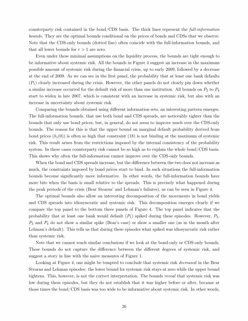
counterparty risk contained in the bond/CDS basis. The thick lines represent the full-informationbounds. They are the optimal bounds conditional on the prices of bonds and CDSs that we observe.Note that the CDS-only bounds (dotted line) often coincide with the full-information bounds, andthat all lower bounds for r > 1 are zero.

Even under these minimal assumptions on the liquidity process, the bounds are tight enough tobe informative about systemic risk. All the bounds in Figure 4 suggest an increase in the maximumpossible amount of systemic risk during the financial crisis, up to early 2009, followed by a decreaseat the end of 2009. As we can see in the first panel, the probability that at least one bank defaults(P1) clearly increased during the crisis. However, the other panels do not clearly pin down whethera similar increase occurred for the default risk of more than one institution. All bounds on P2 to P4

start to widen in late 2007, which is consistent with an increase in systemic risk, but also with anincrease in uncertainty about systemic risk.

Comparing the bounds obtained using different information sets, an interesting pattern emerges.The full-information bounds, that use both bond and CDS spreads, are noticeably tighter than thebounds that only use bond prices, but, in general, do not seem to improve much over the CDS-onlybounds. The reason for this is that the upper bound on marginal default probability derived frombond prices (hi(0)) is often so high that constraint (18) is not binding at the maximum of systemicrisk. This result arises from the restrictions imposed by the internal consistency of the probabilitysystem. In these cases counterparty risk cannot be so high as to explain the whole bond/CDS basis.This shows why often the full-information cannot improve over the CDS-only bounds.

When the bond and CDS spreads increase, but the difference between the two does not increase asmuch, the constraints imposed by bond prices start to bind. In such situations the full-informationbounds become significantly more informative. In other words, the full-information bounds havemore bite when the basis is small relative to the spreads. This is precisely what happened duringthe peak periods of the crisis (Bear Stearns’ and Lehman’s failures), as can be seen in Figure 4.

The optimal bounds also allow an interesting decomposition of the movements in bond yieldsand CDS spreads into idiosyncratic and systemic risk. This decomposition emerges clearly if wecompare the top panel to the bottom three panels of Figure 4. The top panel indicates that theprobability that at least one bank would default (P1) spiked during these episodes. However, P2,P3 and P4 do not show a similar spike (Bear’s case) or show a smaller one (as in the month afterLehman’s default). This tells us that during these episodes what spiked was idiosyncratic risk ratherthan systemic risk.

Note that we cannot reach similar conclusions if we look at the bond-only or CDS-only bounds.These bounds do not capture the difference between the different degrees of systemic risk, andsuggest a story in line with the naive measures of Figure 1.

Looking at Figure 4, one might be tempted to conclude that systemic risk decreased in the BearStearns and Lehman episodes: the lower bound for systemic risk stays at zero while the upper boundtightens. This, however, is not the correct interpretation. The bounds reveal that systemic risk waslow during these episodes, but they do not establish that it was higher before or after, because atthose times the bond/CDS basis was too wide to be informative about systemic risk. In other words,

26

a similar basis is more informative about systemic risk at times when CDS spreads and yield spreadsare high than in times when they are low.

These results were obtained under minimal assumptions on liquidity. In the next section, I showthat imposing stricter assumptions on liquidity makes the basis more informative even in the periodsbefore and after these peaks, when the levels of the spreads are lower.

5.2 Bounds with other calibrations of liquidity

As explained in section 4, if we assume that the liquidity cost of holding a bond is at least γit,

the upper bound on each of the marginal default probabilities decreases to hi(γit). In other words,the part of the bond/CDS basis that can be attributed to counterparty risk is reduced by a corre-sponding amount. In this section I show how the bounds on systemic risk vary as we make differentassumptions about γi

t. Note that lowering the upper bound on the marginal probabilities of default

has three effects on the measures of systemic risk. First, it directly rules out high values for theindividual default probabilities of each bank. Second, it indirectly lowers the maximum amountof counterparty risk present in CDS contracts, by lowering the basis for all banks. Third, to theextent that the effect of liquidity on the basis is different across dealers, it increases the asymmetryof the network and therefore leads to a greater benefit from using all the information available. Thebounds constructed using bond prices but not CDS spreads reflect only the first effect. The boundsthat use only CDS data are not affected at all by bond liquidity assumptions. The optimal boundsreflect all three effects, and therefore become significantly tighter than both the other bounds.31

The first panel of Figure 5 reports the bounds on the monthly probability of at least fourinstitutions defaulting (P4) when γi

t= 0 (which corresponds to the last panel of Figure 4). The

second panel plots bounds obtained when γitis calibrated to match the bond/CDS basis of each

bank in 2004. This calibration implies a liquidity component of the yield spread of about 50-60%in 2004 - in line with the calibrations of Huang and Huang (2003) and Longstaff, Mithal and Neis(2005).

The third panel plots the bounds obtained by calibrating the liquidity process to the one thatfits the entire basis of nonfinancial firms, as explained in section 4. In particular, I look at thenonfinancial firms that compose the CDX IG index (a standard index of CDS spreads on investment-grade bonds), restricting to those with credit rating of A1 or higher (according to Moody’s). For8 of these firms32 I have enough data to include them in the estimation of λ∗t . This time-varyingcomponent stays approximately constant until 2007, and during the crisis it increases by up to fivetimes.

Once stronger liquidity assumptions are taken into account, we discover that systemic risk was31Note that in order to calibrate the liquidity process, we use some information obtained from both bonds and

CDS spreads, because we use the bond/CDS basis in 2004 to calibrate the liquidity level αi, and because we adjustthe liquidity process so that the bond/CDS basis of each bank never becomes positive (as discussed in section 4).So the bond-only bounds and the CDS-only bounds, that use either constraints (18) or constraints (19) after suchadjustments for liquidity, will indirectly reflect some information contained in the bond/CDS basis. The bounds lookvery similar if the bond/CDS basis is used only to calibrate the liquidity process in 2004 but not used in the followingperiods.

32The eight firms are Boeing, Caterpillar, John Deere, Disney, Honeywell, IBM, Pfizer, Walmart.

27

particularly low before Bear Stearns’ collapse. In particular, the upper bound on P4 does not reflecta sharp increase in systemic risk at the beginning of 2008, contrary to the other measures of systemicrisk discussed in the introduction. The third panel in Figure 5 shows how that increase was due toidiosyncratic, not systemic risk. After jumping in March 2008, systemic risk kept increasing in arelatively smooth way up to April 2009, showing only a small spike immediately following Lehman’sdefault. The large spike that during that period we observe in CDS spreads and bond yields, reachingthe highest levels observed in the sample, corresponds to a spike in idiosyncratic default risk ratherthan in systemic default risk. This decomposition is only possible using all the information available,and is not captured when bounds are constructed using only bond prices or only CDS spreads.

The reason for this decomposition between idiosyncratic and default risk during these keyepisodes of the crisis is simple. High systemic risk in the financial sector requires low CDS spreads,relative to bond yields, for contracts written by large dealers against the default of other dealers.Since the counterparties to those contracts are in fact these same dealers, a high risk of systemicdefault ought to reduce the value of insurance contracts bought from them. However, until March2008, and again during September 2008, the bond/CDS basis was not wide enough to correspond tosuch spikes in systemic risk. This effect is evident especially when liquidity premia explicitly accountfor part of the basis.

A final remark concerns the interpretation of this decomposition in terms of objective, rather thanrisk-neutral, probabilities. We can reasonably assume marginal utility to be higher, in expectation,in systemic default events than in idiosyncratic default events. Therefore, a period in which P1 isparticularly high, but P4 is low, is likely to be due to high objective idiosyncratic default risk andlow objective systemic risk. If the large value of P1 was due to high expected marginal utility inthe corresponding idiosyncratic default events, we would expect to find P4 to be high as well, incontradiction with the empirical findings.

5.3 Full-information bounds and average-information bounds

An interesting question is to what extent one could achieve similar results on systemic risk by lookingonly at average bond and CDS spreads. As shown in section 3, bounds obtained using only averageinformation coincide with bounds obtained in a fully symmetric system. Therefore, this exercise alsoreveals the gain in terms of information about systemic risk due to the asymmetry of the financialnetwork.

The last panel of Figure 5 plots the bounds obtained under the full versus the average informationset. These are derived under the calibration of liquidity to nonfinancial firms, as in the third panel.The average information set is obtained by replacing the two sets of constraints (18) and (19) withone constraint each, obtained by averaging each of the two sets across dealers. The Figure showsthat looking at average spreads allows us to distinguish between idiosyncratic risk and systemic riskin some cases (like the weeks before Bear Stearns’ failure) but not in others (Lehman’s default). Thereason is that in the first episode the spreads and bases of most banks moved in a similar way, butin the second episode the risks were concentrated in a few banks.

28

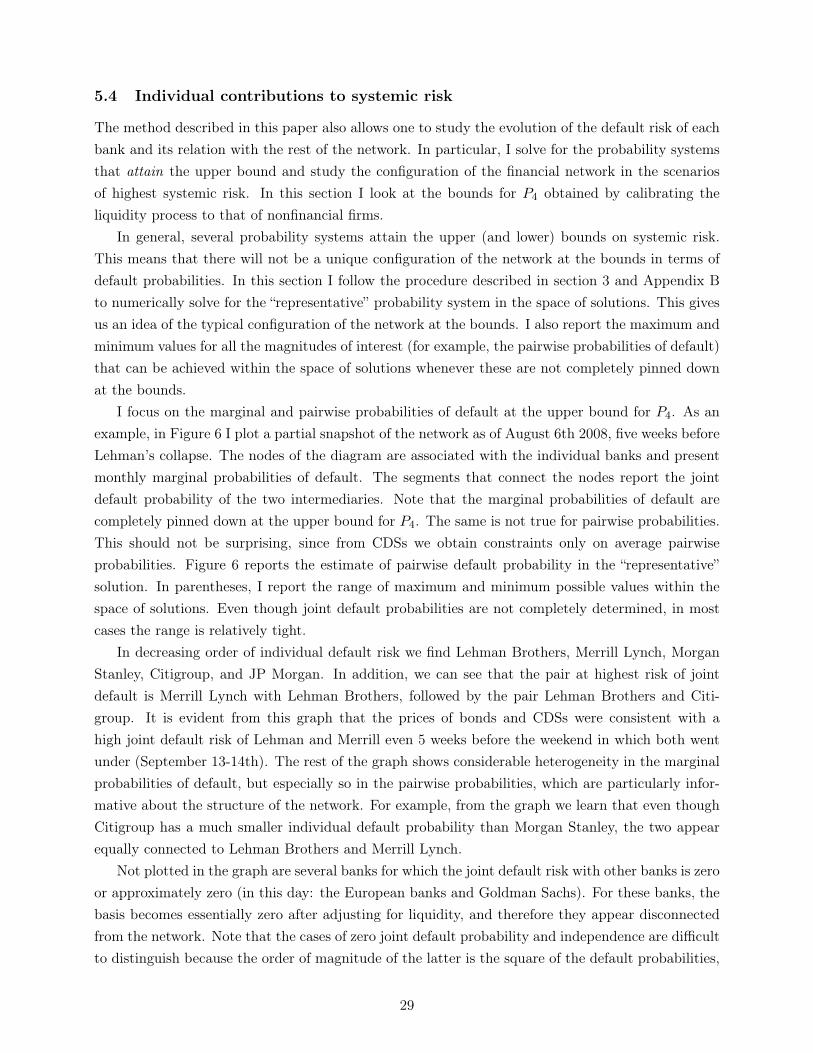
5.4 Individual contributions to systemic risk

The method described in this paper also allows one to study the evolution of the default risk of eachbank and its relation with the rest of the network. In particular, I solve for the probability systemsthat attain the upper bound and study the configuration of the financial network in the scenariosof highest systemic risk. In this section I look at the bounds for P4 obtained by calibrating theliquidity process to that of nonfinancial firms.

In general, several probability systems attain the upper (and lower) bounds on systemic risk.This means that there will not be a unique configuration of the network at the bounds in terms ofdefault probabilities. In this section I follow the procedure described in section 3 and Appendix Bto numerically solve for the “representative” probability system in the space of solutions. This givesus an idea of the typical configuration of the network at the bounds. I also report the maximum andminimum values for all the magnitudes of interest (for example, the pairwise probabilities of default)that can be achieved within the space of solutions whenever these are not completely pinned downat the bounds.

I focus on the marginal and pairwise probabilities of default at the upper bound for P4. As anexample, in Figure 6 I plot a partial snapshot of the network as of August 6th 2008, five weeks beforeLehman’s collapse. The nodes of the diagram are associated with the individual banks and presentmonthly marginal probabilities of default. The segments that connect the nodes report the jointdefault probability of the two intermediaries. Note that the marginal probabilities of default arecompletely pinned down at the upper bound for P4. The same is not true for pairwise probabilities.This should not be surprising, since from CDSs we obtain constraints only on average pairwiseprobabilities. Figure 6 reports the estimate of pairwise default probability in the “representative”solution. In parentheses, I report the range of maximum and minimum possible values within thespace of solutions. Even though joint default probabilities are not completely determined, in mostcases the range is relatively tight.

In decreasing order of individual default risk we find Lehman Brothers, Merrill Lynch, MorganStanley, Citigroup, and JP Morgan. In addition, we can see that the pair at highest risk of jointdefault is Merrill Lynch with Lehman Brothers, followed by the pair Lehman Brothers and Citi-group. It is evident from this graph that the prices of bonds and CDSs were consistent with ahigh joint default risk of Lehman and Merrill even 5 weeks before the weekend in which both wentunder (September 13-14th). The rest of the graph shows considerable heterogeneity in the marginalprobabilities of default, but especially so in the pairwise probabilities, which are particularly infor-mative about the structure of the network. For example, from the graph we learn that even thoughCitigroup has a much smaller individual default probability than Morgan Stanley, the two appearequally connected to Lehman Brothers and Merrill Lynch.

Not plotted in the graph are several banks for which the joint default risk with other banks is zeroor approximately zero (in this day: the European banks and Goldman Sachs). For these banks, thebasis becomes essentially zero after adjusting for liquidity, and therefore they appear disconnectedfrom the network. Note that the cases of zero joint default probability and independence are difficultto distinguish because the order of magnitude of the latter is the square of the default probabilities,

29

which is extremely small. However, this clearly indicates that there is ample heterogeneity acrossbanks in their maximum possible contribution to systemic risk.

Using a similar approach, for each pair of banks i and j we can track the evolution of P (Ai), P (Aj)

and P (Ai ∩ Aj) over time. Figure 7 plots a 3 day moving average of these probabilities for threedifferent pairs (all combinations of Lehman, Merrill Lynch, and Citigroup) - in the “representative”solution. The upper panel reports the marginal probabilities, and the lower panel reports the jointprobabilities. These graphs confirm the relatively high degree of heterogeneity and variability inmarginal default probabilities across banks, but even more so for joint probabilities. It is particularlyinteresting to note that the markets anticipated the joint collapse of Lehman Brothers and MerrillLynch for the two months prior to that event.

We can now turn to study how each institution contributed to systemic risk. One way to capturethis is to compute the probability that institution i is involved in a multiple default event:

Prat least 4 default ∩ i defaults

By applying the techniques described in section 3, we can verify that this probability is uniquelyidentified at the upper bound on systemic risk. Figure 8 plots this contribution for four banks(Citigroup, Lehman Brothers, Merrill Lynch and Bank of America) as well as the average across theother banks.33

As the Figure shows, there is large heterogeneity across dealers, both in the levels and in thechanges. While the contribution to systemic risk increases for all banks after August 2007, the growthis faster for Lehman and Merrill Lynch than for the other banks. Markets seem to have anticipatedthe increased systemic importance of these two institutions before the weekend of September 15th.After September 2008, Citigroup displayed the largest spike, followed immediately by Bank of Amer-ica, that ended with the release of the results of the U.S. government stress test on banks’ capitalin May 2009.

6 Robustness

In this section I study the robustness of the main results of the paper to different assumptions. Whilethe main results are easy to read in graphs like Figures 4 and 5, for reasons of space I cannot reportall the graphs for each robustness test. Instead, I report the average value of the bounds for differentsubperiods, chosen to reflect the main events identified in the Figures. For each robustness test (allperformed under the calibration of the liquidity to the basis of nonfinancial institutions, γi

t= αi

tλ∗t ) I

report in Table 3 the average value of the bounds, in basis points per month, during different periods:January to December 2007, January 2008 to March 15 2008 (the run-up to Bear Stearns’ collapse),from Bear’s episode to Lehman’s default (on September 15th 2008), the month after Lehman’sdefault (in which CDS spreads and bond yields spiked), the period between September 2008 andApril 2009 (the latest peak of the crisis, just before the stress test results were released) and finally

33To improve readability, I plot a two week moving average.

30

from May 2009 to June 2010. In the three panels, I show values for the lower and upper bound onP1, and the upper bound on P4 (the lower bound on P4 is always 0).

Besides showing the level and the time series of the bounds, this Table allows us to check thatthe main results reported in the paper hold under different assumptions. The bold line in each panelof Table 3 reports the baseline case presented in the paper. We can confirm the result, presented inFigure 5 (third panel), that systemic risk was low in the months preceding Bear Stearns’ collapse,while idiosyncratic risk was already high. Besides, we can see that during the month after Lehman’sdefault, idiosyncratic risk spiked (it increased sharply and then decreased as sharply). The upperbound on P4 increases as well, but does not even reach the level observed in the following 6 months:systemic risk keeps increasing until March 2009.

6.1 Pricing assumptions

6.1.1 Value of the constant expected recovery rates

Let us start with robustness with respect to the assumed recovery rate of CDSs when double defaultoccurs, S ∈ [R, 1]. The effect of changes in this assumption depends crucially on the liquidity-adjusted bond/CDS basis of each bank. For some banks, the basis is small enough that can becompletely explained by counterparty risk. For these banks, an increase in S means that the samebasis can account for higher counterparty risk. For other banks, instead, the basis is large enoughthat, due to internal constraints of the probability system, it cannot be completely explained bycounterparty risk: even at the upper bound for systemic risk, a part of the basis must be explainedby liquidity. For these banks, an increase in S means that the same amount of counterparty risk- which was already at the maximum possible - will explain an even smaller fraction of the basis.This means that the marginal probability of default, P (Ai), has to decrease. In turn, this directlyreduces the maximum possible amount of counterparty risk for contracts written by i against otherbanks, since for each j we must have P (Ai ∩Aj) ≤ P (Ai).

An increase in S then has a different effect on banks with a relatively small basis and banks witha large basis. The two effects are also at play for each bank individually, for different starting levelsof S: when S is low enough counterparty risk has a large effect on CDS spreads, and therefore thebasis will be relatively small - it can be completely explained by counterparty risk. When S is largeenough, not all basis can be explained by counterparty risk, and the second mechanism operates.In Appendix B, I show these results formally in the symmetric case, where all banks have the samebasis. In the asymmetric case, the two opposite forces counterbalance each other in such a waythat the bounds on systemic risk are not very sensitive to assumptions on S. The reason is that inan asymmetric network different banks will have different bases, so that for most values of S thetwo effects described above will operate for some banks in one direction and for other banks in theopposite direction. This analysis explains why we see the bounds on systemic risk being very robustto changes in S (at least up to a recovery rate of 90%), as shown in Table 3.

The case for the recovery rate of bonds R is different. As shown in equations (8) and (11), Raffects the prices of both bonds and CDSs. A higher expected recovery rate in case of default increasesthe value of a bond, and at the same time decreases the value of CDS insurance written on that

31

bond, since the payment from the CDS seller covers only the amount of bond value not recoveredin default. Because this recovery rate multiplies the marginal and joint default probabilities in thepricing formulas, when R changes all probabilities implied in bonds and CDSs are scaled up or downby approximately the same amount.34 Therefore, the bounds on systemic risk will scale in a similarway. However, the main results on the time series of the bounds will not change, as shown by Table3.

6.1.2 Time varying recovery rates

Above I have studied robustness to different assumptions about S and R, when these are assumed tobe constant during the whole sample period. In theory, it is possible that these recovery rates varyover time in a way that affects the results on the time-series of systemic risk presented in section 5.Suppose that at every time t bonds and CDSs are still priced assuming that at all future periodst+ s the recovery rates are constant and equal to St and Rt; however, let now St and Rt vary overtime. How will this affect the bounds on systemic risk?

The tests presented above show that the bounds on systemic risk scale in the same direction asR. If we believe that, during peak episodes like the one following Lehman’s default, recovery ratesR might have dropped, this would in fact strengthen the result that the spike in systemic risk wasthen relatively low, because it would further reduce the bound on P4 during that month.

Another possibility is a reduction in the recovery rate of CDSs, S, in times when systemic riskincreases. However, it is easy to see that this case actually reinforces the main empirical results. Ifthe recovery rate S becomes smaller during the key episodes of the crisis, then joint default risk hasto be smaller as well. This stems once more from the fact that during these episodes the bond/CDSbasis is small relative to CDS and yield spreads. When S is reduced, the probability of joint defaulthas a greater effect on the basis. To still match the basis even if S is higher, joint default risk has todecrease. Therefore, the main results in the paper will be robust to a decrease in the recovery rateS in times of crisis.

6.1.3 Stochastic recovery rate on bonds R

Another possibility is that when pricing bonds and CDSs, agents incorporate the possibility thatrecovery rates might be stochastic and correlated with the default events in the financial sector. Inparticular, one could think that recovery rates of both bonds and CDSs might deteriorate the moredefaults happen in the financial system.

Because of the limited data available, it is difficult to solve explicitly for the case of stochasticrecovery rates. However, it is possible to gain some intuition on the effect of this assumption undersimple modeling assumptions. Suppose that the recovery rate on bonds is RH whenever one bankdefaults alone, and RL < RH whenever two or more banks default. Then, I show in Appendix Dthat we can decompose as follows the change in the bounds on systemic risk, going from a non-stochastic recovery rate R to the stochastic recovery process described above. First, we can shift

34The difference between the two comes from differences in the cash flow timing of bonds and CDSs. They arescaled by exactly the same amount in the simple two-period example of section 2.

32

the (constant) recovery rate downwards for both bonds and CDSs to RL. This component scalesdown the bond-implied and the CDS-implied probabilities by a similar amount, as discussed above.This would scale the bounds on systemic risk downwards. Second, we increase the present valueof bonds by an amount Ybond, and decrease the present value of payments of the CDS contract byan amount YCDS ≈ Ybond (in a first-order approximation with small probabilities of default). Thissecond effect shifts the CDS spread and the yield spread in the same direction by a similar amount,with minimal effect on the basis and hence on counterparty risk. We then expect the bounds onsystemic risk to become lower if we introduce a stochastic recovery rate with RL < R. The reason isthat for the purpose of systemic risk, the relevant recovery rate is the one that obtains in states ofmultiple defaults, or RL in this case. However, as long as the recovery rates RL and RH themselvesdo not vary over time, the time series of the bounds should still look as in Figures 4 and 5.

6.1.4 Assumptions about the hazard rate

In this section I allow for a more flexible form for the hazard rate process. In particular, for eachinstitution i, from the perspective of an agent pricing bonds at time t, the hazard rate at time t+ s

follows the (deterministic but time-varying) process

ht+s = (1− ρt)ht + ρtht+s−1 (22)

where parameters ht, ht and ρt are determined at time t. As before, all bonds are priced at everytime t assuming that the hazard rate process is known for all future dates.

At each time t, I can use bond prices to estimate ht, ρt and ht. This representation allows tocapture cases in which the hazard rate is higher at shorter horizons and then reverts to a lowerlong-term value. I can therefore construct the bounds on systemic risk using ht, the probability ofdefault in the month after t.

As discussed in section 4, the main problem with this approach is that while it is easy to estimatea more flexible function for the marginal hazard rate of default using bond prices, CDS data do notcontain enough information to estimate a similarly flexible process for joint default risk (becauseat each time t we only observe the spread of one CDS, with maturity of 5 years). To tackle thislimitation, I assume that the joint hazard process replicates the shape of the marginal hazard processof the reference entity: the process decays at the same rate (ρt) and displays the same ratio betweenshort-term and long-term default hazards (ht/ht). The details of the estimation method and of theadditional assumptions involved are reported in Appendix D. Table 3 shows that the main empiricalresults are confirmed under these assumptions.

6.2 Other robustness tests

6.2.1 Using interest rate swaps as the risk-free rate

While swap rates may not be the appropriate rate to discount cash flows under risk neutral probabil-ities (because they are indexed to a risky reference, LIBOR, and because they contain counterparty

33

risk), it is interesting to check how the results change if we use them in place of Treasury rates.35

Because these rates are higher than the Treasury rates, and therefore result in a lower basis for allbanks, we would expect the upper bounds on systemic risk to decrease noticeably. At the sametime, remember that we are calibrating the time variation in the liquidity process to the basis ofnon-financial firms, and the level of the liquidity process to the basis of each bank in 2004. Therefore,the change in the risk-free rate will be offset by a corresponding decrease in the liquidity process(even though the offset is not exactly one to one). Table 3 shows that the change in the bounds isvery small.

6.2.2 Assumptions about the weighting of contributors in CDS contracts

As discussed in section 4, the bounds are computed under the assumption that the CDS spreadsare obtained by averaging quotes obtained from all the other dealers in the sample. If some dealersdo not post quotes at all times, the average spread observed will, in expectation, overweight dealerswhich send quotes in more frequently. In turn, this is most likely related to how active the dealer isin the CDS market.

While we cannot obtain directly estimates of the activity of the dealers (in terms of numberof contracts written and volume of CDS protection sold), Fitch Ratings36 reports a ranking of thetop 5 counterparties by trade count (which in turn is very correlated with gross positions sold), foreach year between 2006 and 2010. We might then think that because these dealers are more active,quotes are more likely to be obtained from them, and therefore the average CDS spread observedwill in expectation reflect more their contribution. Given this, as a robustness test I compute boundsthat overweight the top 5 institutions in the formula for CDS contracts. I consider two relativelyextreme weighting schemes. In all of them, institutions ranked below 5 have the same weight (I donot have information about the relative ranking of these dealers). In the first weighting scheme, Icompute the bounds assuming that the top 5 institutions are 5 times more likely than the other10 to contribute quotes, and therefore their contribution is weighted 5 times more than the otherinstitutions in the sample. The second weighting scheme again assumes that all institutions ranked6-15 have the same weight, and the top dealer has 10 times their weight, the second dealer 8 times,and so on up to the 5th largest dealer (with a weight twice that of the smaller dealers).

The effect of this overweighting on the bounds of systemic risk is not immediate. Suppose, forexample, that in the bounds computed under equal weighting, systemic risk comes from the jointdefault risk among top-5 banks. Then, increasing the weight on these banks will have the effect,everything else constant, of lowering the weighted CDS spreads. But this is not possible because theCDS spreads were chosen to match the observed ones. Therefore, the joint default risk among thesebanks will have to decrease. At the same time, joint default risk with smaller banks can increase.But if these smaller banks were contributing little to default risk before the change in weights, anincrease in the possibility of joint default risk with them might not make up for the reduction in

35I bootstrap the zero-coupon yield curve from the par swap rate curve of the different currencies using linearinterpolation.

36Fitch Ratings, 2008, Global Credit Derivatives Survey.

34

maximum systemic risk coming from the top-5 dealers. In this example, systemic risk will likelydecrease when we overweight top-5 dealers. It is easy to see that the opposite is true if systemic riskmainly comes from non top-5 dealers.

If instead in both groups (top-5 and non-top-5 dealers) we find dealers with large contribution tosystemic risk as well as dealers with small contribution to systemic risk, under equal weighting, thebounds will be relatively robust to changes in the weights. In fact, this is the case. The top 5 banksinclude both banks with high contribution to systemic risk as well as banks with low contributionto systemic risk, such as one or two European banks. Table 3 shows that under both weightingschemes the main results still hold.

6.2.3 Assumptions about the exchange rate

The construction of the bounds on systemic risk involves the estimation of risk-neutral probabilitiesfrom bond prices and of joint default probabilities from CDS spreads. Using probabilities obtainedfrom different securities to obtain risk-neutral probabilities of joint default requires additional as-sumptions if the securities are denominated in different currencies. In particular, while most bondsissued by American firms and the CDSs written on them are denominated in dollars, European firmsissue several bonds in Euros and in other currencies, and the CDSs written on them are denominatedin Euros.

To simplify the discussion, consider one-period bonds and CDSs written by banks i and j. Callmse the stochastic discount factor of a US investor in state (s, e). Here, s indicates the default stateof the banks i and j, so that it can take values i (only i defaults), j (only j defaults), ij (bothdefault), and 0 (none defaults). e indicates the exchange rate with a foreign currency. Call πs theprobability of s occurring, and note that πsE[mse|s] is the price of a security that pays 1 if defaultstate s happens. The price of a state-contingent security that pays a unit of foreign currency ifdefault state s happens is then πsE[emse|s].

Appendix D shows that a sufficient condition for correctly estimating risk-neutral default proba-bilities using bonds and CDSs denominated in different currencies (using the risk-free rates denom-inated in the respective currencies to discount cash flows) is:

πsE[e ·mse|s]πsE[mse|s]

=E[e ·mse]

E[mse](23)

which requires that the relative price of domestic and foreign risk-free securities is the same as therelative price of domestic and foreign state-contingent securities that pay off in the various defaultstates. Of course, it is reasonable to assume that the relative price of dollar-denominated and foreigncurrency-denominated default-contingent securities might be different depending on the default state(think for example of a flight-to-quality to US securities if several banks default). As a robustnesstest for the validity of the bounds in case these conditions are violated, I perform the estimationexercise including only American firms, for which all bonds and CDSs are dollar-denominated. Table3 shows that the results still hold for this subset of banks.

35

6.2.4 Using only larger transactions from TRACE

A concern with using bond prices from Bloomberg is that they might incorporate stale information(for European bonds, for which I use quoted prices), or they might depend on very small trades,which might be less reflective of credit risk (see for example Dick-Nielsen et al. (2010)). To makesure results are robust to these problems, I compute the bounds for the subset of US firms using onlytransaction data from TRACE, and ignoring all trades with nominal amounts of less than $100,000.Of course, this will exclude several bonds for several days. Table 3 reports that the bounds changevery little.

7 Conclusion

This paper shows that bond prices and CDS spreads represent a rich information set for learningabout joint default probabilities of intermediaries in the financial network. This information setcan be used to construct bounds on the probability of systemic events, defined as the probabilityof several institutions defaulting within a short time horizon. These bounds are the best possibleones given the available information, and they are obtained as the solution to a linear programmingproblem.

Even under minimal assumptions on the liquidity premia in bond markets, the bounds obtainedin the paper are significantly tighter than the ones obtained from bond prices alone. They are alsotighter than bounds that only use CDS spreads, particularly when CDS and bond spreads increasewhile the bond/CDS basis remains relatively small (such as early 2008 and October 2008). Addingrelatively mild assumptions on the bond liquidity process further tightens the bounds. Using thismethodology to estimate stress in the financial network helps us to better understand the recentfinancial crisis. Systemic risk started to increase in August 2007 but remained relatively low untilafter Bear Stearns’ collapse. After that, the bounds widen considerably, which would be consistentboth with an increase in systemic risk and with an increase in uncertainty about the severity of suchrisks. Finally, the bounds on systemic risk converge to lower values starting in the second half of2009.

This paper shows how it is possible to decompose the changes in bond and CDS spreads across thenetwork into an idiosyncratic and a systemic component of default risk. By using the full informationset available from observed prices, the bounds show that some of the spikes in bonds yields and CDSspreads of financial institutions during the crisis correspond to increases in idiosyncratic defaultrisk rather than systemic risk. This is the case for the months preceding March 15th 2008 (BearStearns episode) and following Lehman’s default. This decomposition is important to understandthe market’s perceptions of risk during the financial crisis.

The same methodology can also be used to track the contribution to systemic risk of the insti-tutions comprising the financial network, as well as to obtain a full representation of the defaultprobabilities in the financial network in the scenario of highest systemic risk. An interesting resultthat emerges from this analysis is that markets seem to have anticipated the possible systemic na-ture of the risk exposure of some banks (Lehman and Merrill Lynch), several weeks before these

36

institutions faced a severe crisis in September 2008: the upper bound on the joint default probabilityand the contributions to systemic risk of these two banks increased dramatically already by July2008.

It is worth noting some limitations of the approach. The bounds capture market perceptionsabout probabilities rather than the true probabilities. This means that just as securities can bemispriced, the bounds can reflect various imperfections and mispricing that happen in financialmarkets, including slow incorporation of information and underestimation of risks. In addition,because they are reduced-form, they do not allow us to distinguish whether the low systemic riskestimated, for example, around March 2008 was due to the configuration of structural links betweenthe banks or because of the expectation of government intervention in case multiple banks defaulted(which is what happened in September 2008). This also limits their use for policy action. Bond,Goldstein and Prescott (2010) warn us of the danger of taking actions based on market priceswhen these prices incorporate anticipation of the policy response. On the other hand, the boundsrule out some of the accounts about perceived risks, such as the fear of the government leavingseveral banks to default in the case that shocks propagated throughout the system. Also, whilethe approach is built to minimize the number of assumptions about the correlation structure of thenetwork, especially regarding high-order joint risks, some assumptions are still necessary to obtainthe bounds. For example, estimating risk-neutral marginal and pairwise default probabilities fromprices requires imposing a pricing model and taking a stand on the effects of liquidity in bondmarkets.

The method developed in this paper can easily be extended to incorporate information fromadditional securities. The price of any security whose payoff depends on individual or joint defaultscan be added as a constraint in the maximization and minimization problems, thus tightening thebounds. For example, the prices of CDS baskets and equity index options may enrich the informationset and improve the measurement of systemic risk. In the future, as better data on these and othersimilar securities become more easily available, the measurement of systemic risk will become evenmore precise.

Because this method allows us to measure not only the aggregate level of systemic risk, but alsothe linkages between institutions, it opens the way to new studies of the structure of the financialsystem. For example, one can explore which network structures are more robust to financial distress,or the effect of individual banks’ decisions on the aggregate level of systemic risk.

Since the bounds presented in this paper can be constructed in real time, they can be used tocomplement other measures in monitoring the market’s perceptions of systemic risk. Not only dothey track the effect of macroeconomic and financial shocks on perceived systemic risk, but they alsoreflect the market’s expectations regarding government intervention in financial markets. Finally,the possibility of measuring in real time the structure of the financial network can be a valuable toolfor identifying the sources of distress among banks at the core of the financial system.

37

References

Acharya, Viral V., Lasse H. Pedersen, Thomas Philippon and Matthew Richardson, 2010, “Measur-ing systemic risk”, NYU Working Paper.

Adrian, Tobias and Markus K. Brunnermeier, 2009, “CoVaR,” Staff Reports 348, Federal ReserveBank of New York.

Anderson, Ron, 2009, “What Accounts for Time Variation in the Price of Default Risk?”, LSEWorking Paper.

Appa, Gautam, 2002, “On the uniqueness of solutions to linear programs”, Journal of the OperationalResearch Society, 53, no. 10, 1127-1132.

Arora, Navneet, Priyank Gandhi and Francis Longstaff, 2009, “Counterparty Credit Risk and theCredit Default Swap Market”, UCLA Working Paper.

Avesani, Renzo, Antonio Pascual and Jing Li, 2006, “A New Risk Indicator and Stress Testing Tool:A Multifactor Nth-to-Default CDS Basket,” IMF Working Papers 06/105.

Bao, Jack, Jun Pan and Jiang Wang, 2008, “Liquidity of Corporate Bonds”, MIT Sloan WorkingPaper.

Barro, Robert, 2006, “Credit-Default Swaps and Default Probabilities”, unpublished, Harvard Uni-versity.

Berndt, Antje, Robert Jarrow, and ChoongOh Kang, 2007, “Restructuring Risk in credit defaultswaps: An empirical analysis”, Stochastic Processes and their applications, Vol 117 n. 11.

Blanco, Roberto, Simon Brennan, and Ian W. Marsh, 2003, An empirical analysis of the dynamicrelationship between investment grade bonds and credit default swaps, The Journal of Finance,Vol. 60, No. 5 (Oct., 2005), pp. 2255-2281.

Bond, Philip, Itay Goldstein and Ed Prescott, 2010, “Market-Based Corrective Actions”, Review ofFinancial Studies 23, 781-820.

Boros, E. and A. Prékopa, 1989, “Closed Form Two-Sided Bounds for Probabilities that at Least rand Exactly r out of n Events Occur”, Mathematics of Operations Research 14, 317-342.

Chen, Long, David Lesmond and Jason Wei, 2007, “Corporate Yield Spreads and Bond Liquidity”,Journal of Finance 42, 119-149.

Cihak, Martin and Klaus Shaeck, 2007, “How Well Do Aggregate Bank Ratios Identify BankingProblems?”, IMF Working Paper 07/275.

Collin-Dufresne, Pierre, Robert S. Goldstein, and J. Spencer Martin, 2001, “The determinants ofcredit spread changes”, Journal of Finance 56, 2177–2207.

Das, Sanjiv R., and Rangarajan K. Sundaram, 2000, “A discrete-time approach to arbitrage-freepricing of credit derivatives”, Management Science 46, 46–62.

38

Demirguc, Asli and Enrica Detragiache, 1998, “The Determinants of Banking Crises in Developingand Developed Countries”, IMF Staff Paper 45/1.

Demirguc, Asli and Enrica Detragiache, 1999, “Monitoring Banking Sector Fragility: A MultivariateLogit Approach”, IMF Working Paper 99/147.

De Wit, Jan, 2006, “Exploring the CDS-bond basis”, National Bank of Belgium Working Paper.

Dick-Nielsen, Jens, Peter Feldhuetter, and David Lando, 2010, “Corporate bond liquidity before andafter the onset of the subprime crisis”, Working Paper.

Duffie, Darrell, 1999, “Credit swap valuation”, Financial Analysts Journal 55, 73–87.

Duffie, Darrell, and Ming Huang, 1996, “Swap rates and credit quality”, Journal of Finance 51,921-949.

Duffie, Darrell, and Kenneth J. Singleton, 1999, “Modeling term structures of defaultable bonds”,Review of Financial Studies 12, 687–720.

Duffie, Darrell, and Haoxiang Zhu, “Does a Central Clearing Counterparty Reduce CounterpartyRisk?”, Stanford GSB Research Paper.

Garleanu, Nicolae G. and Lasse H. Pedersen, 2010, “Margin-Based Asset Pricing and Deviationsfrom the Law of One Price”, NYU Working Paper.

Gonzales-Hermosillo, Brenda, 1999, “Determinants of ex-ante Banking System Distress: A Macro-Micro Empirical Exploration of Some Recent Episodes”, IMF Working Paper 99/23.

Houweling, Patrick, and Ton Vorst, 2004, “Pricing default swaps: Empirical evidence”, Journal ofInternational Money and Finance, 29 1331–1358.

Huang, Jing-zhi, and Ming Huang, 2003, “How much of the corporate-Treasury yield spread is dueto credit risk?”, Working paper, Penn State University.

Huang, Xin, Hao Zhou, and Haibin Zhu, 2009, “A Framework for Assessing the Systemic Risk ofMajor Financial Institutions”, Journal of Banking and Finance, vol 33 no. 11.

Hull, John C., and Alan D. White, 2000, “Valuing credit default swaps I: No counterparty defaultrisk”, The Journal of Derivatives 8, 29–40.

Hull, John C., and Alan D. White, 2001, “Valuing credit default swaps II: Modeling default corre-lations”, The Journal of Derivatives 8, 12–22.

Jarrow, Robert A., and Stuart M. Turnbull, 1995, “Pricing derivatives on financial securities subjectto credit risk”, Journal of Finance 50, 53–85.

Jarrow, Robert A., and Fan Yu, 2001, “Counterparty risk and the pricing of defaultable securities”,Journal of Finance 56, 1765-1799.

Kritzman, Mark, Yuanzhen Li, Sebastien Page and Roberto Rigobon, 2010, “Principal Componentsas a Measure of Systemic Risk”, Revere Street Working Paper 272-28.

39

Kwerel, S.M., 1975, “Most stringent bounds on aggregated probabilities of partially specified depen-dent probability systems,” Journal of the American Statistics Association 70, 472-479.

Lando, David, 1997, “Modelling bonds and derivatives with credit risk”, in M. Dempster and S.Pliska (eds.), Mathematics of Financial Derivatives, pp. 369–393, Cambridge University Press.

Lehar, Alfred, 2005, “Measuring systemic risk: A risk management approach”, Journal of Bankingand Finance, vol. 29 no. 10.

Longstaff, Francis, Sanjay Mithal and Eric Neis, 2005, “Corporate Yield Spreads: Default Risk orLiquidity? New Evidence from the Credit-Default Swap Market”, Journal of Finance, Vol. 60,No. 5.

Merton, Robert C., 1974, “On the Pricing of Corporate Debt: The Risk Structure of Interest Rates”,Journal of Finance, Vol. 29, No. 2.

Poghoshan, Tigran and Martin Cihak, 2009, “Distress in European Banks: An Analysis Based on aNew Data Set”, IMF Working Paper 09/09.

Segoviano, Miguel, 2008, “The CIMDO Copula. Modeling of a Non-Parametric Copula”, IMFWorking Paper

Segoviano, Miguel and Charles Goodhart, 2009. "Banking Stability Measures," IMFWorking Papers09/4, International Monetary Fund.

Singh, Manmohan and James Aitken, 2009, “Counterparty Risk, Impact on Collateral Flows, andRole for Central Counterparties”, IMF working paper 09/173.

Singh, Manmohan, 2010, “Collateral, Netting and Systemic Risk in the OTC Derivatives Market”,IMF working paper 10/99.

Sundaresan, S. ,1991, "Valuation of Swaps.", in Recent Developments in International Banking andFinance, S. Khoury, ed. Amsterdam: North Holland (Vols. IV and V, 1991).

40

Appendix

Appendix A - Collateral agreements and the pricing of counterparty risk

In the text, I argue that the collateral agreements used for CDS contracts during the financial crisis wereunlikely to eliminate counterparty risk. Buyers of CDS protection were aware of this and possibly priced itinto the spreads. Here I report some evidence for the main points of the argument.

An initial question is whether counterparty risk was perceived at all by market participants. The growthof the percentage of OTC derivative contracts covered by some form of collateral confirms this indirectly:for credit derivatives, the volume-weighted percentage of collateralized contracts went from 39% in 2004 to58% in 2005, to 66% in 2007 and 2008 (ISDA Margin Survey 2006, 2008). Besides, documents and interviewsfrom practitioners directly confirm that the issue was taken into account by financial participants throughoutthe crisis. Robert McWilliam, head of Counterparty Risk management at ABN Amro, reports in January200837: “The golden rule is to start early. If you start worrying about the counterparty when they are underduress your options are fairly limited”. A document from Barclays dated February 200838 states:“While themaximum potential loss to the seller of protection is the contract spread for the rest of the contract duration,the buyer of protection could arguably lose the full notional of the contract (in case of simultaneous defaultsby counterparty and the reference credit and zero recovery). Thus, counterparty risk is evidently more of aconcern for buyers of protection.”

Even if agents were aware of counterparty risk, it was standard practice to ask for relatively little collateral,especially from the largest counterparties. ISDA reports that only about 2/3 of the contracts were covered bya collateral agreement, up to 2009. Besides, calculations by Singh and Aitken (2009) and Singh (2010) showthat, even at the end of 2009, large financial institutions still carried large under-collateralized derivativeliabilities. In particular, they compute the total value of “residual derivative payables” - liabilities fromderivative positions after netting under master netting agreements and in excess of the collateral posted.For the 5 largest US dealers this amount was more than $250bn. Even though these numbers include allderivative contracts, and not only CDSs, they suggest a general under-collateralization of derivative positionsfrom these counterparties. As an example of this, in 2008 Goldman Sachs had received collateral for 45%of the value of its receivable OTC derivatives, but posted only 18% of the value of payables. Similarly, JPMorgan in the same year had received collateral for 47% of receivables, but posted only 37% of the payables39.Finally, as reported in the main text, even the most active dealer in counterparty risk management, GoldmanSachs, failed to cover the full value of exposure on its CDS position with AIG.

Even when a collateral agreement is in place and actively managed, residual counterparty risk cannot beeliminated when the value of the derivative is subject to jumps. While during the crisis we did see gradualincreases in CDS spreads of banks, a crucial episode - the Lehman bankruptcy - shows that correlated jumpsin credit risk (and defaults) are indeed possible. Just before the weekend of the 13th and 14th of September2008, many institutions were considered at risk, but neither the credit ratings nor the CDS spreads indicatedan extremely high likelihood of immediate default. For example, the Lehman 5 year CDS was trading ataround 700bp per year, Merrill’s at 400bp, and the credit ratings of their debt were still as high as 4 monthsbefore, with an implied default probability of less than 0.25% per annum. A buyer who bought a Lehman ora Merrill CDS at 350bp per year a month before the default would have seen the value of the contract (thepresent discounted value of the difference in spreads) grow to 15 cents and 5 cents on the dollar respectivelyon Friday September 12th. Therefore, even if the buyers had called for enough collateral to cover the current

37Reuters,“Banks move to guard against counterparty failures”, Jan 24, 2008.38Barclays Capital, 2008, “Counterparty Risk in Credit Markets”.39Bloomberg, “Goldman Sachs Demands Collateral It Won’t Dish Out”, March 15, 2010.

41

value of such contracts, they would have improved their recovery rate by only 5% to 15%.For the reasons explained above, buyers were generally aware that the collateral agreements in place (if

any) would have left them exposed to the risk of double default. In fact, several sources document that inearly 2008 buyers of CDS contracts were buying additional CDS contracts against their counterparties tohedge the residual counterparty risk. For example, from the documents on the AIG bailout (Maiden LaneIII) from the Financial Crisis Inquiry Commission, we see that starting November 2007, Goldman Sachs -which had bought $22bn of CDS on a super-senior tranche of a CDO from AIG - was adjusting the amountof CDS protection against AIG together with their margin calls to AIG (which were caused by increases inthe default probability of the underlying asset). Up to June 2008, the nominal amount of protection boughtagainst AIG was of the same order of magnitude as the total amount of collateral called by Goldman.

In a document issued by Goldman Sachs in 2009 regarding the AIG bailout40, the firm declares: “Inmid-September 2008, prior to the government’s action to save AIG, a majority of Goldman Sachs’ exposure[current market value] to AIG was collateralized and the rest was covered through various risk mitigants. Ourtotal exposure on the securities on which we bought protection was roughly $10 billion. Against this, we heldroughly $7.5 billion in collateral. The remainder was fully covered through hedges we purchased, primarilythrough CDS for which we received collateral from our market counterparties. Thus, if AIG had failed, wewould have had the collateral from AIG and the proceeds from the CDS protection we purchased.”. Similarly,in an interview with ABN Amro, Reuter reports41: When counterparties [to OTC derivatives] are largecorporations, which do not usually put up collateral, ABN buys protection in the CDS market against thedefault of the counterparty itself. ABN’s trading desk must go into the market constantly to rebalance thoseCDS holdings so that its protection equals its counterparty risk profile.”.

This evidence indicates that buyers were understanding the direct and indirect costs of the residualcounterparty risk. Note that the fact that collateral was not enough to eliminate counterparty risk does notmean that buyers were making a bad deal on their contracts. Simply, they would have been compensatedby paying a lower spread for the contracts when the counterparty was at higher risk of double default. Infact, the 2008 Barclays report titles a section: How much should I pay for a higher-rated counterparty? (Theanalysis then quantifies this number for generic corporate reference entities of different credit rating).

Gathering direct evidence on the extent to which counterparty risk was in fact priced in these contractsis extremely difficult, because its effect on the spread relative to the bond yield can be confused with theeffects of other variables, such as liquidity. Arora et al. (2009), who have access to quotes posted by differentcounterparties, document that dealers with high default risk (as measured by the spread of the CDS written onthem) posted quotes systematically higher than the other dealers for the same reference entity, and especiallyso after Lehman’s bankruptcy. However, they also report that for most reference entities, the difference wasquite small, in the order of a few basis points.

Three observations are important to understand this result. First, the study looks at the relation betweenthe price quoted by each dealer and its marginal default risk. However, what matters for CDS pricing is thejoint default risk of the reference entity and the counterparty; the results I present in the paper show thatthere can be a significant difference between marginal and joint default risk, and this may translate in a weakrelation between marginal default risk and the quotes posted by the dealers. Second, the study looks at thevariation of quotes around the daily average, and therefore it filters out all components of counterparty riskwhich are common to all dealers. Given that the financial crisis affected several large financial institutionsat the same time, this effect could be quite large, if not dominant. As discussed in Section 4, the bounds Iconstruct are based only on the average quote and therefore do not depend on the cross-sectional variation

40Goldman Sachs, “Overview of Goldman Sachs’ Interaction with AIG and Goldman Sachs’ Approach to RiskManagement”, March 2009.

41Reuters, “Banks move to guard against counterparty failures”, Jan 24, 2008.

42

around it. On this respect, the results obtained in this paper complement those in Arora et al. (2009): theirstudy focuses on the pricing of counterparty risk around the daily average, while this paper concentrates onthe average level of counterparty risk. Finally, in this paper I allow – but not impose – average counterpartyrisk to explain part of the difference between bond yields and CDS spread. So, to the extent that in factcounterparty risk was not priced in the securities, it should be picked up by my methodology.

Appendix B - Implementation of the Linear Programming Problem

This appendix describes in detail the algorithm employed to transform the probability bounds problem intoa linear programming problem. It also describes the bond pricing formula and the linear approximation tothe CDS pricing formula that allows to write the CDS constraints as linear constraints.

B.1 - Linear programming representation in the general case

This section describes the algorithm used to transform the probability problem

maxPr

s.t.P (Ai) = ai

...

P (Ai ∩Aj) = aij

into the LP representationmaxp c

′rp

s.t.p ≥ 0

i′p = 1

Ap = b

for the general case of N banks.Start with a matrix B of size (2N , N) whose rows contain the binary representation of all numbers between

0 and 2N − 1. For example, with N=4:

B =

0 0 0 0

0 0 0 1

0 0 1 0

0 0 1 1

...

1 1 1 1

Each row of this matrix corresponds to a particular element of the partition of the sample space describedin Proposition 2: the event

A∗1 ∩A∗2 ∩ ... ∩A∗N

where A∗j = Aj if element j of the row is 1, and A∗j = Aj if element j of the row is 0. The probability system

43

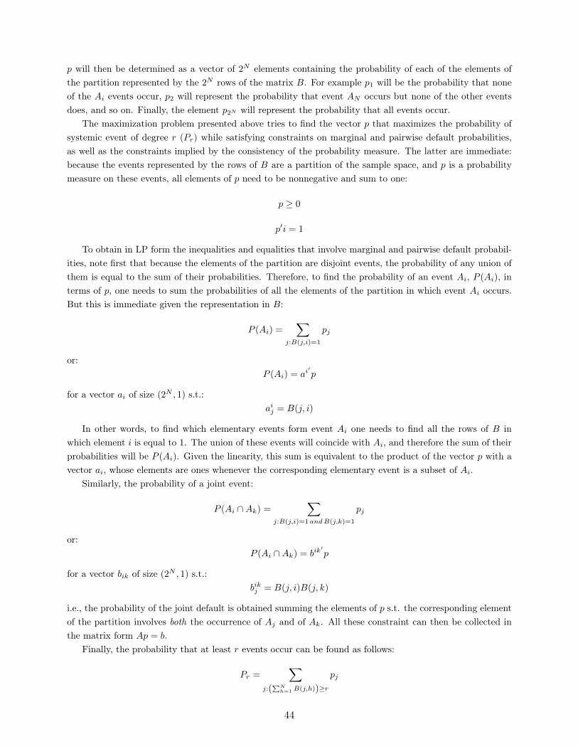
p will then be determined as a vector of 2N elements containing the probability of each of the elements ofthe partition represented by the 2N rows of the matrix B. For example p1 will be the probability that noneof the Ai events occur, p2 will represent the probability that event AN occurs but none of the other eventsdoes, and so on. Finally, the element p2N will represent the probability that all events occur.

The maximization problem presented above tries to find the vector p that maximizes the probability ofsystemic event of degree r (Pr) while satisfying constraints on marginal and pairwise default probabilities,as well as the constraints implied by the consistency of the probability measure. The latter are immediate:because the events represented by the rows of B are a partition of the sample space, and p is a probabilitymeasure on these events, all elements of p need to be nonnegative and sum to one:

p ≥ 0

p′i = 1

To obtain in LP form the inequalities and equalities that involve marginal and pairwise default probabil-ities, note first that because the elements of the partition are disjoint events, the probability of any union ofthem is equal to the sum of their probabilities. Therefore, to find the probability of an event Ai, P (Ai), interms of p, one needs to sum the probabilities of all the elements of the partition in which event Ai occurs.But this is immediate given the representation in B:

P (Ai) =∑

j:B(j,i)=1

pj

or:P (Ai) = ai

′p

for a vector ai of size (2N , 1) s.t.:aij = B(j, i)

In other words, to find which elementary events form event Ai one needs to find all the rows of B inwhich element i is equal to 1. The union of these events will coincide with Ai, and therefore the sum of theirprobabilities will be P (Ai). Given the linearity, this sum is equivalent to the product of the vector p with avector ai, whose elements are ones whenever the corresponding elementary event is a subset of Ai.

Similarly, the probability of a joint event:

P (Ai ∩Ak) =∑

j:B(j,i)=1 andB(j,k)=1

pj

or:P (Ai ∩Ak) = bik

′p

for a vector bik of size (2N , 1) s.t.:bikj = B(j, i)B(j, k)

i.e., the probability of the joint default is obtained summing the elements of p s.t. the corresponding elementof the partition involves both the occurrence of Aj and of Ak. All these constraint can then be collected inthe matrix form Ap = b.

Finally, the probability that at least r events occur can be found as follows:

Pr =∑

j:(∑N

h=1 B(j,h))≥r

pj

44

or:Pr = cr

′p

for a vector cr of size (2N , 1) s.t.:

crj = I

[N∑h=1

B(j, h) ≥ r

]where I[] is the indicator function.

Given this decomposition, the LP representation follows immediately.

B.2 - Proof of Proposition 3

Start from a symmetric LP problemmax c′p

s.t. Ap ≤ b

Suppose that p∗ is a solution to the problem. Given the definition of symmetry presented in the text, it isclear that p∗J is also a solution to the problem: c′p∗ = c′p∗J and similarly hold for every row of the constraints,for every J.

Now, construct p∗∗ as follows:

p∗∗ =1

#J

∑J

p∗J

where the first J correspond to no permutation, and J cycles across all permutations of indices A1, ..., AN .Note that it is also possible to construct p∗∗ in the following way, considering the binary representation

introduced in Proposition 2. Every bi vector has Oi ones and N − Oi zeros. Call Hi the set of all vectorsof size N that have Oi ones and N − Oi zeroes in different positions. Call bih the vector corresponding toelement h from Hi. Then, for every i, construct p∗∗ as:

p∗∗i =

(Oi

N

)−1 ∑h∈Hi

bih

From the first construction, it is clear why p∗∗ is a solution to the maximization problem, being just anaverage of solutions. Additionally, p∗∗ is symmetric, which proves the statement of the Proposition.

An example with N = 3. As explained in Proposition 2, we can construct the probability system p∗ asfollows:

p∗1 = PrA1 ∩A2 ∩A3

p∗2 = PrA1 ∩A2 ∩A3

p∗3 = PrA1 ∩A2 ∩A3

p∗4 = PrA1 ∩A2 ∩A3

p∗5 = PrA1 ∩A2 ∩A3

p∗6 = PrA1 ∩A2 ∩A3

p∗7 = PrA1 ∩A2 ∩A3

45

p∗8 = PrA1 ∩A2 ∩A3

Suppose p∗ solves the maximization problem, and construct p∗∗ as:

p∗∗1 = p∗1

p∗∗2 = p∗∗3 = p∗∗5 =p∗2 + p∗3 + p∗5

3

p∗∗4 = p∗∗6 = p∗∗7 =p∗4 + p∗6 + p∗7

3

p∗∗8 = p∗8

p∗∗ solves the maximization problem and is symmetric.

B.3 - Uniqueness of the solution and representative solution

As described in section 3, it is possible to describe the range of possible values for a particular probabilityP (A′) = v′p among the probability systems p that attain the solution to the probability bounds problem:

cmax = maxp c′rp

s.t.p ≥ 0

i′p = 1

Ap = b

(and similarly for the lower bound). To find the maximum (minimum) value of v′p at the upper bound onsystemic risk, simply solve the max (or min) problem

maxp(minp) v′p

s.t.p ≥ 0

i′p = 1

Ap = b

c′rp = cmax

To find the maximum and minimum value of v′p at the lower bound, replace the last constraint withc′rp = cmin.

Appa (2002) describes an algorithm (called AFROS) to find a “representative” solution to the bounds.Call Ep = d the set of all equality constraints in the problem, and note that the original maximizationproblem can always be rewritten with a series of equality constraints and a nonnegativity constraint for anexpanded vector p. The algorithm proceeds as follows.

1. Solve P 0 : max c′rp s.t. Ep = d, p ≥ 0. Let p = p0 be the solution to P 0.

2. Solve P 1: max d1p s.t Ep = d, p ≥ 0, c′rp = c′rp0, where d1 is a row vector with d1j = 1 if p0j = 0,

otherwise d1j = 0. If maximum value of d1p = 0, stop. There is no alternative solution. Otherwise, let

46

p = p1 be the optimal solution to P 1. Set counter q = 1

3. q = q + 1. While q < s, solve P q: max dqp s.t. Ep = d, p ≥ 0, c′rp = c′rp0, drp ≥ αr for r = 1, ..., q − 1.

dqj = 1 if pq−1j = 0, 0 otherwise, and αr are positive numbers.

4. After S steps, the “representative solution” is the average of the p from p0 to pS .

The algorithm starts from a solution p0 and looks for another solution that maximizes the sum of all andonly those elements of p that are hitting the constraint p ≥ 0 at p0. This is the sense in which p1 will be asdissimilar as possible from p0. From p1, it will repeat the same procedure to find another solution p2, and soon, with additional constraints that ensure that the algorithm never converges back to a previous solution.The average of these solutions, itself a probability system, is the “representative” solution.

B.4 Width of the bounds

Given Proposition 3, we can derive the analytical formulation of the bounds derived as a special case of thebounds presented in Boros and Prekopa (1989), section 8. Here, S1 = Nq1 and S2 = N(N−1)

2 q2. The boundsare nonlinear functions of S1 and S2 and take the following form, for 3 ≤ r ≤ N−1. Square brackets indicateinteger part.

Lower bound in the symmetric case

CallA1 = (r − 1)N − (r +N − 2)Nq1 +N(N − 1)q2

A2 = −(r − 2)Nq1 +N(N − 1)q2

and remember that q2 ≤ q1. Then,

A2 ≤ 0⇐⇒ q2 ≤(r − 2)

(N − 1)q1

A1 ≤ 0⇐⇒ q2 ≤(r +N − 2)q1 − r + 1

N − 1=

(r − 2)q1N − 1

+Nq1 − r + 1

N − 1

The bounds then can be written as follows.CASE 1: If q1 < r−1

N

• If q2 ≤ (r−2)(N−1)q1

pr ≥ 0

• If (r−2)(N−1)q1 ≤ q2 ≤ q1

pr ≥−(r − 2)Nq1 +N(N − 1)q2

(N + 1− r)N

CASE 2: If q1 > r−1N

• If q2 ≤ (r−2)q1N−1 + Nq1−r+1

N−1

i =

[N(N − 1)q2 − (r − 2)Nq1

Nq1 − (r − 1)

]

pr ≥(r − 1)(r − 2i− 2) + 2iNq1 −N(N − 1)q2

(i− r + 2)(i− r + 1)(24)

47

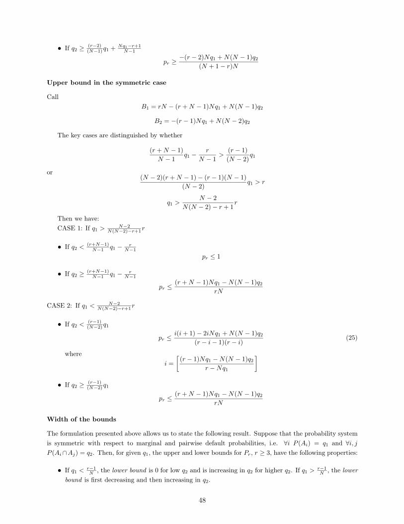
• If q2 ≥ (r−2)(N−1)q1 + Nq1−r+1

N−1

pr ≥−(r − 2)Nq1 +N(N − 1)q2

(N + 1− r)N

Upper bound in the symmetric case

CallB1 = rN − (r +N − 1)Nq1 +N(N − 1)q2

B2 = −(r − 1)Nq1 +N(N − 2)q2

The key cases are distinguished by whether

(r +N − 1)

N − 1q1 −

r

N − 1>

(r − 1)

(N − 2)q1

or(N − 2)(r +N − 1)− (r − 1)(N − 1)

(N − 2)q1 > r

q1 >N − 2

N(N − 2)− r + 1r

Then we have:CASE 1: If q1 > N−2

N(N−2)−r+1r

• If q2 <(r+N−1)N−1 q1 − r

N−1pr ≤ 1

• If q2 ≥ (r+N−1)N−1 q1 − r

N−1

pr ≤(r +N − 1)Nq1 −N(N − 1)q2

rN

CASE 2: If q1 < N−2N(N−2)−r+1r

• If q2 <(r−1)(N−2)q1

pr ≤i(i+ 1)− 2iNq1 +N(N − 1)q2

(r − i− 1)(r − i)(25)

wherei =

[(r − 1)Nq1 −N(N − 1)q2

r −Nq1

]• If q2 ≥ (r−1)

(N−2)q1

pr ≤(r +N − 1)Nq1 −N(N − 1)q2

rN

Width of the bounds

The formulation presented above allows us to state the following result. Suppose that the probability systemis symmetric with respect to marginal and pairwise default probabilities, i.e. ∀i P (Ai) = q1 and ∀i, jP (Ai∩Aj) = q2. Then, for given q1, the upper and lower bounds for Pr, r ≥ 3, have the following properties:

• If q1 < r−1N , the lower bound is 0 for low q2 and is increasing in q2 for higher q2. If q1 > r−1

N , the lowerbound is first decreasing and then increasing in q2.

48

• If q1 < N−2N(N−2)−r+1r, the upper bound is first increasing and then decreasing in q2. If q1 > N−2

N(N−2)−r+1r,the upper bound is first 1 and then decreasing in q2.

Similar results hold for q2 fixed, when q1 varies. The upper bound is concave and the lower bound is convex.Both bounds are continuous. The width of the bounds is continuous and concave, and has a maximum inthe interior of the parameter space.

Proof . Because we are maximizing or minimizing a continuous linear function over a convex set which isa continuous function of q1, and q2, the upper bound will be concave in q1 and q2 and the lower bound will beconvex, and the bounds will be continuous functions of q1 and q2. As shown above, they are piecewise linear.Note that we can check that equation (24) is decreasing in q2 because each of the linear parts are decreasingand the function is continuous. Similarly we can show that equation (25) is increasing in q2. Therefore, bylooking at the different combinations of values for r and N , we can check that for given q1, the width of thebounds is first increasing and then decreasing in q2 The same is true for fixed q2. This also implies that themaximum width, a positive concave function, is attained in the interior of the parameter space (q1, q2).

This result implies that the tightness of the bounds on systemic risk varies in a very precise way withchanges in the low-order risks. When pairwise default probabilities q2 are either very high or very lowcompared to the marginal default probabilities q1, the structure of the network is pinned down very preciselyand there is little uncertainty about systemic default risk, based on bond and CDS prices alone; differentparametric models that aggregate in different ways this low-order information will agree on an estimate ofsystemic risk. For intermediate values of q1 and q2, however, low-order probabilities are less informativeabout systemic events. The scope for modeling assumptions in aggregating low-order probabilities is greater.

Appendix C: additional pricing details

C.1 Bond pricing

In this section I show how to obtain the bond pricing formula in the text starting from the general discrete-time formulation of bond pricing in the reduced form model. Call hit the hazard rate process for i: theprobability of default in month t conditional on survival until then. Call rFt the monthly risk-free process.Call the rFt,T the realized return of the short-term risk-free security between t and T , s.t.

(1 + rFt,T ) =

T∏s=t+1

(1 + rFs

)The time t price of a risk-free zero-coupon bond of face value $1 at time T is:

δ(t, T ) = EQt

[1

1 + rFt,T

]

Call Gi(t, s) the probability of survival of firm i up to s under a certain realization of hazard rates of default,i.e.:

Gi(t, s) =

s−1∏r=t

(1− hir

)where EQ indicates the expectation taken under the risk neutral probability measure.

The price of a liquid bond j issued by firm i of face value $1, maturity T ij , coupon rate cij and recovery

49

equal to a fraction Rij of the value of a Treasury zero-coupon bond of comparable maturity is:

Bij(t, T ij) = EQt

T ij∑s=t+1

Gi(t, s)

1 + rFt,scij +

Gi(t, T ij)

1 + rFt,T+

T ij∑s=t+1

Gi(t, s− 1)his−11 + rFt,s

Rij

In this paper I consider only senior unsecured bonds of different coupons and maturities, so I assume that

the recovery rate is the same for all bonds and that it is also the same for similar bonds of other firms in thefinancial industry, i.e. Rij = R.

We can then add a liquidity process γit , assumed to be the same for all bonds of equal seniority offirm i. Following Duffie (1999), this liquidity cost will appear in the bond pricing equation as a per-periodproportional cost incurred while holding the bond.

In theory, it is possible to write down a parametric version of the (generally not independent) processesthat govern the evolution of rFt ,ht, γt, and additionally a time-varying recovery rate. Examples of this canbe found in Duffie and Singleton (1997) and Longstaff, Mithal and Neis (2005). In this paper, I use asimplified pricing model that assumes that, for any given firm, the prices of all of its bonds are determinedindependently at each time t, under the assumption that from time t onwards ht+s and γt+s will be constantand equal to ht and γt, respectively. This is just an approximation, because prices do not take into accountthat at each future date these parameters are going to be revised, since at every future date t+ r prices willbe recomputed assuming a constant hazard rate and liquidity process from t+ r on at new levels, ht+r andγt+r. I discretize the model to a monthly horizon, and I assume that coupons are paid monthly. Furtherassuming independence of the risk-free rate process from all other processes (under Q) we obtain:

Bij(t, T ij) = cij

T ij∑s=t+1

δ(t, s)(1− hit)s−t(1− γit)s−t+

+δ(t, T ij)(1− hit)Tij−t(1− γit)T

ij−t +R

T ij∑s=t+1

δ(t, s)(1− hit)s−t−1(1− γit)s−t−1hit

C.2 - Additional details of CDS contracts

Besides those considered explicitly in this paper, there are other elements of CDS contracts that potentiallyaffect their spreads.

First, liquidity of the CDS market could influence the CDS spreads, just as bond liqudiity is known toaffect bond prices. In this paper, I explicitly take into account liquidity premia in bond prices, but not inCDS spreads. For the case of CDSs, liquidity is much less likely to be an issue, especially because they requiremuch less capital at origination and they are not in fixed supply.42

Also, I abstract from restructuring clauses and the cheapest-to-deliver option sometimes present in CDScontracts. A restructuring clause (under which payment is triggered for simple debt restructuring, in additionto bankruptcy) is more frequent for European bonds, and this results in the contract being triggered in casesclose to the Chapter 11 for the US. Berndt, Jarrow and Kang (2007) estimate that the presence of suchclause increases the value of the CDSs by 6-8%, and all the results in this paper are robust to an adjustmentof CDS spreads of that magnitude. The value of the cheapest-to-deliver option (which allows the buyer todeliver to the seller the cheapest of the defaulted bonds of the same seniority as the reference bond) will besmall relative to the CDS spread as long as in default all senior unsecured bonds have similar recovery rates.

42For an additional discussion of this and on the supporting evidence, see Blanco, Brennan and Marsh(2003,2005).

50

Additionally, as observed in the Delphi and Calpine defaults in 2005, the high demand for the cheapest bondsmight determine shortages of such securities and therefore, anticipating this, a reduction in the ex-ante valueof the option.43

C.3 - CDS pricing approximation

Start from the discretized pricing equation with constant hazard and risk-free rates, starting from period 0for notational simplicity.

T∑s=1

δ(0, s− 1)(1− P (Ai ∪Aj))s−1zji =

=

[T∑s=1

(1− P (Ai ∪Aj))s−1(P (Ai)− (1− S)P (Ai ∩Aj))δ(0, s)(1−R)

]We can rewrite the equation as:

zij(1−R)

=

[∑Ts=1 δ(0, s)(1− P (Ai ∪Aj))s−1(P (Ai)− (1− S)P (Ai ∩Aj))

]∑Ts=1 δ(0, s− 1)(1− P (Ai ∪Aj))s−1

and then approximate the right hand side around P (Ai) = 0, P (Aj) = 0, P (Ai ∩ Aj) = 0, rememberingthat

P (Ai ∪Aj) = P (Ai) + P (Aj)− P (Ai ∩Aj)

To obtain the approximation, note that while we cannot vary P (Ai) and P (Ai∩Aj) independently around0, we can rewrite the expression in terms of:

πi = P (Ai ∩Aj)

πj = P (Ai ∩Aj)

πij = P (Ai ∩Aj)

which can be varied independently of each other. The right-hand side (call it G, and call G(0) the functionat the approximation point) can then be written as:

G =

[∑Ts=1 δ(0, s)(1− πi − πj − πij)s−1(πi + πij − (1− S)πij)

]∑Ts=1 δ(0, s− 1)(1− πi − πj − πij)s−1

First, note that G(0) = 0. Second, take Gπi(0):

Gπi(0) =

ddπi

[∑Ts=1 δ(0, s)(1− πi − πj − πij)s−1(πi + πij − (1− S)πij)

] [∑Ts=1 δ(0, s− 1)(1− πi − πj − πij)s−1

]+[∑T

s=1 δ(0, s− 1)(1− πi − πj − πij)s−1]2

[∑Ts=1 δ(0, s)(1− πi − πj − πij)s−1(πi + πij − (1− S)πij)

]ddπi

[∑Ts=1 δ(0, s− 1)(1− πi − πj − πij)s−1

][∑T

s=1 δ(0, s− 1)(1− πi − πj − πij)s−1]2

43De Wit (2006).

51

Note that the second part is 0 and at the approximation point, and at that point we have:

d

dπi

[(1− πi − πj − πij)s−1(πi + πij − (1− S)πij)

]=

d

dπi(1− πi − πj − πij)s−1 [(πi + πij − (1− S)πij)] + (1− πi − πj − πij)s−1

d

dπi[(πi + πij − (1− S)πij)] = 1

So we have:

Gπi(0) =

∑Ts=1 δ(0, s)∑T

s=1 δ(0, s− 1)

Similarly:

Gπj(0) =

∑Ts=1 δ(0, s)

ddπj

[(1− πi − πj − πij)s−1(πi + πij − (1− S)πij)

] [∑Ts=1 δ(0, s− 1)

][∑T

s=1 δ(0, s− 1)]2

withd

dπj

[(1− πi − πj − πij)s−1(πi + πij − (1− S)πij)

]=[

d

dπj(1− πi − πj − πij)s−1

][(πi + πij − (1− S)πij)] = 0

so thatGπj

(0) = 0

Finally we get:

Gπij(0) =

∑Ts=1 δ(0, s)∑T

s=1 δ(0, s− 1)S

So that:

G '∑Ts=1 δ(0, s)∑T

s=1 δ(0, s− 1)[πi + Sπij ] =

∑Ts=1 δ(0, s)∑T

s=1 δ(0, s− 1)[πi + πij − (1− S)πij ]

=

∑Ts=1 δ(0, s)∑T

s=1 δ(0, s− 1)[P (Ai)− (1− S)P (Ai ∩Aj)]

The result is:

zij(1−R)

'

[∑Ts=1 δ(0, s)

][∑T

s=1 δ(0, s− 1)] (P (Aj)− (1− S)P (Ai ∩Aj))

It is important to check the accuracy of the approximation for a realistic range of parameters. For severaldifferent points in time (every 50 days) between 1/1/2007 and 3/31/2009, I compare the correct spread andthe approximated spread, computed using the US yield curve at that time, considering:

• different values of P (Aj): between 0 and the maximum probability implied by bond data under noliquidity assumptions (maxjhj(0)).

• different values of P (Ai ∩Aj): between 0 and P (Aj)

• different values of R and S: between 0.1 and 0.4.

In all these simulations, the approximation error is between 0.2% and 0.3% of the true value of the CDSspread.

52

Appendix D - Details on the Robustness Tests

D.1 - Assumptions on S

The recovery rate of a CDS in case of double default, S, affects positively the value of that security. Inaddition, a higher recovery rate S implies a higher sensitivity of the CDS spreads to changes in the jointdefault risk. A recovery rate of zero (S = 0) means that counterparty risk has the highest impact on CDSspreads, while a recovery rate of 1 means that joint default risk has no effect on the spread.

To understand the effect of assumptions about S on the measure of systemic risk presented in this paper,remember that the upper bound on systemic risk is attained by the most correlated probability system thatsatisfies the constraints:

P (Ai) ≤ hi(γit)

P (Ai)− (1− S)

1

N − 1

∑j 6=i

P (Ai ∩Aj)

= bi

where bi = zi[∑T

s=1 δ(0,s−1)][∑T

s=1 δ(0,s)](1−R)

44.

Intuitively, for a given S, one can obtain the most correlated probability system by setting P (Ai) as highas possible (up to the constraint hi(γit)) for all banks and then increasing the term 1

N−1∑i 6=j P (Ai ∩ Aj)

to match the CDS spreads (bi). Counterparty risk would explain the whole bond/CDS basis, and a higherrecovery rate S would imply that a higher joint default probability is needed to match it, increasing the upperbound on systemic risk. This intuitive reasoning, however, does not take into account the internal restrictionsof consistency of the probability system. These can be best understood in the context of a symmetric network.

For a symmetric network, call the marginal probability of default of each bank q1 and the pairwise jointprobabilities of default of each pair q2. The previous constraints become:

q1 ≤ h

q1 − (1− S)q2 = b

where h is the (common) upper bound on the marginal probability of default and b is the (common) bi.To maximize systemic risk, we would intuitively set q1 = h, and then q2 will be set to match CDS spreads:

q2 =q1 − b1− S

(26)

For given q1, q2 is increasing in S, as is systemic risk. This captures the intuition that a higher recovery rateof CDSs implies that higher counterparty risk is needed to explain the same bond/CDS basis.

In fact, this effect is at play only when S is small enough. As S grows, q2 keeps increasing, and at somepoint it will reach the level q2 = q1. At that point, the internal consistency of the probability system kicksin, preventing further increases: it would violate the implicit constraint that q2 ≤ q1.

What happens then if S increases further? The only way to satisfy the constraints is to lower q1 below

44I focus on the upper bound for the probability of at least r > 1 events occurring. Following the analysisreported in section 3, the same argument holds for the lower bound for the probability that at least 1institution defaults, since that is achieved for a very correlated system. It is easy to see why the results forthe lower bound for r > 1 and the upper bound for r = 1 do not depend on S: these bounds look for theleast correlated system, which can always be obtained by setting the marginal default probabilities at thelevels implied by the CDS spreads and attributing the bond/CDS basis entirely to liquidity.

53

h: for q1 = h there might exist no probability systems able to satisfy both constraints: matching the CDSspread and satisfying internal consistency. Instead, with a lower q1, it is possible to set q2 to be equal to q1and satisfy the CDS constraint, so that:

q2 = q1 =b

S

which is decreasing in S. This means that for large enough values of S, the bond/CDS basis is too large tobe explained by counterparty risk. Even at the upper bound on systemic risk, liquidity has to explain partof the basis. In a symmetric system, then, the bounds on systemic risk first increase and then decrease withS.

These forces play out in similar but nonlinear ways for asymmetric networks. In that case, the asymmetryin the bond/CDS basis across banks means that the upper bounds on marginal probabilities (that are obtainedfrom bond prices) will bind for some banks and not for others. The overall effect on the bounds is difficult todescribe analytically but can be tested numerically. The results, described in the text, are reported in Table3.

D.2 - Stochastic recovery rate

This section shows that if recovery rates are stochastic, the change in bond and CDS prices can be decomposedas follows. Starting from the prices obtained in the case of a constant recovery rate R (section 4), the pricesare first adjusted by changing the recovery rate to a lower value RL. In addition, the price of the bondand the present value of CDS payments are shifted in opposite directions by an amount Y (to a first orderapproximation).

To see this, assume that the recovery rate on bonds is RH if one bank defaults alone but is RL if morethan one bank defaults at the same time. Call Xi = ∪k 6=iAk the event of at least one default among thebanks different from i, and similarly Xij = ∪k 6=i,jAk. Call BR(0, T ) the price of a bond under the assumptionof constant recovery rate R and BRL,RH

(0, T ) the price of a bond with stochastic recovery rate describedabove, and similarly for the CDS spreads. Then, it is easy to see that (setting liquidity to 0 for simplicity)

BRL,RH(0, T ) = c

(T∑t=1

δ(0, t)(1− P (Ai))t

)+ δ(0, T )(1− P (Ai))

T+

+RH

(T∑t=1

δ(0, t)(1− P (Ai))t−1P (Ai ∩Xi))

)+RL

(T∑t=1

δ(0, t)(1− P (Ai))t−1P (Ai ∩Xi)

)while the CDS spread solves:

T∑s=1

δ(0, s− 1)(1− P (Ai ∪Aj))s−1zRL,RH ,ji =

=

T∑s=1

(1− P (Ai ∪Aj))s−1δ(0, s)[P (Ai ∩Aj ∩Xij)(1−RH)

+P (Ai ∩Aj ∩Xij)(1−RL) + P (Ai ∩Aj)(1−RL)S]

Now, rewrite bond prices as:

BRL,RH(0, T ) = c

(T∑t=1

δ(0, t)(1− P (Ai))t

)+ δ(0, T )(1− P (Ai))

T+

54

+(RH−RL)

(T∑t=1

δ(0, t)(1− P (Ai))t−1P (Ai ∩Xi)

)+RL

(T∑t=1

δ(0, t)(1− P (Ai))t−1 [P (Ai ∩Xi) + P (Ai ∩Xi)

])

Noting that the term P (Ai ∩Xi) + P (Ai ∩Xi) = P (Ai), we can rewrite

BRL,RH(0, T ) = c

(T∑t=1

δ(0, t)(1− P (Ai))t

)+

+δ(0, T )(1− P (Ai))T +RL

(T∑t=1

δ(0, t)(1− P (Ai))t−1P (Ai)

)+ Ybond

or:BRL,RH

(0, T ) = BRL(0, T ) + Ybond

where

Ybond =

T∑t=1

δ(0, t)(1− P (Ai))t−1P (Ai ∩Xi)(RH −RL)

The price of the bond is now equal to the price of the bond in case that the recovery rate is constant andequal to RL plus the last term, which is the present value of the additional recoveries in case i defaults alone.

A similar fromula holds for CDS spreads. Since P (Ai ∩Aj ∩Xij) = P (Ai ∩Xi), we can rewrite the CDSspread as

T∑s=1

δ(0, s− 1)(1− P (Ai ∪Aj))s−1zRL,RH ,ji =

=

T∑s=1

(1− P (Ai ∪Aj))s−1δ(0, s)[P (Ai ∩Aj ∩Xij)(1−RH)− P (Ai ∩Aj ∩Xij)(1−RL)

+P (Ai ∩Aj ∩Xij)(1−RL) + P (Ai ∩Aj ∩Xij)(1−RL) + P (Ai ∩Aj)(1−RL)S]

=

T∑s=1

(1− P (Ai ∪Aj))s−1δ(0, s)[P (Ai ∩Aj ∩Xij)(RL −RH)

+(1−RL)(P (Ai ∩Aj ∩Xij) + P (Ai ∩Aj ∩Xij) + P (Ai ∩Aj)S

)]

SinceP (Ai ∩Aj ∩Xij) + P (Ai ∩Aj ∩Xij) + P (Ai ∩Aj)S =

= P (Ai ∩Aj) + P (Ai ∩Aj)S = P (Ai)− (1− S)P (Ai ∩Aj)

we can write:T∑s=1

δ(0, s− 1)(1− P (Ai ∪Aj))s−1zRL,RH ,ji =

=

T∑s=1

(1− P (Ai ∪Aj))s−1δ(0, s)[P (Ai ∩Aj ∩Xij)(RL −RH)

+(1−RL)(P (Ai)− (1− S)P (Ai ∩Aj))]

=

T∑s=1

(1− P (Ai ∪Aj))s−1δ(0, s) (P (Ai)− (1− S)P (Ai ∩Aj)) (1−RL)

− YCDS

55

or:

T∑s=1

δ(0, s− 1)(1− P (Ai ∪Aj))s−1zRL,RH ,ji =

T∑s=1

δ(0, s− 1)(1− P (Ai ∪Aj))s−1zRL,ji − YCDS

where

YCDS =

T∑s=1

(1− P (Ai ∪Aj))s−1δ(0, s)P (Ai ∩Xi)(RH −RL)

Now we can show that when probabilities are small, YCDS and Ybond are approximately the same. To dothis, rewrite the two formulas in terms of the following probabilities: πi = P (Ai ∩ Aj ∩Xij) = P (Ai ∩Xi),πj = P (Aj ∩ Ai), πij = P (Ai ∩ Aj), πk = P (Ai ∩ Aj ∩ Xij). Note that these three sets are disjoint andtherefore if the probabilities of the other events are small we can vary them independently of each other.Then,

YCDS =

T∑s=1

(1− πi − πj − πij − πk)s−1δ(0, s)πi(RH −RL)

Ybond =

T∑s=1

(1− πi − πij − πk)s−1δ(0, s)πi(RH −RL)

Approximating each of these equations around πi = πj = πij = πk = 0, we note that:

YCDS(0) = 0

d

dπiYCDS(0) =

T∑s=1

δ(0, s)(RH−RL)

[(d

dπi(1− πi − πj − πij − πk)s−1

)πi +

((1− πi − πj − πij − πk)s−1

) d

dπiπi

]0

=

T∑s=1

δ(0, s)(RH −RL)

andd

dπjYCDS(0) =

d

dπijYCDS(0) =

d

dπkYCDS(0) = 0

And similarly for Ybond: so, to a first approximation, YCDS = Ybond.

D.3 - Alternative pricing model

Suppose that at every time t agents prices bonds assuming for the life of the bond a deterministic hazardrate of the form:

ht+s = (1− ρt)ht + ρtht+s−1

with a certain ht, ρt, and ht determined at time t.Note that

ht+s = (1− ρt)(1 + ...+ ρs−1t )ht + ρstht

= (1− ρt)1− ρst1− ρt

ht + ρstht

= (1− ρst )ht + ρstht

for s ≥ t.

56

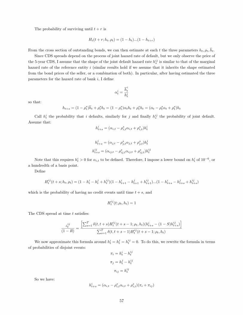
The probability of surviving until t+ r is

Ht(t+ r;ht, ρt) = (1− ht)...(1− ht+r)

From the cross section of outstanding bonds, we can then estimate at each t the three parameters ht, ρt, ht.Since CDS spreads depend on the process of joint hazard rate of default, but we only observe the price of

the 5-year CDS, I assume that the shape of the joint default hazard rate hijs is similar to that of the marginalhazard rate of the reference entity i (similar results hold if we assume that it inherits the shape estimatedfrom the bond prices of the seller, or a combination of both). In particular, after having estimated the threeparameters for the hazard rate of bank i, I define

αit =hi

t

hit

so that:ht+s = (1− ρst )ht + ρstht = (1− ρst )αtht + ρstht = (αt − ρstαt + ρst )ht

Call hit the probability that i defaults, similarly for j and finally hijs the probability of joint default.Assume that:

hit+s = (αi,t − ρsi,tαi,t + ρsi,t)hit

hjt+s = (αj,t − ρsj,tαj,t + ρsj,t)hjt

hijt+s = (αij,t − ρsij,tαij,t + ρsij,t)hijt

Note that this requires hit > 0 for αi,t to be defined. Therefore, I impose a lower bound on hit of 10−6, ora hundredth of a basis point.

Define

Hijt (t+ s;ht, ρt) = (1− hit − h

jt + hijt )(1− hit+1 − h

jt+1 + hijt+1)...(1− hit+s − h

jt+s + hijt+s)

which is the probability of having no credit events until time t+ s, and

Hijt (t; ρt, ht) = 1

The CDS spread at time t satisfies:

zijt(1−R)

=

[∑Ts=1 δ(t, t+ s)Hij

t (t+ s− 1; ρt, ht)(hit+s − (1− S)hijt+s)

]∑Ts=1 δ(t, t+ s− 1)Hij

t (t+ s− 1; ρt, ht)

We now approximate this formula around hit = hjt = hijt = 0. To do this, we rewrite the formula in termsof probabilities of disjoint events:

πi = hit − hijt

πj = hjt − hijt

πij = hijt

So we have:hit+s = (αi,t − ρsi,tαi,t + ρsi,t)(πi + πij)

57

hjt+s = (αj,t − ρsj,tαj,t + ρsj,t)(πj + πij)

hijt+s = (αij,t − ρsij,tαij,t + ρsij,t)πij

Call

G =

[∑Ts=1 δ(t, t+ s)Hij

t (t+ s− 1; ρt, ht)(hit+s − (1− S)hijt+s)

]∑Ts=1 δ(t, t+ s− 1)Hij

t (t+ s− 1; ρt, ht)

We can start by noting that at the approximation point, πi = πj = πij = 0, we have:

(hit+s − (1− S)hijt+s)|0 = 0

Hijt (t+ s− 1; ρt, ht)|0 = 1

We then have, for each of the π

d

dπG|0 =

ddπ

[∑Ts=1 δ(t, t+ s)Hij

t (t+ s− 1; ρt, ht)(hit+s − (1− S)hijt+s)

] [∑Ts=1 δ(t, t+ s− 1)Hij

t (t+ s− 1; ρt, ht)]

[∑Ts=1 δ(t, t+ s− 1)Hij

t (t+ s− 1; ρt, ht)]2

−

[∑Ts=1 δ(t, t+ s)Hij

t (t+ s− 1; ρt, ht)(hit+s − (1− S)hijt+s)

]ddπ

[∑Ts=1 δ(t, t+ s− 1)Hij

t (t+ s− 1; ρt, ht)]

[∑Ts=1 δ(t, t+ s− 1)Hij

t (t+ s− 1; ρt, ht)]2 |0

The second term, at the approximation point, is always 0. We can reduce the derivative to:

d

dπG|0 =

∑Ts=1 δ(t, t+ s)

[ddπH

ijt (t+ s− 1; ρt, ht)

](hit+s − (1− S)hijt+s) +Hij

t (t+ s− 1; ρt, ht)ddπ (hit+s − (1− S)hijt+s)

∑Ts=1 δ(t, t+ s− 1)

|0

which in turn becomesd

dπG|0 =

∑Ts=1 δ(t, t+ s) d

dπ (hit+s − (1− S)hijt+s)∑Ts=1 δ(t, t+ s− 1)

|0

Now,hit+s = (αi,t − ρsi,tαi,t + ρsi,t)(πi + πij)

hjt+s = (αj,t − ρsj,tαj,t + ρsj,t)(πj + πij)

hijt+s = (αij,t − ρsij,tαij,t + ρsij,t)πij

d

dπ(hit+s − (1− S)hijt+s) =

=d

dπ((αi,t − ρsi,tαi,t + ρsi,t)(πi + πij)− (1− S)(αij,t − ρsij,tαij,t + ρsij,t)πij)

So that:d

dπi(hit+s − (1− S)hijt+s) = (αi,t − ρsi,tαi,t + ρsi,t)

andd

dπij(hit+s − (1− S)hijt+s) = (αi,t − ρsi,tαi,t + ρsi,t)− (1− S)(αij,t − ρsij,tαij,t + ρsij,t)

d

dπj(hit+s − (1− S)hijt+s) = 0

58

Therefore we have:d

dπG|0 =

∑Ts=1 δ(t, t+ s) d

dπ (hit+s − (1− S)hijt+s)∑Ts=1 δ(t, t+ s− 1)

|0

G '∑Ts=1 δ(t, t+ s)

[(αi,t − ρsi,tαi,t + ρsi,t)

]πi +

[(αi,t − ρsi,tαi,t + ρsi,t)− (1− S)(αij,t − ρsij,tαij,t + ρsij,t)

]πij∑T

s=1 δ(t, t+ s− 1)

=

∑Ts=1 δ(t, t+ s)(αi,t − ρsi,tαi,t + ρsi,t)h

it − (1− S)(αij,t − ρsij,tαij,t + ρsij,t)h

ijt∑T

s=1 δ(t, t+ s− 1)

Calling

Gi =

∑Ts=1 δ(t, t+ s)(αi,t − ρsi,tαi,t + ρsi,t)∑T

s=1 δ(t, t+ s− 1)

and

Gij =

∑Ts=1 δ(t, t+ s)(αij,t − ρsij,tαij,t + ρsij,t)∑T

s=1 δ(t, t+ s− 1)

we obtain:zijt

(1−R)' Gihit − (1− S)Gijh

ijt

Summing over counterparties, we have:

(N − 1)zitGi(1−R)

' (N − 1)hit − (1− S)∑j 6=i

GijGi

hijt

which is again linear in the marginal and pairwise default probabilities and can be used in the LPformulation. To impose that CDS spreads inherit the shape of the hazard rates estimated from bonds, wecan assume αij,t = αi,t and ρij,t = ρi,t. Note that this reduces the CDS spread to a function of only oneparameter: hijt .

D.4 Currency assumptions

To simplify, consider one-period bonds and CDSs denominated in different currencies. Callmse the stochasticdiscount factor of a US investor in state (s, e) where s indicates whether default of firm i (s = i or 0) occursor not and e is the exchange rate. Assume that international bond and CDS markets are not segmented, sothat m prices all assets. Call f(s, e) the joint density function s and e. To simplify notation, rewrite f(s, e)

as:f(s, e) = πsfs(e)

Note thatπ0E[mse|s = 0] + πiE[mse|s = i] = E[mse]

For a dollar-denominated risky bond (R is the recovery rate), the dollar price is:

p$i = π0E[mse|s = 0] +RπiE[mse|s = i] = E[mse]− (1−R)πiE[mse|s = i]

Now consider a euro-denominated bond issued by the same firm, and of equal seniority. Calling e0 thetime-0 exchange rate, we obtain:

pEi e0 = π0E[e ·m0e|s = 0] +RπiE[e ·mie|s = i]

59

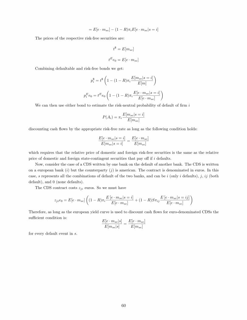
= E[e ·mse]− (1−R)πiE[e ·mse|s = i]

The prices of the respective risk-free securities are:

t$ = E[mse]

tEe0 = E[e ·mse]

Combining defaultable and risk-free bonds we get:

p$i = t$(

1− (1−R)πiE[mse|s = i]

E[m]

)

pEi e0 = tEe0

(1− (1−R)πi

E[e ·mse|s = i]

E[e ·mse]

)We can then use either bond to estimate the risk-neutral probability of default of firm i

P (Ai) = πiE[mse|s = i]

E[mse]

discounting cash flows by the appropriate risk-free rate as long as the following condition holds:

E[e ·mse|s = i]

E[mse|s = i]=E[e ·mse]

E[mse]

which requires that the relative price of domestic and foreign risk-free securities is the same as the relativeprice of domestic and foreign state-contingent securities that pay off if i defaults.

Now, consider the case of a CDS written by one bank on the default of another bank. The CDS is writtenon a european bank (i) but the counterparty (j) is american. The contract is denominated in euros. In thiscase, s represents all the combinations of default of the two banks, and can be i (only i defaults), j, ij (bothdefault), and 0 (none defaults).

The CDS contract costs zji euros. So we must have

zjie0 = E[e ·mse]

((1−R)πi

E [e ·mse|s = i]

E[e ·mse]+ (1−R)Sπij

E [e ·mse|s = ij]

E[e ·mse]

)Therefore, as long as the european yield curve is used to discount cash flows for euro-denominated CDSs thesufficient condition is:

E[e ·mse|s]E[mse|s]

=E[e ·mse]

E[mse]

for every default event in s.

60

Tables

Avg valid bonds 2004 2005 2006 2007 2008 2009 2010Abn Amro 3.3 1.8 2.2 4.0 4.4 3.0 3.5 5.3Bank of America 32.3 17.5 25.4 29.3 32.9 35.3 41.8 55.8Barclays 14.8 3.1 3.0 2.4 2.5 9.1 38.5 78.0Bear Stearns 11.4 7.2 9.8 12.6 15.3 15.4 - -Bnp Paribas 7.0 0.5 2.0 3.0 3.9 6.7 18.0 22.6Citigroup 36.5 21.6 24.3 31.7 40.0 43.2 49.5 54.5Credit Suisse 5.4 1.9 2.3 2.8 2.7 5.0 11.6 17.4Deutsche Bank 42.1 5.3 10.4 42.3 68.9 54.4 58.8 67.9Goldman Sachs 39.6 19.3 26.1 34.3 40.4 49.0 57.0 63.0JP Morgan 17.3 6.6 11.1 14.0 17.4 22.2 27.4 27.9Lehman Brothers 20.1 10.5 15.2 20.5 26.5 31.4 - -Merrill Lynch 35.7 22.7 33.0 38.4 43.0 44.0 - -Morgan Stanley 25.5 12.5 14.6 17.5 22.2 30.0 45.0 49.0UBS 8.2 0.3 0.7 1.0 3.1 8.3 22.4 36.6Wachovia 6.1 2.9 3.5 5.7 7.4 9.1 7.7 7.3

Table 1

Note: first column reports average number of bonds for each institution that are used for the estimation of marginal default probabilities. Columns 2-8 break this number down by year.

Avg CDS spread Std CDS spread Min spread Max spread Avg basis Std basis Min basis Max basisAbn Amro 45.8 46.1 5.0 190.5 -46.2 44.4 -248.2 34.6Bank of America 66.5 71.7 7.4 390.7 -71.9 64.8 -412.5 217.5Barclays 54.3 60.0 5.5 261.9 -41.2 60.1 -324.8 111.6Bear Stearns 54.2 69.7 18.0 736.9 -53.6 24.6 -298.0 40.6Bnp Paribas 33.8 32.2 5.4 163.9 -53.9 49.7 -321.8 86.8Citigroup 100.4 129.7 6.5 638.3 -76.5 88.1 -804.6 59.2Credit Suisse 53.0 51.3 9.0 261.4 -50.5 44.0 -276.6 52.6Deutsche Bank 49.8 45.1 8.9 190.0 -24.4 27.6 -174.2 65.2Goldman Sachs 84.2 86.4 17.2 579.3 -79.0 91.3 -502.4 75.1JP Morgan 53.1 42.8 10.9 227.3 -76.5 57.9 -322.2 32.1Lehman Brothers 70.7 86.9 18.0 701.7 -61.9 44.5 -540.0 10.9Merrill Lynch 59.9 71.9 14.4 447.7 -51.7 40.4 -200.0 26.2Morgan Stanley 112.5 144.2 16.6 1385.6 -82.6 107.3 -1256.5 223.2UBS 59.3 72.4 4.2 357.2 -65.4 58.5 -343.5 34.2Wachovia 73.9 93.5 9.3 1487.7 -87.2 120.1 -2509.8 88.0

Table 2

Note: table reports descriptive characteristics on the CDS spread and the yield spread for the 15 institutions in the sample, in basispoints per year. The yield spread is computed as the linearly interpolated yield for a 5-year maturity bond in excess of the correspondingTreasury rate.

61

2007 Jan 2008 to Bear

Bear to Lehman

Month after

Lehman

Oct 2008 to April 2009

After April 2009

Start 1/1/07 1/1/08 3/16/08 9/15/08 10/16/08 5/1/09

R S End 12/31/07 3/15/08 9/12/08 10/15/08 4/30/09 6/10/10

0.10 0.10 50.4 178.0 168.8 298.1 221.7 133.00.10 0.30 50.4 178.0 168.8 298.1 221.7 133.00.10 0.40 50.4 178.0 168.8 298.1 221.7 133.00.10 0.70 50.4 178.0 168.8 298.1 221.7 133.00.10 0.90 50.4 178.0 168.8 298.1 221.7 133.00.10 1.00 50.4 178.0 168.8 298.1 221.7 133.00.30 0.30 64.8 228.9 217.0 383.3 285.0 171.10.30 0.40 64.8 228.9 217.0 383.3 285.0 171.10.30 0.70 64.8 228.9 217.0 383.3 285.0 171.10.30 0.90 64.8 228.9 217.0 383.3 285.0 171.10.30 1.00 64.8 228.9 217.0 383.3 285.0 171.10.40 0.40 75.6 267.1 253.2 447.1 332.5 199.60.40 0.70 75.6 267.1 253.2 447.1 332.5 199.60.40 0.90 75.6 267.1 253.2 447.1 332.5 199.60.40 1.00 75.6 267.1 253.2 447.1 332.5 199.6

64.8 229.0 217.1 383.6 285.2 171.149.4 166.7 156.7 278.7 182.7 102.246.5 166.4 156.6 278.7 183.3 96.565.0 228.9 217.0 383.3 285.8 171.365.0 228.9 217.0 383.3 285.8 171.335.2 112.0 162.2 579.0 216.9 51.9

2007 Jan 2008 to Bear

Bear to Lehman

Month after

Lehman

Oct 2008 to April 2009

After April 2009

Start 1/1/07 1/1/08 3/16/08 9/15/08 10/16/08 5/1/09

R S End 12/31/07 3/15/08 9/12/08 10/15/08 4/30/09 6/10/10

0.10 0.10 2.2 2.3 15.7 24.3 49.1 30.90.10 0.30 2.4 2.5 17.3 25.7 48.8 31.20.10 0.40 2.5 2.6 18.2 26.2 48.6 31.20.10 0.70 2.8 2.9 20.0 27.7 47.2 30.60.10 0.90 3.3 3.3 21.5 28.4 46.0 29.70.10 1.00 12.6 44.5 42.2 70.0 55.4 33.30.30 0.30 3.3 3.5 24.7 42.1 64.8 40.60.30 0.40 3.4 3.7 25.6 42.5 64.2 40.50.30 0.70 3.7 4.1 27.9 43.7 62.0 39.60.30 0.90 4.1 4.6 29.5 44.3 60.6 38.30.30 1.00 16.2 57.2 54.3 90.0 71.2 42.80.40 0.40 4.0 4.4 32.0 54.0 76.8 47.50.40 0.70 4.3 5.0 34.7 54.0 74.0 46.30.40 0.90 4.8 5.7 36.1 53.3 72.0 44.80.40 1.00 18.9 66.8 63.3 104.9 83.1 49.9

2.3 2.6 19.3 42.5 58.1 28.01.3 0.8 11.3 36.9 36.0 17.01.4 1.0 16.6 39.6 42.1 16.65.3 5.0 32.4 50.3 74.5 44.75.2 5.1 32.9 50.1 75.6 44.82.6 4.7 18.7 49.5 36.7 10.1

US banks, larger transUS banks

Reweight top 5 banks

Table 3a: max P1

Model Average level of the bounds (bp per month)

Using swap rates

Alternative bond model

Reweight, decreasingAlternative bond model

Table 3b: max P4

Model Average level of the bounds (bp per month)

Using swap ratesUS banks

US banks, larger transReweight top 5 banksReweight, decreasing

62

2007 Jan 2008 to Bear

Bear to Lehman

Month after

Lehman

Oct 2008 to April 2009

After April 2009

Start 1/1/07 1/1/08 3/16/08 9/15/08 10/16/08 5/1/09

R S End 12/31/07 3/15/08 9/12/08 10/15/08 4/30/09 6/10/10

0.10 0.10 42.6 164.9 121.7 221.9 109.8 62.30.10 0.30 42.0 164.3 117.4 217.3 101.3 56.10.10 0.40 41.8 163.8 115.0 214.7 97.0 53.00.10 0.70 40.9 162.2 107.2 205.8 85.8 44.40.10 0.90 39.1 160.6 101.1 202.8 80.6 40.30.10 1.00 7.4 27.3 25.1 84.7 41.3 22.60.30 0.30 53.9 210.3 146.4 252.2 125.9 71.30.30 0.40 53.6 209.5 143.1 248.0 120.4 67.30.30 0.70 52.5 206.6 132.9 237.4 106.5 56.60.30 0.90 50.9 204.8 125.3 232.8 99.4 51.60.30 1.00 9.5 35.1 32.2 108.9 53.1 29.00.40 0.40 62.4 243.7 161.9 281.8 135.8 77.90.40 0.70 61.2 241.3 149.8 273.5 120.1 65.60.40 0.90 59.7 238.9 142.3 268.4 111.1 59.70.40 1.00 11.1 40.9 37.6 127.0 61.9 33.8

56.6 217.0 156.1 258.2 141.5 97.843.3 157.9 117.0 187.0 110.6 62.339.8 154.1 109.8 168.8 100.6 57.450.4 204.8 128.2 243.5 121.5 67.550.9 204.4 128.2 249.7 121.1 64.625.2 92.4 107.5 397.8 121.3 26.6

Table 3c: min P1

Reweight, decreasingAlternative bond model

Note: Table reports the average value of the bounds on monthly P1 (probability that at least one bankdefaults) and P4 (probability that at least four banks default) for different nonoverlapping periods, underdifferent assumptions discussed in the text. The lower bound for P4 is 0 throughout.

Model Average level of the bounds (bp per month)

Using swap ratesUS banks

US banks, larger transReweight top 5 banks

63

Figures

2004

2005

2006

2007

2008

2009

2010

0

0.01

0.02

0.03

0.04

0.05

0.06

0.07

Av

erag

e Yi

eld

Spre

adAv

erag

e C

DS

spre

adN

egat

ive

Basi

s (re

scal

ed)

Figure 1: Average 5-year bond yield and CDS spread for the 15 financial intermediaries most active in theCDS market, together with the (rescaled) difference between the two (the negative bond/CDS basis). Thebond yield is obtained by interpolating bond yields at the 5 year maturity.

64

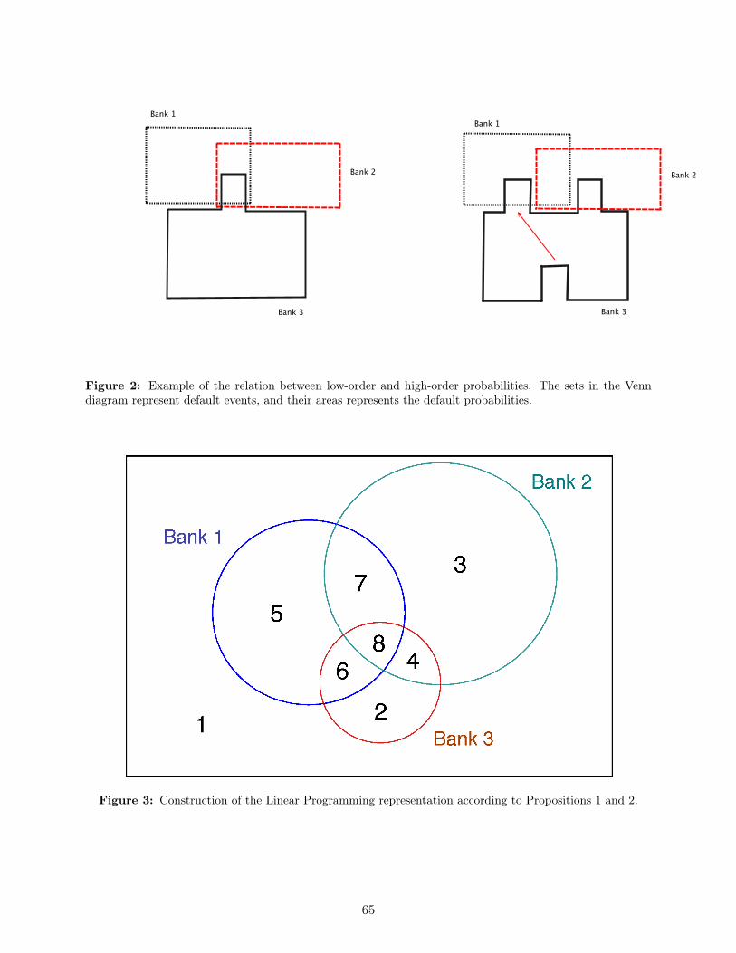
Bank 1

Bank 2

Bank 3

Bank 1

Bank 2

Bank 3

Figure 2: Example of the relation between low-order and high-order probabilities. The sets in the Venndiagram represent default events, and their areas represents the default probabilities.

Figure 3: Construction of the Linear Programming representation according to Propositions 1 and 2.

65

Figure 4: Upper and lower bounds on different systemic events under the assumption of nonnegativeliquidity premia: average monthly probability of at least r banks defaulting, for r = 1, 2, 3, 4. The Figurereports bounds obtained using only information in bond prices (thin lines), only CDS spreads (dotted lines),and all information (shaded area). To reduce noise, I plot a 3 day moving average of each bound. Note thatall lower bounds are 0 for r > 1, and that the CDS-only bounds often coincide with the full informationbounds (that use both bonds and CDSs).

66

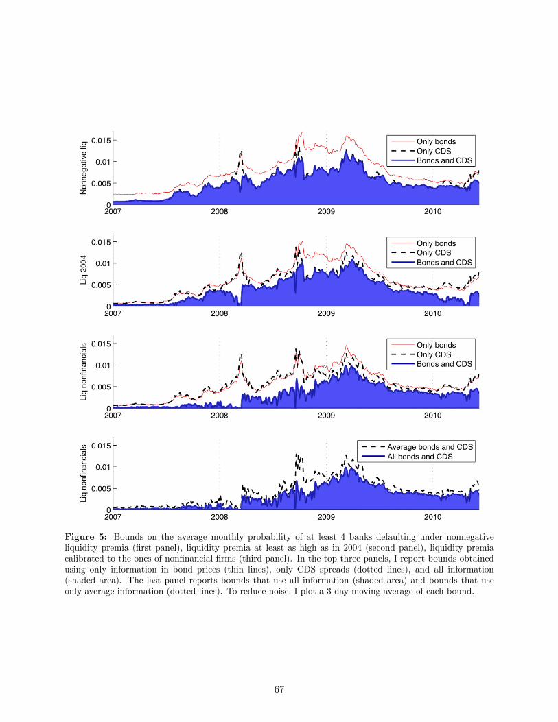
Figure 5: Bounds on the average monthly probability of at least 4 banks defaulting under nonnegativeliquidity premia (first panel), liquidity premia at least as high as in 2004 (second panel), liquidity premiacalibrated to the ones of nonfinancial firms (third panel). In the top three panels, I report bounds obtainedusing only information in bond prices (thin lines), only CDS spreads (dotted lines), and all information(shaded area). The last panel reports bounds that use all information (shaded area) and bounds that useonly average information (dotted lines). To reduce noise, I plot a 3 day moving average of each bound.

67

0.27% 0.19%

0.13%

0.38%

0.33%

0.08% (0 - 0.19%)

0.05% (0 - 0.13%)

0.17% (0.16% - 0.21%)

0.14

% (0

.12%

- 0.

21%)

0.18

% (0

.14%

- 0

.19%

)

0.13% (0.09% - 0.19%)

0.10%

(0.08

% - 0.

13%)

0.08% (0.03% - 0.13%)

0.30% (0.29% - 0.33%)

MS Citi

JPM

Lehman

Merrill0.02% (0% - 0.13%)

Figure 6: Marginal and pairwise average monthly default probabilities for part of the network in the highsystemic risk scenario (max P4) as of 08/06/2008, with the liquidity process calibrated to that of nonfinancialfirms. Nodes report the marginal default probabilities of each banks, edges report pairwise joint defaultprobabilities. The numbers in bold represent the probabilities in the “representative” solution to the bounds,as described in section 3. The numbers in parentheses report the possible range of probabilities across allprobability systems that attain the upper bound on P4.

Jan 2007 Apr 2007 Jul 2007 Oct 2007 Jan 2008 Apr 2008 Jul 2008 Sep 12th 20080

2

4

6

8x 10 3

Mar

gina

l pro

babi

lity

MerrillLehmanCiti

Jan 2007 Apr 2007 Jul 2007 Oct 2007 Jan 2008 Apr 2008 Jul 2008 Sep 12th 20080

1

2

3

4x 10 3

Join

t pro

babi

lity

Merrill & CitiMerrill & LehmanCiti & Lehman

Figure 7: Marginal and pairwise default probabilities for selected banks, in the “representative” solutionto the upper bound for the monthly probability that at least four banks default, under the liquidity processcalibration to nonfinancial firms. To reduce noise, I plot a 3 day moving average of each series.

68

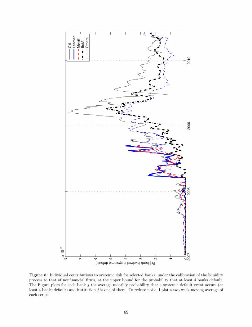
2007

2008

2009

2010

012345678x

103

Pr [ bank involved in systemic default ]

Ci

tiLe

hman

Mer

rill

BofA

Oth

ers

Figure 8: Individual contributions to systemic risk for selected banks, under the calibration of the liquidityprocess to that of nonfinancial firms, at the upper bound for the probability that at least 4 banks default.The Figure plots for each bank j the average monthly probability that a systemic default event occurs (atleast 4 banks default) and institution j is one of them. To reduce noise, I plot a two week moving average ofeach series.

69