FEDERAL RESERVE BANK OF SAN FRANCISCO

WORKING PAPER SERIES

Credit-Fuelled Bubbles

Antonio Doblas-Madrid Michigan State University

Kevin J. Lansing Federal Reserve Bank of San Francisco

March 2016

Working Paper 2016-02 http://www.frbsf.org/economic-research/publications/working-papers/wp2016-02.pdf

Suggested citation:

Doblas-Madrid, Antonio, Kevin J. Lansing. 2016. “Credit-Fuelled Bubbles.” Federal Reserve Bank of San Francisco Working Paper 2016-02. http://www.frbsf.org/economic-research/publications/working-papers/wp2016-02.pdf

The views in this paper are solely the responsibility of the authors and should not be interpreted as reflecting the views of the Federal Reserve Bank of San Francisco or the Board of Governors of the Federal Reserve System.

CREDIT-FUELLED BUBBLES∗

Antonio Doblas-Madrid† Kevin J. Lansing

Abstract

In the context of recent housing busts in the United States and other countries, many

observers have highlighted the role of credit and speculation in fueling unsustainable booms

that lead to crises. Motivated by these observations, we develop a model of credit-fuelled

bubbles in which lenders accept risky assets as collateral. Booming prices allow lenders to

extend more credit, in turn allowing investors to bid prices even higher. Eager to profit from

the boom for as long as possible, asymmetrically informed investors fuel and ride bubbles,

buying overvalued assets in hopes of reselling at a profit to a greater fool. Lucky investors

sell the bubbly asset at peak prices to unlucky ones, who buy in hopes that the bubble will

grow at least a bit longer. In the end, unlucky investors suffer losses, default on their loans,

and lose their collateral to lenders. In our model, tighter monetary and credit policies can

reduce or even eliminate bubbles. These findings are in line with conventional wisdom on

macro prudential regulation, and stand in contrast with those obtained by Galí (2014) in an

overlapping generations context.

JEL Classification: G01, G12

Keywords: Speculative Bubbles, Credit Booms

∗We would like to thank Luis Araujo, Gadi Barlevy, Markus Brunnermeier, Juan Carlos Conesa, Harris Dellas, Hu-berto Ennis, Boyan Jovanovic, Raoul Minetti, Dagfinn Rime, and seminar participants at Norges Bank, Universität Bern, Universitat Autonoma de Barcelona, Michigan State University, Emory University, the University of Miami, the Federal Reserve Bank of Richmond, the Federal Reserve Bank of Chicago, the Kansas Workshop in Economic The-ory, and the Fifth Boston University/Boston Fed Macrofinance Workshop for helpful comments and discussions. All errors are our own.†Corresponding author. Address: Department of Economics 486W Circle Drive 110 Marshall-Adams Hall Michigan

State University East Lansing, MI 48824-1038, USA. Fax: 517.432.1068. Tel: 517.355.7583. Email: doblasma@msu.edu

1

Michigan State University Federal Reserve Bank of San Francisco

1 Introduction

Overinvestment and overspeculation are often important; but they would have far

less serious results were they not conducted with borrowed money.

Irving Fisher, 1933, p.341.

Like Irving Fisher, many economists have highlighted the interplay of credit and specula-

tion as an essential part of booms and crises (Kindleberger and Aliber 2005, Minsky 1986, Borio

and Lowe 2002, Jordà, et al. 2016). Household leverage in many industrial countries increased

dramatically during the mid-2000s. Countries with the largest increases in household debt rel-

ative to income tended to experience the fastest run-ups in house prices over the same period.

The same countries tended to experience the most severe declines in consumption once house

prices started falling (Glick and Lansing 2010, International Monetary Fund 2012).

Within the United States, house prices rose faster in areas where subprime and exotic mort-

gages were more prevalent (Mian and Sufi 2009, Barlevy and Fisher 2010, Pavlov and Wachter

2011, Berkovec, et al. 2012). In a similar vein, the report by the U.S. Financial Crisis Inquiry

Commission (2011) emphasizes the effects of a self-reinforcing feedback loop in which an in-

flux of new homebuyers with access to easy mortgage credit helped fuel an excessive run-up in

house prices, encouraging lenders to ease credit further on the assumption that prices would

continue to rise. While the foregoing studies focus on housing market booms, similar logic ap-

plies to other assets markets, such as stocks, foreign exchange, and derivatives, where margin

trading is common.

Motivated by these observations, we develop a model of credit-fuelled bubbles to analyze

the interplay between lending and speculation. Our starting point is the theory of bubbles pro-

posed by Abreu and Brunnermeier (2003; AB henceforth), and in particular the fully rational

version developed by Doblas-Madrid (2012; DM henceforth). We borrow two key ingredients

from AB. The first is the notion of a bubble as an overreaction to a shock that is at first funda-

mental in nature. The second is the introduction of asymmetric information. In outline, the

model’s structure is as follows. A fundamental shock sets off a boom in asset prices. Initial

price increases are justified by a catch-up to the underlying fundamental v alue. At some time

2

t0 the price becomes just equal to the present value of expected dividends. However, this point

in time is only imperfectly observed, with different investors observing different private signals

about t0. That is, different investors have different information regarding when the fundamen-

tal part of the boom ends and the bubble begins. Since signals are private, investors know their

own signals, but not those of others. Signals order investors along a line from lowest-t0 signal

to highest-t0 signal. This uncertainty is key to generate speculative behavior. Investors know

that if they are early in line, they will sell at peak prices, but they will lose in the crash if they are

late. Nevertheless, as long as price growth is rapid enough to compensate for crash risk, they

are willing to take a chance and ride the bubble. Thus, investors in the model behave like short-

term traders rather than like long-term value investors. Instead of selling as soon as the price

surpasses (their estimation of) fundamental value, they continue to buy the asset in an attempt

to time the market and sell to a greater fool right before the crash.1

Credit plays an essential role in the model because the theory requires that prices expe-

rience a sustained boom instead of a one-time jump. In AB, the sustained boom is due to the

gradual, but accelerating arrival of ’irrationally exuberant’ behavioral agents, whereas in DM, the

lasting boom is made possible by exogenously growing endowments. In both cases, the source

of such growing resources is ultimately unknown. We endogenize this gradual inflow via the in-

teraction between collateralized credit and asset prices. Thus, in addition of being of interest in

its own right, the addition of credit provides a plausible response to a question left unanswered

by previous work.

In our model, each period is subdivided into two stages, an asset market stage where in-

vestors trade assets and a credit market where investors repay old loans and take new ones.

Lenders competitively intermediate between the model economy and the rest of the world,

where they borrow or lend at an exogenous risk-free rate. Investors pledge their shares of the

risky (i.e., bubbly) asset as collateral. Because of limited liability, lenders endogenously adjust

the size of the loans they extend depending on the expected liquidation price of the collateral.

Moreover, in addition to any endogenous lending limits, we assume that lenders face an exoge-

nous upper bound φ on the loan-to-value (LTV) ratio, in which the value of collateral is defined

using the most recent (as opposed to expected future) price. We interpret this as a regulatory

1Barlevy (2015) provides a review of the literature on “greater fool” theories of bubbles.

3

constraint, akin to down payment requirements for home purchases or margin requirement for

stock purchases. Given the difficulty and subjectivity involved in forecasting future prices, such

regulatory limits are in practice defined as a function of observable prices, or appraised values

which typically take recent transactions into account. A link between credit and recent prices

is documented by Dell’Ariccia, et al. (2012) and Goetzmann et al. (2012), who show evidence

that—in US housing markets—recent price appreciation in a given area has a significant posi-

tive impact on subsequent loan approval rates.

While the addition of credit inevitably adds complexity relative to the growing-endowments

model, our model nevertheless remains analytically tractable. Under appropriate parameter

restrictions, the bubble growth rate—generated by a feedback loop between prices and credit—

converges to a constant G. Moreover, we restrict attention to the case in which the LTV cap φ

is low enough that lenders always avoid credit losses when investors default. We refer to this

as a no-risk-shifting condition, under which even in the equilibrium with the biggest bubble,

the hapless late-signal investors who buy at peak prices remain ’above water’ when the price

crashes. These unlucky investors are forced to default on some of their loans when credit tight-

ens in the crash, but these defaults do not saddle lenders with losses because the repossessed

collateral is always valuable enough for full loan repayment. Moreover, since investors are not

’underwater’ they have no incentive to ’walk away’ from their loans in the event of default. This

benchmark analysis gives us a parsimonious extension of DM, to the extent that we can apply

characterization results derived therein with only minor adaptations. The relationship between

bubble growth rate and bubble duration is the same as in the model with endowments. But these

results are supported by with two additional results, one linking the bubble growth rate G to the

degree of leverage φ and one deriving the no-risk-shifting relationship between φ and G and es-

tablishing compatibility between all the conditions needed to sustain equilibrium. Overall, our

results are in line with macro-prudential conventional wisdom regarding interest rates, leverage

and bubbles. The model predicts that looser lending standards (as measured by higher LTV ra-

tios) imply faster growth in the price of the risky asset and therefore longer (and larger) bubbles.

Low interest rates are also conducive to bubbles, for two reasons. First, because the price growth

rate G is decreasing in R, as higher interest payments on borrowed funds slow down the growth

of the funds that investors bring to the asset market. Second, low interest rates make the safe

4

asset unattractive relative to the risky asset. As the G/R ratio increases, so does the size of the

bubble, since investors are willing to risk a bigger crash in exchange for a bigger premium. In

this regard, our results contrast with those of Galí (2014).

The no-risk-shifting condition allows us to isolate the speculative motive for riding of bub-

bles from the risk-shifting motive emphasized by Allen and Gale (2000) and Barlevy (2014),

where investors use borrowed money to bid up prices in excess of expected dividends because

lenders absorb part of the losses in bad states of the world. In our model, as in the growing-

endowments model, investors bear the full costs and benefits of their speculative activity. Thus,

willingness to pay above expected dividends for an asset is purely driven by the prospect of earn-

ing speculative profits, not the possibility of passing losses to third parties if caught in the crash.

Another appealing—and related—feature of the no-risk-shifting analysis is that it is robust to

any specification of lenders’ beliefs about the bubble’s start and bursting times. Since they can-

not lose, lenders offer loans at the exogenous risk-free rate, regardless of their beliefs about t0. In

the context of the recent US housing boom and bust, the no-risk shifting assumption is reminis-

cent of the observation that many mortgage lenders bore little credit risk because of government

guarantees or securitization—although a full analysis along these lines would require analyzing

the beliefs of the securities’ buyers.

In addition to AB, DM and risk-shifting models à la Allen and Gale (2000) and Barlevy (2014),

our work relates to asymmetric information models by Allen, et al. (1993), Conlon (2004, 2015),

and the work by Harrison and Kreps (1978), further extended by Scheinkman and Xiong (2003),

where heterogenous beliefs/overconfidence play a central role. Our model, in addition to asym-

metric information, emphasizes the role of binding constraints in gradually fuelling and riding

bubbles. Finally, our model differs from the well-known ’rational bubbles’ literature pioneered

by Samuelson (1958) and Tirole (1985), and further developed by Martin and Ventura (2012), Galí

(2014), and others. In this strand of literature, bubbles such as fiat money last indefinitely (either

literally or in expectation) and typically have efficiency benefits by helping society overcome a

shortage of stores of value. Our focus, by contrast, is on finite bubbles that are not efficiency

enhancing.

The rest of the paper is organized as follows. Section 2 presents the model. In Section 3,

we define equilibrium and propose a candidate strategy profile. In Section 4, we characterize

5

equilibrium bubble duration in the most tractable, benchmark case. In Section 5, we discuss

our assumptions, results, and possible extensions. In Section 6, we conclude.

2 The Model

Time is discrete and infinite with periods labeled t ∈ {...,−1, 0, 1, 2, ...}. The economy is pop-

ulated by atomistic investors indexed by i ∈ [0, 1] and a continuum of identical lenders. As in

AB and DM, the timeline is split into three phases, a pre-boom phase for t < 0, a boom phase

from t = 0 to the (endogenous) crash period tc, and a post-crash phase for t ≥ tc + 1. The boom

phase may in turn be subdivided into a fundamental part from t = 0 to t = t0 and a bubble from

t0 + 1 to tc. These phases, depicted in Figure 1, describe the evolution of pt, the price of a risky

asset which exists in unit supply and pays dividends {dt}t∈Z. Besides the risky asset, there is a

safe asset which yields an exogenous gross return R and can be turned into consumption at a

one-to-one rate.

In the pre-boom phase t < 0, all agents expect dividends dt to be zero for t ≤ 0 and positive

after period 0. Normalizing the expected value—discounted to time 0—of dividends to 1, the

price pt equals the expected dividend Rt while t < 0. Hence, in the pre-boom phase, the risky

asset is not yet risky, but instead a perfect substitute of the safe asset.

At time 0, an unanticipated shock raises expected dividends. We assume for simplicity that a

single dividend dtpay = FRtpay will be paid at the maturity date tpay > 0. As of time 0, all agents

know that F exceeds 1, but not precisely by how much. There is also uncertainty about tpay,

which is an increasing function of F , so that the greater the fundamental gains from the shock,

the later the payoff. The value of F will be observed at tpay, but we will focus on situations where

F becomes known before then.

A crucial ingredient in our model is the assumption that, due to borrowing constraints, prices

cannot fully adjust to the shock by jumping to the new expected F at t = 0. Instead, the shock

sets off a boom in which higher prices loosen borrowing constraints, allowing investors to bid

prices even higher, and so on. Under certain conditions—which we will derive—the (gross) price

growth rate pt+1/pt generated by this process exceeds R and converges over time to a constant

G > R. Investors can predict the prices that will be observed as long as the boom lasts, but

6

do not know the value of F , and thus do not know how long the price boom will be justified by

fundamentals. Following AB and DM, we denote by t0 ≥ 0 the number of periods it takes for the

price to catch up with the present value of dividends. Specifically, we define

t0 ≡ {t < tc|pt = FRt}.

If prices continue to boom past period t0, a bubble will inflate.2 Bubbly price gains are unjus-

tified by fundamentals and bound to disappear when pt crashes between periods tc and tc + 1.

Following AB, we assume that nature draws t0 from a geometric distribution with pdf

ψ(t0) = (1− λ)λt0 , for t0 = 0, 1, ... (1)

and λ > 0. We also borrow from AB the crucial assumption that investors are asymmetrically in-

formed as follows. At time 0, different investors observe different signals containing information

about t0.3 Specifically, the signal function ν : [0, 1]→ {t0, ..., t0 +N − 1} divides investors into N

types. The signal ν(i) reveals to investor i that the boom may only be justified by fundamentals

up to period ν(i), but not longer. Since investors know that there are N types, investor i infers

that t0 cannot be belowmax{0, ν(i)− (N − 1)} or above ν(i).4 The distribution of t0 conditional

on ν(i) is thus given by

ψ(t0|v(i)) =

ψ(t0)

ψ(max{0,ν(i)−(N−1)})+···+ψ(ν(i)) if max{0, ν(i)− (N − 1)} ≤ t0 ≤ ν(i)

0 otherwise.(2)

Private signals about t0 are equivalent to private signals about F . In fact, signal v(i) reveals that

F ∈ {pt0/Rt0 |max{0, ν(i)− (N − 1)} ≤ t0 ≤ ν(i)}with the probabilities of each possible value of

F given by (2).

Private signals order investors along a line from earliest (i.e., lowest) to latest (i.e., highest)

2In our discrete-time model—as well as in D-M—there has to be a ’coincidence’ for any given price to exactly equalFRt. A more general assumption would be to define t0 as the first period with pt ≥ FRt. However, this complicatesformulae substantially without yielding additional insight.

3In AB and D-M, signals arrive overN periods of time, starting at t0. Our assumption that all signals arrive at time0 simplifies the exposition without affecting results.

4Themax{0, ·} operator captures the fact that, in the special case with t0 < N − 1, types with ν(i) < N − 1 knowthat they cannot be last in line, since ν(i) − (N − 1) < 0. For those types, the support of t0 conditional on ν(i) is{0, ..., ν(i)} instead of {ν(i)− (N − 1), ..., ν(i)}.

7

signal, but they do not know their relative order in the line. Importantly, all investors—including

those late in the line—assign positive probability to the event that they could be early.5 As we will

see, given the speed at which the bubble grows and the probability of a crash, investors will ride

and fuel bubbles as long as prospective speculative gains in the event of being an early-signal

investor outweigh the risky of losses in the event of being a late-signal investors. Thus, as in AB

and DM, we model a bubble as a situation in which markets overreact to a fundamental shock,

with the overreaction arising as the equilibrium of a market timing game played by investors.

Compared to investors, lenders are relatively passive. Since we focus on equilibria without risk-

shifting, we do not need to make assumptions about whether they observe any signals.

The boom continues as long as all types continue to invest in it, and ends as soon as one type

exits the market anticipating a crash. To fix ideas, suppose that type-ν(i) investors plan to ride

the bubble for τ∗ ≥ 0 periods and then sell at ν(i) + τ∗. (We will later construct equilibria in

which this is the case.) While t < t0 + τ∗, all types of investors are fully invested in the bubble.

The crash arrives at tc = t0 + τ∗ when investors of type ν(i) = t0 exit the market. Their sales

affect the price, revealing to others that t = tc and that t0 = tc − τ∗.6 The boom concludes

with investors of type ν(i) = t0 selling at the peak and all other types finding themselves in the

position of the greater fool. Post-crash, the value of t0 is common knowledge, and the risky asset

trades at fundamental value pt = E[F |t0]Rt until the payoff date tpay, falling to zero afterwards.

Keeping this sketch of the model in mind, we now proceed to a full description of the envi-

ronment.

2.1 Preferences

Investors are risk neutral, and may be hit by preference shocks à la Diamond and Dybvig (1983),

which induce an urgent need to consume. Specifically, every period a randomly chosen fraction

θ ∈ [0, 1] of investors are hit by a shock that makes them impatient by setting their discount

factor δi,t to 0, while the remaining mass 1 − θ are patient and have discount factor δi,t = 1/R.

5This specification of signals is simply a discretized version of that in AB. Moreover, it resembles the timing devisedby Moinas and Pouget (2012), who conduct experiments in which participants are uncertain about the order in whichthey move relative to each other.

6As we will shortly see, the trading protocol is such that agents submit orders first, and observe the price second.Thus, unlike in a Walrasian setting, buyers get stuck with the bubble at tc because they cannot change their ordersafter observing the price.

8

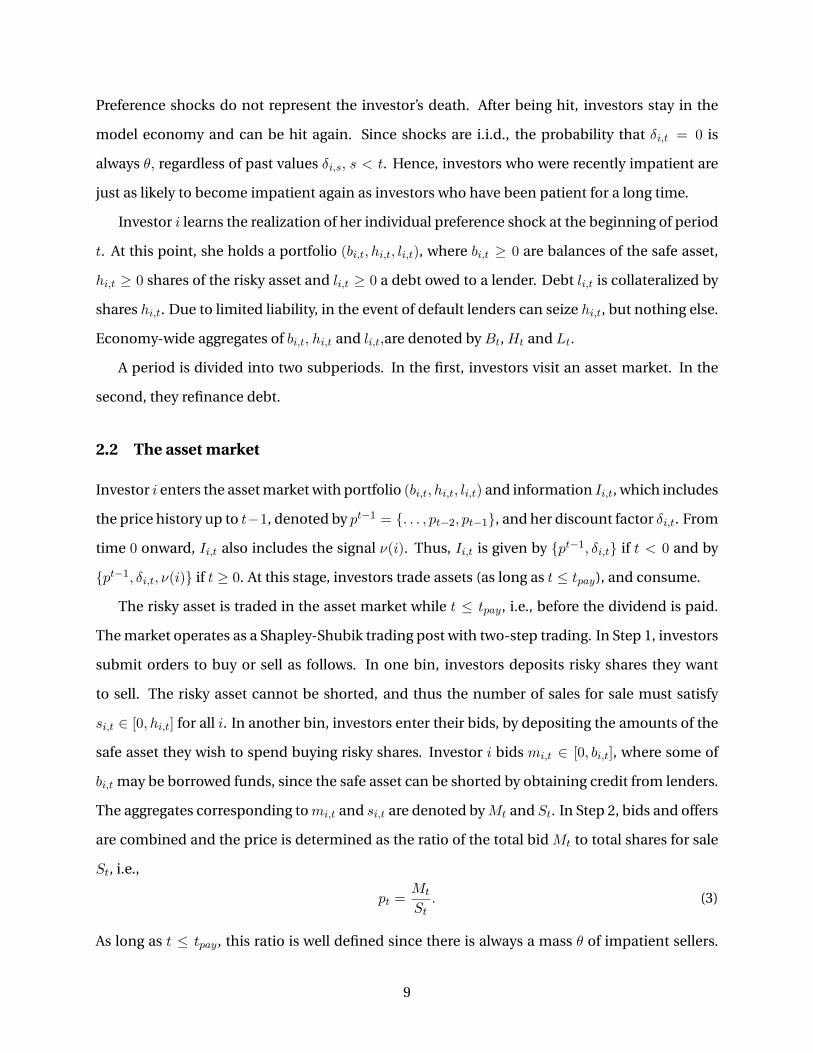
Preference shocks do not represent the investor’s death. After being hit, investors stay in the

model economy and can be hit again. Since shocks are i.i.d., the probability that δi,t = 0 is

always θ, regardless of past values δi,s, s < t. Hence, investors who were recently impatient are

just as likely to become impatient again as investors who have been patient for a long time.

Investor i learns the realization of her individual preference shock at the beginning of period

t. At this point, she holds a portfolio (bi,t, hi,t, li,t), where bi,t ≥ 0 are balances of the safe asset,

hi,t ≥ 0 shares of the risky asset and li,t ≥ 0 a debt owed to a lender. Debt li,t is collateralized by

shares hi,t. Due to limited liability, in the event of default lenders can seize hi,t, but nothing else.

Economy-wide aggregates of bi,t, hi,t and li,t,are denoted by Bt, Ht and Lt.

A period is divided into two subperiods. In the first, investors visit an asset market. In the

second, they refinance debt.

2.2 The asset market

Investor i enters the asset market with portfolio (bi,t, hi,t, li,t) and information Ii,t, which includes

the price history up to t−1, denoted by pt−1 = {. . . , pt−2, pt−1}, and her discount factor δi,t. From

time 0 onward, Ii,t also includes the signal ν(i). Thus, Ii,t is given by {pt−1, δi,t} if t < 0 and by

{pt−1, δi,t, ν(i)} if t ≥ 0. At this stage, investors trade assets (as long as t ≤ tpay), and consume.

The risky asset is traded in the asset market while t ≤ tpay, i.e., before the dividend is paid.

The market operates as a Shapley-Shubik trading post with two-step trading. In Step 1, investors

submit orders to buy or sell as follows. In one bin, investors deposits risky shares they want

to sell. The risky asset cannot be shorted, and thus the number of sales for sale must satisfy

si,t ∈ [0, hi,t] for all i. In another bin, investors enter their bids, by depositing the amounts of the

safe asset they wish to spend buying risky shares. Investor i bids mi,t ∈ [0, bi,t], where some of

bi,t may be borrowed funds, since the safe asset can be shorted by obtaining credit from lenders.

The aggregates corresponding tomi,t and si,t are denoted byMt and St. In Step 2, bids and offers

are combined and the price is determined as the ratio of the total bid Mt to total shares for sale

St, i.e.,

pt =Mt

St. (3)

As long as t ≤ tpay, this ratio is well defined since there is always a mass θ of impatient sellers.

9

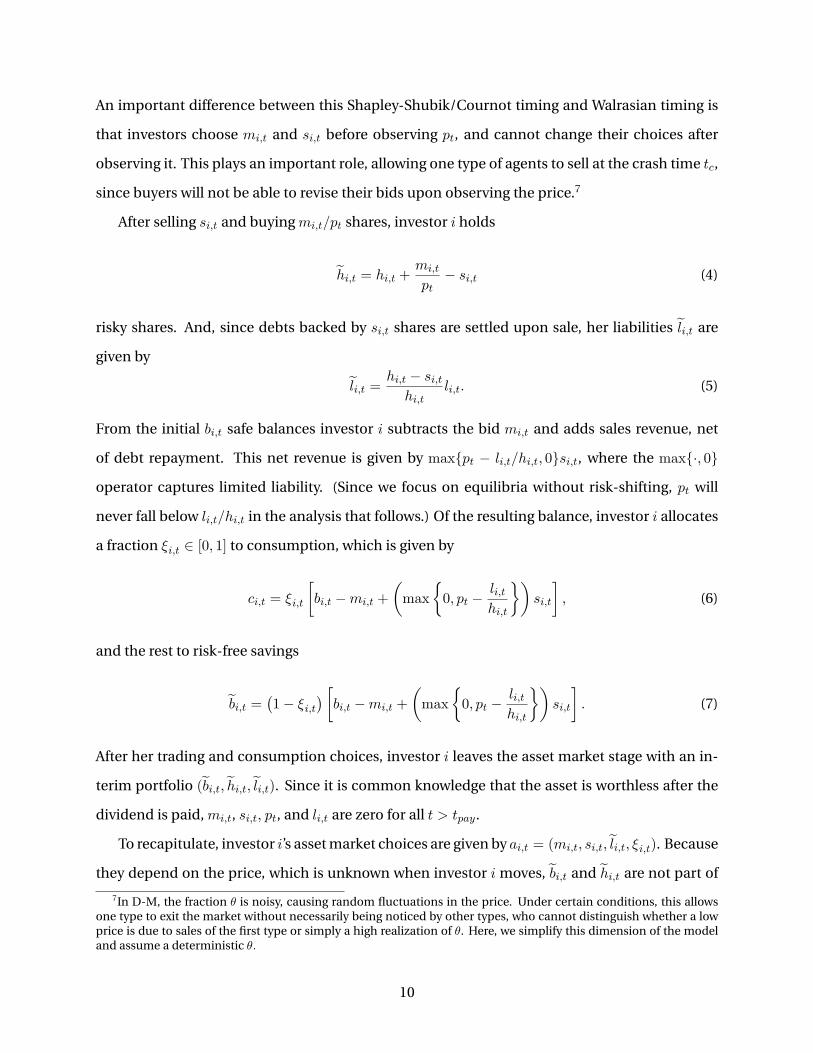
An important difference between this Shapley-Shubik/Cournot timing and Walrasian timing is

that investors choose mi,t and si,t before observing pt, and cannot change their choices after

observing it. This plays an important role, allowing one type of agents to sell at the crash time tc,

since buyers will not be able to revise their bids upon observing the price.7

After selling si,t and buying mi,t/pt shares, investor i holds

hi,t = hi,t +mi,t

pt− si,t (4)

risky shares. And, since debts backed by si,t shares are settled upon sale, her liabilities li,t are

given by

li,t =hi,t − si,thi,t

li,t. (5)

From the initial bi,t safe balances investor i subtracts the bid mi,t and adds sales revenue, net

of debt repayment. This net revenue is given by max{pt − li,t/hi,t, 0}si,t, where the max{·, 0}

operator captures limited liability. (Since we focus on equilibria without risk-shifting, pt will

never fall below li,t/hi,t in the analysis that follows.) Of the resulting balance, investor i allocates

a fraction ξi,t ∈ [0, 1] to consumption, which is given by

ci,t = ξi,t

[bi,t −mi,t +

(max

{0, pt −

li,thi,t

})si,t

], (6)

and the rest to risk-free savings

bi,t =(1− ξi,t

) [bi,t −mi,t +

(max

{0, pt −

li,thi,t

})si,t

]. (7)

After her trading and consumption choices, investor i leaves the asset market stage with an in-

terim portfolio (bi,t, hi,t, li,t). Since it is common knowledge that the asset is worthless after the

dividend is paid, mi,t, si,t, pt, and li,t are zero for all t > tpay.

To recapitulate, investor i’s asset market choices are given by ai,t = (mi,t, si,t, li,t, ξi,t). Because

they depend on the price, which is unknown when investor i moves, bi,t and hi,t are not part of

7In D-M, the fraction θ is noisy, causing random fluctuations in the price. Under certain conditions, this allowsone type to exit the market without necessarily being noticed by other types, who cannot distinguish whether a lowprice is due to sales of the first type or simply a high realization of θ. Here, we simplify this dimension of the modeland assume a deterministic θ.

10

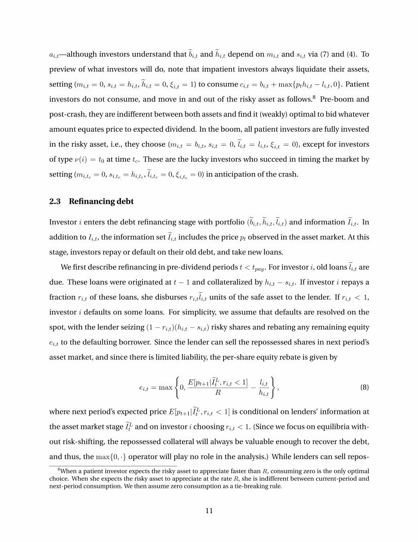
ai,t—although investors understand that bi,t and hi,t depend on mi,t and si,t via (7) and (4). To

preview of what investors will do, note that impatient investors always liquidate their assets,

setting (mi,t = 0, si,t = hi,t, hi,t = 0, ξi,t = 1) to consume ci,t = bi,t +max{pthi,t − li,t, 0}. Patient

investors do not consume, and move in and out of the risky asset as follows.8 Pre-boom and

post-crash, they are indifferent between both assets and find it (weakly) optimal to bid whatever

amount equates price to expected dividend. In the boom, all patient investors are fully invested

in the risky asset, i.e., they choose (mi,t = bi,t, si,t = 0, li,t = li,t, ξi,t = 0), except for investors

of type ν(i) = t0 at time tc. These are the lucky investors who succeed in timing the market by

setting (mi,tc = 0, si,tc = hi,tc , li,tc = 0, ξi,tc = 0) in anticipation of the crash.

2.3 Refinancing debt

Investor i enters the debt refinancing stage with portfolio (bi,t, hi,t, li,t) and information Ii,t. In

addition to Ii,t, the information set Ii,t includes the price pt observed in the asset market. At this

stage, investors repay or default on their old debt, and take new loans.

We first describe refinancing in pre-dividend periods t < tpay. For investor i, old loans li,t are

due. These loans were originated at t − 1 and collateralized by hi,t − si,t. If investor i repays a

fraction ri,t of these loans, she disburses ri,t li,t units of the safe asset to the lender. If ri,t < 1,

investor i defaults on some loans. For simplicity, we assume that defaults are resolved on the

spot, with the lender seizing (1 − ri,t)(hi,t − si,t) risky shares and rebating any remaining equity

ei,t to the defaulting borrower. Since the lender can sell the repossessed shares in next period’s

asset market, and since there is limited liability, the per-share equity rebate is given by

ei,t = max

{0,E[pt+1|ILt , ri,t < 1]

R− li,thi,t

}, (8)

where next period’s expected price E[pt+1|ILt , ri,t < 1] is conditional on lenders’ information at

the asset market stage ILt and on investor i choosing ri,t < 1. (Since we focus on equilibria with-

out risk-shifting, the repossessed collateral will always be valuable enough to recover the debt,

and thus, the max{0, ·} operator will play no role in the analysis.) While lenders can sell repos-

8When a patient investor expects the risky asset to appreciate faster than R, consuming zero is the only optimalchoice. When she expects the risky asset to appreciate at the rate R, she is indifferent between current-period andnext-period consumption. We then assume zero consumption as a tie-breaking rule.

11

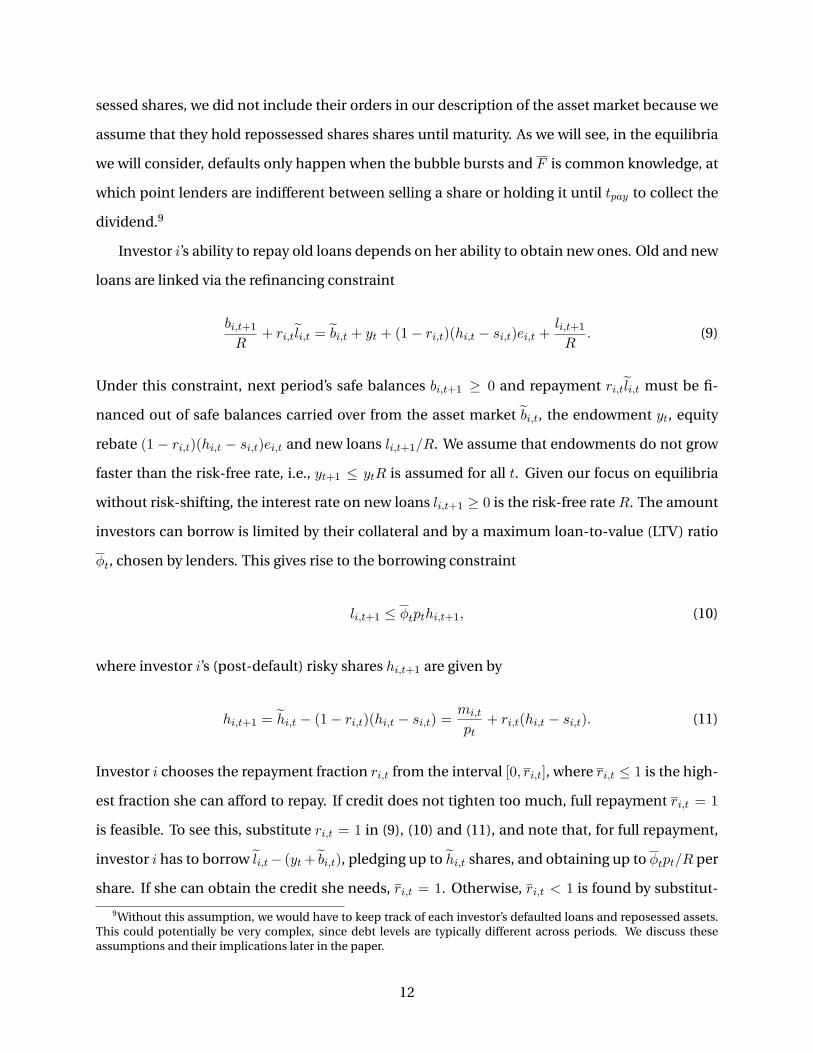
sessed shares, we did not include their orders in our description of the asset market because we

assume that they hold repossessed shares shares until maturity. As we will see, in the equilibria

we will consider, defaults only happen when the bubble bursts and F is common knowledge, at

which point lenders are indifferent between selling a share or holding it until tpay to collect the

dividend.9

Investor i’s ability to repay old loans depends on her ability to obtain new ones. Old and new

loans are linked via the refinancing constraint

bi,t+1R

+ ri,t li,t = bi,t + yt + (1− ri,t)(hi,t − si,t)ei,t +li,t+1R

. (9)

Under this constraint, next period’s safe balances bi,t+1 ≥ 0 and repayment ri,t li,t must be fi-

nanced out of safe balances carried over from the asset market bi,t, the endowment yt, equity

rebate (1 − ri,t)(hi,t − si,t)ei,t and new loans li,t+1/R. We assume that endowments do not grow

faster than the risk-free rate, i.e., yt+1 ≤ ytR is assumed for all t. Given our focus on equilibria

without risk-shifting, the interest rate on new loans li,t+1 ≥ 0 is the risk-free rate R. The amount

investors can borrow is limited by their collateral and by a maximum loan-to-value (LTV) ratio

φt, chosen by lenders. This gives rise to the borrowing constraint

li,t+1 ≤ φtpthi,t+1, (10)

where investor i’s (post-default) risky shares hi,t+1 are given by

hi,t+1 = hi,t − (1− ri,t)(hi,t − si,t) =mi,t

pt+ ri,t(hi,t − si,t). (11)

Investor i chooses the repayment fraction ri,t from the interval [0, ri,t], where ri,t ≤ 1 is the high-

est fraction she can afford to repay. If credit does not tighten too much, full repayment ri,t = 1

is feasible. To see this, substitute ri,t = 1 in (9), (10) and (11), and note that, for full repayment,

investor i has to borrow li,t− (yt+ bi,t), pledging up to hi,t shares, and obtaining up to φtpt/R per

share. If she can obtain the credit she needs, ri,t = 1. Otherwise, ri,t < 1 is found by substitut-

9Without this assumption, we would have to keep track of each investor’s defaulted loans and reposessed assets.This could potentially be very complex, since debt levels are typically different across periods. We discuss theseassumptions and their implications later in the paper.

12

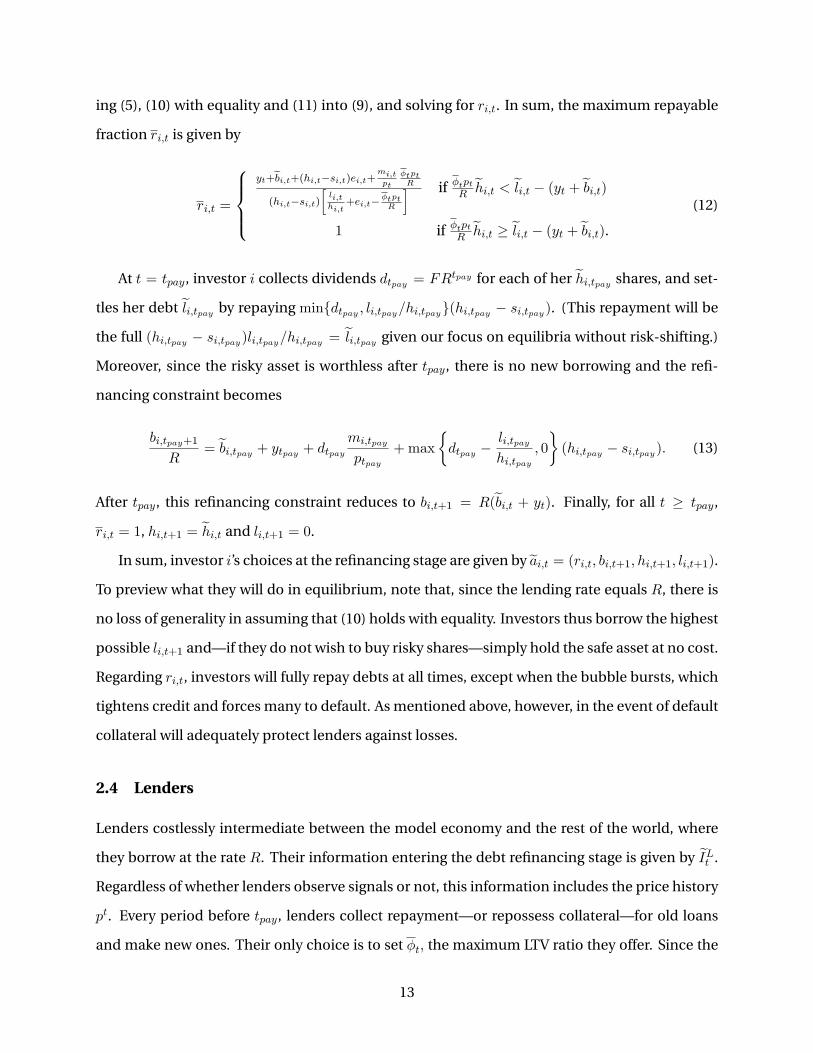
ing (5), (10) with equality and (11) into (9), and solving for ri,t. In sum, the maximum repayable

fraction ri,t is given by

ri,t =

yt+bi,t+(hi,t−si,t)ei,t+

mi,tpt

φtptR

(hi,t−si,t)[li,thi,t

+ei,t−φtptR

] if φtptR hi,t < li,t − (yt + bi,t)

1 if φtptR hi,t ≥ li,t − (yt + bi,t).(12)

At t = tpay, investor i collects dividends dtpay = FRtpay for each of her hi,tpay shares, and set-

tles her debt li,tpay by repaying min{dtpay , li,tpay/hi,tpay}(hi,tpay − si,tpay). (This repayment will be

the full (hi,tpay − si,tpay)li,tpay/hi,tpay = li,tpay given our focus on equilibria without risk-shifting.)

Moreover, since the risky asset is worthless after tpay, there is no new borrowing and the refi-

nancing constraint becomes

bi,tpay+1

R= bi,tpay + ytpay + dtpay

mi,tpay

ptpay+max

{dtpay −

li,tpayhi,tpay

, 0

}(hi,tpay − si,tpay). (13)

After tpay, this refinancing constraint reduces to bi,t+1 = R(bi,t + yt). Finally, for all t ≥ tpay,

ri,t = 1, hi,t+1 = hi,t and li,t+1 = 0.

In sum, investor i’s choices at the refinancing stage are given by ai,t = (ri,t, bi,t+1, hi,t+1, li,t+1).

To preview what they will do in equilibrium, note that, since the lending rate equals R, there is

no loss of generality in assuming that (10) holds with equality. Investors thus borrow the highest

possible li,t+1 and—if they do not wish to buy risky shares—simply hold the safe asset at no cost.

Regarding ri,t, investors will fully repay debts at all times, except when the bubble bursts, which

tightens credit and forces many to default. As mentioned above, however, in the event of default

collateral will adequately protect lenders against losses.

2.4 Lenders

Lenders costlessly intermediate between the model economy and the rest of the world, where

they borrow at the rate R. Their information entering the debt refinancing stage is given by ILt .

Regardless of whether lenders observe signals or not, this information includes the price history

pt. Every period before tpay, lenders collect repayment—or repossess collateral—for old loans

and make new ones. Their only choice is to set φt, the maximum LTV ratio they offer. Since the

13

risky asset is worthless after tpay, φt = 0 for all t ≥ tpay.

The highest LTV offered φt depends on repayment expectations, but is also subject to an

exogenous upper bound

φt ≤ φ. (14)

As discussed in the introduction, we interpret this as a regulatory constraint, akin to a down

payment requirement for a mortgage, or margin requirements for stock traders. Our assump-

tion is motivated by the observation that, lending caps are in practice expressed as a function

of current prices, rather than expected future prices, because the former can be observed or

appraised more easily and objectively. Although we do not model regulators, this kind of lever-

age constraint is often part of banking, or macro-prudential regulations, aimed at reducing the

frequency and severity of financial crises.

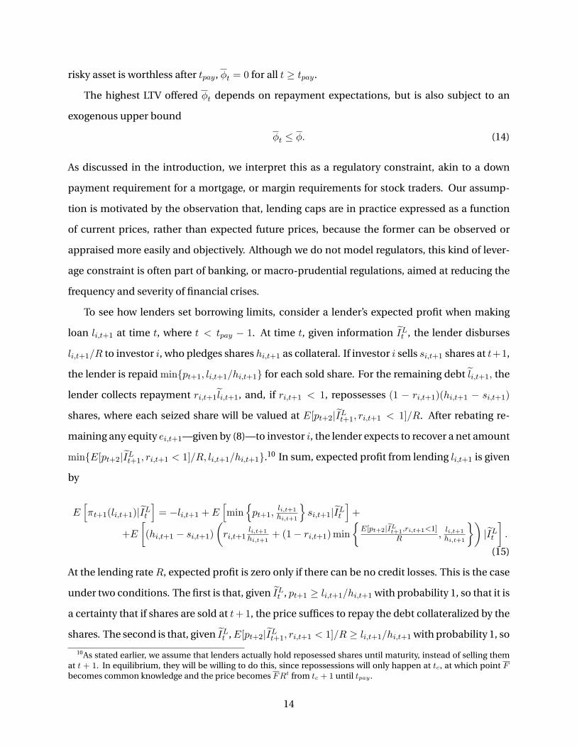
To see how lenders set borrowing limits, consider a lender’s expected profit when making

loan li,t+1 at time t, where t < tpay − 1. At time t, given information ILt , the lender disburses

li,t+1/R to investor i, who pledges shares hi,t+1 as collateral. If investor i sells si,t+1 shares at t+1,

the lender is repaidmin{pt+1, li,t+1/hi,t+1} for each sold share. For the remaining debt li,t+1, the

lender collects repayment ri,t+1 li,t+1, and, if ri,t+1 < 1, repossesses (1 − ri,t+1)(hi,t+1 − si,t+1)

shares, where each seized share will be valued at E[pt+2|ILt+1, ri,t+1 < 1]/R. After rebating re-

maining any equity ei,t+1—given by (8)—to investor i, the lender expects to recover a net amount

min{E[pt+2|ILt+1, ri,t+1 < 1]/R, li,t+1/hi,t+1}.10 In sum, expected profit from lending li,t+1 is given

by

E[πt+1(li,t+1)|ILt

]= −li,t+1 + E

[min

{pt+1,

li,t+1hi,t+1

}si,t+1|ILt

]+

+E

[(hi,t+1 − si,t+1)

(ri,t+1

li,t+1hi,t+1

+ (1− ri,t+1)min{E[pt+2|ILt+1,ri,t+1<1]

R ,li,t+1hi,t+1

})|ILt].

(15)

At the lending rateR, expected profit is zero only if there can be no credit losses. This is the case

under two conditions. The first is that, given ILt , pt+1 ≥ li,t+1/hi,t+1 with probability 1, so that it is

a certainty that if shares are sold at t+1, the price suffices to repay the debt collateralized by the

shares. The second is that, given ILt ,E[pt+2|ILt+1, ri,t+1 < 1]/R ≥ li,t+1/hi,t+1 with probability 1, so

10As stated earlier, we assume that lenders actually hold reposessed shares until maturity, instead of selling themat t + 1. In equilibrium, they will be willing to do this, since repossessions will only happen at tc, at which point Fbecomes common knowledge and the price becomes FRt from tc + 1 until tpay.

14

that if shares are not sold and the borrower defaults, it is certain that the collateral will suffice to

recover the debt. Given the borrowing constraint li,t+1/hi,t+1 ≤ φtpt, to maximize profit—which

absent risk-shifting means earning zero profit—the LTV cap φt must satisfy

Pr

[φt ≤ min

{pt+1pt

,E[pt+2|ILt+1, ri,t+1 < 1]

Rpt

}|ILt

]= 1. (16)

Absence of risk-shifing will depend crucially on the upper bound φ, which will limit price

growth in the boom. If φ is below a threshold—which we will derive—lenders will avoid credit

losses even on loans made right before the crash, at tc − 1. Most borrowers will spend these

borrowed funds buying risky shares at time tc, only to realize as soon as they observe the price

ptc that the bubble has burst. Since ptc+1 will fall to equal fundamental value, lenders will choose

φtc < φ, i.e., (14) will not bind at time tc. From period tc + 1 until tpay − 1, (14) will bind again.

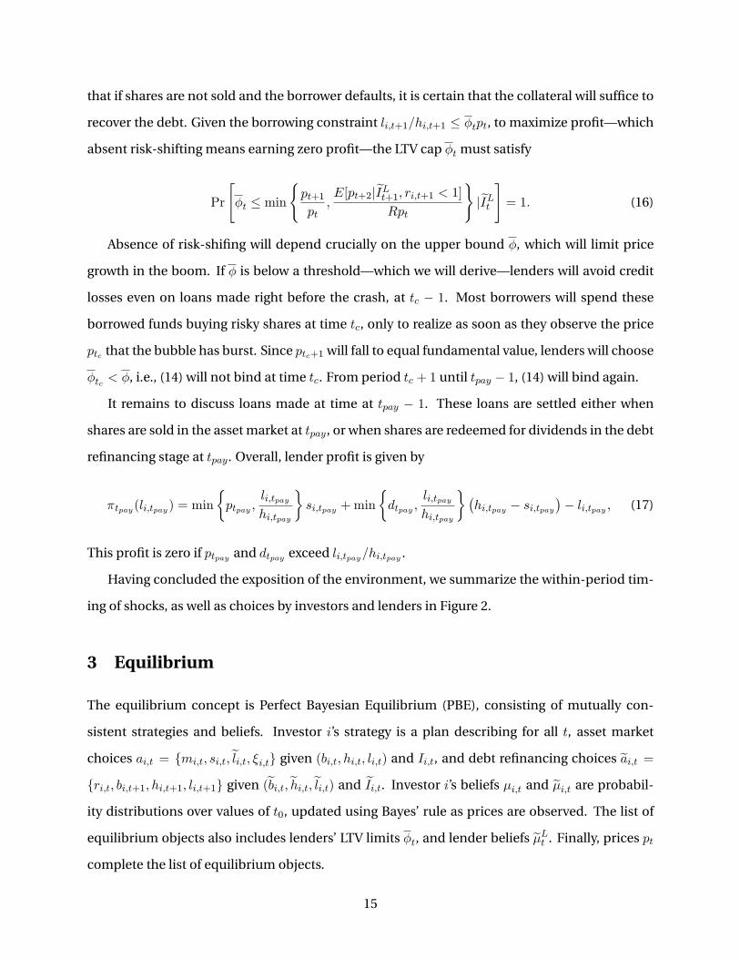
It remains to discuss loans made at time at tpay − 1. These loans are settled either when

shares are sold in the asset market at tpay, or when shares are redeemed for dividends in the debt

refinancing stage at tpay. Overall, lender profit is given by

πtpay(li,tpay) = min

{ptpay ,

li,tpayhi,tpay

}si,tpay +min

{dtpay ,

li,tpayhi,tpay

}(hi,tpay − si,tpay

)− li,tpay , (17)

This profit is zero if ptpay and dtpay exceed li,tpay/hi,tpay .

Having concluded the exposition of the environment, we summarize the within-period tim-

ing of shocks, as well as choices by investors and lenders in Figure 2.

3 Equilibrium

The equilibrium concept is Perfect Bayesian Equilibrium (PBE), consisting of mutually con-

sistent strategies and beliefs. Investor i’s strategy is a plan describing for all t, asset market

choices ai,t = {mi,t, si,t, li,t, ξi,t} given (bi,t, hi,t, li,t) and Ii,t, and debt refinancing choices ai,t =

{ri,t, bi,t+1, hi,t+1, li,t+1} given (bi,t, hi,t, li,t) and Ii,t. Investor i’s beliefs µi,t and µi,t are probabil-

ity distributions over values of t0, updated using Bayes’ rule as prices are observed. The list of

equilibrium objects also includes lenders’ LTV limits φt, and lender beliefs µLt . Finally, prices pt

complete the list of equilibrium objects.

15

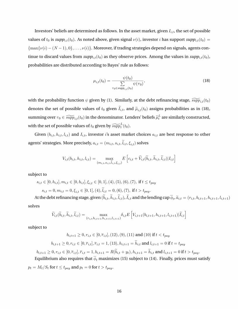
Investors’ beliefs are determined as follows. In the asset market, given Ii,t, the set of possible

values of t0 is suppi,t(t0). As noted above, given signal ν(i), investor i has support suppi,t(t0) =

{max{ν(i)− (N − 1), 0}, . . . , ν(i)}. Moreover, if trading strategies depend on signals, agents con-

tinue to discard values from suppi,t(t0) as they observe prices. Among the values in suppi,t(t0),

probabilities are distributed according to Bayes’ rule as follows:

µi,t(t0) =ψ(t0)∑

τ0∈suppi,t(t0)ψ(τ0)

, (18)

with the probability function ψ given by (1). Similarly, at the debt refinancing stage, suppi,t(t0)

denotes the set of possible values of t0 given Ii,t, and µi,t(t0) assigns probabilities as in (18),

summing over τ0 ∈ suppi,t(t0) in the denominator. Lenders’ beliefs µLt are similarly constructed,

with the set of possible values of t0 given by suppLt (t0).

Given (bi,t, hi,t, li,t) and Ii,t, investor i’s asset market choices ai,t are best response to other

agents’ strategies. More precisely, ai,t = (mi,t, si,t, li,t, ξi,t) solves

Vi,t(bi,t, hi,t, li,t) = max(mi,t,si,t,li,t,ξi,t)

E[ci,t + Vi,t(bi,t, hi,t, li,t)|Ii,t

]

subject to

si,t ∈ [0, hi,t],mi,t ∈ [0, bi,t], ξi,t ∈ [0, 1], (4), (5), (6), (7), if t ≤ tpay

si,t = 0,mi,t = 0, ξi,t ∈ [0, 1], (4), li,t = 0, (6), (7), if t > tpay.

At the debt refinancing stage, given (bi,t, hi,t, li,t), Ii,t and the lending capφt, ai,t = (ri,t, bi,t+1, hi,t+1, li,t+1)

solves

Vi,t(bi,t, hi,t, li,t) = max(ri,t,bi,t+1,hi,t+1,li,t+1)

δi,tE[Vi,t+1(bi,t+1, hi,t+1, li,t+1)|Ii,t

]subject to

bi,t+1 ≥ 0, ri,t ∈ [0, ri,t], (12), (9), (11) and (10) if t < tpay

bi,t+1 ≥ 0, ri,t ∈ [0, ri,t], ri,t = 1, (13), hi,t+1 = hi,t and li,t+1 = 0 if t = tpay

bi,t+1 ≥ 0, ri,t ∈ [0, ri,t], ri,t = 1, bi,t+1 = R(bi,t + yt), hi,t+1 = hi,t and li,t+1 = 0 if t > tpay.

Equilibrium also requires that φt maximizes (15) subject to (14). Finally, prices must satisfy

pt =Mt/St for t ≤ tpay and pt = 0 for t > tpay.

16

4 Bubbles without risk shifting

We focus on situations in which the LTV cap φ is low enough to avoid risk-shifting. In this case,

even the largest bubble and debt that can arise in equilibrium are low enough to keep borrow-

ers ’above water’ when the bubble bursts. Since the unlucky investors who buy at time tc have

positive equity after the crash, the collateral seized by lenders in the event of default is valuable

enough to recover principal and interest on outstanding loans. Absence of credit losses allows

us to greatly simplify the credit market. Since loans are repaid for any t0, the probabilites that

lenders assign to different values of t0 are irrelevant, and the competitive interest rate function is

a constantR for all LTV ratios offered. Investors’ debt refinancing plans are also simple—borrow

as much as possible, i.e., li,t+1 = φtpthi,t+1 at all times. The price dynamics that arise in this

case converge to those in the growing-endowment environment of DM, allowing us to apply

bubble characterization results subject to only minor modifications. Our model thus provides a

parsimonious, credit-based justification for the growth in investable funds that is exogenous in

previous work.

4.1 Strategies

To find equilibria, we follow a guess-and-verify procedure. We conjecture a strategy profile for

investors, and lending caps for lenders, and then verify that the conjectured plans are optimal

given the beliefs and prices that they imply.

We begin by conjecturing that lenders set the following LTV bounds. For all t < tpay, except

for t = tc, they offer the highest allowed φt = φ. At time tc, after seeing the price ptc , it becomes

common knowledge that ptc+1 = FRtc+1, where F = pt0/Rt0 is also common knowledge at this

point known. If φptc > FRtc , lending φptc against the value of a share worth FRtc would result in

losses. In that case, they adjust the maximum LTV ratio φtc downward to less than φ. Once the

price crashes at tc+1, φtc+1 increases to φ, although loans will be smaller than at time tc because

of lower collateral values. Finally, φtpay = 0 since the price pt is zero for all t > tpay. In sum,

17

φt =

φ if t 6= tc and t < tpay

min{φ, FRtc/ptc} if t = tc

0 if t ≥ tpay.

(19)

Let us next turn to investors. Impatient investors liquidate all their assets to consume ci,t =

bi,t + pthi,t − li,t and leave the asset market with (bi,t, hi,t, li,t) = (0, 0, 0). At the debt refinanc-

ing stage, they simply collect endowments. Patient investors, as in AB and DM, follow trigger

strategies. Type-ν(i) investors plan to ride the bubble for τ∗ periods and sell at time ν(i) + τ∗,

unless the bubble bursts before then. We also assume that patient investors do not consume,

and that pre-boom and post-crash, they simply bid the necessary amount to keep price equal to

fundamental value. More precisely, the strategy of investor i {ai,t, ai,t} is as follows:

(i) If impatient, δi,t = 0:

ai,t = (mi,t, si,t, li,t, ξi,t) =

(0, hi,t, 0, 1) if t ≤ tpay.

(0, 0, 0, 1) if t > tpay.(20a)

ai,t = (ri,t, bi,t+1, hi,t+1, li,t+1) = (1, ytR, 0, 0). (20b)

(ii) If patient, δi,t = 1/R, asset market choices are given by ai,t = (ri,t, bi,t+1, hi,t+1, li,t+1)

ai,t = (mi,t, si,t, li,t, ξi,t) =

(θ1−θ

Rt

Btbit, 0, li,t, 0

)if t < 0

(bi,t + yt, 0, li,t, 0) if 0 ≤ t < min{ν(i) + τ∗, tc + 1}

(0, hi,t, 0, 0) if t = ν(i) + τ∗ < tc + 1(θ1−θ

FRt

Btbit, 0, li,t, 0

)if tc + 1 ≤ t ≤ tpay

(0, 0, 0, 0) if t > tpay

(20c)

And debt refinancing choices ai,t = (ri,t, bi,t+1, hi,t+1, li,t+1) are given by

hi,t+1 and li,t+1 are respectively given by hi,t − (1 − ri,t)(hi,t − si,t) and φtpthi,t+1, for all t,

18

where the repayment fraction ri,t is given by

ri,t =

1 if t 6= tc

ηri,tc if t = tc,(4)

and η ∈ (0, 1) is small enough to ensure that agents have enough funds to bid prices up to

expected dividend after tc. Safe savings bi,t+1 are given by

bi,t+1 =

R[bi,t + yt + (1− ri,t)(hi,t − si,t)ei,t − ri,t li,t

]+ li,t+1 if t < tpay

R(bi,t + yt + dthi,t − li,t) if t = tpay

R(bi,t + yt) if t > tpay.

(5)

And for all t,

hi,t+1 = hi,t − (1− ri,t)(hi,t − si,t) (6)

and

li,t+1 = φtpthi,t+1. (7)

Given strategies, lender and investor beliefs evolve as follows. Lenders—regardless of whether

they observe signals—know that t0 cannot be negative, and that the crash will happen τ∗ periods

after t0. If they only observe prices, they can infer that the support of t0 is infinite, with no upper

bound, and a lower bound given by max{0, t − τ∗ + 1}. Once they observe the crash, they learn

that t0 = tc − τ∗. In sum,

suppLt (t0|pt) =

{τ0 ∈ Z|τ0 ≥ max{0, t− τ∗ + 1}} if 0 ≤ t < tc

{tc − τ∗} if t ≥ tc.(21)

The actual support of lenders may be more refined than this, if they observe signals. However,

in equilibria without risk shifting, this will suffice.

Investors, in addition to observing whether the bubble has burst, also observe signals. Before

the crash, investors know that t0 must be nonnegative and, since the crash has not happened as

of time t, greater than t− τ∗. The signal v(i) allows investor i to narrow the support of t0 between

19

a lower bound ν(i) − (N − 1) and an upper bound ν(i). In sum, given strategies, the support of

t0 for investor i at the debt refinancing stage of period t is given by

suppi,t(t0) =

τ0 ∈ {max{0, t− τ∗ + 1, ν(i)− (N − 1)}, ..., ν(i)} if 0 ≤ t < tc

{tc − τ∗} if t ≥ tc.(22)

To understand this expression, it is most illustrative to consider an investor i with ν(i) ≥ N − 1.

Once she observes the price pν(i)−(N−1)+τ∗ , she learns that t0 = ν(i)−(N−1) if the bubble bursts,

or that t0 > ν(i)− (N − 1) otherwise. Every period after that, the bubble either bursts, revealing

the value of t0, or continues, in which case she drops the lowest value from the support of t0.

As the bubble continues and values are discarded, the probability that the crash happens in the

next period increases. In fact, if t0 happens to be ν(i), investor i learns the true value of t0 when

she sees that the bubble does not burst at t = ν(i) − 1 + τ∗, which allows her to rule out the

possibility that t0 = ν(i)− 1 and be certain that t0 = ν(i).

Finally, since no new prices or signals are observed between the debt refinancing stage of

period t and the asset market stage of period t + 1, the support of t0 at the asset market stage is

suppi,0(t0) = {0, 1, 2, ...} for t = 0, and for t ≥ 1,

suppi,t+1(t0) = suppi,t(t0). (23)

4.2 Equilibrium boom and bust

4.2.1 Pre-boom

Before the boom, pt simply equalsRt. As noted above, dividends are expected to arrive after time

0, and thus dt = 0 while t < 0. Every period t < 0, a mass θ of impatient investors sell St = θ

shares to a mass 1 − θ of patient investors, who on aggregate bid Mt = θRt. It must be the case

that patient investors wield enough funds to bid this amount, and thus

θRt ≤ (1− θ)Bt (24)

must hold for all t ≤ 0. At t = 0, the inequality must be strict, so that investors can afford to bid

more than Rt when the time-0 shock hits.

20

Since shocks are i.i.d., the average seller starts the period with the same portfolio as the aver-

age buyer. Sellers consume a fraction θ of the sum of aggregate initial safe assetsBt plus revenue

from selling shares net of debt repayment θ[Rt(1 − φ/R)]. Since impatient sellers are the only

consumers, aggregate consumption is given by

Ct = θ[Bt +R

t(1− φ/R)].

At the debt refinancing stage, each seller collects her endowment yt, which she saves. Buyers,

in addition to collecting endowments, repay their share of last period’s debt (1−θ)Lt and pledge

the full supply Ht = 1 of the risky asset to borrow Lt+1. Aggregating refinancing constraints

across investors yields

Bt+1R

+ (1− θ)Lt = yt + [(1− θ)Bt −Mt] +Lt+1R

.

Substituting Mt = θRt and Lt = φRt−1, and rearranging terms, we find that Bt+1 is given by

Bt+1 = R[yt + (1− θ)Bt]− θRt(R− φ). (25)

If, for instance, endowments grow at the risk-free rate yt = yRt while t < 0, (25) becomes

Bt+1 = R(1− θ)Bt +Rt+1[y − θ(1− φ/R)

].

If lims→∞B−s is finite and (1−θ)R < 1 = 0, this expression simplifies toBt = Rt[y − θ(1− φ/R)

].

Then, (24) holds with strict inequality as long as y > θ[(1− θ)−1 + 1− φ/R

].

4.2.2 Innovation and boom

At time 0, following equilibrium strategies, patient investors begin to invest as much as they can

into the risky asset. They bid M0 = (1 − θ)B0 for the S0 = θ shares sold by impatient investors,

giving rise to a price

p0 =1−θθ B0.

21

Since inequality (24) is assumed to hold strictly at time 0, p0 must be greater than 1. Sellers

pay back their debt and consume C0 = θ[B0 + p0 − φ/R]. Investors carry no safe assets at the

end of the asset market, and thus, B0 = 0. At the debt refinancing stage, buyers and sellers

collect yt. Moreover, buyers repay their debt (1 − θ)L0 = (1 − θ)φ/R, and—pledging the full

Ht = 1—take loans L1 = φp0. Overall, aggregate safe balances starting t = 1 are given by B1 =

Ry0 + φ[p0 − (1 − θ)]. This pattern where impatient investors sell θ shares to patient investors

who bid as much as they can continues while t ∈ {1, ..., tc − 1}, giving rise to prices

pt+1 =1− θθ

[Lt+1 +R(yt − (1− θ)Lt)] . (26)

Substituting Lt = φpt−1 into (26) and dividing by pt, we obtain

pt+1pt

=1− θθ

[φ+R

ytpt− (1− θ)Rφpt−1

pt

].

We next define Gt ≡ pt/pt−1, and conjecture that this process generates price growth faster than

the risk-free rate, i.e., that Gt > R. Under this conjecture, and the assumption that endowments

do not grow faster than R, yt/pt approaches 0 as t grows, and the above converges to

Gt+1 =1− θθ

φ

[1− (1− θ)R

Gt

]. (27)

As illustrated in Figure 3, depending on parameters, this function may have zero, one, or two

points of intersection with the 45 degree line. Algebraically, if there is a constant growth rate

Gt+1 = Gt = G, it must solve the quadratic equation

G2 − 1−θθ φG+ (1−θ)2

θ φR = 0, (28)

which has roots given by

G = 1−θ2θ φ

[1±

√1− 4θR/φ

]. (29)

If φ > 4θR, there are two roots, of which only G = φ (1− θ) /(2θ)[1 +

√1− 4θR/φ

]is stable.

22

If φ = 4θR, there is only one root G = φ (1− θ) /(2θ). Given the dynamics shown in Figure 3, if

φ ≥ 4θR and initial growth is high enough, the price growth rate pt+1/pt over the course of the

boom converges to this constantG, which is increasing inφ and decreasing in θ andR.Whenever

G exists and φ < 1—which as we will see must be the case in equilibria without risk-shifting—

the conjectured inequality G > R will be satisfied.11 In the case where 4θR > φ, G does not

exist. Simulation results depicted in Figure 4 show rapidly growing prices and debt for a number

of periods, followed by declining and eventually negative growth rates. With trigger strategies,

the fact that price growth will reverse at a date that is common knowledge is problematic and

leads to unraveling of the equilibrium.12 For this reason, in this paper we focus on the case

where 4θR ≤ φ, so that a constant rate G does exist. In this case, our price-credit feedback

loop endogenously generates growing availability of investable funds, much like the growing

endowments environment in DM.

In sum, if φ ≥ 4θR, for high-enough realizations of t0, our model converges to the growing-

endowments DM case. We summarize these results in the following Lemma.

Lemma 1 Assume thatφ ≥ 4θR and that 2B0 > φ(1+√1− 4θR/φ). Then, during the boom phase

the price growth rate pt+1/pt converges to a constantG given byG = (1− θ)φ[1 +

√1− 4θR/φ

]/2θ.

Moreover, if 2B0 > φ(1 +√1 + 4θR/φ), the price growth rate is decreasing over time.

Proof. A constant growth rateG is a fixed point of equation (27). As we can see in (29), fixed points

exist if and only if φ ≥ 4θR. When a fixed point exists, the price growth rate converges to that

constant level if the initial growth rate G0 = p0/p−1 is sufficiently high. A sufficient condition for

this—regardless of endowments—is 2B0 > φ(1 +√1− 4θR/φ). If 2B0 > φ(1 +

√1 + 4θR/φ), (27)

implies that the price growth rate not only converges to a constant, but decreases over time.

4.2.3 Crash and aftermath

At time tc impatient sellers are joined by patient sellers of type ν(i) = t0, who sell in (correct)

anticipation of the crash. Relative to earlier boom periods, the addition of these sellers raises

11To see this, note that if φ = 4θR, G = 2(1 − θ)R. In this case, G > R is equivalent to θ < 1/2, which must be thecase if 4θR = φ ≤ 1. If φ > 4θR, the difference between G and R is even greater.

12Doblas-Madrid (2014) shows how trigger strategy perfect Bayesian equilibria unravel in this case and proposes asolution, which is to make τ∗ a decreasing function of ν(i). In fact, using this trick, one can consider a finite-horizonmodel.

23

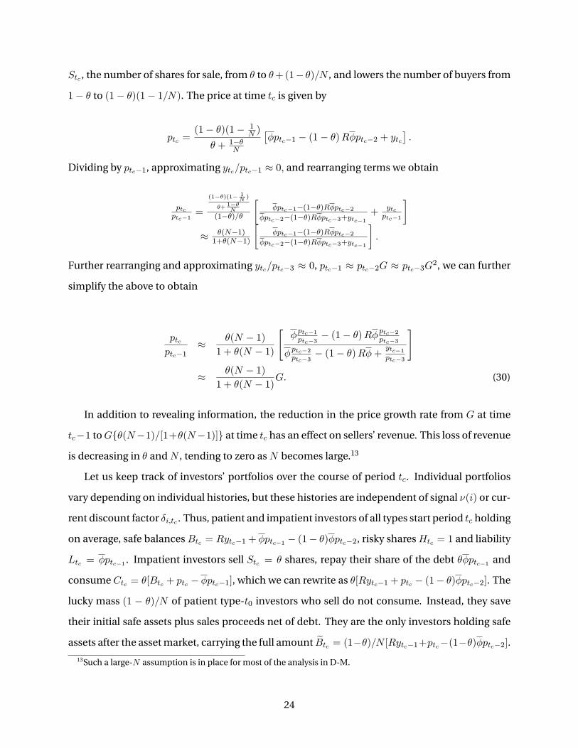
Stc , the number of shares for sale, from θ to θ+(1− θ)/N , and lowers the number of buyers from

1− θ to (1− θ)(1− 1/N). The price at time tc is given by

ptc =(1− θ)(1− 1

N )

θ + 1−θN

[φptc−1 − (1− θ)Rφptc−2 + ytc

].

Dividing by ptc−1, approximating ytc/ptc−1 ≈ 0, and rearranging terms we obtain

ptcptc−1

=

(1−θ)(1− 1N)

θ+1−θN

(1−θ)/θ

[φptc−1−(1−θ)Rφptc−2

φptc−2−(1−θ)Rφptc−3+ytc−1+ ytc

ptc−1

]≈ θ(N−1)

1+θ(N−1)

[φptc−1−(1−θ)Rφptc−2

φptc−2−(1−θ)Rφptc−3+ytc−1

].

Further rearranging and approximating ytc/ptc−3 ≈ 0, ptc−1 ≈ ptc−2G ≈ ptc−3G2, we can further

simplify the above to obtain

ptcptc−1

≈ θ(N − 1)1 + θ(N − 1)

[φptc−1ptc−3

− (1− θ)Rφptc−2ptc−3

φptc−2ptc−3

− (1− θ)Rφ+ ytc−1ptc−3

]

≈ θ(N − 1)1 + θ(N − 1)G. (30)

In addition to revealing information, the reduction in the price growth rate from G at time

tc−1 toG{θ(N−1)/[1+θ(N−1)]} at time tc has an effect on sellers’ revenue. This loss of revenue

is decreasing in θ and N , tending to zero as N becomes large.13

Let us keep track of investors’ portfolios over the course of period tc. Individual portfolios

vary depending on individual histories, but these histories are independent of signal ν(i) or cur-

rent discount factor δi,tc . Thus, patient and impatient investors of all types start period tc holding

on average, safe balances Btc = Rytc−1 + φptc−1 − (1− θ)φptc−2, risky shares Htc = 1 and liability

Ltc = φptc−1 . Impatient investors sell Stc = θ shares, repay their share of the debt θφptc−1 and

consume Ctc = θ[Btc + ptc − φptc−1], which we can rewrite as θ[Rytc−1 + ptc − (1− θ)φptc−2]. The

lucky mass (1 − θ)/N of patient type-t0 investors who sell do not consume. Instead, they save

their initial safe assets plus sales proceeds net of debt. They are the only investors holding safe

assets after the asset market, carrying the full amount Btc = (1−θ)/N [Rytc−1+ptc−(1−θ)φptc−2].13Such a large-N assumption is in place for most of the analysis in D-M.

24

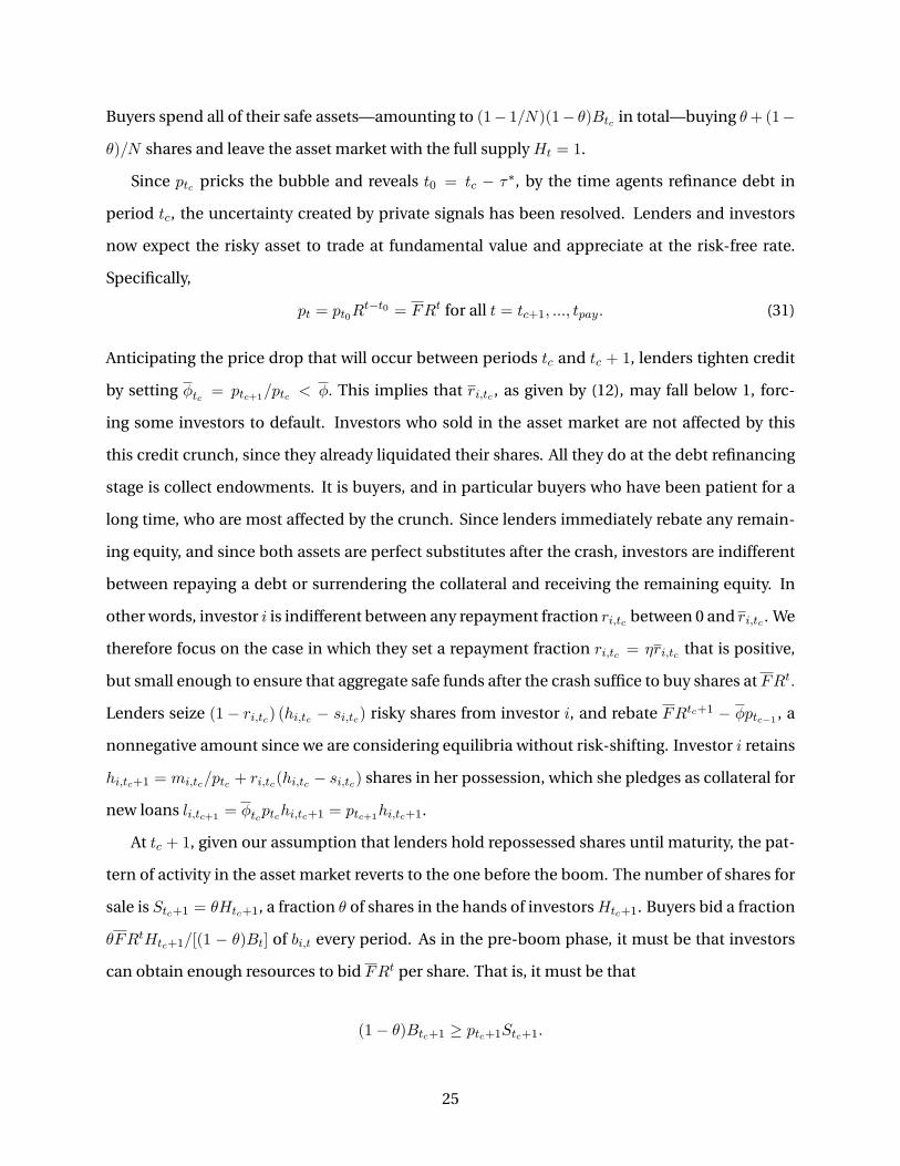
Buyers spend all of their safe assets—amounting to (1− 1/N)(1− θ)Btc in total—buying θ+(1−

θ)/N shares and leave the asset market with the full supply Ht = 1.

Since ptc pricks the bubble and reveals t0 = tc − τ∗, by the time agents refinance debt in

period tc, the uncertainty created by private signals has been resolved. Lenders and investors

now expect the risky asset to trade at fundamental value and appreciate at the risk-free rate.

Specifically,

pt = pt0Rt−t0 = FRt for all t = tc+1, ..., tpay. (31)

Anticipating the price drop that will occur between periods tc and tc + 1, lenders tighten credit

by setting φtc = ptc+1/ptc < φ. This implies that ri,tc , as given by (12), may fall below 1, forc-

ing some investors to default. Investors who sold in the asset market are not affected by this

this credit crunch, since they already liquidated their shares. All they do at the debt refinancing

stage is collect endowments. It is buyers, and in particular buyers who have been patient for a

long time, who are most affected by the crunch. Since lenders immediately rebate any remain-

ing equity, and since both assets are perfect substitutes after the crash, investors are indifferent

between repaying a debt or surrendering the collateral and receiving the remaining equity. In

other words, investor i is indifferent between any repayment fraction ri,tc between 0 and ri,tc . We

therefore focus on the case in which they set a repayment fraction ri,tc = ηri,tc that is positive,

but small enough to ensure that aggregate safe funds after the crash suffice to buy shares at FRt.

Lenders seize (1− ri,tc) (hi,tc − si,tc) risky shares from investor i, and rebate FRtc+1 − φptc−1 , a

nonnegative amount since we are considering equilibria without risk-shifting. Investor i retains

hi,tc+1 = mi,tc/ptc + ri,tc(hi,tc − si,tc) shares in her possession, which she pledges as collateral for

new loans li,tc+1 = φtcptchi,tc+1 = ptc+1hi,tc+1.

At tc + 1, given our assumption that lenders hold repossessed shares until maturity, the pat-

tern of activity in the asset market reverts to the one before the boom. The number of shares for

sale is Stc+1 = θHtc+1, a fraction θ of shares in the hands of investorsHtc+1. Buyers bid a fraction

θFRtHtc+1/[(1 − θ)Bt] of bi,t every period. As in the pre-boom phase, it must be that investors

can obtain enough resources to bid FRt per share. That is, it must be that

(1− θ)Btc+1 ≥ ptc+1Stc+1.

25

This inequality can always be guaranteed by choosing a low enough η and thus restricting the

number of shares for sale. In fact, choosing a low enough η, we can ensure that this holds for all

periods after tc until tpay.

4.3 Characterizing bubble duration

To characterize τ∗ in equilibrium, we must verify that investors are willing to play equilibrium

strategies. For expositional convenience, we focus on the case where the realization of t0 is high

enough that we can approximate pt+1 = ptG for all t ∈ {t0, ..., tc}. (Our reasoning—as we will

argue shortly—will also apply to lower realizations of t0.) Since impatient investors have zero

discount factors, it is straightforward that they are willing to sell and consume. What is not

trivial is the trade-off faced by patient investors during the boom. They must be willing to fully

invest into the risky asset, planning to leave the market at time ν(i) + τ∗, unless the bubble

bursts before. The size and duration of equilibrium bubbles depends crucially on the willingness

of patient investors to continue investing despite the crash risk. To be precise, in equilibrium

patient investors must be willing to: (i) Sell when the strategy dictates that they should sell and

(ii) Buy when the strategy dictates that they should buy. Part (i) holds for any τ∗ ≥ 1, because

an individual investor will choose to sell if she knows that other investors of her same type are

selling. That is, if investor i knows that others of her same type ν(i) are selling at t, she knows

that the price will certainly reveal the sales, and the bubble will burst in the next period.14 Part

(ii), however, is not obvious, since it is not trivial that an investor will always buy as dictated by

equilibrium strategies, especially as crash risk grows.

To understand buyers’ choices, consider a type-ν(i) investor. Her beliefs about possible val-

ues of t0 given by (22), which combines information from signal and prices. The signal ν(i)

implies that the support of t0 is the set {max{0, ν(i) − (N − 1)}, . . . , ν(i)}. The investor further

eliminates values from her support of t0 as she observes that the bubble does not burst from

period max{0, ν(i) − (N − 1)} + τ∗ onward. (If t0 had been equal to max{0, ν(i) − (N − 1)}, the

bubble would have burst at max{0, ν(i) − (N − 1)} + τ∗.) If she happens to be "first in line",

i.e., if ν(i) = t0 she unequivocally learns that t0 = ν(i) when she observes that the price at time

ν(i) − 1 + τ∗ continues to grow at the rate G. In equilibrium, she must be willing to buy until

14See D-M for a discussion of multiplicity and the role played by discrete types and noise.

26

the scheduled selling date ν(i) + τ∗, despite the fact that the probability of a crash (conditional

on the bubble not having burst yet) increases as earlier realizations of t0 are discarded. Crash

risk is highest at the start of period ν(i)− 1 + τ∗, just one period before the investor is supposed

to sell. It is at this point, with the support of t0 containing only two values {ν(i) − 1, ν(i)}, that

preemptive selling is most tempting. If investor i is willing to buy at this time, she is also willing

to buy at all earlier times.

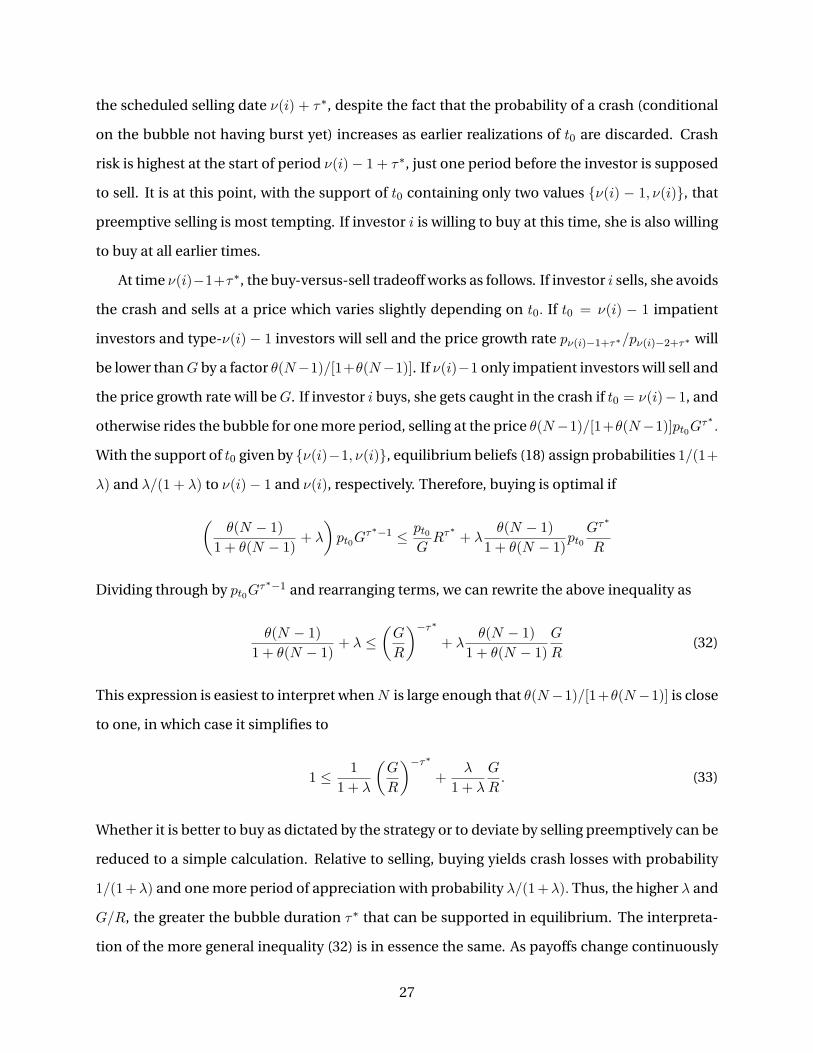
At time ν(i)−1+τ∗, the buy-versus-sell tradeoff works as follows. If investor i sells, she avoids

the crash and sells at a price which varies slightly depending on t0. If t0 = ν(i) − 1 impatient

investors and type-ν(i) − 1 investors will sell and the price growth rate pν(i)−1+τ∗/pν(i)−2+τ∗ will

be lower thanG by a factor θ(N−1)/[1+θ(N−1)]. If ν(i)−1 only impatient investors will sell and

the price growth rate will beG. If investor i buys, she gets caught in the crash if t0 = ν(i)− 1, and

otherwise rides the bubble for one more period, selling at the price θ(N−1)/[1+θ(N−1)]pt0Gτ∗.

With the support of t0 given by {ν(i)−1, ν(i)}, equilibrium beliefs (18) assign probabilities 1/(1+

λ) and λ/(1 + λ) to ν(i)− 1 and ν(i), respectively. Therefore, buying is optimal if

(θ(N − 1)

1 + θ(N − 1) + λ)pt0G

τ∗−1 ≤ pt0GRτ∗+ λ

θ(N − 1)1 + θ(N − 1)pt0

Gτ∗

R

Dividing through by pt0Gτ∗−1 and rearranging terms, we can rewrite the above inequality as

θ(N − 1)1 + θ(N − 1) + λ ≤

(G

R

)−τ∗+ λ

θ(N − 1)1 + θ(N − 1)

G

R(32)

This expression is easiest to interpret whenN is large enough that θ(N−1)/[1+θ(N−1)] is close

to one, in which case it simplifies to

1 ≤ 1

1 + λ

(G

R

)−τ∗+

λ

1 + λ

G

R. (33)

Whether it is better to buy as dictated by the strategy or to deviate by selling preemptively can be

reduced to a simple calculation. Relative to selling, buying yields crash losses with probability

1/(1+λ) and one more period of appreciation with probability λ/(1+λ). Thus, the higher λ and

G/R, the greater the bubble duration τ∗ that can be supported in equilibrium. The interpreta-

tion of the more general inequality (32) is in essence the same. As payoffs change continuously

27

as functions of θ(N − 1)/[1+ θ(N − 1)], the inequality changes quantitatively, but the qualitative

interpretation remains the same. In fact, we use (32) to characterize the set of values of τ∗ that

can be supported in equilibrium and summarize our findings in Proposition 2.

Proposition 2 Suppose that G = φ (1− θ)[1 +

√1− 4θR/φ

]/(2θ), φ ≥ 4θR, and 2B0 > φ(1 +√

1− 4θR/φ). Moreover assume that there is no risk-shifting in equilibrium. Then: (a) If G/R <

[1+θ(N−1)]/[θ(N−1)]+1/λ, equilibrium can be supported for any τ∗ between 0 and− ln({θ(N−

1)/[1 + θ(N − 1)]} + (1 − λ{θ(N − 1)/[1 + θ(N − 1)]}G/R))/ ln(G/R).(b) If G/R ≥ [1 + θ(N −

1)]/[θ(N − 1)] + 1/λ, any integer τ∗ ≥ 0, can be supported in equilibrium.

Proof. To verify that type-ν(i) investors are willing to sell at ν(i)+ τ∗, note that for any posi-

tive τ∗, if other investors of type ν(i) are selling at ν(i)+ τ∗, the price will reveal the sale and

precipitate a crash. Any investor of type ν(i) will therefore be willing to sell. To verify that type-

ν(i) investors are willing to buy as long as the boom continues and t < ν(i)+ τ∗, we first con-

sider the case in which t0 + τ∗ is large. By Lemma 1, the price growth rate pt+1/pt converges to

G = φ (1− θ)[1 +

√1− 4θR/φ

]/(2θ) as t grows, and therefore, for all types ν(i) > 0, willingness

to buy is governed by (32). Therefore, the upper bound on τ∗ given by− ln({θ(N − 1)/[1+ θ(N −

1)]}+(1−λ{θ(N − 1)/[1+ θ(N − 1)]}G/R))/ ln(G/R) is derived directly by solving (32) for τ∗. In

the event that t0 = 0, agents of type ν(i) = 0 are always willing to buy while t < t0+ τ∗ since they

know the value of t0 as soon as they observe signals. Finally, although (32) is derived for the case

where t0 + τ∗ is large, willingness to buy is even stronger if t0+ τ∗ is not large. By Lemma 1, if

2B0 > φ(1+√1− 4θR/φ), price growth rates during the boom start out higher thanG , gradually

falling towards this constant over time. Q.E.D.

In equilibria with τ∗ > N , the model generates strong bubbles in the sense of Allen et al.

(1993), where—for all t > t0 +N , all investors know with certainty that the risky asset is overval-

ued, and nevertheless continue to buy it (unless they become impatient). Up to period t0 + N ,

bubbles are weaker in the sense that some agents still believe that the boom may be fundamen-

tal.

A straightforward but important implication of Proposition 1 is the positive link between the

maximum possible bubble duration τ∗ and the LTV cap φ and the negative link between τ∗ and

the interest rateR. These results, which are in line with macroprudential wisdom, follow directly

28

from the fact that G is increasing in φ and decreasing in R, while τ∗ is increasing in G/R.

4.4 Loan-to-value limits and risk-shifting

The equilibrium analysis thus far takes absence of risk shifting as a given. We have maintained

the assumption that, either through repayment or through collateral repossession in default,

lenders fully recover principal and interest on all of their loans. In such an environment, the

competitive lending rate is equal to the risk-free rate R and investors bear the full risk of their

speculative activity.

In this Section, we show that, as long as θ and φ are not too large, bubbly equilibria with-

out risk shifting exist. While the derivation of the precise parameter thresholds is somewhat

involved, the idea behind it is quite simple. At tc − 1, lenders lend φptc−1 per unit of collateral,

but this collateral is only worth FRtc by next period’s refinancing stage. Risk shifting is avoided

if (and only if) FRtc suffices to repay φptc−1. Equilibria without risk shifting exist if this restric-

tion is compatible with condition (33) which determines bubble duration, and with the rela-

tionship between G and φ arising from the interaction between price and debt in the boom. For

tractability, we focus on the large-N case. The specific parameter restrictions and the derivation

are provided in Proposition 2 and its proof.

Absence of credit losses thus requires that is thus necessary to verify that the defaults hap-

pening at time tc do not generate credit losses. There may also be defaults at time tc + 1, given

that φptc+1 is less than φtcptc = ptc+1. However, since future collateral values are known with

certainty when loans are made at time tc, lenders perfectly foresee future prices and—although

ptc allows them to make bigger loans—adjust φtc accordingly to avoid credit losses. In sum, to

verify that condition (16) holds, we need to verify that

φptc−1 ≤ pt0Rτ∗, (34)

which, approximating ptc−1 = pt0Gtc−1, reduces to

φ

G≤(G

R

)−τ∗, (35)

29

which related the lending limit φ to the percentage price fall in the crash. If (35) holds with

equality, φ is as high as possible while still ruling out credit losses. In turn, the size of the price

drop in the crash is a crucial input to the sell-verus-wait condition that limits how large τ∗ can

be. Combining (35) with the large-N version of the sell-or-wait condition (33) and rearranging

terms yields

G

[1− λ

(G

R− 1)]≤ φ. (36)

If the conjectured strategies, lending policies and prices do indeed constitute an equilibrium,

this no-risk-shifting condition relating G and φ must hold. Moreover, as seen above, G must be

derived from φ, θ, and R according to expression (28), which we can solve for φ and rewrite as

θ

1− θG2

G− (1− θ)R = φ (37)

In Figure 6, we plot both (36) and (37) jointly in a (G,φ) diagram. For small enough values of

θ, there are two points of intersection, but only the point with the higher value ofG corresponds

to the stable root G = φ (1− θ) /(2θ)[1 +

√1− 4θR/φ

]. If θ surpasses a certain threshold, there

are no points of intersection. In that case, equilibria without risk-shifting do not exist. To solve

for said points of intersection, we equate the left-hand side of (36) to that of (37), and—after

some tedious but straightforward algebra—find that the two curves intersect at

G = R

[1− θ

2+1− 2θ ±

√[1− λθ(1− θ)]2 − 4θ(1− θ)2λ(1− θ)

](38)

Substituting G into (36) or (37) we find the corresponding level of φ.

These results are summarized in Proposition 2.

Proposition 3 Suppose thatN is large, pt+1/pt is close toG for all t ≥ t0, and that [1−λθ(1−θ)]2 ≥

4θ(1 − θ). Then, there is a nonempty region of the parameter space in which bubbly equilibria

without risk-shifting exist. Moreover, bubbles in this region can become arbitrarily large.

Proof. Of all loans made by lenders, those made at time tc−1 are most likely to become ’underwa-

ter’ loans and generate credit losses. At tc − 1, lenders extend loans amounting to φptc−1 per unit

of collateral. Loans collateralized by units that are sold at tc are easily repaid, since ptc is higher

than ptc−1 . However, the lower growth rate of the price reveals that the bubble has burst, lowering

30

the value of the bubble to FRtc . This value is the same, regardless of whether lenders sell the seized

shares or hold them to collect the dividend. It is thus necessary to verify that the defaults hap-

pening at time tc do not generate credit losses. There may not be credit losses for loans made after

the crash, since future collateral values are known with certainty when loans are made and thus

lenders adjust loan sizes. Specifically, at time tc, although ptc allows them to make bigger loans,

lenders adjust φtc accordingly to avoid credit losses. In sum, to verify that condition (16) holds, we

need to verify that

φptc−1 ≤ pt0Rτ∗, (39)

which, approximating ptc−1 = pt0Gtc−1, reduces to

φ

G≤(G

R

)−τ∗, (40)

which related the lending limit φ to the percentage price fall in the crash. If (35) holds with equal-

ity, φ is as high as possible while still ruling out credit losses. In turn, the size of the price drop

in the crash is a crucial input to the sell-versus-wait condition that limits how large τ∗ can be.

Combining (35) with the large-N version of the sell-or-wait condition (33) and rearranging terms

yields

G

[1− λ

(G

R− 1)]≤ φ. (41)

If the conjectured strategies, lending policies and prices do indeed constitute an equilibrium, this

no-risk-shifting condition relatingG and φmust hold. Moreover, as seen above,Gmust be derived

from φ, θ, and R according to expression (28), which we can solve for φ and rewrite as

θ

1− θG2

G− (1− θ)R = φ (42)

In Figure 6, we plot both (36) and (37) jointly in a (G,φ) diagram. For small enough values of θ—

specifically if [1− λθ(1− θ)]2 − 4θ(1− θ)—there are two points of intersection, but only the point

with the higher value ofG corresponds to the stable rootG = φ (1− θ) /(2θ)[1 +

√1− 4θR/φ

]. If

θ surpasses a certain threshold, there are no points of intersection. In that case, equilibria without

risk-shifting do not exist. To solve for said points of intersection, we equate the left-hand side of

31

(36) to that of (37), and—after some tedious but straightforward algebra—find that the two curves

intersect at

G = R

[1− θ

2+1− 2θ ±

√[1− λθ(1− θ)]2 − 4θ(1− θ)2λ(1− θ)

](43)

Substituting this expression for G into (36) or (37) we find the corresponding level of φ. Finally, it

follows from (43) and (36), that by lowering θ—and φ falling in order to ensure risk-shifting—one

can always raise G and τ∗. Q.E.D.

4.5 Discussion and Extensions

Binding borrowing constraints are essential because they allow us to circumvent the impossibil-

ity results by Tirole (1982). As in DM, there are two reasons for this. First, investors know that if

the bubble does not burst, it will grow fuelled by more funds. The prospect of continued growth

provides an incentive to ride the bubble that is absent if all the funds that are expected to ar-

rive are already there, in which case trading overvalued assets is a zero-sum game. The second

reason why borrowing constraints are essential is informational. Since investors bid as much

as they can borrow, their private estimate of the worth of the risky asset is not revealed. In the

absence of borrowing constraints, uncertainty about t0 would be revealed as soon as the boom

began.15

In the interest of tractability and parsimony, we have sought to make this credit-based exten-

sion while staying as close as possible to DM. In particular, the key investor trade-offs that limit

bubble duration unchanged are not affected by risk-shifting or other new considerations arising

from the credit market. Nevertheless, and although we believe that it is clearest to introduce

changes one at a time, it is interesting to discuss how alternative assumptions would influence

results. In particular, we discuss liquidation of repossessed assets, loan-to-income requirements

and endogenous timing of refinancing.

15Another assumption with key informational implications is the trading protocol under which that agents makebuy/sell decisions in a first stage and observe prices in a second stage. This allows type-t0 agents to sell at tc, sinceother agents commit to buying in the first stage of the period and cannot withdraw their bids after observing the price.This protocol resembles an exchange with market orders, which are always filled with certainty, but without a priceguarantee. Under Walrasian timing—or in a market with limit orders—our results would not obtain, since buyers attc would be able to condition their purchase on the price. Only if there was enough noise in the price process, thisassumption could be relaxed, since buyers would not be able to distinguish the beginning of the crash from randomday-to-day fluctuations. D-M incorporates some of these ideas, although he does not allow enough noise to allow forWalrasian timing.

32

Our assumption that lenders hold repossessed shares until maturity is analytically conve-

nient, and weakly optimal for lenders. However, the scenario in which lenders liquidate repos-

sessed assets appears to be more realistic. If lenders liquidates collateral, they would only be

concerned with the liquidation price to the extent that it allowed them to recover their debt.

Thus, in equilibria in which there was positive equity after the crash, a glut of liquidations could

depress prices below fundamental value. As long as price remained above the remaining debt,

lenders would not be affected by the decrease in price.16 This ’undershooting’ pattern where

prices may recover after a period of defaults and liquidations may be reminiscent of recent

events in US housing and equity markets. Unfortunately, incorporating this in our model would

greatly complicate the notation, exposition and analysis. Characterizing maximum bubble du-

ration τ∗ would no longer be analytically feasible, since inequality (32) would have to be mod-

ified to account for the greater crash losses, as well as the opportunity of early sellers to profit

twice by reentering the market at below-fundamental prices.

The model could also be extended to accommodate risk-shifting. In that case, borrowers

in default would be ’under water’ and thus the issue of undershooting would not arise, since

lenders would be motivated to maximize the sales price. The beliefs of lenders, which do not

play a role in our model, would become crucial in the risk-shifting case. They would determine

interest rates, credit limits, and thus the growth rate of the bubble and its maximum duration.

Our conjecture is that risk-shifting would be conducive to bubbles, since investors would be able

to pass losses to lenders, although this effect would be attenuated by higher interest rates.

Another common factor affecting lending standards in practice is the loan-to-income ra-

tio. A cross-country study by Lim, et al. (2011) provides empirical support for this idea. The

authors compare the use and performance of loan-to-value constraints versus debt-to-income

constraints together with other macroprudential policy tools. Their regression results (p. 53)

show that the implementation of a debt-to-income cap is more effective than a loan-to-value

cap in reducing the growth rates of real estate prices and credit. In fact, in our model, loan-to-

endowment or loan-to-dividend caps would not give rise to booming dynamics, and thus would

preclude bubbles. That said, this requirement could also prevent prices from reaching fudamen-

16In fact, this is a commonly used argument to explain why foreclosures are sold at discounted prices. If it is costlyfor lenders to hold a property that is ’above water’, they have a strong incentive to lower the price in order to sellquickly.

33

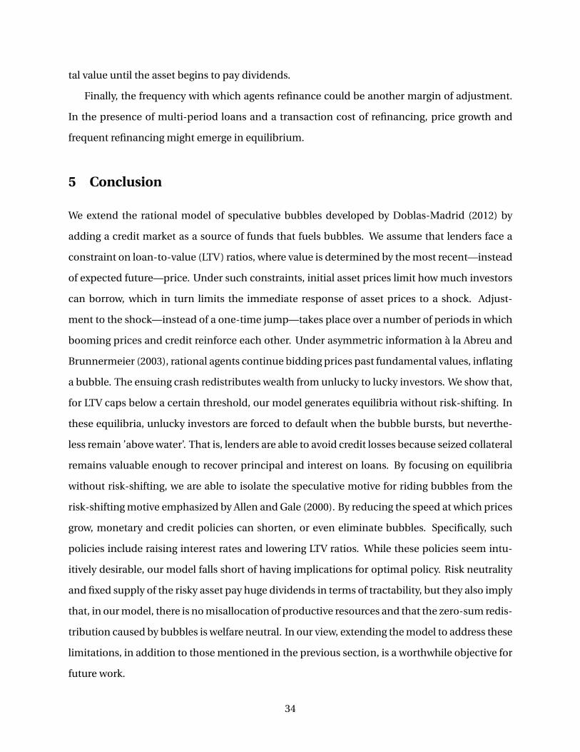
tal value until the asset begins to pay dividends.

Finally, the frequency with which agents refinance could be another margin of adjustment.

In the presence of multi-period loans and a transaction cost of refinancing, price growth and

frequent refinancing might emerge in equilibrium.

5 Conclusion

We extend the rational model of speculative bubbles developed by Doblas-Madrid (2012) by

adding a credit market as a source of funds that fuels bubbles. We assume that lenders face a

constraint on loan-to-value (LTV) ratios, where value is determined by the most recent—instead

of expected future—price. Under such constraints, initial asset prices limit how much investors

can borrow, which in turn limits the immediate response of asset prices to a shock. Adjust-

ment to the shock—instead of a one-time jump—takes place over a number of periods in which

booming prices and credit reinforce each other. Under asymmetric information à la Abreu and

Brunnermeier (2003), rational agents continue bidding prices past fundamental values, inflating

a bubble. The ensuing crash redistributes wealth from unlucky to lucky investors. We show that,

for LTV caps below a certain threshold, our model generates equilibria without risk-shifting. In

these equilibria, unlucky investors are forced to default when the bubble bursts, but neverthe-

less remain ’above water’. That is, lenders are able to avoid credit losses because seized collateral

remains valuable enough to recover principal and interest on loans. By focusing on equilibria

without risk-shifting, we are able to isolate the speculative motive for riding bubbles from the

risk-shifting motive emphasized by Allen and Gale (2000). By reducing the speed at which prices

grow, monetary and credit policies can shorten, or even eliminate bubbles. Specifically, such

policies include raising interest rates and lowering LTV ratios. While these policies seem intu-

itively desirable, our model falls short of having implications for optimal policy. Risk neutrality

and fixed supply of the risky asset pay huge dividends in terms of tractability, but they also imply

that, in our model, there is no misallocation of productive resources and that the zero-sum redis-

tribution caused by bubbles is welfare neutral. In our view, extending the model to address these

limitations, in addition to those mentioned in the previous section, is a worthwhile objective for

future work.

34

References

[1] Abreu D. and M. Brunnermeier, 2003 Bubbles and crashes, Econometrica 71, 173-204.

[2] Allen F., S. Morris and A. Postlewaite 1993 Finite bubbles with short sales constraints and

asymmetric information, Journal of Economic Theory 61, 209-229.

[3] Allen, F. and D. Gale 2000 Bubbles and crises, Economic Journal 110, 236-255.

[4] Barlevy, G. 2014 A leverage-based model of speculative bubbles, Journal of Economic The-

ory 153, 459–505.

[5] Barlevy, G. 2015 Bubbles and fools, Federal Reserve Bank of Chicago, Economic Perspec-

tives 2Q, 54-76.

[6] Barlevy, G. and J.D.M. Fisher 2010, Mortgage choices and housing speculation, Federal Re-

serve Bank of Chicago, Working Paper 2010-12

[7] Borio, C. and P. Lowe 2002 Asset prices, financial and monetary stability: Exploring the

nexus, Bank for International Settlements Working Paper 114.

[8] Berkovec, J., Y. Chang, and D.A. McManus 2012 Alternative lending channels and the crisis

in U.S. housing markets, Real Estate Economics 40, Special Issue No. 1, S8-S31.

[9] Conlon, J., 2004 Simple finite horizon bubbles robust to higher order knowledge, Econo-

metrica 72, 927-936.

[10] Conlon, J., 2015 Should central banks burst bubbles? Some microeconomic issues, Eco-

nomic Journal 125, 141-161.

[11] Doblas-Madrid, A. 2012 A robust model of bubbles with multidimensional uncertainty,

Econometrica, 80, 1245-93.

[12] Dell’Ariccia, G,. D. Igan, and L. Laeven 2012 Credit booms and lending standards: Evidence

from the subprime mortgage market, Journal of Money Credit and Banking 44, 367-384.

[13] Galí, J. 2014. Monetary policy and rational asset price bubbles, American Economic Review,

104, 721-52.

35

[14] Glick, R. and K.J. Lansing 2010 Global household leverage, house prices and consumption,

Federal Reserve Bank of San Francisco Economic Letter 2010-01 (January 11).

[15] Goetzmann, W.N., L. Peng and J. Yen 2012 The subprime crisis and house price apprecia-

tion, Journal of Real Estate Finance and Economics 44, 36-56.

[16] International Monetary Fund 2012 Dealing with household debt, Chapter 3 of World Eco-

nomic Outlook (WEO), Growth Resuming, Dangers Remain (April).

[17] Jordà, O., M. Schularick, and A.M. Taylor 2016 Leveraged bubbles, Journal of Monetary Eco-

nomics, forthcoming.

[18] Kindleberger, C.P and R. Aliber 2005 Manias, panics, and crashes: A history of financial

crises, 5th edition. Palgrave Macmillan.

[19] Kiyotaki, N, and J. Moore 1997 Credit Cycles, Journal of Political Economy 105, 211-248.

[20] Lim, C., F. Columba, A. Costa, P. Kongsamut, A. Otani, M. Saiyid, T. Wezel, and X. Wu 2011

Macroprudential Policy: What Instruments and How to Use Them? IMF Working Paper

11/238.

[21] Martin, A. and J. Ventura 2012 Economic growth with bubbles, American Economic Review

102, 3033-3058.

[22] Mian, A. and A. Sufi 2009 The consequences of mortgage credit expansion: Evidence from

the U.S. mortgage default crisis, Quarterly Journal of Economics 124, 1449-1496.

[23] Minsky, H.P. 1986 Stabilizing an Unstable Economy, Yale University Press.

[24] Pavlov, A. and S.Wachter 2011 Subprime lending and real estate prices, Real Estate Eco-

nomics 39, 1-17.

[25] U.S. Financial Crisis Inquiry Commission 2011 Final Report on the Causes of the Financial

and Economic Crisis in the United States, Pursuant to Public Law 111-2 (January).

36

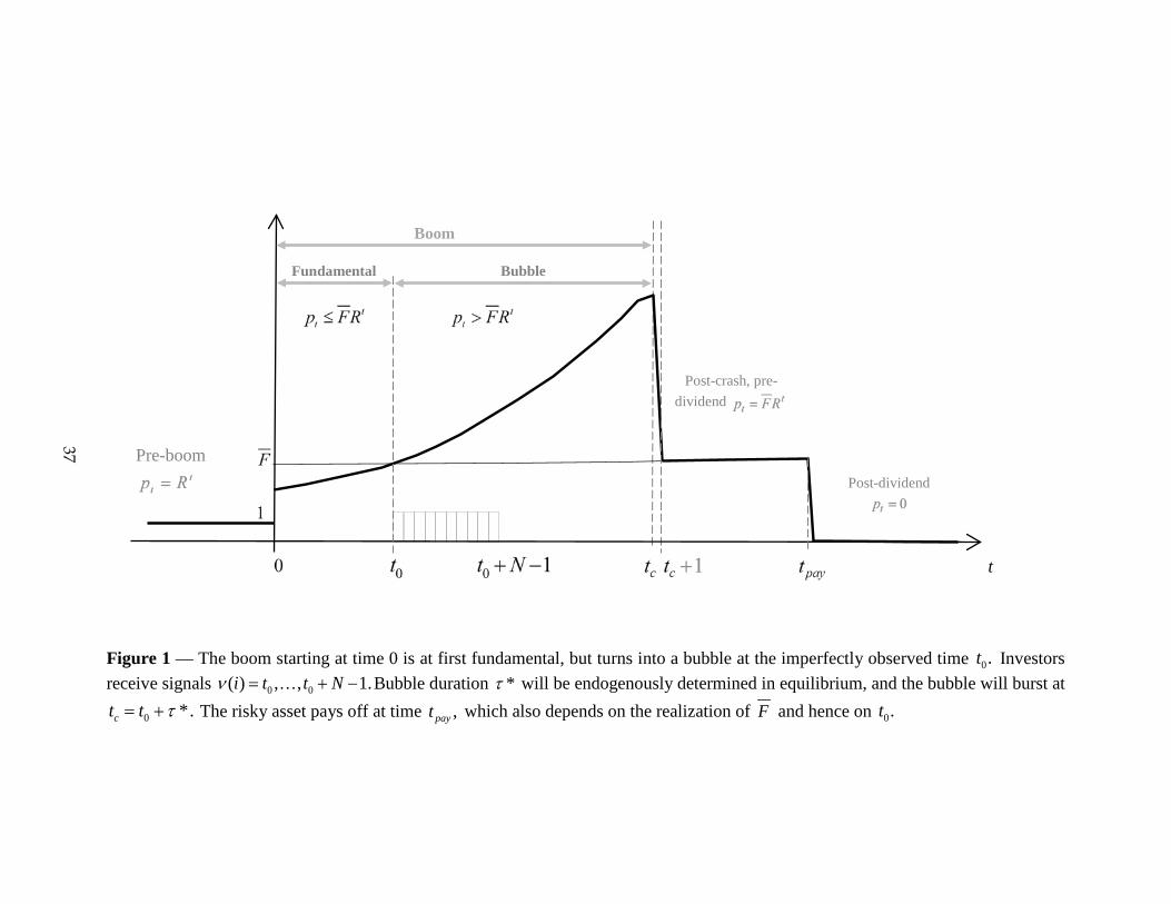
37

Figure 1 — The boom starting at time 0 is at first fundamental, but turns into a bubble at the imperfectly observed time 0.t Investors receive signals 0 0( ) , , 1.i t t Nν = + − Bubble duration *τ will be endogenously determined in equilibrium, and the bubble will burst at

0 *.ct t τ= + The risky asset pays off at time ,payt which also depends on the realization of F and hence on 0.t

Boom

Fundamental Bubble

Post-crash, pre-dividend

t

Pre-boom Post-dividend

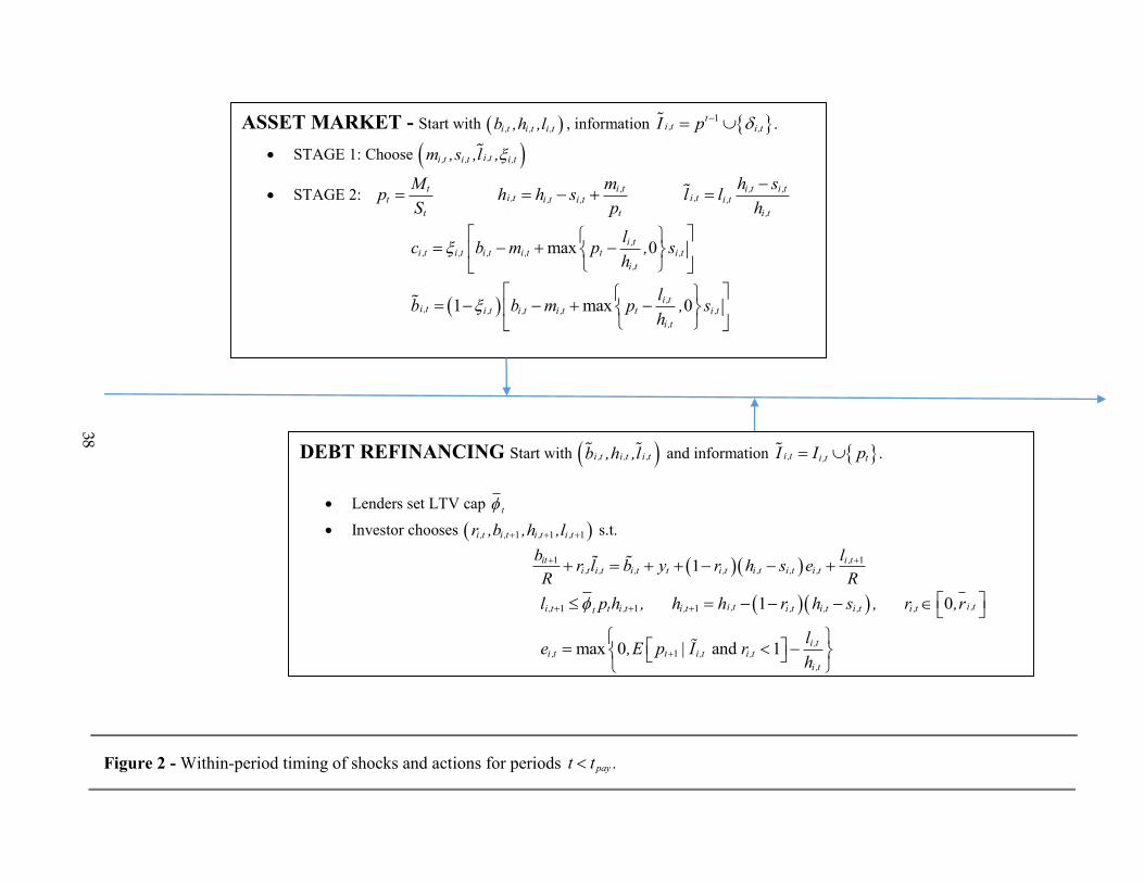
ASSET MARKET - Start with ( )i ,t i ,t i ,tb ,h ,l , information { }1ti ,t i ,tI p .δ−= ∪

• STAGE 1: Choose ( )i ,ti ,t i ,t i ,tm ,s ,l ,ξ

• STAGE 2: t i ,t i ,t i ,ti ,t i ,tt i ,t i ,t i ,t

t t i ,t

M m h sp h h s l lS p h

−= = − + =

( )

max 0

1 max 0

i ,ti ,t i ,t i ,t i ,t t i ,t

i ,t

i ,ti ,t i ,t i ,t i ,t t i ,t

i ,t

lc b m p , sh

lb b m p , sh

ξ

ξ

= − + −

= − − + −

DEBT REFINANCING Start with ( )i ,t i ,t i ,tb ,h ,l and information { }i ,t i ,t tI I p .= ∪

• Lenders set LTV cap tφ

• Investor chooses ( )1 1 1i ,t i ,t i ,t i ,tr ,b ,h ,l+ + + s.t.

( )( )1 11it i ,ti ,t i ,t i ,t t i ,t i ,t i ,t i ,t

b lr l b y r h s eR R+ ++ = + + − − +

( )( )1 1 1

1

1 0

max 0 and 1

i ,ti ,ti ,t t i ,t i ,t i ,t i ,t i ,t i ,tt

i ,ti ,t t i ,t i ,t

i ,t

l p h , h h r h s , r ,r

le ,E p | I rh

φ+ + +

+

≤ = − − − ∈ = < −

Figure 2 - Within-period timing of shocks and actions for periods payt t .<

38

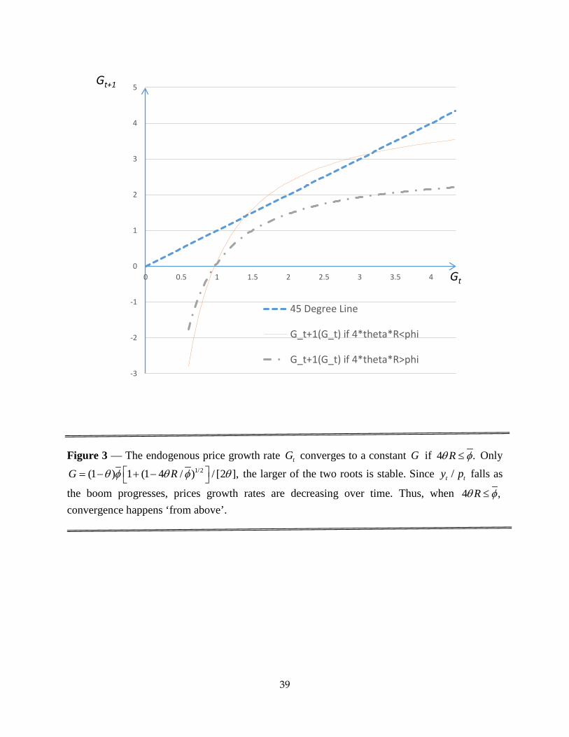
Figure 3 — The endogenous price growth rate tG converges to a constant G if 4 .Rθ φ≤ Only

1/2(1 ) 1 (1 4 / ) / [2 ],G Rθ φ θ φ θ = − + − the larger of the two roots is stable. Since /t ty p falls as

the boom progresses, prices growth rates are decreasing over time. Thus, when 4 ,Rθ φ≤convergence happens ‘from above’.

-3

-2

-1

0

1

2

3

4

5

0 0.5 1 1.5 2 2.5 3 3.5 4

45 Degree Line

G_t+1(G_t) if 4*theta*R<phi

G_t+1(G_t) if 4*theta*R>phi

Gt+1

Gt

39

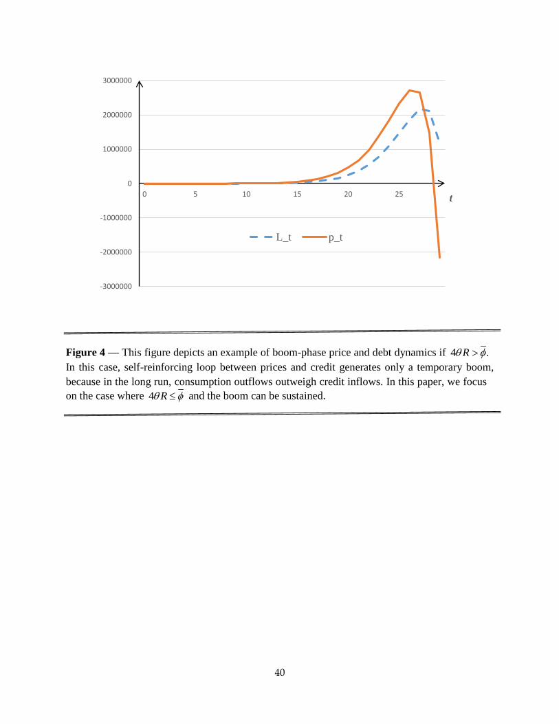
Figure 4 — This figure depicts an example of boom-phase price and debt dynamics if 4 .Rθ φ>

In this case, self-reinforcing loop between prices and credit generates only a temporary boom, because in the long run, consumption outflows outweigh credit inflows. In this paper, we focuson the case where 4 Rθ φ≤ and the boom can be sustained.

-3000000

-2000000

-1000000

0

1000000

2000000

3000000

0 5 10 15 20 25 t

L_t p_t

40

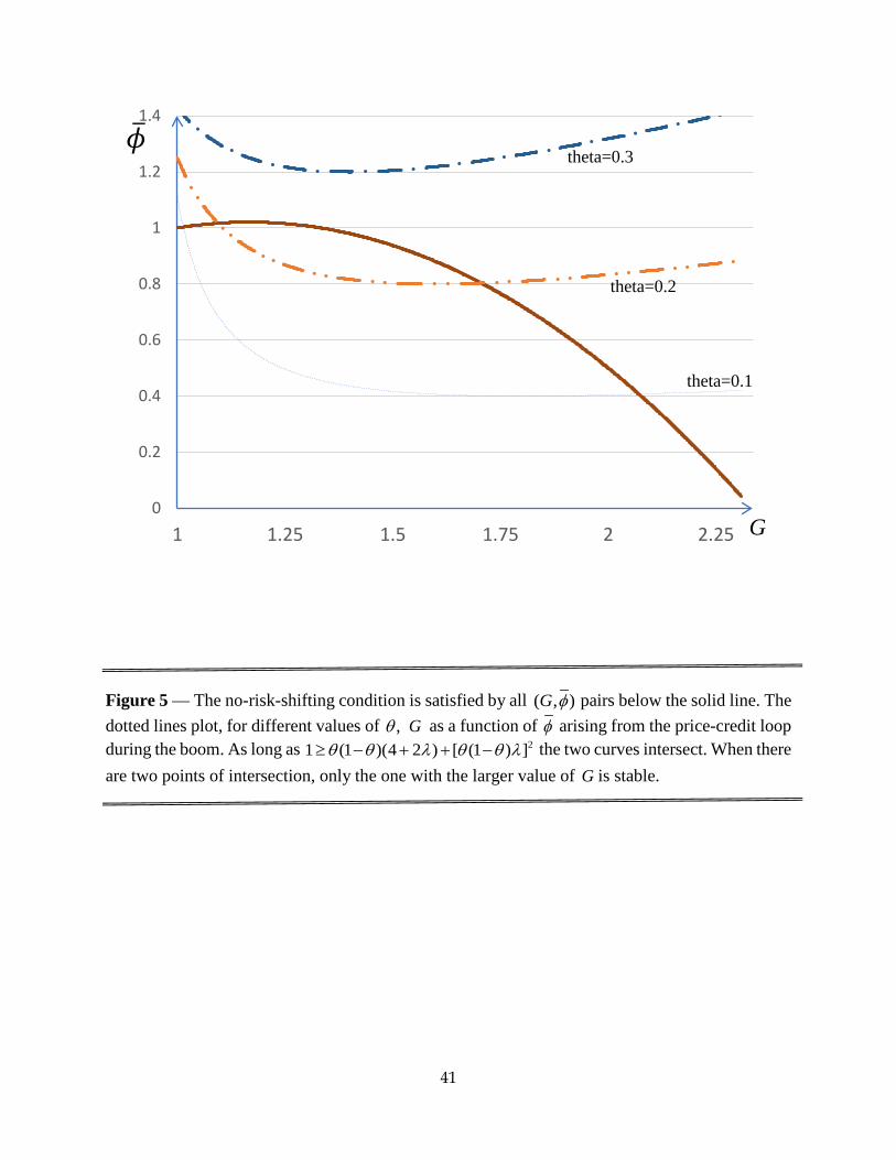
Figure 5 — The no-risk-shifting condition is satisfied by all ( , )G φ pairs below the solid line. The dotted lines plot, for different values of ,θ G as a function of φ arising from the price-credit loop during the boom. As long as 21 (1 )(4 2 ) [ (1 ) ]θ θ λ θ θ λ≥ − + + − the two curves intersect. When there are two points of intersection, only the one with the larger value of G is stable.

0

0.2

0.4

0.6

0.8

1

1.2

1.4

1 1.25 1.5 1.75 2 2.25

�𝜙𝜙

G

theta=0.3

theta=0.1

theta=0.2

41