Credit risk models: An analysis of default correlation

Michigan Technological University Michigan Technological University

Digital Commons @ Michigan Tech Digital Commons @ Michigan Tech

College of Business Publications College of Business

2010

Credit risk models: An analysis of default correlation Credit risk models: An analysis of default correlation

Howard Qi Michigan Technological University, [email protected]

Yan Alice Xie University of Michigan - Dearborn

Sheen Liu Washington State University - Vancouver

Follow this and additional works at: https://digitalcommons.mtu.edu/business-fp

Part of the Business Commons, and the Finance Commons

Recommended Citation Recommended Citation Qi, H., Xie, Y. A., & Liu, S. (2010). Credit risk models: An analysis of default correlation. The International Journal of Business and Finance Research, 4(1), 37-49. Retrieved from: https://digitalcommons.mtu.edu/business-fp/13

Follow this and additional works at: https://digitalcommons.mtu.edu/business-fp

Part of the Business Commons, and the Finance Commons

http://www.mtu.edu/

http://www.mtu.edu/

https://digitalcommons.mtu.edu/

https://digitalcommons.mtu.edu/business-fp

https://digitalcommons.mtu.edu/business

https://digitalcommons.mtu.edu/business-fp?utm_source=digitalcommons.mtu.edu%2Fbusiness-fp%2F13&utm_medium=PDF&utm_campaign=PDFCoverPages

http://network.bepress.com/hgg/discipline/622?utm_source=digitalcommons.mtu.edu%2Fbusiness-fp%2F13&utm_medium=PDF&utm_campaign=PDFCoverPages


https://digitalcommons.mtu.edu/business-fp?utm_source=digitalcommons.mtu.edu%2Fbusiness-fp%2F13&utm_medium=PDF&utm_campaign=PDFCoverPages



The International Journal of Business and Finance Research ♦ Volume 4 ♦ Number 1 ♦ 2010

CREDIT RISK MODELS: AN ANALYSIS OF DEFAULT CORRELATION

Howard Qi, Michigan Tech University Yan Alice Xie, University of Michigan – Dearborn

Sheen Liu, Washington State University – Vancouver

ABSTRACT This paper examines one of the major problems in credit risk models widely used in the financial industry to forecast future defaults and bankruptcies. We find that even after proper calibration, a representative credit risk model can severely underestimate default correlation. We further find that a likely reason for the underestimation of default correlation is the problematic common practice in the financial industry of using observable equity correlation as a proxy for unobservable asset correlation when the model is applied to predict default correlation. However, our results show that this proxy in common practice is not valid. JEL: G01; G21; G31 KEYWORDS: Credit risk model, default correlation, model risk, financial crisis INTRODUCTION

he current financial crisis has shaken the whole financial market and profoundly affected the global economy. Numerous innovative financial instruments have been blamed for causing the crisis, such as Collateralized Debt Obligations (CDOs), Mortgage Backed Securities (MBS), and

Credit Default Swaps (CDS), although these instruments were originally devised to manage credit risk and implement risk-sharing efficiently, thereby improving the stability of the financial markets. In contrast, these innovative financial instruments fail to attain their original goals. One of the major reasons is the incorrect pricing of credit risk in these financial instruments. For example, the credit risk models used by American International Group (AIG), which wrote billions of CDS to provide insurance for mortgages, grossly underestimate the credit risk of insured mortgages. When unexpected multiple defaults on mortgages happen simultaneously, as they did in the recent financial crisis, the CDS claims AIG owed significantly exceeded the premiums the company received from CDS. Subsequently, AIG became nearly insolvent and the US Government had to bail it out. Similarly, the credit risk models used by rating agencies such as Fitch, Moody’s, and Standard and Poor’s, all failed to predict the default rates of subprime mortgages and greatly overrated subprime mortgage-backed securities. The modeling error led to write-downs of more than $500 billion subprime-related securities by financial firms around the world. The above evidence shows that the use of flawed credit risk models has brought significantly unfavorable outcome to financial firms. In modern financial markets, financial firms rely heavily on models for pricing financial instruments or managing risks. In particular, in the past decade, the success of quantitative financial modeling has made the decision-making process in financial firms more reliant on (sophisticated) quantitative models. Financial researchers and practitioners developed the increasing belief that risk was under control to the extent that many, for example, de Chassart and Firer (2004), believed that it was not as difficult as once thought to forecast and outperform the volatile market. However, past success by no means guarantees future success. A number of studies on the current financial crisis have addressed the problems with credit risk models the financial industry uses. For

T

37

H. Qi et al The International Journal of Business and Finance Research ♦ Vol. 4 ♦ No. 1 ♦ 2010

example, Chancellor (2007) and Jameson (2008) argue that some false assumptions make risk models dysfunctional. Buchanan (2008) claims the existing credit risk models tend to underestimate the probability of sudden large events. Lohr (2008) and Mollenkamp et al. (2008) believe that human factors cause the risk models to be incorrectly applied. However, one of the critical problems in credit risk models, which is the inability of the models to accurately predict default correlation, has not been widely noted in studies on the current financial crisis. If a credit risk model cannot estimate default correlation accurately, the estimated joint default rates of the securities are problematic. For example, one of the reasons behind the fallout of AIG is that its credit risk model underestimated the correlation between defaults on insured mortgages, thereby greatly underpredicting the joint default rates of the mortgages. Consequently, AIG suffered record losses from selling CDS. In this study, we revisit a representative default correlation model, Zhou’s credit risk model (2001), to examine the ability of the model to predict default correlations between bonds of different ratings. Zhou’s model is built on a first-time-passage structural framework that specifies default as an event that occurs when the firm’s asset value falls below the default boundary for the first time. Default correlation is generated by the correlation between two firms’ underlying assets. Along the same line, financial practitioners proposed other structural credit risk models, such as Moody’s KMV model, JP Morgan’s CreditMetricsTM risk model, and Fitch’s VECTOR. However, the difficulty in implementing structural credit risk models is that the value of firm assets is unobservable due to the unobservable components of firm value, i.e. tax shields and expected bankruptcy costs. To get around this difficulty, the common practice is to use observable equity correlation as a proxy for unobservable asset correlation. For instance, Zhou (2001) assumed equal asset and equity correlations, and picked a constant equity correlation (i.e., 0.4) for all bond ratings. To utilize the KMV model, the CreditMetricsTM model, and Fitch’s VECTOR model, financial practitioners commonly pick an asset correlation or set the asset correlation equal to equity correlation. For example, Fitch Ratings point out that the direct measurement of asset correlation between firms is impossible given that historical firm value time series are generally not available; consequently, Fitch uses equity correlation to approximate asset correlation when implementing its VECTOR model (see Global Rating Criteria for Collateralized Debt Obligations, 2003, Fitch Ratings). This practice has three major flaws. First, equity correlation and asset correlation can differ substantially. In particular, as financial leverage increases, equity deviates more from asset and the difference between equity correlation and asset correlation widens. Second, equity correlation is likely to vary, rather than remain constant, for different ratings. Third, it is inappropriate to use an ad hoc number (e.g., 0.4) for equity (or asset) correlation. While the ad hoc number may make the model fit historical default correlations well, it cannot provide useful information on ex post predictions of default correlation. Our analysis shows that Zhou’s structural credit risk model significantly underestimates default correlation between differently rated bonds. Our results suggest that while structural credit risk models can adequately predict default rates of a single risky bond, they fail to predict joint default rates if multiple defaults happen simultaneously. A major reason is the improper common practice that approximates asset correlation with equity correlation when financial practitioners use the model to predict default correlation. The remainder of the paper is organized as follows: Section 2 briefly reviews the relevant literature. Section 3 explains the relation between default correlation and estimation of joint default rates. Section 4 describes the data and Zhou’s structural credit risk model (2001). Section 5 provides analysis and discussions of estimation results, and Section 6 concludes the paper.

38


LITERATURE REVIEW To better understand the problems inherent in credit risk models, we briefly review the two families of credit risk models in the finance literature: reduced form models and structural models. Reduced form models treat default as a process determined by exogenous state variables. Albeit easier to implement, this type of models cannot be used to estimate default correlation based on the correlation between firm characteristics (see among others, Duffie and Singleton, 1997, 1999; Jarrow et al., 1997; Jarrow and Turnbull, 1995; Lando, 1998; Madan and Unal, 1998, 2000). Structural models, in contrast, use firm characteristics, such as financial leverage and asset return volatility, to predict default probability and default correlation between two firms. The model assumes that default is triggered when firm value falls below some threshold (default boundary). The structural model was pioneered by the seminal works of Black and Scholes (1973, B-S hereafter) and Merton (1974). Their models assume that default can only happen at debt maturity. As illustrated by recent mortgage default, this is not a realistic assumption, and this unrealistic assumption results in the underestimation of default probability. To allow for default before debt maturity, Black and Cox (1976) introduced the first-passage-time (FPT) model that specifies default as an event when the firm’s asset value crosses the default boundary for the first time. A great number of empirical works have shown that the FPT model is superior to the B-S and Merton models in predicting bond yield and credit risk of a single risky bond. At present, the FPT model is widely used to estimate credit risk in the financial industry. Based on the FPT structural framework, Zhou (2001) developed a seminal model for default correlation generated by the correlation between two firms’ underlying assets. To account for contagious credit risk effects, Giesecke (2003, 2006) derived a model by assuming correlated default boundaries in addition to correlated firm values. The idea is that default boundaries are uncertain. When one firm defaults, another firm’s default boundary is revealed. The original purpose of the model was to boost default correlation prediction. However, we note that this mechanism could also decrease default correlation prediction because if the revealed second firm’s default boundary is below what is expected, the model would generate a lower default correlation. Meanwhile, financial practitioners also proposed various credit risk models using the structural framework, including Moody’s KMV model, JP Morgan’s CreditMetricsTM risk model, and Fitch Ratings VECTOR. The basic idea in Moody’s KMV model is that a firm will default on its debt obligations if the firm value drops below its default point, which is defined as the sum of the value of short-term debt and the value of a portion of long-term debt. An important feature of the KMV model is that a single measure of default risk – distance-to-default is calculated to estimate default probability. Distance-to-default is calculated as the difference between the firm value and the default point divided by the size of one standard deviation move in the firm value (see Crosbie and Bohn, 2003). JP Morgan’s CreditMetricsTM is the first model for assessing credit risk in portfolios due to changes in debt value caused by changes in obligor credit quality. This model includes changes in value caused not only by possible default events, but also by upgrades and downgrades in credit quality. Also, this model assesses the value-at-risk (VaR), not just the expected losses and, as a result, the model enables a firm to have an integrated view of credit risk across its entire organization (see Gupton et al., 1997). Fitch’s VECTOR default model allows users to estimate the effect of rating transition. It is Fitch's core CDO modeling tool that allows users to analyze rating transition risk and spread migration in leveraged super-senior (LSS) transactions in addition to the traditional default and recovery risks normally associated with CDO transactions. LSS transaction was considered one of the most successful innovative derivative products on Wall Street in 2005. For example, in a LSS transaction with 10 times leverage, a

39


5% change in the value of the underlying super senior tranche is equivalent to a 50% change in the market value of the funded investment (see DerivativeFitch, 2004). However, a common problem in implementing structural credit risk models is that the value of firm assets is unobservable. To deal with this difficulty, the common practice is to use the observable equity correlation as a proxy for unobservable asset correlation. In the following sections, we show that this common practice is problematic. DEFAULT CORRELATION Default events are rarely independent and it is not uncommon for multiple defaults to be triggered at the same time. For example, plummeting housing prices and climbing interest rates triggered an unprecedented number of defaults on subprime mortgages across the country over the same period. Therefore, to price credit risk accurately and perform risk management effectively, we need to estimate default rates of multiple defaults (or joint default probability). In this section, we use a simple numerical example to demonstrate how default correlation affects the estimation of joint default probability. Denote the default status of two firms over a given horizon T as

( )1 if firm defaults by 0 otherwisei

i TTω

=

(1)

The joint default probability is written as [ ][ ] [ ] [ ] [ ]

1 2 1 2

1 2 1 2

( ( ) 1 an d ( ) 1) ( ) ( )

( ) ( ) ( ) ( )D

P T T E T T

E T E T Var T Var T

ω ω ω ω

ω ω ρ ω ω

= = = ⋅

= ⋅ + (2)

Because ω1(T) and ω2(T) are Bernoulli binomial random variables, we have ( ) ( ( ) 1)

( ) ( ( ) 1) 1 ( ( ) 1)

E T P Ti i

Va r T P T P Ti i i

ω ω

ω ω ω

= = = = ⋅ − =

(3)

and ρD stands for default correlation. Suppose that the default probability of the bond issued by firm A is 8%, i.e. [ ]1( ) 1 8%E Tω = = , and that of the bond issued by firm B is 5%, i.e. [ ]2 ( ) 1 5%E Tω = = . If the defaults of bond A and bond B are independent, the joint default probability ( )1 2( ( ) 1 and ( ) 1P T Tω ω= = should be equal to 8% × 5% = 0.4%. However, if the default correlation between bonds A and B is 0.4, the joint default probability is equal to

1 2( ( ) 1 and ( ) 1) 8% 5% 0.4 8%(1 8%)5%(1 5%) 2.77%P T Tω ω= = = × + − − = . The numerical example shows that if these two defaults are correlated but the correlation is ignored, the joint default probability can be underestimated by a factor of seven. In practice, the model error could create huge losses for the financial firms. In the following section, we examine the ability of the structural credit risk models to predict default correlation. Specifically, we test Zhou’s default correlation model. DATA AND METHODOLOGY To test the ability of structural credit risk models to predict default correlation, we first estimate equity correlation that is commonly used as a proxy for asset correlation, which is a key input variable in the

40


default correlation model. Next, we present our methodology by describing Zhou’s default correlation model. Data Description We use daily stock returns to estimate equity correlation for firms across different ratings during the period 1970 to 1993. The reason we chose the sample period of 1970 to 1993 is to compare the estimated default correlations by Zhou’s model (2001) with the historical default correlations reported by Lucas (1995), who only reports the historical default correlations over this sample period. We obtain daily stock returns from CRSP and firms’ long-term ratings from Compustat. After excluding firms without the rating information, we end up with 60 Aa-rated firms, 269 A-rated firms, 388 Baa-rated firms, 214 Ba-rated firms, and 141 B-rated firms over the sample period. First, we calculate the correlations between daily returns of any two pairs of stocks within and across ratings given per annum for the sample period 1970 to 1993. If there are n firms with the same rating,

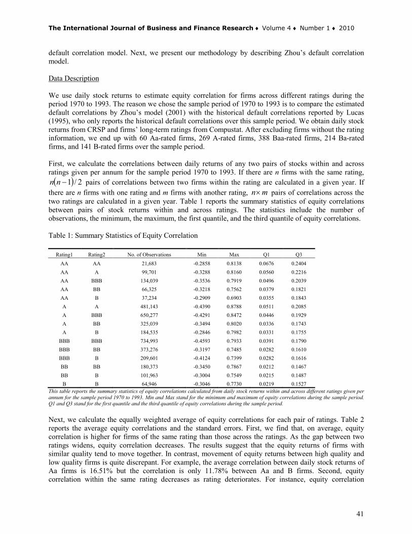
( ) 2/1−nn pairs of correlations between two firms within the rating are calculated in a given year. If there are n firms with one rating and m firms with another rating, n m× pairs of correlations across the two ratings are calculated in a given year. Table 1 reports the summary statistics of equity correlations between pairs of stock returns within and across ratings. The statistics include the number of observations, the minimum, the maximum, the first quantile, and the third quantile of equity correlations. Table 1: Summary Statistics of Equity Correlation

Rating1 Rating2 No. of Observations Min Max Q1 Q3 AA AA 21,683 -0.2858 0.8138 0.0676 0.2404 AA A 99,701 -0.3288 0.8160 0.0560 0.2216 AA BBB 134,039 -0.3536 0.7919 0.0496 0.2039 AA BB 66,325 -0.3218 0.7562 0.0379 0.1821 AA B 37,234 -0.2909 0.6903 0.0355 0.1843 A A 481,143 -0.4390 0.8788 0.0511 0.2085 A BBB 650,277 -0.4291 0.8472 0.0446 0.1929 A BB 325,039 -0.3494 0.8020 0.0336 0.1743 A B 184,535 -0.2846 0.7982 0.0331 0.1755

BBB BBB 734,993 -0.4593 0.7933 0.0391 0.1790 BBB BB 373,276 -0.3197 0.7485 0.0282 0.1610 BBB B 209,601 -0.4124 0.7399 0.0282 0.1616 BB BB 180,373 -0.3450 0.7867 0.0212 0.1467 BB B 101,963 -0.3004 0.7549 0.0215 0.1487 B B 64,946 -0.3046 0.7730 0.0219 0.1527

This table reports the summary statistics of equity correlations calculated from daily stock returns within and across different ratings given per annum for the sample period 1970 to 1993. Min and Max stand for the minimum and maximum of equity correlations during the sample period. Q1 and Q3 stand for the first quantile and the third quantile of equity correlations during the sample period. Next, we calculate the equally weighted average of equity correlations for each pair of ratings. Table 2 reports the average equity correlations and the standard errors. First, we find that, on average, equity correlation is higher for firms of the same rating than those across the ratings. As the gap between two ratings widens, equity correlation decreases. The results suggest that the equity returns of firms with similar quality tend to move together. In contrast, movement of equity returns between high quality and low quality firms is quite discrepant. For example, the average correlation between daily stock returns of Aa firms is 16.51% but the correlation is only 11.78% between Aa and B firms. Second, equity correlation within the same rating decreases as rating deteriorates. For instance, equity correlation

41


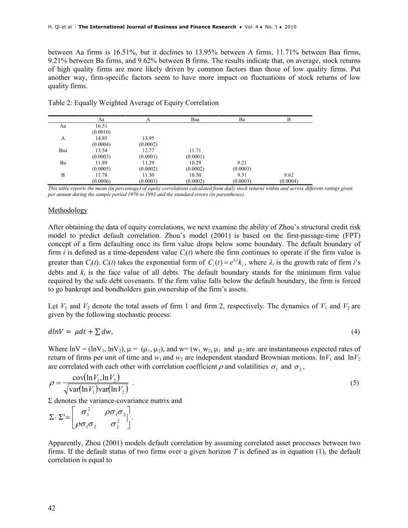
between Aa firms is 16.51%, but it declines to 13.95% between A firms, 11.71% between Baa firms, 9.21% between Ba firms, and 9.62% between B firms. The results indicate that, on average, stock returns of high quality firms are more likely driven by common factors than those of low quality firms. Put another way, firm-specific factors seem to have more impact on fluctuations of stock returns of low quality firms. Table 2: Equally Weighted Average of Equity Correlation

Aa A Baa Ba B Aa 16.51

(0.0010)

A 14.85 (0.0004)

13.95 (0.0002)

Baa 13.54 (0.0003)

12.77 (0.0001)

11.71 (0.0001)

Ba 11.89 (0.0005)

11.29 (0.0002)

10.29 (0.0002)

9.21 (0.0003)

B 11.78 (0.0006)

11.30 (0.0003)

10.30 (0.0002)

9.31 (0.0003)

9.62 (0.0004)

This table reports the mean (in percentage) of equity correlations calculated from daily stock returns within and across different ratings given per annum during the sample period 1970 to 1993 and the standard errors (in parentheses). Methodology After obtaining the data of equity correlations, we next examine the ability of Zhou’s structural credit risk model to predict default correlation. Zhou’s model (2001) is based on the first-passage-time (FPT) concept of a firm defaulting once its firm value drops below some boundary. The default boundary of firm i is defined as a time-dependent value Ci(t) where the firm continues to operate if the firm value is greater than Ci(t). Ci(t) takes the exponential form of ( ) it

i iC t e kλ= , where λi is the growth rate of firm i’s debts and ki is the face value of all debts. The default boundary stands for the minimum firm value required by the safe debt covenants. If the firm value falls below the default boundary, the firm is forced to go bankrupt and bondholders gain ownership of the firm’s assets. Let V1 and V2 denote the total assets of firm 1 and firm 2, respectively. The dynamics of V1 and V2 are given by the following stochastic process: 𝑑𝑑𝑑𝑑𝑑𝑑𝑑𝑑 = 𝜇𝜇𝑑𝑑𝜇𝜇 + ∑𝑑𝑑𝑑𝑑, (4) Where lnV = (lnV1, lnV2), µ = (µ1, µ2), and w= (w1, w2). µ1 and µ2 are are instantaneous expected rates of return of firms per unit of time and w1 and w2 are independent standard Brownian motions. lnV1 and lnV2

are correlated with each other with correlation coefficient ρ and volatilities 1σ and 2σ , ( )

( ) ( )21

21

lnvarlnvarln,lncov

VVVV

=ρ . (5)

Σ denotes the variance-covariance matrix and

=⋅ 2

221

2121'ΣΣ

σσρσσρσσ

.

Apparently, Zhou (2001) models default correlation by assuming correlated asset processes between two firms. If the default status of two firms over a given horizon T is defined as in equation (1), the default correlation is equal to

42


[ ] [ ] [ ][ ] [ ]

1 2 1 2

1

( ) ( ) ( ) ( )

( ) 2 ()D

E T T E T E T

Var T Var T

ω ϖ ω ωρ

ω ω

⋅ −= . (6)

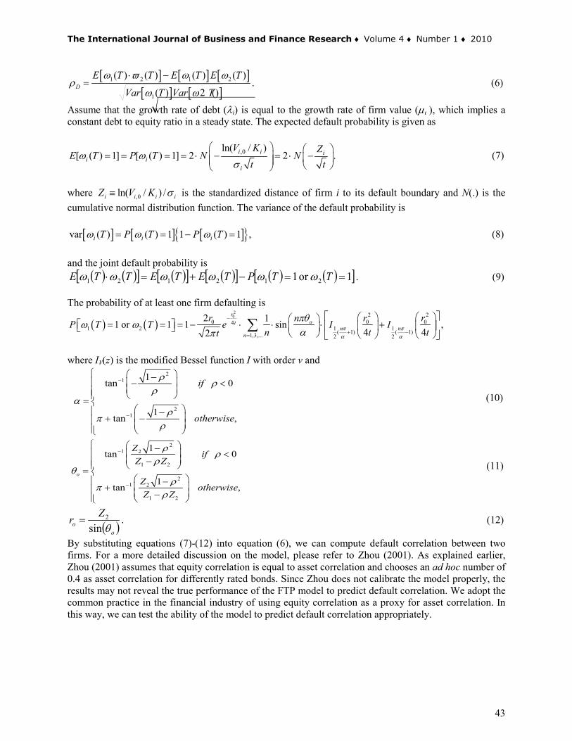
Assume that the growth rate of debt (λi) is equal to the growth rate of firm value (µι ), which implies a constant debt to equity ratio in a steady state. The expected default probability is given as

,0ln( / )[ ( ) 1] [ ( ) 1] 2 2 .i i i

i ii

V K ZE T P T N Nt t

ω ωσ

= = = = ⋅ − = ⋅ −

(7)

where ,0ln( / ) /i i i iZ V K σ≡ is the standardized distance of firm i to its default boundary and N(.) is the cumulative normal distribution function. The variance of the default probability is

[ ] [ ] [ ]{ }var ( ) ( ) 1 1 ( ) 1 ,i i iT P T P Tω ω ω= = − = (8) and the joint default probability is

( ) ( )[ ] ( )[ ] ( )[ ] ( ) ( )[ ]1or 1 212121 ==−+=⋅ TTPTETETTE ωωωωωω . (9) The probability of at least one firm defaulting is

( ) ( )2

0 2 20 0 04

1 2 1 1( 1) ( 1)1,3,... 2 2

2 11 or 1 1 sin ,4 42

rot

n nn

r n r rP T T e I In t tt π π

α α

πθω ω

απ

−

+ −=

= = = − ⋅ ⋅ ⋅ + ∑

where IV(z) is the modified Bessel function I with order v and

21

21

1tan 0

1tan ,

if

otherwise

ρρ

ρα

ρπ

ρ

−

−

− − < =

− + −

(10)

21 2

1 2

21 2

1 2

1tan 0

1tan ,

o

Zif

Z Z

Zotherwise

Z Z

ρρ

ρθ

ρπ

ρ

−

−

− < − =

− + −

(11)

( )oo

Zrθsin2= . (12)

By substituting equations (7)-(12) into equation (6), we can compute default correlation between two firms. For a more detailed discussion on the model, please refer to Zhou (2001). As explained earlier, Zhou (2001) assumes that equity correlation is equal to asset correlation and chooses an ad hoc number of 0.4 as asset correlation for differently rated bonds. Since Zhou does not calibrate the model properly, the results may not reveal the true performance of the FTP model to predict default correlation. We adopt the common practice in the financial industry of using equity correlation as a proxy for asset correlation. In this way, we can test the ability of the model to predict default correlation appropriately.

43


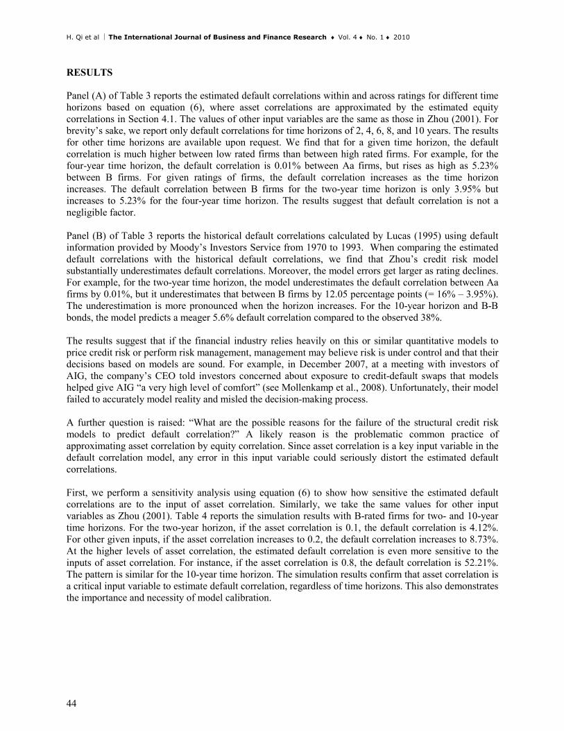
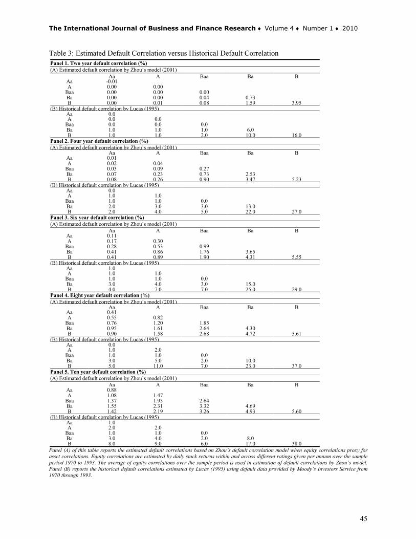
RESULTS Panel (A) of Table 3 reports the estimated default correlations within and across ratings for different time horizons based on equation (6), where asset correlations are approximated by the estimated equity correlations in Section 4.1. The values of other input variables are the same as those in Zhou (2001). For brevity’s sake, we report only default correlations for time horizons of 2, 4, 6, 8, and 10 years. The results for other time horizons are available upon request. We find that for a given time horizon, the default correlation is much higher between low rated firms than between high rated firms. For example, for the four-year time horizon, the default correlation is 0.01% between Aa firms, but rises as high as 5.23% between B firms. For given ratings of firms, the default correlation increases as the time horizon increases. The default correlation between B firms for the two-year time horizon is only 3.95% but increases to 5.23% for the four-year time horizon. The results suggest that default correlation is not a negligible factor. Panel (B) of Table 3 reports the historical default correlations calculated by Lucas (1995) using default information provided by Moody’s Investors Service from 1970 to 1993. When comparing the estimated default correlations with the historical default correlations, we find that Zhou’s credit risk model substantially underestimates default correlations. Moreover, the model errors get larger as rating declines. For example, for the two-year time horizon, the model underestimates the default correlation between Aa firms by 0.01%, but it underestimates that between B firms by 12.05 percentage points (= 16% – 3.95%). The underestimation is more pronounced when the horizon increases. For the 10-year horizon and B-B bonds, the model predicts a meager 5.6% default correlation compared to the observed 38%. The results suggest that if the financial industry relies heavily on this or similar quantitative models to price credit risk or perform risk management, management may believe risk is under control and that their decisions based on models are sound. For example, in December 2007, at a meeting with investors of AIG, the company’s CEO told investors concerned about exposure to credit-default swaps that models helped give AIG “a very high level of comfort” (see Mollenkamp et al., 2008). Unfortunately, their model failed to accurately model reality and misled the decision-making process. A further question is raised: “What are the possible reasons for the failure of the structural credit risk models to predict default correlation?” A likely reason is the problematic common practice of approximating asset correlation by equity correlation. Since asset correlation is a key input variable in the default correlation model, any error in this input variable could seriously distort the estimated default correlations. First, we perform a sensitivity analysis using equation (6) to show how sensitive the estimated default correlations are to the input of asset correlation. Similarly, we take the same values for other input variables as Zhou (2001). Table 4 reports the simulation results with B-rated firms for two- and 10-year time horizons. For the two-year horizon, if the asset correlation is 0.1, the default correlation is 4.12%. For other given inputs, if the asset correlation increases to 0.2, the default correlation increases to 8.73%. At the higher levels of asset correlation, the estimated default correlation is even more sensitive to the inputs of asset correlation. For instance, if the asset correlation is 0.8, the default correlation is 52.21%. The pattern is similar for the 10-year time horizon. The simulation results confirm that asset correlation is a critical input variable to estimate default correlation, regardless of time horizons. This also demonstrates the importance and necessity of model calibration.

44


Table 3: Estimated Default Correlation versus Historical Default Correlation

Panel 1. Two year default correlation (%) (A) Estimated default correlation by Zhou’s model (2001)

Aa A Baa Ba B Aa -0.01 A 0.00 0.00

Baa 0.00 0.00 0.00 Ba 0.00 0.00 0.04 0.73 B 0.00 0.01 0.08 1.59 3.95

(B) Historical default correlation by Lucas (1995) Aa 0.0 A 0.0 0.0

Baa 0.0 0.0 0.0 Ba 1.0 1.0 1.0 6.0 B 1.0 1.0 2.0 10.0 16.0

Panel 2. Four year default correlation (%) (A) Estimated default correlation by Zhou’s model (2001)

Aa A Baa Ba B Aa 0.01 A 0.02 0.04

Baa 0.03 0.09 0.27 Ba 0.07 0.23 0.73 2.53 B 0.08 0.26 0.90 3.47 5.23


Baa 1.0 1.0 0.0 Ba 2.0 3.0 3.0 13.0 B 2.0 4.0 5.0 22.0 27.0

Panel 3. Six year default correlation (%) (A) Estimated default correlation by Zhou’s model (2001)

Aa A Baa Ba B Aa 0.11 A 0.17 0.30

Baa 0.28 0.53 0.99 Ba 0.41 0.86 1.76 3.65 B 0.41 0.89 1.90 4.31 5.55


Baa 1.0 1.0 0.0 Ba 3.0 4.0 3.0 15.0 B 4.0 7.0 7.0 25.0 29.0

Panel 4. Eight year default correlation (%) (A) Estimated default correlation by Zhou’s model (2001)

Aa A Baa Ba B Aa 0.41 A 0.55 0.82

Baa 0.76 1.20 1.85 Ba 0.95 1.61 2.64 4.30 B 0.90 1.58 2.68 4.72 5.61


Baa 1.0 1.0 0.0 Ba 3.0 5.0 2.0 10.0 B 5.0 11.0 7.0 23.0 37.0

Panel 5. Ten year default correlation (%) (A) Estimated default correlation by Zhou’s model (2001)

Aa A Baa Ba B Aa 0.88 A 1.08 1.47

Baa 1.37 1.93 2.64 Ba 1.55 2.31 3.32 4.69 B 1.42 2.19 3.26 4.93 5.60


Baa 1.0 1.0 0.0 Ba 3.0 4.0 2.0 8.0 B 8.0 9.0 6.0 17.0 38.0

Panel (A) of this table reports the estimated default correlations based on Zhou’s default correlation model when equity correlations proxy for asset correlations. Equity correlations are estimated by daily stock returns within and across different ratings given per annum over the sample period 1970 to 1993. The average of equity correlations over the sample period is used in estimation of default correlations by Zhou’s model. Panel (B) reports the historical default correlations estimated by Lucas (1995) using default data provided by Moody’s Investors Service from 1970 through 1993.

45


Table 4: Sensitivity of Model-predicted Default Correlation to Asset Correlation

Panel 1. Two year asset correlation vs. default correlation Asset Correlation 0.1 0.2 0.3 0.4 0.5 0.6 0.7 0.8 0.9 Default Correlation (%) 4.12 8.73 13.87 19.62 26.06 33.39 41.9 52.21 65.93 Panel 2. Ten year asset correlation vs. default correlation Asset Correlation 0.1 0.2 0.3 0.4 0.5 0.6 0.7 0.8 0.9 Default Correlation (%) 5.82 11.77 17.93 24.37 31.22 38.65 46.94 56.66 69.23

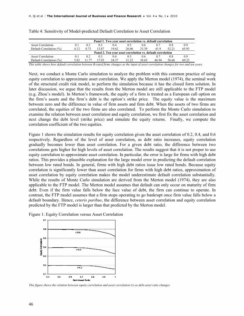
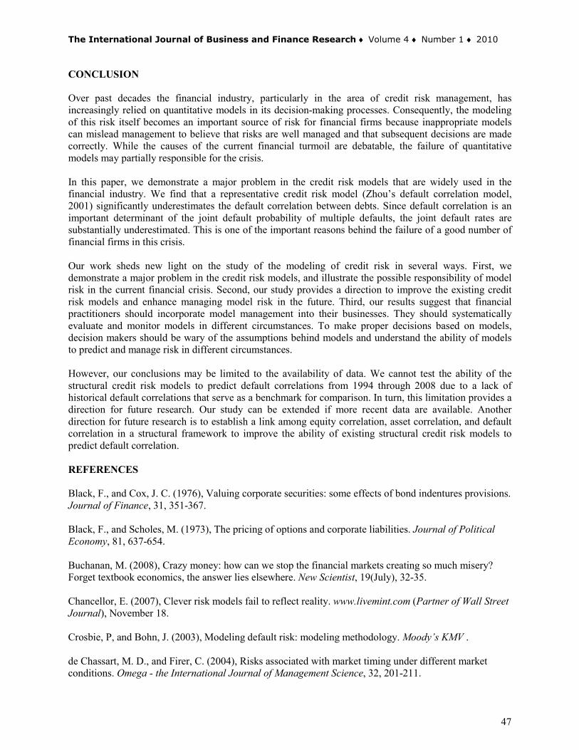
This table shows how default correlation between B-rated firms changes as the input of asset correlation changes for two and ten years. Next, we conduct a Monte Carlo simulation to analyze the problem with this common practice of using equity correlation to approximate asset correlation. We apply the Merton model (1974), the seminal work of the structural credit risk model, to perform the simulation because it has the closed form solution. In later discussion, we argue that the results from the Merton model are still applicable to the FTP model (e.g. Zhou’s model). In Merton’s framework, the equity of a firm is treated as a European call option on the firm’s assets and the firm’s debt is the option’s strike price. The equity value is the maximum between zero and the difference in value of firm assets and firm debt. When the assets of two firms are correlated, the equities of the two firms are also correlated. To perform the Monte Carlo simulation to examine the relation between asset correlation and equity correlation, we first fix the asset correlation and next change the debt level (strike price) and simulate the equity returns. Finally, we compute the correlation coefficient of the two equities. Figure 1 shows the simulation results for equity correlation given the asset correlation of 0.2, 0.4, and 0.6 respectively. Regardless of the level of asset correlation, as debt ratio increases, equity correlation gradually becomes lower than asset correlation. For a given debt ratio, the difference between two correlations gets higher for high levels of asset correlation. The results suggest that it is not proper to use equity correlation to approximate asset correlation. In particular, the error is large for firms with high debt ratios. This provides a plausible explanation for the large model error in predicting the default correlation between low rated bonds. In general, firms with high debt ratios issue low rated bonds. Because equity correlation is significantly lower than asset correlation for firms with high debt ratios, approximation of asset correlation by equity correlation makes the model underestimate default correlation substantially. While the results of Monte Carlo simulation are derived from the Merton model (1974), they are also applicable to the FTP model. The Merton model assumes that default can only occur on maturity of firm debt. Even if the firm value falls below the face value of debt, the firm can continue to operate. In contrast, the FTP model assumes that a firm stops operating to go bankrupt once firm value falls below a default boundary. Hence, ceteris paribus, the difference between asset correlation and equity correlation predicted by the FTP model is larger than that predicted by the Merton model.

Figure 1: Equity Correlation versus Asset Correlation

This figure shows the relation between equity correlation and asset correlation (r) as debt-asset ratio changes.

46


CONCLUSION Over past decades the financial industry, particularly in the area of credit risk management, has increasingly relied on quantitative models in its decision-making processes. Consequently, the modeling of this risk itself becomes an important source of risk for financial firms because inappropriate models can mislead management to believe that risks are well managed and that subsequent decisions are made correctly. While the causes of the current financial turmoil are debatable, the failure of quantitative models may partially responsible for the crisis. In this paper, we demonstrate a major problem in the credit risk models that are widely used in the financial industry. We find that a representative credit risk model (Zhou’s default correlation model, 2001) significantly underestimates the default correlation between debts. Since default correlation is an important determinant of the joint default probability of multiple defaults, the joint default rates are substantially underestimated. This is one of the important reasons behind the failure of a good number of financial firms in this crisis. Our work sheds new light on the study of the modeling of credit risk in several ways. First, we demonstrate a major problem in the credit risk models, and illustrate the possible responsibility of model risk in the current financial crisis. Second, our study provides a direction to improve the existing credit risk models and enhance managing model risk in the future. Third, our results suggest that financial practitioners should incorporate model management into their businesses. They should systematically evaluate and monitor models in different circumstances. To make proper decisions based on models, decision makers should be wary of the assumptions behind models and understand the ability of models to predict and manage risk in different circumstances. However, our conclusions may be limited to the availability of data. We cannot test the ability of the structural credit risk models to predict default correlations from 1994 through 2008 due to a lack of historical default correlations that serve as a benchmark for comparison. In turn, this limitation provides a direction for future research. Our study can be extended if more recent data are available. Another direction for future research is to establish a link among equity correlation, asset correlation, and default correlation in a structural framework to improve the ability of existing structural credit risk models to predict default correlation. REFERENCES Black, F., and Cox, J. C. (1976), Valuing corporate securities: some effects of bond indentures provisions. Journal of Finance, 31, 351-367. Black, F., and Scholes, M. (1973), The pricing of options and corporate liabilities. Journal of Political Economy, 81, 637-654. Buchanan, M. (2008), Crazy money: how can we stop the financial markets creating so much misery? Forget textbook economics, the answer lies elsewhere. New Scientist, 19(July), 32-35. Chancellor, E. (2007), Clever risk models fail to reflect reality. www.livemint.com (Partner of Wall Street Journal), November 18. Crosbie, P, and Bohn, J. (2003), Modeling default risk: modeling methodology. Moody’s KMV . de Chassart, M. D., and Firer, C. (2004), Risks associated with market timing under different market conditions. Omega - the International Journal of Management Science, 32, 201-211.

47


DerivativeFitch (2004), Default VECTOR 3.1 model user manual. Duffie, D., and Singleton, K. J. (1997), An econometric model of the term structure of interest rate swap yields. Journal of Finance, 52, 1287-1321. Duffie, D., and Singleton, K. J. (1999), Modeling term structure of defaultable bonds. Review of Financial Studies, 12, 687-720. Giesecke, K. (2003), Successive correlated defaults: pricing trends and simulation. Working Paper, Cornell University. Giesecke, K. (2006), Default and information. Journal of Economic Dynamics and Control, 30, 2281-2303. Gupton, G. M., Finger, C. C., and Bhatia, M. (1997), CreditMetricsTM – Technical documents. J.P. Morgan New York. Jameson, B. (2008), The blunders that led to catastrophe. New Scientist, 27(September), 8-9. Jarrow, R., Lando, D., and Turnbull, S. (1997), A Markov model for the term structure of credit risk spreads. Review of Financial Studies, 10, 481-523. Jarrow, R, and Turnbull, S. (1995), Pricing options on financial securities subject to default risk. Journal of Finance, 50, 53-86. Lando, D. (1998), On Cox process and credit risky securities. Review of Derivatives Research, 2, 99-120. Lohr, S. (2008), In modeling risk, the human factor was left out. The New York Times, November 5. Lucas, D. J. (1995), Default correlation and credit analysis. Journal of Fixed Income, 4, 76-87. Madan, D., and Unal, H. (1998), Pricing the risks of default. Review of Derivatives Research, 2, 121-160. Madan, D., and Unal, H. (2000), Pricing risky debt: a two-factor hazard-rate model with complex capital structure. Journal of Financial and Quantitative Analysis, 35, 43-65. Merton, R. C. (1974), On the pricing of corporate debts: the risk structure of interest rates. Journal of Finance, 29, 449-470. Mollenkamp, C., Ng, S., Pleven, L., and Smith, R. (2008), Behind AIG’s fall, risk models failed to pass real-world test. Wall Street Journal, November 3, A.1. Zhou, C. (2001), An analysis of default correlations and multiple defaults. The Review of Financial Studies, 14, 555-576.

BIOGRAPHY Dr. Howard Qi is an Assistant Professor of Finance at Michigan Tech University, He can be contacted at: School of Business and Economics, Michigan Tech University, 1400 Townsend Drive, Houghton, MI 49931, US. Email: [email protected]

48


Dr. Yan Alice Xie is an Assistant Professor of Finance at University of Michigan-Dearborn, She can be contacted at: School of Management, University of Michigan-Dearborn, 19000 Hubbard Drive, Dearborn, MI 48126, US. Email: [email protected] Dr. Sheen Liu is an Assistant Professor of Finance at Washington State University – Vancouver, He can be contacted at: Department of Finance, Insurance, and Real Estate, 14204 NE Salmon Creek Avenue, Vancouver, WA 98686, US. Email: [email protected]

49

Documents

Credit risk models: An analysis of default correlation