Embed Size (px)
Citation preview
Prologue Ghosh et. al. Firms and Financial Markets Model Aniket (2006b) Burgess & Pande (2003) Epilogue
Credit, Saving and Insurance
EC307 ECONOMIC DEVELOPMENT
Dr. Kumar Aniket
University of Cambridge & LSE Summer School
Lecture 8
created on June 6, 2010
c©Kumar Aniket
Prologue Ghosh et. al. Firms and Financial Markets Model Aniket (2006b) Burgess & Pande (2003) Epilogue
READINGS
Tables and figures in this lecture are taken from:
Chapters 14 of Ray (1998)
Ghosh, P., Mookherjee, D., & Ray, D, (2000). Credit Rationing in
Developing Countries: An Overview of the Theory. Mimeo.
Aniket, K. (2006). Does Subsidising the Cost of Capital Really
Help the Poorest? An Analysis of Saving Opportunities in Group
Lending. ESE Discussion Paper.
Burgess, R. and Pande, R. (2003). Do Rural Banks Matter?:
Evidence from the Indian Social Banking Experiment. STICERD,
LSE.
◮ Class based on Burgess, R., and R. Pande (2005). Do rural banks
matter?: Evidence from the Indian social banking experiment.
American economic review 95, no. 3: 780-795.
c©Kumar Aniket
Prologue Ghosh et. al. Firms and Financial Markets Model Aniket (2006b) Burgess & Pande (2003) Epilogue
WHY IS ACCESS TO FINANCE IMPORTANT?
◦ Finance the shortfalls in consumption – consumption smoothing
◦ Finance ongoing production – expand production opportunities
◦ Appropriate public policy response to this is complicated by the
fact that the extent of credit rationing in such situations /
countries may be endogenously determined – informational and
enforcement problems as opposed to lack of funds may underlie credit
rationing
◦ If financial institutions don’t have full information about the
riskiness of projects that individuals plan to undertake, they may
ration credit as a means of ensuring that citizens undertake less
risky projects
c©Kumar Aniket
Prologue Ghosh et. al. Firms and Financial Markets Model Aniket (2006b) Burgess & Pande (2003) Epilogue
INFORMAL FINANCIAL INSTITUTIONS
Informal financial institutions may be better at dealing with
informational and enforcement problems
◦ They may be able to use social sanctions to guarantee loans as
opposed to collateral requirements
◦ allowing poor (who would otherwise be screened out of credit
market due to inability to comply with collateral and other
requirements) to gain access to credit
⇒ credit deepening – work because they deal with informational
problems which confound formal credit markets.
c©Kumar Aniket
Prologue Ghosh et. al. Firms and Financial Markets Model Aniket (2006b) Burgess & Pande (2003) Epilogue
WHY INTERVENE IN CREDIT MARKETS: MARKET
FAILURE
Market for loans – occurs between those who are willing to postpone
consumption and those wanting to make investments / prepone
consumption – determines price of credit (interest rate)
Market failure – competitive market fails to bring about an efficient
allocation of credit – outcome is not Pareto efficient, i.e., not possible
to make someone better off without making someone worse off
Generating trade in loans via introduction of credit market – should
lead to Pareto improvements relative to autarky
First fundamental welfare theorem: competitive markets without
externalities generate a Pareto efficient outcome
but in developing countries, problem of repayment may lead to
deviations from this benchmark – unable to pay or unwilling to pay
c©Kumar Aniket
Prologue Ghosh et. al. Firms and Financial Markets Model Aniket (2006b) Burgess & Pande (2003) Epilogue
◦ If enforcement costs too high – lender may be unwilling to lend to
high risks – typically poor people – poor get rationed out of
formal credit market and may have to rely on informal market
where terms are much worse (evil moneylender etc.)
◦ Credit markets may also diverge from idealised market because
of informational problems – problems with monitoring
borrowers – may not know how reliable borrower is and how
wisely they will use funds – again, this leads to some individuals
being rationed out of the market or being offered smaller loans
relative to where monitoring was costless
c©Kumar Aniket
Prologue Ghosh et. al. Firms and Financial Markets Model Aniket (2006b) Burgess & Pande (2003) Epilogue
CREDIT RATIONING IN DEVELOPING COUNTRIES
Stylised facts about rural credit markets from various case studies
and empirical work.
1. Loans advanced on basis of oral agreements rather than written
one
2. No or very little collateral, making default a feasible option
3. Credit markets highly segmented, marked with long term
exclusive relationships and repeat lending
c©Kumar Aniket
Prologue Ghosh et. al. Firms and Financial Markets Model Aniket (2006b) Burgess & Pande (2003) Epilogue
1. Interest rates higher on average than bank interest rate with
significant dispersion presenting arbitrage opportunities
2. Frequent inter-linkage with other markets, such as land, labour
or crop
3. Significant credit rationing, whereby
– borrowers are unable to borrow all they want (micro credit
rationing)
– or some applicants are unable to borrow at all (macro credit
rationing)
c©Kumar Aniket
Prologue Ghosh et. al. Firms and Financial Markets Model Aniket (2006b) Burgess & Pande (2003) Epilogue
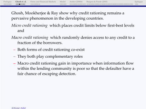
Ghosh, Mookherjee & Ray show why credit rationing remains a
pervasive phenomenon in the developing countries.
Micro credit rationing which places credit limits below first-best levels
and
Macro credit rationing which randomly denies access to any credit to a
fraction of the borrowers.
– Both forms of credit rationing co-exist
– They both play complementary roles
– Macro credit rationing gain in importance when information flow
within the lending community is poor so that the defaulter have a
fair chance of escaping detection.
c©Kumar Aniket
Prologue Ghosh et. al. Firms and Financial Markets Model Aniket (2006b) Burgess & Pande (2003) Epilogue
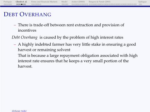
DEBT OVERHANG
– There is trade-off between rent extraction and provision of
incentives
Debt Overhang is caused by the problem of high interest rates
– A highly indebted farmer has very little stake in ensuring a good
harvest or remaining solvent
That is because a large repayment obligation associated with high
interest rate ensures that he keeps a very small portion of the
harvest.
c©Kumar Aniket

Prologue Ghosh et. al. Firms and Financial Markets Model Aniket (2006b) Burgess & Pande (2003) Epilogue
– Keeping this in mind the lender may be reluctant to raise the
interest rate beyond a certain point
– Volume of credit and effort level in this credit market would be
less than first best
– Borrowers with greater wealth or collateral can obtain cheaper
credit, work harder and earn more income as a result
◦ Existing asset inequalities within the borrowing class are
projected and possibly magnified by the operation of the credit
market causing persistence of poverty. (Recall the parallel Galor
and Zeira argument that led to a similar result)
c©Kumar Aniket

Prologue Ghosh et. al. Firms and Financial Markets Model Aniket (2006b) Burgess & Pande (2003) Epilogue
LESSONS
– Distribution of power across lenders and borrowers has a strong
implication for the degree of credit rationing, effort levels and
efficiency
Greater bargaining power to the lender reduces available credit
and efficiency
– Rent extraction motives can run counter to the surplus
maximization objectives beyond a point
– Social policies that empower the borrower and increase his
bargaining strength are lively to increase efficiency
c©Kumar Aniket
Prologue Ghosh et. al. Firms and Financial Markets Model Aniket (2006b) Burgess & Pande (2003) Epilogue
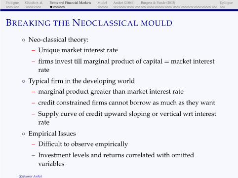
BREAKING THE NEOCLASSICAL MOULD
◦ Neo-classical theory:
– Unique market interest rate
– firms invest till marginal product of capital = market interest
rate
◦ Typical firm in the developing world
– marginal product greater than market interest rate
– credit constrained firms cannot borrow as much as they want
– Supply curve of credit upward sloping or vertical wrt interest
rate
◦ Empirical Issues
– Difficult to observe empirically
– Investment levels and returns correlated with omitted
variables
c©Kumar Aniket
Prologue Ghosh et. al. Firms and Financial Markets Model Aniket (2006b) Burgess & Pande (2003) Epilogue
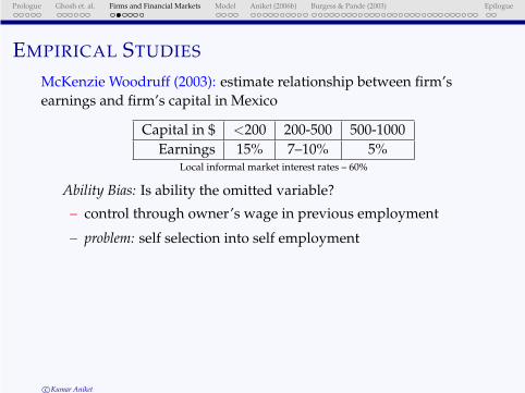
EMPIRICAL STUDIES
McKenzie Woodruff (2003): estimate relationship between firm’s
earnings and firm’s capital in Mexico
Capital in $ <200 200-500 500-1000
Earnings 15% 7–10% 5%Local informal market interest rates – 60%
Ability Bias: Is ability the omitted variable?
– control through owner’s wage in previous employment
– problem: self selection into self employment
c©Kumar Aniket
Prologue Ghosh et. al. Firms and Financial Markets Model Aniket (2006b) Burgess & Pande (2003) Epilogue
Goldstein Udry (1999)
Returns from switching from maize, cassava to pineapple
estimated at 1200%!
Very few people grow pineapple
– unobserved heterogeneity between people who have switched
others who have not
c©Kumar Aniket

Prologue Ghosh et. al. Firms and Financial Markets Model Aniket (2006b) Burgess & Pande (2003) Epilogue
Fazzari et. al. (1988): cash flow has a positive effect on firm’s
investment
Cash flows could proxy for productivity shocks
– control for firms’s market value to eliminate productivity
shocks
– problem: market may not know everything about firm’s
productivity
Lamont (1997): effect of cash flow shock from unidentifiable source
shock to the price of crude
Looks at non-oil investment of companies that own an oil
company in reaction to an oil price shock
– a strong cash flow effect
– managerial behaviour in response to “free cash flow”
c©Kumar Aniket
Prologue Ghosh et. al. Firms and Financial Markets Model Aniket (2006b) Burgess & Pande (2003) Epilogue
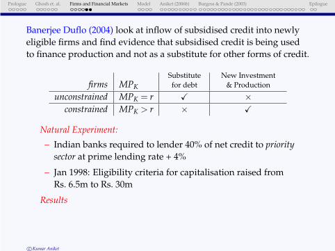
Banerjee Duflo (2004) look at inflow of subsidised credit into newly
eligible firms and find evidence that subsidised credit is being used
to finance production and not as a substitute for other forms of credit.
firms MPK
Substitute
for debt
New Investment
& Production
unconstrained MPK = r X ×
constrained MPK > r × X
Natural Experiment:
– Indian banks required to lender 40% of net credit to priority
sector at prime lending rate + 4%
– Jan 1998: Eligibility criteria for capitalisation raised from
Rs. 6.5m to Rs. 30m
Results
c©Kumar Aniket
Prologue Ghosh et. al. Firms and Financial Markets Model Aniket (2006b) Burgess & Pande (2003) Epilogue
– Bank lending and firms revenues went up for the newly
eligible firms relative to old firms implying subsided credit
was used to finance production
– no evidence of substitution of bank credit for borrowing from
the market
– many firms severely credit constrained with high MPK
c©Kumar Aniket
Prologue Ghosh et. al. Firms and Financial Markets Model Aniket (2006b) Burgess & Pande (2003) Epilogue
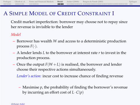
A SIMPLE MODEL OF CREDIT CONSTRAINT I
Credit market imperfection: borrower may choose not to repay since
her revenue is invisible to the lender
Model
– Borrower has wealth W and access to a deterministic production
process F(·).
– A lender lends L to the borrower at interest rate r to invest in the
production process.
– Once the output F(W +L) is realised, the borrower and lender
choose their respective actions simultaneously.
Lender’s action: incur cost to increase chance of finding revenue
– Maximise p, the probability of finding the borrower’s revenue
by incurring an effort cost of L ·C(p)
c©Kumar Aniket
Prologue Ghosh et. al. Firms and Financial Markets Model Aniket (2006b) Burgess & Pande (2003) Epilogue
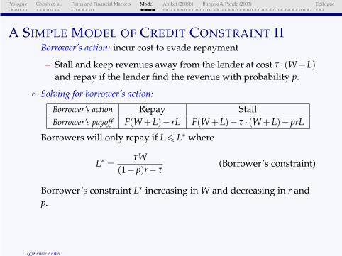
A SIMPLE MODEL OF CREDIT CONSTRAINT IIBorrower’s action: incur cost to evade repayment
– Stall and keep revenues away from the lender at cost τ · (W +L)
and repay if the lender find the revenue with probability p.
◦ Solving for borrower’s action:
Borrower’s action Repay Stall
Borrower’s payoff F(W +L)− rL F(W +L)− τ · (W +L)−prL
Borrowers will only repay if L 6 L∗ where
L∗ =τW
(1−p)r− τ(Borrower’s constraint)
Borrower’s constraint L∗ increasing in W and decreasing in r and
p.
c©Kumar Aniket

Prologue Ghosh et. al. Firms and Financial Markets Model Aniket (2006b) Burgess & Pande (2003) Epilogue
A SIMPLE MODEL OF CREDIT CONSTRAINT III◦ Solving for lender’s action
Let C(p) = −c ln1−p which implies that C(0) = 0, C(1) = ∞ and C′(p) > 0. Lender’s
total cost of finding revenue is convex and increasing in p.
The lender’s net benefit given by:
rPL− (−c ln(1−p) ·L)
To find the optimal choice of p, differentiate the above expression and equate to 0.
The optimal choice of p is such that:
r(1−p) = c (Optimal p)
By substituting Optimal p in Borrower’s constraint, we obtain the following:
L∗
W=
1(
cτ)
−1= µ (Final Constraint)
c©Kumar Aniket
Prologue Ghosh et. al. Firms and Financial Markets Model Aniket (2006b) Burgess & Pande (2003) Epilogue
A SIMPLE MODEL OF CREDIT CONSTRAINT IVResult
µ determines the multiple of the borrower’s wealth that she can
borrow.
– µ is increasing in τ , the cost of stalling the lender, and
decreasing in c, the lender’s cost of finding the borrower’s
revenue.
µ is increasing in the ratio τc , the measure of the economy’s
financial development.
– As the economy develops financially, borrower’s are less credit
constrained.
c©Kumar Aniket

Prologue Ghosh et. al. Firms and Financial Markets Model Aniket (2006b) Burgess & Pande (2003) Epilogue
WEALTH
Microfinance lenders across the world require that borrowerrepay much before the completion of the project
Periodicity: Frequency of loan repayment
Periodicity used by microfinance institutions to compensate for
lack of collateral
Force borrower to acquire stake in their own projects
Borrower need to have some wealth to be able to borrow.
c©Kumar Aniket
Prologue Ghosh et. al. Firms and Financial Markets Model Aniket (2006b) Burgess & Pande (2003) Epilogue
SAVINGS
Poor have extremely volatile income streams
Require savings instruments to be able to
Smooth consumption
Self-insure
Save towards lumpy investments
Poor are offered no saving instruments in the rural credit market
Moneylender lends but does not take any saving deposits. Why?
Covariate Risks
Transaction Costs
How can Microfinance institutions help?
c©Kumar Aniket

Prologue Ghosh et. al. Firms and Financial Markets Model Aniket (2006b) Burgess & Pande (2003) Epilogue
CASESTUDY IN HARYANA, INDIA
⊙ Case-study of a Microfinance Institution in Harayana
Documents the innovative design features of India’s new national
microfinance programme.
◦ Lender offers saving opportunities
. . . by restricting loans to the group
. . . creates intra-group competition for loans
◦ Individuals can join a group as either a borrower or a saver
◦ Borrower partly self-finance’s the buffalo
◦ Saver co-finance’s the borrower’s project
. . . and gets a premium interest rate on her savings
⊙ We observed
• Intra-group income heterogeneity
• savers were poorer than borrowers
c©Kumar Aniket
Prologue Ghosh et. al. Firms and Financial Markets Model Aniket (2006b) Burgess & Pande (2003) Epilogue
ROLE OF SAVINGS IN MICROFINANCE: ANIKET 2006B
Offering saving opportunities in group lending would lead to
negative assortative matching along wealth lines:
Rich and poor match in the same group.
Could potentially initiate a chain where the poor who get
wealthier match with the other poor people and uplift them out
of poverty
c©Kumar Aniket
Prologue Ghosh et. al. Firms and Financial Markets Model Aniket (2006b) Burgess & Pande (2003) Epilogue
POVERTY TRAPS
without multiple market failures – marginal product of an individual
in an occupation should not reflect any endowment effects and hence
should not be explainable by parent’s wealth
However, even in developed countries – observe that credit market
constraints limit entry to entrepreneurial activities
⇒ endowments matter! – econometric evidence shows that wealthier
individuals more likely to become entrepreneur, not because they
have greater ability but because liquidity constraints bind less
strongly
Two reasons for this –
(a) use inherited wealth to finance fixed costs of setting up own
project
(b) use inherited wealth/assets as collateral to gain access to credit
markets to finance own project
c©Kumar Aniket

Prologue Ghosh et. al. Firms and Financial Markets Model Aniket (2006b) Burgess & Pande (2003) Epilogue
Poor in contrast –
(a) may have not inherited sufficient wealth to enable them to incur
fixed cost of taking on their own project
(b) may have not inherited sufficient wealth/assets to serve as
collateral to gain access to formal credit markets
Explain three things:
(i) persistence of inequality and poverty
(ii) why interventions which affect the distribution of endowments can have
large effects on welfare – possible to get rid of source of market failure
(iii) why lower inequality may be associated with higher growth – policies
which equalise opportunities across households may lead to
improvements in both equity and efficiency
c©Kumar Aniket

Prologue Ghosh et. al. Firms and Financial Markets Model Aniket (2006b) Burgess & Pande (2003) Epilogue
POSITIVE POLICIES
We are looking at a range of such opportunity enhancing policies
(e.g., land reform, microfinance, education, off-farm
diversification)
Only by affecting distribution of endowments can we get
permanent increases in welfare – tax/transfer mechanisms can
help households deal with crisis situations but if don’t change
distribution of endowments then no effects on permanent
income
c©Kumar Aniket

Prologue Ghosh et. al. Firms and Financial Markets Model Aniket (2006b) Burgess & Pande (2003) Epilogue
POSITIVE POLICIES
Idea of poverty traps being caused by market failure and the
importance of redistribution of opportunity in these contexts has
led to complete rethinking of design of public policy to affect
poverty and growth in developing countries – need more
empirical work to establish which policies work and which don’t
In the context of this lecture, if we believe that imperfections in
the credit market is a major factor behind why poor people stay
poor, then we have to ask ourselves, what can be done?
c©Kumar Aniket
Prologue Ghosh et. al. Firms and Financial Markets Model Aniket (2006b) Burgess & Pande (2003) Epilogue
SOCIAL BANKING
State interventions in credit markets are very common in less
developed countries. Are state-led credit programs useful in
encouraging growth and fighting poverty?
Pro: lack of access to credit limits ability of the poor in engaging in
productive activities and exiting poverty.
Con: Programs subject to elite capture and may actually worsen
terms for the poor in rural credit markets.
However, there have been limited evaluations of such programmes.
c©Kumar Aniket

Prologue Ghosh et. al. Firms and Financial Markets Model Aniket (2006b) Burgess & Pande (2003) Epilogue
STRUCTURAL CHANGE
Structural change: decline of agriculture . . .
– positive correlation with economic growth
– positive correlation with rising living standards
→ Key area of research in economic history, development
economics and macroeconomics (1950-70s)
. . . but most of the work is descriptive
→ We have a limited understanding of what drives structural
change especially at the micro level.
c©Kumar Aniket
Prologue Ghosh et. al. Firms and Financial Markets Model Aniket (2006b) Burgess & Pande (2003) Epilogue
Do Rural Banks Matter?: Evidence from the Indian Social
Banking Experiment
◦ The paper exploits the social banking experiment in India to
examine this issue carefully.
◦ Does the state-led expansion of commercial banks in rural areas
lead to structural change and engender economic growth?
◦ Does improved access to banks enable households to transform
their production activities?
◦ Idea that financial development may be a pre-requisite for
economic development influential in post-war Indian
governments
Social banking experiment in India motivated by the idea that lack
of access to bank was an impediment to modernisation and
industrialisation in rural areas, ie, structural change.
c©Kumar Aniket

Prologue Ghosh et. al. Firms and Financial Markets Model Aniket (2006b) Burgess & Pande (2003) Epilogue
BANK COMPANY ACQUISITION ACT, 1969
“The banking system touches the lives of millions and has to be
inspired by larger social purpose and has to subserve national
priorities and objectives such as rapid growth of agriculture,
small industries and exports, raising of employment levels,
encouragement of new entrepreneurs and development of
backward areas. For this purpose, it is necessary for the
government to take direct responsibility for the extension and
diversification of banking services and for the working of a
substantial part of the banking system”
c©Kumar Aniket
Prologue Ghosh et. al. Firms and Financial Markets Model Aniket (2006b) Burgess & Pande (2003) Epilogue
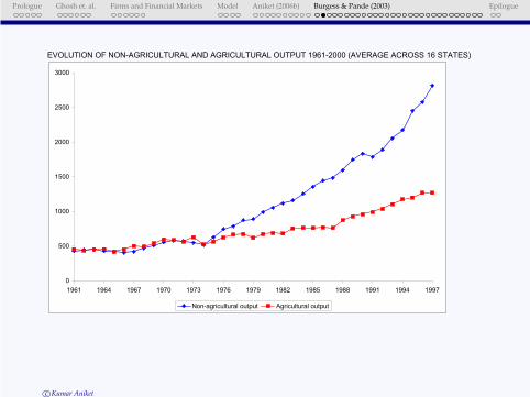
STRUCTURAL CHANGE IN INDIA
◦ Look at state domestic product data for 16 main states of India
over the period 1960-2000 – these 16 states account for over 95%
of Indian population
◦ Real agricultural output per capita relatively flat over period –
growth in agricultural output basically keeps track with growth
in population
◦ Real non-agricultural output per capita begins to diverge from
agricultural output around mid-1970s – but pattern highly
varied across states
c©Kumar Aniket
Prologue Ghosh et. al. Firms and Financial Markets Model Aniket (2006b) Burgess & Pande (2003) Epilogue
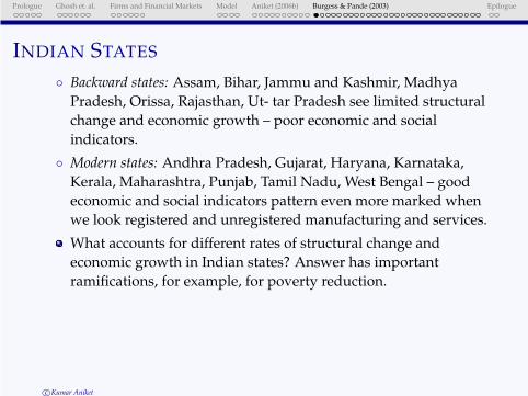
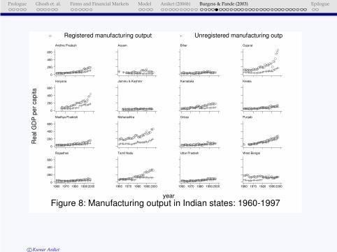
INDIAN STATES
◦ Backward states: Assam, Bihar, Jammu and Kashmir, Madhya
Pradesh, Orissa, Rajasthan, Ut- tar Pradesh see limited structural
change and economic growth – poor economic and social
indicators.
◦ Modern states: Andhra Pradesh, Gujarat, Haryana, Karnataka,
Kerala, Maharashtra, Punjab, Tamil Nadu, West Bengal – good
economic and social indicators pattern even more marked when
we look registered and unregistered manufacturing and services.
What accounts for different rates of structural change and
economic growth in Indian states? Answer has important
ramifications, for example, for poverty reduction.
c©Kumar Aniket
Prologue Ghosh et. al. Firms and Financial Markets Model Aniket (2006b) Burgess & Pande (2003) Epilogue
EVOLUTION OF NON-AGRICULTURAL AND AGRICULTURAL OUTPUT 1961-2000 (AVERAGE ACROSS 16 STATES)
0
500
1000
1500
2000
2500
3000
1961 1964 1967 1970 1973 1976 1979 1982 1985 1988 1991 1994 1997
Non-agricultural output Agricultural output
c©Kumar Aniket
Prologue Ghosh et. al. Firms and Financial Markets Model Aniket (2006b) Burgess & Pande (2003) Epilogue
Re
al G
DP
pe
r ca
pita
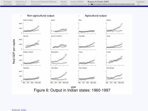
Figure 6: Output in Indian states: 1960-1997year
Non-agricultural output Agricultural output
Andhra Pradesh
0
1000
2000
Assam Bihar Gujarat
Haryana
0
1000
2000
Jammu & Kashmir Karnataka Kerala
Madhya Pradesh
0
1000
2000
Maharashtra Orissa Punjab
Rajasthan
1960 1970 1980 1990 2000
0
1000
2000
Tamil Nadu
1960 1970 1980 1990 2000
Uttar Pradesh
1960 1970 1980 1990 2000
West Bengal
1960 1970 1980 1990 2000
c©Kumar Aniket
Prologue Ghosh et. al. Firms and Financial Markets Model Aniket (2006b) Burgess & Pande (2003) Epilogue
Re
al G
DP
pe
r ca
pita
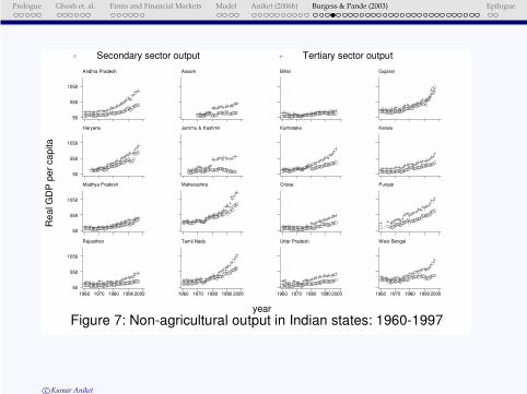
Figure 7: Non-agricultural output in Indian states: 1960-1997year
Secondary sector output Tertiary sector output
Andhra Pradesh
50
550
1050
Assam Bihar Gujarat
Haryana
50
550
1050
Jammu & Kashmir Karnataka Kerala
Madhya Pradesh
50
550
1050
Maharashtra Orissa Punjab
Rajasthan
1960 1970 1980 1990 2000
50
550
1050
Tamil Nadu
1960 1970 1980 1990 2000
Uttar Pradesh
1960 1970 1980 1990 2000
West Bengal
1960 1970 1980 1990 2000
c©Kumar Aniket
Prologue Ghosh et. al. Firms and Financial Markets Model Aniket (2006b) Burgess & Pande (2003) Epilogue
Re
al G
DP
pe
r ca
pita
Figure 8: Manufacturing output in Indian states: 1960-1997year
Registered manufacturing output Unregistered manufacturing outp
Andhra Pradesh
0
200
400
600
Assam Bihar Gujarat
Haryana
0
200
400
600
Jammu & Kashmir Karnataka Kerala
Madhya Pradesh
0
200
400
600
Maharashtra Orissa Punjab
Rajasthan
1960 1970 1980 1990 2000
0
200
400
600
Tamil Nadu
1960 1970 1980 1990 2000
Uttar Pradesh
1960 1970 1980 1990 2000
West Bengal
1960 1970 1980 1990 2000
c©Kumar Aniket
Prologue Ghosh et. al. Firms and Financial Markets Model Aniket (2006b) Burgess & Pande (2003) Epilogue
Pove
rty h
ea
dco
un
t
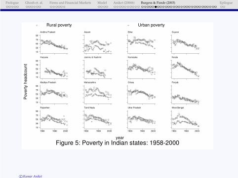
Figure 5: Poverty in Indian states: 1958-2000year
Rural poverty Urban poverty
Andhra Pradesh
10
30
50
70
90
Assam Bihar Gujarat
Haryana
10
30
50
70
90
Jammu & Kashmir Karnataka Kerala
Madhya Pradesh
10
30
50
70
90
Maharashtra Orissa Punjab
Rajasthan
1960 1980 2000
10
30
50
70
90
Tamil Nadu
1960 1980 2000
Uttar Pradesh
1960 1980 2000
West Bengal
1960 1980 2000
c©Kumar Aniket
Prologue Ghosh et. al. Firms and Financial Markets Model Aniket (2006b) Burgess & Pande (2003) Epilogue
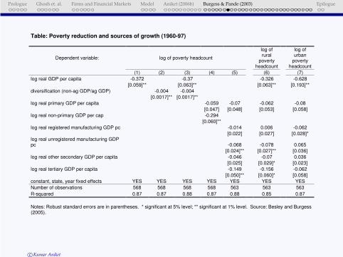
Table: Poverty reduction and sources of growth (1960-97)
Dependent variable: log of poverty headcount
log of rural
povertyheadcount
log of urban
povertyheadcount
(1) (2) (3) (4) (5) (6) (7)
log real GDP per capita -0.372 -0.37 -0.326 -0.628
[0.059]** [0.063]** [0.063]** [0.193]**
diversification (non-ag GDP/ag GDP) -0.004 -0.004
[0.0017]** [0.0017]**
log real primary GDP per capita -0.059 -0.07 -0.062 -0.08
[0.047] [0.048] [0.053] [0.058]
log real non-primary GDP per cap -0.294
[0.060]**
log real registered manufacturing GDP pc -0.014 0.006 -0.062
[0.022] [0.027] [0.028]* log real unregistered manufacturing GDP pc -0.068 -0.078 0.065
[0.024]** [0.027]** [0.036]
log real other secondary GDP per capita -0.046 -0.07 0.036
[0.025] [0.029]* [0.023]
log real tertiary GDP per capita -0.149 -0.156 -0.062
[0.050]** [0.060]* [0.058]
constant, state, year fixed effects YES YES YES YES YES YES YES
Number of observations 568 568 568 568 563 563 563
R-squared 0.87 0.87 0.88 0.87 0.88 0.85 0.87
Notes: Robust standard errors are in parentheses. * significant at 5% level; ** significant at 1% level. Source: Besley and Burgess(2005).
c©Kumar Aniket
Prologue Ghosh et. al. Firms and Financial Markets Model Aniket (2006b) Burgess & Pande (2003) Epilogue
BACKGROUND
◦ Between bank nationalization in 1969 and financial liberalization
in 1990, over 30,000 bank branches opened in rural, un-banked
locations.
◦ Limited evaluation of these type of state-led banking
interventions, which were commonplace in the post war period,
especially in terms of their impact on economic development.
c©Kumar Aniket
Prologue Ghosh et. al. Firms and Financial Markets Model Aniket (2006b) Burgess & Pande (2003) Epilogue
THE LITERATURE
+ The positive view:
à access to bank pre-requisite for structural change and
industrialization (Gerschenkron, 1962)
à access to credit necessary to promote occupational diversification
(Banerjee and Newman, 1993)
– The negative view:
à cheap credit stunts development of private credit markets and
undermines rural development (Adams et al, 1983)
à State ownership and control of banks retards financial
development and hinders economic growth (La Porta, Silanes and
Shleifer, 2002)
c©Kumar Aniket
Prologue Ghosh et. al. Firms and Financial Markets Model Aniket (2006b) Burgess & Pande (2003) Epilogue
INDIA’S BANK NATIONALISATION
India: largest state led rural branch expansion program ever
attempted in a low income country
◦ sharp reduction in regional disparities in population served per
bank branch – more branches were opened in Indian states with
fewer bank branches per capita pre-program (1961)
◦ Hence OLS estimates of the impact of rural branch expansion on
output likely to be biased. (Endogenity)
à Exploit program features to isolate plausibly exogenous (policy
driven) determinants of branch expansion in a state, and use
these as instruments for number of branches opened in rural,
un-banked locations in a state
c©Kumar Aniket
Prologue Ghosh et. al. Firms and Financial Markets Model Aniket (2006b) Burgess & Pande (2003) Epilogue
THE SOCIAL BANKING EXPERIMENT
Branch licensing rule (1977-1990): A bank must open 4 branches in
“un-banked” locations to be eligible to open one in an already banked
location.
1977–90 Negative correlation between state’s initial financial
development and extent of rural branch expansion. The reverse
was true outside this period
1977–90 Output (and more specifically non-agricultural output) fell more
in financially less developed states. The opposite was true
outside this period.
Controlling for a state’s initial financial development and its linear
trend effect on rural branch expansion, state-wise deviations from the
trend in 1977 and 1990 are plausible instruments for the number of
branches opened in un-banked locations in a state
c©Kumar Aniket
Prologue Ghosh et. al. Firms and Financial Markets Model Aniket (2006b) Burgess & Pande (2003) Epilogue
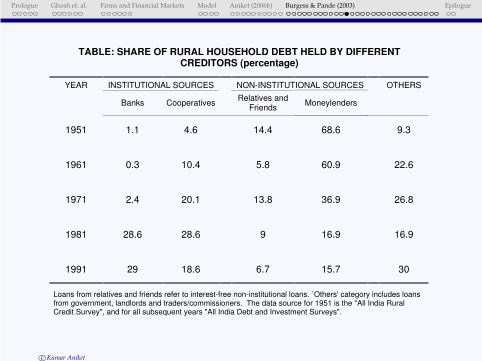
TABLE: SHARE OF RURAL HOUSEHOLD DEBT HELD BY DIFFERENT CREDITORS (percentage)
YEAR INSTITUTIONAL SOURCES NON-INSTITUTIONAL SOURCES OTHERS
Banks CooperativesRelatives and
FriendsMoneylenders
1951 1.1 4.6 14.4 68.6 9.3
1961 0.3 10.4 5.8 60.9 22.6
1971 2.4 20.1 13.8 36.9 26.8
1981 28.6 28.6 9 16.9 16.9
1991 29 18.6 6.7 15.7 30
Loans from relatives and friends refer to interest-free non-institutional loans. `Others' category includes loans from government, landlords and traders/commissioners. The data source for 1951 is the "All India Rural Credit Survey", and for all subsequent years "All India Debt and Investment Surveys".
c©Kumar Aniket
Prologue Ghosh et. al. Firms and Financial Markets Model Aniket (2006b) Burgess & Pande (2003) Epilogue
0
20000
40000
60000
80000
100000
120000
140000
160000
180000
200000
220000
240000
260000
280000
300000
320000
340000
1961 1964 1967 1970 1973 1976 1979 1982 1985 1988 1991 1994 1997 2000
ANDHRA ASSAM BIHAR GUJARAT HARYANA J&K
KARNATAKA KERALA M ADHYAPRADESH M AHARASHTRA ORISSA PUNJAB
RAJASTHAN TAM ILNADU UP WBENGAL
6000
12000
18000
24000
30000
36000
42000
48000
1977 1979 1981 1983 1985 1987 1989 1991 1993 1995 1997 1999
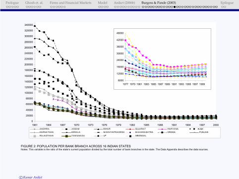
FIGURE 2: POPULATION PER BANK BRANCH ACROSS 16 INDIAN STATES Notes: This variable is the ratio of the state’s current population divided by the total number of bank branches in the state. The Data Appendix describes the data sources.
c©Kumar Aniket
Prologue Ghosh et. al. Firms and Financial Markets Model Aniket (2006b) Burgess & Pande (2003) Epilogue
DATA
Use bank branch level data set which records opening date and
location of every commercial bank branch going back to 1800 to
construct the the following measures:
◦ Initial financial development measure (Bi1961): number of bank
branches per capita in state i in 1961 (i.e. pre-program)
◦ Rural branch expansion measure (BRit): cumulative number of
branches opened per capita in rural un-banked locations in state
i and year t;
c©Kumar Aniket
Prologue Ghosh et. al. Firms and Financial Markets Model Aniket (2006b) Burgess & Pande (2003) Epilogue
IDENTIFICATION STRATEGY
What is the relationship between initial financial development of
a state and subsequent rural branch expansion?
BRit = αi +βt + γt ×Bi1961 +δt ×Xi1961 + εit
= αi +βt +2000
∑t=1961
(Bi1961 ×Dk)γk +2000
∑t=1961
(Xi1961 ×Dk)δk + εit
where Dk = 1 for k = t and Dk = 0 for k 6= t.
Bi1961, the measure of initial financial development, enters the
regression interacted with year dummies, with t denoting the
year-specific coefficients the difference between t+1 and t tells
us how a state’s initial financial development affected rural
branch growth between years t and t+1.
c©Kumar Aniket
Prologue Ghosh et. al. Firms and Financial Markets Model Aniket (2006b) Burgess & Pande (2003) Epilogue
-1.3
-0.8
-0.3
0.2
0.7
1.2
1961 1965 1969 1973 1977 1981 1985 1989 1993 1997
year
Initia
l fin
an
cia
l d
eve
lop
me
nt
X y
ea
r
rural branches in unbanked locations (with controls) rural branches in unbanked locations (implied pattern)
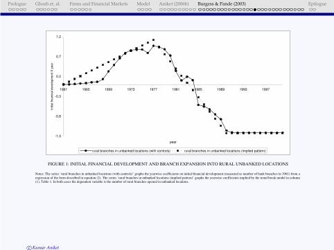
FIGURE 1: INITIAL FINANCIAL DEVELOPMENT AND BRANCH EXPANSION INTO RURAL UNBANKED LOCATIONS
Notes: The series `rural branches in unbanked locations (with controls)’ graphs the yearwise coefficients on initial financial development (measured as number of bank branches in 1961) from a
regression of the form described in equation (2). The series `rural branches in unbanked locations (implied pattern)’ graphs the yearwise coefficients implied by the trend break model in column
(1), Table 1. In both cases the dependent variable is the number of rural branches opened in unbanked locations.
c©Kumar Aniket
Prologue Ghosh et. al. Firms and Financial Markets Model Aniket (2006b) Burgess & Pande (2003) Epilogue
-0.9
-0.6
-0.3
0
0.3
0.6
1961 1965 1969 1973 1977 1981 1985 1989 1993 1997
year
init
ialf
inan
cia
ldevelo
pm
en
tXyear
unbank
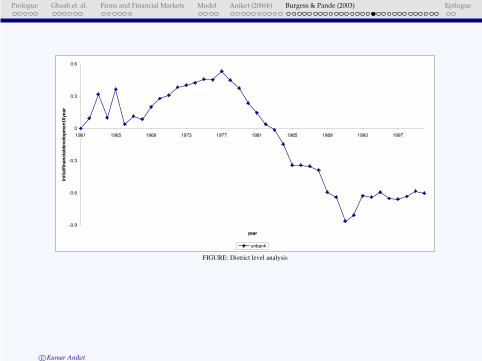
FIGURE: District level analysis
c©Kumar Aniket
Prologue Ghosh et. al. Firms and Financial Markets Model Aniket (2006b) Burgess & Pande (2003) Epilogue
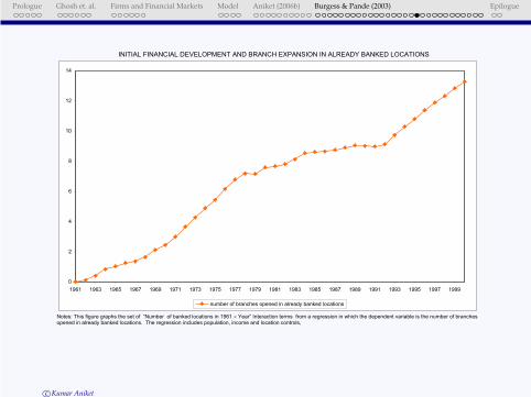
INITIAL FINANCIAL DEVELOPMENT AND BRANCH EXPANSION IN ALREADY BANKED LOCATIONS
0
2
4
6
8
10
12
14
1961 1963 1965 1967 1969 1971 1973 1975 1977 1979 1981 1983 1985 1987 1989 1991 1993 1995 1997 1999
number of branches opened in already banked locations
Notes: This figure graphs the set of “Number of banked locations in 1961 Year” Interaction terms from a regression in which the dependent variable is the number of branches opened in already banked locations. The regression includes population, income and location controls,
c©Kumar Aniket
Prologue Ghosh et. al. Firms and Financial Markets Model Aniket (2006b) Burgess & Pande (2003) Epilogue
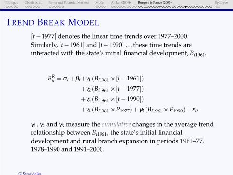
TREND BREAK MODEL
[t−1977] denotes the linear time trends over 1977–2000.
Similarly, [t−1961] and [t−1990] . . . these time trends are
interacted with the state’s initial financial development, Bi1961.
BRit = αi +βt+γ1 (Bi1961 × [t−1961])
+γ2 (Bi1961 × [t−1977])
+γ3 (Bi1961 × [t−1990])
+γ4 (Bi1961 ×P1977)+ γ5 (Bi1961 ×P1990)+ εit
γ1, γ2 and γ3 measure the cumulative changes in the average trend
relationship between Bi1961, the state’s initial financial
development and rural branch expansion in periods 1961–77,
1978–1990 and 1991–2000.
c©Kumar Aniket
Prologue Ghosh et. al. Firms and Financial Markets Model Aniket (2006b) Burgess & Pande (2003) Epilogue
-12
-9
-6
-3
0
3
1969 1973 1977 1981 1985 1989 1993 1997
year
Initia
l fin
an
cia
l d
eve
lop
me
nt X
ye
ar
ruralcredit share
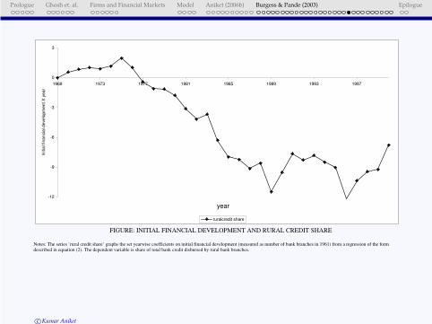
FIGURE: INITIAL FINANCIAL DEVELOPMENT AND RURAL CREDIT SHARE
Notes: The series `rural credit share’ graphs the set yearwise coefficients on initial financial development (measured as number of bank branches in 1961) from a regression of the form
described in equation (2). The dependent variable is share of total bank credit disbursed by rural bank branches.
c©Kumar Aniket
Prologue Ghosh et. al. Firms and Financial Markets Model Aniket (2006b) Burgess & Pande (2003) Epilogue
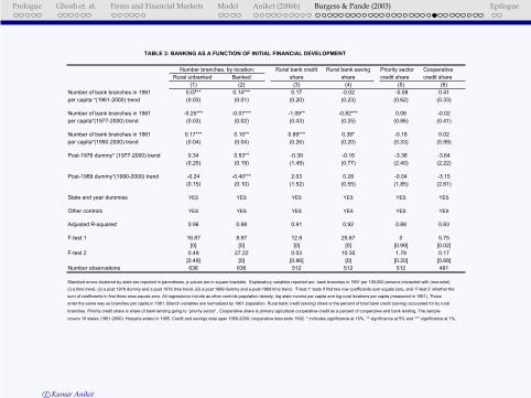
Rural bank credit Rural bank saving Priority sector Cooperative
Rural unbanked Banked share share credit share credit share
(1) (2) (3) (4) (5) (6)
Number of bank branches in 1961 0.07** 0.14*** 0.17 -0.02 -0.08 0.41
per capita *(1961-2000) trend (0.03) (0.01) (0.20) (0.23) (0.62) (0.33)
Number of bank branches in 1961 -0.25*** -0.07*** -1.09** -0.82*** 0.08 -0.02
per capita*(1977-2000) trend (0.03) (0.02) (0.43) (0.25) (0.86) (0.41)
Number of bank branches in 1961 0.17*** 0.10** 0.89*** 0.39* -0.18 0.02
per capita*(1990-2000) trend (0.04) (0.04) (0.26) (0.20) (0.33) (0.99)
Post-1976 dummy* (1977-2000) trend 0.34 0.53** -0.30 -0.16 -3.36 -3.64
(0.25) (0.19) (1.49) (0.77) (2.40) (2.22)
Post-1989 dummy*(1990-2000) trend -0.24 -0.40*** 2.03 0.28 -0.04 -3.15
(0.15) (0.10) (1.52) (0.55) (1.85) (2.61)
State and year dummies YES YES YES YES YES YES
Other controls YES YES YES YES YES YES
Adjusted R-squared 0.96 0.98 0.91 0.92 0.88 0.83
F-test 1 16.87 8.97 12.8 25.67 0 5.75
[0] [0] [0] [0] [0.99] [0.02]
F-test 2 0.49 27.22 0.03 10.35 1.79 0.17
[0.49] [0] [0.86] [0] [0.20] [0.68]
Number observations 636 636 512 512 512 491
TABLE 3: BANKING AS A FUNCTION OF INITIAL FINANCIAL DEVELOPMENT
Number branches, by location:
Standard errors clustered by state are reported in parenthesis, p-values are in square brackets. Explanatory variables reported are bank branches in 1961 per 100,000 persons interacted with (row-wise)
branches. Priority credit share is share of bank lending going to `priority sector' . Cooperative share is primary agicultural cooperative credit as a percent of cooperative and bank lending. The sample
covers 16 states (1961-2000). Haryana enters in 1965. Credit and savings data span 1969-2000; cooperative data ends 1992. * indicates significance at 10%, ** significance at 5% and *** significance at 1%.
(i) a time trend, (ii) a post 1976 dummy and a post 1976 time trend, (iii) a post 1989 dummy and a post-1989 time trend. 'F-test 1' tests if first two row coefficients sum equals zero, and `F-test 2' whether the
sum of coefficients in first three rows equals zero. All regressions include as other controls population density, log state income per capita and log rural locations per capita (measured in 1961). These
enter the same way as branches per capita in 1961. Branch variables are normalized by 1961 population. Rural bank credit (saving) share is the percent of total bank credit (saving) accounted for by rural
c©Kumar Aniket
Prologue Ghosh et. al. Firms and Financial Markets Model Aniket (2006b) Burgess & Pande (2003) Epilogue
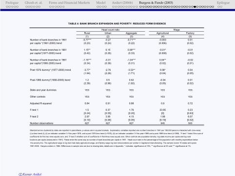
Rural Urban Aggregate Agricultural Factory
(1) (2) (3) (4) (5)
Number of bank branches in 1961 -0.77*** -0.27 -0.71*** -0.003 0.01
per capita *(1961-2000) trend (0.23) (0.24) (0.22) (0.006) (0.02)
Number of bank branches in 1961 1.15** 0.15 0.99*** -0.01* -0.01
per capita*(1977-2000) trend (0.42) (0.26) (0.33) (0.008) (0.02)
Number of bank branches in 1961 -1.15*** -0.31 -1.04*** 0.04** -0.02
per capita*(1990-2000) trend (0.34) (0.38) (0.31) (0.02) (0.01)
Post-1976 dummy* (1977-2000) trend -3.77* -2.76 -3.53** 0.08* 0.04
(1.94) (2.29) (1.71) (0.04) (0.05)
Post-1989 dummy*(1990-2000) trend 1.2 0.5 0.62 -0.04 0.01
(2.39) (0.96) (1.82) (0.05) (0.02)
State and year dummies YES YES YES YES YES
Other controls YES YES YES YES YES
Adjusted R-squared 0.84 0.91 0.88 0.9 0.72
F-test 1 1.5 0.37 1.76 23.95 0.23
[0.24] [0.55] [0.20] [0] [0.63]
F-test 2 2.97 3.95 4.15 1.88 6.07
[0.10] [0.06] [0.05] [0.19] [0.02]
Number observations 627 627 627 545 553
1961-2000. Haryana enters in 1965. Differences in sample size are due to missing data, details are in Appendix. * indicates significance at 10%, ** significance at 5% and *** significance at 1%.
TABLE 4: BANK BRANCH EXPANSION AND POVERTY: REDUCED FORM EVIDENCE
the poverty line. The agricultural wage is log real male daily agricultural wage, and factory wage log real remunerations per worker in registered manufacturing. The sample covers 16 states and spans
Head count ratio
Standard errors clustered by state are reported in parenthesis, p-values are in square brackets. Explanatory variables reported are number branches in 1961 per 100,000 persons interacted with (row-wise)
(i) a time trend (t), (ii) an indicator variable=1 if the year>1976, and a post 1976 time trend (t-1976), (iii) an indicator variable=1 if the year>1989 and a post-1989 time trend (t-1989). 'F-test 1' tests if the sum of
coefficients for first two rows equals zero, and `F-test 2' whether sum of coefficients in first three rows equals zero. Other controls are population density, log state income per capita and log rural
locations per capita (measured in 1961). These enter the same way as number of bank branches per capita in 1961. Head count ratio is the percentage of the population with monthly expenditure below
Wage
c©Kumar Aniket
Prologue Ghosh et. al. Firms and Financial Markets Model Aniket (2006b) Burgess & Pande (2003) Epilogue
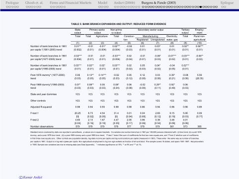
State Non-prima Tertiary Employ-
output ry output output ment
Total Total Agriculture Total Construc- Electricity, Total Rural non-
tion Registered Unregistered water, gas agricultural
(1) (2) (3) (4) (5) (6) (7) (8) (9) (10)
Number of bank branches in 1961 0.01** -0.01 -0.01* 0.02*** -0.02 0.01 0.03* 0.01 0.02** 0.06***
per capita *(1961-2000) trend (0.002) (0.01) (0.004) (0.004) (0.03) (0.01) (0.01) (0.01) (0.01) (0.01)
Number of bank branches in 1961 -0.02*** -0.01 -0.01 -0.03*** 0.02 -0.01 -0.06* -0.07*** -0.03*** -0.06**
per capita*(1977-2000) trend (0.004) (0.01) (0.01) (0.004) (0.04) (0.01) (0.03) (0.02) (0.01) (0.02)
Number of bank branches in 1961 0.03*** 0.02** 0.02* 0.03*** 0.02 0.05 0.04* -0.04 0.02***
per capita*(1990-2000) trend (0.01) (0.01) (0.01) (0.01) (0.02) (0.03) (0.02) (0.05) (0.01)
Post-1976 dummy* (1977-2000) 0.06 0.13** 0.14*** -0.02 0.05 0.12 0.03 0.39* -0.08 5.59
trend (0.03) (0.05) (0.05) (0.03) (0.12) (0.08) (0.06) (0.21) (0.06) (28.35)
Post-1989 dummy*(1990-2000) 0.07* 0.08** 0.05 0.08* 0.06 -0.02 0.29** 0.92* 0.06
trend (0.03) (0.03) (0.03) (0.04) (0.08) (0.09) (0.11) (0.49) (0.03)
State and year dummies YES YES YES YES YES YES YES YES YES YES
Other controls YES YES YES YES YES YES YES YES YES YES
Adjusted R-squared 0.98 0.94 0.93 0.98 0.98 0.86 0.94 0.96 0.98 0.89
F-test 1 20.25 6.73 4.54 31.4 0.01 0.04 2.69 8.15 5.06 0.09
[0] [0.02] [0.05] [0] [0.94] [0.85] [0.12] [0.18] [0.03] [0.77]
F-test 2 4.65 2.13 1.87 4.47 2.05 3.96 0.38 3.48 4.01
[0.04] [0.16] [0.19] [0.05] [0.17] [0.06] [0.54] [0.08] [0.06]
Number observations 579 579 579 579 577 579 579 561 573 365
in 1965. Sample size variations are due to missing data (see Data Appendix). * indicates significance at 10%, ** at 5% and *** at 1%.
Standard errors clustered by state are reported in parenthesis, p-values are in square brackets. Co-variates are number branches in 1961 per 100,000 persons interacted with: (i) time trend, (ii) a post-1976
dummy, and a post-1976 time trend , (iii) a post-1989 dummy and a post-1989 time trend. 'F-test 1' tests if the sum of coefficients for first two rows equals zero, and `F-test 2' whether sum of coefficients
in first three rows equals zero. Other controls are population density, log state income per capita and log rural locations per capita (measured in 1961). These enter the same way as number of branches
TABLE 5: BANK BRANCH EXPANSION AND OUTPUT: REDUCED FORM EVIDENCE
per capita in 1961. Output is in log real rupees per capita. Non agricultural employment is log non-agri workers as fraction of all rural labor. The sample covers 16 states, and spans 1961-1997. Haryana enters
Secondary sector outputPrimary sector
Manufacturing
output
c©Kumar Aniket
Prologue Ghosh et. al. Firms and Financial Markets Model Aniket (2006b) Burgess & Pande (2003) Epilogue
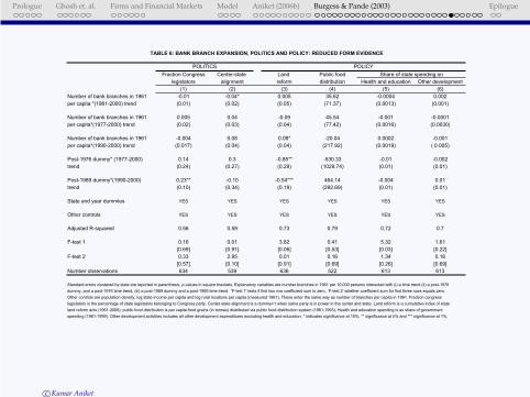
Fraction Congress Center-state Land Public food
legislators alignment reform distribution Health and education Other development
(1) (2) (3) (4) (5) (6)
Number of bank branches in 1961 -0.01 -0.04* 0.005 35.62 -0.0004 0.002
per capita *(1961-2000) trend (0.01) (0.02) (0.05) (71.37) (0.0013) (0.001)
Number of bank branches in 1961 0.005 0.04 -0.09 45.54 -0.001 -0.0001
per capita*(1977-2000) trend (0.02) (0.03) (0.04) (77.42) (0.0016) (0.0030)
Number of bank branches in 1961 -0.004 0.08 0.08* -20.04 0.0002 -0.001
per capita*(1990-2000) trend (0.017) (0.04) (0.04) (217.92) (0.0019) ( 0.005)
Post-1976 dummy* (1977-2000) 0.14 0.3 -0.85** -530.33 -0.01 -0.002
trend (0.24) (0.27) (0.29) (1029.74) (0.01) (0.01)
Post-1989 dummy*(1990-2000) 0.23** -0.10 -0.54*** 464.14 -0.004 0.01
trend (0.10) (0.34) (0.19) (292.69) (0.01) (0.01)
State and year dummies YES YES YES YES YES YES
Other controls YES YES YES YES YES YES
Adjusted R-squared 0.56 0.59 0.73 0.79 0.72 0.7
F-test 1 0.16 0.01 3.82 0.41 5.32 1.61
[0.69] [0.91] [0.06] [0.53] [0.03] [0.22]
F-test 2 0.33 2.95 0.01 0.16 1.34 0.16
[0.57] [0.10] [0.91] [0.69] [0.26] [0.69]
Number observations 634 539 636 522 613 613
land reform acts (1961-2000); public food distribution is per capita food grains (in tonnes) distributed via public food distribution system (1961-1993). Health and education spending is as share of government
spending (1961-1999). Other development activities includes all other development expenditures excluding health and education. * indicates significance at 10%, ** significance at 5% and *** significance at 1%.
dummy, and a post-1976 time trend, (iii) a post-1989 dummy and a post-1989 time trend. 'F-test 1' tests if first two row coefficient sum to zero, `F-test 2' whether coefficient sum for first three rows equals zero.
Other controls are population density, log state income per capita and log rural locations per capita (measured 1961). These enter the same way as number of branches per capita in 1961. Fraction congress
legislators is the percentage of state legislators belonging to Congress party. Center-state alignment is a dummy=1 when same party is in power in the center and state. Land reform is a cumulative index of state
TABLE 6: BANK BRANCH EXPANSION, POLITICS AND POLICY: REDUCED FORM EVIDENCE
Standard errors clustered by state are reported in parenthesis, p-values in square brackets. Explanatory variables are number branches in 1961 per 10,000 persons interacted with (i) a time trend (ii) a post-1976
POLITICS POLICY
Share of state spending on
c©Kumar Aniket
Prologue Ghosh et. al. Firms and Financial Markets Model Aniket (2006b) Burgess & Pande (2003) Epilogue
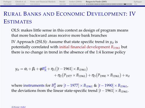
RURAL BANKS AND ECONOMIC DEVELOPMENT: IV
ESTIMATES
OLS: makes little sense in this context as design of program means
that more backward areas receive more bank branches
IV Approach (2SLS): Assume that state specific trend in yit is
potentially correlated with initial financial development Bi1961 but
there is no change in trend in the absence of the 1:4 license policy
yit = αi +βt +φBitR +η1
(
[t−1961]×Bi1961
)
+η2
(
P1977 ×Bi1961
)
+η3
(
P1990 ×Bi1961
)
+uit
where instruments for BRit are [t−1977]×Bi1961 & [t−1990]×Bi1961,
the deviations from the linear state-specific trend [t−1961]×Bi1961.
c©Kumar Aniket
Prologue Ghosh et. al. Firms and Financial Markets Model Aniket (2006b) Burgess & Pande (2003) Epilogue
Urban Aggregate Agricultural Factory
IV IV IV IV IV IV IV IV
1961-89 1977-2000 survey years
(1) (2) (3) (4) (5) (6) (7) (8) (9) (10)
Number branches opened in rural 2.09** 1.15 -4.74** -0.65 -4.10** -4.70** -6.83** -4.20* 0.07* 0.04
unbanked locations per capita (0.79) (1.02) (1.79) (1.06) (1.46) (1.82) (2.80) (2.26) (0.04) (0.08)
IMPLIED ELASTICITY -0.36 -0.32 0.25
Number of bank branches in 1961 -0.43*** -0.47 -0.26* -0.46* -0.43 -0.79* -0.45 -0.006 0.005
per capita * 1961-2000 trend (0.16) (0.26) (0.13) (0.22) (0.26) (0.44) (0.28) (0.003) (0.01)
Post-1976 dummy* (1977-2000) -0.31 -1.42 -2.06 -1.39 -2.13 -1.31 0.04 0.03
trend (1.22) (2.29) (1.65) (2.03) (2.58) (3.32) (0.05) (0.06)
Post-1989 dummy*(1990-2000) 5.37** -1.08 -0.47 -1.55 -0.45 0.78 0.11 -0.05
trend (2.46) (2.33) (1.01) (1.75) (2.90) (2.61) (0.06) (0.04)
State and year dummies YES YES YES YES YES YES YES YES YES YES
Other controls NO YES YES YES YES YES YES YES YES YES
Overidentification test p- 0.99 0.98 0.99 1 0.99 0.99
value
R-squared 0.82 0.85 0.78 0.92 0.81 0.8 0.8 0.77 0.98 0.7
Number observations 627 627 627 627 627 460 375 375 545 553
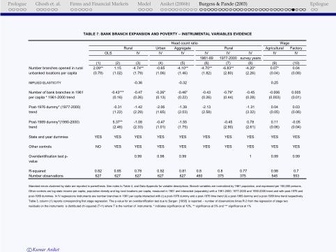
Standard errors clustered by state are reported in parenthesis. See notes to Table 4, and Data Appendix for variable descriptions. Branch variables are normalized by 1961 population, and expressed per 100,000 persons.
Other controls are log state income per capita, population density and log rural locations per capita, measured in 1961 and interacted (separately) with a 1961-2000; 1977-2000 and 1990-2000 trend and with post-1976 and
post-1989 dummies. In IV regressions instruments are number branches in 1961 per capita interacted with (i) a post-1976 dummy and a post-1976 time trend (ii) a post-1989 dummy and a post-1989 time trend respectively.
Table 3, column (1) reports corresponding first stage regression. The p-value for an overidentification test due to Sargan [1958] is reported -- number of observations times R-2 from the regression of stage two
residuals on the instruments is distributed chi-squared (T+1) where T is the number of instruments. * indicates significance at 10%, ** significance at 5% and *** significance at 1%
OLS
TABLE 7: BANK BRANCH EXPANSION AND POVERTY -- INSTRUMENTAL VARIABLES EVIDENCE
Wage
Rural
Head count ratio
Rural
c©Kumar Aniket
Prologue Ghosh et. al. Firms and Financial Markets Model Aniket (2006b) Burgess & Pande (2003) Epilogue
State Non-prima Tertiary Employment
output ry output Electricity, total Non-agri
Total Total Agriculture Total Construction Registered Unregistered water, gas output labor
(1) (2) (3) (4) (5) (6) (7) (8) (9) (10)
Number bank branches in rural 0.08*** 0.04 0.01 0.15*** -0.09 0.05 0.29* 0.30** 0.17*** 0.3
unbanked locations per capita (0.02) (0.03) (0.03) (0.03) (0.19) (0.07) (0.15) (0.13) (0.05) (0.22)
IMPLIED ELASTICITY 0.29 0.55 1.07 1.11 0.62
Number bank branches in 1961 0.004 -0.01* -0.01** 0.01** -0.01 0.01 0.02* -0.02 0.02* 0.06***
per capita * (1961-2000) trend (0.003) (0.00) (0.00) (0.01) (0.02) (0.01) (0.01) (0.02) (0.01) (0.01)
Post-1976 dummy* (1977-2000) 0.004 0.09** 0.12*** -0.1 0.06 0.06 -0.1 0.38* -0.15* -0.03
trend (0.04) (0.04) (0.03) (0.06) (0.17) (0.06) (0.14) (0.19) (0.08) (0.22)
Post-1989 dummy*(1990-2000) 0.15*** 0.16*** 0.13** 0.14*** 0.18 0.16* 0.33** 0.70* 0.08**
trend (0.03) (0.05) (0.04) (0.03) (0.11) (0.08) (0.14) (0.35) (0.03)
State and year dummies YES YES YES YES YES YES YES YES YES YES
Other controls YES YES YES YES YES YES YES YES YES YES
Overidentification test p-value 0.98 0.97 0.97 0.99 0.91 0.97 0.99 0.98 0.99
Adjusted R-squared 0.96 0.93 0.93 0.96 0.98 0.94 0.82 0.7 0.96 0.88
Number observations 579 579 579 579 577 579 579 561 573 365
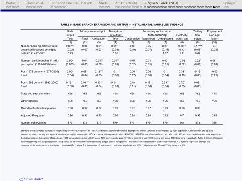
Standard errors clustered by state are reported in parenthesis. See notes to Table 4, and Data Appendix for variable descriptions. Branch variables are normalized by 1961 population. Other controls are log state
income, population density and log rural locations per capita, measured in 1961 and interacted (separately) with 1961-2000; 1977-2000 and 1990-2000 trend and with post-1976 and post-1989 dummies. In IV regressions
the instruments are the number of branches in 1961 per capita interacted with (i) a post-1976 dummy and a post-1976 time trend (ii) a post-1989 dummy and a post-1989 time trend respectively. Table 3, column (1) reports
the corresponding first stage regression. The p-value for an overidentification test due to Sargan [1958] is reported -- the test assumes that number of observations times R-2 from the regression of stage two
residuals on the instruments is distributed chi-squared (T+1) where T is the number of instruments. * indicates significance at 10%, ** significance at 5% and *** significance at 1%
TABLE 8: BANK BRANCH EXPANSION AND OUTPUT -- INSTRUMENTAL VARIABLES EVIDENCE
Primary sector output Secondary sector output
Manufacturing
c©Kumar Aniket
Prologue Ghosh et. al. Firms and Financial Markets Model Aniket (2006b) Burgess & Pande (2003) Epilogue
(1) (2) (3) (4) (5) (6) (7) (8) (9) (10)
Share of bank credit disbursed -1.49** -0.64 0.02* 0.01 0.03**
by rural branches (0.67) (0.45) (0.01) (0.01) (0.02)
Share of bank savings held by -2.27** -1.09 0.02* 0.01 0.03***
rural branches (0.80) (0.69) (0.01) (0.01) (0.01)
Number bank branches in 1961 -0.98* -1.56** -0.69** -1.00** 0.01 0.02** -0.001 -0.001 0.01** 0.02**
per capita * (1961-2000) trend (0.48) (0.59) (0.24) (0.36) (0.01) (0.01) (0.01) (0.01) (0.01) (0.01)
Post-1976 dummy* (1977-2000) -3.00* -1.83 -1.64 -1.13 0.05 0.04 0.11** 0.11** -0.02 -0.03
trend (1.62) (2.29) (1.96) (2.55) (0.05) (0.05) (0.05) (0.05) (0.07) (0.06)
Post-1989 dummy*(1990-2000) 4.56 1.63 2.92 1.65 0.08 0.13*** 0.11 0.14*** 0.05 0.12***
trend (2.64) (2.54) (2.40) (1.27) (0.07) (0.04) (0.07) (0.04) (0.08) (0.04)
State and year dummies YES YES YES YES YES YES YES YES YES YES
Other controls YES YES YES YES YES YES YES YES YES YES
Overidentification test p-value 0.99 0.99 0.99 0.99 0.98 0.95 0.99 0.93 0.99 0.99
Adjusted R-squared 0.72 0.66 0.91 0.89 0.97 0.94 0.98 0.96 0.99 0.97
Number observations 503 503 503 503 463 463 463 463 463 463
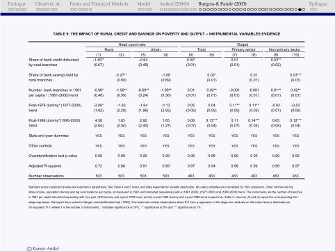
Standard errors clustered by state are reported in parenthesis. See Table 4 and 5 notes, and Data Appendix for variable description. All output variables are normalized by 1961 population. Other controls are log
state income, population density and log rural locations per capita, all measured in 1961 and interacted (separately) with a (1961-2000), (1977-2000) and (1990-2000) trend. The instruments are the number of branches
in 1961 per capita interacted separately with (i) a post-1976 dummy and a post-1976 trend, and (ii) a post-1989 dummy and a post-1989 trend respectively. Table 3, columns (3) and (4) report the corresponding first
stage regression. We report the p-value for Sargan overidentification test [1958]. This assumes number observations times R-2 from a regression of the stage two residuals on the instruments is distributed as
chi-squared (T+1) where T is the number of instruments. * indicates significance at 10%, ** significance at 5% and *** significance at 1%.
Output
Non-primary sector
Head count ratio
TABLE 9: THE IMPACT OF RURAL CREDIT AND SAVINGS ON POVERTY AND OUTPUT -- INSTRUMENTAL VARIABLES EVIDENCE
Rural Urban Total Primary sector
c©Kumar Aniket
Prologue Ghosh et. al. Firms and Financial Markets Model Aniket (2006b) Burgess & Pande (2003) Epilogue
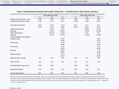
(1) (2) (3) (4) (5) (6)
Number bank branches in rural -4.04** -4.12** -3.77** -0.83 -1.05 -0.81
unbanked locations per capita (1.83) (1.54) (1.54) (1.08) (1.06) (0.91)
Cumulative land reform -1.87** -1.75** -1.87** 0.45 0.41 0.27
(0.79) (0.70) (0.68) (0.28) (0.29) (0.30)
Health and education -10.97 -3.31 23.52 23.74
spending (30.91) (28.40) (14.53) (14.80)
Other Development -40.84*** -37.32** 6.31 5.73
spending (12.39) (13.37) (12.08) (11.89)
Fraction legislators belonging to:
Congress party -13.07 0.22
(8.90) (3.14)
Janata party -11.62 1.62
(6.90) (3.18)
Hindu party 6.15 9.61
(12.91) (8.36)
Hard left -14.81 1.76
(9.07) (3.72)
Regional parties -15.11 -2.34
(12.91) (4.60)
State and year dummies YES YES YES YES YES YES
Other controls YES YES YES YES YES YES
Overidentification test p-value 0.99 0.99 0.98 0.99
Adjusted R-squared 0.78 0.79 0.81 0.92 0.91 0.91
Number observations 627 605 603 627 605 603
Standard errors clustered by state are reported in parenthesis. Table 4 notes, and Data Appendix provide variable description. Branch variables are normalized by 1961 population. Other controls
are log state income, population density and log rural locations per capita, measured in 1961 and interacted (separately) with a (1961-2000), (1977-2000) and (1990-2000) trend. Instruments are number
branches in 1961 per capita interacted with (i) a post-1976 dummy and a post-1976 time trend (ii) a post-1989 dummy and a post-1989 trend respectively. * indicates significance at 10%, ** significance
at 5% and *** significance at 1%.
TABLE 10: BANK BRANCH EXPANSION AND POVERTY REDUCTION -- IV ESTIMATES WITH TIME VARYING CONTROLS
Urban head count ratioRural head count ratio
c©Kumar Aniket
Prologue Ghosh et. al. Firms and Financial Markets Model Aniket (2006b) Burgess & Pande (2003) Epilogue
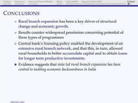
CONCLUSIONS
◦ Rural branch expansion has been a key driver of structural
change and economic growth.
◦ Results counter widespread pessimism concerning potential of
these types of programmes
◦ Central bank’s licensing policy enabled the development of an
extensive rural branch network, and that this, in turn, allowed
rural households to better accumulate capital and to obtain loans
for longer term productive investments.
Evidence suggests that state led rural branch expansion has been
central to tackling economic backwardness in India
c©Kumar Aniket
Prologue Ghosh et. al. Firms and Financial Markets Model Aniket (2006b) Burgess & Pande (2003) Epilogue
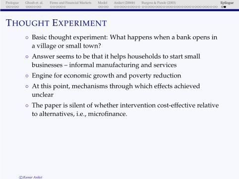
THOUGHT EXPERIMENT
◦ Basic thought experiment: What happens when a bank opens in
a village or small town?
◦ Answer seems to be that it helps households to start small
businesses – informal manufacturing and services
◦ Engine for economic growth and poverty reduction
◦ At this point, mechanisms through which effects achieved
unclear
◦ The paper is silent of whether intervention cost-effective relative
to alternatives, i.e., microfinance.
c©Kumar Aniket