Embed Size (px)
Citation preview

Credit Scoring for Basel II
April 5, 2011
Hans Helbekkmo
Union Bank

2 |
Why Basel II?
Union Bank is opting in to adopt Basel II standards for a variety of reasons:
Former CEO Masa Tanaka on Basel II:
Adopting Basel II “… will allow us to use our own internal models for measuring credit and
operational risk to meet regulatory capital requirements (. . .) under Basel II, banks that take
less risk and incur fewer losses over time are allowed to set aside less regulatory capital.
With lower risks we can expect substantial capital savings compared to banks that have
decided not to opt in under Basel II or those that did opt in but had riskier portfolios.”
Investment in Basel II can lead to:
Better portfolio management with access to more timely and accurate information on
changes affecting risk
Better business decisions with more accurate measurement of economic capital and risk-
adjusted returns
Fewer resources committed to manual data entry, remediation, aggregation, and reporting
(Connections, July 25, 2008)
2 |

3 |
BASEL II Overview – Minimum Capital Charge
• The Basel Accord is structured in three mutually reinforcing sections or “Pillars”:
• Pillar I – calculation of minimum regulatory capital
• Pillar II – supervisory review of overall regulatory capital adequacy as determined by the bank
• Pillar III – disclosure to the market of risk and capital information
• For Advanced-IRB retail portfolios the capital requirement is determined by a complex mathematical
formula that uses Probability of Default (PD), Exposure at Default (EAD) and Loss Given Default
(LGD) as inputs. It is NONLINEAR and based on Asymptotic Single Risk Factor (ASRF) assumption.
This differs from Expected Credit Loss (PD * LGD * EAD).
• The formula will vary according to the following asset types:
• Retail (Mortgages, Qualifying Revolving Exposures (QRE), Other retail)
• Banks determine the following input parameters: PD, LGD and EAD
Minimum Regulatory Capital = EAD * LGD * ƒ (PD, AVC)
Exposure at Default:
an estimate of the amount
the borrower would owe the
Bank at default.
Loss Given Default:
an estimate of percentage of the
EAD that the Bank would expect
to lose in the event of a borrower
default.
Probability of default:
the likelihood of a borrower
defaulting on an obligation
over a 12-month period.
Asset Value Correlation
(AVC): the correlation of
assets among themselves
(non-diversifiable risk). This
varies between assets.
The Basel II formula
specifies the shape of the
unexpected loss curve
(Based on ASRF
assumption)
4 |

4 |
Overview of work leading up to „parallel run‟
2008-2009:
Ensured data sufficiency per Basel II
data requirements
Researched internal portfolio
historical data
Built prototype models
Purchased and installed SAS Credit
Scoring for Banking Solution
software for model building and
implementation
Built production SAS datamart in the
SAS Production Platform
2010-2011:
Built PD, LGD, EAD models and
segmentation calculation for all
portfolios
Completed independent validation of
Mortgage and Home Equity models
Completed formal OCC Review May
2010
Designed Basel II results download
process for the RWA calculation
Scored monthly „live‟ data starting
end of June 2010
Annual model update in early 2011
5 |
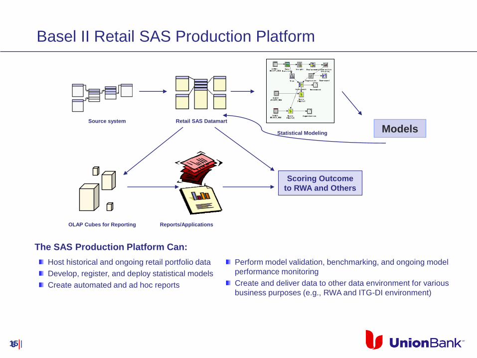
Basel II Retail SAS Production Platform
15 |
Retail SAS Datamart Source system
Models Statistical Modeling
Scoring Outcome
to RWA and Others
Perform model validation, benchmarking, and ongoing model
performance monitoring
Create and deliver data to other data environment for various
business purposes (e.g., RWA and ITG-DI environment)
OLAP Cubes for Reporting Reports/Applications
The SAS Production Platform Can:
Host historical and ongoing retail portfolio data
Develop, register, and deploy statistical models
Create automated and ad hoc reports

6 |
PD, LGD, and EAD Modeling Methodology
The model building process follows several steps:
Data Gathering
• Extracted historical loan origination, account management information to
search insights about the customers
Performance Classification
Probability of Default (PD)
– Charged off or partial charge off or
– Mortgage and Home Equity: 180 days past due, or
– Other Retail Exposures: 120 days past due or charged off
Loss Given Default (LGD)
Exposure at Default (EAD)
Data
Sampling Performance
Classification
Attribute
Analysis
Model
Development Validation and
Refinement
Data
Gathering
7 |
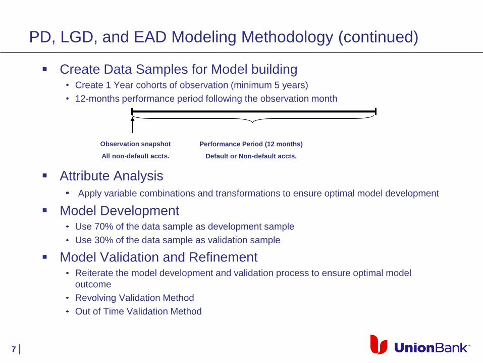
Create Data Samples for Model building
• Create 1 Year cohorts of observation (minimum 5 years)
• 12-months performance period following the observation month
Attribute Analysis
Apply variable combinations and transformations to ensure optimal model development
Model Development Use 70% of the data sample as development sample
Use 30% of the data sample as validation sample
Model Validation and Refinement Reiterate the model development and validation process to ensure optimal model
outcome
Revolving Validation Method
Out of Time Validation Method
Observation snapshot
All non-default accts.
Performance Period (12 months)
Default or Non-default accts.
PD, LGD, and EAD Modeling Methodology (continued)

8 |
Probability of Default Methodology
Current Model
(< 30 DPD Segment)
Loan Level Predicted PD
PD Segmentation Model
(based on segment-level historical default rates)
Origination Model
(Loan Age < 6 Months)
• FICO / Credit Score
• Mortgage type
• Time till int. rt. reset
• Origination LTV
• Co-borrower indicator
Application Characteristics
• Refreshed FICO / Credit Score
• Borrower behavior / payment history
• Time till int. rt. reset
• Utilization rate
•Month on book
• Delinquency status
• Adjusted LTV
Behavior Characteristics
PD estimates by segment
Indeterminate Model
(30 - 179 DPD Segment)
6 |

9 |
Variable transformation – Case/Shiller adjusted LTV
0%
2%
4%
6%
8%
10%
12%
14%
0 10 20 30 40 50 60 70 80 90 100 110 120LTV
Sam
ple
Defa
ult
RA
te
0%
2%
4%
6%
8%
10%
12%
14%
16%
18%
0 - 40 40 - 50 50 - 60 60 - 70 70 - 80 80 - 90 90 - 95 95 - 100 100 - 140LTV
Sam
ple
Defa
ult
Rate
0%
10%
20%
30%
40%
50%
60%
70%
80%
90%
100%
Sam
ple
%
Default Rate
Sample %

10 |
0%
10%
20%
30%
40%
50%
60%
70%
80%
90%
100%
0 10 20 30 40 50 60 70 80 90 100 110 120
LTV
Sam
ple
Defa
ult
RA
te
Variable transformation – Case/Shiller adjusted LTV,
Indeterminates (30-179 days past due)
0%
20%
40%
60%
80%
100%
120%
0 - 30 30 - 40 40 - 50 50 - 60 60 - 70 70 - 80 80 - 90 90 - 140 140 -
LTV
Sa
mp
le D
efa
ult
Ra
te
0%
10%
20%
30%
40%
50%
60%
70%
80%
90%
100%
Sa
mp
le %

11 |
Variable transformation - FICO
0.0%
0.2%
0.4%
0.6%
0.8%
1.0%
1.2%
1.4%
1.6%
1.8%
650 670 690 710 730 750 770 790
Origination FICO
Sa
mp
le d
efa
ult
ra
te
0%
10%
20%
30%
40%
50%
60%
70%
80%
90%
100%
Cu
mu
lati
ve
sa
mp
le %
Bad Rate
Cumulative Dist.

12 |
Variable transformation – Months on Book
0%
5%
10%
15%
20%
25%
< 24 24-30 30-36 36-48 48-54 54-66 > 66
Sam
ple
Defa
ult
Rate
0%
5%
10%
15%
20%
25%
0 12 24 36 48 60 72 84 96
Sam
ple
Defa
ult
Rate

13 |
Probability of Default Result and Model Fit
Portfolio Input VariableRelative
Weight
Refreshed FICO
Score43%
Case Shiller
Adjusted LTV33%
Time Until Interest
Rate Reset13%
Months on Book 12%
Case Shiller
Adjusted CLTV33%
Flex Product
Utilization22%
Refreshed FICO
Score16%
# Times 30-59 DPD 8%
Months on Book 7%
Maximum # Days
Delinquent7%
# Non-sufficient
fund Reversals6%
MT
GH
EMortgage and Home Equity PD models were estimated based on Weights of Evidence transformation of the risk
drivers. The selected risk drivers and the corresponding weights in the production models are shown on the left.
The model fit assessment by ROC curve and index are shown on the right:
Current Model Mortgage
Home Equity
ROC Index 0.91
ROC Index 0.96
8 |

14 |
Predictive power backtesting
Split between training sample (70%)
and validation sample (30%)
ROC curve (Validation)
Additional Out-of-Sample Validation
Measure Train ValidateROC 0.92 0.91
KS 0.73 0.71
Input Variable AB AC BC
Intercept -2.184 -2.266 -2.265
Case Shiller Adjusted LTV -0.564 -0.590 -0.555
Refreshed FICO Score -0.576 -0.606 -0.637
Month on Books -0.334 -0.483 -0.277
Time Until Interest Rate Reset -0.426 -0.288 -0.481
Measure AB AC BC
ROC 0.93 0.92 0.91KS 0.74 0.73 0.71
Input VariableBuild on 2002-2008
Validate on 2009
Build on 2009
Validate on 2002-2008
Intercept -2.249 -2.042
Case Shiller Adjusted LTV -0.611 -0.435
Refreshed FICO Score -0.575 -0.655
Month on Books -0.293 -0.577
Time Until Interest Rate Reset -0.490 -0.227
MeasureBuild on 2002-2008
Validate on 2009
Build on 2009
Validate on 2002-2008
ROC 0.85 0.89
KS 0.60 0.67
0
0.1
0.2
0.3
0.4
0.5
0.6
0.7
0.8
0.9
1
0 0.1 0.2 0.3 0.4 0.5 0.6 0.7 0.8 0.9 1
Additional Out-of-Time Validation

15 |
Predictive accuracy back-testing
9 |
Besides fit assessment of the PD models, back-testing is another important and necessary assessment of the
models‟ predictive power and accuracy. The basic idea of back-testing is to examine how “closely” the prediction
of PD tracks the actual historical default rate across different dimensions.
y = 1.0049x + 0.0002R² = 0.9874
0%
10%
20%
30%
40%
50%
60%
70%
80%
90%
100%
0% 20% 40% 60% 80% 100%
Actu
al P
D
Predicted PD
Mortgage PD Predicted vs. Actual
Pred. vs. Act.
Cum. Dist.
Linear (Pred. vs. Act.)
y = 0.9827x + 0.0011R² = 0.9909
0%
10%
20%
30%
40%
50%
60%
70%
80%
90%
100%
0% 20% 40% 60% 80% 100%
Actu
al P
D
Predicted PD
HE PD Predicted vs. Actual
Pred. vs. Act.
Cum. Dist.
Linear (Pred. vs. Act.)
0.0%
0.2%
0.4%
0.6%
0.8%
1.0%
1.2%
1.4%
Jan
-02
Jul-
02
Jan
-03
Jul-
03
Jan
-04
Jul-
04
Jan
-05
Jul-
05
Jan
-06
Jul-
06
Jan
-07
Jul-
07
Jan
-08
Jul-
08
Jan
-09
Jul-
09
Mortgage PD Back-testing across time
Actual D.R.
Pred. D.R.
0.0%
0.2%
0.4%
0.6%
0.8%
1.0%
1.2%
1.4%
Jan
-03
Jul-
03
Jan
-04
Jul-
04
Jan
-05
Jul-
05
Jan
-06
Jul-
06
Jan
-07
Jul-
07
Jan
-08
Jul-
08
Jan
-09
Jul-
09
HE PD Back-testing across Time
Actual D.R.
Pred. D.R.

16 |
SAS Enterprise-Miner Example
SAS E-Miner
Different nodes in the E-Miner
allows you to:
Explore the data
Perform statistical analysis
Treat missing values
Transform variables
Group variables with similar
characteristics
Build multiple statistical
models
Compare model outcome
using validation data
Select the best model
Package the final model for
deployment
16

17 |
Loss Given Default Methodology
• Loss Give Default (LGD): notion of “economic loss” which should capture all material credit-related losses on
the exposure (including accrued but unpaid interest or fees, losses on the sale of repossessed collateral, direct
workout costs and an appropriate allocation of indirect workout costs), on a net present value basis as of the
default date using a discount rate appropriate to the risk of the exposure
where
and the net loss is calculated based on the following components:
• LGD Models for both Mortgage and Home Equity were developed on all default accounts January 2002 – January
2009
𝑳𝑮𝑫 =𝑳𝒐𝒔𝒔 (𝒊𝒏𝒄𝒍𝒖𝒅𝒊𝒏𝒈 𝒇𝒆𝒆𝒔 𝒂𝒏𝒅 𝒊𝒏𝒕𝒆𝒓𝒆𝒔𝒕) + 𝑾𝒐𝒓𝒌𝒐𝒖𝒕 𝑪𝒐𝒔𝒕𝒔
𝑬𝑨𝑫
𝑬𝑨𝑫 = 𝑩𝒂𝒍𝒂𝒏𝒄𝒆 𝑼𝒏𝒑𝒂𝒊𝒅+ 𝑰𝒏𝒕𝒆𝒓𝒆𝒔𝒕 𝑼𝒏𝒑𝒂𝒊𝒅+ 𝑭𝒆𝒆𝒔 𝑼𝒏𝒑𝒂𝒊𝒅+ 𝑳𝒂𝒕𝒆𝑪𝒉𝒂𝒓𝒈𝒆 𝑼𝒏𝒑𝒂𝒊𝒅
10 |
Loss / Recovery Component Unresolved Properties Resolved Properties
Balance, Fees and Interest X X
Charge-off Principal X
REO Costs X X
REO Principal Writedowns X
REO Recoveries X X
REO Property Sales X
Short Sales X
Paid in Full Events X
Writedown Report Expected Loss X

18 |
Sample LGD data
Transaction level cashflow data for REO portfolio
Type Date Name Memo Debit Credit
Bill 1/4/2000 Book In Blance $95,727
Bill 3/17/2000 Rekey and Secure $129
Bill 3/20/2000 99/2000 2nd Installment $386
Bill 4/7/2000 Utilities $8
Bill 4/7/2000 Board W indows/Fence $625
Bill 4/7/2000 Pest Report $105
Bill 4/10/2000 Property Value W ritedown $21,327
Deposit 4/10/2000 W ritedown $21,327
Bill 4/14/2000 Eviction Proceedings $1,887
Bill 4/14/2000 Trashout/Clean $600
Bill 4/14/2000 Yard Maintenance $150
Bill 4/14/2000 Alarms and Straps $155
Bill 4/14/2000 W ash and Belach Mold from W alls $225
Bill 4/14/2000 Remove Carpet and Haul to Dump $250
Bill 4/19/2000
trashout int. & ext. cleanup of property,
remove carpet/hual, strap w/h, install
smoke dect.
$1,380
Bill 4/24/2000 electric bill $4
Bill 5/19/2000 W ater $166
Bill 5/19/2000 Yard Maintenance $100
Bill 6/15/2000 $4
Bill 6/20/2000 Utilities $79
Deposit 6/27/2000 Sale Price $75000 $74,400
Deposit 6/27/2000 Sale Price $75,000 $615
Bill 7/24/2000 $100
Bill 7/24/2000 $100
Bill 7/24/2000 $7
Bill 3/1/2001 1999 SUPPLEMENTAL ASSESSMENT $127
RC # 72200
Residential:2000-001
10209 Las Tunas
Rancho Cordova

19 |
Loss Given Default Result and Back-testing
LGD was estimated by a hybrid approach: calculate segment level account weighted LGD based on estimated loan
level. The selected risk drivers and the corresponding weights in the production models are shown on the left. The
model back-testing across time results are shown on the right:
Portfolio Input VariableRelative
Weight
Months on Book 32%
Loan Balance 29%
Case Shiller
Adjusted LTV26%
Fix Rate Indicator 13%
Case Shiller
Adjusted CLTV50%
First Lien Indicator 29%
Months on Book 26%
Current
Commitment13%
MTG
HE
Loan - level Model
11 |
0%
20%
40%
60%
80%
100%
120%
10% 20% 30% 40% 50% 60% 70% 80% 90% 100%
Home Equity LGD Back-testing - By Decile
Actual LGD Predicted LGD
0%
10%
20%
30%
40%
50%
60%
70%
80%
10% 20% 30% 40% 50% 60% 70% 80% 90% 100%
Mortgage LGD Back-testing - By Decile
Actual LGD Predicted LGD

20 |
Mortgage segmentation
Segment ID PD Segment DPD LGD Segment # Accts Total Balance Avg PD Avg LGDAssigned
PD
Assigned
LGDBasel Captial
1 < .04% < 30 DPD < 19.5% 1,985 $748,099,813 0.0% 7.8% 0.03% $1,368,457.05
2 .04% - .16% < 30 DPD < 19.5% 3,102 $2,699,323,424 0.1% 7.0% 0.1% $10,976,045.03
3 .16% - .75% < 30 DPD < 19.5% 3,915 $4,504,934,437 0.4% 6.8% 0.3% $35,092,625.04
4 .75% - 2.23% < 30 DPD < 19.5% 1,619 $1,988,543,016 1.2% 7.3% 1.4% $38,499,237.03
5 2.23% - 4.58% < 30 DPD < 19.5% 378 $476,765,401 3.0% 6.8% 3.4% $14,841,043.34
6 > 4.58% < 30 DPD < 19.5% 145 $207,080,397 10.8% 7.0% 12.7% $11,087,610.66
7 < 5.1% 30-179 DPD < 19.5% 24 $3,372,474 2.5% 4.4% 2.1% $83,366.61
8 5.1% - 21.1% 30-179 DPD < 19.5% 27 $12,544,427 9.9% 6.8% 7.2% $551,289.41
9 21.1% - 72.5% 30-179 DPD < 19.5% 68 $75,240,491 43.4% 6.7% 43.1% $4,241,615.96
10 >72.5% 30-179 DPD < 19.5% 34 $47,053,563 89.5% 5.9% 86.5% $793,517.43
11 < .04% < 30 DPD 19.5% - 33.2% 2,120 $276,074,371 0.0% 26.6% 0.03% $956,169.91
12 .04% - .16% < 30 DPD 19.5% - 33.2% 2,224 $625,300,707 0.1% 26.2% 0.1% $5,231,496.83
13 .16% - .75% < 30 DPD 19.5% - 33.2% 2,562 $1,332,502,426 0.4% 25.8% 0.3% $21,357,060.55
14 .75% - 2.23% < 30 DPD 19.5% - 33.2% 1,487 $883,019,530 1.3% 26.3% 1.4% $35,174,953.45
15 2.23% - 4.58% < 30 DPD 19.5% - 33.2% 339 $211,986,704 3.1% 26.8% 3.4% $13,577,331.25
16 > 4.58% < 30 DPD 19.5% - 33.2% 150 $89,656,692 9.7% 26.5% 12.7% $9,877,061.97
17 < 5.1% 30-179 DPD 19.5% - 33.2% 6 $1,197,872 2.1% 26.3% 2.1% $60,925.64
18 5.1% - 21.1% 30-179 DPD 19.5% - 33.2% 20 $4,796,369 12.8% 26.8% 7.2% $433,698.13
19 21.1% - 72.5% 30-179 DPD 19.5% - 33.2% 77 $40,147,065 46.8% 26.9% 43.1% $4,656,714.57
20 >72.5% 30-179 DPD 19.5% - 33.2% 41 $22,028,809 88.3% 26.1% 86.5% $764,365.47
21 < .04% < 30 DPD > 33.2% 788 $97,511,336 0.0% 37.1% 0.03% $480,110.94
22 .04% - .16% < 30 DPD > 33.2% 2,589 $382,155,766 0.1% 39.6% 0.1% $4,545,220.77
23 .16% - .75% < 30 DPD > 33.2% 3,040 $714,125,518 0.4% 41.3% 0.3% $16,271,423.29
24 .75% - 2.23% < 30 DPD > 33.2% 2,197 $717,952,972 1.3% 41.7% 1.4% $40,657,132.05
25 2.23% - 4.58% < 30 DPD > 33.2% 678 $237,304,610 3.2% 42.7% 3.4% $21,606,752.02
26 > 4.58% < 30 DPD > 33.2% 368 $112,322,038 10.4% 43.1% 12.7% $17,590,879.89
27 < 5.1% 30-179 DPD > 33.2% 2 $99,747 2.5% 35.3% 2.1% $7,212.16
28 5.1% - 21.1% 30-179 DPD > 33.2% 10 $1,850,528 12.7% 34.4% 7.2% $237,874.67
29 21.1% - 72.5% 30-179 DPD > 33.2% 117 $29,575,192 47.8% 41.8% 43.1% $4,876,754.66
30 >72.5% 30-179 DPD > 33.2% 83 $27,015,982 90.2% 42.3% 86.5% $1,332,626.13
31 Default Default Default 250 $139,090,049 100.0% 8.0% 100.0% 8% $11,127,203.91
$328,357,775.84
13.6%
27.9%
39.7%

21 |
Credit Analytics Applications
Credit Analytics not only can be utilized to estimate minimum regulatory capital and economic capital the bank
uses to cushion unexpected losses, but it can also be leveraged by Credit Portfolio Risk Management to
optimize risk-reward profile of new originations as well as actively and effectively manage the bank‟s risk
position.
12 |
Credit Analytics Applications “Organic Growth”
(New Originations)
Risk-based Decision
(Existing Portfolios)
Optimize risk-reward profile by effectively allocating capital
across geography, product type, line of business, etc.
Leverage the data collected and model outputs to analyze risk
sensitivity to the business cycle and adjust the Bank‟s growth
strategy as needed
Understand changes in industry behavior and market direction
to promptly identify negative trends, allowing for early risk
mitigation actions, hedging and dynamic portfolio optimization
Leverage risk-adjusted return metric to create customized
pricing strategies.
Understand the risk-reward profile of asset classes to drive
enterprise-level concentration management, asset allocation
strategies and stress testing to mitigate against “one-time large-
loss” events that require costly capital raising
Leverage the data collected to develop early warning signals
that prompt risk mitigation actions


![Validation of Internal Rating and Scoring Models ... of Internal Rating and Scoring ... [Basel II, §500] ... Basel I Advanced IRB Credit Risk AMA Operational Risk](https://img.pdfslide.net/doc/110x75/5ab075ad7f8b9a6b468b4b66/validation-of-internal-rating-and-scoring-models-of-internal-rating-and-scoring.jpg)