Mossavar-Rahmani Center for Business & Government

Weil Hall | Harvard Kennedy School | www.hks.harvard.edu/mrcbg

M-RCBG Associate Working Paper Series | No. 8

The views expressed in the M-RCBG Fellows and Graduate Student Research Paper Series are those of

the author(s) and do not necessarily reflect those of the Mossavar-Rahmani Center for Business &

Government or of Harvard University. The papers in this series have not undergone formal review and

approval; they are presented to elicit feedback and to encourage debate on important public policy

challenges. Copyright belongs to the author(s). Papers may be downloaded for personal use only.

Crime, Weather, and Climate Change

Matthew Ranson Harvard Kennedy School

May 2012

Crime, Weather, and Climate Change

Matthew Ranson∗

May 31, 2012

Abstract

This paper estimates the impact of climate change on the prevalence of criminal activityin the United States. The analysis is based on a panel of monthly crime, temperature, andprecipitation data for 2,972 U.S. counties over the 50-year period from 1960 to 2009. I identifythe effect of weather on monthly crime by using a semi-parametric bin estimator and control-ling for county-by-month and county-by-year fixed effects. The results show that temperaturehas a strong positive effect on criminal behavior, with little evidence of lagged impacts. Underthe IPCC’s A1B climate scenario, the United States will experience an additional 35,000 mur-ders, 216,000 cases of rape, 1.6 million aggraved assaults, 2.4 million simple assaults, 409,000robberies, 3.1 million burglaries, 3.8 million cases of larceny, and 1.4 million cases of vehicletheft, compared to the total number of offenses that would have occurred between the years2010 and 2099 in the absence of climate change. The present discounted value of the socialcosts of these climate-related crimes is between 20 and 68 billion dollars.

∗PhD Candidate in Public Policy, Harvard University, 79 John F. Kennedy Street, Cambridge, MA, 02138 (email:ranson@post.harvard.edu). I am grateful for helpful comments received from Erich Muehlegger, Robert Stavins,Martin Weitzman, Richard Zeckhauser, and seminar participants at Harvard University. Any errors are my own.

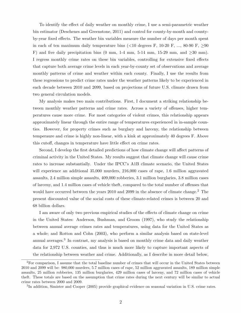
1 Introduction

The short-term effects of weather on crime are well documented. Previous work has shown that

presumably-random variation in daily and weekly temperatures affects the incidence of both

violent and non-violent offenses, with higher temperatures leading to higher levels of criminal

activity (Brunsdon et al, 2009; Bushman, Wang, and Anderson, 2005; Cohn, 1990). However,

despite the strength of this relationship, there is little evidence on how weather affects patterns

of criminal behavior over longer time scales. In particular, there is great uncertainty about

how climate change is likely to affect the incidence of crime.

The Intergovernmental Panel on Climate Change predicts that global temperatures are

likely to rise by about 5 degrees Fahrenheit (2.8 degrees Celsius) by the year 2099, compared

to baseline temperatures during the period from 1980 to 1999 (IPCC, 2007). Studies of the

short-term relationship between crime and weather suggest that such a change in temperatures

could have dramatic effects on crime patterns. However, given that crime rates exhibit negative

serial correlation over the scale of days to weeks (Jacob, Lefgren, and Moretti, 2007), the long-

term impacts of climate change on crime may be considerably smaller than the short-term

impacts. The only two previous studies of the effects of climate change on crime have used

highly aggregate data and found mixed results (Anderson, Bushman, and Groom, 1997; Rotton

and Cohn, 2003). To address this gap in the literature, in this paper I use an unusually long and

rich panel dataset to estimate the historical relationship between weather and crime. I then

use this historical relationship to predict how climate change will impact the future prevalence

of criminal activity in the United States, based on existing simulations of future weather under

the IPCC’s A1B scenario.1

To support my analysis, I have constructed a panel dataset that includes monthly crime

and weather data for 2,972 U.S. counties for the period from 1960 to 2009. My data on

criminal activity is drawn from the U.S. Federal Bureau of Investigation’s Uniform Crime

Reporting (UCR) data. These data, which are based on monthly reports from 17,000 U.S.

law enforcement agencies, tabulate offenses in nine major categories: murder, manslaughter,

rape, aggravated assault, simple assault, robbery, burglary, larceny, and vehicle theft. I merge

this data on crime rates with historical weather data from the U.S. National Climatic Data

Center’s Global Historical Climatology Network Daily (GHCN-Daily) dataset. The GHCN-

Daily weather data include temperature and precipitation records from 75,000 weather stations

worldwide that have been subjected to a set of quality assurance checks. After combining

these two data sources, I generate a dataset with 1.46 million unique county-by-year-by-month

observations.

1All climate projections cited in this paper are based on the IPCC’s A1B scenario. This scenario represents afuture world with high rates of economic growth and substantial convergence between developing and developedeconomies, where rapid technological change is based on a balance of fossil-fuel intensive and non-fossil sources ofenergy (IPCC, 2000). A1B is a “middle-of-the-road” scenario that tends to produce emissions and climate resultsthat are intermediate between high emissions scenarios such as A1FI and low emissions scenarios such as B1.

1

To identify the effect of daily weather on monthly crime, I use a semi-parametric weather

bin estimator (Deschenes and Greenstone, 2011) and control for county-by-month and county-

by-year fixed effects. The weather bin variables measure the number of days per month spent

in each of ten maximum daily temperature bins (<10 degrees F, 10-20 F, ..., 80-90 F, ≥90

F) and five daily precipitation bins (0 mm, 1-4 mm, 5-14 mm, 15-29 mm, and ≥30 mm).

I regress monthly crime rates on these bin variables, controlling for extensive fixed effects

that capture both average crime levels in each year-by-county set of observations and average

monthly patterns of crime and weather within each county. Finally, I use the results from

these regressions to predict crime rates under the weather patterns likely to be experienced in

each decade between 2010 and 2099, based on projections of future U.S. climate drawn from

two general circulation models.

My analysis makes two main contributions. First, I document a striking relationship be-

tween monthly weather patterns and crime rates. Across a variety of offenses, higher tem-

peratures cause more crime. For most categories of violent crimes, this relationship appears

approximately linear through the entire range of temperatures experienced in in-sample coun-

ties. However, for property crimes such as burglary and larceny, the relationship between

temperaure and crime is highly non-linear, with a kink at approximately 40 degrees F. Above

this cutoff, changes in temperature have little effect on crime rates.

Second, I develop the first detailed predictions of how climate change will affect patterns of

criminal activity in the United States. My results suggest that climate change will cause crime

rates to increase substantially. Under the IPCC’s A1B climate scenario, the United States

will experience an additional 35,000 murders, 216,000 cases of rape, 1.6 million aggravated

assaults, 2.4 million simple assaults, 409,000 robberies, 3.1 million burglaries, 3.8 million cases

of larceny, and 1.4 million cases of vehicle theft, compared to the total number of offenses that

would have occurred between the years 2010 and 2099 in the absence of climate change.2 The

present discounted value of the social costs of these climate-related crimes is between 20 and

68 billion dollars.

I am aware of only two previous empirical studies of the effects of climate change on crime

in the United States: Anderson, Bushman, and Groom (1997), who study the relationship

between annual average crimes rates and temperatures, using data for the United States as

a whole; and Rotton and Cohn (2003), who perform a similar analysis based on state-level

annual averages.3 In contrast, my analysis is based on monthly crime data and daily weather

data for 2,972 U.S. counties, and thus is much more likely to capture important aspects of

the relationship between weather and crime. Additionally, as I describe in more detail below,

2For comparison, I assume that the total baseline number of crimes that will occur in the United States between2010 and 2099 will be: 980,000 murders, 5.7 million cases of rape, 52 million aggravated assaults, 189 million simpleassaults, 25 million robberies, 135 million burglaries, 429 million cases of larceny, and 72 million cases of vehicletheft. These totals are based on the assumption that crime rates during the next century will be similar to actualcrime rates between 2000 and 2009.

3In addition, Simister and Cooper (2005) provide graphical evidence on seasonal variation in U.S. crime rates.

2

reporting inconsistencies in the FBI’s crime data add considerable measurement error to in-

terannual comparisons of crime rates. Thus, by focusing on month-to-month changes in crime

rates within a particular county and year, my analysis solves measurement error issues that

have plagued previous work.

The remainder of this paper is organized as follows. Section 2 provides background on the

relationship between weather and crime. Section 3 describes the primary data sources, and

Section 4 discusses my empirical methodology. Section 5 presents my main findings on the

relationship between climate change and crime. Section 6 discusses the results and Section 7

concludes.

2 Background on Weather and Crime

Researchers have proposed several hypotheses that explain why weather might affect crime

(Cohn, 1990; Agnew, 2012). The first—that weather is a variable in the production function for

crime—draws on Gary Becker’s canonical model of crime, in which individuals make decisions

about whether to commit criminal acts based on rational consideration of the costs and benefits

(Becker, 1968). In this model, weather conditions are an input that affects both the probability

of successfully completing a crime and the probability of escaping undetected afterward (Jacob,

Lefgren, and Moretti, 2007). For example, pleasant evening weather may increase the number

of opportunities for mugging, and dark, rainy nights may increase the probability of successfully

burglarizing a house without being detected.

A second explanation draws on a social interaction theory of crime. Glaeser, Sacerdote,

and Scheinkman (1996) propose that the frequency of criminal acts is driven in large part by

social interactions that occur during day-to-day life. Applied to weather, such a hypothesis

implies that weather conditions that foster social interactions are likely to increase crime rates

(Rotton and Cohn, 2003). For example, mild weather that encourages people to go shopping

would also have the effect of increasing the frequency of property crimes such as larceny.

A third possible explanation draws on theories in which external conditions directly affect

human judgment in ways that cause heightened aggression and loss of control (Baumeister

and Heatherton, 1996; Card and Dahl, 2011). Experimental evidence strongly suggests that

ambient temperatures affect aggression (Anderson, 1989). For example, Baron and Bell (1976)

assigned male subjects to receive a positive or negative evaluation from a confederate, and then

gave them the opportunity to retaliate with an elecric shock. They found that retaliation was

highest when the experiment took place in a room with a high ambient temperature (92-95

degrees F), and that retaliation was still heightened even at more moderate temperatures (82-

85 degrees F). Such studies imply that weather may directly influence people’s psychological

propensity to commit violent criminal acts.

Although using empirical data to distinguish between these hypotheses is difficult, there

is considerable evidence that weather does affect criminal behavior (Cohn, 1990). Previous

3

research on this topic has typically taken one of two empirical approaches. First, some studies

have focused on measuring the short-term relationship between weather and crime, using

hourly, daily, or weekly microdata (Bushman, Wang, and Anderson, 2005; Cohn and Rotton,

2000). For example, Brunsdon et al (2009) measure the impact of weather on disorderly

conduct using hourly data on police calls in an urban area of the United Kingdom. They

find that disorderly conduct increases with temperature and humidity but is unaffected by

precipitation. However, interpreting these types of studies in the context of climate change

is complicated by negative serial correlation in crime. In a large study using weekly data on

crime and temperatures in 116 U.S. jurisdictions for the period 1996 to 2001, Jacob, Lefgren,

and Moretti (2007) find that although rates of violent crime and property crime are elevated

during weeks with hot weather, the effect is offset somewhat by lower than usual crime rates in

the following weeks. This result suggests that understanding the cumulative impacts of climate

change on crime may require working with data at a more aggregate time scale (e.g., months).

Simister and Cooper (2005) conduct such an analysis for Los Angeles, using monthly assault

and weather data from 1988 to 2002. Based on regressions that include linear and quadratic

effects, they find evidence of a strong linear relationship between assault and temperature.4

The second main empirical approach in the literature is to use yearly data to measure how

weather affects crime at the national or state levels. For example, authors have examined

the time series relationship between annual average crimes rates and average temperatures,

for the United States as a whole (Anderson, Bushman, and Groom, 1997) and for a panel of

states (Rotton and Cohn, 2003). These studies have found mixed results, possibily due to

the a lack of geographic and spatial resolution in the crime and weather data. Another issue

with this work is that U.S. aggregate crime statistics suffer from known quality issues, with

different data sources implying considerably different trends in crime rates in the 1970s and

1980s (Levitt, 2004). As a result, analyses based on such geographically-aggregate annual data

may face econometric issues with measurement error.

3 Data

3.1 Data Sources

The analysis for this paper is based on an unusually long and rich panel dataset of monthly

crime rates and weather for 2,972 counties in the 49 continental states (including the District

of Columbia). The dataset covers the 50-year period from 1960 to 2009, and contains 1.46

million unique county-by-year-by-month observations. It is based on two primary sources:

Uniform Crime Reporting data from the U.S. Federal Bureau of Investigation (FBI, 2011a),

4Simister (2002) and Simister and Van de Vliert (2005) find evidence of an approximately linear relationshipbetween temperature and murder in a similar analysis using national-level monthly data on weather and murder forPakistan.

4

and Global Historical Climatology Network Daily weather data from the National Climatic

Data Center (NCDC Climate Services Branch, 2011).

The FBI’s Uniform Crime Reporting (UCR) data are the longest continuously-collected

historical record of criminal activity in the United States. These data are based on monthly

reports from approximately 17,000 local, county, city, university, state, and tribal law enforce-

ment agencies. Although participation is voluntary and has increased over time, in 2010 the

UCR data covered law enforcement agencies representing 97.4 percent of the U.S. population

(FBI, 2011b). The data submitted by each agency each month include the number of reported

offenses of murder, manslaughter, rape, aggravated assault, simple assault, robbery, burglary,

larceny, and vehicle theft. Table 1 summarizes the definitions of each offense. In cases when

a crime falls into more than one category, the FBI uses a “heirarchy rule” to assign the crime

to the most serious offense category (FBI, 2004).

A central challenge in using the agency-level UCR data to construct monthly county-level

crime rate time series is that the number of reported crimes in the data increases dramatically

through the 1960s and 1970s, due both to changes in the number of agencies reporting and to

more comprehensive reporting by individual agencies. Because of these limitations, developing

a county-level time series that is consistent across years would involve considerable researcher

judgment about non-reporting bias (and would most likely require excluding a large number

of observations from the analysis). Although previous research on criminal behavior has made

use of such annual UCR data (e.g., Levitt, 1996), in this paper I take a different approach in

which I construct a time series that is consistent only across months within each county-by-

year group of observations. To build this time series, I first drop any agency-by-year records

in which an agency reported less than twelve months of data for that year.5 I then sum

the total number of reported crimes by all remaining agencies in each county, by category of

crime, to generate a county total for each month and year. Finally, using county population

data from the U.S. Census (U.S. Census Bureau, 1978, 2004, 2011), I calculate the monthly

crime rate per 100,000 persons, for each county-by-month observation. As I discuss below in

the Methodology section, the fact that the number of reporting agencies differs across years

within each county does not affect my regressions results, since I identify the effect of weather

on crime using only variation in month-to-month weather and crime within a particular county

and year (for which the set of reporting agencies is identical).

The second major component of my dataset is daily weather data taken from the U.S.

National Climatic Data Center’s (NCDC) Global Historical Climatology Network Daily data.

The GHCN-Daily dataset is a compilation of weather station records drawn from a variety

of sources, and includes about 75,000 weather stations worldwide (NCDC Climate Service

Branch, 2011). The weather variables that I extract from the the dataset are daily maximum

temperature and daily precipitation. Unlike some other sources of weather data (e.g., the

5I also drop agency-by-year records in which the agency reported data on a quarterly, bi-yearly, or yearly basis,rather than monthly. Most of these cases are agencies located in Florida or Alabama.

5

NCDC’s Global Summary of the Day), the GHCN-Daily data are subjected a set of quality

assurance reviews that include checking for weather data that are duplicated, weather data that

exceed physical or climatological limits, consecutive datapoints that show excessive persistence

or gaps, and data with inconsistencies internally or across neighboring stations.

Because the GHCN-Daily data report weather at a set of weather stations that are spaced

irregularly across the United States, I use the station data to generate county weather as

follows. First, I create a set of grid points covering the entire United States, spaced approx-

imately 5 miles apart. I then calculate the distance from each grid point to each weather

station. Next, I estimate a county-level temperature signal using all stations within 50 miles

of any grid point within a county. Finally, I adjust the absolute value of this signal so that it

is equal to the average temperature reported at the stations closest to each county gridpoint.

I calculate county-level precipitation using a similar procedure.

After combining the county-level crime and weather data, I take several final steps to

clean the crime data. First, I drop all county-by-year records in which U.S. Census estimates

indicate that the county had a population of fewer than 1,000 persons. Second, I drop all

county-by-year records in which zero crimes were reported in all months, or in which weather

data are missing for at least one month. Third, I eliminate outliers (almost all of which appear

to be reporting errors) by dropping county-by-year observations in which the crime rate in any

month is greater than twice the value of the 99th percentile crime rate for the entire sample.

Finally, to minimize problems with heteroskedasticity in the data, I drop counties in which the

mean crime rate is above the 99th percentile or below the 1st percentile for the entire sample.

The resulting dataset includes 2,972 in-sample counties (out of the universe of 3,143 counties),

with a total of 1.46 million unique county-by-year-by-month observations.

3.2 Summary Statistics

This section of the paper presents summary statistics on crime and weather patterns in the

United States. To illustrate how these patterns vary geographically, I divide the United States

into four climate zones and then assign each county to a climate zone based on its long-term

mean annnual maximum daily temperature. The zones are <55 degrees F, 55 to 64 degrees

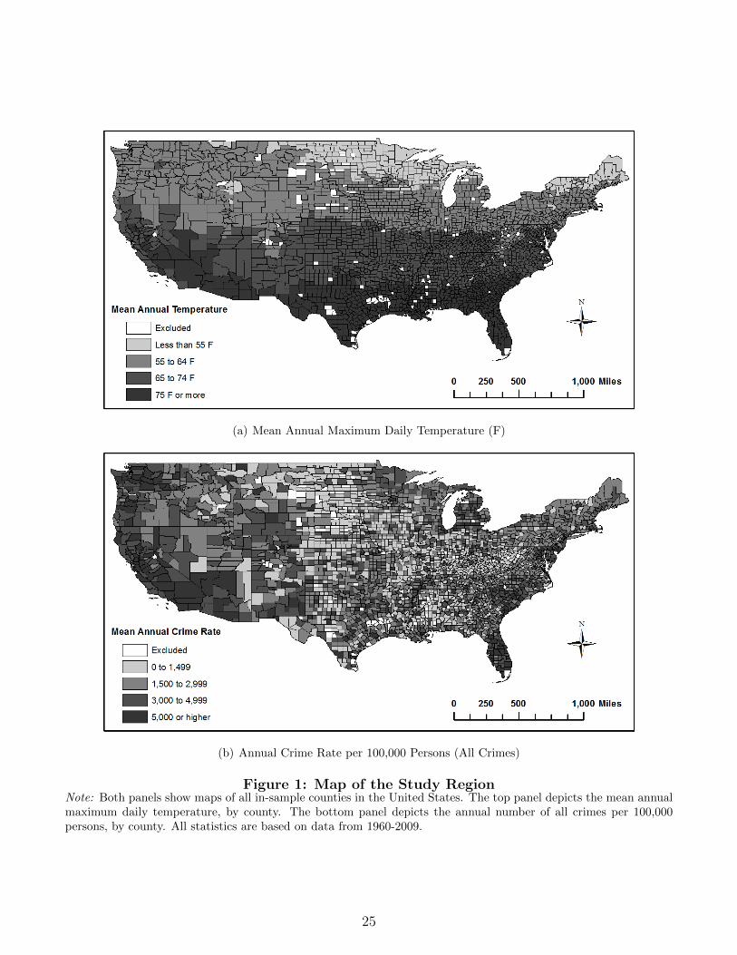
F, 65 to 74 degrees F, and ≥75 degrees F. Panel (a) of Figure 1 shows a map of the climate

zones. As expected, northern areas of the United States are more likely to have cooler climates.

For comparison, Panel (b) of the figure shows a map of county-level annual crime rates per

100,000 persons, for all crimes. The panel shows that crime rates are highest along the Eastern

Seaboard, in the West, and in areas bordering the Great Lakes. However, there is no obvious

cross-sectional relationship between the temperature zones and crime rates.6

6Given the many socioeconomic variables that influence crime, the absence of a strong visual cross-sectionalrelationship between temperatures and crime does not necessarily indicate the lack of a causal relationship. A cross-sectional analysis in the spirit of Mendelsohn, Nordhaus, and Shaw (1994) would have to control for other first-orderdeterminants of crime (e.g., population density).

6

Table 2 summarizes basic characteristics of the crime and weather datasets, by climate zone.

The first panel presents mean annual crime rates per 100,000 persons, by type of offense. The

panel shows that some categories of crime, such as murder, manslaughter, rape, and robbery,

are relatively uncommon. The three categories with the highest rates are larceny, burglary,

and simple assault.

The second panel in Table 2 describes the annual distribution of daily temperatures and

precipitation for in-sample counties. Unlike crime rates, these data show substantial variation

across climate zones. For example, although counties in the coolest climate zone (<55 degrees

F) have an average of only five days per year in which the maximum temperature exceeds 90

degrees F, counties in the warmest climate zone (≥75 degrees F) typically have 85 days per

year with temperatures above 90 degrees F.

The final panel in Table 2 describes county socioeconomic characteristics. The panel shows

that counties in cooler climate zones have fewer minorities and are more likely to be rural.

To illustrate the advantages and challenges of using the UCR crime reporting data, Figure

2 presents the time trend in crime rates for the nine major categories of offenses, by climate

zone. Several main patterns are obvious from the data. First, crime rates increase dramatically

between 1960 and 1980, in some cases by several hundred percent. Given the rapid and

monotonic nature of the this increase, it seems likely that it is driven by increased reporting of

crimes, rather than by changes in underlying criminal behavior. Second, trends across climate

zones appear broadly similar, although there is some heterogeneity in absolute levels. Finally,

there is strong evidence of high frequency variation in crime rates due to seasonality.

Figures 3 and 4 present additional evidence on seasonality in the data. Figure 3 shows the

mean value of daily maximum temperature and daily precipitation, by climate zone and month.

The figure shows strong seasonal patterns in all climate zones, for all variables. Seasonal

variation is largest in the coolest climate zone (<55 degrees F), where the mean temperature

difference between January and July is 60 degrees. For comparison, the seasonal temperature

difference between January and July in the warmest climate zone (≥75 degrees F) is about 35

degrees.

Figure 4 presents similar graphs illustrating how crime rates vary by climate zone and

month. The figure shows that all categories of crime show evidence of seasonality, although

the degree of seasonal variation varies widely across crimes. A few categories of crime, par-

ticularly murder and robbery, show only modest seasonal variation. Other categories, such

as rape, assault, and non-violent property crimes, exhibit strong seasonality. Additionally,

the relationship between seasonality and crime rates variety across climate zones and type of

crimes. For example, larceny and burglary show more pronounced seasonal variation in cooler

climate zones, whereas robbery shows somewhat more seasonality in warmer climates.

7

4 Methodology

The summary statistics from the previous section show a strong correlation between monthly

weather and crime rates. In this section I develop a causal econometric model of this relation-

ship. Specifically, I model crime in month m of year y in county i as follows:

Ciym =

10∑j=1

αj0T

jiym +

5∑k=1

βk0Pkiym

+10∑j=1

αj1T

jiym−1 +

5∑k=1

βk1Pkiym−1

+ φim + θiy + εiym (1)

In this equation, Ciym represents the monthly crime rate per 100,000 residents, φim is a county-

by-month fixed effect, θiy is a county-by-year fixed effect, and εiym is a zero-mean error term.

Following Deschenes and Greenstone (2011), I model the daily distribution of temperatures

within a month using ten bin variables: <10 F, 10-19 F, 20-29 F, 30-39 F, 40-49 F, 50-59 F,

60-69 F, 70-79 F, 80-89 F, and ≥90 F. For example, the variable T jiym represents the number

of days in month m of year y in county c in which the temperature fell into temperature bin

j. I use a similar convention for the precipitation variables P kiym, with five bins: 0 mm, 1-4

mm, 5-14 mm, 15-29 mm, and ≥30 mm. Because of the possibility that changes in crime rates

due to weather shocks may exhibit negative serial correlation (Jacob, Lefgren, and Moretti,

2007), I also include a one month lag of each temperature and precipitation bin variable.

Furthermore, because weather patterns in a particular month are highly correlated between

adjacent geographic areas, I cluster all standard errors at the year-by-month level. I also

weight each county-by-month-by-year observation by the county population in that year.

Equation (1) includes several features designed to address issues that have been prob-

lematic in previous analysis of the effect of weather on criminal behavior. First, by using

a semi-parametric specification for weather, I avoid imposing structural assumptions on the

relationship between weather and crime. Previous analyses have used as independent variables

mean weekly temperature and precipitation (Jacob, Lefgren, and Moretti, 2007) or mean yearly

temperature and temperature squared (Rotton and Cohn, 2003). These specifications assume

that weather has a linear or quadratic effect on crime—which, as the results from this paper

show, may fail to capture important features of the relationship.

Second, Equation (1) includes an extrordinarily comprehensive set of fixed effects. In

addition to including dummy variables for typical monthly patterns in weather and crime

with each county, I include dummy variables that capture the average crime rate and weather

conditions in each county-by-year set of observations. In other words, my identification strategy

is based on only the residual variation in crime and weather remaining between months within

a particular county and year, after controlling for average monthly crime levels.

8

The motivation for this extensive set of fixed effects is related to the quality of the FBI’s

crime data. As Figure 2 illustrates, the UCR crime data exhibit strong interannual trends that

appear to be driven at least partially by differences in reporting. Examination of the microdata

shows that at the level of individual counties, these trends are exacerbated, with crime rates in

many counties jumping wildly from year to year as the set of reporting agencies changes over

time. In the two previous national studies of crime and climate change (Anderson, Bushman,

and Groom, 1997; Rotton and Cohn, 2003), the authors addressed this problem by modeling

annual changes in aggregate national or state crime rates as an autoregressive process. Because

this approach is not an entirely satisfactory method for dealing with measurement error in

the dependent variable, I choose an alternative methodology that requires no consistency in

reporting between years. Instead, as discussed in the data section, I construct monthly crime

rates within each county-by-year by aggregating the total number of reported crimes each

month only for agencies that reported twelve complete months of data for that year. Thus,

although the set of reporting agencies within each county changes between years, making

interannual comparisons invalid except under very strong assumptions, an identical set of

agencies report for each month within a particular year. Thus, the identifying assumption

for my analysis is that after controlling for county-by-year and county-by-month fixed effects,

differences in weather and crime between months within a county represent the true effect of

weather on crime.

5 Results

This section presents the main results from the analysis.

5.1 Weather and Crime Rates

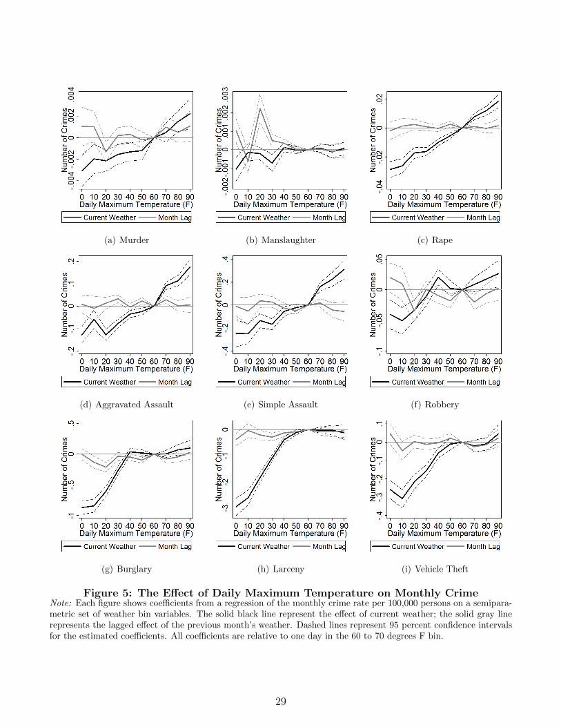
I begin by presenting the regression results from estimating Equation (1). Because of the large

number of coefficients, the results are easiest to understand using a graphical approach. For

example, Figure 5 plots the regression coefficients on the temperature and lagged temperature

bin variables. In each subfigure, the horizontal axis represents the daily maximum temperature

bins, and the vertical axis represents the coefficient, with units of number of crimes per 100,000

persons per month. The figure shows that across all types of crime, higher temperatures cause

statistically significant increases in crime rates. As an illustration, compared to a day in the

60-69 degrees F bin, an extra day in the 30-39 degrees F bin leads to 0.002 fewer murders,

0.08 fewer aggravated assaults, and 1.1 fewer larcenies, per 100,000 persons per month. In

comparison, the mean monthly crime rates for these three offenses are .35 cases of murder,

14 cases of aggravated assult, and 114 cases of larceny. Although the estimated coefficients

appear small relative to mean crime rates, the coefficients represent the effect of only a single

day of weather per month, and in aggregate imply substantial effects. For example, in a spring

9

month with 10 unusually cold days (in the 30-39 degrees F bin), crime rates for these three

offenses would be approximately seven to ten percent lower than crime rates in a spring month

with 10 unusually warm days (in the 60-69 degrees F bin).

Figure 5 also shows the significant non-linearities in the effect of temperatures on crime.

These non-linear effects are most apparent for property crimes such as burglary and larceny.

For bins below 40 degrees F, increases in temperature have a strong positive effect on the

number of burglaries and larcenies reported. However, above 40 degrees F, increases in tem-

perature have little or no effect on these crimes. The degree of nonlinearity varies by offense,

with violent crimes tending to have a much more linear relationship through the entire range

of temperatures.

In addition to showing the effect of current monthly temperatures on current monthly crime,

Figure 5 also presents coefficients and confidence intervals for the effect of lagged temperature

from the previous month. For most offenses, the coefficients on lagged temperatures are close

to zero and not statistically significant. Thus, unlike Jacob, Lefgren, and Moretti (2007), who

find a significant and opposite coefficient on lagged weekly temperatures that dampens the

effect of weather on weekly crime, I conclude that at the monthly level, there is little evidence

that weather has a lagged effect on crime patterns.

Table 3 presents complete regression results from estimating Equation (1), including the

results for the precipitation bin variables. The table shows that the effects of precipition on

crime rates vary by offense. Although precipitation causes statistically significant decreases in

larceny, the opposite is true for vehicle theft: more vehicles are stolen in months with many

rainy days.

One key question about the analytical approach used in this paper is whether one month is

a sufficiently long time period to account for any lagged impacts of weather on crime. Although

the mostly insignificant coefficients on the one-month lag of the weather bins suggest that this

is the case, I also conduct sensitivity analyses in which I run regressions using data that have

been aggregated to quarterly and half-year time periods. Figure 12 in the Appendix shows

the results of this analysis. Although regressions results based on more aggregate time periods

are noisier than the results based on month-long time periods, the estimated coefficients from

the three types of regressions are generally similar. For example, although the relationship

between temperature and crime rates for aggravated and simple assault appears somewhat

weaker based on the quarterly and half-year data, the effect of temperature on burglary and

larceny is even stronger in the quarterly and half-year data. Overall, the figure suggests that

a one-month aggregation period is sufficient to account for “harvesting” that might occur as

a result of negative serial correlation in crime rates.

In addition to the main specifications presented in Figure 5 and Table 3, I have run a variety

of other sensitivity analyses in which I allow the coefficients on the weather bin variables to

vary by climate zone, monthly mean temperature, and decade. The results from these analyses

are qualitatively similar to the main specification presented here, and are presented in the

10

appendix.

5.2 Climate Change and Crime Rates

To assess how climate change is likely to affect crime rates in the United States, I combine the

regression estimates from the previous section with data on simulated U.S. weather conditions

for the time period from 2010 to 2099. These simulations are based on the IPCC’s A1B

scenario, a “middle-of-the-road” climate change scenario that assumes eventual stabilization

of atmospheric CO2 levels at 720 ppm (IPCC, 2000, 2007). I use predictions from two general

circulation models: the U.K. Hadley Centre’s HadCM3 climate model, and the U.S. National

Center for Atmospheric Research’s CCSM3 climate model. The predictions, which are available

from an archive maintained by the World Climate Research Programme’s Coupled Model

Intercomparison Project Phase 3 (CMIP3), have an interpolated resolution of two degrees of

latitude by two degrees of longitude (WCRP, 2007; Maurer et al, 2007).

To use these data to estimate how climate change is likely to affect crime rates in each

county in my analysis, I follow several steps. First, I use the HadCM3 and CCSM3 projections

to calculate average predicted monthly temperature and precipitation for each decade between

2000 and 2099, for each two degree-by-two degree gridpoint. Taking the average monthly

values for 2000-2009 as a baseline, I then calculate the absolute change in mean monthly

temperature and the proportional change in mean monthly precipitation at each gridpoint for

each subsequent decade, relative to 2000-2009. I then assign each U.S. county a predicted

change in temperature and precipitation for each future decade and month, based on the

changes predicted at the closest HadCM3 and CCSM3 gridpoint.

Next, I use these predicted changes to generate a simulated distribution of days across

temperature and precipitation bins for each of the nine decades starting with 2010-2019 and

ending with 2090-2099, for each month and county. I begin with the actual record of tempera-

tures for each day, month, and county between 2000 and 2009. For each decade, I then add the

predicted absolute change in monthly temperature to each daily temperature, by month and

county, yielding a new predicted record of daily temperatures. I generate simulated precipita-

tion data by multiplying the daily precipitation values by the proportional change in predicted

precipitation. I then use these counterfactual weather records to calculate the mean number

of days that will fall into each temperature and precipitation bin in each county and month,

in each future decade. I conduct this procedure separately for the HadCM3 and CCSM3

predictions.

Finally, to predict how the projected change in weather will affect crime rates in each

county, month, and decade, I combine the climate projections with the regression coefficients

estimated in the previous section. I estimate the change in crime rates ∆Cidm in county i,

11

decade d, and month m using the following formula:

∆Cidm = 10 ·[ 10∑j=1

αj0(T̄ j

i,d,m − T̄ ji,2000,m) +

5∑k=1

βk0 (P̄ ki,d,m − P̄ k

i,2000,m)

+

10∑j=1

αj1(T̄ j

i,d,m−1 − T̄ ji,2000,m−1) +

5∑k=1

βk1 (P̄ ki,d,m−1 − P̄ k

i,2000,m−1)]

(2)

where T̄ ji,d,m refers to the mean number of days per month in which the simulated temperature

in month m in county c in decade fell into temperature bin j. The predicted precipitation

variable P̄ ki,d,m−1 is defined similarly. The variables T̄ j

i,2000,m and P̄ ki,2000,m−1 refer to the actual

distribution of days across temperature and precipitation bins during the decade from 2000 to

2009. I multiply the entire expression on the right-hand side of the equation by ten to account

for the number of years in each decade.7

Before discussing the results of this analysis, I present information on the changes in weather

predicted by the CCSM3 and HadCM3 models. Figure 6 shows the distribution of temperature

and precipitation across bins for three scenarios: the actual weather patterns observed between

2000 and 2009, the weather patterns predicted for 2090 to 2099 by the CCSM3 model, and the

weather patterns predicted for 2090 to 2099 by the HadCM3 model. The figure shows that

the baseline (2000-2009) maximum daily temperature distribution is heavily left-skewed. As a

result, the increases in temperatures predicted by the CCSM3 and HadCM3 models lead to a

sharp increase in the number of days that are predicted to fall into the highest daily maximum

temperature bin (≥90 degrees F). The number of days in all other bins decreases under both

sets of model predictions.

Table 4 shows the predicted impacts of climate change on crime in the United States. The

first two columns of the table present estimates of the additional number of crimes that will

occur between 2010 and 2099, compared to the number that would have occurred in the absence

of climate change. The table shows that under both climate models, climate change will cause

a strikingly large number of crimes during the next century. For example, under the HadCM3

model, there will be an additional 35,000 murders, 216,000 cases of rape, 1.6 million aggravated

assaults, 2.4 million simple assaults, 409,000 robberies, 3.1 million burglaries, 3.8 million cases

of larceny, and 1.4 million cases of vehicle theft. All of these changes are significant at the five

percent threshold. The only category of crime that is expected to decrease is manslaughter,

but the expected change is less than 1,000 crimes and is not significantly different from zero.

Compared to the baseline number of crimes expected to occur during this 90 year period in the

absence of climate change, these figures represent a 3.6% increase in murder, a 2.7% decrease

in manslaughter, a 3.8% increase in cases of rape, a 3.1% increase in aggravated assault, a

1.3% increase in simple assault, a 1.6% increase in robbery, a 2.3% increase in burglary, a 0.9%

increase in cases of larceny, and a 1.9% increase in cases of vehicle theft.

7Note that I also adjust ∆Cidm to account for the actual county population.

12

Because these offenses occur over a 90 year time period and include a variety of types of

crimes, it is useful to aggregate them into a social cost metric. I estimate the social costs

of future changes in crime using the following valuations per offense: $5,000,000 for murder

and manslaughter, $41,247 for rape, $19,537 for aggravated assault, $4,884 for simple assault,

$21,398 for robbery, $6,170 for burglary, $3,523 for larceny, and $10,534 for motor vehicle

theft. The social cost estimates for murder and manslaughter are based on the value of a

statistical life (VSL) for workers in U.S. labor markets. Estimates of VSL typically range

between $4 million and $9 million (Viscusi and Aldy, 2003), and I choose $5 million as a

plausible value. Estimates of the social cost of the remaining offences are drawn from a review

article by McCollister, French, and Fang (2010). These valuations represent the tangible costs

of crime, including medical expenses, cash losses, property theft or damage, lost earnings

because of injury, other victimization-related consequences, criminal justice system costs, and

career crime costs.8 Although McCollister, French, and Fang also report intangible costs

of crime (such as pain and suffering), I exclude these estimates because they are based on

jury awards that may not accurately reflect individuals’ actual willingness to pay to avoid

victimization. Exclusion of this category of costs may bias my estimates of the social cost

downward.

The right-hand side of Table 4 shows estimates of the social cost of the climate-related

crime that is likely to occur between 2010 and 2099. Including all offenses, the social costs of

this crime are between $20 billion and $68 billion. Because of the high value of a statistical

life, the costs of future murders are by far the largest component of total social cost. As the

table demonstrates, the estimates are somewhat sensitive to the choice of climate model and

discount rate. For example, based on the HadCM3 model and a three percent discount rate,

the present discounted cost of climate-related murder over the next ninety years is $42 billion.

Based on the CCSM3 model and a six percent discount rate, the social cost of murder is only

$12 billion.

One fact that is not apparent from Table 4 is that the impacts of climate change on crime

are not uniformly distributed across the United States. To investigate distributional effects,

Figure 7 presents—for each U.S. county—the per capita present discounted value of the total

social costs of future climate-related crime, by county. In other words, the figure shows the

discounted value of the social cost of the number of additional crimes expect to occur in each

county over the next 90 years, divided by each county’s current population. The table shows

that the per capita cost of climate-related crime is highest in the West, where costs are between

$140 and $180 per person, and lowest in the South and East, where costs are less than $80 per

person.

8McCollister, French, and Fang (2010) do not report estimates of the social cost of simple assault. For the purposesof this analysis, I value each case of simple assault at 25 percent of the cost of a case of aggravated assault.

13

6 Discussion

The previous sections highlight two main results. First, weather has a strong causal effect on

the incidence of criminal activity. For all offenses except manslaughter, higher temperatures

lead to higher crime rates. The functional form of the relationship varies across offenses, with

some categories, particularly property crimes, showing largest marginal effects below 40 degrees

F. This low-temperature dependency is in some ways surprising. Analyses of the impact of

climate change on other economic outcomes, such as agriculture, have highlighted the role of

extremely warm temperatures (Schlenker and Roberts, 2009). In contrast, my results suggest

that the impact of climate change on property crime may operate largely through changes in

the frequency of days with low to moderate temperatures.

Second, climate change will cause a substantial increase in crime in the United States.

Relative to the total number of offenses that would occur between 2010 and 2099 in the

absence of climate change, my calculations suggest that there will be an additional 35,000

murders, 216,000 cases of rape, 1.6 million aggravated assaults, 2.4 million simple assaults,

409,000 robberies, 3.1 million burglaries, 3.8 million cases of larceny, and 1.4 million cases of

vehicle theft. The present discounted value of the social costs of these climate-related crimes

is between 20 and 68 billion dollars.9

In interpreting these results, it is important to keep in mind that climate change will

affect humans in a variety of ways (Tol, 2009; Deschenes and Greenstone, 2007, 2011; Hsiang,

Meng, and Cane, 2011), and that a comprehensive cost-benefit analysis of climate change

should consider all dimensions of costs and benefits. For example, given U.S. residents’ high

willingness to pay to live in areas with moderate climates (Cragg and Kahn, 1996), it is possible

that the social costs of increased crime will be offset, at least in some regions, by the social

benefits of more pleasant weather.

It is also worth emphasizing that the estimates presented here do not take into account

longer-term adaptation mechanisms. If climate change does cause a permanent increase in the

frequency of crime, people in affected areas will have the opportunity to modify their behavior

to avoid being victimized. Furthermore, it is likely that law enforcement agencies will respond

with increased policing activity. The potential for such actions suggests that the estimates in

this paper should be viewed as an upper bound on the potential impacts of climate change on

crime.

The estimates in this paper also assume a static baseline of criminal activity, based on

9To put these dollar values in context, Deschenes and Greenstone (2011) estimate that climate-related changesin mortality and energy consumption will cause welfare losses of $892 billion over the next century, based on a 3%discount rate and the HadCM3 model’s predictions for the A1F1 scenario. Differencing out my estimate of themortality-related costs of crime (murder and manslaughter together have a cost of approximately $41 billion) impliesthat crime-related costs ($68 billion) are likely to be about eight percent as large as the energy consumption andnon-crime-related mortality costs of climate change in the United States ($851). Of course, this comparison ignoresany differences between the A1F1 and A1B emissions scenarios (the A1F1 scenario assumes higher emissions andmore warming than the A1B scenario used in this paper).

14

average crime rates between 2000 and 2009. Given the challenges of accurately predicting

long-term trends in crime rates (Levitt, 2004), such an assumption is a reasonable analytical

strategy. However, if for reasons unrelated to climate change, crime rates were to increase

or decrease substantially over the coming decades, then the estimates from this paper could

significantly over- or underestimate climate’s effects on future crime.

As a final caveat, I emphasize that this paper’s estimates of the social cost of climate-related

crime should be considered to be highly uncertain. Although I monetize the social costs of

additional crimes using point estimates drawn from the VSL and crime literatures (Viscusi

and Aldy, 2003; McCollister, French, and Fang, 2010), I make no attempt to characterize the

range of uncertainties associated with these valuations. Furthermore, consistent with previous

literature on the role of discounting in economic analysis of climate change (Weitzman, 2007),

I find that the present value of the social costs of additional crime depends heavily on the

choice of a discount rate. Thus, the costs presented here are best interpreted as “back-of-

the-envelope” estimates, rather than as precise statements of the exact cost of climate-related

crime.

7 Conclusion

In this paper, I document a robust statistical relationship between historical weather patterns

and criminal activity, and use this relationship to predict how changes in U.S. climate will

affect future patterns of criminal behavior. The results suggest that climate change will have

substantial effects on the prevalence of crime in the United States. Although previous assess-

ments of the costs and benefits of climate change have primarily focused on other economic

endpoints, the magnitude of the estimated impacts from this paper suggests that changes in

crime are an important component of the broader impacts of climate change.

15

8 Appendix

This appendix presents the results of a variety of sensitivity analyses of the relationship between

weather and crime.

One potential concern about the analysis is that the relationship between weather and

crime may have changed over time. To address this concern, Figure 8 plots the coefficients

from separate regressions based on each of the five decades covered by the data: 1960-1969,

1970-1979, 1980-1989, 1990-1999, and 2000-2009. The data show more noise than the main

regression results, but the overall pattern of crime increasing with temperature remains similar

across decades for almost all crimes.

A second potential question is related to long-term adaptation. In particular, if residents

of warmer climates are better adapted to warmer temperatures, then the relationship between

weather and crime may vary across geographic regions. To assess whether this is the case,

Figure 9 shows the results from separate regressions for counties in each of the four climate

zones (based on long-term mean annual maximum daily temperature): <55 degrees F, 55 to

64 degrees F, 65 to 74 degrees F, and ≥75 degrees F. The figure shows that the effects of

moderate and warm temperatures on crime is strikingly similar across climate zones. For very

cold temperatures, the coefficients show somewhat more divergence, but this imprecision is

primarily due to the fact that there are few days in the dataset in which the warmest climate

zones are exposed to very low temperatures.

Another possibility related to adaptation is that people adjust to seasonal conditions, so

that crime rates are driven by weather conditions relative to local expectations for that time of

year. Under this hypothesis, a 60 degree F day could have very different effects depending on

whether it occured in April or July. As a test of this supposition, Figure 10 presents the results

of a regression that includes interactions of the weather bin coefficients with three county-

month temperature category variables. These categorical dummy variables indicate whether

the average temperature in each month-by-county, over the period from 1960 to 2009, fell into

one of three bins: <45 degrees F, 45 to 69 degrees F, or ≥70 F. Although the regressions show

a fair amount of noise, particularly for temperatures that are not typical of normal monthly

conditions, there are no obvious differences in the effects of temperature on crime that can be

attributed to seasonal adaptation.

One additional concern about the analysis is related to heteroskedasticity in the crime rate

variables. There is a large degree of variation in absolute crime levels between counties, and

plots of time trends for individual counties show that the degree of seasonal variation is roughly

proportional to the magnitude of the crime rate. Unfortunately, because the data contain a

large number of months in which no crimes were comitted (particularly for violent offenses

such as murder and manslaughter), using a log transformation would be an inappropriate way

to deal with this heteroskedasticity. Instead, as a sensitivity analysis, I estimate separate

regressions for counties in each of four crime quartiles. To construct the quartiles, I calculate

16

the mean crime rate for total crimes for each in-sample county, averaging across months and

years. I then order these mean crime rates from highest to lowest. Quartile 1 represents

counties below the 25th percentile; Quartile 2 represents counties between the 25 and 49th

percentiles; Quartile 3 represents counties between the 50 and 74th percentiles; and Quartile

4 represents counties at or above the 75th percentile.

Figure 11 shows the results from this analysis. Generally speaking, the coefficients from

Quartiles 1, 2, and 3 are of similar magnitude. As expected, the coefficients from regressions

using data from Quartile 4 (counties with the highest average crime rate for all crimes) tend

to be larger, although the exact degree of difference varies across types of crime.

A final question about the analytical approach used in this paper is whether one month is a

sufficiently long time period to account for any lagged impacts of weather on crime. Although

the insignificant coefficients on a one-month lag of weather suggest this is the case, I also

conduct sensitivity analyses in which I run regressions using data that have been aggregated

to quarterly and half-year time periods. Figure 12 shows the results of this analysis. Although

regressions results based on more aggregate time periods are noisier than the results based

on month-long time periods, the estimated coefficients from the three types of regressions are

generally similar. The relationship between temperature and crime rates for aggravated and

simple assault appears somewhat weaker based on the quarterly and half-year data. However,

the effect of temperature on burglary and larceny is even stronger in the quarterly and half-

year data. Overall, the figure suggests that a one-month aggregation period is sufficient to

account for most “harvesting” that occurs as a result of negative serial correlation in crime

rates.

References

Agnew, Robert. 2012. “Dire forecast: A Theoretical Model of the Impact of Climate

Change on Crime.” Theoretical Criminology 16(1): 21.

Anderson, Craig. 1989. “Temperature and Aggression: Ubiquitous Effects of Heat on

Occurrence of Human Violence.” Psychological Bulletin 106(1): 74-96.

Anderson, Craig, Brad Bushman, and Ralph Groom. 1997. “Hot Years and Serious and

Deadly Assault: Empirical Tests of the Heat Hypothesis.” Journal of Personality and

Social Psychology 73(6): 1213-1223.

Baumeister, Roy, and Todd Heatherton. 1996. “Self Regulation Failure: An Overview.”

Psychological Inquiry 7(1): 1-15.

Baron, Robert, and Paul Bell. 1976. “Aggression and Heat: The Influence of Ambient

Temperature, Negative Affect, and a Cooling Drink on Physical Aggression.” Journal of

Personality and Social Psychology 33(3): 245-255.

17

Becker, Gary. 1968. “Crime and Punishment: An Economic Approach.” Journal of

Political Economy 76: 169-217.

Brunsdon, Chris, Jonathan Corcoran, Gary Higgs, and Andrew Ware. 2009. “The Influ-

ence of Weather on Local Geographical Patterns of Police Calls for Service.” Environment

and Planning B: Planning and Design 36(5): 906-926.

Bushman, Brad, Morgan Wang, and Craig Anderson. 2005. “Is the Curve Relating

Temperature to Aggression Linear or Curvilinear?” Journal of Personality and Social

Psychology 89(1): 62-66.

Card, David, and Gordon Dahl. 2011. “Family Violence and Football: The Effect of

Unexpected Emotional Cues on Violent Behavior.” Quarterly Journal of Economics

126(4): 1879-1907.

Cohn, Ellen. 1990. “Weather and Crime.” British Journal of Criminology 30(1): 51-64.

Cohn, Ellen, and James Rotton. 2000. “Weather, Seasonal Trends, and Property Crimes

in Minneapolis, 1987-1988: A Moderator-Variable Time-Series Analysis of Routine Ac-

tivities.” Journal of Environmental Psychology 20(3): 257-272.

Cragg, Michael, and Matthew Kahn. 1997. “New Estimates of Climate Demand: Evi-

dence from Location Choice.” Journal of Urban Economics 42: 261-284.

Deschenes, Olivier, and Michael Greenstone. 2007. “The Economic Impacts of Climate

Change: Evidence from Agricultural Output and Random Fluctuations in Weather.”

American Economic Review. March.

Deschenes, Olivier, and Michael Greenstone. 2011. “Climate Change, Mortality, and

Adaptation: Evidence from Annual Fluctuations in Weather in the US.” American Eco-

nomic Journal: Applied Economics 3(4): 152185.

Federal Bureau of Investigation (FBI). 2004. “Uniform Crime Reporting Handbook.”

http://www.fbi.gov/about-us/cjis/ucr/additional-ucr-publications/ucr_handbook.

pdf. Accessed March 8, 2012.

Federal Bureau of Investigation (FBI). 2011a. “Uniform Crime Reporting Data, Return

A and Supplement to Return A.” Compact disc, obtained from the FBI’s Multimedia

Productions Group.

Federal Bureau of Investigation (FBI). 2011b. “Crime in the United States, 2010: About

the Uniform Crime Reporting Program.” http://www.fbi.gov/about-us/cjis/ucr/

crime-in-the-u.s/2010/crime-in-the-u.s.-2010/aboutucrmain.pdf. Accessed March

8, 2012.

Glaeser, Edward, Bruce Sacerdote, and Jose Scheinkman. 1996. “Crime and Social

Interactions.” Quarterly Journal of Economics 111(2): 507-48.

18

Hsiang, Solomon, Kyle Meng, and Mark Cane. 2011. “Civil Conflicts Are Associated

with the Global Climate.” Nature 476: 438-441.

Intergovernmental Panel on Climate Change (IPCC). 2000. “IPCC Special Report:

Emissions Scenarios.” Available at http://www.ipcc.ch/pdf/special-reports/spm/

sres-en.pdf.

Intergovernmental Panel on Climate Change (IPCC). 2007. “Working Group I: The

Physical Science Basis.” Fourth Assessment Report: Climate Change 2007.

Jacob, Brian, Lars Lefgren, and Enrico Moretti. 2007. “The Dynamics of Criminal

Behavior: Evidence from Weather Shocks.” Journal of Human Resources 42(3): 489-

527.

Levitt, Steven. 1996. “The Effect of Prison Population Size on Crime Rates: Evidence

from Prison Overcrowding Litigation.” Quarterly Journal of Economics 111(2): 319-351.

Levitt, Steven. 2004. “Understanding Why Crime Fell in the 1990s: Four Factors that

Explain the Decline and Six that Do Not.” Journal of Economic Perspectives 18(1):

163190.

Maurer, E. P., L. Brekke, T. Pruitt, and P. B. Duffy. 2007. “Fine-resolution climate pro-

jections enhance regional climate change impact studies.” Eos, Transactions, American

Geophysical Union 88(47): 504.

Mendelsohn, Robert, William Nordhaus, and Daigee Shaw. 1994. “The Impact of Global

Warming on Agriculture: A Ricardian Analysis.” The American Economic Review 84(4):

753-771.

McCollister, Kathryn, Michael French, and Hai Fang. 2010. “The Cost of Crime to

Society: New Crime-specific Estimates for Policy and Program Evaluation.” Drug and

Alcohol Dependence 108(1-2): 98-109.

National Climatic Data Center (NCDC) Climate Services Branch. 2011. “Global His-

torical Climatology Network – Daily.” Available at http://www.ncdc.noaa.gov/oa/

climate/ghcn-daily/. Accessed 4/28/2011.

Rotton, James, and Ellen Cohn. 2003. “Global Warming and U.S. Crime Rates: An

Application of Routine Activity Theory.” Environment and Behavior 35(6): 802-825.

Schlenker, Wolfram, and Michael Roberts. 2009. “Nonlinear Temperature Effects Indi-

cate Severe Damages to U.S. Crop Yields under Climate Change.” Proceedings of the

National Academy of Sciences 106(37): 15594-15598.

Simister, John. 2002. “Thermal Stress and Violence in India and Pakistan: Investigating

a New Explanation of the Kerala Model.” Development Ideas and Practices Working

Paper DIP-02-01.

19

Simister, John, and Cary Cooper. 2005. “Thermal Stress in the USA: Effects on Violence

and on Employee Behavior.” Stress and Health 21: 315.

Simister, John, and Evert Van de Vliert. 2005. “Is There More Violence in Very Hot

Weather? Tests over Time in Pakistan and Across Countries Worldwide.’ Pakistan

Journal of Meteorology 2(4): 55-70.

Tol, Richard. 2009. “The Economic Effects of Climate Change.” Journal of Economic

Perspectives 23(2): 29-51.

U.S. Census Bureau. 1978. “Consolidated File: County and City Data Book.” ICPSR:

Washington, DC. Available at http://www.icpsr.umich.edu/icpsrweb/ICPSR/studies/

07736. Accessed May 10, 2011.

U.S. Census Bureau. 2004. “Intercensal County Estimates by Age, Sex, Race: 1970-

1979, 1980-1989, 1990-1999.” Available at http://www.census.gov/popest/archives/

pre-1980/co-asr-7079.html, http://www.census.gov/popest/archives/1980s/PE-02.

html, and http://www.census.gov/popest/datasets.html#cntyinter. Accessed May

7, 2011.

U.S. Census Bureau. 2011. “Annual Estimates of the Resident Population by Age,

Sex, Race, and Hispanic Origin for Counties: April 1, 2000 to July 1, 2009.” Avail-

able at http://www.census.gov/popest/counties/asrh/CC-EST2009-alldata.html.

Accessed May 7, 2011.

Viscusi, W. Kip, and Joseph Aldy. 2003. “The Value of a Statistical Life: A Critical

Review of Market Estimates Throughout the World.” Journal of Risk and Uncertainty

27(1): 5-76.

Weitzman, Martin. 2007. “A Review of The Stern Review on the Economics of Climate

Change.” Journal of Economic Literature 45(3): 703-724.

World Climate Research Programme (WCRP). 2007. “Coupled Model Intercomparison

Project Phase 3 (CMIP3) Multi-model Dataset.” Available from the “Bias Corrected and

Downscaled WCRP CMIP3 Climate Projections” archive at http://gdo-dcp.ucllnl.

org/downscaled_cmip3_projections/. Accessed March 10, 2012. 10

10I acknowledge the modeling groups, the Program for Climate Model Diagnosis and Intercomparison, the WCRP’sWorking Group on Coupled Modeling, and the U.S. Department of Energy Office of Science for their roles in makingavailable and supporting the WCRP CMIP3 multi-model dataset.

20

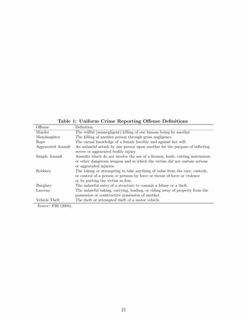
Table 1: Uniform Crime Reporting Offense DefinitionsOffense DefinitionMurder The willful (nonnegligent) killing of one human being by another.Manslaughter The killing of another person through gross negligence.Rape The carnal knowledge of a female forcibly and against her will.Aggravated Assault An unlawful attack by one person upon another for the purpose of inflicting

severe or aggravated bodily injury.Simple Assault Assaults which do not involve the use of a firearm, knife, cutting instrument,

or other dangerous weapon and in which the victim did not sustain seriousor aggravated injuries.

Robbery The taking or attempting to take anything of value from the care, custody,or control of a person or persons by force or threat of force or violenceor by putting the victim in fear.

Burglary The unlawful entry of a structure to commit a felony or a theft.Larceny The unlawful taking, carrying, leading, or riding away of property from the

possession or constructive possession of another.Vehicle Theft The theft or attempted theft of a motor vehicle.

Source: FBI (2004).

21

Table 2: Summary Statistics, by Climate ZoneMean Annual Maximum Daily Temperature

<55 F 55-64 F 65-74 F ≥75 F

Monthly Crime Rate (per 100,000 persons)Murder 0.1 (1.2) 0.2 (1.3) 0.4 (1.9) 0.6 (2.2)Manslaughter 0.03 (0.53) 0.03 (0.50) 0.02 (0.45) 0.02 (0.42)Rape 1.2 (3.5) 1.2 (3.2) 1.3 (3.3) 1.6 (3.5)Aggravated Assault 6 (13) 9 (14) 15 (20) 20 (22)Simple Assault 26 (40) 31 (39) 34 (48) 41 (52)Robbery 1 (3) 2 (5) 3 (6) 4 (8)Burglary 43 (48) 44 (45) 50 (46) 61 (53)Larceny 111 (94) 117 (98) 107 (97) 125 (112)Vehicle Theft 9 (12) 11 (15) 11 (15) 13 (18)

Annual Number of Days in Weather BinMax Temp: <10 F 13 (11) 3 (4) 0 (1) 0 (0)Max Temp: 10-19 F 20 (8) 7 (6) 1 (2) 0 (0)Max Temp: 20-29 F 37 (9) 20 (11) 5 (5) 0 (1)Max Temp: 30-39 F 52 (12) 44 (14) 18 (11) 3 (4)Max Temp: 40-49 F 41 (11) 49 (14) 35 (12) 12 (8)Max Temp: 50-59 F 40 (9) 49 (16) 50 (11) 31 (13)Max Temp: 60-69 F 49 (11) 52 (13) 59 (13) 54 (13)Max Temp: 70-79 F 64 (11) 64 (14) 68 (14) 77 (14)Max Temp: 80-89 F 43 (14) 63 (18) 86 (18) 101 (28)Max Temp: ≥90 F 6 (8) 15 (14) 43 (25) 86 (29)Precip: 0 mm 179 (47) 165 (44) 196 (40) 215 (46)Precip: 1-4 mm 143 (37) 149 (34) 111 (29) 95 (30)Precip: 5-14 mm 32 (11) 37 (14) 36 (12) 33 (14)Precip: 15-29 mm 9 (4) 11 (6) 15 (7) 15 (7)Precip: ≥30 mm 2 (2) 3 (3) 6 (4) 8 (5)

County CharacteristicsPopulation 36,289 (51,843) 96,286 (246,799) 71,616 (316,927) 86,742 (237,757)Pct White 97 (8) 96 (6) 87 (16) 78 (18)Pct Female 50 (1) 51 (1) 51 (2) 51 (2)Pct Ages 0-4 7 (2) 7 (1) 7 (1) 8 (1)Pct Ages 5-19 25 (5) 25 (4) 25 (4) 26 (5)Pct Ages 65-up 15 (4) 14 (4) 13 (4) 13 (5)Pct Metro Center 2 (15) 7 (26) 6 (24) 4 (20)Pct Metropolitan 14 (35) 24 (43) 22 (41) 27 (44)Pct Urban 54 (50) 50 (50) 50 (50) 56 (50)Pct Rural 30 (46) 19 (40) 22 (41) 13 (33)Counties 209 1,092 1,141 530Complete County Years 9,183 48,288 45,544 18,954County Month Obs. 110,196 579,456 546,528 227,448

Note: The table shows mean crime rates, weather conditions, and socioeconomic characteristics forall in-sample counties for the years 1960-2009. Numbers in parentheses indicate standard deviations.Results are presented separately for counties in each of four climate zones, based on mean annualmaximum daily temperature.

22

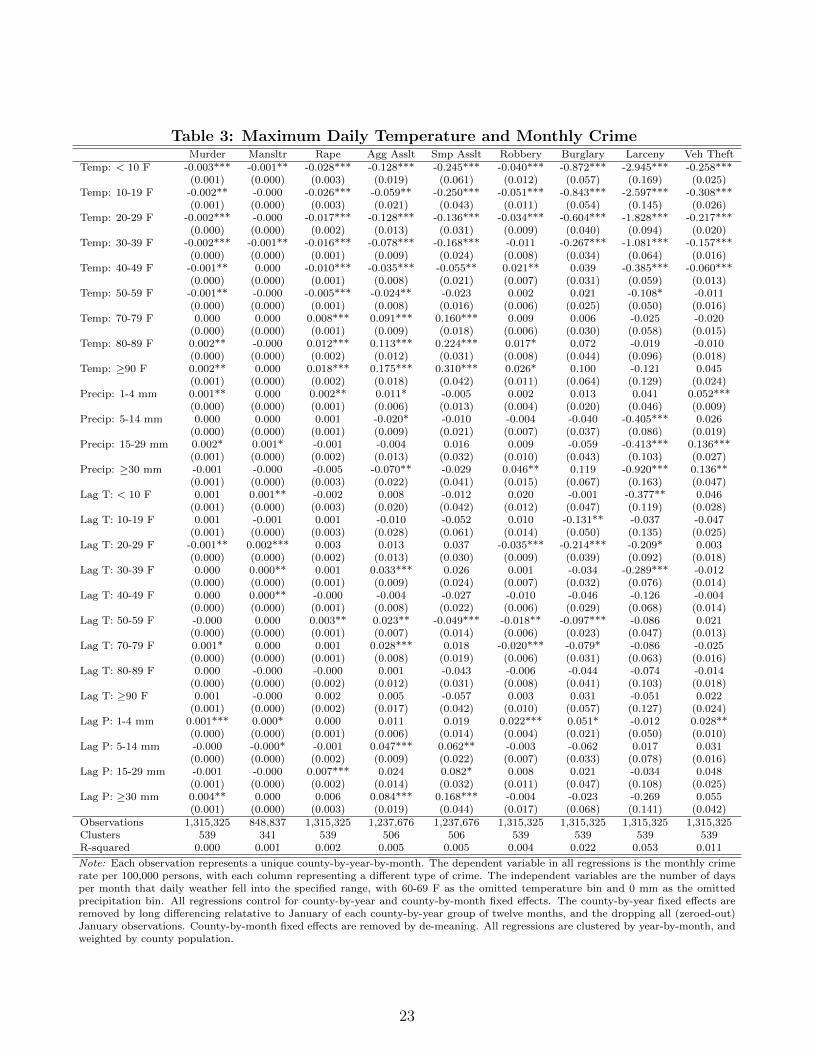
Table 3: Maximum Daily Temperature and Monthly CrimeMurder Mansltr Rape Agg Asslt Smp Asslt Robbery Burglary Larceny Veh Theft

Temp: < 10 F -0.003*** -0.001** -0.028*** -0.128*** -0.245*** -0.040*** -0.872*** -2.945*** -0.258***(0.001) (0.000) (0.003) (0.019) (0.061) (0.012) (0.057) (0.169) (0.025)

Temp: 10-19 F -0.002** -0.000 -0.026*** -0.059** -0.250*** -0.051*** -0.843*** -2.597*** -0.308***(0.001) (0.000) (0.003) (0.021) (0.043) (0.011) (0.054) (0.145) (0.026)

Temp: 20-29 F -0.002*** -0.000 -0.017*** -0.128*** -0.136*** -0.034*** -0.604*** -1.828*** -0.217***(0.000) (0.000) (0.002) (0.013) (0.031) (0.009) (0.040) (0.094) (0.020)

Temp: 30-39 F -0.002*** -0.001** -0.016*** -0.078*** -0.168*** -0.011 -0.267*** -1.081*** -0.157***(0.000) (0.000) (0.001) (0.009) (0.024) (0.008) (0.034) (0.064) (0.016)

Temp: 40-49 F -0.001** 0.000 -0.010*** -0.035*** -0.055** 0.021** 0.039 -0.385*** -0.060***(0.000) (0.000) (0.001) (0.008) (0.021) (0.007) (0.031) (0.059) (0.013)

Temp: 50-59 F -0.001** -0.000 -0.005*** -0.024** -0.023 0.002 0.021 -0.108* -0.011(0.000) (0.000) (0.001) (0.008) (0.016) (0.006) (0.025) (0.050) (0.016)

Temp: 70-79 F 0.000 0.000 0.008*** 0.091*** 0.160*** 0.009 0.006 -0.025 -0.020(0.000) (0.000) (0.001) (0.009) (0.018) (0.006) (0.030) (0.058) (0.015)

Temp: 80-89 F 0.002** -0.000 0.012*** 0.113*** 0.224*** 0.017* 0.072 -0.019 -0.010(0.000) (0.000) (0.002) (0.012) (0.031) (0.008) (0.044) (0.096) (0.018)

Temp: ≥90 F 0.002** 0.000 0.018*** 0.175*** 0.310*** 0.026* 0.100 -0.121 0.045(0.001) (0.000) (0.002) (0.018) (0.042) (0.011) (0.064) (0.129) (0.024)

Precip: 1-4 mm 0.001** 0.000 0.002** 0.011* -0.005 0.002 0.013 0.041 0.052***(0.000) (0.000) (0.001) (0.006) (0.013) (0.004) (0.020) (0.046) (0.009)

Precip: 5-14 mm 0.000 0.000 0.001 -0.020* -0.010 -0.004 -0.040 -0.405*** 0.026(0.000) (0.000) (0.001) (0.009) (0.021) (0.007) (0.037) (0.086) (0.019)

Precip: 15-29 mm 0.002* 0.001* -0.001 -0.004 0.016 0.009 -0.059 -0.413*** 0.136***(0.001) (0.000) (0.002) (0.013) (0.032) (0.010) (0.043) (0.103) (0.027)

Precip: ≥30 mm -0.001 -0.000 -0.005 -0.070** -0.029 0.046** 0.119 -0.920*** 0.136**(0.001) (0.000) (0.003) (0.022) (0.041) (0.015) (0.067) (0.163) (0.047)

Lag T: < 10 F 0.001 0.001** -0.002 0.008 -0.012 0.020 -0.001 -0.377** 0.046(0.001) (0.000) (0.003) (0.020) (0.042) (0.012) (0.047) (0.119) (0.028)

Lag T: 10-19 F 0.001 -0.001 0.001 -0.010 -0.052 0.010 -0.131** -0.037 -0.047(0.001) (0.000) (0.003) (0.028) (0.061) (0.014) (0.050) (0.135) (0.025)

Lag T: 20-29 F -0.001** 0.002*** 0.003 0.013 0.037 -0.035*** -0.214*** -0.209* 0.003(0.000) (0.000) (0.002) (0.013) (0.030) (0.009) (0.039) (0.092) (0.018)

Lag T: 30-39 F 0.000 0.000** 0.001 0.033*** 0.026 0.001 -0.034 -0.289*** -0.012(0.000) (0.000) (0.001) (0.009) (0.024) (0.007) (0.032) (0.076) (0.014)

Lag T: 40-49 F 0.000 0.000** -0.000 -0.004 -0.027 -0.010 -0.046 -0.126 -0.004(0.000) (0.000) (0.001) (0.008) (0.022) (0.006) (0.029) (0.068) (0.014)

Lag T: 50-59 F -0.000 0.000 0.003** 0.023** -0.049*** -0.018** -0.097*** -0.086 0.021(0.000) (0.000) (0.001) (0.007) (0.014) (0.006) (0.023) (0.047) (0.013)

Lag T: 70-79 F 0.001* 0.000 0.001 0.028*** 0.018 -0.020*** -0.079* -0.086 -0.025(0.000) (0.000) (0.001) (0.008) (0.019) (0.006) (0.031) (0.063) (0.016)

Lag T: 80-89 F 0.000 -0.000 -0.000 0.001 -0.043 -0.006 -0.044 -0.074 -0.014(0.000) (0.000) (0.002) (0.012) (0.031) (0.008) (0.041) (0.103) (0.018)

Lag T: ≥90 F 0.001 -0.000 0.002 0.005 -0.057 0.003 0.031 -0.051 0.022(0.001) (0.000) (0.002) (0.017) (0.042) (0.010) (0.057) (0.127) (0.024)

Lag P: 1-4 mm 0.001*** 0.000* 0.000 0.011 0.019 0.022*** 0.051* -0.012 0.028**(0.000) (0.000) (0.001) (0.006) (0.014) (0.004) (0.021) (0.050) (0.010)

Lag P: 5-14 mm -0.000 -0.000* -0.001 0.047*** 0.062** -0.003 -0.062 0.017 0.031(0.000) (0.000) (0.002) (0.009) (0.022) (0.007) (0.033) (0.078) (0.016)

Lag P: 15-29 mm -0.001 -0.000 0.007*** 0.024 0.082* 0.008 0.021 -0.034 0.048(0.001) (0.000) (0.002) (0.014) (0.032) (0.011) (0.047) (0.108) (0.025)

Lag P: ≥30 mm 0.004** 0.000 0.006 0.084*** 0.168*** -0.004 -0.023 -0.269 0.055(0.001) (0.000) (0.003) (0.019) (0.044) (0.017) (0.068) (0.141) (0.042)

Observations 1,315,325 848,837 1,315,325 1,237,676 1,237,676 1,315,325 1,315,325 1,315,325 1,315,325Clusters 539 341 539 506 506 539 539 539 539R-squared 0.000 0.001 0.002 0.005 0.005 0.004 0.022 0.053 0.011

Note: Each observation represents a unique county-by-year-by-month. The dependent variable in all regressions is the monthly crimerate per 100,000 persons, with each column representing a different type of crime. The independent variables are the number of daysper month that daily weather fell into the specified range, with 60-69 F as the omitted temperature bin and 0 mm as the omittedprecipitation bin. All regressions control for county-by-year and county-by-month fixed effects. The county-by-year fixed effects areremoved by long differencing relatative to January of each county-by-year group of twelve months, and the dropping all (zeroed-out)January observations. County-by-month fixed effects are removed by de-meaning. All regressions are clustered by year-by-month, andweighted by county population.

23

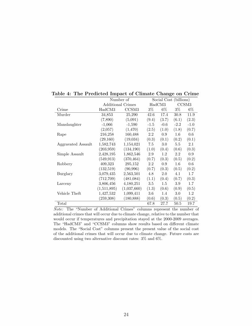
Table 4: The Predicted Impact of Climate Change on CrimeNumber of Social Cost (billions)

Additional Crimes HadCM3 CCSM3Crime HadCM3 CCSM3 3% 6% 3% 6%Murder 34,853 25,290 42.6 17.4 30.8 11.9

(7,890) (5,091) (9.4) (3.7) (6.1) (2.3)Manslaughter -1,066 -1,590 -1.5 -0.6 -2.2 -1.0

(2,057) (1,470) (2.5) (1.0) (1.8) (0.7)Rape 216,258 160,488 2.2 0.9 1.6 0.6

(29,160) (19,034) (0.3) (0.1) (0.2) (0.1)Aggravated Assault 1,582,743 1,154,021 7.5 3.0 5.5 2.1

(203,959) (134,190) (1.0) (0.4) (0.6) (0.3)Simple Assault 2,428,195 1,862,546 2.9 1.2 2.2 0.9

(549,913) (370,464) (0.7) (0.3) (0.5) (0.2)Robbery 409,323 295,152 2.2 0.9 1.6 0.6

(132,519) (90,996) (0.7) (0.3) (0.5) (0.2)Burglary 3,079,435 2,563,501 4.8 2.0 4.1 1.7

(712,709) (481,084) (1.1) (0.4) (0.7) (0.3)Larceny 3,806,456 4,180,251 3.5 1.5 3.9 1.7

(1,511,895) (1,037,660) (1.3) (0.6) (0.9) (0.5)Vehicle Theft 1,427,532 1,099,411 3.6 1.4 3.0 1.2

(259,308) (180,888) (0.6) (0.3) (0.5) (0.2)Total 67.8 27.7 50.5 19.7

Note: The “Number of Additional Crimes” columns represent the number ofadditional crimes that will occur due to climate change, relative to the number thatwould occur if temperatures and precipitation stayed at the 2000-2009 averages.The “HadCM3” and “CCSM3” columns show results based on different climatemodels. The “Social Cost” columns present the present value of the social costof the additional crimes that will occur due to climate change. Future costs arediscounted using two alternative discount rates: 3% and 6%.

24

(a) Mean Annual Maximum Daily Temperature (F)

(b) Annual Crime Rate per 100,000 Persons (All Crimes)

Figure 1: Map of the Study RegionNote: Both panels show maps of all in-sample counties in the United States. The top panel depicts the mean annualmaximum daily temperature, by county. The bottom panel depicts the annual number of all crimes per 100,000persons, by county. All statistics are based on data from 1960-2009.

25

(a) Murder (b) Manslaughter (c) Rape

(d) Aggravated Assault (e) Simple Assault (f) Robbery

(g) Burglary (h) Larceny (i) Vehicle Theft

Figure 2: Crime Rate Trends, by Climate ZoneNote: Each panel shows the mean crime rate across counties within each climate zone, by year and month. Thecrime rate variables represent the monthly number of crimes per 100,000 persons.

26

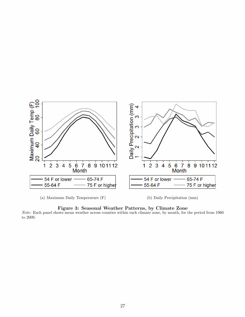
(a) Maximum Daily Temperature (F) (b) Daily Precipitation (mm)

Figure 3: Seasonal Weather Patterns, by Climate ZoneNote: Each panel shows mean weather across counties within each climate zone, by month, for the period from 1960to 2009.

27

(a) Murder (b) Manslaughter (c) Rape

(d) Aggravated Assault (e) Simple Assault (f) Robbery

(g) Burglary (h) Larceny (i) Vehicle Theft

Figure 4: Seasonal Crime Rate Trends, by Climate ZoneNote: Each panel shows the mean crime rate across counties within each climate zone, by month. The crime ratevariables represent the monthly number of crimes per 100,000 persons.

28

(a) Murder (b) Manslaughter (c) Rape

(d) Aggravated Assault (e) Simple Assault (f) Robbery

(g) Burglary (h) Larceny (i) Vehicle Theft

Figure 5: The Effect of Daily Maximum Temperature on Monthly CrimeNote: Each figure shows coefficients from a regression of the monthly crime rate per 100,000 persons on a semipara-metric set of weather bin variables. The solid black line represent the effect of current weather; the solid gray linerepresents the lagged effect of the previous month’s weather. Dashed lines represent 95 percent confidence intervalsfor the estimated coefficients. All coefficients are relative to one day in the 60 to 70 degrees F bin.

29

(a) Maximum Daily Temperature (F) (b) Daily Precipitation (mm)

Figure 6: Distribution of Daily Weather, by ScenarioNote: Each panel shows the number of days per month that fall into the specified weather bin.

30

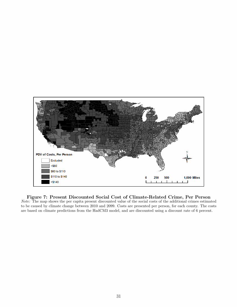
Figure 7: Present Discounted Social Cost of Climate-Related Crime, Per PersonNote: The map shows the per capita present discounted value of the social costs of the additional crimes estimatedto be caused by climate change between 2010 and 2099. Costs are presented per person, for each county. The costsare based on climate predictions from the HadCM3 model, and are discounted using a discount rate of 6 percent.

31

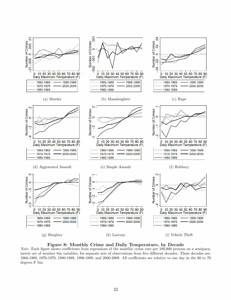
(a) Murder (b) Manslaughter (c) Rape

(d) Aggravated Assault (e) Simple Assault (f) Robbery

(g) Burglary (h) Larceny (i) Vehicle Theft

Figure 8: Monthly Crime and Daily Temperature, by DecadeNote: Each figure shows coefficients from regressions of the monthly crime rate per 100,000 persons on a semipara-metric set of weather bin variables, for separate sets of observations from five different decades. These decades are:1960-1969, 1970-1979, 1980-1989, 1990-1999, and 2000-2009. All coefficients are relative to one day in the 60 to 70degrees F bin.

32

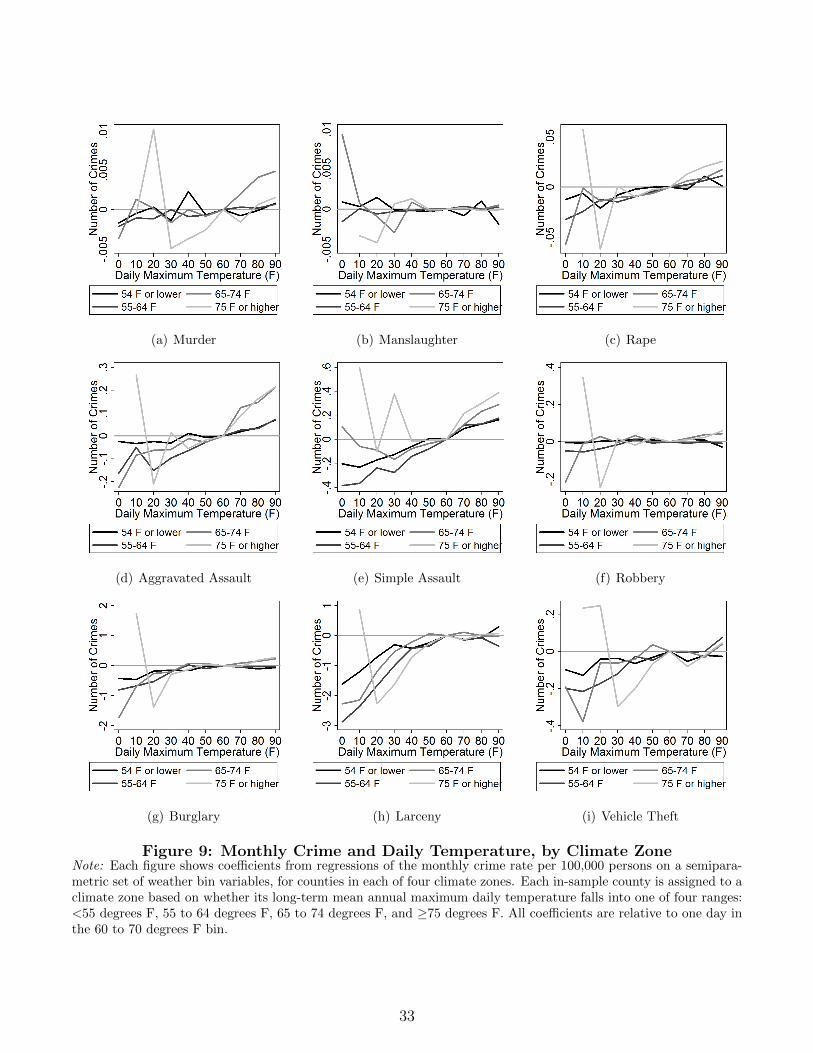
(a) Murder (b) Manslaughter (c) Rape

(d) Aggravated Assault (e) Simple Assault (f) Robbery

(g) Burglary (h) Larceny (i) Vehicle Theft

Figure 9: Monthly Crime and Daily Temperature, by Climate ZoneNote: Each figure shows coefficients from regressions of the monthly crime rate per 100,000 persons on a semipara-metric set of weather bin variables, for counties in each of four climate zones. Each in-sample county is assigned to aclimate zone based on whether its long-term mean annual maximum daily temperature falls into one of four ranges:<55 degrees F, 55 to 64 degrees F, 65 to 74 degrees F, and ≥75 degrees F. All coefficients are relative to one day inthe 60 to 70 degrees F bin.

33

(a) Murder (b) Manslaughter (c) Rape

(d) Aggravated Assault (e) Simple Assault (f) Robbery

(g) Burglary (h) Larceny (i) Vehicle Theft

Figure 10: Monthly Crime and Daily Temperature, by Mean Monthly TemperatureNote: Each figure shows coefficients from a regression of the monthly crime rate per 100,000 persons on a semi-parametric set of weather bin variables, interacted with three county-month temperature category variables. Thesecategorical dummy variables indicate whether the average temperature in each month-by-county, over the periodfrom 1960 to 2009, fell into one of three bins: <45 degrees F, 45 to 69 degrees F, or ≥70 F. All coefficients arerelative to one day in the 60 to 70 degrees F bin.

34

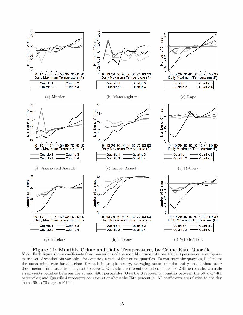
(a) Murder (b) Manslaughter (c) Rape

(d) Aggravated Assault (e) Simple Assault (f) Robbery

(g) Burglary (h) Larceny (i) Vehicle Theft

Figure 11: Monthly Crime and Daily Temperature, by Crime Rate QuartileNote: Each figure shows coefficients from regressions of the monthly crime rate per 100,000 persons on a semipara-metric set of weather bin variables, for counties in each of four crime quartiles. To construct the quartiles, I calculatethe mean crime rate for all crimes for each in-sample county, averaging across months and years. I then orderthese mean crime rates from highest to lowest. Quartile 1 represents counties below the 25th percentile; Quartile2 represents counties between the 25 and 49th percentiles; Quartile 3 represents counties between the 50 and 74thpercentiles; and Quartile 4 represents counties at or above the 75th percentile. All coefficients are relative to one dayin the 60 to 70 degrees F bin.

35

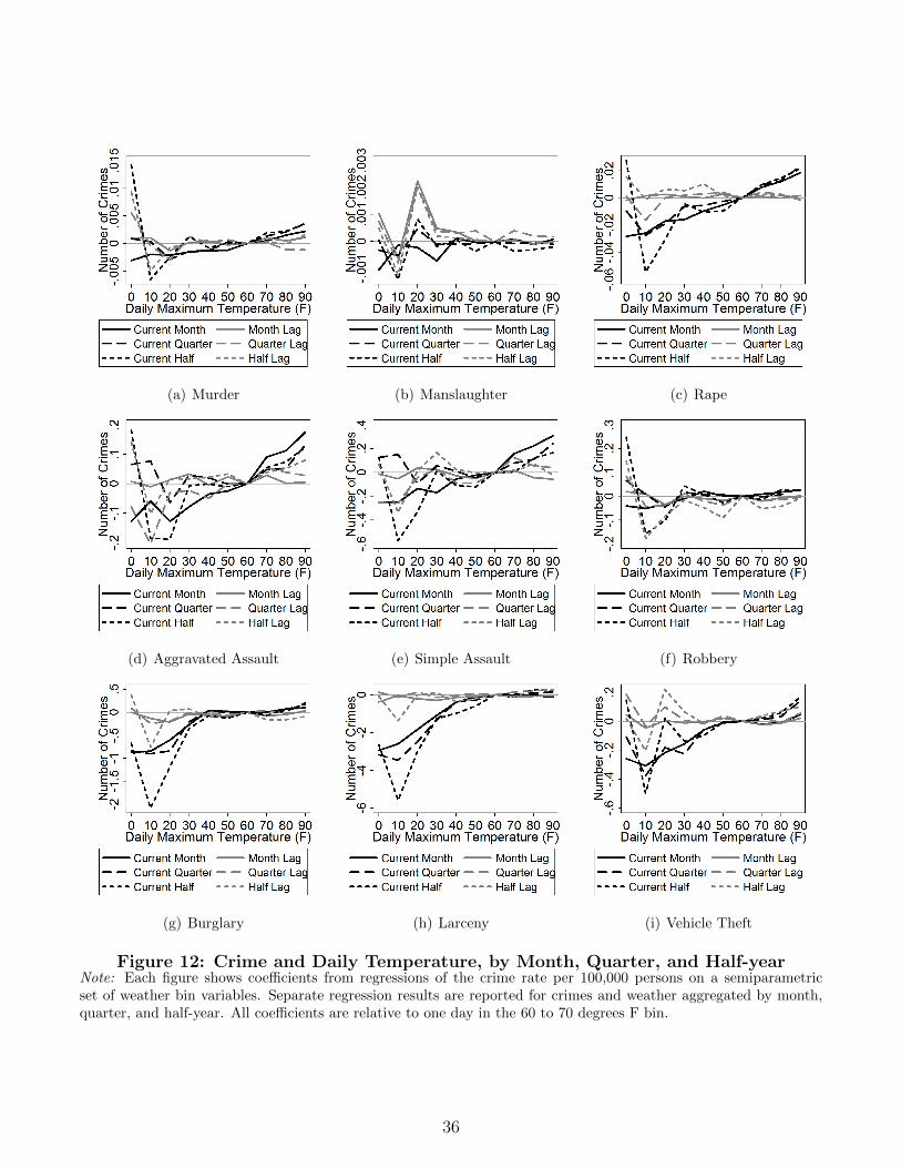
(a) Murder (b) Manslaughter (c) Rape

(d) Aggravated Assault (e) Simple Assault (f) Robbery

(g) Burglary (h) Larceny (i) Vehicle Theft

Figure 12: Crime and Daily Temperature, by Month, Quarter, and Half-yearNote: Each figure shows coefficients from regressions of the crime rate per 100,000 persons on a semiparametricset of weather bin variables. Separate regression results are reported for crimes and weather aggregated by month,quarter, and half-year. All coefficients are relative to one day in the 60 to 70 degrees F bin.

36