UNIVERSITÀ DEGLI STUDI DI CATANIA

FACOLTÀ DI INGEGNERIA

Dipartimento di Ingegneria Elettrica, Elettronica e Informatica

Cristina Ventura

Theoretical and Experimental

Development of a Photovoltaic Power

System for Mobile Robot Applications

Ph.D. Thesis

Electrical Engineering

XXIV Cycle

Supervisor:

Ch.mo Prof. Ing. Tina Giuseppe Marco

December 2011

To my family

Index

i

Index

Abstract iv

Acknowledgement vii

Nomenclature viii

Preface x

CHAPTER I Photovoltaic Systems 1

1.1. Theory ................................................................................................................... 3

1.2. p-n junction ........................................................................................................... 4

1.3. PV cells characteristic ........................................................................................... 5

1.4. Grid connected and Stand-Alone ........................................................................ 11

1.5. Types of PV technology ..................................................................................... 13

1.6. Batteries .............................................................................................................. 15

CHAPTER II Design considerations about a Photovoltaic Power System to Supply a

Mobile Robot 17

2.1. State of the art ..................................................................................................... 19

2.2. The hybrid robot TriBot design .......................................................................... 20

2.2.1. Mechanical design ....................................................................................... 24

2.2.2. Electrical characteristics .............................................................................. 25

2.2.3. Robot Consumption ..................................................................................... 29

2.3. Placement of PV panels analysis ........................................................................ 33

2.4. PV system sizing problem .................................................................................. 36

CHAPTER III A novel MPPT charge regulator for a photovoltaic mobile robot

application 40

3.1. Statement of problem .......................................................................................... 40

3.2. MPPT techniques ................................................................................................ 41

Index

ii

3.2.1. Fractional Open-Circuit Voltage Method .................................................... 44

3.3. MPPT charge regulator ....................................................................................... 45

3.3.1. Fixed reference voltage ............................................................................... 46

3.3.2. Fixed reference voltage with temperature compensation ............................ 47

3.4. Experimental Results .......................................................................................... 48

CHAPTER IV Sub-hourly irradiance models on the plane of array for photovoltaic

energy forecasting applications 55

4.1. Analysis of forecast errors for irradiance on the horizontal plane ...................... 58

4.1.1. Evaluation of the Solar Irradiation Forecasts Errors ................................... 58

4.1.2. Classification of daily solar radiation .......................................................... 59

4.1.3. Neural Network ........................................................................................... 61

4.1.4. Experimental Setup ..................................................................................... 65

4.1.5. Experimental Results ................................................................................... 69

4.2. Clear Sky Radiation Model on Horizontal Surface ............................................ 74

4.2.1. Clear sky direct-beam radiation ................................................................... 74

4.2.2. Clear sky diffuse radiation ........................................................................... 76

4.3. Sub-hourly irradiance models on the plane of array ........................................... 77

4.3.1. Beam and diffuse components of hourly radiation ...................................... 77

4.3.2. Solar Radiation on Inclined Surface ............................................................ 79

4.4. Deriving the temperature profile from the irradiance profile ............................. 94

CHAPTER V Model of a stand-alone photovoltaic system 97

5.1. I-V characteristic generation ............................................................................... 99

5.1.1. The reference parameters ............................................................................ 99

5.1.2. Dependence of the parameters on operating conditions ............................ 102

5.1.3. PV cells temperature and irradiance .......................................................... 104

5.2. Load .................................................................................................................. 106

5.3. Results ............................................................................................................... 106

Summary and Conclusions 113

Index

iii

APPENDIX A Environmental Characteristics 116

6.1. Incident radiation and its components .............................................................. 116

6.2. Solar trajectory .................................................................................................. 117

6.3. Solar Energy ..................................................................................................... 131

Bibliography 138

Abstract

iv

Abstract

The development of mobile robotics structures has recently become an area of great

interest to researchers and industry. These robotics platforms should be, as much as possible,

autonomous and self-sufficient, also from the energetic point of view. In this context, energy

scavengers using small photovoltaic modules have been recently proposed to increase the

autonomy and perform continued operation of embedded systems.

On the basis of this fervent research activity, the primary goal of this work is the

theoretical and experimental development of micro and mini systems for the photovoltaic

production and the energy storage.

Nowadays, the vision of developing perpetual power devices without periodical human

intervention is one of the challenges of embedded systems design. This can be done

harvesting energy efficiently from the environment. In order to account for all the objectives:

lifetime, flexibility, simplicity, cost, up to now, the best compromise appears to be the use of

micro solar power system with rechargeable batteries. The use of this strategy for supplying

systems with limited size and mass, but nevertheless high power requirements, such as a

mobile robot, has been first studied. The system taken as test-bed in the experiment is a bio-

inspired mobile robot, called TriBot.

First of all, a preliminary analysis of the feasibility of a photovoltaic system with batteries

to supply this mobile robot has been done. Considering the different solutions that can be used

to place the PV cells on the robot structure, the different photovoltaic technologies present on

the market with their efficiencies and costs and the power consumption of the robot, the

conclusion is that, using the photovoltaic system here proposed, it is possible to increase the

autonomy of the robot.

Since in the PV system here analyzed the amount of area that can be used to place the PV

cells is very limited and therefore few solar cells can be employed, a very efficient charging

system is an essential requisite. To this aim, a novel photovoltaic charge regulator for mobile

applications, which uses the Fractional Open-Circuit Voltage MPPT method, is proposed. The

purpose of the implemented MPPT algorithm is to optimize the efficiency of the harvesting

process, minimizing the complexity and therefore the power consumption.

Abstract

v

A typical stand-alone photovoltaic system includes a solar array, batteries, regulator and

load. In order to model the whole system and to evaluate its performance, a Simulink model

in Matlab environment has been developed. Meteorological conditions (radiance,

temperature) are essential to estimate the power production of the photovoltaic system. In the

simulator, measured values of the radiation and the temperature have been used. Anyhow, it

will be possible to use predicted values considering the forecast solar radiation and to

calculate the temperature from the solar radiation profile.

In this work, data given us by a weather forecast provider have been used. First of all

these predicted data have been compared with the measured ones, in order to determine their

accuracy, using the normalized Root Mean Square Error (nRMSE) as mean measure. Then, a

method to classify each minute of a day as variable, cloudy, slightly cloudy or clear has been

implemented. In this way it is possible to understand if there is a correlation between the

percentages of the minutes of a specific day that belong to each class and the error done on

that day. Using a neural network, a correlation between these percentages and the error done

in that day has been found.

The knowledge of solar radiation forecasts and therefore the availability of energy for the

batteries and the load is a crucial part for these kinds of autonomous systems whose energetic

consumption is very changeable. The knowledge of the available energy, in fact, should allow

to implement power saving strategies optimizing the activities of the robot.

The weather provider gives us information about the solar radiation on the horizontal

plane. Moreover, the global irradiance on a horizontal surface has been measured in many

meteorological stations around the world, but there are only a few stations that measure this

solar component on inclined surfaces. However, the PV panel exposition is not assumed to be

a control variable due to the fact that the robot can change its posture operating on uneven

terrains. To collect the maximum solar radiation the PV cells have to be oriented toward

south, this is not the case for a moving robots that has to follow the optimal path to carry out

its task. For these reasons, models are required to estimate the solar radiation on the plane of

the PV array starting from the radiation on the horizontal plane. To this aim, in literature there

are a number of models available, but these models require information at the same time on

the global and the direct or diffuse irradiance on a horizontal surface. Consequently, the

variation of the diffuse component with global irradiation has been firstly studied, then the

different methods to calculate the hourly irradiation on the plane of the PV array present in

literature have been analyzed and those which show the best results have been implemented;

Abstract

vi

in particular Perez and Klucher models have been developed. Moreover, a neural network that

allows to evaluate the global solar radiation on the tilted surface directly from the global solar

radiation measured on the horizontal plane, without the need to slit it into the direct and

diffuse components, has been developed.

Once that the solar radiation, measured or forecast, incident on the solar cells used to

recharge the batteries of the robot, at any inclination and orientation the robot will assume; the

power consumption of the robot and the efficiency of the charge regulator are known, all

these information can be used in the Simulink model that, therefore, can become a very

helpful tool to estimate the power production of the photovoltaic system and therefore the

increase of the autonomy of the embedded systems used as load.

Acknowledgement

vii

Acknowledgement

I would first like to thank my supervisor, Professor Ing. Giuseppe Tina, for his

continuous guidance throughout the period of my PhD studies, whose interest, expertise, and

guidance was essential in directing and completing this project.

I would like to express my gratitude to Professor Ing. Paolo Arena, for his support and

constant guide.

For their sympathy and support during these years, many thanks to my colleagues for

their help and support.

I want to remember the inestimable contribution of my family that has always believed in

me, sustaining and encouraging me in all the phases of my personal and professional life.

Finally, an enormous thank to all my friends who offered continual support and needed

distractions.

Nomenclature

viii

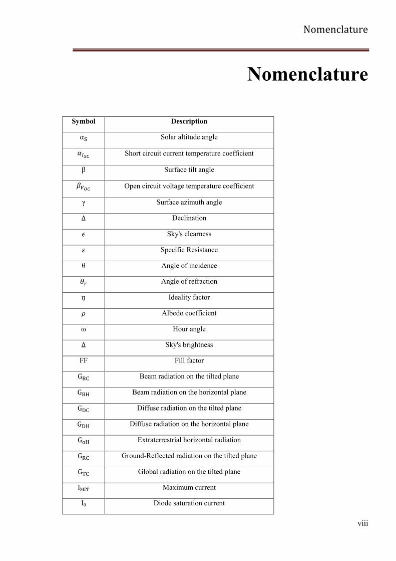
Nomenclature

Symbol Description

Solar altitude angle

Short circuit current temperature coefficient

β Surface tilt angle

Open circuit voltage temperature coefficient

γ Surface azimuth angle

Declination

Sky's clearness

Specific Resistance

θ Angle of incidence

Angle of refraction

Ideality factor

Albedo coefficient

ω Hour angle

Sky's brightness

FF Fill factor

Beam radiation on the tilted plane

Beam radiation on the horizontal plane

Diffuse radiation on the tilted plane

Diffuse radiation on the horizontal plane

Extraterrestrial horizontal radiation

Ground-Reflected radiation on the tilted plane

Global radiation on the tilted plane

IMPP Maximum current

I0 Diode saturation current

Nomenclature

ix

IPH Photo-generated current

ISC Short-circuit current

K Boltzmann‘s gas constant

kt Clearness index

MA Moving Average

MF Moving Function

MSE Mean Square Error

q Electronic charge

RMSE Root Mean Square Error

VMPP Maximum voltage

VOC Open-circuit voltage

Vt Thermal voltage

Preface

x

Preface

In the twenty-first century an emerging theme for the need of more environmentally

benign electric power systems is a critical part of this new thrust. Renewable energy systems

that take advantage of energy sources that won‘t diminish over time and are independent of

fluctuations in price and availability are playing an ever-increasing role in modern power

systems.

Over the past century, fossil fuels provided most of our energy, because these were much

cheaper and more convenient than energy from alternative energy sources, and until recently,

environmental pollution has been of little concern. The main problem is that proven reserves

of oil and gas, at current rates of consumption, would be adequate to meet demand for only

another 41 and 67 years, respectively. The reserves for coal are in a better situation; they

would be adequate for at least the next 230 years. If we try to see the implications of these

limited reserves, we are faced with a situation in which the price of fuels will accelerate as the

reserves decreases. Since the global acknowledgment of the population upon the pollution

generated by coal and oil, the focus is on the renewable energies. Many alternative energy

sources can be used instead of fossil fuels. The decision as to what type of energy source

should be utilized in each case must be made on the basis of economic, environmental, and

safety considerations.

Because of the desirable environmental and safety aspects, it is widely believed that solar

energy should be utilized instead of other alternative energy forms because it can be provided

sustainably without harming the environment. The greatest advantage of solar energy as

compared with other forms of energy is that it is clean and can be supplied without

environmental pollution. Therefore, solar energy technologies can play an important role in

meeting the ultimate goal of replacing fossil fuels to generate inexhaustible, clean and safe

energy.

Up to now, the off-grid PV power generation system is widely used in the portable

applications to provide clear and long energy with a high power density. Nowadays, in fact,

solar energy harvesting has become increasingly important as a way to improve lifetime and

reduce maintenance cost of portable appliances and stand alone power systems. Among

energy harvesting methods, in fact, photovoltaic (PV) sources have the highest energy

Preface

xi

density, they guarantee supply security and sustainable environment; consequently, they

represent, at present, the best way to gather energy from the environment.

In this context, this thesis will focus on the theoretical and experimental development of

micro and mini systems for the photovoltaic production and the energy storage.

In the document, first of all the main characteristics of photovoltaic systems are

introduced, in order to understand how the PV cells convert energy of the solar radiation into

electrical energy.

During the last years, a considerable attention was devoted to the study and development

of robotics structures that can deal with difficult environments to solve complex tasks, such as

outdoor cluttered environment exploration, pipe inspection, mine clearance and others. These

robotic systems can be classified according to their structure, dimensions, maneuverability,

main tasks, and so on. One of the major obstacles in the use of autonomous robots in remote

environments has to do with power supply. Every robot, in fact, requires a power source to

perform all its functions, like navigation, measurements, and manipulations, to name just the

most important. To be autonomous, a robot should perform its duties while maintaining

enough energy to operate. Nowadays, in fact, the vision of developing perpetual power

devices without periodical human intervention is one of the challenges of embedded systems

design. This can be done harvesting energy efficiently from the environment. In this context,

in Chapter II, the use of photovoltaic for supplying systems with limited size and mass, but on

the other hand high power requirements, such as a mobile robot, has been studied. The system

taken as test-bed in the experiment is a bio-inspired mobile robot, called TriBot. Long-term

operation is an important goal of many mobile electronic systems. One may attempt to

achieve this goal in three ways: reduce energy consumption of the system, increase energy

capacity of the battery and replenish battery energy over time. Energy reduction can be done

by improving hardware design and more intelligent power management. Therefore, in order to

built an efficient autonomous power supply system, studies about power consumptions of the

robot have been done. Moreover, some possible structures that will be placed on the robot to

incorporate the PV cells have been analyzed and using AutoCAD, some examples of covering

structures for the robot have been also analyzed.

Unfortunately using photovoltaic systems there are two significant shortcomings: first of

all the conversion efficiency of electric power generation is very low, especially under low

irradiance conditions, moreover the solar panels generate an amount of electric power that

changes continuously with weather conditions. Considering all these problems, the

Preface

xii

optimization of the energy harvesting process under varying light irradiance conditions is

certainly one of the major design challenges for PV systems. Harvested power can be

maximized if the cells and the load are impedance matched in every light irradiance and

temperature conditions. To this aim, in most PV systems a particular technique, namely

Maximum Power Point Tracking (MPPT), is adopted. Therefore, in Chapter III the MPPT

techniques available in literature and a novel MPPT charge regulator for photovoltaic mobile

robot applications are presented.

The stand-alone system presented in this thesis is composed by different parts: PV cells,

batteries, the MPPT charge regulator and load. In order to evaluate the performance of the

whole system, a Simulink model in Matlab environment has been developed. To estimate the

power production of the photovoltaic system, it is needed to know meteorological conditions:

radiance, temperature; these data can be measured or forecast. In the case of forecast values,

in this work, data given us by a weather forecast provider have been used. In Chapter IV, the

accuracy of these predicted data has been evaluated, comparing these with the measured ones.

Then, the method implemented to classify each minute of a day as variable, cloudy, slightly

cloudy or clear has been presented. In this way, it is possible to understand if there is a

correlation between the percentages of the minutes of a specific day that belong to each class

and the error done on that day. The neural network, which allows to find a correlation

between these percentages and the error done in that day, has been described. Forecast solar

radiation allows to know in advance the available energy for the batteries and the load,

therefore power saving strategies for the robot can be implemented. Practically, forecasting

the solar radiation of the day after it is possible to control the actions of the robot basing on

the kind of day; for example, if tomorrow will be clear day, the robot could perform all its

duties without problems, while if tomorrow will be a cloudy day, the robot can preserve its

energy just transmitting data and maintaining a continuous communication of the robot with

other robots and with a base station.

Measured and forecast solar radiations are relative to the horizontal plane. Anyhow, an

autonomous robot can move around the environment and therefore its inclination and

orientation will not always be the same. Accordingly, models are required to estimate the

irradiance on the tilted surface of the PV system from radiation on horizontal ones; these

models are also analyzed.

Preface

xiii

Finally, the model of the PV system developed in Simulink is presented in Chapter V.

This simulator represents a powerful tool to estimate the power production of the photovoltaic

system and therefore the increase of the autonomy of the embedded systems used as load.

All the algorithms and methods have been developed using Matlab environment and

Labview. Matlab has been chosen for the following reasons: it provides many built in

auxiliary functions useful for function optimization, it is completely portable and it is efficient

for numerical computations. While Labview, which was used to acquire measurements from

the external environment, has been chosen because it allows to quickly and easily acquire

real-world signals, to perform analysis to ascertain meaningful data and to communicate or

store results in a variety of ways.

Chapter I

1

CHAPTER I

Photovoltaic Systems

With the increase of the energy demand and the concern of environmental pollution

around the world, photovoltaic power systems are becoming more and more popular.

The sun is regarded as a good source of energy for its consistency and cleanliness, unlike

other kinds of energy such as coal, oil, and derivations of oil that pollute the atmosphere and

the environment. The sun is the only star of our solar system located at its center. The earth

and other planets orbit the sun. Energy from the sun in the form of solar radiation supports

almost all life on earth via photosynthesis and drives the earth‘s climate and weather. Sunlight

is the main source of energy to the surface of the earth that can be harnessed via a variety of

natural and synthetic processes [1]. Basically all the forms of energy in the world are solar in

origin. Oil, coal, natural gas, and wood were originally produced by photosynthetic processes,

followed by complex chemical reactions in which decaying vegetation was subjected to very

high temperatures and pressures over a long period of time. Even the energy of the wind and

tide has a solar origin, since they are caused by differences in temperature in various regions

of the earth.

Most scientists, because of the abundance of sunshine capable of satisfying our energy

needs in the years ahead, emphasize the importance of solar energy [2]. Solar energy is

obviously environmentally advantageous relative to any other renewable energy source, and

the linchpin of any serious sustainable development program. It does not deplete natural

resources, does not cause CO2 or other gaseous emission into air or generates liquid or solid

waste products.

Solar energy is one of the most promising renewable resources that can be used to

produce electric energy through photovoltaic process. A significant advantage of photovoltaic

systems is the use of the abundant and free energy from the sun. Concerning sustainable

development, the main direct or indirectly derived advantages of solar energy are the

following: no emissions of greenhouse (mainly CO2, NOx) or toxic gasses (SO2, particulates),

reclamation of degraded land, reduction of transmission lines from electricity grids, increase

of regional/national energy independence, diversification and security of energy supply,

Chapter I

2

acceleration of rural electrification in developing countries [3]. Moreover, solar energy is a

vital that can make environment friendly energy more flexible, cost effective and

commercially widespread.

Photovoltaic source are widely used today in many applications such as battery charging,

water heating system, satellite power system, and others [4]. Moreover, the off-grid PV power

generation system is widely used in the portable applications to provide clear and long energy

with a high power density.

Photovoltaic modules are solid-state devices that convert sunlight, the most abundant

energy source on the planet, directly into electricity without an intervening heat engine or

rotating equipment [1]. PV equipment has no moving parts and, as a result, requires minimal

maintenance and has a long life. It generates electricity without producing emissions of

greenhouse or any other gases and its operation is virtually silent. PV systems can be built in

virtually any size, ranging be easily added to increase output. PV systems are highly reliable

and in produce a PV panel was more than the energy the panel could produce during its

lifetime. During the last decade, however, due to improvements in the efficiency of the panels

and manufacturing methods, the payback times were reduced to 3–5 years, depending on the

sunshine available at the installation site.

Solar energy is the oldest energy source ever used. The sun was adored by many ancient

civilizations as a powerful god. The first known practical application was in drying for

preserving food [2]. The history of photovoltaics (PVs) began in 1839 when a 19-year-old

French physicist [5], Edmund Becquerel, was able to cause a voltage to appear when he

illuminated a metal electrode in a weak electrolyte solution (Becquerel, 1839). Almost 40

years later, Adams and Day were the first to study the photovoltaic effect in solids (Adams

and Day, 1876). They were able to build cells made of selenium that were 1% to 2% efficient.

Selenium cells were quickly adopted by the emerging photography industry for photometric

light meters; in fact, they are still used for that purpose today. In 1905, Albert Einstein

published four papers in the Annalen der Physik journal; The first one was his explanation of

the photoelectric effect. About the same time, in what would turn out to be a cornerstone of

modern electronics in general, and photovoltaics in particular, a Polish scientist by the name

of Czochralski began to develop a method to grow perfect crystals of silicon. By the 1940s

and 1950s, the Czochralski process began to be used to make the first generation of single-

crystal silicon photovoltaics, and that technique continues to dominate the photovoltaic

industry today.

Chapter I

3

In the 1950s there were several attempts to commercialize PVs, but their cost was

prohibitive. The first practical application of solar cells was in space, where cost was not a

barrier, since no other source of power is available [1]. Research in the 1960s resulted in the

discovery of other photovoltaic materials such as gallium arsenide (GaAs). These could

operate at higher temperatures than silicon but were much more expensive.

Despite their high cost, PV systems are cost effective in many areas that are remote from

utility grids, especially where the supply of power from conventional sources is impractical or

costly. For grid connected distributed systems, the actual value of photovoltaic electricity can

be high because this electricity is produced during periods of peak demand, thereby reducing

the need for costly extra conventional capacity to cover the peak demand. Additionally, PV

electricity is close to the sites where it is consumed, thereby reducing transmission and

distribution losses and thus increasing system reliability.

1.1. Theory

A PV cell consists of two or more thin layers of semiconducting material, most

commonly silicon. When the silicon is exposed to light, electrical charges are generated; and

this can be conducted away by metal contacts as direct current. The electrical output from a

single cell is small, so multiple cells are connected and encapsulated (usually glass covered)

to form a module (also called a panel). The PV panel is the main building block of a PV

system, and any number of panels can be connected together to give the desired electrical

output. This modular structure is a considerable advantage of the PV system, where further

panels can be added to an existing system as required [1].

Therefore, a material or device that is capable of converting the energy contained in

photons of light into an electrical voltage and current is said to be photovoltaic. A photon with

short enough wavelength and high enough energy can cause an electron in a photovoltaic

material to break free of the atom that holds it. If a nearby electric field is provided, those

electrons can be swept toward a metallic contact where they can emerge as an electric current.

The driving force to power photovoltaics comes from the sun, and it is interesting to note that

the surface of the earth receives something like 6000 times as much solar energy as our total

energy demand [5].

Photovoltaics use semiconductor materials to convert sunlight into electricity. The

technology for doing so is very closely related to the solid-state technologies used to make

Chapter I

4

transistors, diodes, and all of the other semiconductor devices that we use so many of these

days [5]. Solar cells are made of semiconductor materials, which are specially treated to form

an electric field, positive on one side (backside) and negative on the other (towards the sun).

The standard silicon (Si) solar cell is based on a semiconductor p-n junction. The contact of n-

doped and p-doped layers forms a p-n junction, where doping is a process of introducing

impurities into a pure semiconductor.

1.2. p-n junction

At present, the most frequent example of solar cell structure is realized with crystalline

silicon (c-Si). A moderately-doped p-type c-Si with an acceptor concentration of 1016

cm3

is

used as the absorber. On the top side of the absorber a thin, less than 1 μm thick, highly-doped

n-type layer is formed as the electron membrane. On the back side of the absorber a highly-

doped p-type serves as the hole membrane. At the interfaces between the c-Si p-type absorber

and the highly-doped n-type and p-type membranes, regions are formed with an internal

electric field [6]. These regions are especially important for solar cells and are known as p-n

junctions. The presence of the internal electric field in the solar cell facilitates the separation

of the photo generated electron-hole pairs. When the charge carriers are not separated from

each other in a relatively short time they will be annihilated in a process that is called

recombination and thus will not contribute to the energy conversion. The easiest way to

separate charge carriers is to place them in an electric field. In the electric field the carriers

having opposite charge are drifted from each other in opposite directions and can reach the

electrodes of the solar cell. The electrodes are the metal contacts that are attached to the

membranes.

The p-n junction fabricated in the same semiconductor material such as c-Si is an

example of the p-n homo-junction. There are also other types of a junction that result in the

formation of the internal electric field in the junction. The p-n junction that is formed by two

chemically different semiconductors is called the p-n hetero-junction. In the p-i-n junctions,

the region of the internal electric field is extended by inserting an intrinsic, i, layer between

the p-type and the n-type layers. The i-layer behaves like a capacitor and it stretches the

electric field formed by the p-n junction across itself. Another type of the junction is a

junction between a metal and a semiconductor, MS junction. The Schottky barrier formed at

the metal-semiconductor interface is a typical example of the MS junction.

Chapter I

5

When a p-n junction is illuminated the additional electron-hole pairs are generated in the

semiconductor. The concentration of minority carriers (electrons in the p-type region and

holes in the n-type region) strongly increases. This increase in the concentration of minority

carriers leads to the flow of the minority carriers across the depletion region into the quasi

neutral regions. Electrons flow from the p-type into the n-type region and holes from the n-

type into the p-type region. The flow of the photo-generated carriers causes the so-called

photo-generation current, IPH.

1.3. PV cells characteristic

A photovoltaic PV generator is mainly an assembly of solar cells, connections, protective

parts, and supports. As was seen already, solar cells are made of semiconductor materials,

usually silicon, and are specially treated to form an electric field with positive on one side

(backside) and negative on the other side, facing the sun.

When solar energy (photons) hits the solar cell, electrons are knocked loose from the

atoms in the semiconductor material, creating electron-hole pairs. If electrical conductors are

then attached to the positive and negative sides, forming an electrical circuit, the electrons are

captured in the form of electric current IPH [3]. From this description, it is obvious to deduce

that during darkness the solar cell is not active and works as a diode, i.e., a p-n junction that

does not produce any current or voltage. If, however, it is connected to an external, large

voltage supply, it generates a current, called the diode or dark current, ID.

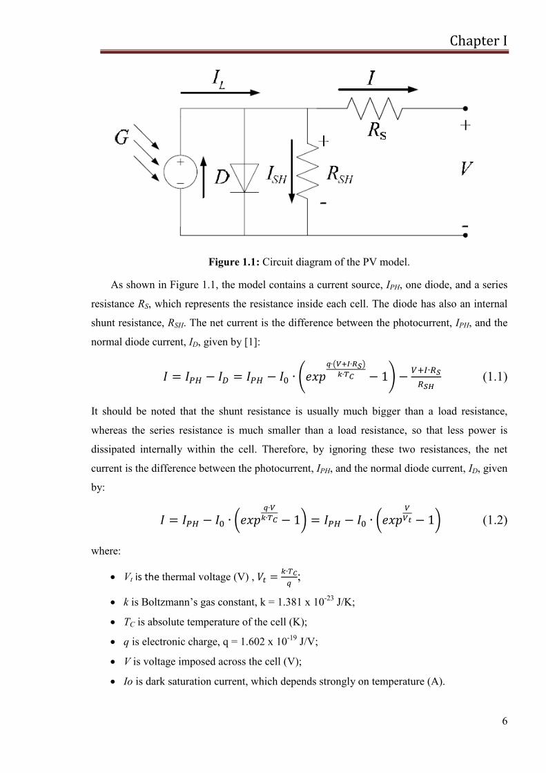
Thus the simplest equivalent circuit of a solar cell is a current source in parallel with a

diode, shown in Figure 1.1. The output of the current source is directly proportional to the

light falling on the cell (photocurrent IPH). A plot of output current against the output voltage

of the solar cell is called the I −V curve when it is under illumination. The I-V characteristic

of the cell is determined by the diode [7].

Chapter I

6

Figure 1.1: Circuit diagram of the PV model.

As shown in Figure 1.1, the model contains a current source, IPH, one diode, and a series

resistance RS, which represents the resistance inside each cell. The diode has also an internal

shunt resistance, RSH. The net current is the difference between the photocurrent, IPH, and the

normal diode current, ID, given by [1]:

(1.1)

It should be noted that the shunt resistance is usually much bigger than a load resistance,

whereas the series resistance is much smaller than a load resistance, so that less power is

dissipated internally within the cell. Therefore, by ignoring these two resistances, the net

current is the difference between the photocurrent, IPH, and the normal diode current, ID, given

by:

(1.2)

where:

Vt is the thermal voltage (V) ,

;

k is Boltzmann‘s gas constant, k = 1.381 x 10-23

J/K;

TC is absolute temperature of the cell (K);

q is electronic charge, q = 1.602 x 10-19

J/V;

V is voltage imposed across the cell (V);

Io is dark saturation current, which depends strongly on temperature (A).

Chapter I

7

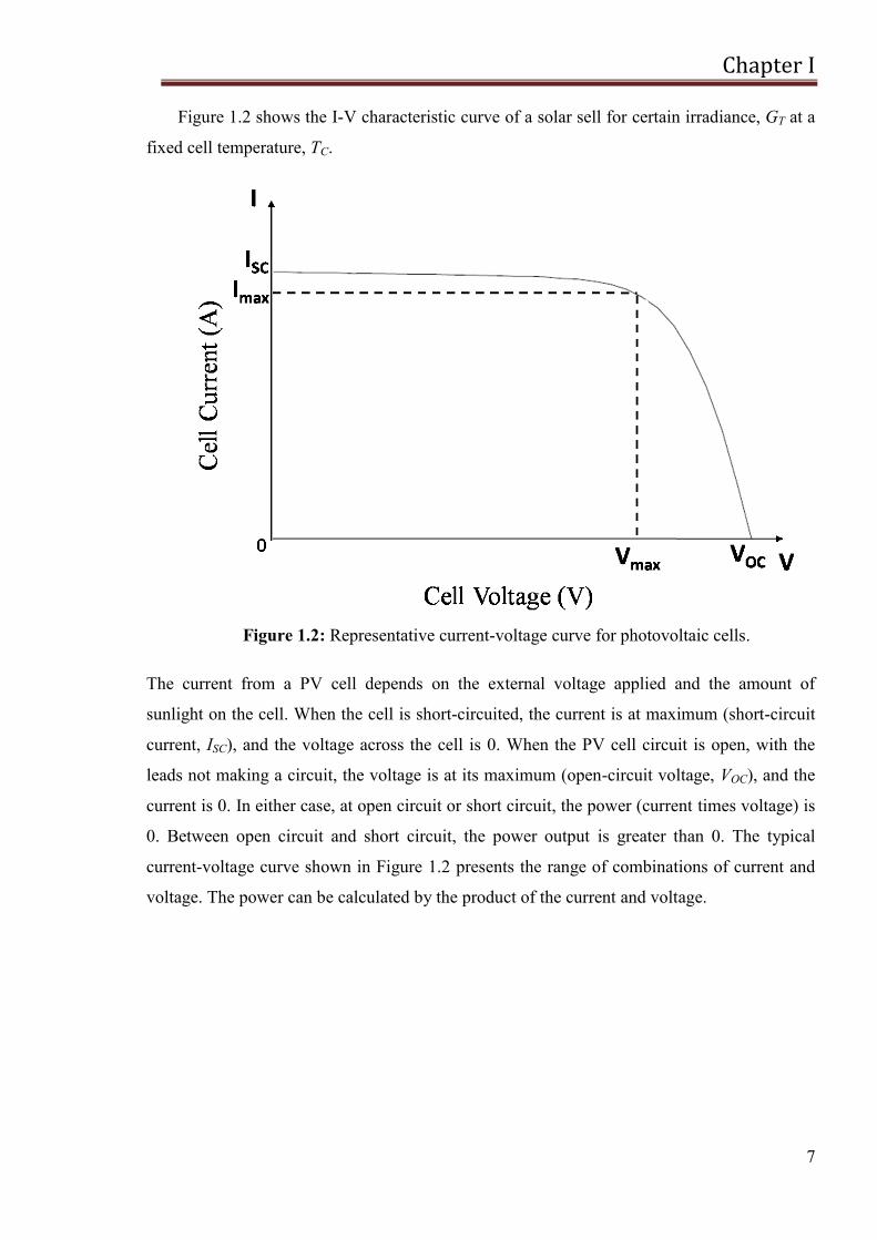
Figure 1.2 shows the I-V characteristic curve of a solar sell for certain irradiance, GT at a

fixed cell temperature, TC.

Figure 1.2: Representative current-voltage curve for photovoltaic cells.

The current from a PV cell depends on the external voltage applied and the amount of

sunlight on the cell. When the cell is short-circuited, the current is at maximum (short-circuit

current, ISC), and the voltage across the cell is 0. When the PV cell circuit is open, with the

leads not making a circuit, the voltage is at its maximum (open-circuit voltage, VOC), and the

current is 0. In either case, at open circuit or short circuit, the power (current times voltage) is

0. Between open circuit and short circuit, the power output is greater than 0. The typical

current-voltage curve shown in Figure 1.2 presents the range of combinations of current and

voltage. The power can be calculated by the product of the current and voltage.

Chapter I

8

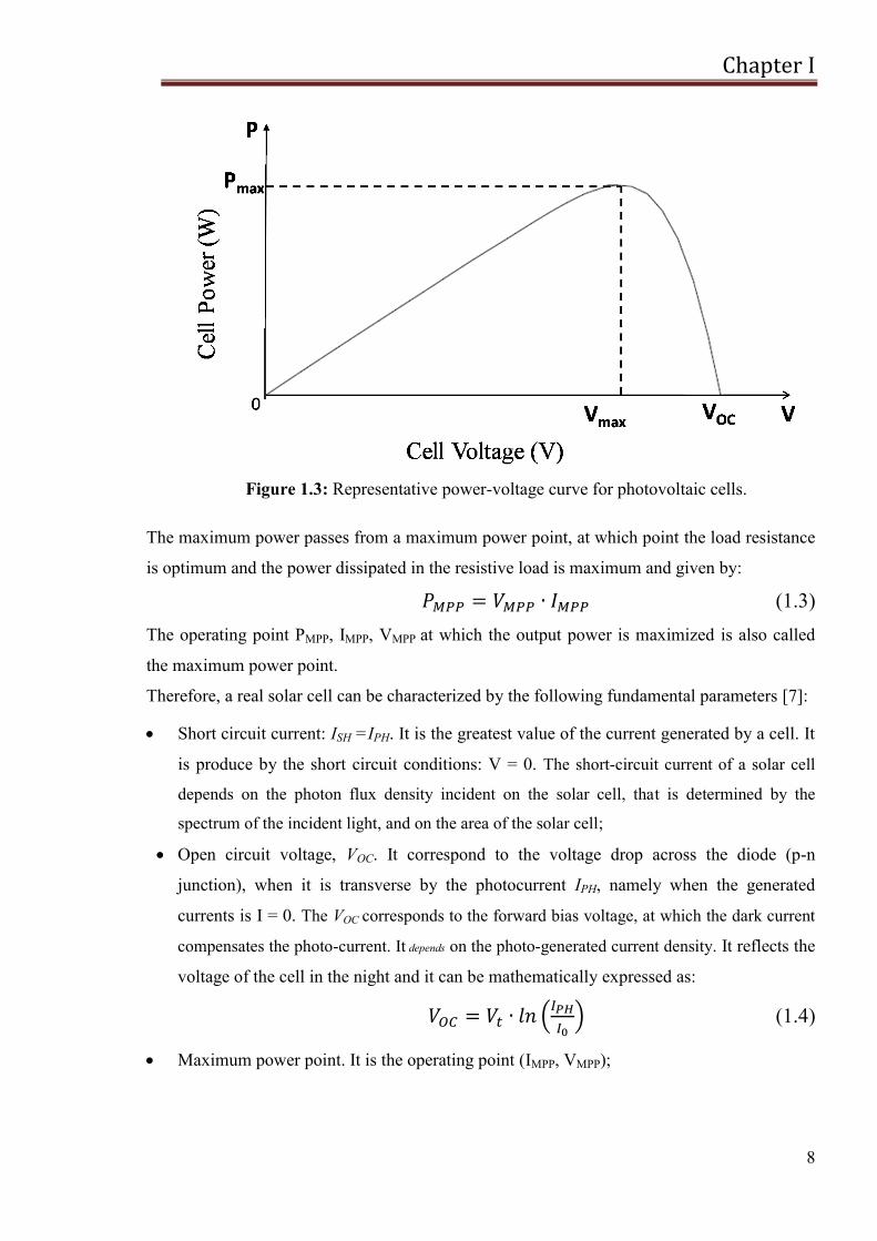
Figure 1.3: Representative power-voltage curve for photovoltaic cells.

The maximum power passes from a maximum power point, at which point the load resistance

is optimum and the power dissipated in the resistive load is maximum and given by:

(1.3)

The operating point PMPP, IMPP, VMPP at which the output power is maximized is also called

the maximum power point.

Therefore, a real solar cell can be characterized by the following fundamental parameters [7]: Short circuit current: ISH =IPH. It is the greatest value of the current generated by a cell. It

is produce by the short circuit conditions: V = 0. The short-circuit current of a solar cell

depends on the photon flux density incident on the solar cell, that is determined by the

spectrum of the incident light, and on the area of the solar cell;

Open circuit voltage, VOC. It correspond to the voltage drop across the diode (p-n

junction), when it is transverse by the photocurrent IPH, namely when the generated

currents is I = 0. The VOC corresponds to the forward bias voltage, at which the dark current

compensates the photo-current. It depends on the photo-generated current density. It reflects the

voltage of the cell in the night and it can be mathematically expressed as:

(1.4)

Maximum power point. It is the operating point (IMPP, VMPP);

Chapter I

9

The conversion efficiency, . It is calculated as the ratio between the generated maximum

power and the incident power. The irradiance value, Pin, of 1000 W/m2

of AM1.5

spectrum has become a standard for measuring the conversion efficiency of solar cells.

(1.5)

Typical external parameters of a crystalline silicon solar cell are: ISC of 35 mA/cm2, VOC

up to 0.65 V and FF in the range 0.75 to 0.80. The conversion efficiency lies in the range

of 17 to 18%.

Fill factor, FF, is the ratio of the maximum power that can be delivered to the load and he

product of ISC and VOC. Given Pmax, it can be calculated such that:

(1.6)

(1.7)

The fill factor is a measure of the real I-V characteristic. Its valued is higher than 0.7 for

good cells. The fill factor diminishes as the cell temperature is increased.

The open circuit voltage increases logarithmically with the ambient irradiation, while the

short circuit current is a linear function of the ambient irradiation. The dominant effect with

increasing cell‘s temperature is the linear decrease of the open circuit voltage, the cell being

thus less efficient. The short circuit current slightly increases with the cell temperature [7].

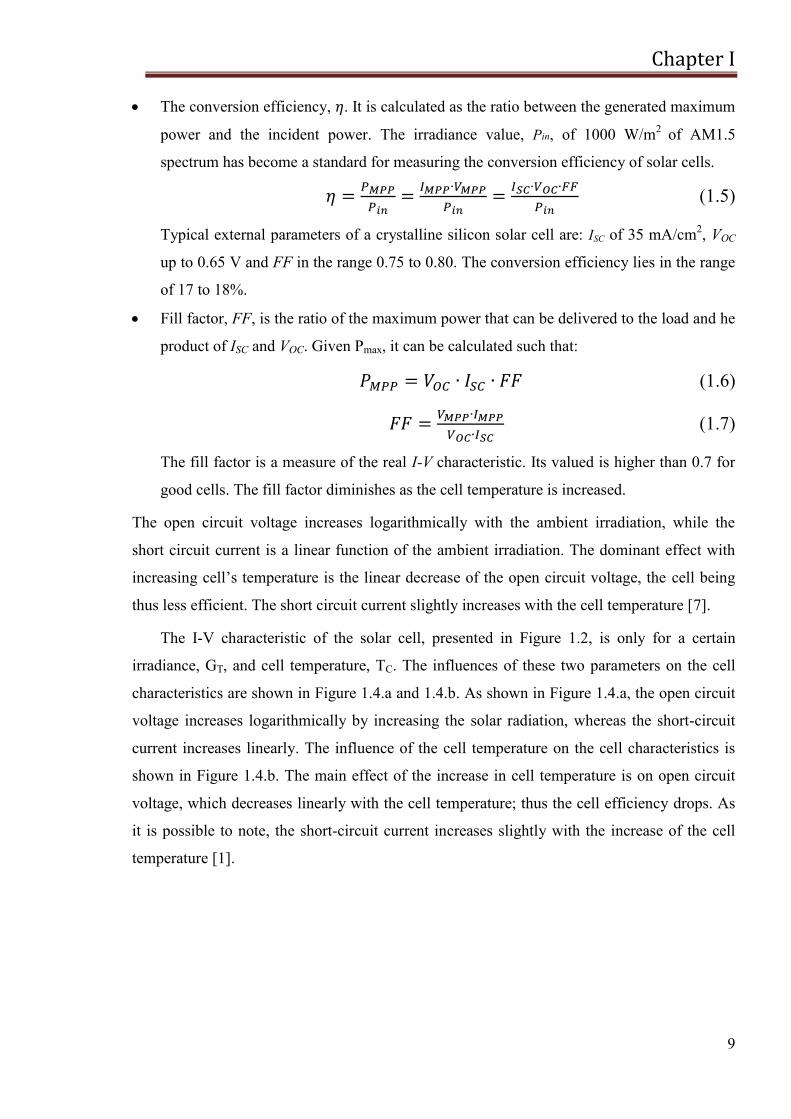
The I-V characteristic of the solar cell, presented in Figure 1.2, is only for a certain

irradiance, GT, and cell temperature, TC. The influences of these two parameters on the cell

characteristics are shown in Figure 1.4.a and 1.4.b. As shown in Figure 1.4.a, the open circuit

voltage increases logarithmically by increasing the solar radiation, whereas the short-circuit

current increases linearly. The influence of the cell temperature on the cell characteristics is

shown in Figure 1.4.b. The main effect of the increase in cell temperature is on open circuit

voltage, which decreases linearly with the cell temperature; thus the cell efficiency drops. As

it is possible to note, the short-circuit current increases slightly with the increase of the cell

temperature [1].

Chapter I

10

(a) (b)

Figure 1.4: Influence of irradiation and cell temperature on PV cell characteristics. (a)

Effect of increased irradiation. (b) Effect of increased cell temperature.

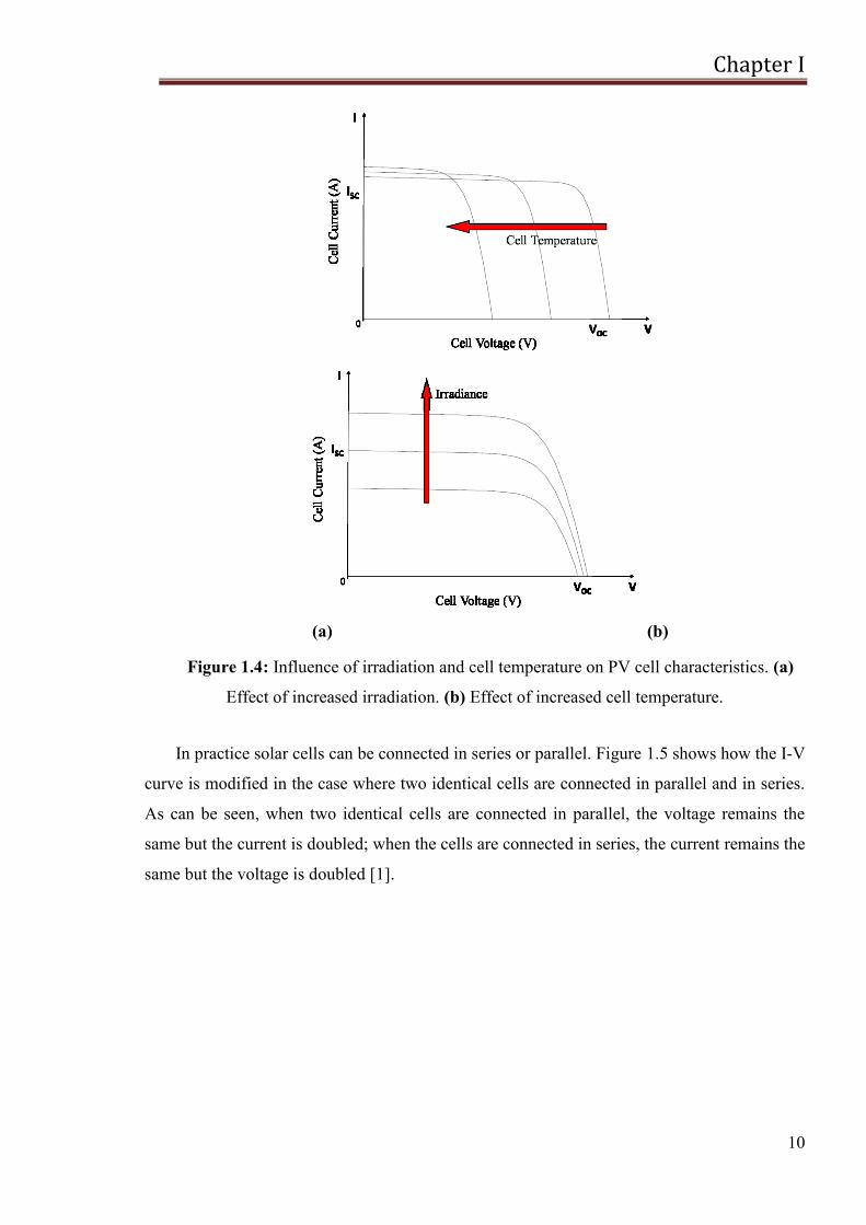
In practice solar cells can be connected in series or parallel. Figure 1.5 shows how the I-V

curve is modified in the case where two identical cells are connected in parallel and in series.

As can be seen, when two identical cells are connected in parallel, the voltage remains the

same but the current is doubled; when the cells are connected in series, the current remains the

same but the voltage is doubled [1].

Chapter I

11

(a) (b)

Figure 1.5: Parallel and series connection of two identical solar cells. (a) Parallel

connection. (b) Series connection.

1.4. Grid connected and Stand-Alone

Photovoltaic applications can be divided into two broad areas [8]:

Grid Connected systems.

- A grid-connected energy system is an independent decentralized power

system that is connected to an electricity transmission and distribution

system (referred to as the electricity grid). They are ideal for locations

close to grid;

- The operational capacity is determined by the supply source. The system

functions only when the supply sources are available;

- Because of the supply driven operation, the system may have to ignore

the local demand during times of unavailability of supply sources;

- The system could be either used to meet the local demand and surplus

can be fed to the grid, or otherwise, the system may exist only to feed the

grid;

- The connectivity to grid enables setting up relatively large-scale systems

and hence they can operate at high plant load factors improving the

economic viability of the operation;

- In a grid-connected power system the grid acts like a battery with an

unlimited storage capacity. So it takes care of seasonal load variations.

Chapter I

12

As a result of which the overall efficiency of a grid-connected system

will be better than the efficiency of a stand-alone system, as there is

virtually no limit to the storage capacity, the generated electricity can

always be stored, and the additional generated electricity need not be

‗‗thrown away‘‘;

- In addition to the initial cost of the system, cost for interface of the

system with grid is incurred;

- For systems operating on renewable sources like biomass, wind and solar

PV, there will be a high pressure on these renewable sources, as the

system usually operates at high scales and need more biomass for its

operation [9, 10, 11].

Stand Alone systems.

- They produce power independently of the utility grid; hence, they are

said to stand-alone. These are more suitable for remotest locations where

the grid cannot penetrate and there is no other source of energy. Stand-

alone systems comprise the majority of photovoltaic installations in

remote regions of the world because they are often the most cost-

effective choice for applications far from the utility grid. Examples are

lighthouses and other remote stations, auxiliary power units for

emergency services or military applications, and manufacturing facilities

using delicate electronics;

- Stand Alone energy systems, the operational capacity is matched to the

demand;

- The needs of the local region assume maximum priority;

- These systems are ideal for remote locations where the system is required

to operate at low plant load factors;

- Operation is mostly seasonal, as the typical stand-alone systems are

usually based on renewable energy technologies like solar PV, which is

not available throughout the year;

- This does not exert pressure on biomass and other renewable energy

sources as it requires fewer resources for small-scale applications;

- These systems are not connected to the utility grid as a result of which

they need batteries for storage of electricity produced during off-peak

Chapter I

13

demand periods, leading to extra battery and storage costs, or else the

excess power generated has to be thrown away.

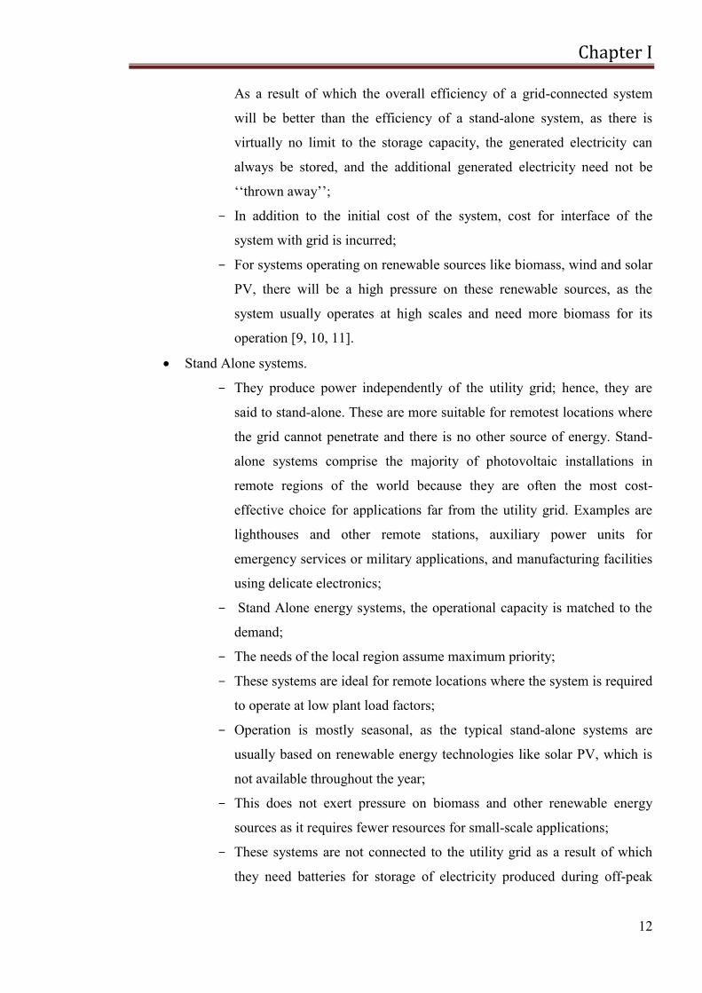
Figure 1.6: Classification of PV Systems [12].

1.5. Types of PV technology

In general, the efficiency of a PV cell to convert incident light into electricity depends on

the used material (technology). Many types of PV cells are available today [1]:

Mono-crystalline silicon cells. These cells are the most common in the PV industry.

They are made from pure mono-crystalline silicon. In these cells, the silicon has a single

continuous crystal lattice structure with almost no defects or impurities. The main

advantage of mono-crystalline cells is their high efficiency, which is typically around

15%. The disadvantage of these cells is that a complicated manufacturing process is

required to produce mono-crystalline silicon, which results in slightly higher costs than

those of other technologies.

Polycrystalline silicon cells. Polycrystalline cells are produced using numerous grains

of mono-crystalline silicon. Compared to single-crystalline silicon, polycrystalline

silicon material is stronger and can be cut into one-third the thickness of single-crystal

material. They are cheaper to produce than mono-crystalline ones because of the

Chapter I

14

simpler manufacturing process required. They are, however, slightly less efficient, with

average efficiencies being around 12%.

Amorphous silicon. Used mostly in consumer electronic products which require lower

power output and cost of production, amorphous silicon is a non-crystalline form of

silicon i.e. its silicon atoms are disordered in structure. Additionally, amorphous silicon

absorbs light more effectively than crystalline silicon, which leads to thinner cells, also

known as a thin film PV technology. The greatest advantage of these cells is that

amorphous silicon can be deposited on a wide range of substrates, both rigid and

flexible. Their disadvantage is the low efficiency, which is on the order of 6%.

Nowadays, the panels made from amorphous silicon solar cells come in a variety of

shapes, such as roof tiles, which can replace normal brick tiles in a solar roof.

Thermo-photovoltaics. These are photovoltaic devices that, instead of sunlight, use the

infrared region of radiation, i.e., thermal radiation. A complete thermo-photovoltaic

(TPV) system includes a fuel, a burner, a radiator, a long wave photon recovery

mechanism, a PV cell, and a waste heat recuperation system [13]. TPV devices convert

radiation using exactly the same principles as photovoltaic devices. The key differences

between PV and TPV conversion are the temperatures of the radiators and the system

geometries.

In addition to the above types, a number of other promising materials, such as cadmium

telluride (CdTe) and copper indium dieseline (CuInSe2), are used today for PV cells. The

main trends today concern the use of polymer and organic solar cells. The attraction of these

technologies is that they potentially offer fast production at low cost in comparison to

crystalline silicon technologies, yet they typically have lower efficiencies (around 4%), and

despite the demonstration of operational lifetimes and dark stabilities under inert conditions

for thousands of hours, they suffer from stability and degradation problems. Organic materials

are attractive, primarily due to the prospect of high-output manufacture using reel-to-reel or

spray deposition. Other attractive features are the possibilities for ultra-thin, flexible devices,

which may be integrated into appliances or building materials, and tuning of color through the

chemical structure [14].

Another type of device investigated is the nano-PV, considered the third generation PV;

the first generation is the crystalline silicon cells, and the second generation is amorphous

silicon thin-film coatings. Instead of the conductive materials and a glass substrate, the nano-

PV technologies rely on coating or mixing ―printable‖ and flexible polymer substrates with

Chapter I

15

electrically conductive nanomaterials. This type of photovoltaics is expected to be

commercially available within the next few years, reducing tremendously the traditionally

high costs of PV cells.

1.6. Batteries

Batteries are required in many PV systems to supply power at night or when the PV

system cannot meet the demand. The selection of battery type and size depends mainly on the

load and availability requirements. When batteries are used, they must be located in an area

without extreme temperatures, and the space where the batteries are located must be

adequately ventilated [1].

The main types of batteries available today include lead-acid, nickel cadmium, nickel

hydride, and lithium. Deep-cycle lead-acid batteries are the most commonly used. These can

be flooded or valve-regulated batteries and are commercially available in a variety of sizes.

Flooded (or wet) batteries require greater maintenance but, with proper care, can last longer,

whereas valve regulated batteries require less maintenance.

The principal requirement of batteries for a PV system is that they must be able to accept

repeated deep charging and discharging without damage. Although PV batteries have an

appearance similar to car batteries, the latter are not designed for repeated deep discharges

and should not be used. For more capacity, batteries can be arranged in parallel.

Batteries are used mainly in stand-alone PV systems to store the electrical energy

produced during the hours when the PV system covers the load completely and there is excess

or when there is sunshine but no load is required. During the night or during periods of low

solar irradiation, the battery can supply the energy to the load. Additionally, batteries are

required in such a system because of the fluctuating nature of the PV system output. Batteries

are classified by their nominal capacity (qmax), which is the number of ampere hours (Ah) that

can be maximally extracted from the battery under predetermined discharge conditions. The

efficiency of a battery is the ratio of the charge extracted (Ah) during discharge divided by the

amount of charge (Ah) needed to restore the initial state of charge. Therefore, the efficiency

depends on the state of charge and the charging and discharging current. The state of charge

(SOC) is the ratio between the present capacity of the battery and the nominal capacity; that

is:

(1.8)

Chapter I

16

As can be understood from the preceding definition and Eq. (1.9), SOC can take values

between 0 and 1. If SOC=1, then the battery is fully charged; and if SOC=0, then the battery

is totally discharged.

Chapter II

17

CHAPTER II

Design considerations about a

Photovoltaic Power System to

Supply a Mobile Robot

The interest in embedded portable systems and wireless sensor networks (WSNs) that

scavenge energy from the environment has been increasing over the last years. Thanks to the

progress in the design of low-power circuits, such devices consume less and less power and

are promising candidates to perform continued operation by the use of renewable energy

sources [15]. The challenges associated with the efficient power management and lifetime of

pervasive embedded systems significantly constraint their functionality and potential

application. In fact, the amount of the energy provided by batteries or other storage devices

still limits their operating lifetime, hence the vision of developing perpetual powered devices

without a necessary periodical maintenance is one of the ultimate goals of embedded systems

design.

In this work, a robotic structure has been chosen as test-bed in the experiments. This

robot is, in fact, a mobile system with limited size and mass, but nonetheless high power

requirements.

A large variety of autonomous robots have been recently developed: these robotic require

a power source to perform all their functions. Robot design is divided into four primary areas:

energy storage, actuation, power and control. It is obvious that there are many relationships

among these phases so as matter of fact they have to be analyzed in parallel to optimize a

robot especially from the energetic point of view.

Different strategies can be used to guarantee energy autonomy to a roving robot: the

introduction of recharge stations in the environment or embed in the robotic structure a power

source generator. The latest solution increases the robot weight and consumptions; therefore,

it is important to explore the added value, in terms of increased autonomy.

Chapter II

18

Environmental energy is an attractive power source for low power wireless sensor

networks. In [16] they present Prometheus, a system that intelligently manages energy

transfer for perpetual operation without human intervention or servicing. Combining positive

attributes of different energy storage elements and leveraging the intelligence of the

microprocessor, they introduce an efficient multi-stage energy transfer system that reduces the

common limitations of single energy storage systems to achieve near perpetual operation.

Experience shows that developing large-scale, long-lived, outdoor sensor networks is

challenging. For this reason, in [17] a new outdoor sensor network deployment that consists

of 557 solar-powered motes, seven gateway nodes, and a root server is described. The test-bed

covers an area of approximately 50,000 square meters and was in continuous operation during

the last four months of 2005. In [18] super-capacitors are used as charge buffers for

alternative power sources. It describes a super-capacitor-operated, solar-powered wireless

sensor node called Everlast. Unlike traditional wireless sensors that store energy in batteries,

Everlast‘s use of super-capacitors enables the system to operate for an estimated lifetime of

20 years without any maintenance. The novelty of this system lies in the feed-forward, PFM

(pulse frequency modulated) converter and open-circuit solar voltage method for maximum

power point tracking, enabling the solar cell to efficiently charge the super-capacitor and

power the node.

Batteries are not a recommended power source for robots that have to work in an isolated

zone, since the power source would limit the lifetime of the system: in this case rechargeable

batteries are a secondary power sources. Therefore, in the context of robot applications,

another primary power source must be used. In order to account for all the objectives:

lifetime, flexibility, simplicity, cost, up to now the best compromise appears to be the use of

micro solar power system with rechargeable batteries.

Here the application of a PV system with rechargeable batteries to power a bio-inspired

robot is discussed. In particular, a power supply solution that utilizes solar cells and a

microcontroller has been chosen to power and control and hybrid robot, named TriBot. One

of the most important characteristic that an autonomous robot should have is to work for an

extended period without human intervention. Therefore, our aim is to design a power system

that makes the robot as much autonomous as possible using solar cells to recharge batteries.

This can allow the robot to have a high exploration capability in open spaces, and to test, on

board, time consuming learning and swarming algorithms without the need to require a

charging phase.

Chapter II

19

2.1. State of the art

Until now, batteries and/or capacitors have been used as power sources. Batteries are

often used to provide power for mobile robots; however, they are heavy to carry and have

limited energy capacity. Therefore power consumption is one of the major issues in robot

design.

Existing studies on energy reduction for robots focus on motion planning to reduce

motion power, for example in [19, 20, 21]. Also in [22] they present an optimal motion

planning of a mobile robot with the objective of minimum energy consumption. The energy

consumption is analyzed in both geometric path planning and smooth trajectory planning. A

global path planner is developed by treating energy efficiency as the central element in the

cost function.

Motion planning for a self-reconfigurable robot involves coordinating the movement and

connectivity of each of its homogeneous modules. Reconfiguration occurs when the shape of

the robot changes from some initial configuration to a target configuration. Finding an

optimal solution to reconfiguration problems involves searching the space of possible robot

configurations. As this space grows exponentially with the number of modules, optimal

planning becomes intractable. On this context, in [23] a global hierarchical motion planning

algorithm for self-reconfigurable modular robotic systems is presented. They impose a

hierarchical structure from input configurations, and utilize a recursive planner that plans at

the top-level of the generated hierarchy by invoking a base planner. However, other

components like sensing, control, communication and computation also consume significant

amounts of power. In [24] two energy-storage techniques are introduced: dynamic power

management and real-time scheduling, which, together with motion planning provide greater

opportunities to increase energy efficiency for mobile robots.

Robots are complex systems that include sensors, actuators, control circuits; for these

reasons the energy request is quite high and the power supply management is an important

aspect for robot design. In [25] a power and propulsion system of an autonomous omni-

directional mobile robot is presented. They proposed a two cascaded cell modules consisting

motor speed control and power flow control modules. The other parts of the robot power

system are dc-dc converters and kicker circuit.

Moreover, there are two strategies for recharging batteries and capacitors: solar panels on

the robot and power stations. Concerning the recharge of batteries, there are two strategies for

Chapter II

20

recharging batteries and capacitors: on board solar panels or off-board power stations. An

example of a colony of hexapod robots, configured with both batteries and capacitors, whose

behavior depends on their power supply status, is presented in [26] and [27]. They explain

how to power and control the hexapod robot Servobot and discuss about a series of legged

robots with high capacitance capacitors for power storage and the configuration of one of

these robots to make practical use of its power storage in a colony recharging system.

Research reported in [27] involves the learning of a control program that allows this robot to

navigate to a charging station. Another example of the use of a power station is presented in

[28]. They discuss about a system for resupplying power to self-contained mobile equipment,

that includes a fixed station having an external power source and consists of a high-frequency

generator and an induction coil as well as a pick-up coil, a current filtering and rectifying

device, a rechargeable battery pack and a microcomputer-controlled tracking system.

Mobile robots often rely on a battery system as their main source of power. These

systems typically produce a single voltage level; however the robot subsystems may require a

set of different voltage levels. In [29] a battery system is used as main power source for a

robot and then the power supply will consist of a combination of switched mode DC power

converters. Experimental results show the converter efficiency and voltage ripple at rated

load. One key design challenge is how to optimize the efficiency of solar energy collection

under non stationary light conditions. In [30], in fact, they propose a scavenger that exploits

miniaturized photovoltaic modules to perform automatic maximum power point tracking at a

minimum energy cost. The system adjusts dynamically to the light intensity variations and its

measured power consumption is less than 1mW.

2.2. The hybrid robot TriBot design

Robotics is a field in continuous evolution. During the last years a considerable attention

was focused on finding new original structures with new mechanics solutions, to face with

complex tasks. Often, solutions already implemented are studied in order to improve them.

Sometime it is very interesting to create hybrid robots, taking advantages from the different

solutions taken into consideration. These were the bases for the design and realization of a

modular hybrid robot named TriBot, where new solutions were studied, trying to find

improvements and to include innovative solutions to add new capabilities to the robot.

Chapter II

21

In last years there is a significant interest in the development of robots capable of

autonomous operations in complex environments. Potential operations for such a robot

include for example mine clearing and terrain mapping. Therefore, critical issues to be solved

to succeed in these operations are: terrestrial mobility, reduced power consumption, efficient

navigation and control strategies, robust communication protocols, and a suitable payload.

When different tasks are taken into consideration, the robot should be able to deal with either

structured (regular) environments or with unstructured environments where the terrain is not

a-priori known.

Mainly, there are two kinds of robots: wheeled and legged, which have different

characteristics. Wheels, in fact, are relatively simple to control, and allow a vehicle to move

quickly over flat terrains [31]. Whereas, a major advantage of legs over wheels is their ability

to gain discontinuous footholds, i.e. they alternate between the stance phase, in which they

contact the substrate, and the swing phase, in which they do not. This approach is suitable on

irregular, discontinuous terrains found in most real-world missions.

Besides, to make a robot as much autonomous as possible, power consumption is of

notable importance. This task is more easily attainable for wheeled robots, because of their

relatively low energy consumption, while, this problem is mostly present in legged robots

that, instead, introduce notable energy consumption. On the other hand, multi-legged robots

are more robust, in fact they can continue moving also with the loss of a single leg. This

characteristic is absent in wheeled vehicles, where a damaged wheel could cause the end of

mobility. Up to now, more than half of the earth‘s landmass is inaccessible to wheeled

vehicles [32]. The same problem is associated to planetary explorations. Moreover, walking

robot performance can be improved taking inspiration from nature, and in particular from

insect, that can run stably over rough terrains at high enough speeds to challenge the ability of

proprioceptive sensing and neural feedback to respond to perturbations within a stride [33].

To summarize, legged robots cannot be view as competing with wheeled machines: it is

rather complementary and is employed in environments otherwise inaccessible.

To deal with complex terrains and the robot has to deal with complex terrains, useful

solutions can be found taking inspiration from nature for mechanical design and locomotion

control, and in particular from the biological principles governing locomotion in insects. An

example of bio-inspired mini robot is MiniHex [34], which is based on the Central Pattern

Generator (CPG) for low level locomotion control. To have both advantages of wheeled and

legged robots it is possible to design a hybrid robot that utilizes a strategy of locomotion

Chapter II

22

which combines the simplicity of wheels with the obstacle clearing advantages of legs.

Examples of wheel-legs robots are Prolero [35], Asguard [36], RHex [37] and Whegs [31].

The peculiar characteristic is the design of Whegs: each leg is in fact realized with a tri-

spoke appendage and is actuated by a single electric motor. This solution tries to fuse together

the powerful capability of wheeled system in terms of speed, payload and easy

maneuverability and also includes the peculiar characteristics of legged systems able to adapt

over rough terrains and to climb obstacles. However, its climbing capabilities are limited if

compared to the classical legs and robots because it cannot change its body posture.

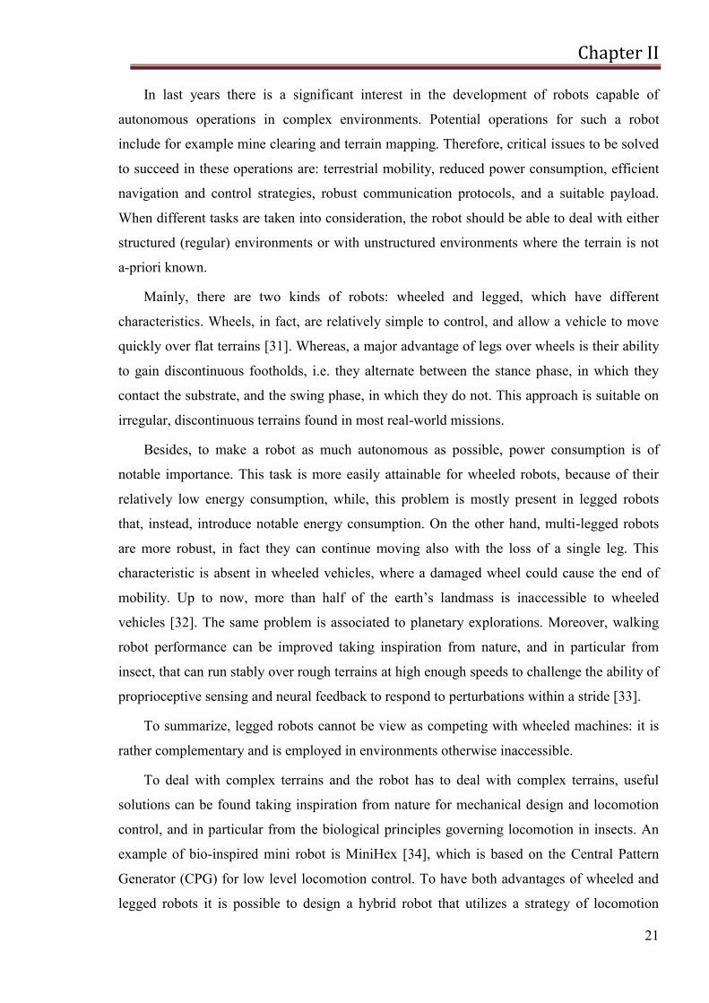
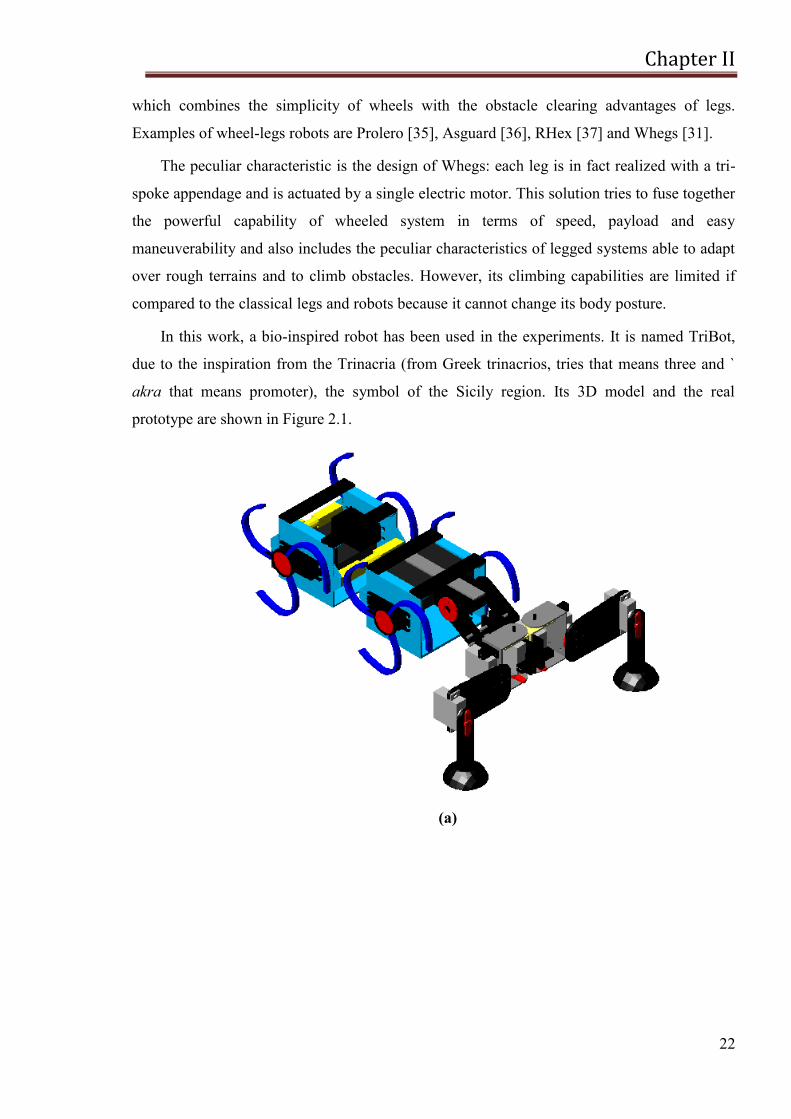
In this work, a bio-inspired robot has been used in the experiments. It is named TriBot,

due to the inspiration from the Trinacria (from Greek trinacrios, tries that means three and `

akra that means promoter), the symbol of the Sicily region. Its 3D model and the real

prototype are shown in Figure 2.1.

(a)

Chapter II

23

(b)

Figure 2.1: Robot TriBot. (a) AutoCAD design; (b) Physic realization.

The design, the realization and the algorithms developed for the locomotion of the robot

taken under consideration were a part of an European project, that is SPARK II "Spatial-

temporal patterns for action-oriented perception in roving robots II: an insect brain

computational model". The purpose of the project was to develop an artificial sensing,

perception and movement that is inspired to the basic principles of the living systems and

based on the concept of "self-organization". The project had a duration of three years, from

February 2008 to February 2011, and inside this wide project, one of the objective was to

study a system able to make the robot autonomous, from the energetic point of view, as much

as possible.

The structure of the robot is constituted by two wheel-legs modules, an optimal solution

for walking in rough terrains and to overcome obstacles. Moreover, a manipulator was added

to improve the capabilities of the system that is able to perform various tasks: environment

manipulation, object grasping, obstacle climbing and others.

In this paragraph, we discuss about the mechanical and electronic elements of the

autonomous mobile robot developed. In particular, the robot design process and the energy

consideration are shown.

Chapter II

24

2.2.1. Mechanical design

The robot has a modular structure; in particular it consists of two wheel-legs modules and

a two-arms manipulator. The two wheel-legs modules are interconnected by a passive joint,

whereas an actuated joint connects these modules with the manipulator that consists of two

legs with three degrees of freedom. To connect the two modules, a passive joint with a spring

have been used. It allows only the pitching movement and facilitates the robot during

climbing, in fact the body flexion easily allows, in a passive way, to adapt the robot posture to

obstacles. Besides, the actuated joint between the two modules and the manipulator allows the

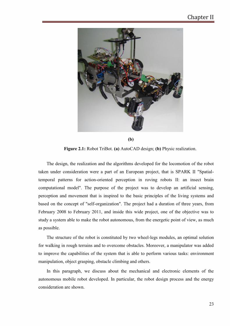
last one to assume two different configurations, therefore it can be useful to improve

locomotion capabilities when it is moved down (i.e. used as legs) (Figure 2.2.a), while when it

is moved up it can make manipulation and grasp objects (i.e. used as arms) (Figure 2.2.b). The

whole mechanical structure is realized in aluminum and plexiglass; both materials have been

selected for their characteristics of cheapness and lightness.

(a) (b)

Figure 2.2: Different robot behaviors. (a) The frontal manipulator can be used for

climbing and (b) for taking objects.

The mechanical peculiar characteristic of this robot is the design of Whegs: each leg is in

fact realized with a tri-spoke appendage and is actuated by a single electric motor. It is a

hybrid solution, the result of a study on the efficiency of a wheel-leg hybrid structure; in this

way the robot can have the advantages of using legs, in fact it can easily overcome obstacles

and face with rough terrains. On the other way, wheel-legs have the shape of wheels;

therefore the robot TriBot is able to have a quite smooth movement in regular terrains and so

to reach high speed.

Chapter II

25

The spokes can be moved in two different directions; if each spoke faces the convex part

toward the motion direction, the movement results to be smoother because the wheel-leg has a

quasi continuous contact with the terrain. While, the other configuration is better in

overcoming obstacles because it increases the grip with the terrain.

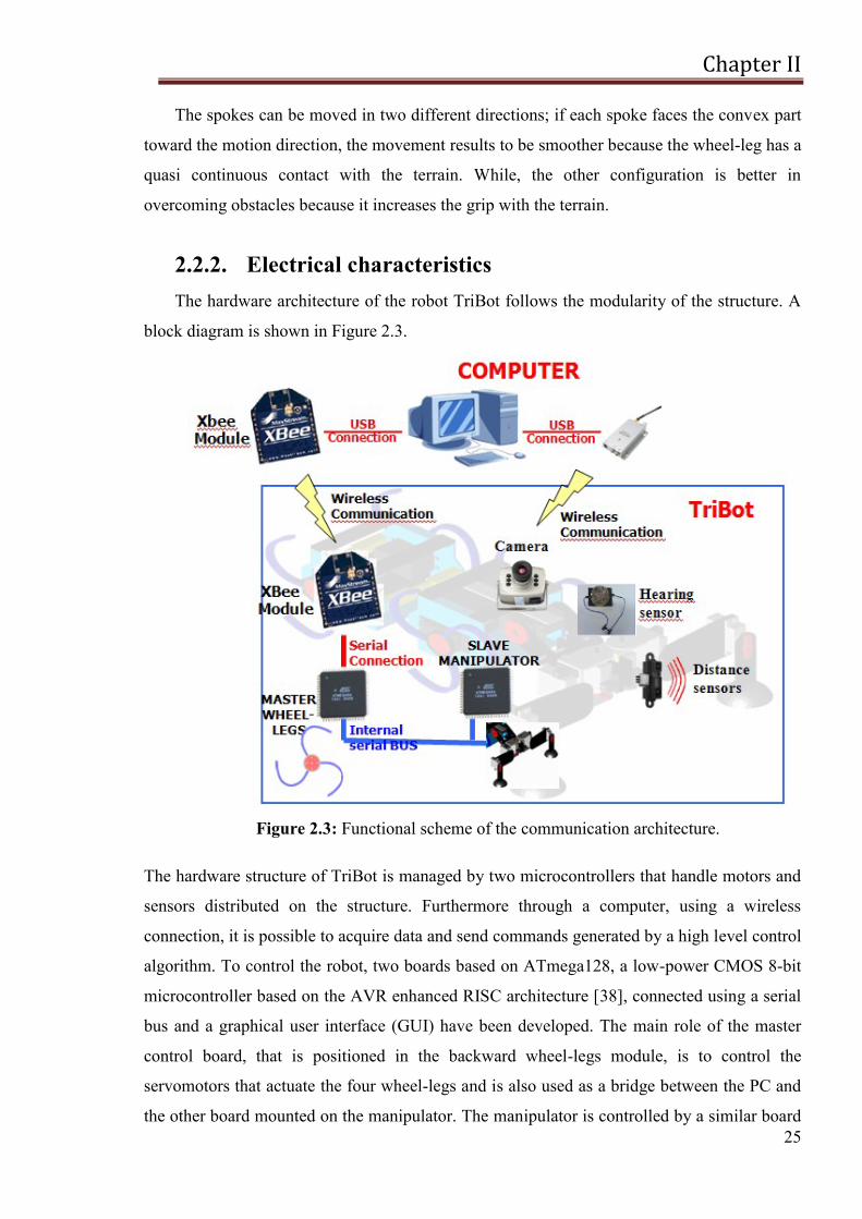
2.2.2. Electrical characteristics

The hardware architecture of the robot TriBot follows the modularity of the structure. A

block diagram is shown in Figure 2.3.

Figure 2.3: Functional scheme of the communication architecture.

The hardware structure of TriBot is managed by two microcontrollers that handle motors and

sensors distributed on the structure. Furthermore through a computer, using a wireless

connection, it is possible to acquire data and send commands generated by a high level control

algorithm. To control the robot, two boards based on ATmega128, a low-power CMOS 8-bit

microcontroller based on the AVR enhanced RISC architecture [38], connected using a serial

bus and a graphical user interface (GUI) have been developed. The main role of the master

control board, that is positioned in the backward wheel-legs module, is to control the

servomotors that actuate the four wheel-legs and is also used as a bridge between the PC and

the other board mounted on the manipulator. The manipulator is controlled by a similar board

Chapter II

26

configured as slave which is used to give the PWM signals to the six servomotors that actuate

the manipulator and to the servomotor that actuates the joint connecting the manipulator with

the rest of the robot. This board has also the important task to read data from the distributed

sensory system embedded in the manipulator. In fact, this robot has been used as test-bed for

the implementation of a correlation-based navigation algorithm, based on an unsupervised

learning paradigm for spiking neural networks, called Spike Timing Dependent Plasticity

(STDP) [39, 40, 41]; to this aim, a sensory system is needed. In particular, on the manipulator,

four distance sensors have been distributed for obstacle detection in order to make the system

able to safely move in unknown environments and a series of micro-switches are used to

detect collisions and to grasp objects. Moreover, the robot is equipped with a compass and a

wireless camera that can be used for landmark identification, following moving objects, and

other higher level tasks.

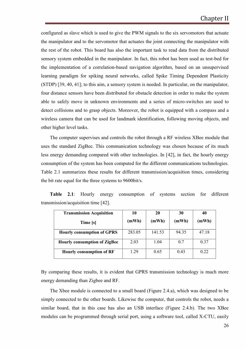
The computer supervises and controls the robot through a RF wireless XBee module that

uses the standard ZigBee. This communication technology was chosen because of its much

less energy demanding compared with other technologies. In [42], in fact, the hourly energy

consumption of the system has been computed for the different communications technologies.

Table 2.1 summarizes these results for different transmission/acquisition times, considering

the bit rate equal for the three systems to 9600bit/s.

Table 2.1: Hourly energy consumption of systems section for different

transmission/acquisition time [42].

Transmission Acquisition

Time [s]

10

(mWh)

20

(mWh)

30

(mWh)

40

(mWh)

Hourly consumption of GPRS 283.05 141.53 94.35 47.18

Hourly consumption of ZigBee 2.03 1.04 0.7 0.37

Hourly consumption of RF 1.29 0.65 0.43 0.22

By comparing these results, it is evident that GPRS transmission technology is much more

energy demanding than Zigbee and RF.

The Xbee module is connected to a small board (Figure 2.4.a), which was designed to be

simply connected to the other boards. Likewise the computer, that controls the robot, needs a

similar board, that in this case has also an USB interface (Figure 2.4.b). The two XBee

modules can be programmed through serial port, using a software tool, called X-CTU, easily

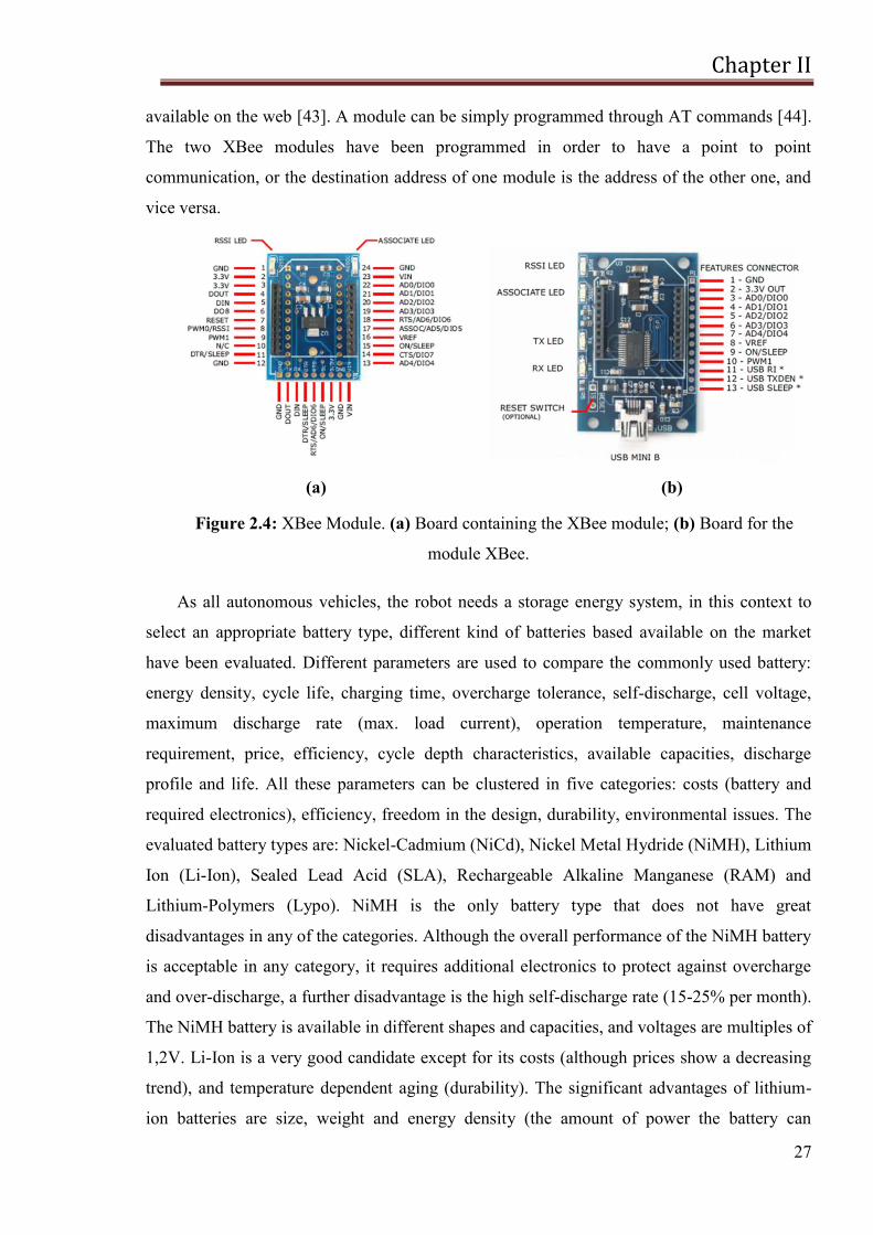
Chapter II

27

available on the web [43]. A module can be simply programmed through AT commands [44].

The two XBee modules have been programmed in order to have a point to point

communication, or the destination address of one module is the address of the other one, and

vice versa.

(a) (b)

Figure 2.4: XBee Module. (a) Board containing the XBee module; (b) Board for the

module XBee.

As all autonomous vehicles, the robot needs a storage energy system, in this context to

select an appropriate battery type, different kind of batteries based available on the market

have been evaluated. Different parameters are used to compare the commonly used battery:

energy density, cycle life, charging time, overcharge tolerance, self-discharge, cell voltage,

maximum discharge rate (max. load current), operation temperature, maintenance

requirement, price, efficiency, cycle depth characteristics, available capacities, discharge

profile and life. All these parameters can be clustered in five categories: costs (battery and

required electronics), efficiency, freedom in the design, durability, environmental issues. The

evaluated battery types are: Nickel-Cadmium (NiCd), Nickel Metal Hydride (NiMH), Lithium

Ion (Li-Ion), Sealed Lead Acid (SLA), Rechargeable Alkaline Manganese (RAM) and

Lithium-Polymers (Lypo). NiMH is the only battery type that does not have great

disadvantages in any of the categories. Although the overall performance of the NiMH battery

is acceptable in any category, it requires additional electronics to protect against overcharge

and over-discharge, a further disadvantage is the high self-discharge rate (15-25% per month).

The NiMH battery is available in different shapes and capacities, and voltages are multiples of

1,2V. Li-Ion is a very good candidate except for its costs (although prices show a decreasing

trend), and temperature dependent aging (durability). The significant advantages of lithium-

ion batteries are size, weight and energy density (the amount of power the battery can

Chapter II

28

provide). Lithium-ion batteries are smaller, lighter and provide more energy than either

nickel-cadmium or nickel-metal-hydride batteries. Additionally, lithium-ion batteries operate

in a wider temperature range and can be recharged before they are fully discharged without

creating a memory problem. An alternative to lithium ion batteries is the lithium polymer cell.

This technology is extremely similar to the lithium ion technology. One advantage to lithium

polymer batteries is that they are more resistant to physical trauma, and moreover they can be

easily shaped to fit many different devices. For these reasons they have been chosen to power

the control boards of the robot.

Furthermore, to obtain the maximum torque and so better performance for the robot,

motors used to actuate the robot need a 6 V power supply. This value has been reached using

NiMH batteries. It is important to take into account that, while in most applications the need

is to have batteries as much light as possible, but at the same time with a high capacity, in this

application the weight of batteries allows to increase the stability of the whole structure. As

matter of fact, at the moment, the robot is equipped with two different battery packs:

10 rechargeable 1.2V, 3000 mAh type Ni-MH AA stylus batteries;

a rechargeable 1345 mAh, 7.4V, Lithium-Polymers battery.

A scheme of the power system of the robot TriBot is shown in Figure 2.5.

Figure 2.5: Flow chart of the TriBot power system.

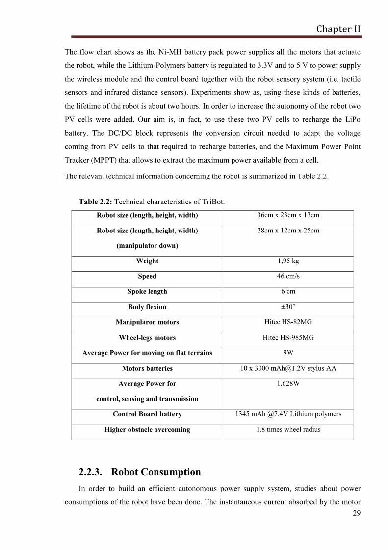
Chapter II

29

The flow chart shows as the Ni-MH battery pack power supplies all the motors that actuate

the robot, while the Lithium-Polymers battery is regulated to 3.3V and to 5 V to power supply

the wireless module and the control board together with the robot sensory system (i.e. tactile

sensors and infrared distance sensors). Experiments show as, using these kinds of batteries,

the lifetime of the robot is about two hours. In order to increase the autonomy of the robot two

PV cells were added. Our aim is, in fact, to use these two PV cells to recharge the LiPo

battery. The DC/DC block represents the conversion circuit needed to adapt the voltage

coming from PV cells to that required to recharge batteries, and the Maximum Power Point

Tracker (MPPT) that allows to extract the maximum power available from a cell.

The relevant technical information concerning the robot is summarized in Table 2.2.

Table 2.2: Technical characteristics of TriBot.

Robot size (length, height, width) 36cm x 23cm x 13cm

Robot size (length, height, width)

(manipulator down)

28cm x 12cm x 25cm

Weight 1,95 kg

Speed 46 cm/s

Spoke length 6 cm

Body flexion ±30°

Manipularor motors Hitec HS-82MG

Wheel-legs motors Hitec HS-985MG

Average Power for moving on flat terrains 9W

Motors batteries 10 x 3000 mAh@1.2V stylus AA

Average Power for

control, sensing and transmission

1.628W

Control Board battery 1345 mAh @7.4V Lithium polymers

Higher obstacle overcoming 1.8 times wheel radius

2.2.3. Robot Consumption

In order to build an efficient autonomous power supply system, studies about power

consumptions of the robot have been done. The instantaneous current absorbed by the motor

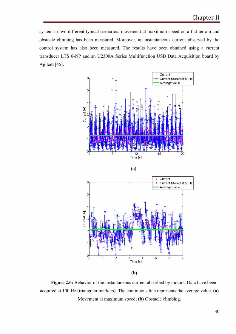
Chapter II

30

system in two different typical scenarios: movement at maximum speed on a flat terrain and

obstacle climbing has been measured. Moreover, an instantaneous current observed by the

control system has also been measured. The results have been obtained using a current

transducer LTS 6-NP and an U2300A Series Multifunction USB Data Acquisition board by

Agilent [45].

(a)

(b)

Figure 2.6: Behavior of the instantaneous current absorbed by motors. Data have been

acquired at 100 Hz (triangular markers). The continuous line represents the average value. (a)

Movement at maximum speed; (b) Obstacle climbing.

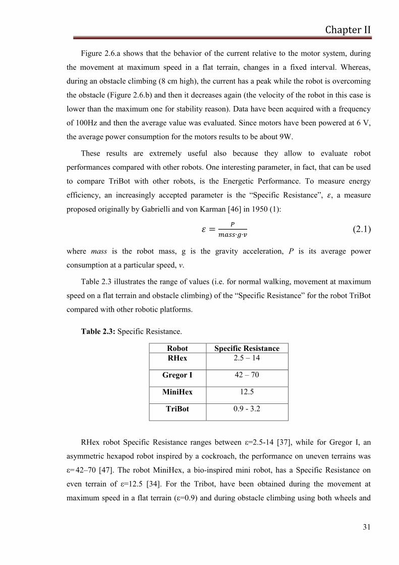
Chapter II

31

Figure 2.6.a shows that the behavior of the current relative to the motor system, during

the movement at maximum speed in a flat terrain, changes in a fixed interval. Whereas,

during an obstacle climbing (8 cm high), the current has a peak while the robot is overcoming

the obstacle (Figure 2.6.b) and then it decreases again (the velocity of the robot in this case is

lower than the maximum one for stability reason). Data have been acquired with a frequency

of 100Hz and then the average value was evaluated. Since motors have been powered at 6 V,

the average power consumption for the motors results to be about 9W.

These results are extremely useful also because they allow to evaluate robot

performances compared with other robots. One interesting parameter, in fact, that can be used

to compare TriBot with other robots, is the Energetic Performance. To measure energy

efficiency, an increasingly accepted parameter is the ―Specific Resistance‖, , a measure

proposed originally by Gabrielli and von Karman [46] in 1950 (1):

(2.1)

where mass is the robot mass, g is the gravity acceleration, P is its average power

consumption at a particular speed, v.

Table 2.3 illustrates the range of values (i.e. for normal walking, movement at maximum

speed on a flat terrain and obstacle climbing) of the ―Specific Resistance‖ for the robot TriBot

compared with other robotic platforms.

Table 2.3: Specific Resistance.

Robot Specific Resistance

RHex 2.5 – 14

Gregor I 42 – 70

MiniHex 12.5

TriBot 0.9 - 3.2

RHex robot Specific Resistance ranges between ε=2.5-14 [37], while for Gregor I, an

asymmetric hexapod robot inspired by a cockroach, the performance on uneven terrains was

ε= 42–70 [47]. The robot MiniHex, a bio-inspired mini robot, has a Specific Resistance on

even terrain of ε=12.5 [34]. For the Tribot, have been obtained during the movement at

maximum speed in a flat terrain (ε=0.9) and during obstacle climbing using both wheels and

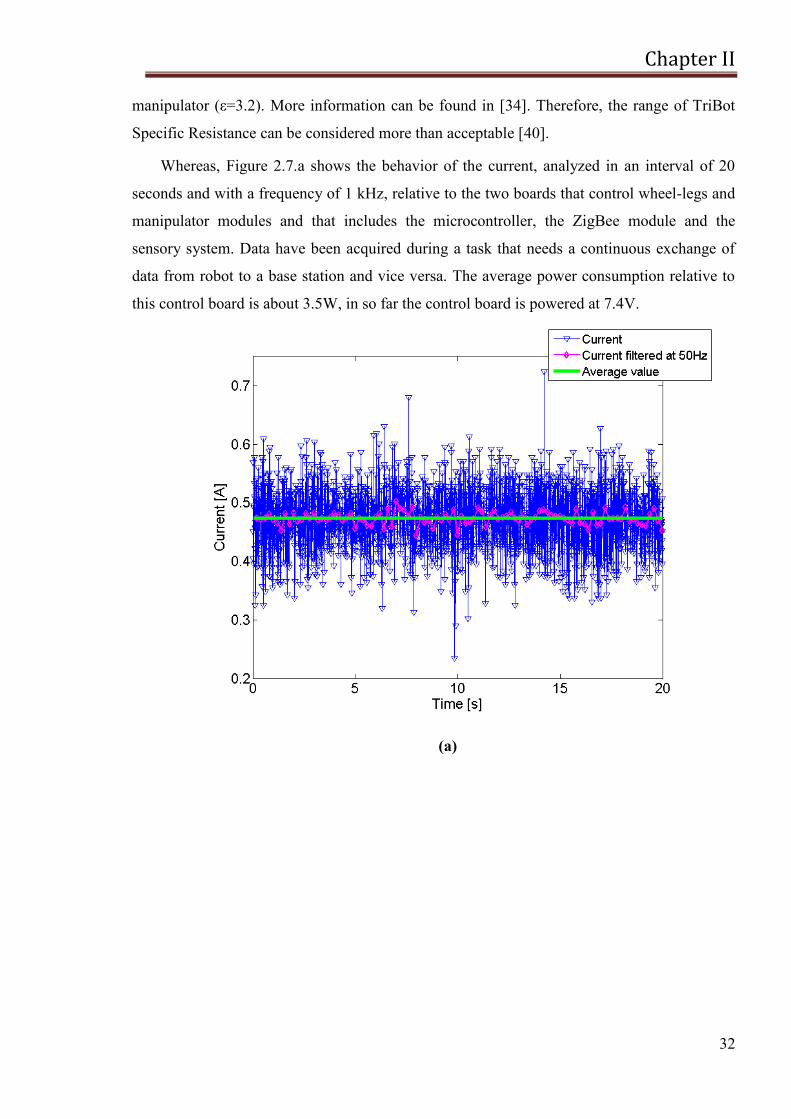
Chapter II

32

manipulator (ε=3.2). More information can be found in [34]. Therefore, the range of TriBot

Specific Resistance can be considered more than acceptable [40].

Whereas, Figure 2.7.a shows the behavior of the current, analyzed in an interval of 20

seconds and with a frequency of 1 kHz, relative to the two boards that control wheel-legs and

manipulator modules and that includes the microcontroller, the ZigBee module and the

sensory system. Data have been acquired during a task that needs a continuous exchange of

data from robot to a base station and vice versa. The average power consumption relative to

this control board is about 3.5W, in so far the control board is powered at 7.4V.

(a)

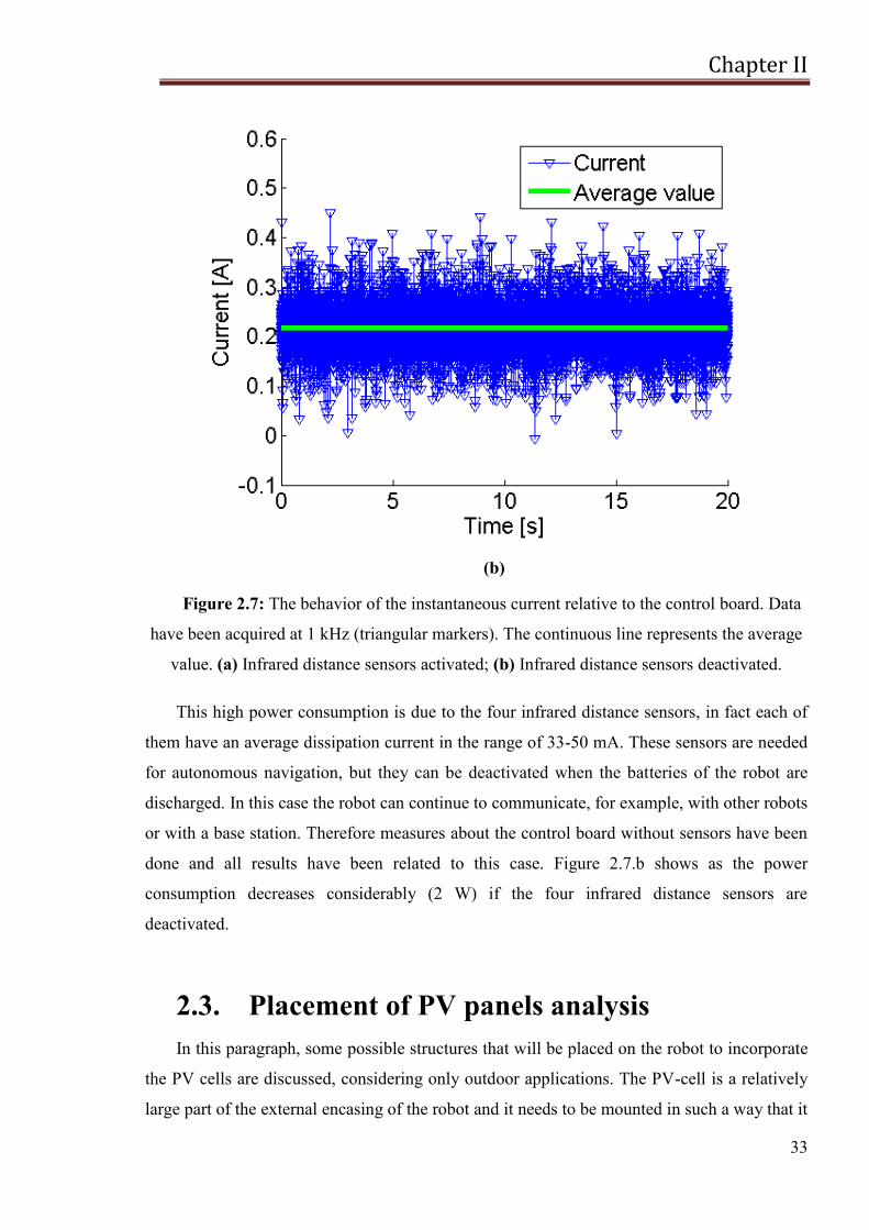
Chapter II

33

(b)

Figure 2.7: The behavior of the instantaneous current relative to the control board. Data

have been acquired at 1 kHz (triangular markers). The continuous line represents the average

value. (a) Infrared distance sensors activated; (b) Infrared distance sensors deactivated.

This high power consumption is due to the four infrared distance sensors, in fact each of

them have an average dissipation current in the range of 33-50 mA. These sensors are needed

for autonomous navigation, but they can be deactivated when the batteries of the robot are

discharged. In this case the robot can continue to communicate, for example, with other robots

or with a base station. Therefore measures about the control board without sensors have been

done and all results have been related to this case. Figure 2.7.b shows as the power

consumption decreases considerably (2 W) if the four infrared distance sensors are

deactivated.

2.3. Placement of PV panels analysis

In this paragraph, some possible structures that will be placed on the robot to incorporate

the PV cells are discussed, considering only outdoor applications. The PV-cell is a relatively

large part of the external encasing of the robot and it needs to be mounted in such a way that it

Chapter II

34

receives as much light as possible. For the studied application, basically three ways of

incorporating the PV-cell exist:

placement in the encasing, under a transparent cover;

placement directly against a transparent cover;

placement outside or as a part of the encasing.

All alternatives include one or more interfaces between media, so that additional

reflection occurs. In order to tackle this problem, the reflection effects need to be understood.

The selected PV cell type should be feasible from both energetic and economic viewpoints.

For an economical evaluation, two different PV technologies can be identified, namely thin

film technology providing encased modules, and crystalline cells (c-Si) with the need for

further module assembling. In PV energy systems c-Si technology is always been

predominant because of its proven reliability and acceptable cost. This kind of cells have

efficiencies are between 12% and 17% and they represent about 90% of the market. Another

technology which has recently advanced in the market is the Thin-Film. Examples of Thin-

Film cells are: amorphous silicon (aSi), copper indium (gallium) diselenide (CIGS) and

cadmium telluride (CdTe). As said in Chapter I, thin-film cells on foils have the advantage to

be bendable and thereby allow higher freedom in solar cell integration into the products

encasing, but show a bad energetic performance. That is, a-Si cells show efficiencies at

determined standard testing conditions around 7% maximum, compared to 13-17% range

efficiencies of commercially produced crystalline cells, with cells up to 20% efficiency

commercially available at relatively low costs. Solar cell efficiency, however, decreases

towards lower radiation, and if the robot will be used in indoor environments, this effect

should be taken into account. Other thin film technologies show rather high efficiencies at

higher light intensities, such as Cu (In,Ga) Se2 (CIGS) and CuInS (CIS) cells, but bad weak

light performance. For example, measured CIS cell efficiency rapidly decreases towards

weaker light intensities with efficiencies below 1% for irradiation below 10W/m2 [48]. If CIS

and/or CIGS cells can prove to have high cell efficiencies also at weaker light intensities, both

technologies are good options for device integrated PV.

Nowadays, the market offers various PV solar panels technologies and, it is clear that, the

shape of these structures depends also on the technology that will be used and, vice versa, the

choice of the technology depends on the energy consumption of the robot and on the available

surface for the installation of the panels. Since the chassis of the robot consists of two

modules with wheel-legs and a manipulator, it is obvious that, to exploit at maximum the

Chapter II

35

available surface of the robot, the PV cells have to be embedded on the two wheel-legs

modules. Each of these two modules is 57mm long, 68mm thick and 54mm tall; therefore, at

most, it is possible to use two 10x10 cm PV cells.

Using AutoCAD, some examples of covering structures have been designed. The

different proposed solutions depend on the technology that will be used. The first possibility

is to use two 10x10cm cells put on the two wheel-legs modules. Using this technology, the

covering structure is rigid and flat; the proposed solution is shown in Figure 2.8.a.

(a)

(b)

Chapter II

36

(c)

Figure 2.8: Proposed covering structure using different PV technologies. (a) Two 10x10

cm2 cells that use the crystalline-silicon (c-Si) technology; (b) Two cells that use the Thin

Film technology; (c) Six 3x10 cm2 cells that use the crystalline-silicon (c-Si) technology.

Figure 2.8.b shows another possible solution. The idea is based on the low profile and

flexibility of thin film cells that allow them to be incorporated with innovative straight or

curved mechanical structures in this case an optimal fit with the robotic structure can be

reached. In this case the covering surface is bigger than the previous one (about 330 cm2), but

it is not an advantageous solution because of the low efficiency of the considered technology.

Finally, using poly-crystalline silicon, it is also possible to obtain 3x10 cm2 cells connected in

series; this would allow to have a greater flexibility in realizing the structure that has to

contain the cells, optimizing the available space. Figure 2.8.c shows another possible shape of

the surface that should contain the PV cells. Solutions (a) and (c) will increase the weight of

the robot of about 5-10 % due to the presence of protective glass layer over the crystalline

silicon cells.

2.4. PV system sizing problem

Unfortunately, there is not a generic procedure for the optimal sizing of an autonomous

energy system that supplies for instance the power needs of the onboard equipment and

instruments of a mobile robot. As a framework for understanding the operation of a solar-

powered micro robot, a generic sizing procedure will be adopted and the various design

choices, difficulties, tradeoffs, and interplay between each component will be investigated.

Chapter II

37

The optimal sizing procedure allows determination of both the optimum power output

required from the Solar Cell Array (SCA), and the optimum capacity of the storage system

which together would supply electric energy required by the robot, especially for control,

sensors and wireless transmission. The objective of the optimization problem is the

maximization of the autonomy of the system. The control variables of the optimization

problem are:

the SCA surface (Ac);

the storage system capacity (Bc).

The optimization process requires the following inputs:

site: latitude, longitude, height, meteorological data;

PV system: PV cells Technology (thin film, mono-crystalline, poly), PV panel

exposition (tilt angle with the horizontal plane and azimuth angle);

battery: type (Lithium, NiCd,etc…), electrical characteristics (Capacity, voltage);

load: components and sensors of the robot, Wireless Communications.

The PV panel exposition is not assumed to be a control variable due to the fact that the robot

can change its posture operating on uneven terrains. To collect the maximum solar radiation

the PV cells have to be oriented toward south, this is not the case for a moving robots that has

to following the optimal path to carry out its task. However, to optimize energy generation, a

navigation strategy that maximizes the efficiency when trying to accomplish the given

mission is envisaged. Finally the robot should be able to find the best stopping position to

recharge the batteries when waiting for new inputs.

During experiments, the energy demand will vary depending on: the wireless

communication technology (and/or the transmission rate), the components and the

management system. The storage system capacity is related with the charge regulator that will

vary depending on the battery type. The hourly energy consumption of the system will be

computed for different configuration and operation schemes of the robot. In [42] a parametric

study on the sizing of PV system with batteries is reported. In this context, it gives an idea of

the ratings of the main components of a standalone PV system: Microcontroller Unit, Sensory

system and Wireless block. The Wireless block is devoted to receive commands from the base

station and to send data storing and monitoring. There are several factors, that affect the

power consumption characteristics of a wireless communication, including the type of

modulation scheme used, data rate, transmit power (determined by the transmission distance),

and the operational duty cycle.

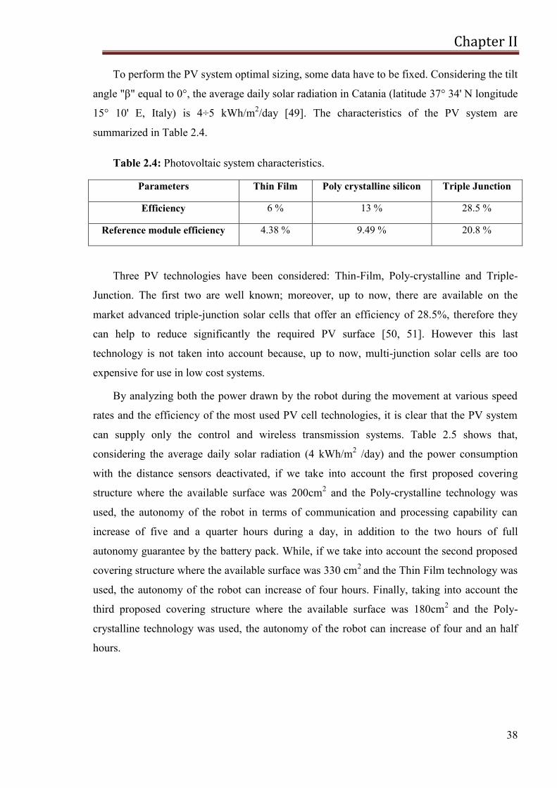
Chapter II

38

To perform the PV system optimal sizing, some data have to be fixed. Considering the tilt

angle "β" equal to 0°, the average daily solar radiation in Catania (latitude 37° 34' N longitude

15° 10' E, Italy) is 4÷5 kWh/m2/day [49]. The characteristics of the PV system are

summarized in Table 2.4.

Table 2.4: Photovoltaic system characteristics.

Parameters Thin Film Poly crystalline silicon Triple Junction

Efficiency 6 % 13 % 28.5 %

Reference module efficiency 4.38 % 9.49 % 20.8 %

Three PV technologies have been considered: Thin-Film, Poly-crystalline and Triple-

Junction. The first two are well known; moreover, up to now, there are available on the

market advanced triple-junction solar cells that offer an efficiency of 28.5%, therefore they

can help to reduce significantly the required PV surface [50, 51]. However this last

technology is not taken into account because, up to now, multi-junction solar cells are too

expensive for use in low cost systems.

By analyzing both the power drawn by the robot during the movement at various speed

rates and the efficiency of the most used PV cell technologies, it is clear that the PV system

can supply only the control and wireless transmission systems. Table 2.5 shows that,

considering the average daily solar radiation (4 kWh/m2 /day) and the power consumption

with the distance sensors deactivated, if we take into account the first proposed covering

structure where the available surface was 200cm2 and the Poly-crystalline technology was

used, the autonomy of the robot in terms of communication and processing capability can

increase of five and a quarter hours during a day, in addition to the two hours of full

autonomy guarantee by the battery pack. While, if we take into account the second proposed

covering structure where the available surface was 330 cm2

and the Thin Film technology was

used, the autonomy of the robot can increase of four hours. Finally, taking into account the

third proposed covering structure where the available surface was 180cm2

and the Poly-

crystalline technology was used, the autonomy of the robot can increase of four and an half

hours.

Chapter II

39

Table 2.5: Evaluation of the autonomy of the robot considering the load power

consumption equal to 2 Wh.

Parameter First solution Second solution Third solution

PV technology Thin Film Poly-crystalline silicon Poly-crystalline silicon

PV cells surface 330cm2 200cm

2 180cm

2

Hours of autonomy for

communication per day

5,25 4 4,2

Therefore, considering these three solutions, the third one, up to now, appears to be the most

appropriate, since it uses the crystalline-silicon technology that has a greater efficiency than

the thin film one and it allows to have more flexibility in the body flexion of the structure.

This solution, in first analysis, considering that the power consumption of the control boards

with sensors deactivated is of about 2W, allows to increase the autonomy of the robot of four

and an half hours [52].

Chapter III

40

CHAPTER III

A novel MPPT charge regulator

for a photovoltaic mobile robot

application

Recently, energy scavengers using small photovoltaic modules have been recently

proposed to increase the autonomy and perform continued operation of embedded systems. In

this context, the aim of this section is to describe the proposed novel smart and simple

photovoltaic charge regulator for a mobile robot.

3.1. Statement of problem

During the last years a considerable attention was devoted to the study and development

of robotics structures that can deal with difficult environments to solve complex tasks. One of

the major obstacles in the use of autonomous robots in remote environments has to do with

power supply. Long-term operation, in fact, is an important goal of many mobile electronic

systems. One may attempt to achieve this goal in three ways: reduce energy consumption of

the system, increase energy capacity of the battery and replenish battery energy over time.

Unfortunately, batteries are limited by both their energy capacities as well as their number of

recharge cycles, even if the system already consumes very low power. As a result, it is

necessary to harvest energy efficiently from the environment.

Up to now solar energy harvesting has become increasingly important as a way to

improve lifetime and reduce maintenance cost of portable appliances and stand alone power

systems: among energy harvesting methods, photovoltaic (PV) sources have the highest

energy density [53], they guarantee supply security and sustainable environment;

Chapter III

41

consequently, they represent, at present, the best way to gather energy efficiently from the

environment.

Therefore, the optimization of the energy harvesting process under varying light

irradiance conditions is certainly one of the major design challenges for PV systems. In fact,

the optimal working voltage of PV cells depends on the specific load, which fixes the output

working voltage. Harvested power can be maximized if the cells and the load are impedance

matched in every light irradiance and temperature condition. To this aim, in most PV systems

a particular technique, namely Maximum Power Point Tracking (MPPT), is adopted.

The aim is to find the operating point (voltage and current) in which the PV panel

operates to obtain the highest possible power. Working in this particular point (MPP) allows

to have several advantages, such as: the minimization of the size of PV modules, the adoption

of smaller energy reservoirs, higher performance or better QoS of the supplied system [15].

MPPT techniques are very common in the world of large-scale solar cells, where a remarkable

amount of energy can be harvested from the environment and where complex models and

circuit simulations of the complex solar power system are employed [54].

However, with the increasing interest in harvesting technologies for portable devices, in

most cases, MPPT techniques have been experimented also on small scales panels, tackling

the development of circuits with power consumption of few mW.

3.2. MPPT techniques

Tracking the maximum power point (MPP) of a photovoltaic (PV) array is usually an

essential part of a PV system. The problem considered by MPPT techniques is to

automatically find the voltage VMPP or current IMPP at which a PV array should operate to

obtain the maximum power output PMPP under a given temperature and irradiance [55]. It is

noted that, under partial shading conditions, in some cases it is possible to have multiple local

maxima, but overall there is still only one true MPP.

Most techniques respond to changes in both irradiance and temperature, but some are

specifically more useful if temperature is approximately constant. Most techniques would

automatically respond to changes in the array due to aging, though some are open-loop and

would require periodic fine tuning. In the last years, a lot of work and research has been done

in the field of MPPT techniques [54, 55, 56] and several methods and algorithms to calculate

Chapter III

42

and track the MPP have been developed. They vary in complexity, sensors required,

convergence speed, cost, range of effectiveness, hardware implementation, popularity and so

on.

The majority of MPPT control strategies depend on characteristics of PV panels in real

time, such as the duty cycle ratio control [57] and using a look-up table. The most used MPPT

techniques are:

Perturbation and Observation (P&O) algorithm: it is based on making perturbation in PV

operation points of a PV panel in order to force the direction of tracking toward an MPP;

Hill-Climbing algorithm: it directly makes a perturbation in a duty cycle of a DC-DC

power converter [58, 59, 60, 61];

Incremental Conductance (IncCond) algorithm: it is implemented by periodically

checking the slope of the P-V curve of a PV panel. If the slope becomes zero or equal to a

defined small value, the perturbation is stopped and the PV panel is forced to work at this

operating point [58, 59, 60, 61, 62];

Fractional Open Circuit Voltage (FOCV): it is based on keeping the ratio between the PV

voltage at the maximum power (VMPP) and the open circuit voltage (VOC) as a constant

value and also in this method the effect of solar irradiance variations is neglected;

Artificial Neural Network method [63];

Fuzzy Logic method [64].

The P&O and IncCond methods are widely used with medium-high power PV modules, since

they allow accurate MPP calculation [55, 65, 66]. However, they require complex control

actions that are often implemented using micro-controllers or DSPs and several

current/voltage sensors. Consequently, the major drawback of these methods is the relatively

high power consumption required to implement the MPPT circuit, which is not manageable in

very low power PV applications. Moreover, these approaches have been effectively used in

stand-alone and grid-connected PV solar energy systems and work well under reasonably

slow and smoothly changing illumination conditions, mainly caused by weather fluctuations.

In [65] and [66] the P&O method is used to make the MPP research more stable and fast

thanks to an auto-adaptive current step. Thanks to an auto-adaptive step and a smart

management, they are able to reach the MPP in a short time and the algorithm stays stable

even with great perturbation of weather conditions.

The design of a hybrid PV system applicable to the public lighting equipments in

apartment buildings is shown in [66]. The system adopts buck-boost converter to regulate the

Chapter III

43

output voltage and also in this case the P&O method is implemented to achieve MPPT. In

[67], a novel stand-alone PV generation system based on a nonlinear MPPT method and

Sinusoidal Pulse-Width Modulation control scheme for single-phase voltage source PWM

inverter has been proposed. In [56] several methods to realize MPPT for large scale PV

system, such as fuzzy logic control, neural network, ripple correlation control (RCC) and so

on are analyzed. Therefore, compact models of PV arrays and their non-linear I-V behavior

already exist for large-scale PV systems [67], after multi-year experience on physics of big

PV modules, circuit simulations and residential solar power systems design. The problem is

that, these methods are complex to be realized; some of them need more sensors and result in

high cost. Therefore, they are not suitable for portable applications. Consequently, similar

models become essential also for small-scale solar harvester design [15].

An MPPT controller suitable for low power PV panels must have low power

consumption, that means low computation complexity and low-power components. In those

applications where few solar cells are employed, in fact, the gain in input energy is not always

higher than the additional losses that are caused by the MPP tracking operation. Therefore, an

MPPT controller for small devices must maximize net power transfer mainly by minimizing

MPPT overhead, while it can afford to sacrifice MPPT accuracy. The energy consumption

and efficiency of the MPP tracker are, therefore, very important design criteria in energy

scavengers for solar-powered mobile applications. In [68] a new low-complexity technique

has been proposed. However, the method has only been tested in a (relatively high-power) 55-

W PV panel and presents a poor tracking efficiency for low power irradiation levels. While, a

new MPPT method suitable for low-power PV panels has been proposed and tested in [69]. In

order to achieve the MPP, the method nulls the difference of the panel average power in two

consecutive time intervals (T1 and T2) within TVcharge.

The main constraint of the solar power system here analyzed, is the limited amount of

area that can be used to place the PV cells on board (about 30 cm2) [52]. This lead to a

maximum available peak power for the adopted PV cells of about 1.4 W. In this context, a

very efficient charging system is mandatory. In order to minimize complexity and therefore

reducing power consumption, while optimizing energy harvesting, FOCV method has been

used.

Chapter III

44

3.2.1. Fractional Open-Circuit Voltage Method

One of the simplest MPPT methods is the Fractional Open-Circuit Voltage (FOCV),

which exploits the nearly linear relationship between the PV panel open-circuit voltage (VOC)

and its voltage at the MPP (VMPP) under varying irradiance and temperature levels, i.e.,

[12, 70, 71, 72]. KFOC is a constant that ranges from 0.71 to 0.78, which

slightly depends on irradiance conditions. Considering KFOC as a constant under different

irradiance conditions leads to small errors in the VMPP evaluation, but strongly simplifies

circuit solutions adopted to implement MPPT. The main drawback of this method is the

dependence of the MPP voltage with temperature. Under the simplified hypothesis that the

series resistance RS is neglectable and under open-circuit conditions (J=0), the relation

between and can be calculated as following:

(3.1)

where

(q is the charge of electron, n is the diode quality factor, k is the

Boltzman constant and TC represents the cell temperature), is the diode saturation current

and represents the photo-generated current. While, when the power is maximum, the

relation is:

(3.2)

Setting Eq. 3.1 equal t<o Eq. 3.2, we have:

(3.3)

If , we obtain:

(3.4)

Under normal condition temperature, Tref = 298.15K, and using amorphous silicon cells, we

have and therefore we obtain:

(3.5)

(3.6)

Chapter III

45

Eq. 3.6 shows as the MPP voltage is doubly dependent from the temperature, implicitly

because depends from the temperature thanks to the heat coefficient and, explicitly,

because also γ depends from temperature. Therefore, in order to get rid of the temperature

dependence of the MPP voltage, a temperature sensor can be exploited.

Using this method the energy used to reach the maximum power is negligible: it is

determined by the current that flows through the voltage divider placed in the input part of the

circuit [73].

3.3. MPPT charge regulator

The goal of this section is to describe the design and implementation of a solar power

system to charge the batteries used to power supply a mobile robot.

Figure 3.1 shows the block diagram of the proposed solar power harvesting system.

Figure 3.1: Block diagram of the solar power system.

The MPPT converter constitutes the heart of the system. It generates the input voltage for

the Li-Po battery charger, which is higher than the typical operation voltage of the PV cells.

Therefore, a high-efficiency switching step-down regulator topology will be adopted. In order

to preserve efficiency, the adopted battery charger is capable of delivering the power

extracted from the PV cells directly to the load in the case the battery is fully charged and in

the case of battery failure.

A power tracking 2A monolithic Multi-Chemistry battery charger for Solar Power

applications, the LT3652EDD [76], has been used. The board is designed to charge 1-cell Li-

Po/Li-Ion batteries using PV cells. Nevertheless, by changing few passive components, the

Chapter III

46

charger accommodates also LiFePO4, Lead-Acid, and NiMH/NiCd chemistries with a

programmable float voltage VBATFLT up to 14.4V. The charger provides a constant-

current/constant-voltage charge characteristic, with maximum charge current externally

programmable up to 2A.

Table 3.1 summarizes its most important characteristics.

Table 3.1: Main characteristics of the charge regulator.

Input voltage 4.5-32 V

Output float voltage 4.2 V

Max load 1 A (Programmable current up to 2 A)

Operating temperature -10°C ÷ 85°C

It contains also two digital open-collector outputs which provide charger status and signal

fault conditions. These binary-coded pins signal battery charging, standby or shutdown

modes, battery temperature faults, and bad battery faults. Moreover, the system comprises a

high performance battery monitor IC (a DS2756 high-precision battery fuel gauge [75]) which

measures the coulometric charge/discharge current (with automatic offset compensation),

battery voltage and temperature. These data, transmitted through the 1-wire HDQ serial

protocol to an intelligent host controller, allow an accurate evaluation of the battery state of

charge (SOC) which, in turn, permits the implementation of power-saving strategies for the

robot. The board also implements the voltage converters supplying the control board of the

robot (3.3V for the processing unit, 5V for the sensors, 9V for the camera). The board contain

provisions for a 6-V converter which can be optionally connected to the board in order to

supply the robot motors.

As already stated the MPPT converter is the most sensitive block of the system and can

be implemented in several different ways. Among the possible solutions, two different

approaches show the best potentialities.

3.3.1. Fixed reference voltage

This solution relies on a step-down converter whose feedback control voltage is

generated by a fixed voltage supply (Figure 3.2). The reference voltage depends upon the

Chapter III

47

particular PV cell type and configuration. However, once the PV cell arrangement is selected,

the optimal reference voltage value can be found by lab measurements.

Figure 3.2: Block Diagram of MPPT converter with fixed reference voltage.

The circuit employs an input voltage regulation loop, which reduces charge current if the

input voltage falls below a programmed level (i.e. the MPP voltage), set with a simple resistor

divider. The MPP voltage can be adjusted in the range 8.5-10.4 V by changing the position of

a trimmer. Since the MPP voltage varies according to the cell temperature, this solution could

show reduced performance if the cells operate under ambient temperature variations greater

than 30°C - 40°C.

3.3.2. Fixed reference voltage with temperature

compensation

In order to get rid of the temperature dependence of the MPP voltage, a temperature

sensor can be exploited. A typical solar panel is comprised of a number of series-connected

cells, each cell being a forward-biased p-n junction [74]. As such, the open-circuit voltage

(VOC) of a solar cell has a temperature coefficient that is similar to a common p-n diode, or

about -2mV/°C. The MPP voltage for solar panel can be approximated as a fixed voltage

below VOC, so the temperature coefficient for the peak power point is similar to that of VOC.

As the temperature characteristic for a typical solar panel MPP voltage is highly linear, a

simple solution for tracking that characteristic can be implemented using temperature sensor

(Figure 3.3). This creates an easily programmable, linear temperature dependent

characteristic. The sensor must be placed under the cells for best results.

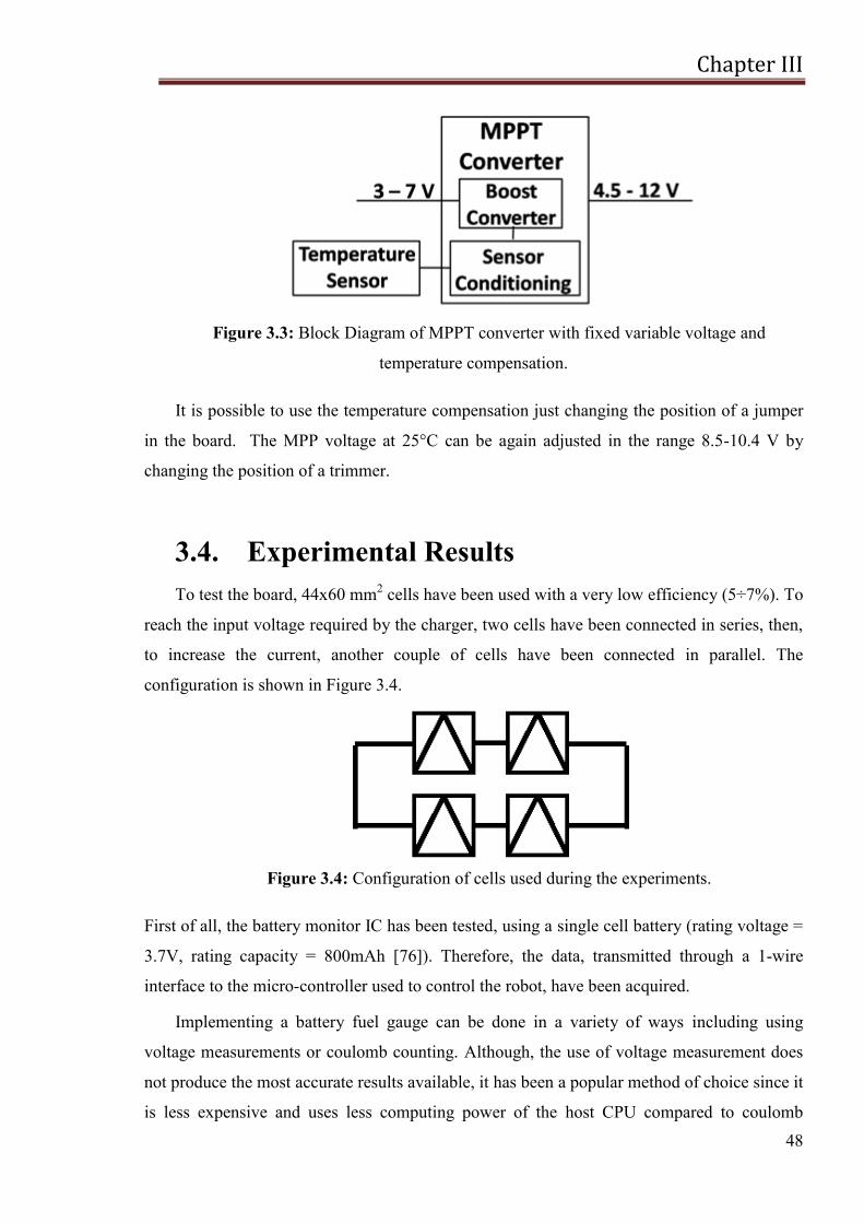
Chapter III

48

Figure 3.3: Block Diagram of MPPT converter with fixed variable voltage and

temperature compensation.

It is possible to use the temperature compensation just changing the position of a jumper

in the board. The MPP voltage at 25°C can be again adjusted in the range 8.5-10.4 V by

changing the position of a trimmer.

3.4. Experimental Results

To test the board, 44x60 mm2 cells have been used with a very low efficiency (5÷7%). To

reach the input voltage required by the charger, two cells have been connected in series, then,

to increase the current, another couple of cells have been connected in parallel. The

configuration is shown in Figure 3.4.

Figure 3.4: Configuration of cells used during the experiments.

First of all, the battery monitor IC has been tested, using a single cell battery (rating voltage =

3.7V, rating capacity = 800mAh [76]). Therefore, the data, transmitted through a 1-wire

interface to the micro-controller used to control the robot, have been acquired.

Implementing a battery fuel gauge can be done in a variety of ways including using

voltage measurements or coulomb counting. Although, the use of voltage measurement does

not produce the most accurate results available, it has been a popular method of choice since it

is less expensive and uses less computing power of the host CPU compared to coulomb

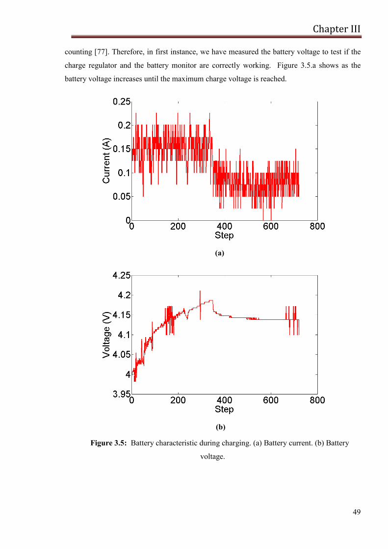
Chapter III

49

counting [77]. Therefore, in first instance, we have measured the battery voltage to test if the

charge regulator and the battery monitor are correctly working. Figure 3.5.a shows as the

battery voltage increases until the maximum charge voltage is reached.

(a)

(b)

Figure 3.5: Battery characteristic during charging. (a) Battery current. (b) Battery

voltage.

Chapter III

50

The LT3652, in fact, can be configured to terminate charging when charge current falls

below 1/10 of the programmed maximum. Once charging is terminated, the LT3652 enters a

low-current standby mode (Figure 3.5.b).

Once verified the correct working of the charge regulator, it is opportune to test how the

use of the MPPT algorithm has really increased the efficiency of the system. To this aim, two

groups of cells connected as before described have been used. The first group has been

connected to an electronic load to study its characteristic and to analyze the power provided

by the PV panel. A LabVIEW interface has been used to acquire data. The other group of

cells has been connected to the charge regulator and then its output has been connected to

another electronic load, regulating, through the LabVIEW interface, the load voltage at a

fixed value. This setup allows to compare the power coming directly from the cells and the

power given to the battery through the charge regulator. All the experiments have been done

in Catania (latitude 37° 34‘ N, longitude 15° 10‘ E, Italy).

In the first experiment, the MPPT converter has been disabled and the load voltage has

been fixed to 3.3V; it has been done on the 9th

November 2010, around at 10 a.m. (the daily

solar radiation in Catania is available [28]). While, the second one has been done using the

FOCV MPPT algorithm (load voltage fixed to 3.3V) on the 23th

November 2010, around at 11

a.m. (the daily solar radiation in Catania is available in [49]). In this case, VMPP has been

calculated by lab measurements and it has been set to 10.23V. Since the FOCV method is

based on the following relation: , the coefficient depends on the value

of VMPP that has been experimentally set through a trimmer and can be modified when it is

considered opportune.

Figure 3.6.a and Figure 3.6.b show the power extracted from the cells, the power

extracted from the charge regulator and the different between them, without using any MPPT

algorithms and using the FOCV MPPT algorithm respectively. While Figure 3.6.c shows as

the efficiency of the implemented charger in the second case is increased of about 8%, thanks

to the use of the MPPT. Therefore, these experiments allow to compare the system when any

MPPT algorithms is used and when the FOCV method is implemented. They demonstrate that

the use of the MPPT technique allows to increase the efficiency of the PV system.

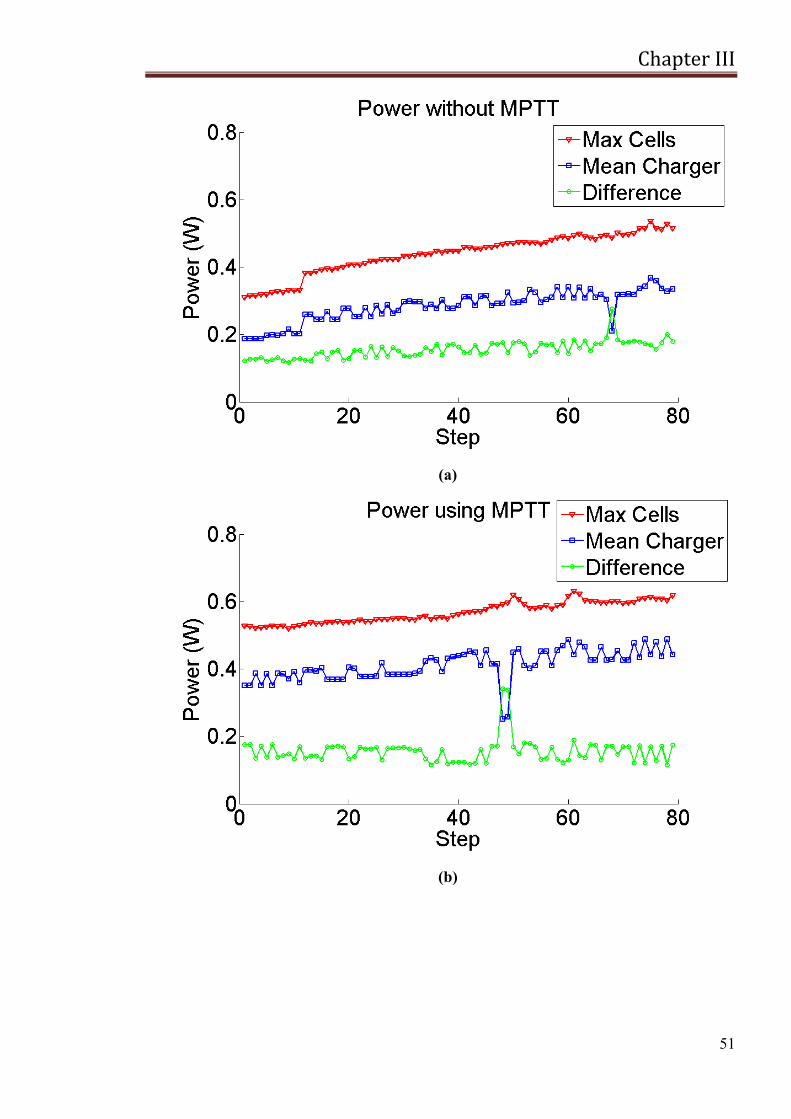
Chapter III

51

(a)

(b)

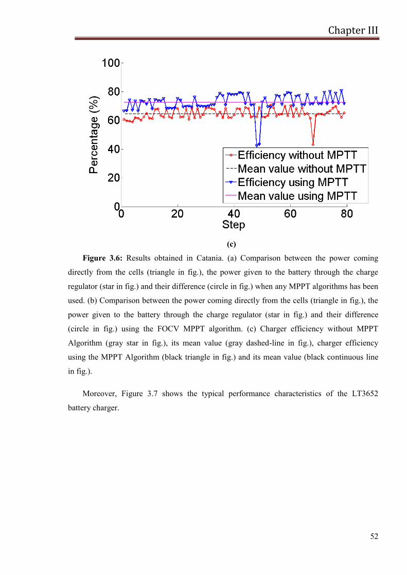
Chapter III

52

(c)

Figure 3.6: Results obtained in Catania. (a) Comparison between the power coming

directly from the cells (triangle in fig.), the power given to the battery through the charge

regulator (star in fig.) and their difference (circle in fig.) when any MPPT algorithms has been

used. (b) Comparison between the power coming directly from the cells (triangle in fig.), the

power given to the battery through the charge regulator (star in fig.) and their difference

(circle in fig.) using the FOCV MPPT algorithm. (c) Charger efficiency without MPPT

Algorithm (gray star in fig.), its mean value (gray dashed-line in fig.), charger efficiency

using the MPPT Algorithm (black triangle in fig.) and its mean value (black continuous line

in fig.).

Moreover, Figure 3.7 shows the typical performance characteristics of the LT3652

battery charger.

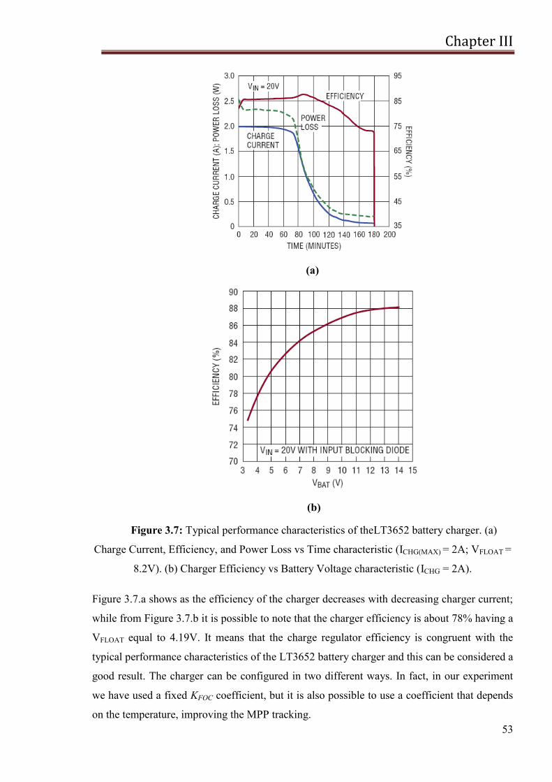
Chapter III

53

(a)

(b)

Figure 3.7: Typical performance characteristics of theLT3652 battery charger. (a)

Charge Current, Efficiency, and Power Loss vs Time characteristic (ICHG(MAX) = 2A; VFLOAT =

8.2V). (b) Charger Efficiency vs Battery Voltage characteristic (ICHG = 2A).

Figure 3.7.a shows as the efficiency of the charger decreases with decreasing charger current;

while from Figure 3.7.b it is possible to note that the charger efficiency is about 78% having a

VFLOAT equal to 4.19V. It means that the charge regulator efficiency is congruent with the

typical performance characteristics of the LT3652 battery charger and this can be considered a

good result. The charger can be configured in two different ways. In fact, in our experiment

we have used a fixed KFOC coefficient, but it is also possible to use a coefficient that depends

on the temperature, improving the MPP tracking.

Chapter III

54

Some qualitative evaluations on the possibility of improving the efficiency of the PV system

changing few components, in order to use batteries with a greater VFLOAT, and at same time

the presence on the market of very efficient PV cells forecast the feasibility to harvest a

greater amount of energy.

Chapter IV

55

CHAPTER IV

Sub-hourly irradiance models on

the plane of array for photovoltaic

energy forecasting applications

Forecasting of solar irradiance is in general significant for planning the operations of

power plants which convert renewable energies into electricity. In particular, the possibility to

predict the solar irradiance (up to 24 h or even more) can became, with reference to the grid

connected photovoltaic plants, fundamental in making power dispatching plans and, with

reference to stand-alone and hybrid systems, also a useful reference for improving the control

algorithms of charge controllers [78]. Daily total solar radiation data, in fact, is considered

such as the most important parameter in the meteorology, solar conversion, and renewable

energy application, particularly for the sizing of stand-alone PV systems. However, these data

are not always available particularly in isolated sites due to the non-availability of the

meteorological stations in these sites and for this reason forecast meteorological data are

needed in such stand-alone systems.

Moreover, over the last years the contribution of power production by PV systems to the

electricity supply has become increasingly relevant. The effect of photovoltaic power

connected to public utilities begins to be noticeable for the overall system and within the next

few years the share of solar produced energy injected on power grids during peak hours will

become noticeable in some areas of the world, especially where legislation encourages the

deployment of increasingly large solar power plants [79]. With this increasing penetration of

photovoltaic (PV) power system into the utility network, the issue caused by the fluctuation

and intermittence of PV power output draws more interest. This power output fluctuation, in

fact, will impact the power system‘s stability. This instability is caused by the dependence of

PV generation on meteorological conditions: irradiance and temperature [80]. If

meteorological conditions can be forecasted with sufficient precision, it will be possible to

Chapter IV

56

estimate the energy a PV system will produce, making photovoltaic a more reliable electricity

source. This forecast information is necessary to improve the assessment of the output of a

photovoltaic system beforehand, allowing a stable integration of such systems in the public

electricity grid. The integration of renewable energy sources, in fact, not only demands

substantial efforts in further development of advanced technologies, but also makes the

availability of precise information on the fluctuating wind and solar resources an

indispensable necessity [81]. Any efficient implementation of wind and solar energy

conversion processes has to account for this behavior in respective operating strategies. A key

issue hereby is the prediction of renewable energy fluxes, typically for time scales from the

sub-hourly range up to two days depending on the given application. Examples are the storage

management in stand-alone photovoltaic or wind energy systems, control systems in

buildings, control of solar thermal power plants and the management of electricity grids with

high penetration rates from renewable sources.

Moreover, forecast information on the expected solar and wind power production is

necessary for the management of electricity grids, for scheduling of conventional power

plants and also for decision making on the energy market [82]. Predictability is, in fact, key to

managing solar and wind power‘s variability and improved accuracy of solar and wind power

prediction has a beneficial effect on the amount of balancing reserves needed, so the accurate

forecasting of solar and wind power is important for their economic integration into the power

system. For an effective application of the power forecast, information on the forecast

accuracy is an important issue. The benefit of prediction intervals for power forecasts is

discussed, e.g., in [83] and [84].

In this work, data given us by a weather forecast provider are used. In this chapter, first of

all these predicted data are compared with the measured ones, in order to determine their

accuracy, using the normalized Root Mean Square Error (nRMSE) as mean measure. Then, a

method to classify each minute of a day as variable, cloudy, slightly cloudy or clear is

implemented. Using a neural network, a correlation between the percentages of the minutes of

a specific day that belong to each class and the error done in that day is found [85].

The weather provider gives us information about the solar radiation on the horizontal

plane. Moreover, the global irradiance on a horizontal surface has been measured in many

meteorological stations around the world, but there are only a few stations that measure this

solar component on inclined surfaces. However, in practice solar collectors (flat plate thermal

or photovoltaic collectors) are tilted, since it allows to maximize the energy production of the

Chapter IV

57

system maximizing the direct irradiance that can be received. Thus, system designers need

data about solar radiation on such titled surfaces; a prerequisite to the design of solar energy

conversion equipment is, in fact, the availability of solar radiation data at the required

location. It would be cost effective when the utility load and solar resource profiles are well

matched. There are great demands for the knowledge of solar radiation data on inclined

surfaces and vertical planes. Solar radiation data are, in fact, very important to architects,

engineers and scientists for energy-efficient building designs the development of active and

passive solar energy applications and climatology and pollution studies.

Estimating solar irradiation incident on inclined surfaces of various orientations is

necessary in order to calculate the building heat gain from the building envelope as well as the

electric power generated by photovoltaics [86], design solar systems and to evaluate their long

term average performance; accordingly, models are required to estimate the irradiance on the

tilted surface of the PV system from radiation on horizontal ones.

There are a number of models available to estimate global irradiance or illuminance on an

inclined surface from the irradiance or illuminance on a horizontal surface, but these models

require information at the same time on the global and the direct or diffuse irradiance or

illuminance on a horizontal surface. Therefore, to calculate the global irradiation on inclined

surfaces from horizontal global irradiation, the first step consists in determining the horizontal

direct or diffuse component. Consequently, in this study the variation of the diffuse

component with global irradiation is firstly studied, then the different methods to calculate the

hourly irradiation on the plane of the PV array present in literature are analyzed and those

which show the best results are implemented. Moreover, a neural network that allows to

evaluate the global solar radiation on the tilted surface directly from the global solar radiation

measured on the horizontal plane, without the need to slit it into the direct and diffuse

components has been developed [87].

While developing the algorithm that allows to classify days thought four values of

percentages: variable, cloudy, slightly cloudy or clear, we have noted that the percentages

calculated on hourly data are less accurate than that ones calculated on data measured every

10 minutes, therefore classification using hourly data appears to be different from the real

one. That happens because, using hourly data, the dynamic of the radiation curve is lost. For

this reason, we have used sub-hourly data instead of hourly solar radiation, and therefore the

radiation on an inclined surface is calculated with a sampling time equal to 10 minutes, on the

Chapter IV

58

contrary of all the models present in literature that have been developed to calculate the

hourly solar radiations.

4.1. Analysis of forecast errors for irradiance on

the horizontal plane

The goal of this section is to analyze the forecast data, verifying their accuracy and to

show the algorithm used to classify days. Moreover the main characteristic of the neural

network here implemented are presented.

4.1.1. Evaluation of the Solar Irradiation Forecasts Errors

To evaluate the errors of the forecasts of solar irradiation, different kinds of errors can be

considered: the root mean absolute error, the mean absolute error, the mean relative variance

and Root Mean Square Error. The root mean square error, RMSE, emphasizes more large

deviation than small ones. The mean absolute error, MAE, provides a linear weighting

between large and small deviations. The mean relative variance, MRV provides a measure

between the error of the forecast of solar irradiation in relation to the variation between the

measured value and the average of all measured values. This measure quantifies the relative

error and is proportional to the standard deviation.

Here, for the evaluation of the accuracy of solar radiation predictions, non-dimensional

forms of the RMSE, the normalized Root Mean Square Error (nRMSE) has been used:

(4.1)

(4.2)

where N is the number of available data, the variable represents the forecast value

of the global irradiance at the t time, while represents the measured one.

The RMSE and the nRMSE are, in fact, frequently used measures of the differences

between values predicted by a model or an estimator and the values actually observed from

the thing being modeled or estimated [79, 88, 89, 90, 91]. The nRMSE has been chosen

because it allows to read in a more understandably way the errors since it is a non-

dimensional parameter (it is expressed in percentage).

Chapter IV

59

4.1.2. Classification of daily solar radiation

The power output and economic viability of a PV plant depends heavily on the solar

irradiance characteristics of its location. Therefore studies that allow to optimize direct normal

irradiance forecasts are required in order to predict the potential power output of a plant. Such

studies are based on daily irradiance records, often with a view to classifying days by cloud

transition patterns and direct radiation variability, because the system response in

concentrating power plants depends on the kind of day. For this reason, a new method based

on Mathematical Morphology techniques for the classification of solar radiation curves, called

MfCM, has been presented in [92]. The main advantage of using this classification is that it

allows to keep the dynamics of the solar radiance curves in the analysis.

Among the standard meteorological variables, solar radiation is the most affected by

cloud cover. In [93] a method for using global and diffuse solar radiation data to classify sky

conditions into several classes is suggested.

In a view to make easier the use of meteorological data as the input of energy systems

simulations, in [94] they proposed a methodology for cloud recognition and sky-condition

classification based on ground-based measurements of broadband solar radiation, and were

able to show that their 4 years of daily data could be clustered into three ―typical‖ sky

condition classes: clear, overcast and cloudy. While, in [95] they deal with the fractal

modeling of daily solar irradiances measured with a sampling time of 10 minutes for one year.

The aim of this modeling was to estimate the fractal index and then to use it to classify the

considered daily irradiances.

Many authors use the clearness index as the starting point for their analysis. This index,

kt, is the mean of the ratio between measured global irradiance and extraterrestrial global

irradiance over a horizontal surface at a specific site, day and time.

(4.3)

where is the global radiation on the horizontal plane and is the extraterrestrial

horizontal radiation (Appendix A).

In [96] classifications considered both, a daily clearness index and a fractal index

introduced by them. Their aim was to estimate the fractal dimensions in order to perform

classification of daily solar irradiances. The results show that these criteria lead to three

classes: clear sky, partially covered sky and overcast sky. A classification of daily

distributions of the clearness index, kt, by estimating a finite mixture of Dirichlet distributions

Chapter IV

60

without assuming any parametric hypothesis on these daily distributions is presented in [97].

Their results reveal four distinct distribution types each representing a different type of day,

namely, ―clear sky days‖, ―intermittent clear sky days‖, ―intermittent cloudy sky days‖ and

―cloudy sky days‖.

In this work, an algorithm used to classify day as variable, cloudy, slightly cloudy or

clear is presented. Practically, each day has been classified according to an algorithm based

on the variation of an index of serenity, k. This index is calculated, each minute, using the

following formula:

(4.4)

where and indicate, respectively, the measured solar radiation value and the

value of the solar radiation calculated using the Liu and Jordan clear sky model (Section 1.2)

[98] in a specific minute of a day.

This index is used to calculate the "Moving Average" (Eq. 4) and "Moving Function"

(Eq. 5), whose values are used in the algorithm to characterize a day:

(4.5)

(4.6)

where NS is the number of the considered minutes used to calculate the moving average.

Studies presented in [99] show how, when averaging data each hour, short periods of

high irradiance are combined with dull periods. However, as the power output of modules

reacts quickly to changes of irradiance while temperature changes are slow modules will often

give higher power than expected at lower module temperatures than calculated from hourly

averages. Since the quick changes of irradiance during a day are essential to correctly classify

a day, in this study we have chosen N=10 if data are calculated each minute, while N=3 if

data are calculated every 10 minutes and for hourly data.

The value of k and MF are used to characterize the weather condition of each minute of a

day, using the algorithm described in the block diagram shown in Figure 4.1.

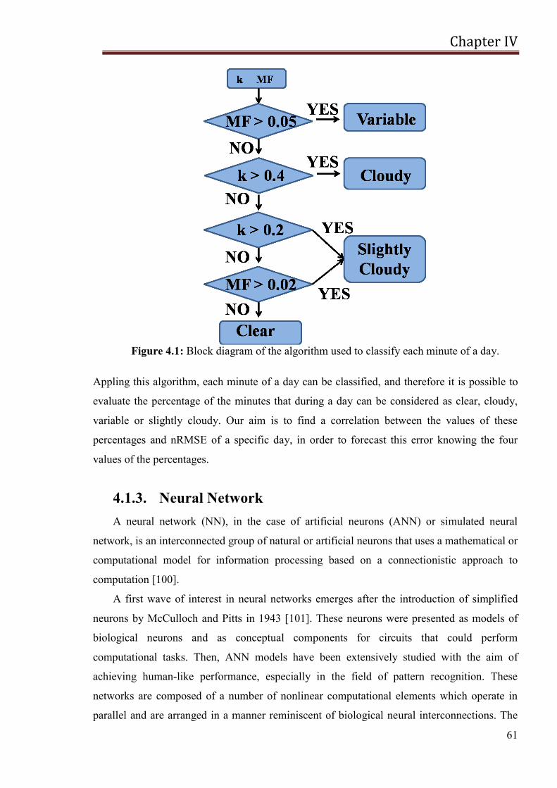
Chapter IV

61

Figure 4.1: Block diagram of the algorithm used to classify each minute of a day.

Appling this algorithm, each minute of a day can be classified, and therefore it is possible to

evaluate the percentage of the minutes that during a day can be considered as clear, cloudy,

variable or slightly cloudy. Our aim is to find a correlation between the values of these

percentages and nRMSE of a specific day, in order to forecast this error knowing the four

values of the percentages.

4.1.3. Neural Network

A neural network (NN), in the case of artificial neurons (ANN) or simulated neural

network, is an interconnected group of natural or artificial neurons that uses a mathematical or

computational model for information processing based on a connectionistic approach to

computation [100].

A first wave of interest in neural networks emerges after the introduction of simplified

neurons by McCulloch and Pitts in 1943 [101]. These neurons were presented as models of

biological neurons and as conceptual components for circuits that could perform

computational tasks. Then, ANN models have been extensively studied with the aim of

achieving human-like performance, especially in the field of pattern recognition. These

networks are composed of a number of nonlinear computational elements which operate in

parallel and are arranged in a manner reminiscent of biological neural interconnections. The

Chapter IV

62

area of neural networks is nowadays considered from two main perspectives. The first

perspective is cognitive science [102], which is an interdisciplinary study of the mind. The

second perspective is connectionism, which is a theory of information processing and

identification [103].

Artificial neural networks can be most adequately characterized as ‗computational models‘

with particular properties such as the ability to adapt to learn, to generalize, or to cluster or

organize data, and which operation is based on parallel processing. They have been developed

as generalizations of mathematical models of human cognition or neural biology, based on the

assumptions that [104]:

1. information processing occurs at many simple elements called neurons;

2. signals are passed between neurons over connection links;

3. each connection link has an associated weight, which, in a typical neural net, multiplies

the signal transmitted;

4. each neuron applies an activation function (usually nonlinear) to its net input (sum of

weighted input signals) to determine its output signal.

A neural network is characterized by:

1. its pattern of connections between the neurons (called its architecture);

2. its method of determining the weights on the connections (called its training, or

learning, algorithm);

3. its activation function.

A neural net consists of a large number of simple processing elements called neurons, units,

cells, or nodes. Each neuron is connected to other neurons by means of directed

communication links, each with an associated weight. The weights represent information

being used by the net to solve a problem; they are adapted during use to improve

performance. The main idea is to achieve good performance via dense interconnection of

simple computational elements.

Each neuron has an internal state, called its activation or activity level, which is a

function of the inputs it has received. Typically, a neuron sends its activation as a signal to

several other neurons. It is important to note that a neuron can send only one signal at a time,

although that signal is broadcast to several other neurons.

Often, it is convenient to visualize neurons as arranged in layers and typically, neurons in

the same layer behave in the same manner. A single-layer net has one layer of connection

weights. Often, the units can be distinguished as input units, which receive signals from the

outside world, and output units, from which the response of the net can be read. In the typical

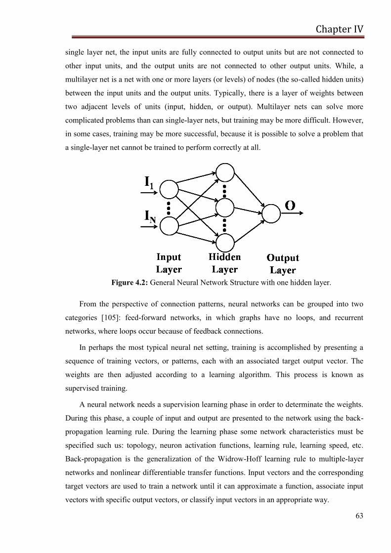
Chapter IV

63

single layer net, the input units are fully connected to output units but are not connected to

other input units, and the output units are not connected to other output units. While, a

multilayer net is a net with one or more layers (or levels) of nodes (the so-called hidden units)

between the input units and the output units. Typically, there is a layer of weights between

two adjacent levels of units (input, hidden, or output). Multilayer nets can solve more

complicated problems than can single-layer nets, but training may be more difficult. However,

in some cases, training may be more successful, because it is possible to solve a problem that

a single-layer net cannot be trained to perform correctly at all.

Figure 4.2: General Neural Network Structure with one hidden layer.

From the perspective of connection patterns, neural networks can be grouped into two

categories [105]: feed-forward networks, in which graphs have no loops, and recurrent

networks, where loops occur because of feedback connections.

In perhaps the most typical neural net setting, training is accomplished by presenting a

sequence of training vectors, or patterns, each with an associated target output vector. The

weights are then adjusted according to a learning algorithm. This process is known as

supervised training.

A neural network needs a supervision learning phase in order to determinate the weights.

During this phase, a couple of input and output are presented to the network using the back-

propagation learning rule. During the learning phase some network characteristics must be

specified such us: topology, neuron activation functions, learning rule, learning speed, etc.

Back-propagation is the generalization of the Widrow-Hoff learning rule to multiple-layer

networks and nonlinear differentiable transfer functions. Input vectors and the corresponding

target vectors are used to train a network until it can approximate a function, associate input

vectors with specific output vectors, or classify input vectors in an appropriate way.

Chapter IV

64

Therefore, the training of a network by back-propagation involves three stages: the feed-

forward of the input training pattern, the calculation and back-propagation of the associated

error, and the adjustment of the weights. After training, application of the net involves only

the computations of the feed-forward phase. Even if training is slow, a trained net can produce

its output very rapidly [104].

The classic approach to time series prediction is to undertake an analysis of the time

series data, which includes modeling, identification of the model and model parameter

estimation phases. The design may be iterated by measuring the closeness of the model to the

real data. This can be a long process, often involving the derivation, implementation and

refinement of a number of models before one with appropriate characteristics is found.

Neural nets can be applied to a wide variety of problems, such as storing and recalling

data or patterns, classifying patterns, performing general mappings from input patterns to

output patterns, grouping similar patterns, or finding solutions to constrained optimization

problems [104]. In particular, the most difficult systems to predict are: those with non-

stationary dynamics, where the underlying behavior varies with time, a typical example of

which is speech production; those which deal with physical data which are subject to noise

and experimentation error, such as biomedical signals; and those which deal with short time

series, providing few data points on which to conduct the analysis, such as heart rate signals,

chaotic signals and meteorological signals. In all these situations, traditional techniques are

severely limited. On the other hand, neural networks are powerful when applied to problems

whose solutions require knowledge which is difficult to specify, but for which there is an

abundance of examples.

4.1.3.1. Neural Network to approximate the nRMSE function

The neural network here implemented has been used to approximate the nRMSE

function.

The values of the learning period, size of data used in the training, neurons on the hidden

layer and learning rate were set on a trial and error basis. The neural network is composed by

four inputs that represent the four percentages of a specific day and one output that is the

correspondent nRMSE, while the number of neurons in the hidden-layer is set equal to ten

and the number of epochs equal to 3000. Moreover, a hyperbolic tangent sigmoid transfer

function is used as neuron activation function of the hidden layer, a linear transfer function is

used as the neuron activation function of the output layer, the learning rate is set equal to

Chapter IV

65

0.001 and the learning algorithm used to implement the neural network is the Levenberg-

Marquardt back-propagation. Using this algorithm the network trains function that updates

weight and bias values according to Levenberg-Marquardt optimization [106].

In this work, first the percentages calculated using measured data have been used as

input, then the nRMSE has been approximated having as inputs the four values of percentages

calculated using the forecast data.

4.1.4. Experimental Setup

First of all, in order to test the accuracy of the daily prediction of solar radiation, the

forecast data have been compared with the ground measured ones. In particular, data relative

to Catania (latitude 37°34

‘ N, longitude 15

°10

‘ E, Italy) have been considered.

4.1.4.1. Forecast Data

Meteorological data such as solar radiation, ambient temperature, relative humidity, wind

speed, clearness index and sunshine duration, are accepted as dependable and widely variable

sources. It is therefore required to be able to formulate forecasting and estimation models of

these meteorological data. These data play a very important role in PV systems [107].

However, in many cases, meteorological data forecasting can require the implementation

of complex algorithms. For this reason, in this paper forecast weather data, provided by

Datameteo, a historical provider, working in the field of data processing, monitoring, planning

and development of high performance services, in the world of meteorology, aeronautic,

nautical, environment, renewable energies and civil protection, has been used. This provider

uses the new 2 Km WRF EMM (Eulerian Mass Model) model. It derives from the framework

WRF with solver ARW and it is characterized by an extreme configurability and integrality

with other models. The atmospheric models simulate the evolution of the atmospheric

conditions on a three-dimensional grid with varying resolution, in conformity with the

necessities and use coordinates systems and different types of grid according to the

employment.

Datameteo provides us the following forecast measures: solar radiation, temperature,

wind speed and intensity, calculated in Catania (Italy); these data are provided as hourly data.

The provided flow of data is integrated by four modeling runs per day, but the updating

that are relevant for our target are only the first 72 hours of forecast that are updated by the 2

runs of the High resolution model; outputs are provided twice a day: at 9:30 a.m. and at 9:30

p.m.

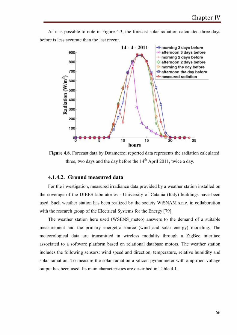
Chapter IV

66

As it is possible to note in Figure 4.3, the forecast solar radiation calculated three days

before is less accurate than the last recent.

Figure 4.8. Forecast data by Datameteo; reported data represents the radiation calculated

three, two days and the day before the 14th

April 2011, twice a day.

4.1.4.2. Ground measured data

For the investigation, measured irradiance data provided by a weather station installed on

the coverage of the DIEES laboratories - University of Catania (Italy) buildings have been

used. Such weather station has been realized by the society WiSNAM s.n.c. in collaboration

with the research group of the Electrical Systems for the Energy [79].

The weather station here used (WSENS_meteo) answers to the demand of a suitable

measurement and the primary energetic source (wind and solar energy) modeling. The

meteorological data are transmitted in wireless modality through a ZigBee interface

associated to a software platform based on relational database motors. The weather station

includes the following sensors: wind speed and direction, temperature, relative humidity and

solar radiation. To measure the solar radiation a silicon pyranometer with amplified voltage

output has been used. Its main characteristics are described in Table 4.1.

Chapter IV

67

Table 4.1: Silicon Pyranometer characteristics.

Spectral Range (10% points) 400 – 1100 nanometers

Cosine Response (% on reading) ±3% (from 0° to ± 70° incidence angle)

±10% (from ±70° to ±85° incidence angle)

Cosine Response (% on total range) ±2% (from 0° to ±90°)

Temperature Coefficient +0.12% per °C

Reference Temperature 25°C

Degree correction up the Reference

Temperature

+0.12% per °C

Accuracy 5% of end-scale value (Reference: Eppley PSP

to 1000 W/m2)

Sampling Time 1 minute

To have more complete and accurate information, an opportune conditioning circuit has been

positioned close to the silicon solar radiation sensor. This circuit allows to acquire (in the

same data structure) the signals relative to a reference solar radiation sensor based on the

thermopile working principle, Kipp&Zonen CM11.

Figure 4.9: Weather Station WSENSmeteo (the anemometer is placed at the top of a 4

m high pole).

A thermopile is a thermoelectric device that consists of an array of thermocouples

connected in series, less commonly, in parallel. It is widely used in non-contact temperature

measurement applications and temperature monitoring systems. Thermopiles detect the

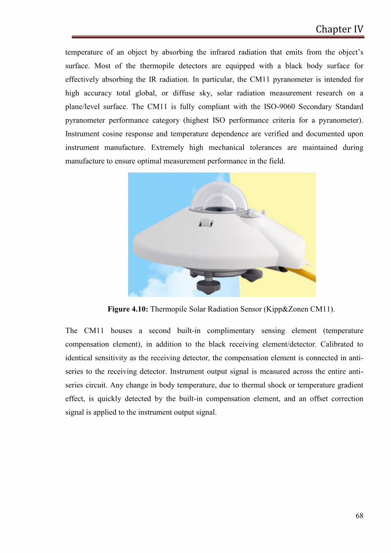
Chapter IV

68

temperature of an object by absorbing the infrared radiation that emits from the object‘s

surface. Most of the thermopile detectors are equipped with a black body surface for

effectively absorbing the IR radiation. In particular, the CM11 pyranometer is intended for

high accuracy total global, or diffuse sky, solar radiation measurement research on a

plane/level surface. The CM11 is fully compliant with the ISO-9060 Secondary Standard

pyranometer performance category (highest ISO performance criteria for a pyranometer).

Instrument cosine response and temperature dependence are verified and documented upon

instrument manufacture. Extremely high mechanical tolerances are maintained during

manufacture to ensure optimal measurement performance in the field.

Figure 4.10: Thermopile Solar Radiation Sensor (Kipp&Zonen CM11).

The CM11 houses a second built-in complimentary sensing element (temperature

compensation element), in addition to the black receiving element/detector. Calibrated to

identical sensitivity as the receiving detector, the compensation element is connected in anti-

series to the receiving detector. Instrument output signal is measured across the entire anti-

series circuit. Any change in body temperature, due to thermal shock or temperature gradient

effect, is quickly detected by the built-in compensation element, and an offset correction

signal is applied to the instrument output signal.

Chapter IV

69

Table 4.2: CM11 Pyranometer Specifications.

Spectral range (50% points) 305– 2800 nm

Sensitivity 4 - 6 μV/W/m2

Impedance (nominal) 700 - 1500 W

Response time (95%) 15 sec

Non-linearity < ± 0.6% (<1000 W/m2)

Temp. dependence of sensitivity < ± 1% (-10 to +40oC)

Directional error < ± 10 W/m2 (beam 1000 W/m2)

Tilt error None

Zero-offset due to temperature changes < ± 2 W/m2 at 5 K/h temperature change

Operating temperature -40oC to +80oC

ISO-9060 Class Secondary Standard

Dimensions W x H 150.0 mm x 91.5 mm

Weight 850 grams

Cable length 10 m

The receiving element is coated with a highly stable carbon based non-organic coating, which

delivers excellent spectral absorption and long term stability characteristics. The sensing

element is housed under two concentric fitting Schott K5 glass domes. Additional CM11

features include an integrated built-in bubble level, reusable desiccant drying cartridge, white

sunscreen, and a permanently attached shielded output signal cable. The CM11 can be used in

conjunction with the optional Kipp & Zonen CV2 ventilation system, for enhanced

measurement performance and overall reduced instrument maintenance.

4.1.5. Experimental Results

In Italy the third in-feed incentive mechanism (D.M 6 August 2010) has introduced an

increasing of the base tariff (+20%) connected with the programmability of the energy

produced by the PV plant. The owner of the PV power plant (the size of the PV system ranges

from 200 kW a 10 MW) has to respect an hourly scheduling (from 8:00 a.m. to 8:00 p.m.)

with a maximum forecast error of 10%. Further he has to communicate this forecasted

scheduling one day before the dispatching day.

In this study, an algorithm that allows to classify a day as clear, slightly cloudy, cloudy or

variable has been developed.

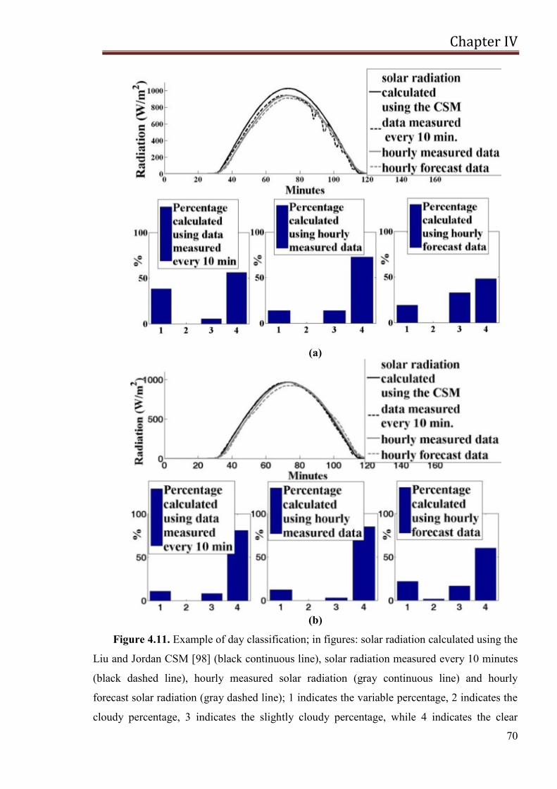
Chapter IV

70

(a)

(b)

Figure 4.11. Example of day classification; in figures: solar radiation calculated using the

Liu and Jordan CSM [98] (black continuous line), solar radiation measured every 10 minutes

(black dashed line), hourly measured solar radiation (gray continuous line) and hourly

forecast solar radiation (gray dashed line); 1 indicates the variable percentage, 2 indicates the

cloudy percentage, 3 indicates the slightly cloudy percentage, while 4 indicates the clear

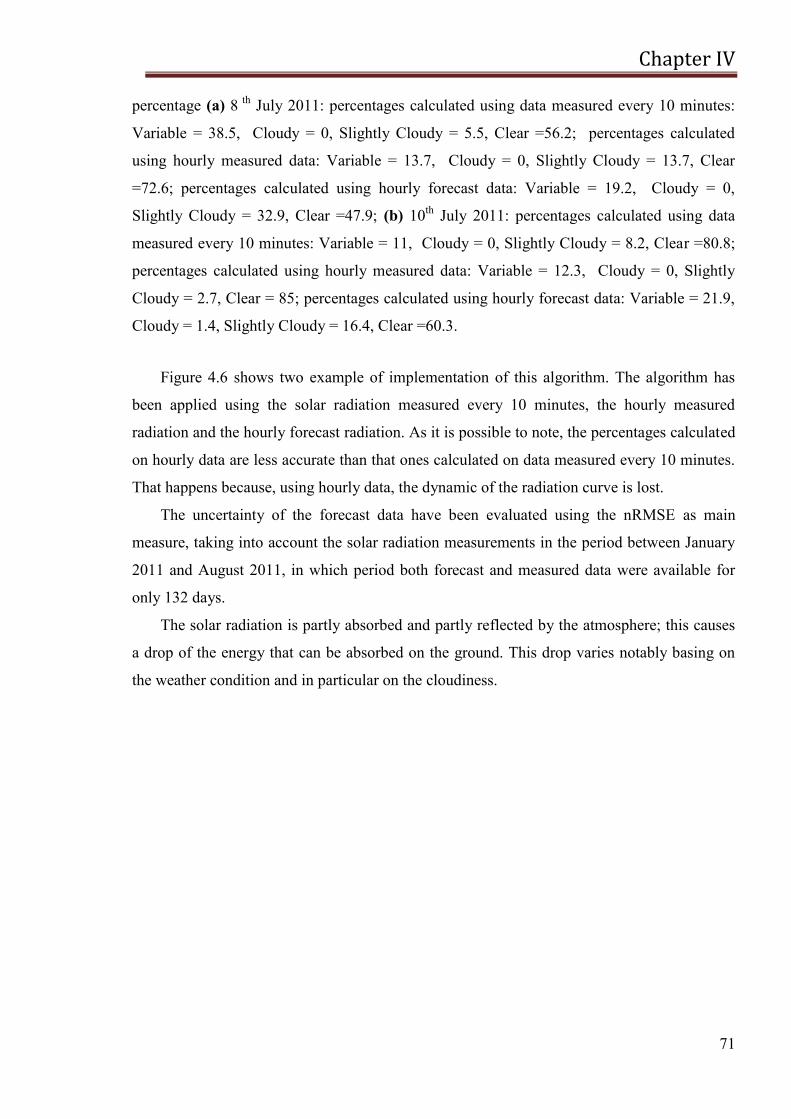
Chapter IV

71

percentage (a) 8 th

July 2011: percentages calculated using data measured every 10 minutes:

Variable = 38.5, Cloudy = 0, Slightly Cloudy = 5.5, Clear =56.2; percentages calculated

using hourly measured data: Variable = 13.7, Cloudy = 0, Slightly Cloudy = 13.7, Clear

=72.6; percentages calculated using hourly forecast data: Variable = 19.2, Cloudy = 0,

Slightly Cloudy = 32.9, Clear =47.9; (b) 10th

July 2011: percentages calculated using data

measured every 10 minutes: Variable = 11, Cloudy = 0, Slightly Cloudy = 8.2, Clear =80.8;

percentages calculated using hourly measured data: Variable = 12.3, Cloudy = 0, Slightly

Cloudy = 2.7, Clear = 85; percentages calculated using hourly forecast data: Variable = 21.9,

Cloudy = 1.4, Slightly Cloudy = 16.4, Clear =60.3.

Figure 4.6 shows two example of implementation of this algorithm. The algorithm has

been applied using the solar radiation measured every 10 minutes, the hourly measured

radiation and the hourly forecast radiation. As it is possible to note, the percentages calculated

on hourly data are less accurate than that ones calculated on data measured every 10 minutes.

That happens because, using hourly data, the dynamic of the radiation curve is lost.

The uncertainty of the forecast data have been evaluated using the nRMSE as main

measure, taking into account the solar radiation measurements in the period between January

2011 and August 2011, in which period both forecast and measured data were available for

only 132 days.

The solar radiation is partly absorbed and partly reflected by the atmosphere; this causes

a drop of the energy that can be absorbed on the ground. This drop varies notably basing on

the weather condition and in particular on the cloudiness.

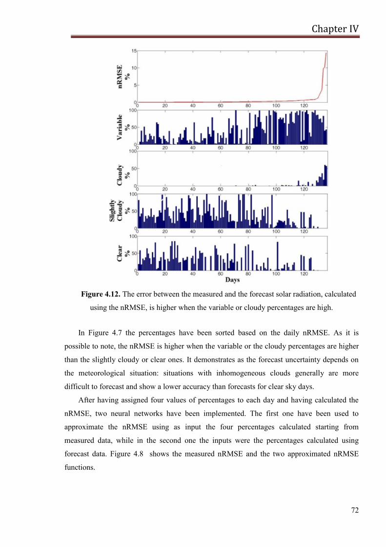
Chapter IV

72

Figure 4.12. The error between the measured and the forecast solar radiation, calculated

using the nRMSE, is higher when the variable or cloudy percentages are high.

In Figure 4.7 the percentages have been sorted based on the daily nRMSE. As it is

possible to note, the nRMSE is higher when the variable or the cloudy percentages are higher

than the slightly cloudy or clear ones. It demonstrates as the forecast uncertainty depends on

the meteorological situation: situations with inhomogeneous clouds generally are more

difficult to forecast and show a lower accuracy than forecasts for clear sky days.

After having assigned four values of percentages to each day and having calculated the

nRMSE, two neural networks have been implemented. The first one have been used to

approximate the nRMSE using as input the four percentages calculated starting from

measured data, while in the second one the inputs were the percentages calculated using

forecast data. Figure 4.8 shows the measured nRMSE and the two approximated nRMSE

functions.

Chapter IV

73

Figure 4.13: Comparison between the measured nRMSE and the approximated ones; in

figure: the star indicates the measured nRMSE, the circle indicates the nRMSE evaluated

through the neural network using the percentages calculated starting from measured data,

while triangle indicates the nRMSE evaluated through the neural network using the

percentages calculated starting from forecast data.

To evaluate the effectiveness of this approximation, the mean square error (MSE) has

been used:

(4.7)

where is the measured nRMSE, is the approximated one and N is the

number of the available days. For the first approximated function MSE was 0.0640, while for

the second one it was 0.9604.

As it is possible to note, the approximated function that uses the percentages calculated

starting from measured data is approximated better than the other one. Anyhow, the

approximated nRMSE functions calculated using the neural networks here implemented can

be considered a good approximation of the real one. Therefore, this neural network allows to

predict the value of the nRMSE of a specific day, the day before, using forecast data.

Chapter IV

74

4.2. Clear Sky Radiation Model on Horizontal

Surface

To calculate the index of serenity, Eq. 4.4, it is necessary to calculate the clear sky

radiation on the horizontal surface .

The maximum radiation is defined as the radiation occurring on days with a clear,

cloudless sky. For a cloudless sky, the global radiation takes maximum values. The maximum

global radiation corresponds to the greatest possible value of global radiation per hour at the

specified altitude [108].

Since there are a several number of variables to be calculated and they are unpredictable,

an accurate evaluation of the solar radiation, even if it is a clear sky day, is next to never

possible. Nonetheless, numerous methods have been developed to calculate the clear sky solar

radiation. These methods allow to have a degree of accuracy that can be considered

acceptable when this information must be used by engineers or architects. Among these

methods, the most used is the approach developed by Threlkeld and Jordan, used by the

ASHRAE [109] and modified by Iqbal [110], that is based on the calculation of solar

radiation through some simple algorithms that evaluate separately the effect that the

atmosphere have on the direct and diffuse solar radiation.

Solar flux striking a collector will be a combination of direct-beam radiation that passes

in a straight line through the atmosphere to the receiver, diffuse radiation that has been

scattered by molecules and aerosols in the atmosphere and reflected radiation that has

bounced off the ground or other surface in front of the collector [5] (Figure 4.9).

On a horizontal surface the reflected radiation is zero, therefore the total radiation is

given by the sum of direct ( ) and diffuse radiation ( ).

(4.8)

4.2.1. Clear sky direct-beam radiation

The direct or beam radiation is the solar radiation received from the sun without having

been scattered by the atmosphere. It comes in a direct line from the sun and therefore for

sunny days with clear skies, most of the solar radiation is direct beam radiation, while on

overcast days, the sun is obscured by the clouds and the direct beam radiation is zero.

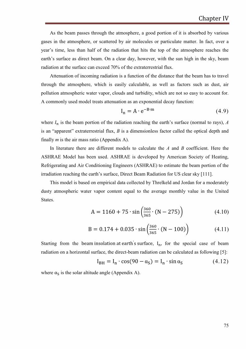
Chapter IV

75

As the beam passes through the atmosphere, a good portion of it is absorbed by various

gases in the atmosphere, or scattered by air molecules or particulate matter. In fact, over a

year‘s time, less than half of the radiation that hits the top of the atmosphere reaches the

earth‘s surface as direct beam. On a clear day, however, with the sun high in the sky, beam

radiation at the surface can exceed 70% of the extraterrestrial flux.

Attenuation of incoming radiation is a function of the distance that the beam has to travel

through the atmosphere, which is easily calculable, as well as factors such as dust, air

pollution atmospheric water vapor, clouds and turbidity, which are not so easy to account for.

A commonly used model treats attenuation as an exponential decay function:

(4.9)

where is the beam portion of the radiation reaching the earth‘s surface (normal to rays), A

is an ―apparent‖ extraterrestrial flux, B is a dimensionless factor called the optical depth and

finally m is the air mass ratio (Appendix A).

In literature there are different models to calculate the A and B coefficient. Here the

ASHRAE Model has been used. ASHRAE is developed by American Society of Heating,

Refrigerating and Air Conditioning Engineers (ASHRAE) to estimate the beam portion of the

irradiation reaching the earth‘s surface, Direct Beam Radiation for US clear sky [111].

This model is based on empirical data collected by Threlkeld and Jordan for a moderately

dusty atmospheric water vapor content equal to the average monthly value in the United

States.

(4.10)

(4.11)

Starting from the , for the special case of beam

radiation on a horizontal surface, the direct-beam radiation can be calculated as following [5]:

(4.12)

where is the solar altitude angle (Appendix A).

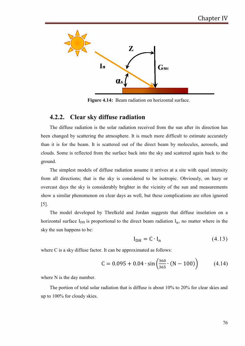
Chapter IV

76

Figure 4.14: Beam radiation on horizontal surface.

4.2.2. Clear sky diffuse radiation

The diffuse radiation is the solar radiation received from the sun after its direction has

been changed by scattering the atmosphere. It is much more difficult to estimate accurately

than it is for the beam. It is scattered out of the direct beam by molecules, aerosols, and

clouds. Some is reflected from the surface back into the sky and scattered again back to the

ground.

The simplest models of diffuse radiation assume it arrives at a site with equal intensity

from all directions; that is the sky is considered to be isotropic. Obviously, on hazy or

overcast days the sky is considerably brighter in the vicinity of the sun and measurements

show a similar phenomenon on clear days as well, but these complications are often ignored

[5].

The model developed by Threlkeld and Jordan suggests that diffuse insolation on a

horizontal surface IDH is proportional to the direct beam radiation , no matter where in the

sky the sun happens to be:

(4.13)

where C is a sky diffuse factor. It can be approximated as follows:

(4.14)

where N is the day number.

The portion of total solar radiation that is diffuse is about 10% to 20% for clear skies and

up to 100% for cloudy skies.

Chapter IV

77

4.3. Sub-hourly irradiance models on the plane

of array

The target of this section consists in the evaluation of models that estimate global solar

radiation on tilted plane based on that measured on horizontal surfaces. Simple methods can

be used for estimating beam and reflected components; in contrast, different models exist to

evaluate the diffuse one. These models need to split the horizontal global radiation into beam

and diffuse components. In this paper, a neural network, that allows to evaluate the global

solar radiation on a tilted surface directly from the horizontal one, has been developed.

4.3.1. Beam and diffuse components of hourly radiation

The split of total solar radiation on a horizontal surface into beam and diffuse

components is on interest in the context of calculating total radiation on surface of any

orientation and inclination from data measured on horizontal surface, where it is necessary

separate treatments of beam and diffuse radiation. To estimate the fraction of hourly radiation

on a horizontal plane which is diffuse, kd , different approaches can be used [112], where kd is

given by:

(4.15)

Of direct pertinence are the works of Orgill and Hollands [113], Reindl et al. [114],

Boland et al. [115], Hawlader [116], Miguel et al. [117], Karatasou et al. [118], Erbs et al.

[119], Chandrasekaran and Kumar [120], Oliveira et al. [121], and Soares et al. [122], who

established hourly correlations between and under diverse climatic conditions, where is

the clearness index. The models can be categorized as: first order ([113, 114, 115]), second-

third-order ([116, 117, 118]), and fourth-order ([119, 120, 121, 122]) correlations.

In [123] they have searched a possible relation between the diffuse component and the

hourly horizontal global irradiation.

Chapter IV

78

(a)

(b)

(c)

Figure 4.15: The hourly diffuse fraction versus clearness index , showing standard

and proposed correlations [123]: (a) first-order; (b) second–third order; and (c) fourth-order

polynomial correlations.

Chapter IV

79

In their studies seven relations have been applied, validated and compared using

statistical test parameters to quantify their accuracy. These studies confirmed the observations

previously described by Iqbal [124], Skartveit and Olseth [125] and De Miguel et al. [117]

concerning the influence of solar elevation on the correlation between diffuse and global

hourly irradiations; they have concluded that it appears, for the meteorological station of

Ajaccio-Vignola, that the model showing the best performances for solar data is the

CLIMED2 model [117], which in their work has been elaborated on the basis of solar data

collected in three Mediterranean stations.

Since in this work the same data relative to Ajaccio-Vignola have been used to test the

models here developed, the model, called CLIMED2, has been used. It has been developed by

De Miguel et al. [117] who have evaluated a series of models on 11 various sites of the

Mediterranean belt and on the basis of the data collected in these Mediterranean sites they

have found these correlations:

(4.16)

4.3.2. Solar Radiation on Inclined Surface

Historically, at many national meteorological stations, global irradiance has been

measured only on horizontal surfaces and rarely on inclined ones. Thus different methods

have been developed to estimate radiation on tilted surfaces from radiation on horizontal ones.

Actually, the total radiation incident on a tilted plane consists of three components:

beam radiation ( ), diffuse radiation ( ) and reflected radiation from the ground ( ):

(4.17)

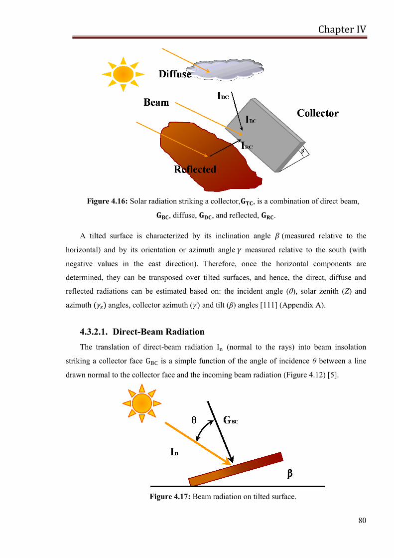
Chapter IV

80

Figure 4.16: Solar radiation striking a collector, , is a combination of direct beam,

, diffuse, , and reflected, .

A tilted surface is characterized by its inclination angle (measured relative to the

horizontal) and by its orientation or azimuth angle measured relative to the south (with

negative values in the east direction). Therefore, once the horizontal components are

determined, they can be transposed over tilted surfaces, and hence, the direct, diffuse and

reflected radiations can be estimated based on: the incident angle (θ), solar zenith (Z) and

azimuth angles, collector azimuth ( and tilt (β) angles [111] (Appendix A).

4.3.2.1. Direct-Beam Radiation

The translation of direct-beam radiation (normal to the rays) into beam insolation

striking a collector face is a simple function of the angle of incidence θ between a line

drawn normal to the collector face and the incoming beam radiation (Figure 4.12) [5].

Figure 4.17: Beam radiation on tilted surface.

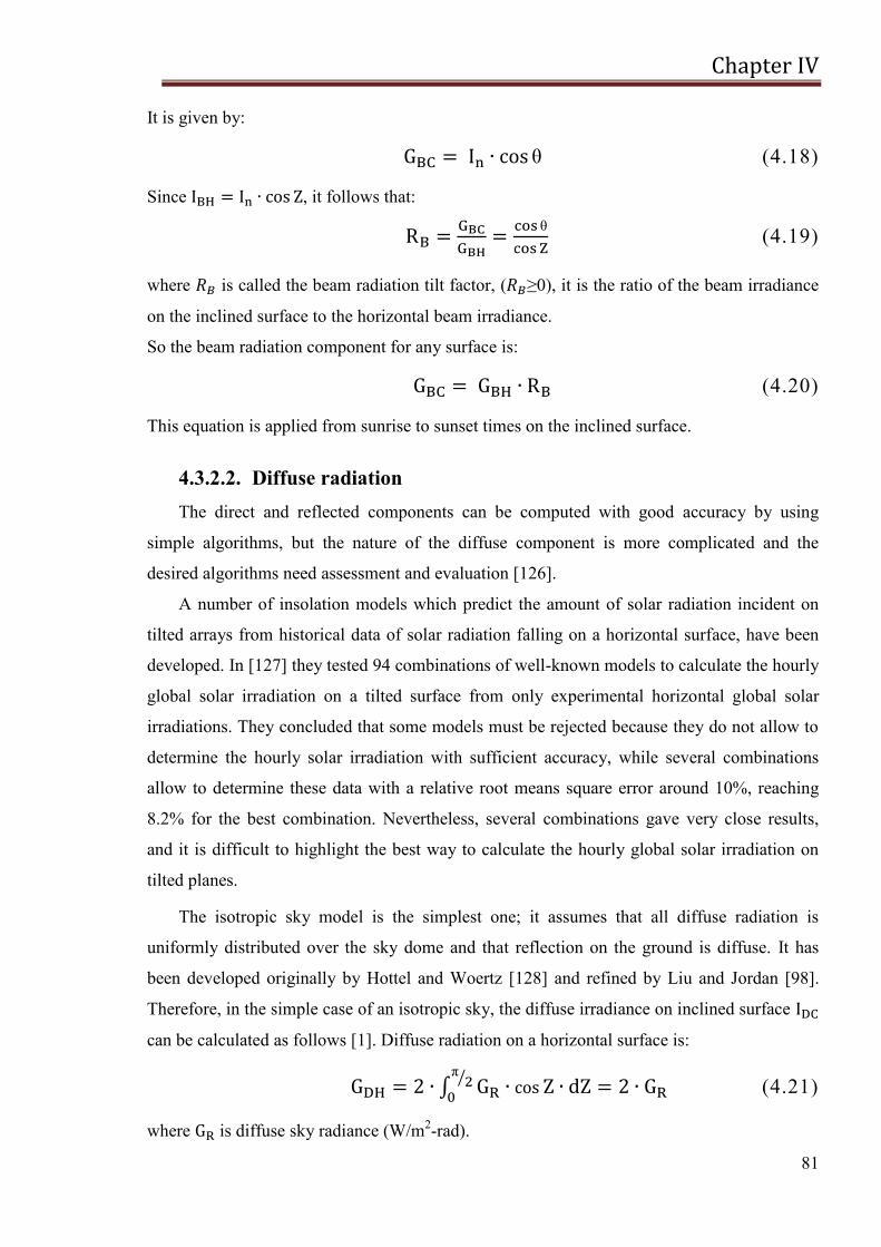
Chapter IV

81

It is given by:

θ (4.18)

Since , it follows that:

θ

(4.19)

where is called the beam radiation tilt factor, ( ≥0), it is the ratio of the beam irradiance

on the inclined surface to the horizontal beam irradiance.

So the beam radiation component for any surface is:

(4.20)

This equation is applied from sunrise to sunset times on the inclined surface.

4.3.2.2. Diffuse radiation

The direct and reflected components can be computed with good accuracy by using

simple algorithms, but the nature of the diffuse component is more complicated and the

desired algorithms need assessment and evaluation [126].

A number of insolation models which predict the amount of solar radiation incident on

tilted arrays from historical data of solar radiation falling on a horizontal surface, have been

developed. In [127] they tested 94 combinations of well-known models to calculate the hourly

global solar irradiation on a tilted surface from only experimental horizontal global solar

irradiations. They concluded that some models must be rejected because they do not allow to

determine the hourly solar irradiation with sufficient accuracy, while several combinations

allow to determine these data with a relative root means square error around 10%, reaching

8.2% for the best combination. Nevertheless, several combinations gave very close results,

and it is difficult to highlight the best way to calculate the hourly global solar irradiation on

tilted planes.

The isotropic sky model is the simplest one; it assumes that all diffuse radiation is

uniformly distributed over the sky dome and that reflection on the ground is diffuse. It has

been developed originally by Hottel and Woertz [128] and refined by Liu and Jordan [98].

Therefore, in the simple case of an isotropic sky, the diffuse irradiance on inclined surface

can be calculated as follows [1]. Diffuse radiation on a horizontal surface is:

(4.21)

where is diffuse sky radiance (W/m2-rad).

Chapter IV

82

While diffuse radiation on a tilted surface is:

β

(4.22)

where β is the surface tilt angle.

From Eq. 4.22, the second term of Eq. 4.23 becomes

.

Therefore, Eq. 4.23 becomes:

β

β

(4.23)

However, in reality, the radiance distribution of the sky is not isotropic. Therefore, an

anisotropic diffuse sky model must be used to accurately estimate the irradiance on the

inclined surface. In this work, we have implemented the Perez and the Klucher models

because they seem to be those having the best results; we have used data measured every ten

minutes and not hourly data.

In the Klucher model to calculate the diffuse irradiance on the tilted surface of the PV

array, the following equations are used [129]:

β

β

(4.24)

(4.25)

(4.26)

In [130, 131] Perez et al. developed a new, more accurate and considerably simpler

version of the Perez diffuse irradiance model [132]. This model is one of those used to

estimate short time step (hourly or less) irradiance on tilted planes based on global and direct

(or diffuse) irradiance. It has been shown to perform more accurately than other models for a

large number of locations worldwide.

Feuermann and Zemel [133] have shown that a combined application of the Perez et al.

model with empirical correlations to estimate the direct component from horizontal global

irradiance, can yield accurate predictions for locations where only global horizontal data are

available.

Chapter IV

83

The diffuse celestial radiation is divided into the components circumsolar, isotropic and

horizontal ribbon; the model governing the equation for diffuse celestial irradiance is:

β

β (4.27)

The terms a and b are given below:

θ

where is the incidence angle, while Z is the zenith angle.

In the slope irradiance model developed by Perez et al. [132], the circumsolar and the

horizon/zenith anisotropy are controlled by the dimensionless coefficients F1 and F2,

respectively. These are coefficients expressing the degree of circumsolar anisotropy and

anisotropy at the horizon/zenith respectively, are functions of the sky's clearness , the sky's

brightness , and the solar zenith angle Z.

The sky's clearness is defined by the equation below [57]:

(4.28)

where is the normal incidence beam irradiance and Z is expressed in radians.

The sky's brightness, noted as , is given by [140]:

(4.29)

where m is the relative optical air mass and is the normal incidence extraterrestrial

irradiance (Appendix A).

The variations of horizon and circumsolar brightening coefficients F1 and F2 with

insolation conditions have been observed to be consistent from site to site [134, 135]. They

can be calculated by the following equations:

(4.30)

The F11, F12, F13, F21, F22 and F23 coefficients can be chosen from Table 4.4 or Table 4.5.

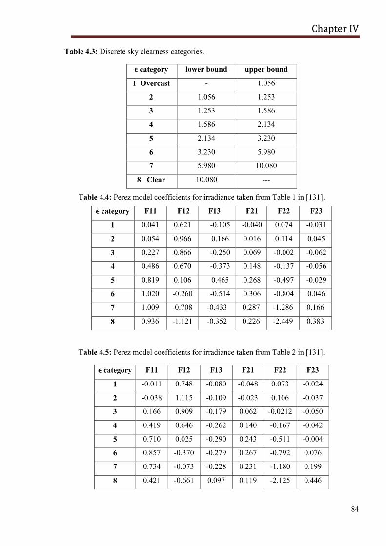
Chapter IV

84

Table 4.3: Discrete sky clearness categories.

category lower bound upper bound

1 Overcast - 1.056

2 1.056 1.253

3 1.253 1.586

4 1.586 2.134

5 2.134 3.230

6 3.230 5.980

7 5.980 10.080

8 Clear 10.080 ---

Table 4.4: Perez model coefficients for irradiance taken from Table 1 in [131].

category F11 F12 F13 F21 F22 F23

1 0.041 0.621 -0.105 -0.040 0.074 -0.031

2 0.054 0.966 0.166 0.016 0.114 0.045

3 0.227 0.866 -0.250 0.069 -0.002 -0.062

4 0.486 0.670 -0.373 0.148 -0.137 -0.056

5 0.819 0.106 0.465 0.268 -0.497 -0.029

6 1.020 -0.260 -0.514 0.306 -0.804 0.046

7 1.009 -0.708 -0.433 0.287 -1.286 0.166

8 0.936 -1.121 -0.352 0.226 -2.449 0.383

Table 4.5: Perez model coefficients for irradiance taken from Table 2 in [131].

category F11 F12 F13 F21 F22 F23

1 -0.011 0.748 -0.080 -0.048 0.073 -0.024

2 -0.038 1.115 -0.109 -0.023 0.106 -0.037

3 0.166 0.909 -0.179 0.062 -0.0212 -0.050

4 0.419 0.646 -0.262 0.140 -0.167 -0.042

5 0.710 0.025 -0.290 0.243 -0.511 -0.004

6 0.857 -0.370 -0.279 0.267 -0.792 0.076

7 0.734 -0.073 -0.228 0.231 -1.180 0.199

8 0.421 -0.661 0.097 0.119 -2.125 0.446

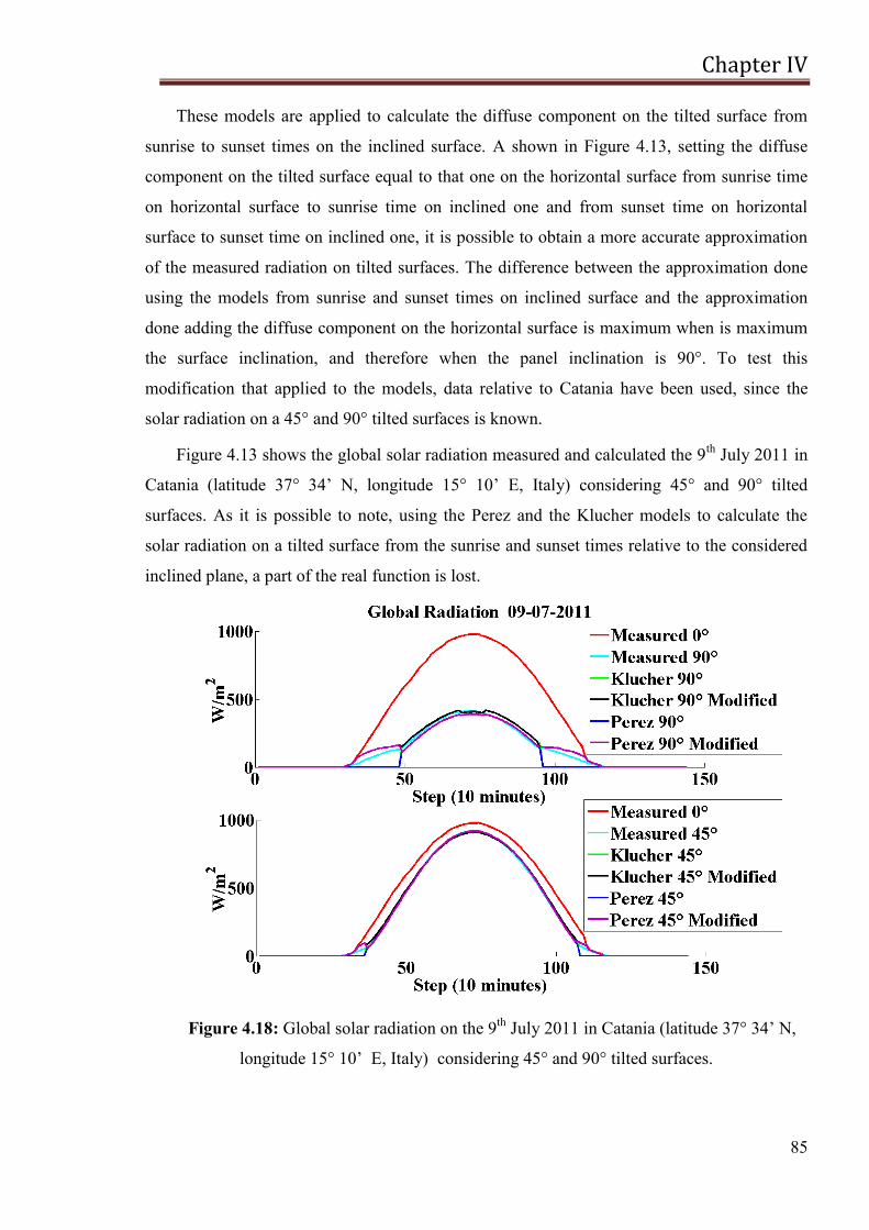
Chapter IV

85

These models are applied to calculate the diffuse component on the tilted surface from

sunrise to sunset times on the inclined surface. A shown in Figure 4.13, setting the diffuse

component on the tilted surface equal to that one on the horizontal surface from sunrise time

on horizontal surface to sunrise time on inclined one and from sunset time on horizontal

surface to sunset time on inclined one, it is possible to obtain a more accurate approximation

of the measured radiation on tilted surfaces. The difference between the approximation done

using the models from sunrise and sunset times on inclined surface and the approximation

done adding the diffuse component on the horizontal surface is maximum when is maximum

the surface inclination, and therefore when the panel inclination is 90°. To test this

modification that applied to the models, data relative to Catania have been used, since the

solar radiation on a 45° and 90° tilted surfaces is known.

Figure 4.13 shows the global solar radiation measured and calculated the 9th

July 2011 in

Catania (latitude 37° 34‘ N, longitude 15° 10‘ E, Italy) considering 45° and 90° tilted

surfaces. As it is possible to note, using the Perez and the Klucher models to calculate the

solar radiation on a tilted surface from the sunrise and sunset times relative to the considered

inclined plane, a part of the real function is lost.

Figure 4.18: Global solar radiation on the 9th

July 2011 in Catania (latitude 37° 34‘ N,

longitude 15° 10‘ E, Italy) considering 45° and 90° tilted surfaces.

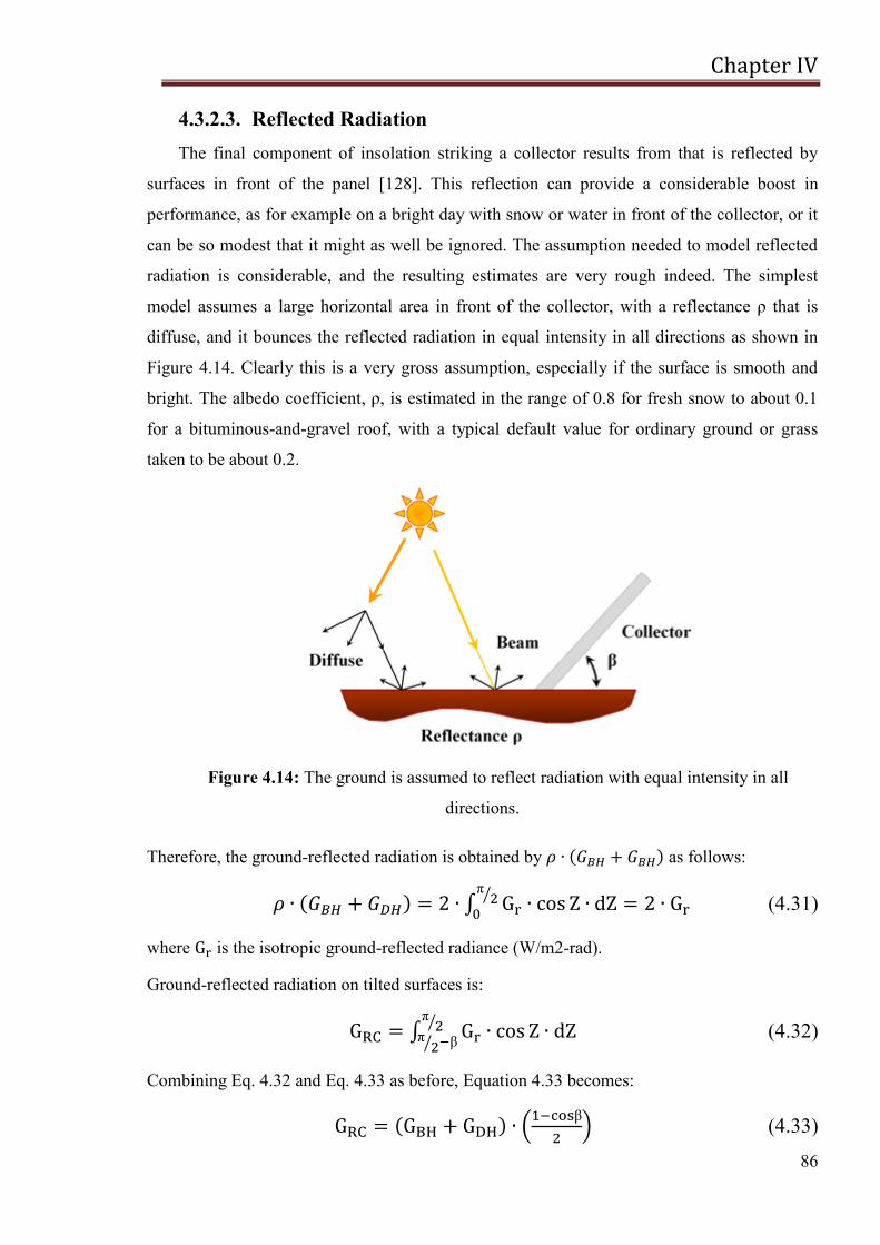
Chapter IV

86

4.3.2.3. Reflected Radiation

The final component of insolation striking a collector results from that is reflected by

surfaces in front of the panel [128]. This reflection can provide a considerable boost in

performance, as for example on a bright day with snow or water in front of the collector, or it

can be so modest that it might as well be ignored. The assumption needed to model reflected

radiation is considerable, and the resulting estimates are very rough indeed. The simplest

model assumes a large horizontal area in front of the collector, with a reflectance ρ that is

diffuse, and it bounces the reflected radiation in equal intensity in all directions as shown in

Figure 4.14. Clearly this is a very gross assumption, especially if the surface is smooth and

bright. The albedo coefficient, ρ, is estimated in the range of 0.8 for fresh snow to about 0.1

for a bituminous-and-gravel roof, with a typical default value for ordinary ground or grass

taken to be about 0.2.

Figure 4.14: The ground is assumed to reflect radiation with equal intensity in all

directions.

Therefore, the ground-reflected radiation is obtained by as follows:

(4.31)

where is the isotropic ground-reflected radiance (W/m2-rad).

Ground-reflected radiation on tilted surfaces is:

β (4.32)

Combining Eq. 4.32 and Eq. 4.33 as before, Equation 4.33 becomes:

β

(4.33)

Chapter IV

87

This equation is applied from sunrise to sunset times on the inclined surface.

4.3.3. Neural Network to approximate diffuse radiation on a tilted

surface

The neural network here implemented allows to approximate the solar radiation on a

tilted surface starting from the solar radiation on the horizontal plane.

It is composed by one inputs that represents the radiation on the horizontal plane and one

output that is the correspondent solar radiation on the 45° or 60° tilted surfaces, while the

number of neurons in the hidden-layer is set equal to 10 and the number of epochs equal to

100. Moreover, a hyperbolic tangent sigmoid transfer function is used as neuron activation

function of the hidden layer, a linear transfer function is used as the neuron activation

function of the output layer, the learning rate is set equal to 0.001 and the learning algorithm

used to implement the neural network is the Levenberg-Marquardt back-propagation [106].

4.3.4. Experimental Setup

To evaluate the performance of the solutions here adopted, we have used data provided

by the Laboratory "Systèmes Physiques de l'Environnement", Universitè de Corse Pascal

Paoli, Ajaccio, France [123]. In Ajaccio (Corsica, France), a seaside Mediterranean site

(Latitude 41°55° N, Longitude: 8°48°E), they have a complete meteorological station where

the normal beam irradiance is measured by an Eppley NIP pyrheliometer and the global

irradiances on horizontal, 45° or 60° tilted surfaces are measured by a Kipp & Zonen (CM11)

pyranometer. Other parameters such as temperature, pressure, relative humidity and wind

speed and direction, are also recorded. The data are collected and recorded every minute.

About 5% of the data values are missing because of some problems with the instruments and

some defects and maintenance in the data acquisition system.

The global radiations on the horizontal and tilted surface that we use in the experiments

have a time step of ten minutes obtained from an integration of the corresponding solar

irradiance collected every minute. For this study, we have one year (year 2003) of solar data:

global radiation on horizontal surface and on 45° and 60° tilted surfaces.

4.3.5. Experimental Results

Data collected in Ajaccio have been used to test the Klucher and the Perez models and

the neural network here implemented, calculating the solar radiation on a 45° and 60° tilted

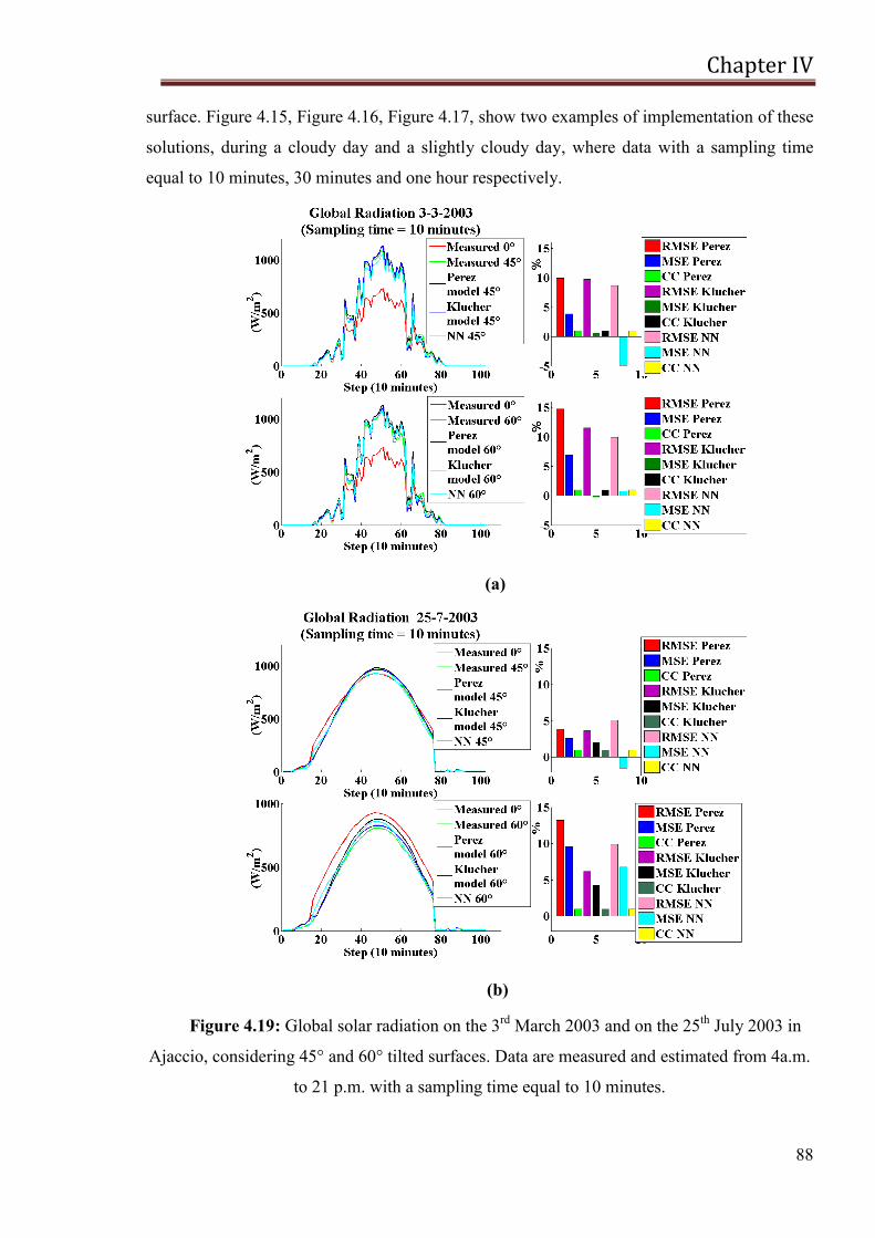
Chapter IV

88

surface. Figure 4.15, Figure 4.16, Figure 4.17, show two examples of implementation of these

solutions, during a cloudy day and a slightly cloudy day, where data with a sampling time

equal to 10 minutes, 30 minutes and one hour respectively.

(a)

(b)

Figure 4.19: Global solar radiation on the 3rd

March 2003 and on the 25th

July 2003 in

Ajaccio, considering 45° and 60° tilted surfaces. Data are measured and estimated from 4a.m.

to 21 p.m. with a sampling time equal to 10 minutes.

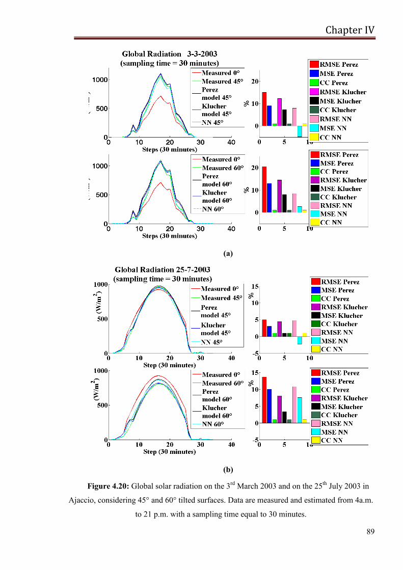
Chapter IV

89

(a)

(b)

Figure 4.20: Global solar radiation on the 3rd

March 2003 and on the 25th

July 2003 in

Ajaccio, considering 45° and 60° tilted surfaces. Data are measured and estimated from 4a.m.

to 21 p.m. with a sampling time equal to 30 minutes.

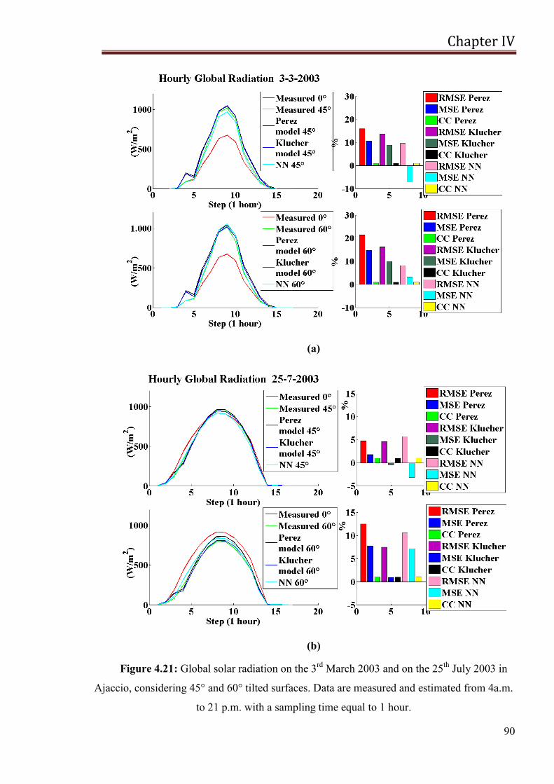
Chapter IV

90

(a)

(b)

Figure 4.21: Global solar radiation on the 3rd

March 2003 and on the 25th

July 2003 in

Ajaccio, considering 45° and 60° tilted surfaces. Data are measured and estimated from 4a.m.

to 21 p.m. with a sampling time equal to 1 hour.

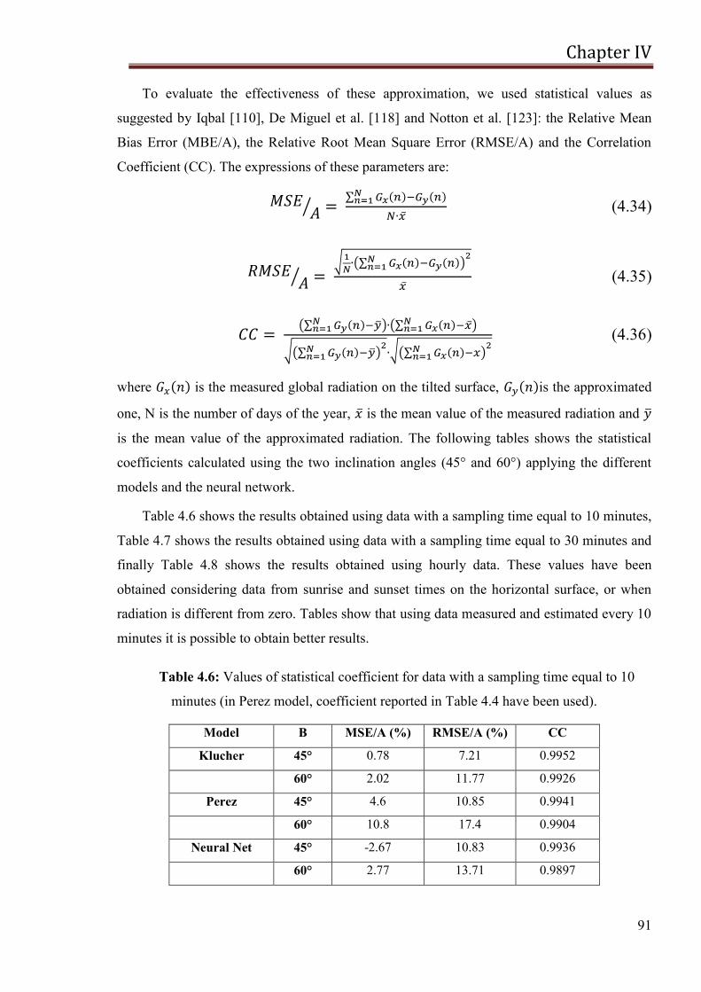
Chapter IV

91

To evaluate the effectiveness of these approximation, we used statistical values as

suggested by Iqbal [110], De Miguel et al. [118] and Notton et al. [123]: the Relative Mean

Bias Error (MBE/A), the Relative Root Mean Square Error (RMSE/A) and the Correlation

Coefficient (CC). The expressions of these parameters are:

(4.34)

(4.35)

(4.36)

where is the measured global radiation on the tilted surface, is the approximated

one, N is the number of days of the year, is the mean value of the measured radiation and

is the mean value of the approximated radiation. The following tables shows the statistical

coefficients calculated using the two inclination angles (45° and 60°) applying the different

models and the neural network.

Table 4.6 shows the results obtained using data with a sampling time equal to 10 minutes,

Table 4.7 shows the results obtained using data with a sampling time equal to 30 minutes and

finally Table 4.8 shows the results obtained using hourly data. These values have been

obtained considering data from sunrise and sunset times on the horizontal surface, or when

radiation is different from zero. Tables show that using data measured and estimated every 10

minutes it is possible to obtain better results.

Table 4.6: Values of statistical coefficient for data with a sampling time equal to 10

minutes (in Perez model, coefficient reported in Table 4.4 have been used).

Model Β MSE/A (%) RMSE/A (%) CC

Klucher 45° 0.78 7.21 0.9952

60° 2.02 11.77 0.9926

Perez 45° 4.6 10.85 0.9941

60° 10.8 17.4 0.9904

Neural Net 45° -2.67 10.83 0.9936

60° 2.77 13.71 0.9897

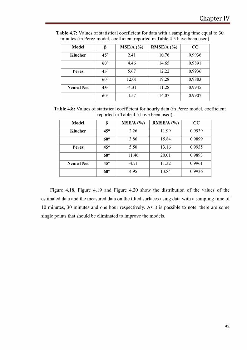
Chapter IV

92

Table 4.7: Values of statistical coefficient for data with a sampling time equal to 30

minutes (in Perez model, coefficient reported in Table 4.5 have been used).

Model β MSE/A (%) RMSE/A (%) CC

Klucher 45° 2.41 10.76 0.9936

60° 4.46 14.65 0.9891

Perez 45° 5.67 12.22 0.9936

60° 12.01 19.28 0.9883

Neural Net 45° -4.31 11.28 0.9945

60° 4.57 14.07 0.9907

Table 4.8: Values of statistical coefficient for hourly data (in Perez model, coefficient

reported in Table 4.5 have been used).

Model β MSE/A (%) RMSE/A (%) CC

Klucher 45° 2.26 11.99 0.9939

60° 3.86 15.84 0.9899

Perez 45° 5.50 13.16 0.9935

60° 11.46 20.01 0.9893

Neural Net 45° -4.71 11.32 0.9961

60° 4.95 13.84 0.9936

Figure 4.18, Figure 4.19 and Figure 4.20 show the distribution of the values of the

estimated data and the measured data on the tilted surfaces using data with a sampling time of

10 minutes, 30 minutes and one hour respectively. As it is possible to note, there are some

single points that should be eliminated to improve the models.

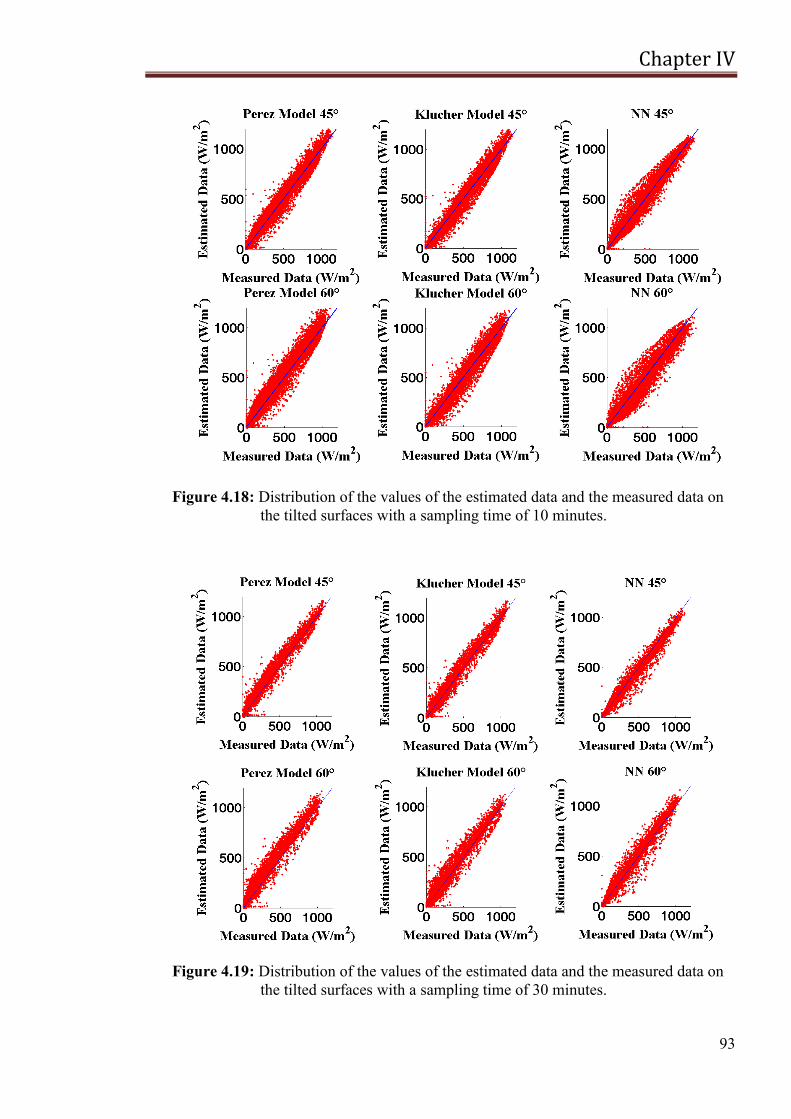
Chapter IV

93

Figure 4.18: Distribution of the values of the estimated data and the measured data on

the tilted surfaces with a sampling time of 10 minutes.

Figure 4.19: Distribution of the values of the estimated data and the measured data on

the tilted surfaces with a sampling time of 30 minutes.

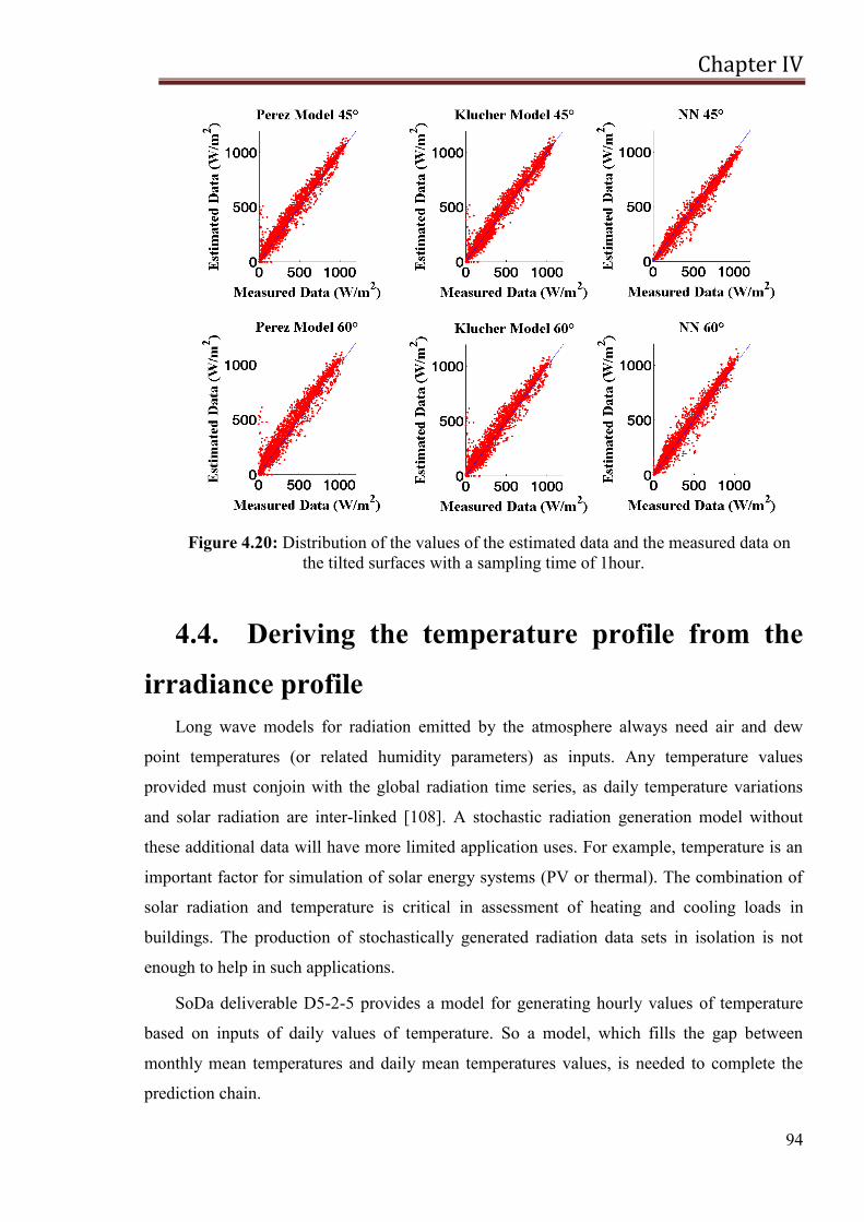
Chapter IV

94

Figure 4.20: Distribution of the values of the estimated data and the measured data on

the tilted surfaces with a sampling time of 1hour.

4.4. Deriving the temperature profile from the

irradiance profile

Long wave models for radiation emitted by the atmosphere always need air and dew

point temperatures (or related humidity parameters) as inputs. Any temperature values

provided must conjoin with the global radiation time series, as daily temperature variations

and solar radiation are inter-linked [108]. A stochastic radiation generation model without

these additional data will have more limited application uses. For example, temperature is an

important factor for simulation of solar energy systems (PV or thermal). The combination of

solar radiation and temperature is critical in assessment of heating and cooling loads in

buildings. The production of stochastically generated radiation data sets in isolation is not

enough to help in such applications.

SoDa deliverable D5-2-5 provides a model for generating hourly values of temperature

based on inputs of daily values of temperature. So a model, which fills the gap between

monthly mean temperatures and daily mean temperatures values, is needed to complete the

prediction chain.

Chapter IV

95

Here, a stochastic model for generating hourly values is used. Neither model helps solve the

given problem [108].

First, a term showing the response of the air temperature to the solar radiation input is

introduced. This ratio is called the ground to extraterrestrial irradiation ratio: kx. This is the

ratio of the amount of solar radiation received on the ground since sunrise, to the amount of

solar radiation that a surface perpendicular to the sunrays would have received during the

same period:

(4.37)

where:

GTC(t) is the global horizontal irradiance;

G0 is the solar constant: 1367 W /m2

It was shown that the variations of the temperature follow the variations of kx. The

temperature increases when kx increases. The temperature reaches its maximum value at the

same time as kx reaches its maximum (kxmax). When kx decreases, the temperature decreases.

It was concluded that during daylight hours the temperature varies linearly with the kx

coefficient. The slope of this linear relationship seems to depend on the sky conditions. It also

seems to be different before the maximum value of kx has been reached and afterwards.

Finally, it is certainly influenced by incoming air masses.

These conclusions lead to the following equation for the slope:

(4.38)

(4.39)

This slope is used to calculate the hourly temperature values during daytime:

if

(4.40)

During night the temperature variation is mainly influenced by the amount of clouds. To

characterize the sky conditions, the Perraudeau‘s nebulosity index has been used: IN

(Perraudeau, 1986) [78]. IN is based on the diffuse fraction and normalizes the value by

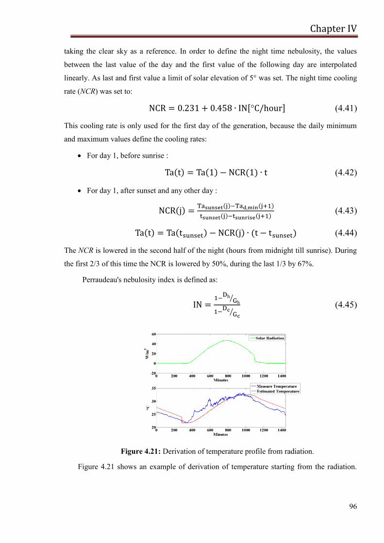
Chapter IV

96

taking the clear sky as a reference. In order to define the night time nebulosity, the values

between the last value of the day and the first value of the following day are interpolated

linearly. As last and first value a limit of solar elevation of 5° was set. The night time cooling

rate (NCR) was set to:

° (4.41)

This cooling rate is only used for the first day of the generation, because the daily minimum

and maximum values define the cooling rates:

For day 1, before sunrise :

(4.42)

For day 1, after sunset and any other day :

(4.43)

(4.44)

The NCR is lowered in the second half of the night (hours from midnight till sunrise). During

the first 2/3 of this time the NCR is lowered by 50%, during the last 1/3 by 67%.

Perraudeau's nebulosity index is defined as:

h h

(4.45)

Figure 4.21: Derivation of temperature profile from radiation.

Figure 4.21 shows an example of derivation of temperature starting from the radiation.

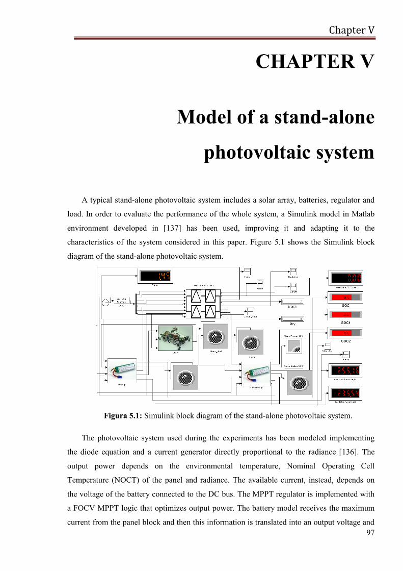
Chapter V

97

CHAPTER V

Model of a stand-alone

photovoltaic system

A typical stand-alone photovoltaic system includes a solar array, batteries, regulator and

load. In order to evaluate the performance of the whole system, a Simulink model in Matlab

environment developed in [137] has been used, improving it and adapting it to the

characteristics of the system considered in this paper. Figure 5.1 shows the Simulink block

diagram of the stand-alone photovoltaic system.

Figura 5.1: Simulink block diagram of the stand-alone photovoltaic system.

The photovoltaic system used during the experiments has been modeled implementing

the diode equation and a current generator directly proportional to the radiance [136]. The

output power depends on the environmental temperature, Nominal Operating Cell

Temperature (NOCT) of the panel and radiance. The available current, instead, depends on

the voltage of the battery connected to the DC bus. The MPPT regulator is implemented with

a FOCV MPPT logic that optimizes output power. The battery model receives the maximum

current from the panel block and then this information is translated into an output voltage and

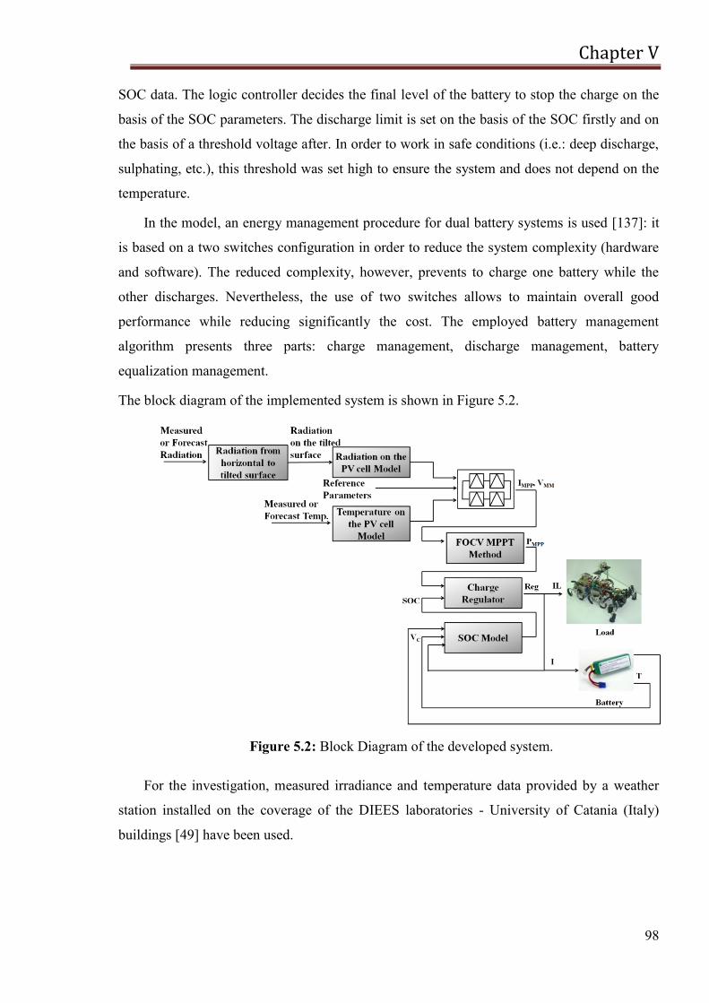
Chapter V

98

SOC data. The logic controller decides the final level of the battery to stop the charge on the

basis of the SOC parameters. The discharge limit is set on the basis of the SOC firstly and on

the basis of a threshold voltage after. In order to work in safe conditions (i.e.: deep discharge,

sulphating, etc.), this threshold was set high to ensure the system and does not depend on the

temperature.

In the model, an energy management procedure for dual battery systems is used [137]: it

is based on a two switches configuration in order to reduce the system complexity (hardware

and software). The reduced complexity, however, prevents to charge one battery while the

other discharges. Nevertheless, the use of two switches allows to maintain overall good

performance while reducing significantly the cost. The employed battery management

algorithm presents three parts: charge management, discharge management, battery

equalization management.

The block diagram of the implemented system is shown in Figure 5.2.

Figure 5.2: Block Diagram of the developed system.

For the investigation, measured irradiance and temperature data provided by a weather

station installed on the coverage of the DIEES laboratories - University of Catania (Italy)

buildings [49] have been used.

Chapter V

99

5.1. I-V characteristic generation

The analysis of the performance of a PV array needs basically the reporting the real

working conditions to a reference condition of irradiance and temperature. Normally it is used

the Standard Test Conditions (STC). In this context, in the following paragraphs, an analytical

model to evaluate the energy performance of an I-V characteristic under varying

meteorological conditions is proposed. The model is based on some data provided by the

manufacturer of the module.

Normally PV models are based on a electrical equivalent circuits where some parameters,

from three to seven depending on the complexity of the model, are unknown; the most

common electric circuit is made of the following elements: a current generator, a diode, a

series resistant and a shunt resistant; in this circuit there are five parameters. These parameters

can be evaluated by means of either numerical methods that minimize the difference between

a measured I-V curve and the one calculated by the model, or just using the technical data

provided by that manufacturer of the PV module. However the manufacturer of PV module

typically provide detailed information at only one operating condition, whereas PV modules

operate over large range of conditions so the information reported in datasheet are not

sufficient to determine their overall performance.

However this direct approach is very valuable as data sheets are always available and so

this model can be very easily built. In [138] a direct method is described but it uses the open

circuit voltage at 200 W/m2 that is a data that normally is not reported numerically in a

datasheet, sometimes there is a graph with I-V at different irradiance, but it is difficult to read

the open circuit voltage as the I-V curves are very close each other. Whereas, in [139], they

propose a direct method based on the use of five parameter electrical equivalent circuit. In this

case five independent pieces of information are needed. The most critical information used is

the temperature coefficient of the open circuit voltage. As this parameter, as well as other

thermal coefficients depend on the distribution of the temperature on the modules [140].

5.1.1. The reference parameters

In this context, to calculate the reference parameters, the five parameters method to

model the PV cells have been used. This model is relative to the equivalent circuit

representative either a PV cell or a PV module (Figure 5.3). It is a complete circuit where both

the sources of power losses are used RS and RSH.

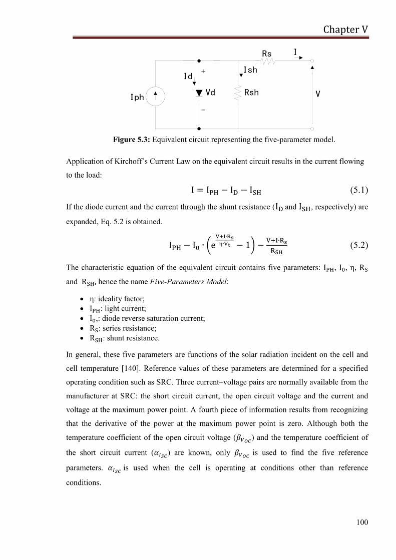
Chapter V

100

Figure 5.3: Equivalent circuit representing the five-parameter model.

Application of Kirchoff‘s Current Law on the equivalent circuit results in the current flowing

to the load:

(5.1)

If the diode current and the current through the shunt resistance ( and , respectively) are

expanded, Eq. 5.2 is obtained.

(5.2)

The characteristic equation of the equivalent circuit contains five parameters: , , ,

and hence the name Five-Parameters Model:

: ideality factor;

: light current;

,: diode reverse saturation current;

: series resistance;

: shunt resistance.

In general, these five parameters are functions of the solar radiation incident on the cell and

cell temperature [140]. Reference values of these parameters are determined for a specified

operating condition such as SRC. Three current–voltage pairs are normally available from the

manufacturer at SRC: the short circuit current, the open circuit voltage and the current and

voltage at the maximum power point. A fourth piece of information results from recognizing

that the derivative of the power at the maximum power point is zero. Although both the

temperature coefficient of the open circuit voltage ( ) and the temperature coefficient of

the short circuit current ( ) are known, only

is used to find the five reference

parameters. is used when the cell is operating at conditions other than reference

conditions.

+

-

Iph

Id

Vd V

Rs I

Rsh

Ish

Chapter V

101

To calculate the five parameters, Eq. 1 has to be calculated in the following three points:

open circuit ―OC‖, short circuit ―SC‖ and maximum power point ―MP‖. The expressions are

reported in Table 5.1.

Table 5.1: Expression of Eq. 5.2 in different operating points.

OC

(5.3)

SC

(5.4)

MP

(5.5)

Differentiating 5.2 with respect to V gives:

(5.6)

Calculating Eq. 5.2 at the maximum power point, we have:

(5.7)

Moreover, calculating Eq. 5.2 at short circuit:

(5.8)

Simultaneously solving Eq. 5.3 through 5.5, 5.7 and 5.8, it is possible to find the five

parameters in STC condition. Whatever is the irradiance and temperature, if the operating

points (voltage V and current I) at: open circuit, short circuit and maximum power are known,

it is possible to calculate the parameters. But the main point is that this approach has the

advantage to use input data that are always provided by the manufacturers such as: , ,

, and the PV cell temperature. In particular, these data refer to STC conditions,

=25°C and =1000 W/m2. In this case, these parameters are specified with a

lowercase ―ref ―: , ,

, and

.

Chapter V

102

The I-V curve varies with irradiance and cell temperature so, as matter of fact, also the

parameters will vary. In the following section the dependence of the parameters on operating

conditions is reported. Finally, the knowledge of the parameters allows to calculate the I-V

characteristic, using the W-Lambert function [141].

5.1.2. Dependence of the parameters on operating

conditions

Each parameter depends on the operating conditions and can be calculated starting from

the reference value.

From the definition of , the ideality factor is a linear function of cell temperature so that:

(5.9)

where and are the cell temperature and ideality factor for reference conditions,

while and are the cell temperature and ideality factor parameter for the new operating

conditions.

Messenger and Ventre in [142] present an equation from diode theory for the diode

reverse saturation current, I0. The ratio of their equation at the new operating temperature to

that at the reference temperature yields:

(5.10)

where k is Boltzmann constant and is the material band gap. exhibits a small

temperature dependence [143] which, for silicon, can be represented as indicated in Eq. 5.11

where for silicon cells.

(5.11)

The light current, (IPH), is nearly a linear function of incident solar radiation. Some

pyranometers, in fact, use the short circuit current of a solar cell as a measure of the incident

solar radiation. The light current (IPH) is observed to depend on the absorbed solar irradiance

(GC), the cell temperature ( ), the short circuit current temperature coefficient, , and the

air mass modifier (M). The light current IPH for any operating conditions is assumed to be

related to the light current at reference conditions by:

Chapter V

103

(5.12)

where , , and are the parameters at reference conditions, while G, M,

and are the values for specified operating conditions. When using Eq. 5.12 to find the

reference parameters, G= and M= . The air mass modifier is assumed to be a function

of the local zenith angle and is discussed below.

The final task to complete the model is to investigate the operating condition dependence

of the series resistance RS, and the shunt resistance, RSH. The series resistance impacts the

shape of current and voltage curve near the maximum power point. The effect on the I–V

curve is small and, although methods of adjusting RS as a function of operating conditions

have been investigated [144], RS is assumed constant at its reference value, in this

study.

(5.13)

The shunt resistance (RSH) controls the slope of the I–V curve at the short circuit condition;

large shunt resistances result in a horizontal slope. The shunt resistance appears to change

with absorbed solar radiation for all of the cells although the effect is most noticeable for cell

types that have a relatively small shunt resistance at SRC, such as the triple junction

amorphous cell [152]. If experimental data were generally available at more than one solar

radiation value, it would be possible to develop a relation between the shunt resistance and

absorbed radiation. However, this information is not normally available. Schroder in [145]

indicates that the shunt resistance is approximately inversely proportional to the short-circuit

current (and thus radiation) at very low light intensities.

(5.14)

5.1.2.1. The air mass modifier

Air mass is the ratio of the mass of air that the beam radiation has to traverse at any given

time and location to the mass of air that the beam radiation would traverse if the sun were

directly overhead. Selective absorption by species in the atmosphere causes the spectral

content of irradiance to change, altering the spectral distribution of the radiation incident on

the PV panel. King et al. [146] developed an empirical relation to account for air mass:

Chapter V

104

(5.15)

where AM is the air mass and is approximately given by:

(5.16)

where a0, a1, a2, a3, and a4 are constants for different PV materials which are available for

many cell types from Sandia National Laboratories [147]. While, Z is the Zenith angles,

values greater than 75° are generally associated with low solar radiation values and thus the

differences observed in the air mass modifiers for large angles are not important.

5.1.3. PV cells temperature and irradiance

The model of PV modules needs the following input:

Temperature of PV cells, ;

Irradiance on PV cells, .

Normally, both these variables cannot be measured directly but they can be calculated by

mathematical models based on both environmental variables (global irradiance, ambient

temperature and wind speed) and, in particular for T indirect measurements such as: backside

panel temperature and open circuit voltage.

5.1.3.1. Temperature of PV cells

The nominal operating cell temperature (NOCT) is commonly used to predict the cell

temperature over a range of environmental conditions. By definition, the NOCT is the

temperature of the cells at a solar irradiance of 800 W/m2, an ambient temperature of 20°C,

and a wind speed of 1m/s. The NOCT approach is based on the more common scenario where

both sides of the PV module see the same ambient temperature and wind conditions. Notably,

the approach also makes the approximation that the overall heat transfer coefficient for the PV

module is constant.

Alternative methods for predicting the cell temperature are based on the approximation of

one-dimensional, transient heat transfer. In these studies the panel is divided into three layers

[148, 149]): top cover, PV cells, and back layer. These two approaches have been compared

in [150], where the deviations due to different temperature sensors have been investigated in

laboratory tests and under real world conditions in an outdoor lab. The thermal behaviour is

studied and the measurements results are compared to theoretical models. One conclusion

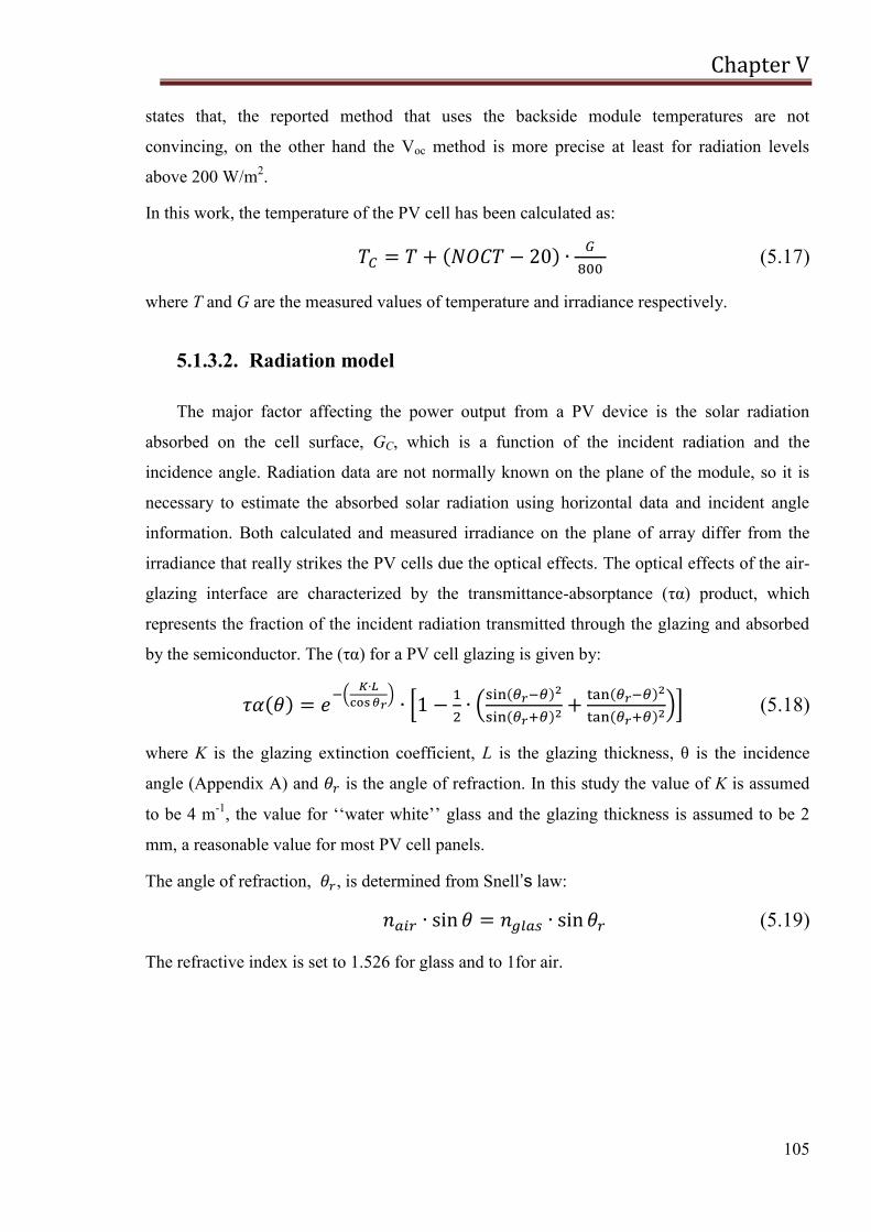
Chapter V

105

states that, the reported method that uses the backside module temperatures are not

convincing, on the other hand the Voc method is more precise at least for radiation levels

above 200 W/m2.

In this work, the temperature of the PV cell has been calculated as:

(5.17)

where T and G are the measured values of temperature and irradiance respectively.

5.1.3.2. Radiation model

The major factor affecting the power output from a PV device is the solar radiation

absorbed on the cell surface, GC, which is a function of the incident radiation and the

incidence angle. Radiation data are not normally known on the plane of the module, so it is

necessary to estimate the absorbed solar radiation using horizontal data and incident angle

information. Both calculated and measured irradiance on the plane of array differ from the

irradiance that really strikes the PV cells due the optical effects. The optical effects of the air-

glazing interface are characterized by the transmittance-absorptance (τ ) product, which

represents the fraction of the incident radiation transmitted through the glazing and absorbed

by the semiconductor. The (τ ) for a PV cell glazing is given by:

(5.18)

where K is the glazing extinction coefficient, L is the glazing thickness, θ is the incidence

angle (Appendix A) and is the angle of refraction. In this study the value of K is assumed

to be 4 m-1, the value for ‗‗water white‘‘ glass and the glazing thickness is assumed to be 2

mm, a reasonable value for most PV cell panels.

The angle of refraction, , is determined from Snell’s law:

(5.19)

The refractive index is set to 1.526 for glass and to 1for air.

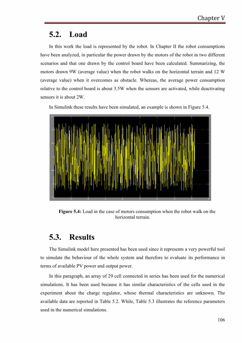
Chapter V

106

5.2. Load

In this work the load is represented by the robot. In Chapter II the robot consumptions

have been analyzed, in particular the power drawn by the motors of the robot in two different

scenarios and that one drawn by the control board have been calculated. Summarizing, the

motors drawn 9W (average value) when the robot walks on the horizontal terrain and 12 W

(average value) when it overcomes as obstacle. Whereas, the average power consumption

relative to the control board is about 3.5W when the sensors are activated, while deactivating

sensors it is about 2W.

In Simulink these results have been simulated, an example is shown in Figure 5.4.

Figure 5.4: Load in the case of motors consumption when the robot walk on the

horizontal terrain.

5.3. Results

The Simulink model here presented has been used since it represents a very powerful tool

to simulate the behaviour of the whole system and therefore to evaluate its performance in

terms of available PV power and output power.

In this paragraph, an array of 29 cell connected in series has been used for the numerical

simulations. It has been used because it has similar characteristics of the cells used in the

experiment about the charge regulator, whose thermal characteristics are unknown. The

available data are reported in Table 5.2. While, Table 5.3 illustrates the reference parameters

used in the numerical simulations.

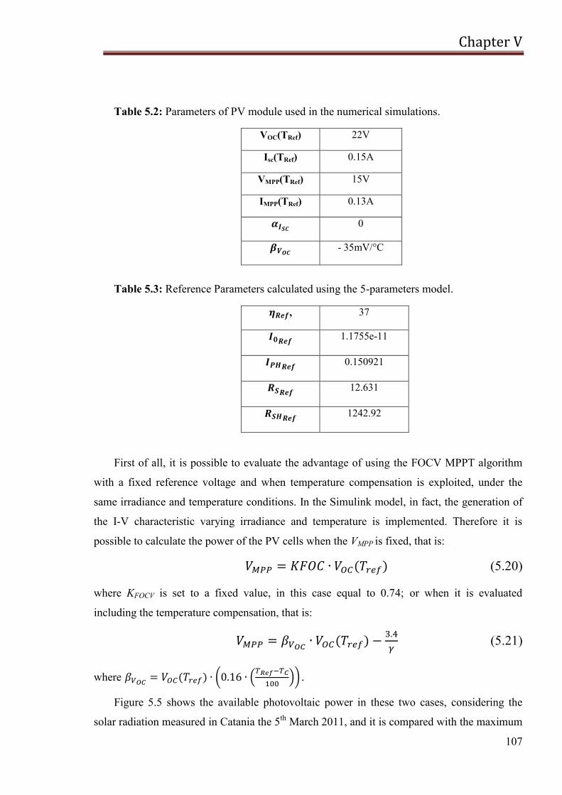
Chapter V

107

Table 5.2: Parameters of PV module used in the numerical simulations.

VOC(TRef) 22V

Isc(TRef) 0.15A

VMPP(TRef) 15V

IMPP(TRef) 0.13A

0

- 35mV/°C

Table 5.3: Reference Parameters calculated using the 5-parameters model.

, 37

1.1755e-11

0.150921

12.631

1242.92

First of all, it is possible to evaluate the advantage of using the FOCV MPPT algorithm

with a fixed reference voltage and when temperature compensation is exploited, under the

same irradiance and temperature conditions. In the Simulink model, in fact, the generation of

the I-V characteristic varying irradiance and temperature is implemented. Therefore it is

possible to calculate the power of the PV cells when the VMPP is fixed, that is:

(5.20)

where KFOCV is set to a fixed value, in this case equal to 0.74; or when it is evaluated

including the temperature compensation, that is:

(5.21)

where

.

Figure 5.5 shows the available photovoltaic power in these two cases, considering the

solar radiation measured in Catania the 5th

March 2011, and it is compared with the maximum

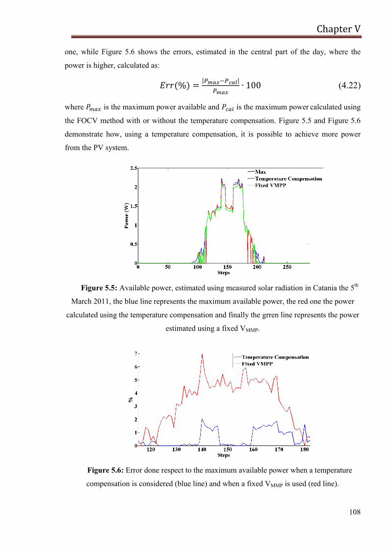
Chapter V

108

one, while Figure 5.6 shows the errors, estimated in the central part of the day, where the

power is higher, calculated as:

(4.22)

where is the maximum power available and is the maximum power calculated using

the FOCV method with or without the temperature compensation. Figure 5.5 and Figure 5.6

demonstrate how, using a temperature compensation, it is possible to achieve more power

from the PV system.

Figure 5.5: Available power, estimated using measured solar radiation in Catania the 5th

March 2011, the blue line represents the maximum available power, the red one the power

calculated using the temperature compensation and finally the grren line represents the power

estimated using a fixed VMMP.

Figure 5.6: Error done respect to the maximum available power when a temperature

compensation is considered (blue line) and when a fixed VMMP is used (red line).

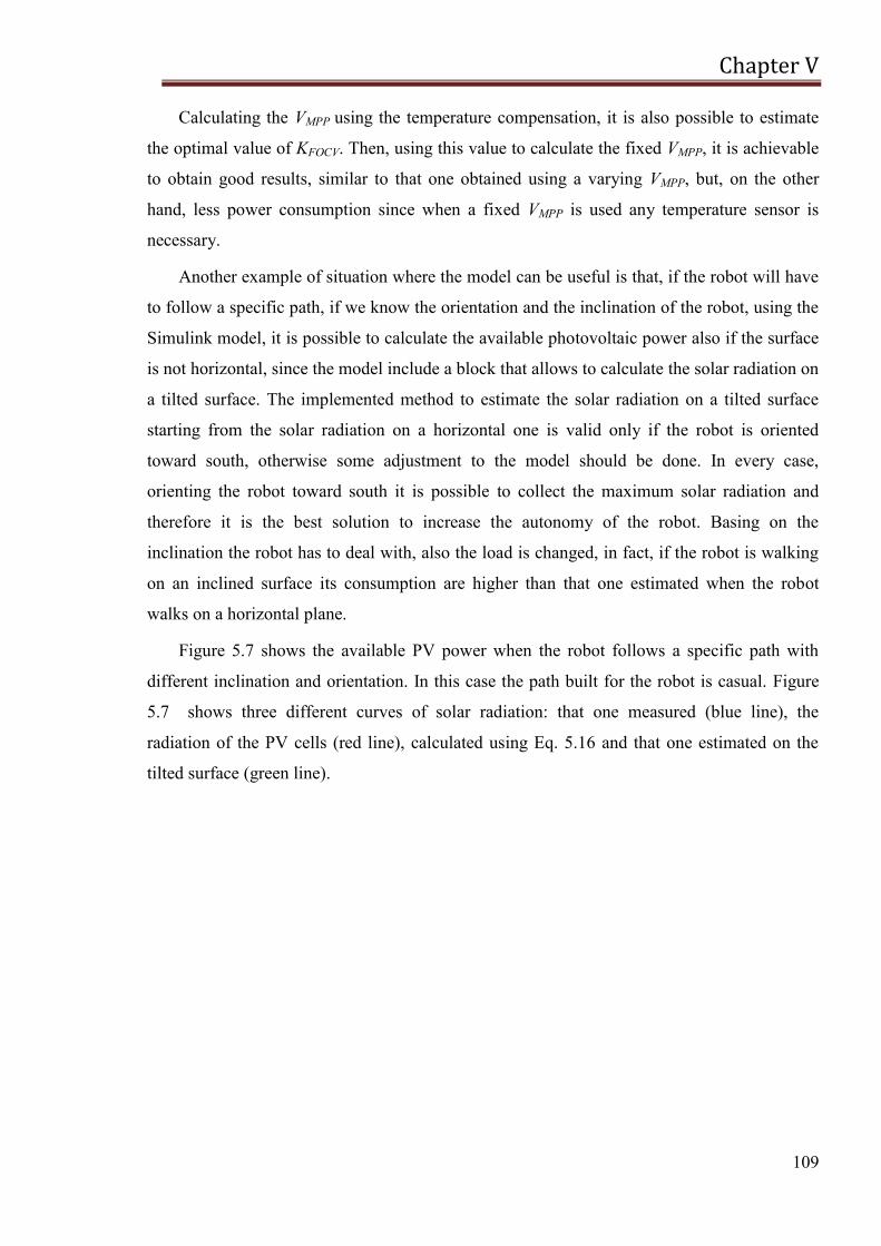
Chapter V

109

Calculating the VMPP using the temperature compensation, it is also possible to estimate

the optimal value of KFOCV. Then, using this value to calculate the fixed VMPP, it is achievable

to obtain good results, similar to that one obtained using a varying VMPP, but, on the other

hand, less power consumption since when a fixed VMPP is used any temperature sensor is

necessary.

Another example of situation where the model can be useful is that, if the robot will have

to follow a specific path, if we know the orientation and the inclination of the robot, using the

Simulink model, it is possible to calculate the available photovoltaic power also if the surface

is not horizontal, since the model include a block that allows to calculate the solar radiation on

a tilted surface. The implemented method to estimate the solar radiation on a tilted surface

starting from the solar radiation on a horizontal one is valid only if the robot is oriented

toward south, otherwise some adjustment to the model should be done. In every case,

orienting the robot toward south it is possible to collect the maximum solar radiation and

therefore it is the best solution to increase the autonomy of the robot. Basing on the

inclination the robot has to deal with, also the load is changed, in fact, if the robot is walking

on an inclined surface its consumption are higher than that one estimated when the robot

walks on a horizontal plane.

Figure 5.7 shows the available PV power when the robot follows a specific path with

different inclination and orientation. In this case the path built for the robot is casual. Figure

5.7 shows three different curves of solar radiation: that one measured (blue line), the

radiation of the PV cells (red line), calculated using Eq. 5.16 and that one estimated on the

tilted surface (green line).

Chapter V

110

Figure 5.7: Solar radiation available in Catania (latitude 37°34‘ N, longitude 15° 10‘ E,

Italy) on the 5th

March 2011: measured values (blue line), radiation of the PV cells (red line),

radiation estimated on the tilted surface (green line).

As it is possible to note, there are some periods where the radiation on the tilted surface is

higher than the other one, that because in that period it is supposed that the robot inclination

and/or orientation is changed (the robot is oriented toward south).

In the model it is possible to use the measured solar radiation, or also to use the forecast

one. Therefore, it will be possible, forecasting the solar radiation, to know in advance the

energy that can be harvested from the environment and therefore to implement power saving

strategies for the robot or it is possible to calculate the optimal path that the robot should

follow to optimize the power.

Moreover, the Simulink model allows to estimate the State Of Charge of the batteries and

therefore to calculate the autonomy the robot will have. Figure 5.8 shows an example of the

path that the robot follows, considering both orientation (tilt angle) and orientation (azimuth

angle), assuming that it is always oriented toward south. As it is possible to note, the available

PV power is higher when the robot walk on a tilted surface, because the inclination allows to

increase the power production of the cells, but on the other hand, the power needed for the

load is higher. The power taken from the battery is the result of the difference between the

available PV power and the power needed for the load.

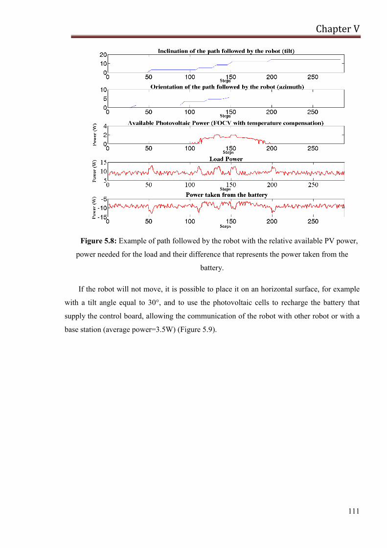
Chapter V

111

Figure 5.8: Example of path followed by the robot with the relative available PV power,

power needed for the load and their difference that represents the power taken from the

battery.

If the robot will not move, it is possible to place it on an horizontal surface, for example

with a tilt angle equal to 30°, and to use the photovoltaic cells to recharge the battery that

supply the control board, allowing the communication of the robot with other robot or with a

base station (average power=3.5W) (Figure 5.9).

Chapter V

112

Figure 5.9: Powers (available PV power, power of the load and that one taken from the

battery) when the load is represented by the control board with activated sensors.

Summary and Conclusions

113

Summary and Conclusions

In this thesis, the theoretical and experimental development of micro and mini systems

for the photovoltaic production and the energy storage has been presented.

First of all, a preliminary analysis of the feasibility of a photovoltaic system with batteries

to supply a mobile robot has been discussed. By analyzing both the power drawn by the robot

during the movement at various speed rates and the efficiency of the most used PV cell

technologies, it is clear that the PV system can supply only the control and wireless

transmission systems. Anyhow, using PV panels it will be possible to maintain the

communication of the robot with other robots, a charged station or the supervisor also if

batteries are discharged.

In the PV system analyzed in this thesis, a very efficient charging system is an essential

requisite, since the amount of area that can be used to place the PV cells is very limited and

therefore few solar cells are employed. To this aim, a novel photovoltaic charge regulator for

mobile applications, which uses the Fractional Open-Circuit Voltage MPPT method, has been

proposed. The purpose of the implemented MPPT algorithm was to optimize the efficiency of

the harvesting process, minimizing the complexity and therefore the power consumption. The

experiments allow to compare the system when any MPPT algorithms is used and when the

FOCV method is implemented. They demonstrate that the use of the MPPT technique allows

to increase the efficiency of the PV system.

Since a mobile robot is a structure in continuous movement, additional analysis in

transitory conditions, due to the variability of the solar exposure, must be done. To this aim, it

is necessary to evaluate the global solar radiation on a tilted surface. Global solar radiation

incident on a tilted plane is composed by three components: beam radiation, diffuse radiation

and reflected radiation from the ground. A simple method, based on the beam radiation tilt

factor, has been used for estimating beam solar radiation incident on tilted surfaces, while an

isotropic model has been used for estimating reflected component. On the contrary, different

models can be used to evaluate the diffuse radiation component; in this paper the Klucher and

Perez models have been implemented. These models need to split the global solar radiation on

a horizontal surface into beam and diffuse components, to do this a model, called CLIMED2,

developed by De Miguel et al, has been used. Moreover, a neural network that allows to

Summary and Conclusions

114

evaluate the global solar radiation on a tilted surface directly from the horizontal global solar

radiation has been developed.

It should be very useful to know in advance the available solar radiation, since the

knowledge of the solar radiation allows to calculate the available photovoltaic power and

therefore to implement power saving strategies for the robot. For this reason, predicted solar

radiation on a horizontal surface, given us by weather forecast provider, have been taken into

consideration and analyzed. First of all, the accuracy of these data has been evaluated, using

the normalized Root Mean Square Error (nRMSE) as mean measure, then an algorithm that

allows to classify days thought four value of percentages: variable, cloudy, slightly cloudy or

clear, has been developed. The aim was to develop a neural network that allows to

approximate the nRMSE starting from the value of these percentages. Analyzing the nRMSE

and the correspondent four values of percentages, it is possible to note that the error done on

the forecast data is lower if the slightly cloudy or clear percentages are higher that the variable

or cloudy ones. Moreover, forecasting solar radiation using hourly data causes the lost of the

dynamic of the solar radiation curve and therefore the classification appears to be different

from the real one, thus sub-hourly data have been used (10 minutes). Our target was to

predict the nRMSE knowing the four value of percentages calculated using the forecast solar

radiation, through the implemented neural network. To evaluate the effectiveness of the

approximation, the mean square error has been evaluated, it was equal to 0.0640 when the

input of the neural network were the four percentages calculated starting from measured data,

while it was equal to 0.9604 when the inputs were the percentages calculated using forecast

data. Therefore, results can be considered satisfying.

In contrast with the previous works about models that allow to calculate the solar

radiation on an inclined surface starting from that one on the horizontal surface, that use

hourly data, basing on the evaluation done about the sampling time in the estimation of the

classification of days, in this work sub-hourly data have been used. To test the models and the

neural network, data collected in a year in a meteorological station of Ajaccio-Vignola have

been used, considering two inclination angle (45° and 60°). To evaluate the effectiveness of

the approximation done using the models and the neural network in the evaluation of the

radiation on an inclined plane, three statistical parameters have been evaluated: the Relative

Mean Square Error, the Relative Root Mean Square Error and the Correlation Coefficient,

obtaining results that can be considered satisfying. Using data measured and estimated every

10 minutes it is possible to obtain better results. Moreover, the Klucher and the Perez models

have been applied from sunrise to sunset times on the inclined surface, while the diffuse

Summary and Conclusions

115

component on the tilted surface has been set equal to that one on the horizontal surface from

sunrise time on horizontal surface to sunrise time on inclined one and from sunset time on

horizontal surface to sunset time on inclined one, demonstrating that in this way it is possible

to obtain a more accurate approximation of the measured radiation on tilted surfaces.

The PV system includes a solar array, batteries, regulator and load. In order to simulate

the behaviour of the whole system, a Simulink model in Matlab environment has been used.

This model has the measured temperature and solar radiation as inputs, but the forecast values

can also be used. Moreover, it allows to consider the solar radiation on a tilted surface if the

robot walks on an irregular environment. Thanks to the implementation of the MPPT charge

regulator, it is also possible to evaluate the performance of different MPPT algorithms and to

estimate the available photovoltaic power and that one needed for the load. Therefore this

model can be considered as a very useful tool to estimate the performance of the whole

photovoltaic system and can be used for the optimal sizing.

Appendix A

116

APPENDIX A

Environmental Characteristics

From the very beginning of its history humankind realized that a good use of solar energy

is in humankind‘s benefit. Despite this, only recently, during the last 40 years, has solar

energy been harnessed with specialized equipment and used as an alternative source of

energy, mainly because it is free and does not harm the environment [1].

Solar-based conversion systems, in fact, are typical examples of renewable and

sustainable energy technologies which generate energy without emitting pollutants and

requiring no fuel [151].

6.1. Incident radiation and its components

Irradiance is the rate at which radiant energy is incident on a surface per unit area of

surface. The total irradiance incident on a surface has three components:

Beam radiation, : The part of solar radiation that reaches the earth without any

change in direction. It is also known as direct radiation.

Diffuse radiation, : The solar radiation received by the earth after its direction gets

changed because of scattering in the atmosphere is known as diffuse radiation. On a

horizontal surface it can be measured using a pyranometer with a tracking device that

shields the beam irradiance or if the total irradiance is known, from Equation 1:

(6.1)

Ground-Reflected radiation, :radiation that results from reflection of the global

solar radiation by the surface of the Earth and by any surface intercepting that

radiation

Total solar radiation, : The sum of the beam and the diffuse components of solar

radiation is called total solar radiation.

Appendix A

117

6.2. Solar trajectory

In solar energy applications, the knowledge of the geometrical parameters of the solar

trajectory is necessary to calculate solar radiation falling on a surface, the solar heat gain, the

proper orientation of solar collectors, the placement of collectors to avoid shading and many

more factors.

The geometric relationship between a plane of any particular orientation relative to the

earth at any time (whether that plane is fixed or moving to the earth) and the incoming beam

insolation, that is the position of the sun relative to that plane, can be described in terms of

several angles [152]: latitude, declination, surface slope, surface azimuth angle, hour angle

and incidence angle. In the following paragraphs they will be defined.

Each location on the Earth can be specified by a set of numbers. The coordinates are

often chosen such that one of the numbers represent vertical position, and two or three of the

numbers represent horizontal position. A common choice of coordinates is latitude (Lat),

longitude (Long) and elevation (lev) [153].

The geographic latitude of a point on the Earth's surface is the angle between the

equatorial plane and a line that passes through that point and is normal to the surface of a

reference ellipsoid which approximates the shape of the Earth. This line passes a few

kilometers away from the center of the Earth except at the poles and the equator where it

passes through Earth's center. It is measured from the equator, with positive values going

north and negative values going south. While, the longitude of a point on the Earth's surface is

the angle east or west from a reference meridian to another meridian that passes through that

point. All meridians are halves of great ellipses, which converge at the north and south poles.

It is measured from the Prime Meridian (which is the longitude that runs through Greenwich,

England), with positive values going east and negative values going west.

Appendix A

118

Figure 22: The parallels of latitude and meridians of longitude.

The earth makes one rotation about its axis every 24h and completes a revolution about

the sun in a period of approximately 365.25 days. This revolution is not circular but follows

an ellipse with the sun at one of the foci, as shown in Figure 6.2 [1].

Figure 6.2: Annual motion of the earth about the sun.

The sun‘s position in the sky changes day to day and from hour to hour. It is common

knowledge that the sun is higher in the sky during the summer than during the winter. The

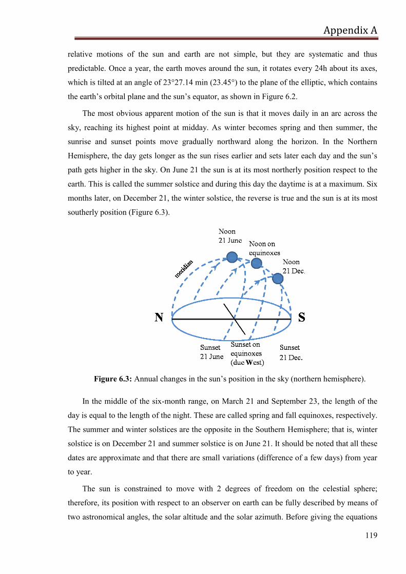
Appendix A

119

relative motions of the sun and earth are not simple, but they are systematic and thus

predictable. Once a year, the earth moves around the sun, it rotates every 24h about its axes,

which is tilted at an angle of 23°27.14 min (23.45°) to the plane of the elliptic, which contains

the earth‘s orbital plane and the sun‘s equator, as shown in Figure 6.2.

The most obvious apparent motion of the sun is that it moves daily in an arc across the

sky, reaching its highest point at midday. As winter becomes spring and then summer, the

sunrise and sunset points move gradually northward along the horizon. In the Northern

Hemisphere, the day gets longer as the sun rises earlier and sets later each day and the sun‘s

path gets higher in the sky. On June 21 the sun is at its most northerly position respect to the

earth. This is called the summer solstice and during this day the daytime is at a maximum. Six

months later, on December 21, the winter solstice, the reverse is true and the sun is at its most

southerly position (Figure 6.3).

Figure 6.3: Annual changes in the sun‘s position in the sky (northern hemisphere).

In the middle of the six-month range, on March 21 and September 23, the length of the

day is equal to the length of the night. These are called spring and fall equinoxes, respectively.

The summer and winter solstices are the opposite in the Southern Hemisphere; that is, winter

solstice is on December 21 and summer solstice is on June 21. It should be noted that all these

dates are approximate and that there are small variations (difference of a few days) from year

to year.

The sun is constrained to move with 2 degrees of freedom on the celestial sphere;

therefore, its position with respect to an observer on earth can be fully described by means of

two astronomical angles, the solar altitude and the solar azimuth. Before giving the equations

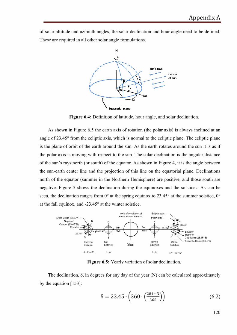
Appendix A

120

of solar altitude and azimuth angles, the solar declination and hour angle need to be defined.

These are required in all other solar angle formulations.

Figure 6.4: Definition of latitude, hour angle, and solar declination.

As shown in Figure 6.5 the earth axis of rotation (the polar axis) is always inclined at an

angle of 23.45° from the ecliptic axis, which is normal to the ecliptic plane. The ecliptic plane

is the plane of orbit of the earth around the sun. As the earth rotates around the sun it is as if

the polar axis is moving with respect to the sun. The solar declination is the angular distance

of the sun‘s rays north (or south) of the equator. As shown in Figure 4, it is the angle between

the sun-earth center line and the projection of this line on the equatorial plane. Declinations

north of the equator (summer in the Northern Hemisphere) are positive, and those south are

negative. Figure 5 shows the declination during the equinoxes and the solstices. As can be

seen, the declination ranges from 0° at the spring equinox to 23.45° at the summer solstice, 0°

at the fall equinox, and -23.45° at the winter solstice.

Figure 6.5: Yearly variation of solar declination.

The declination, , in degrees for any day of the year (N) can be calculated approximately

by the equation [153]:

(6.2)

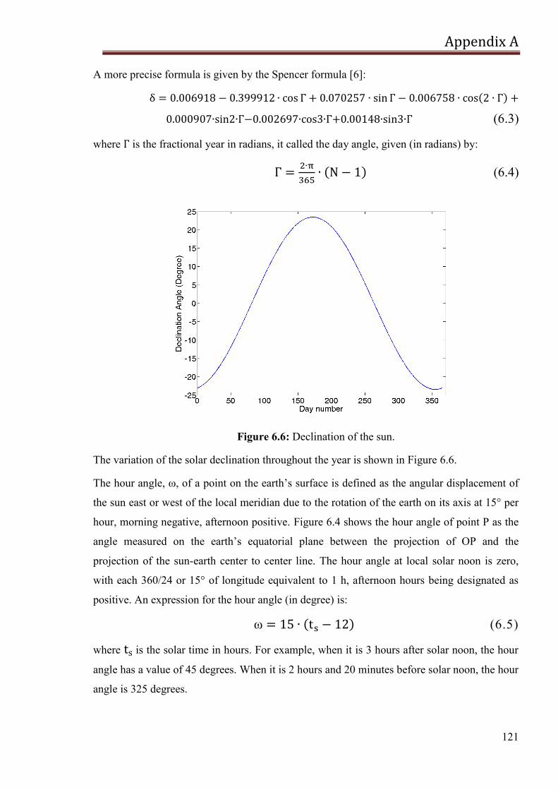
Appendix A

121

A more precise formula is given by the Spencer formula [6]:

sin 0.002697 cos sin (6.3)

where is the fractional year in radians, it called the day angle, given (in radians) by:

(6.4)

Figure 6.6: Declination of the sun.

The variation of the solar declination throughout the year is shown in Figure 6.6.

The hour angle, ω, of a point on the earth‘s surface is defined as the angular displacement of

the sun east or west of the local meridian due to the rotation of the earth on its axis at 15° per

hour, morning negative, afternoon positive. Figure 6.4 shows the hour angle of point P as the

angle measured on the earth‘s equatorial plane between the projection of OP and the

projection of the sun-earth center to center line. The hour angle at local solar noon is zero,

with each 360/24 or 15° of longitude equivalent to 1 h, afternoon hours being designated as

positive. An expression for the hour angle (in degree) is:

ω (6.5)

where is the solar time in hours. For example, when it is 3 hours after solar noon, the hour

angle has a value of 45 degrees. When it is 2 hours and 20 minutes before solar noon, the hour

angle is 325 degrees.

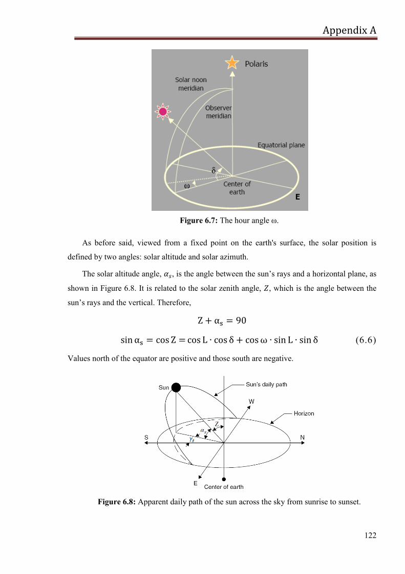
Appendix A

122

Figure 6.7: The hour angle ω.

As before said, viewed from a fixed point on the earth's surface, the solar position is

defined by two angles: solar altitude and solar azimuth.

The solar altitude angle, , is the angle between the sun‘s rays and a horizontal plane, as

shown in Figure 6.8. It is related to the solar zenith angle, , which is the angle between the

sun‘s rays and the vertical. Therefore,

(6.6)

Values north of the equator are positive and those south are negative.

Figure 6.8: Apparent daily path of the sun across the sky from sunrise to sunset.

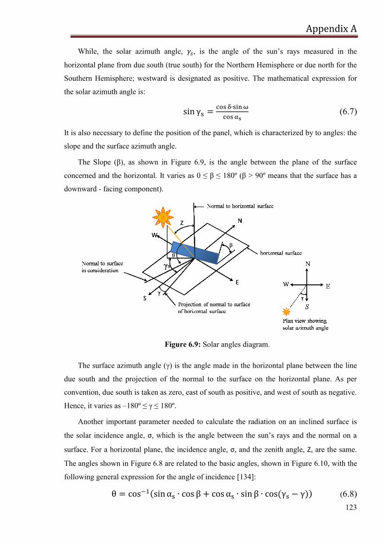
Appendix A

123

While, the solar azimuth angle, , is the angle of the sun‘s rays measured in the

horizontal plane from due south (true south) for the Northern Hemisphere or due north for the

Southern Hemisphere; westward is designated as positive. The mathematical expression for

the solar azimuth angle is:

(6.7)

It is also necessary to define the position of the panel, which is characterized by to angles: the

slope and the surface azimuth angle.

The Slope (β), as shown in Figure 6.9, is the angle between the plane of the surface

concerned and the horizontal. It varies as 0 ≤ β ≤ 180º (β > 90º means that the surface has a

downward - facing component).

Figure 6.9: Solar angles diagram.

The surface azimuth angle (γ) is the angle made in the horizontal plane between the line

due south and the projection of the normal to the surface on the horizontal plane. As per

convention, due south is taken as zero, east of south as positive, and west of south as negative.

Hence, it varies as –180º ≤ γ ≤ 180º.

Another important parameter needed to calculate the radiation on an inclined surface is

the solar incidence angle, σ, which is the angle between the sun‘s rays and the normal on a

surface. For a horizontal plane, the incidence angle, σ, and the zenith angle, Z, are the same.

The angles shown in Figure 6.8 are related to the basic angles, shown in Figure 6.10, with the

following general expression for the angle of incidence [134]:

(6.8)

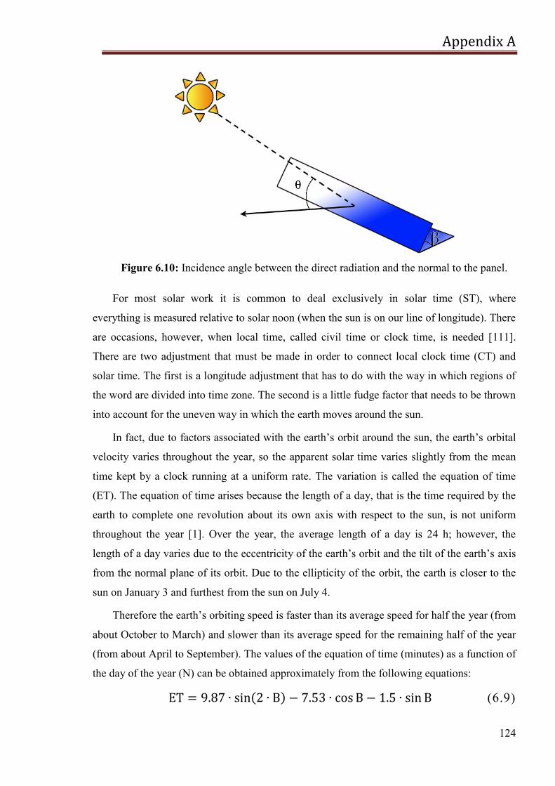
Appendix A

124

Figure 6.10: Incidence angle between the direct radiation and the normal to the panel.

For most solar work it is common to deal exclusively in solar time (ST), where

everything is measured relative to solar noon (when the sun is on our line of longitude). There

are occasions, however, when local time, called civil time or clock time, is needed [111].

There are two adjustment that must be made in order to connect local clock time (CT) and

solar time. The first is a longitude adjustment that has to do with the way in which regions of

the word are divided into time zone. The second is a little fudge factor that needs to be thrown

into account for the uneven way in which the earth moves around the sun.

In fact, due to factors associated with the earth‘s orbit around the sun, the earth‘s orbital

velocity varies throughout the year, so the apparent solar time varies slightly from the mean

time kept by a clock running at a uniform rate. The variation is called the equation of time

(ET). The equation of time arises because the length of a day, that is the time required by the

earth to complete one revolution about its own axis with respect to the sun, is not uniform

throughout the year [1]. Over the year, the average length of a day is 24 h; however, the

length of a day varies due to the eccentricity of the earth‘s orbit and the tilt of the earth‘s axis

from the normal plane of its orbit. Due to the ellipticity of the orbit, the earth is closer to the

sun on January 3 and furthest from the sun on July 4.

Therefore the earth‘s orbiting speed is faster than its average speed for half the year (from

about October to March) and slower than its average speed for the remaining half of the year

(from about April to September). The values of the equation of time (minutes) as a function of

the day of the year (N) can be obtained approximately from the following equations:

(6.9)

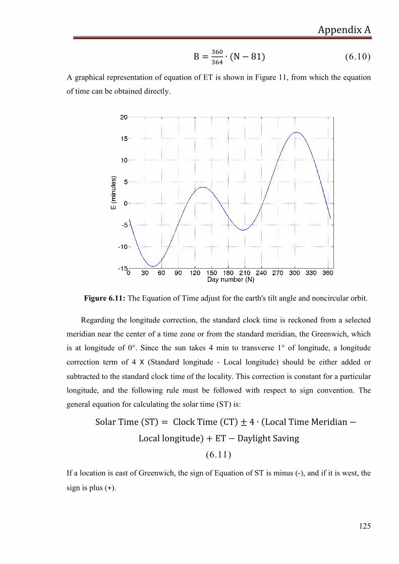
Appendix A

125

(6.10)

A graphical representation of equation of ET is shown in Figure 11, from which the equation

of time can be obtained directly.

Figure 6.11: The Equation of Time adjust for the earth's tilt angle and noncircular orbit.

Regarding the longitude correction, the standard clock time is reckoned from a selected

meridian near the center of a time zone or from the standard meridian, the Greenwich, which

is at longitude of 0°. Since the sun takes 4 min to transverse 1° of longitude, a longitude

correction term of 4 X (Standard longitude - Local longitude) should be either added or

subtracted to the standard clock time of the locality. This correction is constant for a particular

longitude, and the following rule must be followed with respect to sign convention. The

general equation for calculating the solar time (ST) is:

(6.11)

If a location is east of Greenwich, the sign of Equation of ST is minus (-), and if it is west, the

sign is plus (+).

Appendix A

126

Moreover, if a daylight saving time is used, this must be subtracted from the local

standard time. The term can be either 0 or 60 min and it depends on

whether daylight saving time is in operation (usually from end of March to end of October) or

not. This term is usually ignored from this equation and considered only if the estimation is

within the Daylight Saving period.

Basic information needed to estimate hourly values of solar irradiance is the position of

the sun in the sky and therefore the sunrise and sunset hours on the day. The astronomical day

begins and ends when the centre of the sun's disk is precisely on the (flat) horizon, ignoring

atmospheric refraction.

The value of the hour angles of sunrise (SR) and sunset (SS) on a horizontal surface at

the latitude of the site in question can be found from a simple observation: at sunrise and

sunset the altitude angle is zero, and therefore [112]:

(6.12)

Since the inverse cosine allows for both positive and negative values, it is necessary to use a

sign convention. Here SR is taken as positive at sunset. Since the hour angle at local solar

noon is 0°, with each 15° of longitude equivalent to 1 h, the sunrise and sunset time in hours

from local solar noon is then:

(6.13)

For surface sloped toward the equator in the northern hemisphere, that is for surface with γ=0,

the sunset hour angles for a tilted surface is given by [112]:

(6.14)

While for surface in the southern hemisphere sloped toward the equator, with γ=180, the

equation are [112]:

(6.15)

While, for a surface of any orientation, the sunrise and sunset hour angles can be calculated

using the following equation [1]:

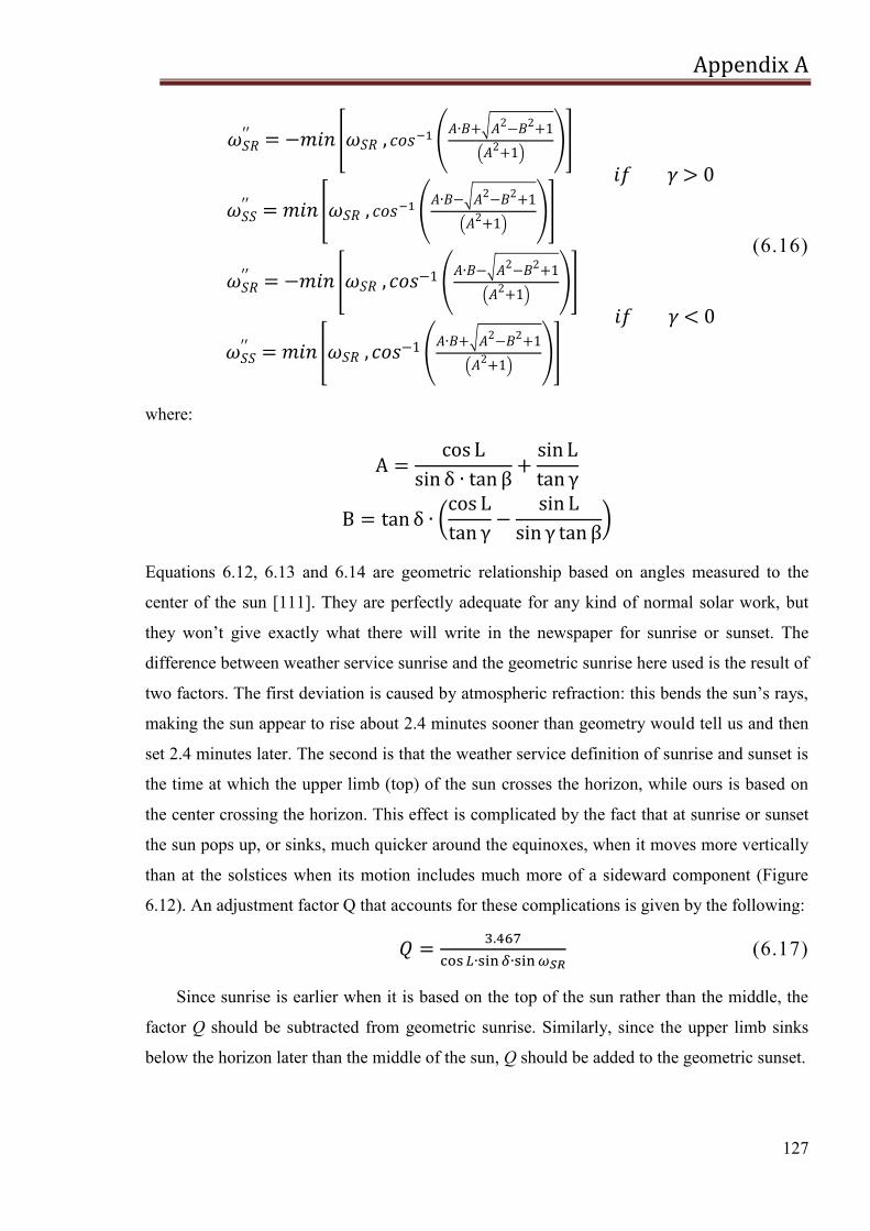
Appendix A

127

(6.16)

where:

Equations 6.12, 6.13 and 6.14 are geometric relationship based on angles measured to the

center of the sun [111]. They are perfectly adequate for any kind of normal solar work, but

they won‘t give exactly what there will write in the newspaper for sunrise or sunset. The

difference between weather service sunrise and the geometric sunrise here used is the result of

two factors. The first deviation is caused by atmospheric refraction: this bends the sun‘s rays,

making the sun appear to rise about 2.4 minutes sooner than geometry would tell us and then

set 2.4 minutes later. The second is that the weather service definition of sunrise and sunset is

the time at which the upper limb (top) of the sun crosses the horizon, while ours is based on

the center crossing the horizon. This effect is complicated by the fact that at sunrise or sunset

the sun pops up, or sinks, much quicker around the equinoxes, when it moves more vertically

than at the solstices when its motion includes much more of a sideward component (Figure

6.12). An adjustment factor Q that accounts for these complications is given by the following:

(6.17)

Since sunrise is earlier when it is based on the top of the sun rather than the middle, the

factor Q should be subtracted from geometric sunrise. Similarly, since the upper limb sinks

below the horizon later than the middle of the sun, Q should be added to the geometric sunset.

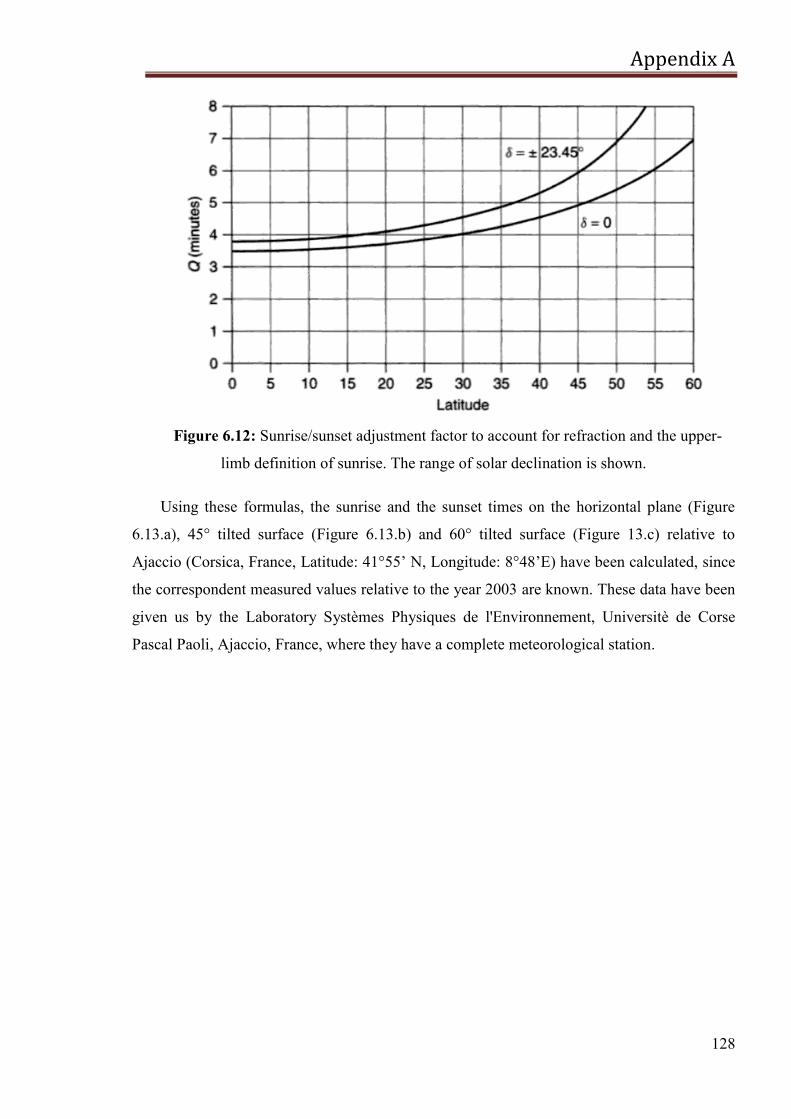
Appendix A

128

Figure 6.12: Sunrise/sunset adjustment factor to account for refraction and the upper-

limb definition of sunrise. The range of solar declination is shown.

Using these formulas, the sunrise and the sunset times on the horizontal plane (Figure

6.13.a), 45° tilted surface (Figure 6.13.b) and 60° tilted surface (Figure 13.c) relative to

Ajaccio (Corsica, France, Latitude: 41°55‘ N, Longitude: 8°48‘E) have been calculated, since

the correspondent measured values relative to the year 2003 are known. These data have been

given us by the Laboratory Systèmes Physiques de l'Environnement, Universitè de Corse

Pascal Paoli, Ajaccio, France, where they have a complete meteorological station.

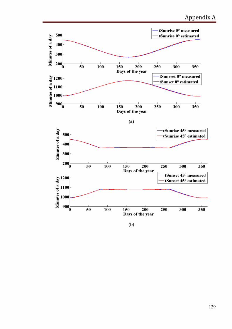
Appendix A

129

(a)

(b)

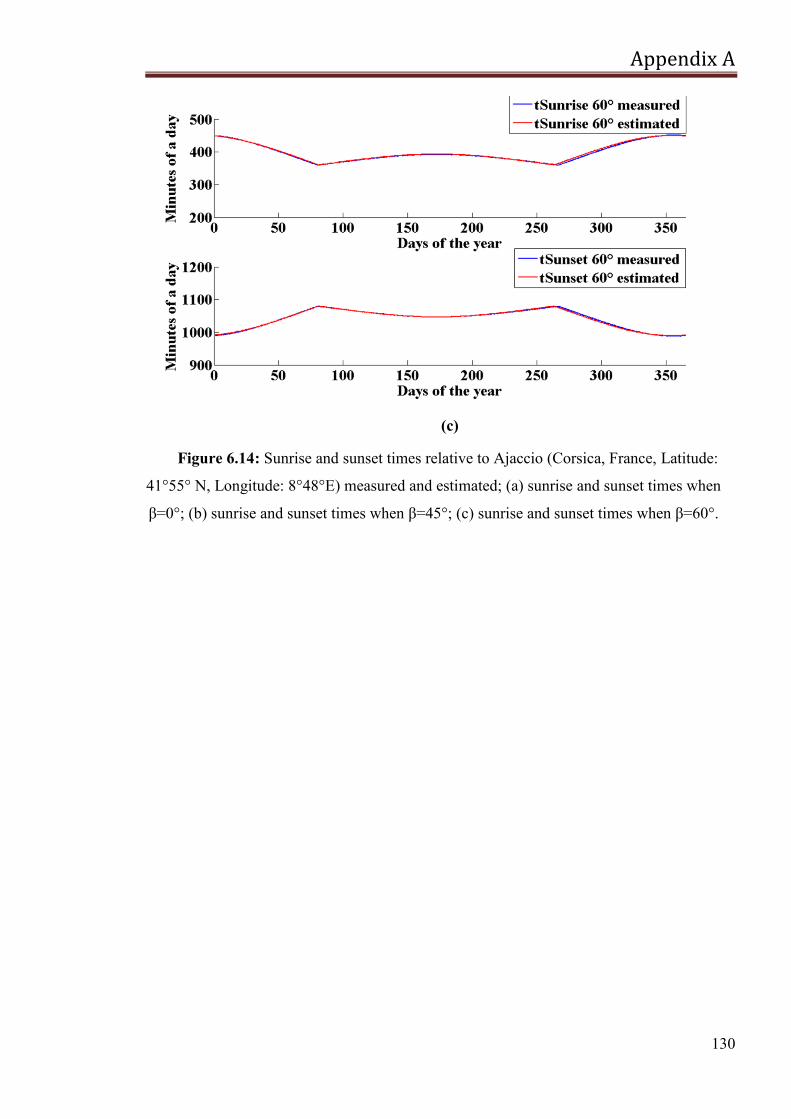
Appendix A

130

(c)

Figure 6.14: Sunrise and sunset times relative to Ajaccio (Corsica, France, Latitude:

41°55° N, Longitude: 8°48°E) measured and estimated; (a) sunrise and sunset times when

β=0°; (b) sunrise and sunset times when β=45°; (c) sunrise and sunset times when β=60°.

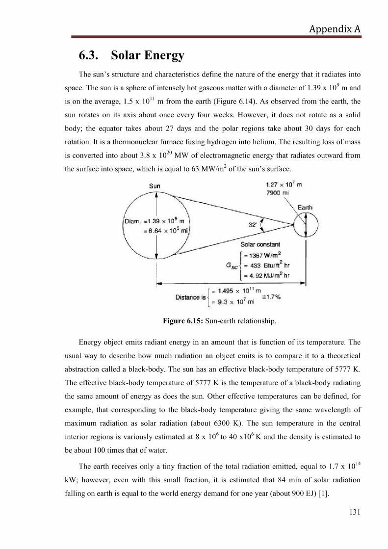
Appendix A

131

6.3. Solar Energy

The sun‘s structure and characteristics define the nature of the energy that it radiates into

space. The sun is a sphere of intensely hot gaseous matter with a diameter of 1.39 x 109 m and

is on the average, 1.5 x 1011

m from the earth (Figure 6.14). As observed from the earth, the

sun rotates on its axis about once every four weeks. However, it does not rotate as a solid

body; the equator takes about 27 days and the polar regions take about 30 days for each

rotation. It is a thermonuclear furnace fusing hydrogen into helium. The resulting loss of mass

is converted into about 3.8 x 1020

MW of electromagnetic energy that radiates outward from

the surface into space, which is equal to 63 MW/m2 of the sun‘s surface.

Figure 6.15: Sun-earth relationship.

Energy object emits radiant energy in an amount that is function of its temperature. The

usual way to describe how much radiation an object emits is to compare it to a theoretical

abstraction called a black-body. The sun has an effective black-body temperature of 5777 K.

The effective black-body temperature of 5777 K is the temperature of a black-body radiating

the same amount of energy as does the sun. Other effective temperatures can be defined, for

example, that corresponding to the black-body temperature giving the same wavelength of

maximum radiation as solar radiation (about 6300 K). The sun temperature in the central

interior regions is variously estimated at 8 x 106

to 40 x106

K and the density is estimated to

be about 100 times that of water.

The earth receives only a tiny fraction of the total radiation emitted, equal to 1.7 x 1014

kW; however, even with this small fraction, it is estimated that 84 min of solar radiation

falling on earth is equal to the world energy demand for one year (about 900 EJ) [1].

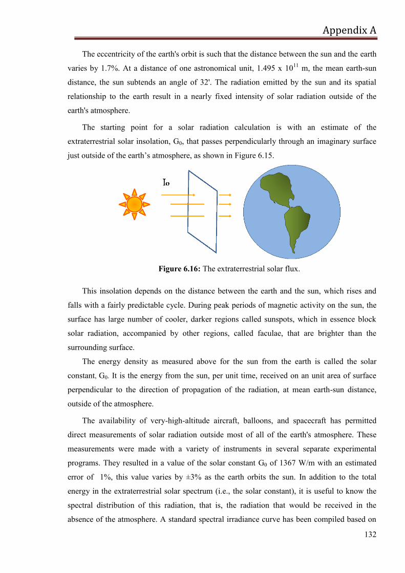
Appendix A

132

The eccentricity of the earth's orbit is such that the distance between the sun and the earth

varies by 1.7%. At a distance of one astronomical unit, 1.495 x 1011

m, the mean earth-sun

distance, the sun subtends an angle of 32'. The radiation emitted by the sun and its spatial

relationship to the earth result in a nearly fixed intensity of solar radiation outside of the

earth's atmosphere.

The starting point for a solar radiation calculation is with an estimate of the

extraterrestrial solar insolation, G0, that passes perpendicularly through an imaginary surface

just outside of the earth‘s atmosphere, as shown in Figure 6.15.

Figure 6.16: The extraterrestrial solar flux.

This insolation depends on the distance between the earth and the sun, which rises and

falls with a fairly predictable cycle. During peak periods of magnetic activity on the sun, the

surface has large number of cooler, darker regions called sunspots, which in essence block

solar radiation, accompanied by other regions, called faculae, that are brighter than the

surrounding surface.

The energy density as measured above for the sun from the earth is called the solar

constant, G0. It is the energy from the sun, per unit time, received on an unit area of surface

perpendicular to the direction of propagation of the radiation, at mean earth-sun distance,

outside of the atmosphere.

The availability of very-high-altitude aircraft, balloons, and spacecraft has permitted

direct measurements of solar radiation outside most of all of the earth's atmosphere. These

measurements were made with a variety of instruments in several separate experimental

programs. They resulted in a value of the solar constant G0 of 1367 W/m with an estimated

error of 1%, this value varies by ±3% as the earth orbits the sun. In addition to the total

energy in the extraterrestrial solar spectrum (i.e., the solar constant), it is useful to know the

spectral distribution of this radiation, that is, the radiation that would be received in the

absence of the atmosphere. A standard spectral irradiance curve has been compiled based on

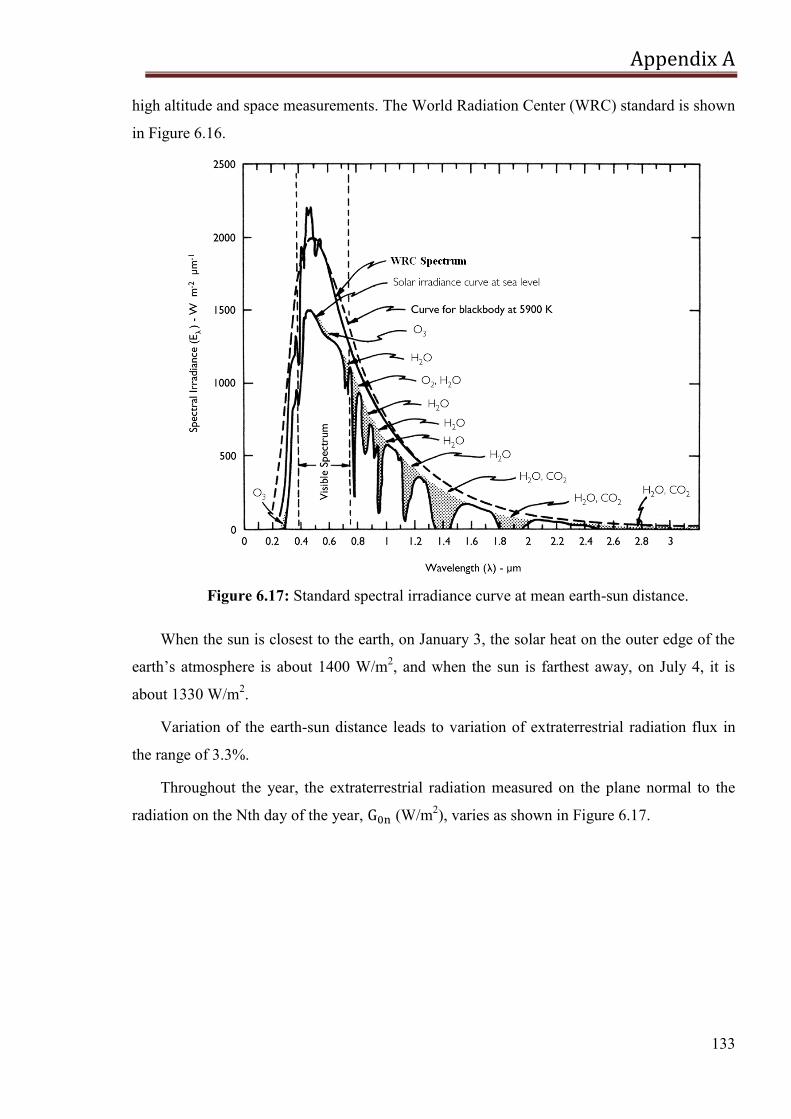
Appendix A

133

high altitude and space measurements. The World Radiation Center (WRC) standard is shown

in Figure 6.16.

Figure 6.17: Standard spectral irradiance curve at mean earth-sun distance.

When the sun is closest to the earth, on January 3, the solar heat on the outer edge of the

earth‘s atmosphere is about 1400 W/m2, and when the sun is farthest away, on July 4, it is

about 1330 W/m2.

Variation of the earth-sun distance leads to variation of extraterrestrial radiation flux in

the range of 3.3%.

Throughout the year, the extraterrestrial radiation measured on the plane normal to the

radiation on the Nth day of the year, (W/m2), varies as shown in Figure 6.17.

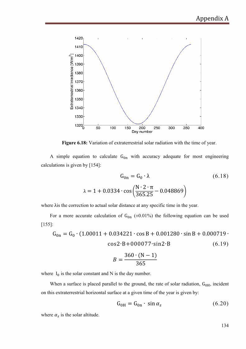
Appendix A

134

Figure 6.18: Variation of extraterrestrial solar radiation with the time of year.

A simple equation to calculate with accuracy adequate for most engineering

calculations is given by [154]:

(6.18)

where is the correction to actual solar distance at any specific time in the year.

For a more accurate calculation of (±0.01%) the following equation can be used

[155]:

cos sin (6.19)

where is the solar constant and N is the day number.

When a surface is placed parallel to the ground, the rate of solar radiation, , incident

on this extraterrestrial horizontal surface at a given time of the year is given by:

(6.20)

where is the solar altitude.

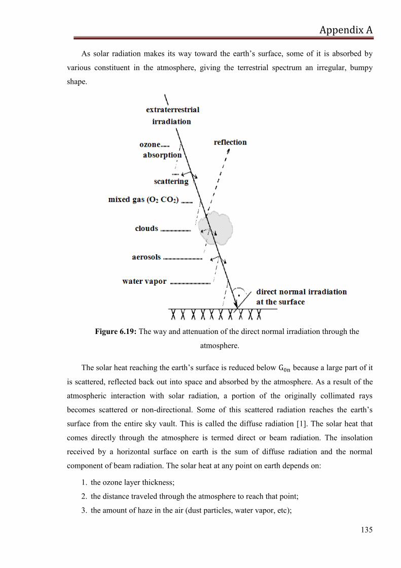
Appendix A

135

As solar radiation makes its way toward the earth‘s surface, some of it is absorbed by

various constituent in the atmosphere, giving the terrestrial spectrum an irregular, bumpy

shape.

Figure 6.19: The way and attenuation of the direct normal irradiation through the

atmosphere.

The solar heat reaching the earth‘s surface is reduced below because a large part of it

is scattered, reflected back out into space and absorbed by the atmosphere. As a result of the

atmospheric interaction with solar radiation, a portion of the originally collimated rays

becomes scattered or non-directional. Some of this scattered radiation reaches the earth‘s

surface from the entire sky vault. This is called the diffuse radiation [1]. The solar heat that

comes directly through the atmosphere is termed direct or beam radiation. The insolation

received by a horizontal surface on earth is the sum of diffuse radiation and the normal

component of beam radiation. The solar heat at any point on earth depends on:

1. the ozone layer thickness;

2. the distance traveled through the atmosphere to reach that point;

3. the amount of haze in the air (dust particles, water vapor, etc);

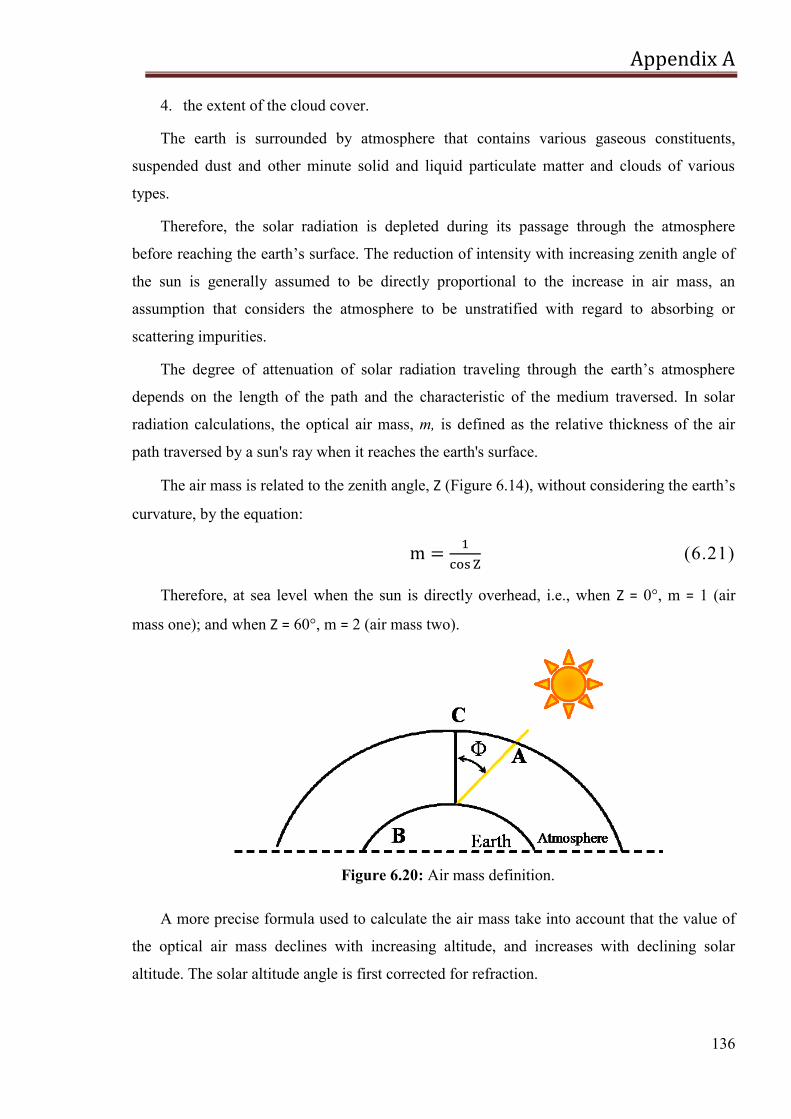
Appendix A

136

4. the extent of the cloud cover.

The earth is surrounded by atmosphere that contains various gaseous constituents,

suspended dust and other minute solid and liquid particulate matter and clouds of various

types.

Therefore, the solar radiation is depleted during its passage through the atmosphere

before reaching the earth‘s surface. The reduction of intensity with increasing zenith angle of

the sun is generally assumed to be directly proportional to the increase in air mass, an

assumption that considers the atmosphere to be unstratified with regard to absorbing or

scattering impurities.

The degree of attenuation of solar radiation traveling through the earth‘s atmosphere

depends on the length of the path and the characteristic of the medium traversed. In solar

radiation calculations, the optical air mass, m, is defined as the relative thickness of the air

path traversed by a sun's ray when it reaches the earth's surface.

The air mass is related to the zenith angle, Z (Figure 6.14), without considering the earth‘s

curvature, by the equation:

(6.21)

Therefore, at sea level when the sun is directly overhead, i.e., when Z = 0°, m = 1 (air

mass one); and when Z = 60°, m = 2 (air mass two).

Figure 6.20: Air mass definition.

A more precise formula used to calculate the air mass take into account that the value of

the optical air mass declines with increasing altitude, and increases with declining solar

altitude. The solar altitude angle is first corrected for refraction.

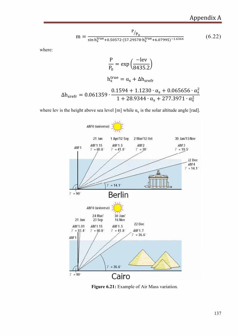
Appendix A

137

(6.22)

where:

where lev is the height above sea level [m] while is the solar altitude angle [rad].

Figure 6.21: Example of Air Mass variation.

Bibliography

138

Bibliography

[1] Soteris A. Kalogirou; ―Solar Energy Engineering: Processes and System‖,

Elsevier, 2009.

[2] S. Kalogirou; ―Solar thermal collectors and applications‖, Prog. Energ. Combust.

Sci, Vol. 30, issue 3, pages 231–295, 2004.

[3] Anca D. Hansen, Poul Sørensen, Lars H. Hansen and Henrik Bindner; ―Models

for a Stand-Alone PV System‖, Risø National Laboratory, Roskilde, December 2000.

[4] J.A. Ramos Hernanz, J.J. Campayo Martín, I. Zamora Belver, J. Larrañaga

Lesaka, E. Zulueta Guerrero and E.P. Pérez; ―Modelling of Photovoltaic Module‖,

International Conference on Renewable Energies and Power Quality (ICREPQ‘10), Granada,

Spain, 23-25 March, 2010.

[5] Gilbert M. Masters; ―Renewable and efficient electric power systems‖, John

Wiley & Sons, 2004.

[6] Practical Handbook of Photovoltaics: From Fundamentals to Applications

Publisher, Elsevier

[7] F.M. Gonzàlez-Longatt; ―Model of Photovoltaic Module in Matlab‖, II

CIBELEC, Puerto La Cruz, Venezuela, December 2005.

[8] D. P. Kaundinya, P. Balachandra and N.H. Ravindranath; "Grid-connected

versus stand-alone energy systems for decentralized power—A review of literature",

Renewable and Sustainable Energy Reviews, vol. 13, issue 8, pages 2041-2050, October

2009.

[9] Planning Commission Report. Integrated Energy Policy. Technical report.

Government of India; 2006.

[10] R. Hiremath, S. Shikha and N. Ravindranath; ―Decentralized energy planning;

modeling and application-a review‖, Renewable and Sustainable Energy Reviews, vol. 11,

issue 5, pages 729–52, 2007.

[11] WADE (World Alliance for Decentralized Energy). World Survey of

Decentralized Energy-2005. Survey Paper; 2005.

[12] G. Dzimano; ―Modeling of Photovoltaic Systems‖, Doctoral thesis, the Ohio

State University, 2008.

Bibliography

139

[13] L. Kazmerski; ―Photovoltaics: a review of cell and module technologies‖,

Renewable and Sustainable Energy Rev., vol. 1 (1–2), pages 71–170, 1997.

[14] J. Nelson; ―Organic photovoltaic films‖, Curr. Opin. Solid State Mater. Sci.,

vol. 6, issue 1, pages 87–95, 2002.

[15] D. Brunelli, D. Dondi, A. Bertacchini, L. Larcher, P. Pavan and L. Benini;

―Photovoltaic scavenging systems: Modeling and optimization‖, Microelectronics Journal, vol

40, pages1337–1344, 2009.

[16] X. Jiang, J. Polastre, and D. Culler; "Perpetual environmentally powered sensor

networks", Proceedings of the 4th

international symposium on Information processing in

sensor networks}, Los Angeles, California, 2005.

[17] P. Dutta, J. Hui, J. Jeong, S. Kim, C. Sharp, J. Taneja, G. Tolle, K. Whitehouse

and D. Culler; "Trio: Enabling sustainable and scalable outdoor wireless sensor network

deployments" Proceedings of the 5th

international conference on Information processing in

sensor networks, pages 407 - 415, Nashville, Tennessee, USA, 2006.

[18] F. Simjee and P. H. Chou; "Everlast: Long-life, supercapacitor-operated

wireless sensor node", Proceedings of the 3rd

international conference on Embedded

networked sensor systems, pages 315 - 315, San Diego, California, USA, 2005.

[19] A. Barili, M. Ceresa, and C. Parisi; "Energy-Saving Motion Control for An

Autonomous Mobile Robot", Proceedings of the IEEE International Symposium on Industrial

Electronics, vol. 2, pages 674-676, Athens, Greece, 1995.

[20] Z. Sun and J. Reif; "On Energy-Minimizing Paths on Terrains for A Mobile

Robot", Proceedings of the 2003 IEEE International Conference on Robotics & Automation,

pages 3782-3788, Taipei, Taiwan, September 2003.

[21] F. Yamasaki, K. Hosoda, and M. Asada; "An Energy Consumption Based

Control for Humanoid Walking", IEEE/RSJ International Conference on Intelligent Robots

and System, vol. 3, pages 2473-2477, Osaka, Japan, 2002.

[22] S. Liu and D. Sun; "Optimal motion planning of a mobile robot with

minimum energy consumption", Conference on Advanced Intelligent Mechatronics (AIM),

2011 IEEE/ASME International, pages 43-48, Budapest, September 2011.

Bibliography

140

[23] P. S. Bhat, J. Kuffner, S. C. Goldstein, and S. S. Srinivasa; "Hierarchical

Motion Planning for Self-reconfigurable Modular Robots", In 2006 IEEE/RSJ International

Conference on Intelligent Robots and Systems (IROS) October, 2006.

[24] Y. Mei, Y.H. Lu, Y.C. Hu and C.S.G. Lee; "A case study of mobile robot's

energy consumption and conservation techniques", Advanced Robotics, 2005. ICAR '05.

Proceedings., 12th International Conference on, pages 492-497, Seattle, WA, 18-20 July

2005.

[25] A. Ghaderi, A. Sanada, A.A.F. Nassiraei, K. Ishii and I. Godler; "Power and

Propulsion Systems Design for an Autonomous Omni-directional Mobile Robot", Applied

Power Electronics Conference and Exposition, Twenty-Third Annual IEEE, pages 267-272,

2008.

[26] G. B. Parker and R. S. Zbeda; "Controlled Use of a Robot Colony Power

Supply", 2005 IEEE Conference on Systems, Man, and Cybernetics, vol. 4, issue, pages 3491

- 3496, Waikoloa, Hawaii, 2005.

[27] G. B. Parker and R. S. Zbeda; "Learning Navigation for Recharging a Self-

Sufficient Colony Robot", Proceedings of the 2007 IEEE International Conference on

Systems, Montreal, Quebec, Canada, October 2007.

[28] A. Colens; "Power supply system for self-contained mobile robots", US Patent

5869910, February 1999.

[29] M. Lister and T. Salem; "Design and Implementation of a Robot Power Supply

System", IEEE SoutheastCon, pages 418-421, Columbia, SC, USA, 2002.

[30] D. Brunelli, L. Benini, C. Moser and L. Thiele; "An Efficient Solar Energy

Harvester for Wireless Sensor Nodes", Proceedings of the conference on Design, automation

and test in Europe, pages 104-109, Munich, Germany, 2008.

[31] Case Biorobotics Lab: Whegs series robots home page. http://biorobots.

cwru.edu/projects/whegs/ whegs.html.

[32] Robovolc project: Robovolc project home page. Available on:

http://www.robovolc.dees.unict.it/.

[33] J.E. Seipel, P.J. Holmes and R.J. Full; "Dynamics and stability of insect

locomotion: a hexapedal model for horizontal plane motions. Biol Cybern 91(2), 76–90

(2004).

Bibliography

141

[34] P. Arena, L. Fortuna, M. Frasca, L. Patané and M. Pollino; "An autonomous

mini-hexapod robot controlled through a cnn-based cpg vlsi chip", Proceeding of the 10th

IEEE Int. Workshop on Cellular Neural Networks and their Applications. Istanbul, Turkey.

[35] Prolero robot homepage. Available on: http://www.esa.int/TEC/

Robotics/SEMWECVHESE_0.html.

[36] M. Eich, F. Grimminger and F. Kirchner; "Adaptative stair- climbing

behaviour with legged-wheeled robot", 11th

International Conference on Climbing and

Walking Robot and the Support Technologies for Mobile Machines (CLAWAR), Coimbra,

Portugal, 2008.

[37] U. Saranli, M. Buehler and D. E. Koditschek; "RHex: A Simple and Highly

Mobile Hexapod Robot", The International Journal of Robotics Research, vol. 20, pages 616-

631, July 2001.

[38] Datasheet ATMEL ATMEGA128 Microcontroller: http://www.atmel.com/dyn

/ resources/prod\documents/doc2467.pdf.

[39] P. Arena, S. De Fiore, L. Patanè , M. Pollino and C. Ventura; ―Insect inspired

unsupervised learning for tactic and phobic behavior enhancement in a hybrid robot‖,

Proceedings of the IJCNN 2010, Barcellona, Spagna,18/23 Luglio 2010;

[40] P. Arena, L. Patanè, M. Pollino and C. Ventura; ―TriBot: a new prototype of

bio-inspired hybrid robot‖, Proceedings of the 2010 IEEE International Conference on

Intelligent Robots and Systems (IROS 10).

[41] P. Arena, S. De Fiore, L. Patanè , M. Pollino and C. Ventura; ―STDP based

behavior learning on the TriBot robot‖, Proceedings of the SPIE, vol. 7365, pages 736506-

736506-11, 2009.

[42] S. Baglio, S. Gagliano, D. Neri, N. Savalli and G. M. Tina; "Photovoltaic

systems for Wireless Sensor Networks", IEEE ISIE 2008, Cambridge, UK, 2008.

[43] Digi International: Software support - x-ctu. Http://www.digi.com/support/

productdetl.jsp?pid=3257&osvid=0&s=268&tp=

[44] MaxStream: Datasheet maxstream xbee rf modules. Ftp1.digi.com/support

/documentation/manual_xb_oem-rf-modules_802.15.4_v1.xAx.pdf.

[45] Datasheet LTS 6- NP and an U2300A Series Multifunction USB Data.

Acquisition board by Agilent: http://cp.literature.agilent.com/litweb/pdf/ 5989-9923EN.pdf.

Bibliography

142

[46] G. Gabrieli, T.H. von Karman; "What price speed?", Mechanical Engineering,

vol. 72, issue 10, pages 775–781, 1950.

[47] P. Arena, L. Fortuna, M. Frasca, L. Patanè and M. Pavone; ―Realization of a

CNN-Driven Cockroach-Inspired Robot‖, Proc. of ISCAS ‘06, Island of Kos, Grecia, 21-24

April 2006.

[48] N.H. Reich, W.G.J.H.M. van Sark, E.A. Alsema, S.Y. Kan, S. Silvester, A.S.H.

van der Heide, R.W. Lof and R.E.I. Schropp; "Weak Light Performance and Spectral

Response of Different Solar Cell Types", Proceedings of the 20th

European Photovoltaic Solar

Energy Conference, Barcelona 2005.

[49] Idrilab project home page. [Online]. Available: http://idrilab.diees.unict.it.

[50] D. Danzilio; ―Overview of EMCORE‘s Multijunction Solar Cell Technology

and High Volume Manufacturing Capabilities‖, International Conference on Compound

Semiconductor Manufacturing Technology, Texas, U.S.A., 2007.

[51] Sharps PR Stan, M.A. Aiken, D.J. Fatemi, N.S. Spadafora, F.A. Hills and J.S.

Clevenger; ―Ultra high-efficiency advanced triple-junction (ATJ) solar cell production at

Emcore photovoltaics‖, Energy Conversion Engineering Conference, Emcore Photovoltaics,

Albuquerque, NM, USA, 2004.

[52] G.M. Tina, C. Ventura, P. Arena, L. Patanè, A.D. Grasso and M. Pollino;

“Design considerations about a Photovoltaic Power System to Supply a Mobile Robot‖,

Proceedings of the ISIE 2010, Bari, 4-7 Luglio 2010.

[53] D. Dondi, A. Bertacchini, D. Brunelli, L. Larcher and L. Benini; ―Modeling

and Optimization of a Solar Energy Harvester System for Self-Powered Wireless Sensor

Networks‖, IEEE Trans. Ind. Electron, vol. 55, issue 7, pages 2759-2766, July 2008.

[54] K. K. Tse, B. M. T. Ho, H. S.H. Chung, and S. Y. Ron Hui; ―A comparative

study of maximum-power-point trackers for photovoltaic panels using switching-frequency

modulation scheme‖, IEEE Trans. Ind. Electron., vol. 51, issue 2, pages 410-418, April 2004.

[55] T. Esram and P. L. Chapman; ―Comparison of Photovoltaic Array Maximum

Power Point Tracking Techniques‖, IEEE Transaction on Energy Conversion, vol. 22, issue 2,

June 2007.

[56] R. Faranda, S. Leva and V. Maugeri; ―MPPT techniques for PV Systems:

Energetic and cost comparison‖, Proc. PES 2008, pages 1-6, July 2008.

Bibliography

143

[57] A.J. Mahdi W. H. Tang and Q.H. Wu; ―Improvement of a MPPT Algorithm

for PV Systems and Its experimental validation‖, International Conference on Renewable

Energies and Power Quality (ICREPQ'10), Granada, Spain, 23- 25 March, 2010.

[58] F. Liu, Y. Kang, Y. Zhang and S. Duan; ―Comparison of P&O and hill

climbing MPPT methods for grid-connected PV converter‖, IEEE Industrial Electronics and

Applications, 2008, pp. 804-807.

[59] W. Wu, N. Pongratananukul, W. Qiu, K. Rustom, T. Kasparis and I. Batarseh;

―DSP-based Multiple Peack Power Tracking for Expandable Power System‖, Proc. APEC,

pages 525-530, 2003.

[60] C. Hua and C. Shen; ―Comparative Study of Peak Power Tracking Techniques

for Solar Storage System‖, Proc. APEC, pages 679-685, 1998.

[61] D.P. Hohm, and M.E. Ropp; ―Comparative study of maximum power point

tracking algorithms using an experimental, programmable, maximum power point tracking

test bed‖, Photovoltaic Specialists Conference, pages 1699-1702, September 2000.

[62] N.Femia, D.Granozio, G.Petrone, G.Spagnuolo and M.Vitelli; ―Optimized

One-Cycle Control in Photovoltaic Grid Connected Applications‖, IEEE Trans. Aerosp.

Electron. Syst., vol. 2, issue 3, July 2006.

[63] X.Sun, W. Wu, Xin Li and Q. Zhao; ―A Research on Photovoltaic Energy

Controlling System with Maximum Power Point Tracking‖, Power Conversion Conference,

pages 822-826, 2002.

[64] T.L. Kottas, Y.S. Boutalis and A. D. Karlis; ―New Maximum Power Point

Tracker for PV Arrays Using Fuzzy Controller in Close Cooperation with Fuzzy Cognitive

Network‖, IEEE Trans. Energy Conv., vol. 21, issue 3, 2006.

[65] T.A. Singo, A. Martinez, S. Saadate and S. Rael; ―An Optimized Photovoltaic

System Using an Effective Energy Conversion‖, ELECTROMOTION 2009, pages 1-6, Lille,

1-3 July 2009.

[66] H. Chang, L. Huang and C. Chen; ―A Novel Electric Energy Management

Strategy applied in Hybrid PV System‖, SPEEDAM 2010, pages 1393-1397, Pisa.

[67] H. Aghazadeh, H. M. Kojabadi and A. S. Yazdankhah; ―Stand-Alone PV

Generation System with Maximum Power Point Tracking‖, EEEIC 2010, pages 549 - 552,

Prague.

Bibliography

144

[68] V. Scarpa, S. Buso and G. Spiazzi; ―Low-Complexity MPPT Technique

Exploiting the PV Module MPP Locus Characterization‖, IEEE Trans. on Industrial

Electronics, vol. 56, pages 1531-1537, May 2009.

[69] O. Lopez-Lapena, M. T. Penella and M. Gasulla; ―A New MPPT Method for

Low-Power Solar Energy Harvesting‖, IEEE Trans. on Industrial Electronics, vol. 57, pages

3129-3138, Sept. 2010.

[70] L. Weichen, Z. ZYuzhen, L. Wuhua, Y. Zhao and H. Xiangning; ―A Smart and

Simple PV Charger for Portable Applications‖, APEC 2010, pages 2080-2084.

[71] A. Chini and F. Soci; ―Boost-converter-based solar harvester for low power

applications‖, Electron. Lett., vol. 46, issue 4, pages 296-298, 18 February 2010.

[72] D. Dondi, D. Brunelli, L. Benini, P. Pavan, A. Bertacchini and L. Larcher;

―Photovoltaic cell modeling for solar energy powered sensor networks‖, IWASI 2007, pages

1-6, Bari, Italy.

[73] A.D. Grasso, G.M. Tina and C. Ventura; ―A novel MPPT charge regulator for

a photovoltaic mobile robot application‖, ELECTRIMACS 2011, 6-8 June 2011, Cergy-

Pontoise, France.

[74] Datasheet battery charger LT3652: http://cds.linear.com/docs/

Datasheet/3652fc.pdf.

[75] Datasheet battery fuel gauge DS2756: http://wiki.laptop.org/images/e/e9/

DS2756.pdf.

[76] Characteristics battery 753048: http://www.ecvv.com/product/2420783.html.

[77] V. Pop, H.J. Bergveld, D. Danilov, P.P.L. Regtien and P.H.L. Notten; ―Battery

Management Systems: Accurate State-of-Charge Indication for Battery-Powered

Applications‖, Philips Research Book Series 9, Springer Verlag, London, 2008.

[78] A.Mellit and A. M Pavan; ―A 24-h forecast of solar irradiance using artificial

neural network: Application for performance prediction of a grid-connected PV plant at

Trieste, Italy‖, Solar Energy, vol. 84, issue 5, pages 807-821, May 2010.

[79] E. Lorenz, J. Hurka, D. Heinemann and H.G. Beyer; ―Irradiance Forecasting

for the Power Prediction of Grid-Connected Photovoltaic Systems‖, IEEE Journal of Special

Topics in Earth Observations and Remote Sensing, vol. 2, pp. 2–10, 2009.

Bibliography

145

[80] D. Masa-Bote and E- Caamano-Martín; ―Forecast of energy production for PV

systems 24 hours ahead‖, Proceedings of the 25th

European photovoltaic solar energy

conference and proceedings of the 5th

world photovoltaic solar energy, WIP-Renewable

Energies, pages 4813-9, Munich, Germany, 2010.

[81] A. Hammer, D. Heinemann, C. Hoyer and R. Lorenz; ―Satellite Based Short-

Term Forecasting of Solar Irradiance - Comparison of Methods and Error Analysis‖,

Proceedings in EUMETSAT Meteorological Satellite Data Users' Conference, Antalya,

Turkey, 2001.

[82] M. Lange and U. Focken; ―Physical Approach to Short-Term Wind Power

Prediction‖, Springer, New York, 2005, 3-540-25662-8.

[83] T. S. Nielsen, H. Madsen, H. A. Nielsen, P. Pinson, G. Kariniotakis, N. Siebert,

I. Marti, M. Lange, U. Focken, L. von Bremen, P. Louka, G. Kallos, and G. Galanis;

―Advanced statistical modelling and uncertainty assessment for wind power forecasting‖, in

Proc. in the European Wind Energy Conf., Athens, Greece, 2006.

[84] P. Pinson; ―Estimation of the Uncertainty in Wind Power Forecasting‖, Ph.D.

dissertation, Ecole des Mines de Paris, Sophia Antipolis, France, 2006.

[85] G. M. Tina, S. De Fiore and C. Ventura; ―Analysis of forecast errors for

irradiance on the horizontal plane‖, Proceedings of IREC 2011, Hammamet, Tunisia, 20-22

Dicember 2011.

[86] C.L. Cheng, C.Y. Chan and C.L. Chen; ―An empirical approach to estimating

monthly radiation on south-facing tilted planes for building application‖, Energy 2006; Vol.

31, pages 2940–57.

[87] G. M. Tina, C. Ventura and S. De Fiore; ―Sub-hourly irradiance models on the

plane of array for photovoltaic energy forecasting application‖, submitted to Sysid 2012 16th

IFAC Symposium on System Identification Brussels, Brussels, Belgium, July 11-13 2012.

[88] J. Remund, R. Perez and E. Lorenz, ―Comparison of Solar Radiation Forecasts

for the USA‖, in Proc. 23rd European Photovoltaic Solar Energy Conference, Valencia,

Spain, 2008.

[89] J.L. Torres, M. De Blas, A. García and A. de Francisco; ―Comparative study

of various correlations in estimating hourly diffuse fraction of global solar radiation‖,

Renewable Energy, vol. 35, issue 6, pp. 1325-1332, 2010.

Bibliography

146

[90] J.L. Torres, A. García, M. De Blas and A. De Francisco; ―Forecast of hourly

average wind speed with ARMA models in Navarre (Spain)‖, Solar Energy, vol. 79, issue 1,

pp. 65-77, 2005.

[91] C. Paoli, C. Voyant, M. Muselli adn M. L. Nivet; ―Solar Radiation Forecasting

Using Ad-Hoc Time Series Preprocessing and Neural Networks‖, in Proc. of ICIC (1), pp.

898-907, 2009.

[92] M. G. Romeo, T. Leon, F. Mallor and L. R. Santigosa; ―A Morphological

Clustering Method for daily solar radiation curves‖, Solar Energy, May 2011.

[93] J. Calbo, J.A. Gonzales and D. Pages; ―A Method for Sky-Condition

Classification from Ground-Based Solar Radiation Measurements‖, AMS Journal, vol. 40, pp.

2193–2199, 2001.

[94] M. Muselli, P. Poggi, G. Notton and A. Louche; ―Classification of typical

meteorological days from global irradiation records and comparison between two

mediterranean coastal sites in corsica island‖, Energy Conversion and Management, vol. 41,

pp. 1043–1063,2000.

[95] A. Maafi and S. Harrouni; ―Preliminary results of the fractal classification of

daily solar irradiances‖, Solar Energy, vol. 75, pp. 53–61, 2003.

[96] S. Harrouni, A. Guessoum and A. Maafi; ―Classification of daily solar

irradiation by fractional analysis of 10-min-means of solar irradiance‖, Theoretical and

Applied Climatology, vol. 80, pp. 27–36, 2005.

[97] T. Soubdhan, R. Emilion and R. Calif; ―Classification of daily solar radiation

distributions using a mixture of dirichlet distributions‖, Solar Energy, vol. 83 (7), pp. 1056-

1063, 2009.

[98] Liu BY and R.C. Jordan; ―The long term average performance of flat-plate

solar energy collectors‖, Solar Energy, vol. 1, pp. 53-74, 1963.

[99] S. Ransome and P. Funtan; ―Why hourly averaged measurement data is

insufficient to model pv system performance accurately‖, 20th European PVSEC, Barcelona,

2005.

[100] K. Fukushima; ―Cognitron: A self-organizing multilayered neural network".

Biological Cybernetics, vol. 20, n. 3-4, pp.121-136, 1975.

Bibliography

147

[101] W. S.Mc Culloch and W. PIll'S; ―A Logical Calculus of the Ideas Immanent in

Nervous Activity‖, Bulletin of Mathematical Biophysics, 5:115-133. Reprinted in Anderson

& Rosenfeld, pp. 18-28, 1988.

[102] D.E. Rummelhart and J. McClelland; ―Parallel Distributed Processing:

Explorations in the Microstructure of Cognition‖, Cambridge: MIT Press, 1986.

[103] E.N. Brown, R. E. Kass, P.P. Mitra; ―Multiple neural spike train data analysis:

state-of-the-art and future challenges‖. Nature Neuroscience, vol. 7, issue 5, pages 456–61,

2004.

[104] L. V. Fausett; ―Fundamentals of neural networks : architectures, algorithms,

and applications, Englewood Cliffs, N.J.: Prentice-Hall, 1994.

[105] B. Kröse, P. van der Smagt and P. Smagt; ―An introduction to Neural

Networks‖, 1996.

[106] J. J. Moré; ―The Levenberg-Marquardt algorithm: Implementation and theory‖,

Lecture Notes in Mathematics, vol. 630, pages 105-116, Springer-Verlag, Berlin, Germany.

[107] A. Mellit, S. Kalogirou, ―Artificial intelligence techniques for photovoltaic

applications: A review‖, Progress in Energy and Combustion Science, vol. 34, issue 5, pages

574-632, October 2008.

[108] J. P. Remund; ―Advanced parameters WP 5.2b: chain of algorithms: short- and

long-wave radiation with associated temperature prediction resources‖, Report to the

European Commission. Available at: http://www.soda-is.com/doc/d5–2-2_v3.pdf. Accessed

2008.

[109] ASHRAE; Handbook of Fundamentals; American Society of Heating,

Refrigeration and Air-Conditioning Engineers, Atalanta; 1993.

[110] M. Iqbal; ―An introduction to solar radiation‖, Academic Press, London, 1983.

[111] Lin Phyo Naing and D. Srinivasan; ―Estimation of solar power generating

capacity‖, Probabilistic Methods Applied to Power Systems (PMAPS), 2010 IEEE 11th

International Conference on, pages 95–100, 14-17 June 2010,.

[112] C. P. Jacovides, F. S. Tymvios, V. D. Assimakopoulos and N. A. Kaltsounides;

―Comparative study of various correlations in estimating hourly diffuse fraction of global

solar radiation‖, Renewable Energy, vol.35, issue 6, pages 1325-1332, June 2010.

Bibliography

148

[113] J.F. Orgill, K.G.T. Hollands; ―Correlation equation for hourly diffuse radiation

on a horizontal surface‖, Solar Energy, volume 19, issue 4, pages 357-359, 1977.

[114] D.T. Reindl, W.A. Beckman and J.A. Duffie; ‖Diffuse fraction correlations‖,

Solar Energy, vol. 45, issue 1, pages 1-7, 1990.

[115] J. Boland, L. Scott and M. Luther; ―Modeling the diffuse fraction of global

solar radiation on a horizontal surface‖, Environmetrics, vol. 12, issue 2, pages 103-116,

March 2001.

[116] M.N.A. Hawlader; ―Diffuse, global and extraterrestrial solar radiation for

Singapore‖, International journal of ambient energy, vol. 5, issue 1, pages 31--38, 1984.

[117] A. Miguel, J. Bilbao, R. Aguiar, H. Kambezidis, E. Negro; ―Diffuse solar

irradiation model evaluation in the north Mediterranean belt area‖, Solar Energy, vol. 70,

issue 2, pages 143-153, 2001.

[118] S. Karatasou, M. Santamouris, V. Geros; ―Analysis of experimental data on

diffuse solar radiation in Athens, Greece, for building applications‖, International Journal of

Solar Energy, vol. 23, issue 1-2, pages 1-11, March-June 2003.

[119] D.G. Erbs, S.A. Klein and J.A. Duffie; ―Estimation of the diffuse radiation

fraction for hourly, daily and monthly average global radiation‖, Solar Energy, vol. 28, issue

4, pages 293-302, 1982.

[120] J. Chandrasekaran and S. Kumar; ―Hourly diffuse fraction correlation at a

tropical location‖, Solar Energy, vol. 53, issue 6, pages 505-510, December 1994.

[121] A. P. Oliveira, J.F. Escobedo, A.J. Machado and J. Soares; ―Correlation models

of diffuse solar radiation applied to the city of Sao Paulo, Brazil‖, Applied Energy, volume

71, issue 1, pages 59-73, January 2002.

[122] J. Soares, A.P. Oliveira, M.Z. Boznar, P. Mlakar, J.F. Escobedo and A.J.

Machado; ―Modeling hourly diffuse solar radiation in the city of Sao Paulo using a neural-

network technique‖, Applied Energy, vol. 79, issue 2, pages 201-214, October 2004.

[123] G. Notton, C. Cristofari, M. Muselli and P. Poggi; ―Calculation on an hourly

basis of solar diffuse irradiations from global data for horizontal surfaces in Ajaccio‖, Energy

Conversion and Management, vol. 45, issues 18-19, pages 2849-2866, November 2004.

[124] M. Iqbal; ―Prediction of hourly diffuse solar radiation from measured hourly

global radiation on a horizontal surface‖, Solar Energy, vol. 24, issue 5, pages 491-503, 1980.

Bibliography

149

[125] A. Skartveit and, J.A. Olseth. ―A model for the diffuse fraction of hourly global

radiation‖, Solar Energy, vol. 38, issue 4, pages 271-274, 1987.

[126] A. M. Noorian, I. Moradi and G. A. Kamali; ―Evaluation of 12 models to

estimate hourly diffuse irradiation on inclined surfaces‖, Renewable Energy, vol. 33, issue 6,

pages 1406-1412, June 2008.

[127] G. Notton , P. Poggi and C. Cristofari; ―Predicting hourly solar irradiations on

inclined surfaces based on the horizontal measurements: Performances of the association of

well-known mathematical models‖, Energy Conversion and Management, vol. 47, issues 13-

14, pages 1816-1829, August 2006.

[128] H.C. Hottel and B.B. Woertz; ―Performance of flat plate solar heat collectors‖,

Transactions of the ASME 1942;64:91.

[129] T.M. Klucher; ―Evaluation of models to predict insolation on tilted surfaces‖,

Solar Energy, vol. 23, issue 2, pages 111-114, 1979.

[130] R. Perez, P. Ineichen and R. Seals; ―Modeling daylight availability and

irradiance components from direct and global irradiance‖, Solar Energy, vol. 44, issue 5,

pages 271-289, 1990.

[131] R . Perez, R. Seals, P. Ineichen, P. Stewart and D. Menicucci; ―A new

simplified version of the Perez diffuse irradiance model for tilted surfaces‖, Solar Energy, vol.

39, issue 3, pages 221-231, 1987.

[132] R. Perez, R. Stewart, C. Arbogast, R. Seals and J. Scott; ―An anisotropic hourly

diffuse radiation model for sloping surfaces: description, performance validation, site

dependency evaluation‖, Solar Energy, vol. 36, issue 6, pages 481-497, 1986.

[133] D. Feuermann and A. Zemel; ―Validation of models for global irradiance on

inclined planes‖, Solar Energy, vol. 48, issue 1, pages 59-66, 1992.

[134] R. Perez, R. Stewart, R. Seals and T. Guertin; ―Development and validation of

the Perez diffuse radiation model‖, Sandia National Labs Report no. SAND88/7030, SNLA.

Albuquerque, NM (1988).

[135] R. Perez; ―Daylight resource availability‖; Phase II Report (200 pp). New York

State Energy Research and Development Authority. Albany, NY (1987).

[136] W. Omran; ―Performance analysis of grid connected photovoltaic systems‖,

PHD thesis, University of Waterloo, 2010.

[137] A.D. Grasso, C. Sapuppo, G.M. Tina and R. Giusto; ―MPPT charge regulator

for photovoltaic stand-alone dual battery systems‖, Electrical Engineering Research Report,

vol. 1, Issue 1.

Bibliography

150

[138] S. Duryea, S. Islam and W. Lawrance; ―A Battery Management System for

Stand Alone Photovoltaic Energy Systems‖, IEEE Industry Applications Magazine, May/June

2001.

[139] E. I. Ortiz-Rivera and F.Z. Peng, "Analytical Model for a Photovoltaic Module

using the Electrical Characteristics provided by the Manufacturer Data Sheet," in IEEE 36th

PESC, Recife, Brazil, pages 2087 – 2091, 2005.

[140] W. De Soto, S.A. Klein and W.A. Beckman; ―Improvement and validation of a

model for photovoltaic array performance‖, Solar Energy, Elsevier, vol. 80, issue 1, pages 78-

88, 2006.

[141] G. Petrone, G. Spagnuolo, and M Vitelli; "Analytical model of mismatched

photovoltaic fields by means of Lambert W-function", Journal of Solar Energy Materials and

Solar Cells, vol. 91,issue 18, pages 1652-1657, November 2007 .

[142] R.A. Messenger and J. Ventre; ―Photovoltaic Systems Engineering‖, second

ed. CRC Press LLC, Boca Raton, FL, 2004.

[143] B. Van Zeghbroeck, ―Principles of Semiconductor, Devices‖, , 2004, Available

on: <http://ece-www.colorado.edu/~bart/book/book/chapter2/ch2_3.htm>.

[144] W. De Soto; ―Improvement and validation of a model for photovoltaic array

performance‖; M.S. Thesis, Mechanical Engineering, University of Wisconsin-Madison,

2004.

[145] D.K. Schroder; ―Semiconductor Material and Device Characterization‖, second

ed. John Wiley & Sons Inc., New York, 1998.

[146] D.L. King, J.A. Kratochvil, W.E. Boyson and W.I. Bower; ―Field Experience

with a New Performance Characterization Procedure for Photovoltaic Arrays‖, 2nd

World

Conference and Exhibition on Photovoltaic Solar energy Conversion, Vienna, Austria, July 6–

10, 1998.

[147] Sandia National Laboratories. Database of Photovoltaic Module Performance

Parameters, 2002. Available on: <http://www.sandia.gov/pv/docs/Database.htm>.

[148] C. Cristofari, M. Mattei, P. Poggi and G. Notton; "Modelling of a double-glass

photovoltaic module using finite differences," Applied Thermal Engineering, 25, pages 2854-

2877, 2005.

[149] G. Tina; "A Coupled Electrical and Thermal Model for Photovoltaic Modules,"

J. Sol. Energy Eng. , vol. 132, issue 2, May 2010.

[150] S. Krauter and A. Preiss; "Comparison of module temperature measurement

methods," in 34th

IEEE PVSC, Philadelphia, Pennsylvania (USA), pages 333-338, 2009.

Bibliography

151

[151] D.H.W. Li, T.N.T. Lam and V.W.C. Chu; ―Relationship between the total solar

radiation on tilted surfaces and the sunshine hours in Hong Kong‖, Solar Energy, vol. 82,

issue 12, pages 1220-1228, December 2008.

[152] J.W. Spencer; ―Fourier Series Representation of the Position of the Sun‖,

Search, vol. 2, issue 5, 1971.

[153] Desmond Fletcher; ―Solar Declination‖, Archived from the original on 2008-

05-24.

[154] S.A. Klein; ―Calculation of monthly average insolation on tilted surface‖, Solar

Energy, vol. 19, issue 4, pages 325-329, 1977.

[155] D.T. Brine and M. Iqbal; ―Solar spectral diffuse irradiance under cloudless

skies‖, Solar Energy 1983; vol. 30, pages 447-453.