critical review on natural global and regional emissions of six trace

1 Visiting Scientist, Geological Survey of Canada.

2 Formerly with O’Connor Associates Environmental Inc.

Risklogic Scientific Services, Inc

CRITICAL REVIEW ON NATURAL GLOBAL AND REGIONALEMISSIONS OF SIX TRACE METALS TO THE ATMOSPHERE

Prepared for:

International Lead Zinc Research Organization (ILZRO), the International Copper Association (ICA), and

the Nickel Producers Environmental Research Association (NiPERA).

Prepared by:

G. Mark Richardson, Ph.D., 1, 2

Risklogic Scientific Services, Inc.,14 Clarendon Ave., Ottawa, ON K1Y 0P2 CANADA

in association with

Dr. Robert Garrett, Geological Survey of Canada, Ottawa

Mr. Ian Mitchell 2, Meridian Environmental Inc., Calgary

Ms. May Mah-Paulson 2, Alberta Environment, Calgary

and Ms. Tracy Hackbarth 2, Imperial Oil Resources, Calgary

Final Report

July 2001

Critical Review on Natural Global and Regional Emissionsof Six Trace Metals to the Atmosphere

Page i Risklogic Scientific Services, Inc.

Executive Summary

There is on-going regulatory concern for metals in the environment, and numerous regulations have beenimplemented globally, or are being developed, to control or curtail industrial metal emissions. However,the relative contribution made by natural sources, versus those of anthropogenic origin, is typically ignoredin environmental regulation, or dated publications are cited as evidence that natural sources are relativelyinsignificant. The primary reference cited concerning the contribution made by natural sources toenvironmental metal contamination remains Nriagu (1989).

There is considerable uncertainty in previously-published estimates of atmospheric metals emissions anduncertainties have gone largely unquantified. Recent data provide an opportunity to update and generatemore reliable and precise natural emissions estimates. Also, the advent of computer-assisted uncertaintyanalysis provides an opportunity to quantify the degree of uncertainty in metals emission estimates fromvarious natural sources.

Presented herein is a critical review and analysis of natural emissions of cadmium (Cd), copper (Cu), lead(Pb), mercury (Hg), nickel (Ni) and zinc (Zn). Emissions were estimated globally, for Canada, and forcontinental North America. The natural emission sources considered included wind erosion of soilparticulate matter, sea salt spray, volcanic emissions, forest and brush fires, and meteoric dust. For Hg,biogenic emissions from terrestrial vegetation, and evasion of vapour from soil, from the surface of oceansand the surface of lakes were also considered. Statistical methods were employed to derive mean(average) estimates and 5th percentile and 95th percentile emission estimates, the latter statistics providing90 percent confidence limits for the mean predictions made.

With respect to global emissions, the estimates presented herein are between 1 and 2 orders of magnitudegreater than those of Nriagu (1989). Given gains in the volume of available data and literature from whichto derive such estimates, the improvements in data collection and analytical methods, and the quantificationof fluxes from previously unmeasured or unrecognized sources, it is believed that the estimates presentedherein, and their 90% confidence limits, are the most reliable estimates of natural source emissions to date.The omission of biogenic emissions from terrestrial vegetation for all but Hg may have resulted in asignificant underestimation of total natural metal fluxes to the atmosphere for those non-volatile metals.

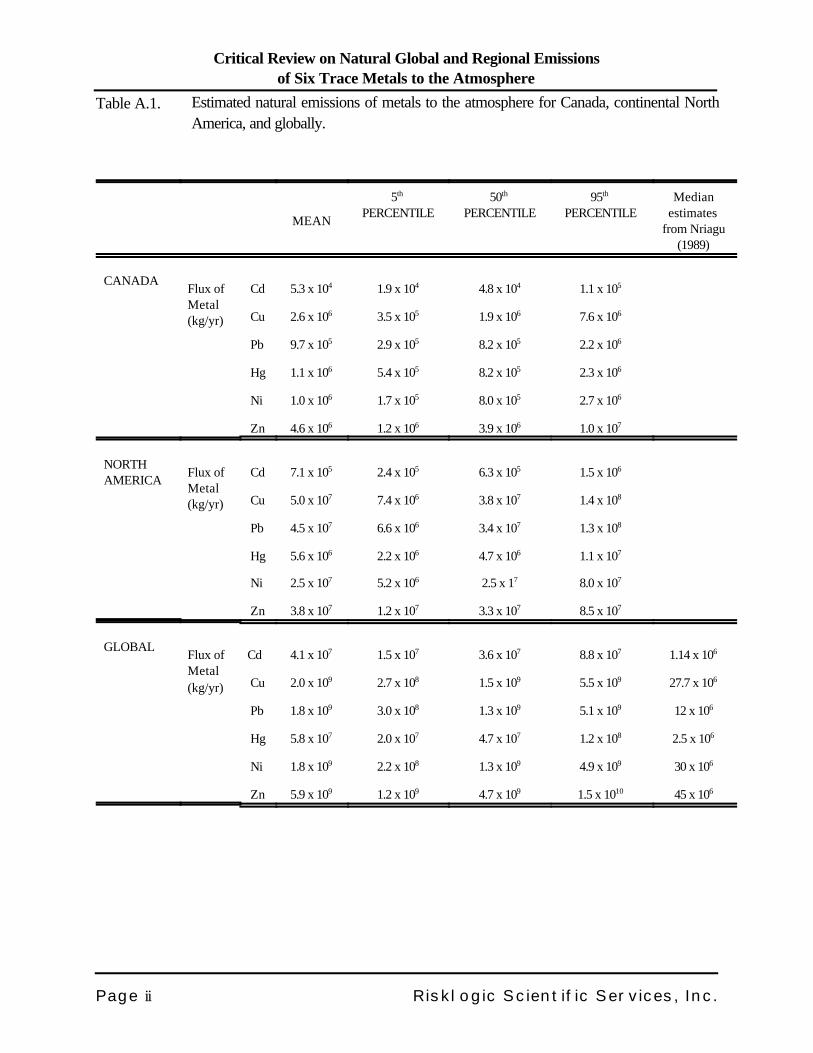
For Cd, Cu, Pb, Ni and Zn, the entrainment of soil dust particles into the air is a predominant source ofnatural emissions to the atmosphere. For mercury, volcanic emissions of Hg vapour predominate. Totalnatural emissions estimates for each metal, for Canada, North America and the globe, are presented inTable A.1, along with the global estimates of Nriagu (1989) for comparison.

The most significant data gap identified was the lack of information to quantify biogenic emissions of metalsother than Hg. Data are required on the concentrations of non-volatile metals associated with volatileorganic substances emitted by terrestrial and marine vegetation to enable the quantification of metalemissions from this natural source. Also, data are required to establish reliable enrichment factors to seasalt spray from sea water for both nickel and zinc.


Page ii Risklogic Scientific Services, Inc.

Table A.1. Estimated natural emissions of metals to the atmosphere for Canada, continental NorthAmerica, and globally.

MEAN

5th PERCENTILE

50th PERCENTILE

95th PERCENTILE

Medianestimates

from Nriagu(1989)

CANADAFlux ofMetal(kg/yr)

Cd 5.3 x 104 1.9 x 104 4.8 x 104 1.1 x 105

Cu 2.6 x 106 3.5 x 105 1.9 x 106 7.6 x 106

Pb 9.7 x 105 2.9 x 105 8.2 x 105 2.2 x 106

Hg 1.1 x 106 5.4 x 105 8.2 x 105 2.3 x 106

Ni 1.0 x 106 1.7 x 105 8.0 x 105 2.7 x 106

Zn 4.6 x 106 1.2 x 106 3.9 x 106 1.0 x 107

NORTHAMERICA

Flux ofMetal(kg/yr)

Cd 7.1 x 105 2.4 x 105 6.3 x 105 1.5 x 106

Cu 5.0 x 107 7.4 x 106 3.8 x 107 1.4 x 108

Pb 4.5 x 107 6.6 x 106 3.4 x 107 1.3 x 108

Hg 5.6 x 106 2.2 x 106 4.7 x 106 1.1 x 107

Ni 2.5 x 107 5.2 x 106 2.5 x 17 8.0 x 107

Zn 3.8 x 107 1.2 x 107 3.3 x 107 8.5 x 107

GLOBALFlux ofMetal(kg/yr)

Cd 4.1 x 107 1.5 x 107 3.6 x 107 8.8 x 107 1.14 x 106

Cu 2.0 x 109 2.7 x 108 1.5 x 109 5.5 x 109 27.7 x 106

Pb 1.8 x 109 3.0 x 108 1.3 x 109 5.1 x 109 12 x 106

Hg 5.8 x 107 2.0 x 107 4.7 x 107 1.2 x 108 2.5 x 106

Ni 1.8 x 109 2.2 x 108 1.3 x 109 4.9 x 109 30 x 106

Zn 5.9 x 109 1.2 x 109 4.7 x 109 1.5 x 1010 45 x 106


Page iii Risklogic Scientific Services, Inc.

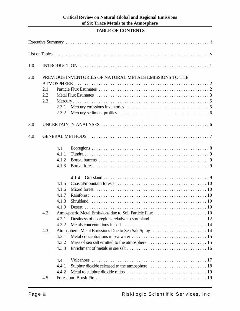
TABLE OF CONTENTS

Executive Summary . . . . . . . . . . . . . . . . . . . . . . . . . . . . . . . . . . . . . . . . . . . . . . . . . . . . . . . . . . . . . i

List of Tables . . . . . . . . . . . . . . . . . . . . . . . . . . . . . . . . . . . . . . . . . . . . . . . . . . . . . . . . . . . . . . . . . . v

1.0 INTRODUCTION . . . . . . . . . . . . . . . . . . . . . . . . . . . . . . . . . . . . . . . . . . . . . . . . . . . . . . . 1

2.0 PREVIOUS INVENTORIES OF NATURAL METALS EMISSIONS TO THEATMOSPHERE . . . . . . . . . . . . . . . . . . . . . . . . . . . . . . . . . . . . . . . . . . . . . . . . . . . . . . . . . 22.1 Particle Flux Estimates . . . . . . . . . . . . . . . . . . . . . . . . . . . . . . . . . . . . . . . . . . . . . . . 22.2 Metal Flux Estimates . . . . . . . . . . . . . . . . . . . . . . . . . . . . . . . . . . . . . . . . . . . . . . . . 32.3 Mercury . . . . . . . . . . . . . . . . . . . . . . . . . . . . . . . . . . . . . . . . . . . . . . . . . . . . . . . . . . 5

2.3.1 Mercury emissions inventories . . . . . . . . . . . . . . . . . . . . . . . . . . . . . . . . . . . 52.3.2 Mercury sediment profiles . . . . . . . . . . . . . . . . . . . . . . . . . . . . . . . . . . . . . . 6

3.0 UNCERTAINTY ANALYSES . . . . . . . . . . . . . . . . . . . . . . . . . . . . . . . . . . . . . . . . . . . . . . 6

4.0 GENERAL METHODS . . . . . . . . . . . . . . . . . . . . . . . . . . . . . . . . . . . . . . . . . . . . . . . . . . . 7

4.1 Ecoregions . . . . . . . . . . . . . . . . . . . . . . . . . . . . . . . . . . . . . . . . . . . . . . . . . . 84.1.1 Tundra . . . . . . . . . . . . . . . . . . . . . . . . . . . . . . . . . . . . . . . . . . . . . . . . . . . . . 94.1.2 Boreal barrens . . . . . . . . . . . . . . . . . . . . . . . . . . . . . . . . . . . . . . . . . . . . . . . 94.1.3 Boreal forest . . . . . . . . . . . . . . . . . . . . . . . . . . . . . . . . . . . . . . . . . . . . . . . . 9

4.1.4 Grassland . . . . . . . . . . . . . . . . . . . . . . . . . . . . . . . . . . . . . . . . . . . . . 94.1.5 Coastal/mountain forests . . . . . . . . . . . . . . . . . . . . . . . . . . . . . . . . . . . . . . . 104.1.6 Mixed forest . . . . . . . . . . . . . . . . . . . . . . . . . . . . . . . . . . . . . . . . . . . . . . . 104.1.7 Rainforest . . . . . . . . . . . . . . . . . . . . . . . . . . . . . . . . . . . . . . . . . . . . . . . . . 104.1.8 Shrubland . . . . . . . . . . . . . . . . . . . . . . . . . . . . . . . . . . . . . . . . . . . . . . . . . 104.1.9 Desert . . . . . . . . . . . . . . . . . . . . . . . . . . . . . . . . . . . . . . . . . . . . . . . . . . . . 10

4.2 Atmospheric Metal Emissions due to Soil Particle Flux . . . . . . . . . . . . . . . . . . . . . . 104.2.1 Dustiness of ecoregions relative to shrubland . . . . . . . . . . . . . . . . . . . . . . . . 124.2.2 Metals concentrations in soil . . . . . . . . . . . . . . . . . . . . . . . . . . . . . . . . . . . . 14

4.3 Atmospheric Metal Emissions Due to Sea Salt Spray . . . . . . . . . . . . . . . . . . . . . . . 144.3.1 Metal concentrations in sea water . . . . . . . . . . . . . . . . . . . . . . . . . . . . . . . . 154.3.2 Mass of sea salt emitted to the atmosphere . . . . . . . . . . . . . . . . . . . . . . . . . 154.3.3 Enrichment of metals in sea salt . . . . . . . . . . . . . . . . . . . . . . . . . . . . . . . . . . 16

4.4 Volcanoes . . . . . . . . . . . . . . . . . . . . . . . . . . . . . . . . . . . . . . . . . . . . . . . . . 174.4.1 Sulphur dioxide released to the atmosphere . . . . . . . . . . . . . . . . . . . . . . . . . 184.4.2 Metal to sulphur dioxide ratios . . . . . . . . . . . . . . . . . . . . . . . . . . . . . . . . . . 19

4.5 Forest and Brush Fires . . . . . . . . . . . . . . . . . . . . . . . . . . . . . . . . . . . . . . . . . . . . . . 19


Page iv Risklogic Scientific Services, Inc.

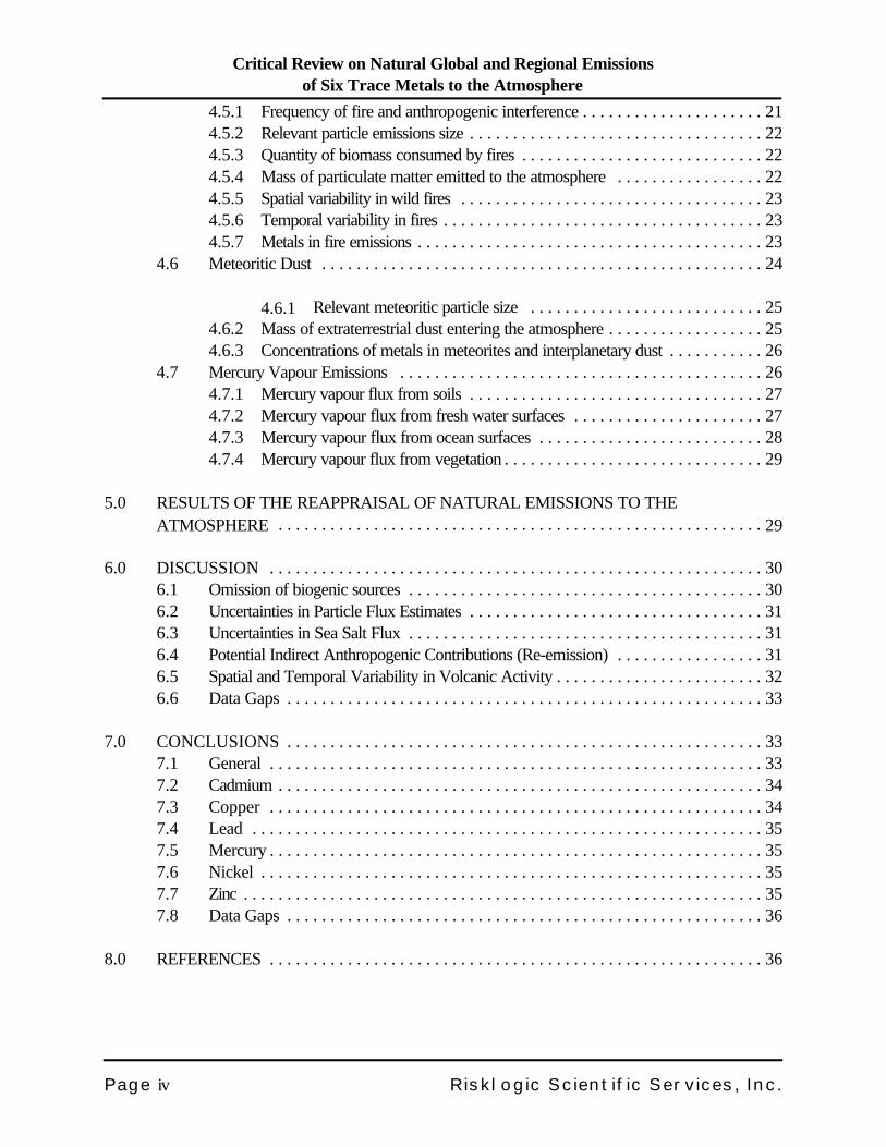
4.5.1 Frequency of fire and anthropogenic interference . . . . . . . . . . . . . . . . . . . . . 214.5.2 Relevant particle emissions size . . . . . . . . . . . . . . . . . . . . . . . . . . . . . . . . . . 224.5.3 Quantity of biomass consumed by fires . . . . . . . . . . . . . . . . . . . . . . . . . . . . 224.5.4 Mass of particulate matter emitted to the atmosphere . . . . . . . . . . . . . . . . . 224.5.5 Spatial variability in wild fires . . . . . . . . . . . . . . . . . . . . . . . . . . . . . . . . . . . 234.5.6 Temporal variability in fires . . . . . . . . . . . . . . . . . . . . . . . . . . . . . . . . . . . . . 234.5.7 Metals in fire emissions . . . . . . . . . . . . . . . . . . . . . . . . . . . . . . . . . . . . . . . . 23

4.6 Meteoritic Dust . . . . . . . . . . . . . . . . . . . . . . . . . . . . . . . . . . . . . . . . . . . . . . . . . . . 24

4.6.1 Relevant meteoritic particle size . . . . . . . . . . . . . . . . . . . . . . . . . . . 254.6.2 Mass of extraterrestrial dust entering the atmosphere . . . . . . . . . . . . . . . . . . 254.6.3 Concentrations of metals in meteorites and interplanetary dust . . . . . . . . . . . 26

4.7 Mercury Vapour Emissions . . . . . . . . . . . . . . . . . . . . . . . . . . . . . . . . . . . . . . . . . . 264.7.1 Mercury vapour flux from soils . . . . . . . . . . . . . . . . . . . . . . . . . . . . . . . . . . 274.7.2 Mercury vapour flux from fresh water surfaces . . . . . . . . . . . . . . . . . . . . . . 274.7.3 Mercury vapour flux from ocean surfaces . . . . . . . . . . . . . . . . . . . . . . . . . . 284.7.4 Mercury vapour flux from vegetation . . . . . . . . . . . . . . . . . . . . . . . . . . . . . . 29

5.0 RESULTS OF THE REAPPRAISAL OF NATURAL EMISSIONS TO THEATMOSPHERE . . . . . . . . . . . . . . . . . . . . . . . . . . . . . . . . . . . . . . . . . . . . . . . . . . . . . . . . 29

6.0 DISCUSSION . . . . . . . . . . . . . . . . . . . . . . . . . . . . . . . . . . . . . . . . . . . . . . . . . . . . . . . . . 306.1 Omission of biogenic sources . . . . . . . . . . . . . . . . . . . . . . . . . . . . . . . . . . . . . . . . . 306.2 Uncertainties in Particle Flux Estimates . . . . . . . . . . . . . . . . . . . . . . . . . . . . . . . . . . 316.3 Uncertainties in Sea Salt Flux . . . . . . . . . . . . . . . . . . . . . . . . . . . . . . . . . . . . . . . . . 316.4 Potential Indirect Anthropogenic Contributions (Re-emission) . . . . . . . . . . . . . . . . . 316.5 Spatial and Temporal Variability in Volcanic Activity . . . . . . . . . . . . . . . . . . . . . . . . 326.6 Data Gaps . . . . . . . . . . . . . . . . . . . . . . . . . . . . . . . . . . . . . . . . . . . . . . . . . . . . . . . 33

7.0 CONCLUSIONS . . . . . . . . . . . . . . . . . . . . . . . . . . . . . . . . . . . . . . . . . . . . . . . . . . . . . . . 337.1 General . . . . . . . . . . . . . . . . . . . . . . . . . . . . . . . . . . . . . . . . . . . . . . . . . . . . . . . . . 337.2 Cadmium . . . . . . . . . . . . . . . . . . . . . . . . . . . . . . . . . . . . . . . . . . . . . . . . . . . . . . . . 347.3 Copper . . . . . . . . . . . . . . . . . . . . . . . . . . . . . . . . . . . . . . . . . . . . . . . . . . . . . . . . . 347.4 Lead . . . . . . . . . . . . . . . . . . . . . . . . . . . . . . . . . . . . . . . . . . . . . . . . . . . . . . . . . . . 357.5 Mercury . . . . . . . . . . . . . . . . . . . . . . . . . . . . . . . . . . . . . . . . . . . . . . . . . . . . . . . . . 357.6 Nickel . . . . . . . . . . . . . . . . . . . . . . . . . . . . . . . . . . . . . . . . . . . . . . . . . . . . . . . . . . 357.7 Zinc . . . . . . . . . . . . . . . . . . . . . . . . . . . . . . . . . . . . . . . . . . . . . . . . . . . . . . . . . . . . 357.8 Data Gaps . . . . . . . . . . . . . . . . . . . . . . . . . . . . . . . . . . . . . . . . . . . . . . . . . . . . . . . 36

8.0 REFERENCES . . . . . . . . . . . . . . . . . . . . . . . . . . . . . . . . . . . . . . . . . . . . . . . . . . . . . . . . . 36


Page v Risklogic Scientific Services, Inc.

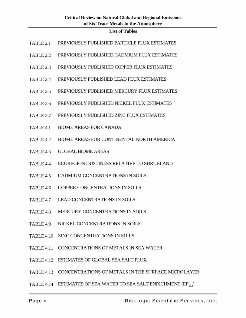
List of Tables

TABLE 2.1 PREVIOUSLY PUBLISHED PARTICLE FLUX ESTIMATES

TABLE 2.2 PREVIOUSLY PUBLISHED CADMIUM FLUX ESTIMATES

TABLE 2.3 PREVIOUSLY PUBLISHED COPPER FLUX ESTIMATES

TABLE 2.4 PREVIOUSLY PUBLISHED LEAD FLUX ESTIMATES

TABLE 2.5 PREVIOUSLY PUBLISHED MERCURY FLUX ESTIMATES

TABLE 2.6 PREVIOUSLY PUBLISHED NICKEL FLUX ESTIMATES

TABLE 2.7 PREVIOUSLY PUBLISHED ZINC FLUX ESTIMATES

TABLE 4.1 BIOME AREAS FOR CANADA

TABLE 4.2 BIOME AREAS FOR CONTINENTAL NORTH AMERICA

TABLE 4.3 GLOBAL BIOME AREAS

TABLE 4.4 ECOREGION DUSTINESS RELATIVE TO SHRUBLAND

TABLE 4.5 CADMIUM CONCENTRATIONS IN SOILS

TABLE 4.6 COPPER CONCENTRATIONS IN SOILS

TABLE 4.7 LEAD CONCENTRATIONS IN SOILS

TABLE 4.8 MERCURY CONCENTRATIONS IN SOILS

TABLE 4.9 NICKEL CONCENTRATIONS IN SOILS

TABLE 4.10 ZINC CONCENTRATIONS IN SOILS

TABLE 4.11 CONCENTRATIONS OF METALS IN SEA WATER

TABLE 4.12 ESTIMATES OF GLOBAL SEA SALT FLUX

TABLE 4.13 CONCENTRATIONS OF METALS IN THE SURFACE MICROLAYER

TABLE 4.14 ESTIMATES OF SEA WATER TO SEA SALT ENRICHMENT (EFsea)


Page vi Risklogic Scientific Services, Inc.

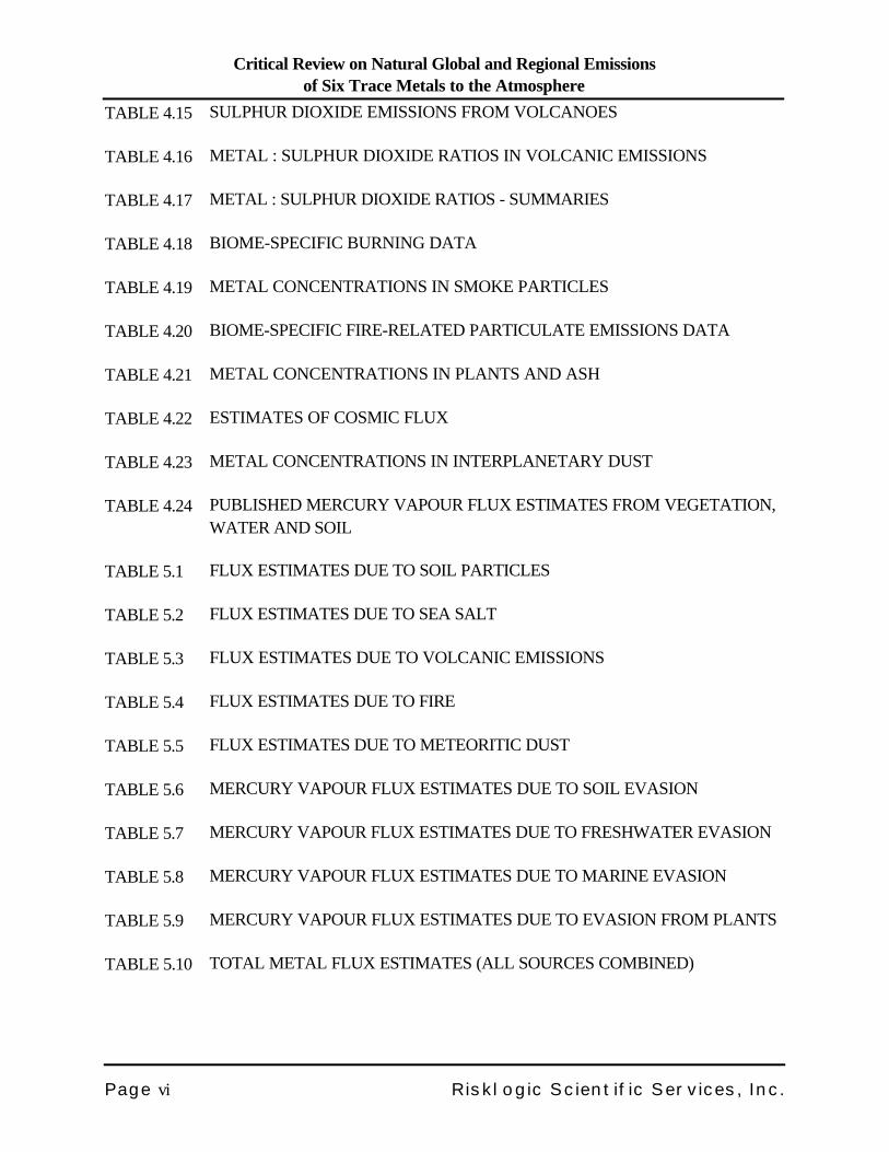
TABLE 4.15 SULPHUR DIOXIDE EMISSIONS FROM VOLCANOES

TABLE 4.16 METAL : SULPHUR DIOXIDE RATIOS IN VOLCANIC EMISSIONS

TABLE 4.17 METAL : SULPHUR DIOXIDE RATIOS - SUMMARIES

TABLE 4.18 BIOME-SPECIFIC BURNING DATA

TABLE 4.19 METAL CONCENTRATIONS IN SMOKE PARTICLES

TABLE 4.20 BIOME-SPECIFIC FIRE-RELATED PARTICULATE EMISSIONS DATA

TABLE 4.21 METAL CONCENTRATIONS IN PLANTS AND ASH

TABLE 4.22 ESTIMATES OF COSMIC FLUX

TABLE 4.23 METAL CONCENTRATIONS IN INTERPLANETARY DUST

TABLE 4.24 PUBLISHED MERCURY VAPOUR FLUX ESTIMATES FROM VEGETATION,WATER AND SOIL

TABLE 5.1 FLUX ESTIMATES DUE TO SOIL PARTICLES

TABLE 5.2 FLUX ESTIMATES DUE TO SEA SALT

TABLE 5.3 FLUX ESTIMATES DUE TO VOLCANIC EMISSIONS

TABLE 5.4 FLUX ESTIMATES DUE TO FIRE

TABLE 5.5 FLUX ESTIMATES DUE TO METEORITIC DUST

TABLE 5.6 MERCURY VAPOUR FLUX ESTIMATES DUE TO SOIL EVASION

TABLE 5.7 MERCURY VAPOUR FLUX ESTIMATES DUE TO FRESHWATER EVASION

TABLE 5.8 MERCURY VAPOUR FLUX ESTIMATES DUE TO MARINE EVASION

TABLE 5.9 MERCURY VAPOUR FLUX ESTIMATES DUE TO EVASION FROM PLANTS

TABLE 5.10 TOTAL METAL FLUX ESTIMATES (ALL SOURCES COMBINED)


Page 1 Risklogic Scientific Services, Inc.

1.0 INTRODUCTION

There is on-going regulatory concern for metals in the environment, and numerous regulations have beenimplemented globally, or are being developed, to control or curtail industrial emissions to the atmosphere.Of particular concern are metals and metalloids (Sang and Lourie, 1997; Lin and Pehkonen, 1998; amongothers). However, the relative impact or contribution made by natural sources, versus those ofanthropogenic origin, is typically ignored in environmental regulation.

Metals are released into the environment from natural sources through a variety of processes includingvolcanic eruption, forest and brush fires, and wind-blown suspension of dust and sea salt spray (Nriagu,1989; Lin and Pehkonen, 1998; among others). Metals generally exist within the atmosphere as acomponent of particulate matter (de Mora et al., 1993). In the case of Hg, however, a significantproportion is also in the vapour phase, due to its volatility at typical ambient temperatures (de Mora et al.,1993; Schroeder et al., 1995; among others).

The primary citation concerning the contribution made by natural sources to environmental metalcontamination remains Nriagu (1989), although other authors have also attempted to quantify thisphenomenon (discussed and reviewed below). Nriagu (1989) presented an analysis of available datasuggesting that natural contributions of metals and metalloids make up generally less than 50% of the totalemissions to the atmosphere.

There is considerable uncertainty in previously-published estimates of atmospheric metals emissions;uncertainties that generally go unquantified, and often unmentioned. These uncertainties relate to theapplication of different quantification methods, to spatial and temporal variation in the data required topredict total atmospheric emissions, and to uncertainties introduced by less than complete knowledge ofemission sources, their characteristics, spatial extent and temporal variability.

Regulatory agencies are now preparing to introduce or enact legislative initiatives to reduce industrial metalemissions, with no clear understanding of the relative contributions of anthropogenic and natural sources,and the uncertainties therein. Such legislation has been conceived on the basis of these earlier uncertainestimates of natural source contributions. For example, Canada is developing pollution abatement initiativesfor Hg (soil, air and water quality guidelines, phase-out of products containing Hg, emissions reductiontargets, etc.) on the assumption that natural and anthropogenic sources contribute approximately equally(50:50) to the environmental Hg problem (L.Trip, Environment Canada, Hull, Quebec, personalcommunication). Some data indicate that planned reductions in Hg industrial emissions, withoutconsideration for natural sources, will result in no significant decline in levels of biotic contamination(Richardson and Currie, 2000). It is apparent, therefore, that a need exists to update the estimate of naturalsource contributions with the spate of recent research on the emission of elemental Hg from surface waters,soils, faults and geologic deposits.

In order to evaluate, more rigorously, the sustainable use of metals, it is essential that the contributions ofnatural releases to the atmosphere be updated to reflect the latest data, and that a statistically rigoroustreatment of these data be undertaken to quantify confidence limits and uncertainties in these estimates.



The purpose of this paper was twofold. First, recently-available information was incorporated to estimatenatural emissions of six metals to the atmosphere. Those metals were cadmium (Cd), copper (Cu), lead(Pb), mercury (Hg), nickel (Ni) and zinc (Zn). These emissions have been quantified locally (Canada),regionally (continental North America) and globally. Secondly, variability and uncertainty in the datarequired to quantitatively estimate emissions were subjected to a statistically-rigorous probabilistic analysisto derive confidence limits on those emission estimates.

2.0 PREVIOUS INVENTORIES OF NATURAL METALS EMISSIONS TO THEATMOSPHERE

2.1 Particle Flux Estimates

The emissions of metals other than Hg are mainly associated with particulate matter. Therefore, estimatesof metal fluxes are closely linked to estimates of primary particle fluxes. Previous emissions inventories forparticles are summarized in Table 2.1.

An early inventory of particle fluxes was developed by Hidy and Brock (1970). These estimates werebased on studies by other authors, and the particle flux due to forest fires was developed by extrapolatingfrom United States data. Peterson and Junge (1971) independently developed an inventory of totalparticulate emissions. They also estimated the proportion of the particles that would be less than 5 Fm indiameter. The Study of Man’s Impact on Climate (Matthews et al., 1971) presented global particulateemission inventories for particles <20 Fm diameter and particles <6Fm diameter. All of these inventorieswere based on the limited published data available at the time, and included broad assumptions andextrapolations from regional data (where necessary).

Another inventory of particulate emissions was developed by Lantzy and Mackenzie (1979). This inventorywas based on global flux estimates for individual pathways from several other authors. Prospero et al.(1983) compiled emissions inventories from several authors, mainly from the early 1970s. Pacyna (1986)presented ranges of global particulate fluxes based on other authors, including Andren and Nriagu (1979),Peterson and Junge (1971) and Study of Man’s Impact on Climate (Matthews et al., 1971). Mosher andDuce (1987) developed an independent particulate emissions inventory for volcanoes, sea salt and firesbased on available literature; their estimate for windblown dust was adapted from Prospero et al. (1983).

Regional particulate emission inventories have also been developed. Evans and Cooper (1980) estimatedparticulate fluxes from windblown dust and fires in the United States, including a breakdown by state.Environment Canada (1981a) published particle flux estimates for Canada, including breakdowns byprovince, biome and source (i.e., soil dust, sea salts, forest and brush fires, volcanoes, plants and micro-community systems).



The Environment Canada report relied heavily on previous work by Robinson and Robbins (1971), Davis(1974) and Jaenicke (1980), who determined that natural sources contributed 85% to 89% of theparticulate mass entrained into the atmosphere.

Windblown soil is one of the largest sources of natural metal emissions to the atmosphere (Pacyna, 1986).Through the process of weathering and erosion, metals that naturally occur in the Earth’s crust will also befound in soil. Hagen and Woodruff (1975) suggest that wind erosion is an important source of totalparticulate mass and high particulate concentrations in the atmosphere. Their estimates place this sourceof particulate emissions to the atmosphere on par with emissions from anthropogenic sources.

Several authors have estimated the amount of soil that is entrained into the atmosphere via the wind, withthe general range of 200-500 x 109 kg/yr globally (Nriagu, 1978; Schmidt and Andren, 1980). Nriagu(1989), to estimate metal fluxes to the atmosphere, used a soil flux range from a review paper preparedby Prospero et al. (1983). The maximum value of 500 x 109 kg/yr (commonly cited) is also cited inPeterson and Junge (1971) and is based on a value from an unpublished paper. The estimate wasextrapolated from a calculation made for the United States including agricultural and natural dust sources.Another source cited in Peterson and Junge (1971) derives the same value of 500 x 109 kg/yr based ondeep ocean sedimentation rates.

Duce (1995) conducted a review of more recent estimates of global soil flux, ranging from 1000-3000 x109 kg/yr. Duce (1995) suggests that these higher estimates are more accurate than previously publishedestimates, due to more frequent monitoring and more remote ocean stations monitoring long distance dustflux. Alfaro et al. (1998) cite a value for dust flux from the Sahara alone at 600 x 109 kg/yr. Although theSahara is a large contributor of wind blown dust, there are several other arid areas in the world thatproduce dust, suggesting that global emissions may be much higher.

2.2 Metal Flux Estimates

Previous metal emission inventories from natural sources are summarized in Tables 2.2 through 2.7. Theseinventories are generally based on particulate fluxes and estimated metal concentrations in the sourceparticulate material. In some cases, metal concentrations measured directly in airborne particles wereemployed.

These inventories of natural metal fluxes have not been consistent in the sources considered or in themethods employed to quantify those emissions. However, they generally show windblown dust, volcanicemissions, sea salt spray, fires and biogenic emissions as the main sources of atmospheric aerosols. Witha few exceptions, estimated metal fluxes from windblown dust and volcanoes have been relativelyconsistent between different inventories; estimated metal fluxes from other pathways have often varied byorders of magnitude. Metal fluxes from meteoritic dust were rarely considered in previous inventories.

In the late 1970's and early 1980's (Nriagu, 1978; Nriagu, 1980a,b,c), inventories generally used dataobtained by Curtin et al. (1974) for metals in residual ash and ashed plant exudates to calculate fluxes fromforest fires and biogenic emissions. However, these data were collected from conifers in areas with



anomalously high metal concentrations in soils or plants, and are not likely representative of typical metalsconcentrations in those media. Emissions due to sea salt spray were based on concentrations of metals insea water and published enrichment factors of the metal from sea water to sea salt. However, theenrichment factors appear to have been used incorrectly in many cases (see Section 4.3). Volcanicemissions were based on crustal metal concentrations and published enrichment factors for metalenrichment in fine particulate matter. Zoller (1984) and Pacyna (1986) have summarized emissionsinventories from other authors.

Lantzy and Mackenzie (1979) published an inventory of metal fluxes in which the volcanic emissions werebased on concentrations in andesites (for volcanic particles) and gases from volcanoes, hot springs andfumaroles (for volcanic gases). The emissions due to fires were based on metal concentrations measuredin land plants.

Nriagu (1978) adapted the Hidy and Brock (1970) and Peterson and Junge (1971) particle flux inventoriesfor his metal flux estimates, though he used a lower meteorite dust flux estimated by Hindley (1976). Hegenerally used the same particle fluxes in later publications during the late 1970's and early 1980's, thoughhis inventories for copper (Nriagu, 1980b) and zinc (Nriagu and Davidson, 1980) used a lower flux forvolcanogenic particles, and his inventory for Hg used a higher value for the flux from vegetation (Andrenand Nriagu, 1979).

Jaworowski et al. (1981) developed natural metal emission inventories using two different approaches. Oneof these approaches was generally similar to the other inventories discussed above, though the emissionsfrom forest fires, volcanoes and meteoritic dust were based on extrapolations using soil metalconcentrations rather than metal concentrations specific to the sources of interest. The second approachwas based on a back extrapolation from concentrations of metals and radionuclides in glacier ice; thissecond method resulted in metal flux estimates orders of magnitude higher than estimates based onparticulate flux.

Nriagu (1989) published a revised metal emissions inventory based on particulate fluxes. These estimates,still frequently cited, were based on more recent data than his earlier publications. The basis for hisinventory was as follows:

• windblown dust emissions were based on estimates of wind-borne soil particles combined withconcentrations of metals in soil;

• sea salt spray emissions were based on estimated global sea salt flux, concentrations of metals insea water, and enrichment factors for the metals from sea water to sea salt; the enrichment factorsused were generally lower than those reported in the source literature;

• volcanic emissions were based on estimated sulphur emissions from volcanoes and published metal: sulphur ratios;

• wild forest fire emissions were based on biomass consumed by forest fires, metal concentrationsin plants and assumed burning yields for metals;

• continental biogenic metal emissions were based on particulate organic carbon concentrations,aerosol deposition, and metal concentrations in plants; and



• biogenic emissions of metals complexed with volatiles were based on estimated hydrocarbon fluxesfrom terrestrial and marine plants and metal concentrations in surface organic microlayers of aquaticecosystems.

Various data suggest that the natural metal fluxes to the atmosphere may be under-estimated by the Nriagu(1989) study:

• the atmospheric soil flux from the central United States alone (Hagen and Woodruff, 1975)appears to be of the same magnitude as the global flux reported by Nriagu (1989);

• the sea salt enrichment factors used by Nriagu were generally lower than those found in otherliterature (see Table 4.14); Nriagu (1989) did not specifically present the metal concentrations insea water employed in his calculations, so those calculations could not be duplicated or confirmed;

• there are now more recent data available on sulphur flux and metal to sulphur ratios (see Tables4.15 and 4.16) for revised predictions of emissions from volcanic emissions;

• for emissions due to fires, recent studies have measured actual concentrations of metals in smokeparticulate (see Table 4.19) (rather than relying on concentrations in non-combusted wood andvegetation); as well, more refined estimates of the quantity of biomass burned (see Table 4.18) andparticulate emissions (see Table 4.20) have been published; and

• measurements of Hg vapour emissions from vegetation, and more refined estimates of biogenicemissions of Hg (see Table 4.24), have been recently published.

2.3 Mercury

Additional comment on Hg is warranted given its release from natural sources as both particulate matterand vapour.

To date, two primary approaches have been employed to estimate the relative contributions ofanthropogenic and natural sources of Hg to the atmosphere: source inventories and dated lake sedimentcores.

2.3.1 Mercury emissions inventories

On a global basis, previous source inventories have been used to estimate that anthropogenic sourcescontribute between 50% and 75% of total annual atmospheric Hg loadings (reviewed by Fitzgerald, 1995;see also Fitzgerald, 1986; Lindqvist et al., 1991; Nriagu, 1989). By difference, natural sources would thencontribute between 25% and 50% of total global atmospheric loadings. On a more regional scale, however,available source inventories suggest that natural sources (involving gaseous and particulate emissions fromland and water surfaces) can contribute anywhere from only about 13% of total atmospheric loadings(estimated within the province of Ontario, Canada; Innanen, 1998) up to 80% of atmospheric Hgconcentrations (for Sweden; Brosset, 1981). Unfortunately, the reliability (quality and quantity) of dataupon which natural source Hg emissions estimates are based is far less than that for industrial emissions,the latter having been the subject of quantitative industrial emissions inventories in numerous countries formore than a decade.



Various authors have estimated the annual global Hg flux, or reviewed estimates by other authors, fromvarious natural sources. These authors include Ebinghaus et al. (1999), Rasmussen (1994a), Lindqvist etal. (1991), Nriagu (1989), Pacyna (1986, 1987), Zoller (1984), Jaworowski et al. (1981), and Lantzy andMackenzie (1979). Regional inventories of natural Hg emissions have been presented by Innanen (1998;for Ontario, Canada) and Vasiliev et al. (1998; for Siberia). These estimates are summarized in Table 2.5.

Since the mid-1980's, quantification of global emissions of Hg to the atmosphere has suggestedapproximately equal contributions from natural and anthropogenic sources, with the analysis presented byNriagu (1989) remaining the primary citation on the contributions of natural emissions of Hg to the globalatmosphere. For example, the analysis of Nriagu (1989) is the primary basis upon which EnvironmentCanada has assumed that natural sources contribute between 40% and 50% of total annual Hg emissionsto the Canadian atmosphere (L. Trip, Environment Canada, personal communication). Unfortunately,previous analyses have not attempted to quantify the uncertainty in these estimates, beyond providingapproximate minima and maxima around predicted mean or modal values. The potential range betweenminimum and maximum natural source emissions can be quite large, however (see Table 2.5).

2.3.2 Mercury sediment profiles

Profiles of Hg concentration by depth in sediment cores from remote lakes (lakes not affected by directindustrial discharges or impoundment) have also been put forward as evidence of the significant increasein industrial emissions of Hg in the past century (Fitzgerald et al., 1998). Examination of published data fromOntario lakes (Evans, 1986; Johnson et al., 1986; Johnson, 1987; Rasmussen et al., 1998a) suggests thatHg deposition from the atmosphere to these lakes has increased anywhere from less than 2 times to asmuch as 10 times over the past 100 to 150 years. This suggests that the natural source component of thisatmospheric deposition could range from more than 50% to less than 10%.

Not only does this ratio of surficial (recent) sediment Hg concentration to deep (purported pre-industrialor natural) sediment Hg concentration vary several fold, but it varies several fold between lakes situatedin close proximity to one another. The atmospheric deposition of industrial Hg emissions to lakes is knownto decline with increasing distance from point sources (EPMAP, 1994). However, lakes in close proximityto one another are also more or less equally distant from significant industrial point sources. Therefore,distance from point sources does not explain all of the inter-lake variation in Hg sedimentation rates. Thisinter-lake variation in apparent anthropogenic Hg sedimentation indicates that Hg concentration in lakesediments is influenced by factors other than simply atmospheric inputs. One confounding factor may beearly diagenesis (Matty and Long, 1995), which is controlled by sediment organic matter content and otherchemical and geochemical characteristics that vary from lake to lake. Although the significance, and eventhe existence, of this phenomenon is debated (Fitzgerald et al., 1998; Rasmussen, 1998a), it is clearlyevident that the content of organic matter in sediments explains a great deal of the inter-lake variability insediment Hg concentrations among lakes in relatively close proximity (Rasmussen et al., 1998a). As aresult, it is apparent that Hg sediment profiles provide an inadequate basis for quantifying the relativecontributions of natural versus anthropogenic sources of the Hg that is ultimately deposited to lakesediments.



3.0 UNCERTAINTY ANALYSES

As indicated throughout the Methods section (below), variables necessary to calculate natural emissionsof metals to the atmosphere were defined in terms of a distribution, spanning values from the likely minimumthrough the likely maximum. In order to derive confidence limits for estimates of natural emissions to theatmosphere, a statistically rigorous approach to data analysis was required. In order to achieve this,probabilistic (stochastic) methods were employed.

Probabilistic uncertainty analyses were carried out in order to evaluate the influence of simultaneous,independent variations in several equation variables. Data such as concentrations of metals in soilparticulate matter, sea salt, etc. are not constant, but range over several orders of magnitude, dependingon geographic setting and numerous other factors. The ranges of possible values are best represented bydistributions or probability density functions.

The exact form of the probability distribution for many of the parameters is not known. Therefore,triangular distributions have been assigned to most of the variables, defined in terms of the upper and lowerlimits and the modal or most likely value. Triangular distributions are recommended when data areinsufficient to define the true data distribution, or when the underlying distribution type is known (log-normal, say) but data are insufficient to accurately quantify all distributional characteristics and parameters(Finley et al., 1994).

Using a form of Monte Carlo simulation, multiple iterations of flux calculations were conducted whilerandomly sampling from the distributions of input variables. A population of equation solutions was therebygenerated, resulting in a probability distribution for the calculated fluxes from which the mean value and the5th, 50th (median) and 95th percentiles of the flux distributions were estimated. The 5th and 95th percentilestatistics represent robust estimates of the upper and lower 90% confidence limits for the estimated meanand median flux values. For each simulation, a Latin hypercube sampling method was used and 20 000iterations were performed using Microsoft Excel97® (Microsoft Corp., 1996) and Crystal Ball ®(Decisioneering Inc., 1996), software.

4.0 GENERAL METHODS

Consistent with the earlier work of Nriagu (1989), five natural sources of metals emissions to theatmosphere were considered herein for Cd, Cu, Pb, Ni and Zn:

• wind-borne soil particles;• sea salt spray;• volcanoes;• forest and brush fires;• meteoritic (extra-terrestrial) dust.



The atmospheric emissions of Cd, Cu, Pb, Ni and Zn due to biogenic processes could not be calculateddue to insufficient data on metal concentrations in volatile plant exudates. This is discussed further in section8 (Discussion).

In addition to particulate-borne emissions of Hg, direct evasion of vapour also occurs from surface waters,soil, geologic deposits and vegetation. Therefore, nine natural sources of Hg emission to the atmospherewere considered:

• Hg vapour (Hg0) flux from soils and bedrock;• Hg0 flux from surface marine waters;• Hg0 flux from surface fresh waters;• volcanic emissions (both gaseous and particulate Hg);• wind-induced entrainment of surficial soil and dust particles;• wind-induced entrainment of sea salt spray;• forest and brush fires;• meteoritic (extra-terrestrial) dust;• Hg0 flux directly from vegetation (biogenic emissions ).

Nriagu (1989) recognized the potential biogenic emission of Hg vapour from vegetation. However, no dataexisted at that time to directly quantify such emissions. Therefore, Nriagu (1989) necessarily extrapolatedfrom published data on hydrocarbon emissions from plants, combined with measured fluxes of methylatedHg compounds and available data on the ratio of Hg vapour concentration and hydrocarbon concentrationas reported for urban, rural and remote air samples. Recent advances in the measurement of vegetative Hgemissions has lead to speculation that natural emissions of Hg may be under-estimated by as much as 100%(Lindberg et al., 1998).

Also, the accurate quantification of Hg vapour flux from soils and bedrock is a recent (< 5 years)development and that recent research permits the direct quantification of Hg flux to the atmosphere as afunction of soil Hg concentration (see Rassmussen et al., 1998b, for example).

Nriagu (1989) did not specifically quantify Hg emissions emanating from bodies of fresh water. However,recent research permits the quantification of this flux, accounting for seasonal variability due to the influenceof ambient temperature.

Specific equations and data reviewed to quantify natural emissions are outlined in greater detail below. Thefirst step, however, was to divide the regions under consideration (Canada, continental North America,Globe) into specific biomes or ecoregions, each of which has unique vegetative characteristics, leading tounique atmospheric particle flux rates, unique fire frequency, etc.



4.1 Ecoregions

The total areas of Canada, continental North America and the globe that encompass nine prescribedecoregions are presented in Tables 4.1 through 4.3. General descriptions of the different ecoregions areprovided below.

For Canada, two sources of information were used to define ecoregions - Environment Canada (1981a)and Clayton et al. (1977). The ecoregion areas in both reports were quite similar. Therefore, they wereaveraged together to obtain mean values for surface area covered. In the case of the grassland ecoregion,that defined by Clayton et al. (1977) comprised 3 of Environment Canada’s ecoregions - Eastern CanadaGrassland, Agricultural Grassland (Prairies and BC) and Aspen Parkland. To simplify the proposedecoregion scheme, the grassland scheme of Clayton et al. (1977) was used.

For continental North America, data from Leenhouts (1998) provided detailed information on vegetationcover in the United States. That information was reviewed in conjunction with an ecoregion map preparedby the United States Geological Survey (Eastern Energy and Land Use Team, 1982) which usedecoregions as described by Bailey (1998). These two sources were used to define ecoregions in the UnitedStates. The nine ecoregions defined for Canada and the U.S. were simply added to derive total areas foreach ecoregion in continental North America.

Different researchers have used varying criteria in categorizing the global land surface into ecoregions(Guenther et al., 1995; Bailey, 1998; Hannah et al., 1995; and Pears, 1985). Categories defined by Bailey(1998) most closely resemble the ecoregion scheme used herein. In addition, Bailey (1998) provides adetailed map by which to gain a geographical understanding of the ecoregions. Therefore, Bailey’s (1998)data were used herein to estimate world ecoregion areas.

The estimated total surface area of each ecoregion changes temporally due to changing climatic factors,deforestation, etc. Also, the estimation of ecoregion surface area varies from one author to another dueto varying estimation methods and data employed. However, for the purpose of the analysis presentedherein, the area of each ecoregion was assumed to be constant (fixed) so as not to unduly influence theuncertainty analysis.

4.1.1 Tundra

The tundra region occupies the northernmost regions of the northern hemisphere and southernmost regionsof the southern hemisphere. It is characterized by a cold climate, general absence of trees, and anintermittent ground covering of lichens, mosses, and sedges (Clayton et al.,1977). For the purposes of thisstudy, it also includes areas classified as arctic deserts. It includes 14.1 x 106 km2 of ice covered areas suchas Greenland and the Antarctic, and the islands in northern Canada (Bailey, 1998).



4.1.2 Boreal barrens

The boreal barrens refers to the transition zone between the tundra and the boreal forest consisting of open,stunted coniferous forests, interspersed with tundra vegetation (Clayton et al., 1977). It includes areas suchas northwest Siberia, northwest Canada and Alaska (Bailey, 1998).

4.1.3 Boreal forest

The boreal forest ecoregion refers to the cool forest zone of mainly coniferous trees (dominated by sprucespecies) that occurs south of the tundra ecoregion (Clayton et al., 1977). It covers a wide band acrossCanada from coast to coast and into Alaska, and for this study includes the taiga regions across most ofRussia (Bailey, 1998).

4.1.4 Grassland

The grassland ecoregion is characterized by ground cover of a variety of grasses and sparse trees (Claytonet al., 1977). It covers agricultural areas, savannas, steppes and prairies. For the purposes of this report,groundcover dominated by grasses was the criteria for placing an area in this category. It was assumed thatsimilar ground cover would allow similar soil exposure to wind, and similar fire conditions. Also includedin this category were the humid savannas of central South America, south central Africa, India and theCarribean. These latter areas are dominated by grasses, but may be somewhat more humid than grasslandsin North America. Aspen Parkland areas have been included in the grassland ecoregion because they arelargely fescue prairie (Clayton et al., 1977) and they were not segregated by Bailey (1998).

4.1.5 Coastal/mountain forests

The coastal/mountain ecoregion is characterized by a dominance of coniferous forests (mainly pine, cedarand fir species) in montane and coastal regions (Clayton et al., 1977). It includes areas in western NorthAmerica including the Rocky Mountains, mountainous regions in the southern portions of South America,and portions of Europe, the United Kingdom, New Zealand and Australia (Bailey, 1998).

4.1.6 Mixed forest

In Canada, the mixed forest ecoregion is comprised of the mixed forests surrounding the Great Lakesregion and the Acadian forest in the Maritimes. These forests consist of a mixture of deciduous andconiferous trees (Clayton et al., 1977). In North America, this region includes the Great Lakes forests, themixed forests in the northeastern United States and the mixed and deciduous forests in the southeasternUnited States. Deciduous forests are included in this category based on the assumption that amount andtype of vegetation cover is quite similar.



4.1.7 Rainforest

Rainforests are areas that receive significant annual rainfall and have a closed canopy of diverse evergreentrees with a lower layer of vines, palms and epiphytes (Brown and Gibson, 1983). Regions in this categoryinclude the Amazon Rainforest, Zaire and several smaller countries in west/central Africa along the coast,and Indonesia (Bailey, 1998).

4.1.8 Shrubland

This area is a mix between grassland, forest and desert. It is characterized by dry areas with Mediterraneanclimate, and includes chaparral, shrubland and dry woodlands. These areas have a dense mass of shrubscovering the ground and often have hot, dry summers (Brown and Gibson, 1983). Regions in this categoryinclude areas of the southwestern United States, central Africa, parts of Australia, and central/southwestAsia (Bailey, 1998).

4.1.9 Desert

Deserts are in the most arid parts of the world and receive little and/or sporadic rainfall. Vegetation is quitesparse and consists of scattered shrubs (Brown and Gibson, 1983). Desert areas are found in north Africa,the Middle East, Australia, south central Asia/northern China and in the southwestern United States (Bailey,1998).

4.2 Atmospheric Metal Emissions due to Soil Particle Flux

The flux of each element to the atmosphere due to suspension of soil particles was calculated as:

MF (kg/year) = 3 [AERi x PFERi x CSi x 10-6 kg/mg]

where, MF = metal flux to atmosphere (kg/yr)AERi = the area of ecoregion i (km2)PFERi = particulate flux to atmosphere from ecoregion i (kg/km2/yr)CSi = concentration of metal in soil of ecoregion i (mg/kg)

Based on an extensive review of available literature, only the shrubland ecoregion had published dataquantifying the soil particulate flux to the atmosphere. Several studies have been conducted on particlemovement during dust storms in the Great Plains of the central United States (Hagen and Woodruff, 1973,1975; Gillette et al.,1978).

The flux data reported by Hagen and Woodruff (1975) for the south central United States (Texas,Oklahoma, New Mexico, Kansas and Colorado) were selected to represent the shrubland ecoregion forthe following reasons:



1. Flux data were available for the south central United States for 2 decades (the 1950s and the1960s) while only 1950s data were available for the north central United States.

2. The Environment Canada (1981a) report suggests that the 1950s were an exceptionally drydecade. Therefore, using the flux data recorded over 2 decades (including the 1950s)wouldencompass the range of climate variability.

3. The land surface encompassed by the south central United States most closely resembles theshrubland ecoregion.

It should be noted that the values reported by Hagen and Woodruff (1975) are based on soil flux duringdusty hours only. A previous study by Hagen and Woodruff (1973) calculated that the south central UnitedStates was dusty 45 hours per year. Therefore, the Hagen and Woodruff (1975) soil fluxes were adjusted(multiplied by 0.005; i.e., [45 hours]/[8760 hours per year]) to obtain an annual soil flux in units ofkg/km2/yr for the shrubland ecoregion.

For the uncertainty analysis and determination of confidence limits of estimated emissions, variability in theelement concentrations in soil and the atmospheric flux of the soil particles for the different ecoregions wereconsidered.

For the uncertainty analysis, a triangular distribution was assigned to the particle flux value for the shrublandecoregion with the 1960s minimum value as the overall minimum value (526 kg/km2/yr), the 1950smaximum value as the overall maximum value (431 225 kg/km2/yr) and the mean of the 1950s and 1960sdata as the most likely value (61015 kg/km2/yr).

A study by Gillette et al. (1978) confirms the range of soil fluxes selected for the shrubland ecoregion.Gillette et al. (1978) measured dust flux during dust storms in Texas, reporting 0.3 to 0.5 million metric tonsof soil entrained per dust storm (measured at an altitude of 2.7 km and over an area of 5.7 x 1011 m2) whichresults in 527 to 877 kg/km2 dust particles released per storm. Assuming 3 storms per year (as per Gilletteet al., 1978), the annual soil flux would be 1578 to 2631 kg/km2/yr which falls within the low end of therange of fluxes calculated using the Hagen and Woodruff (1975) data. It should be noted that the Gilletteet al. (1978) data were measured at an altitude of 2.7 km which implies that their flux excludes thoseparticles with shorter atmospheric residence times.

4.2.1 Dustiness of ecoregions relative to shrubland

To quantify the atmospheric soil flux for the other ecoregions, a flux ratio, relative to shrubland, wasdetermined based on published dust storm day frequency data (see Table 4.4). It was assumed that theflux of soil particulate matter to the atmosphere in any given ecoregion was directly proportional to thefrequency of dust storms in that area. Therefore:

FDS-shrubland/FDS-ecoregioni = PFshrubland/PFecoregioni



OR

PFecoregioni = PFshrubland x FDS-ecoregioni/FDS-shrubland

where, FDS-shrubland = frequency of dust storms on shrublandFDS-ecoregioni = frequency of dust storms on ecoregion iPFshrubland = particle flux from shrublandPFecoregioni = particle flux from ecoregion i

Minimum, maximum and most likely values for the ratio FDS-ecoregioni/FDS-shrubland were calculated for eachecoregion from available data and are presented in Table 4.4.

There is very little information available on soil flux or frequency of dust storms for forested areas.Estimates by Middleton (1984) were used to evaluate the forested parts of Australia and data from Orgilland Sehmel (1976) were used to evaluate the forested parts of the United States. Estimates of dusty dayfrequency for forested areas predicted herein are much higher than those predicted by Environment Canada(1981a). Although Environment Canada (1981a) also used data from Orgill and Sehmel (1976), it remainsunclear as to how Environment Canada (1981a) arrived at their reported relative dust frequency forforested areas.

One problem with using dusty day frequencies as a basis for soil flux is that these data give no estimate ofthe volume of dust raised, the length of the storm nor the altitude to which the dust is raised (Middleton etal., 1986). As well, the dust observed in an area does not necessarily originate in that area. Orgill andSehmel (1976) suggest that much of the dust observed in mountainous areas and mixed forest areas in theUnited States originated elsewhere. Therefore, the estimated dustiness values for the coastal/mountainregion, mixed forest, and rainforest were arbitrarily reduced by a factor of 2, as done by EnvironmentCanada (1981a) in their calculations. There was no other information in the reviewed literature to suggesta different correction factor.

Based on the dust storm day data, a higher soil flux was calculated for the mixed forest ecoregion than forthe mountain/coastal forest ecoregion. Support for this conclusion comes from the Wind Erosion ResearchUnit (1999) which mapped the areas in the United States with wind erosion problems. The Pacific coastaland mountain areas showed very little erosion, while a large section in the southeastern United States (partof the mixed forest ecoregion) was subject to wind erosion.

For the rainforest ecoregion, a value of 0.077 dusty days/yr, relative to shrubland, was calculated from themaps of Australia (Middleton, 1984). This value is high due to the influence of one data location that hada much higher dust storm day frequency than the others. The only other data available for rainforests is avalue of 0 from Middleton (1986b) from a map showing the southern tip of India. Choosing a mostprobable value of 0.039 (0.077/2) relative to shrubland would indicate that rainforests are dustier thanmountain/coastal forests and mixed forests, which is unlikely. It is more likely there is hardly any dust fluxemitted from rainforests. Therefore, a triangular distribution was selected herein for the rainforest ecoregionwith minimum and most likely relative values of 0 and a maximum value of 0.039.



Estimates for dusty days on tundra were not found in the literature. In the tundra region, limited groundcover and trees will allow wind erosion to occur. However, much of this erosion can be attributed toblowing snow (Fristrup, 1952). Ashwell (1986) reports that dust storms do occur in central Iceland. Itseems reasonable that, due to lack of vegetation, and reports of dust storms, that tundra would be dustierthan mountain/coastal areas. However, over half of the estimated tundra area is permanently ice coveredfrom which there should be no dust emissions. Therefore, the tundra region dustiness was arbitrarilyestimated to be ½ of the value for the mountain/coastal ecoregion.

Estimates from minerogenic dust storm frequencies for boreal barrens and boreal forest were not found inthe literature. Nickling (1978) shows that dust storms do occur in boreal barrens areas, specifically in ariver valley delta in the Yukon Territory. However, the National Climate Data Center in the United States(NCDC, 2000) indicates 0 recorded dust storms from January 1, 1993 to June 30, 2000 for Alaska (alsoboreal barrens). This suggests that dust storms are possible in boreal barrens and boreal forest, but thatthey are not frequent. Boreal forest and boreal barrens have a similar coniferous type forest to the mountainregions and, therefore, were assigned the same dusty day frequency as mountain regions (i.e., 0.01 relativeto shrubland). Boreal barrens and boreal forest likely have a longer snow cover (especially whencompared to the coastal portion of the mountain/coastal region) and thus will likely have a maximumdustiness less than the maximum for the mountain/coastal ecoregion. A uniform distribution was chosenfor boreal barrens and boreal forest with 0 as the minimum and 0.01 as the maximum.

Mountainous, coastal and forested areas do not often experience dust storms (Orgill and Sehmel, 1976).In forested areas, the vegetation cover acts as a protective barrier against winds to prevent aeolian erosionand suspension of soil materials (Orgill and Sehmel, 1976). Brazel and Nickling (1987) report thatvegetation cover alters the aerodynamics of the air movement over the land and it requires a higher windspeed to raise dust. A large portion of the coastal mountains and rocky mountains in the northeasternUnited States have very low dust frequencies, with much of that dust originating elsewhere (Orgill andSehmel, 1976). The non-erosive materials of mountainous and other similar areas also leads to a minimalamount of soil suspension (Hagen and Woodruff, 1975).

4.2.2 Metals concentrations in soil

Data used herein on concentrations of metals in soils are summarized in Tables 4.5 through 4.10. Metalconcentrations in soil entrained into the atmosphere are equivalent to those found in surface soil (Eltayebet al., 1993). Canadian average concentrations for each metal were calculated by averaging all tabulateddata for Canada. North American values were obtained by taking a weighted average of the Canadian andUnited States data based on land area. Estimates for global metal concentrations in soil were calculatedby taking a weighted average of available data from various continents. In cases where data for a continentwere missing, average concentration data from other continents were assumed to be representative. Thevalues calculated for the world were comparable with world estimates made by various other sources.Average concentrations derived as described above were used as most likely values in triangulardistributions employed for uncertainty analysis. Minimum, maximum and most likely metals concentrationsused herein are detailed in Tables 4.5 through 4.10.



Data for the South Pacific were omitted from calculations for Ni concentrations because of anomalouslyhigh values (see Table 4.9). Hg data for Africa were also omitted due to anomalously low values (see Table4.8).

4.3 Atmospheric Metal Emissions Due to Sea Salt Spray

The flux of each element to the atmosphere through suspension of sea salt spray was calculated as:

MF (kg/year) = AOcean x SFOcean x [CSW /CNa] x EFSea x SSNa

where, MF = metal flux to atmosphere (kg/yr)AOcean = surface area of ocean (km2)SFOcean = sea salt spray flux to atmosphere from the ocean area considered (kg/km2-yr)CSW = concentration of metal in sea water (ng/L)CNa = concentration of sodium in sea water (ng/L)EFSea = enrichment factor for the concentration of the metal in sea water versus sea salt, relative

to the enrichment of sodium in sea water versus sea salt SSNa = concentration of sodium in sea salt (kg/kg)

Note: EFSea is not simply the relative concentration of the metal in sea salt versus sea water(discussed below).

In order to estimate the emission of Cd, Cu, Pb, Hg, Ni and Zn to the atmosphere in sea salt, the followingassumptions were employed:

• For the Canadian and North American estimates, the ocean surface area was considered to bedefined by international territorial limits (200 nautical miles from the coast). These areas wereprorated for seasonal ice cover to obtain annual average ice-free surface areas.

• The sea salt flux per unit ice-free area for Canada, North America and globally was assumed tobe equivalent, on a kg/km2/yr basis, although variation due to average wind speed, storms, etc.were considered within the uncertainty analysis.

• The concentrations of metals in the sea near Canada and North America were based on datacollected adjacent to North America, whereas all reviewed data were used for global averageconcentrations.

• Data from areas clearly polluted by anthropogenic effects (i.e., located near major industrialsources) were excluded.

For the uncertainty analysis, variability in element concentrations in sea water, sea water to sea saltenrichment factors and ocean surface emission rates of sea salt spray (as affected by storms, variation in



annual average wind speeds, etc.) were considered. The estimates of sea salt flux (as sodium) to theatmosphere was summarized by a triangular distribution defined from the minimum, modal and maximumvalues published in the literature. The enrichment factor was represented by a triangular distribution, withthe minimum enrichment factor of 1 (assumes that the ratio of the concentrations of the metal and sodium(Na) was the same in sea water and sea salt); the ‘most probable’ enrichment factors were taken as themedian of all published values (on a metal-by-metal basis) (see discussion below); and the maximumenrichment factor was taken as the maximum reported value in the literature. Triangular distributions weredeveloped for metal concentration data, using published values for Canadian, North American and globalaverage metal concentrations in sea water.

4.3.1 Metal concentrations in sea water

Measurements of metal concentrations in sea water are summarized in Table 4.11. Data suspected of beingaffected by nearby anthropogenic sources were excluded. Median values were used to represent “mostprobable” concentrations instead of mean values, since the data were not normally distributed.

4.3.2 Mass of sea salt emitted to the atmosphere

Available estimates of global sea salt flux are summarized in Table 4.12. Based on these estimates atriangular distribution (minimum, mode and maximum values) was developed to represent the global seasalt flux from the oceans on a kg/km2 /yr basis. Sea salt is emitted to the atmosphere through burstingbubbles at the water surface, and the rate of sea salt production is highly dependent on wind speed(Monahan, 1986). The salt is emitted from a thin microlayer at the ocean surface, which contains elevatedconcentrations of many metals when compared with the near-surface water (Duce et al., 1976).

The sea salt fluxes for Canadian and North American marine territories (defined by the internationalterritory boundaries) were calculated by multiplying published global fluxes by the ratio of the ocean areain the territorial boundaries to the total ocean area. Adjustment was also made in Canadian calculationsto account for areas of ice cover, from which salt spray is not expected. This was done by multiplying theactual area defined by the territorial boundaries by ice cover factors adapted from Environment Canada(1981a): 0.25 for the Arctic Ocean, 0.58 for the Atlantic Ocean north and east of Newfoundland and 0.83for the Canadian portion of the Atlantic Ocean south and west of Newfoundland.

4.3.3 Enrichment of metals in sea salt

Previous estimates of the contribution of sea salt flux to global metals emissions were calculated by Nriagu(1980a,b,c). In those papers, the metal flux due to sea salt spray was determined as:

MF = CSW x EF x FSS

where, MF = metal flux to the atmosphere (kg/yr)CSW = concentration of metal in sea water (mg/kg)EF = enrichment factor for metal between sea water and sea salt (mg/kg salt/mg/L water)



FSS = flux of sea salt to the atmosphere (kg/yr)

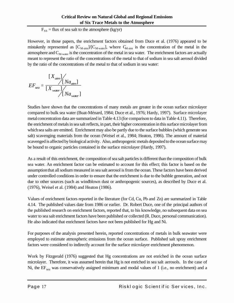
However, in those papers, the enrichment factors obtained from Duce et al. (1976) appeared to bemistakenly represented as [CM-atm]/[CM-water], where CM-atm is the concentration of the metal in theatmosphere and CM-water is the concentration of the metal in sea water. The enrichment factors are actuallymeant to represent the ratio of the concentrations of the metal to that of sodium in sea salt aerosol dividedby the ratio of the concentrations of the metal to that of sodium in sea water:

EF

XNa

XNa

sea

atm

atm

water

water

=

[ ][ ]

[ ][ ]

Studies have shown that the concentrations of many metals are greater in the ocean surface microlayercompared to bulk sea water (Buat-Ménard, 1984; Duce et al., 1976; Hardy, 1997). Surface microlayermetal concentration data are summarized in Table 4.13 (for comparison to data in Table 4.11). Therefore,the enrichment of metals in sea salt reflects, in part, their higher concentration in this surface microlayer fromwhich sea salts are emitted. Enrichment may also be partly due to the surface bubbles (which generate seasalt) scavenging materials from the ocean (Weisel et al., 1984; Heaton, 1986). The amount of materialscavenged is affected by biological activity. Also, anthropogenic metals deposited to the ocean surface maybe bound to organic particles contained in the surface microlayer (Hardy, 1997).

As a result of this enrichment, the composition of sea salt particles is different than the composition of bulksea water. An enrichment factor can be estimated to account for this effect; this factor is based on theassumption that all sodium measured in sea salt aerosol is from the ocean. These factors have been derivedunder controlled conditions in order to ensure that the enrichment is due to the bubble generation, and notdue to other sources (such as windblown dust or anthropogenic sources), as described by Duce et al.(1976), Weisel et al. (1984) and Heaton (1986).

Values of enrichment factors reported in the literature (for Cd, Cu, Pb and Zn) are summarized in Table4.14. The published values date from 1986 or earlier. Dr. Robert Duce, one of the principal authors ofthe published research on enrichment factors, reported that, to his knowledge, no subsequent data on seawater to sea salt enrichment factors have been published or collected (R. Duce, personal communication).He also indicated that enrichment factors have not been published for Hg and Ni.

For purposes of the analysis presented herein, reported concentrations of metals in bulk seawater wereemployed to estimate atmospheric emissions from the ocean surface. Published salt spray enrichmentfactors were considered to indirectly account for the surface microlayer enrichment phenomenon.

Work by Fitzgerald (1976) suggested that Hg concentrations are not enriched in the ocean surfacemicrolayer. Therefore, it was assumed herein that Hg is not enriched in sea salt aerosols. In the case ofNi, the EFsea was conservatively assigned minimum and modal values of 1 (i.e., no enrichment) and a



maximum value of 10, the value used by Nriagu (1989). The assumed maximum value of 10 is still muchlower than the measured EFsea values for other metals (see Table 4.14).

For purposes of calculating the metal fluxes, it was assumed herein that the mean concentration of sodiumin sea water was 10.6 g/L, and the concentration of sodium in sea salt was assumed to be 35% by weight(based on Duce et al., 1976, and Weisel et al., 1984).

Sea salt flux is highly dependent on wind speed, among other factors (Monahan, 1986). The estimates ofsea salt flux used herein were, of necessity, global averages. In addition to the variability in sea salt flux,there is also spatial variability in the concentrations of metals in seawater, and in the enrichment of metalsin sea salt. The latter is likely due to variable biological activity in the ocean; the extent of the variability isstill not well understood (Weisel et al., 1984). Unfortunately, there were insufficient data to permit a moredetailed and precise treatment of this variability.

4.4 Volcanoes

The flux of each element to the atmosphere due to volcanic emissions was calculated as:

MF (kg/yr) = ERSO2 x RM-SO2

where, MF = metal flux to atmosphere (kg/yr)ERSO2 = sulphur dioxide emission rate (kg/yr) RM-SO2 = metal to sulphur dioxide ratio

The quantification of metal emissions from volcanoes could not be determined based on directmeasurements of particulate emissions and metal concentrations in that particulate matter. There are onlya few estimates of global particulate emissions from volcanoes, most of which are dated. Although severalpublications exist on the concentration of metals in volcanic particulate matter, most of these reported datain units of mass/volume. Unfortunately, only one publication (Abramovskiy et al. , 1977) provides data onthe mass of dust in the plume of a volcano (3-4 mg/m3) and the general representativeness of this figure isunknown.

Volcanic metal emissions based on limited and possibly outdated studies was not considered a reliablerepresentation of the present state of emissions. Therefore, atmospheric metal emissions from volcanicactivity were determined using metal:sulphur dioxide emission ratios. Several recent studies have usedmetal:sulphur ratios as a method for estimating metal emissions (Le Cloarec et al. 1992; Hinkley et al. 1999;Dedeurwaerder et al. 1982; Varekamp and Buseck 1986; Patterson and Settle 1987; Ballantine et al.1982; Stoiber et al. 1982; Nriagu 1989; Phelan et al. 1982; Buat-Menard and Arnold 1978) and, in ouropinion, remains the most valid approach until sufficient direct measurements are made. Using metal tosulphur dioxide ratios also accounts for emissions during both passive and active periods; sulphur dioxiderelease has been measured from volcanoes at different stages of volcanic activity.



In order to estimate the emission of Cd, Cu, Pb, Hg, Ni and Zn to the atmosphere, which are containedin or adsorbed to ejected particulate matter, the following assumptions were employed:

• Metals are released from volcanoes proportionally to sulphur dioxide.

• Globally, the annual average emission of sulphur dioxide is approximately 4.5 x 106 - 5.0 x 107 t/yr.The ratio of metals to sulphur dioxide was used along with the annual global sulphur dioxideemissions to determine metal emissions from volcanoes.

• The continental United States (including Alaska and the Aleutian Islands) contains approximately10% of the world’s active volcanoes. Lacking more precise data, it was assumed that the emissionof sulphur dioxide to the atmosphere of continental North America was, therefore, 10% of theannual average global emission (this equates to 4.5 x 105 - 5.0 x 106 t/yr).

• In Canada there are no active volcanoes and, therefore, this source is not considered in estimatesof natural emissions of metals to the atmosphere of that country.

For the uncertainty analysis, variability in sulphur dioxide emissions between different years and variationin element concentrations emitted to the atmosphere (which can vary widely from one volcano to another)were considered.

4.4.1 Sulphur dioxide released to the atmosphere

Various estimates of volcanic sulphur dioxide emissions are presented in Table 4.15. There have beenseveral estimates of volcanic sulphur dioxide emissions as it is a frequently measured compound.Berresheim and Jaeschke (1983) estimated that 1.52 x 107 t of sulphur dioxide are released each year fromvolcanoes globally. This value is used commonly by others in their estimates of emissions, and was chosenas the “most probable” value for this study. As well, it is very similar to the values mentioned in the studiesby Hinkley et al. (1999) and Varekamp and Buseck (1986). A larger value of 5.0 x 107 t/yr was estimatedby Lambert et al. (1988) using a different measurement technique. This larger value was used as themaximum value for the sulphur dioxide emission distribution.

Hinkley et al. (1999) reported a global sulphur dioxide emission value of 1.3 x 107 t/yr, but chose to usea smaller value of 4.5 x 106 t/yr in their calculations of worldwide volcanic metal emissions. This valuerepresents the emissions from quiescently degassing volcanoes. The value of 4.5 x 106 t/yr sulphur dioxiderelease was chosen as a minimum value for the emission distribution. Due to temporal variability of volcaniceruptions and the variation in the quantity of emissions during eruptions, a baseline amount of emissions frompassive volcanoes is assumed to be released during these non-eruptive periods. During a period withoutany major volcanic eruptions, volcanoes would still be degassing passively and it is assumed that this valuewould adequately represent emissions during those times.



4.4.2 Metal to sulphur dioxide ratios

Metal concentrations are often measured in parallel with sulphur dioxide concentrations in volcanic plumes.The metal concentrations are measured through filtration and collection of the volcanic dust and gases inthe plume or at vents or fumeroles depending on the eruptive state of the volcano. From these data, theratio of metal concentration to sulphur dioxide concentration can be calculated (Hinkley et al., 1999). Forthe analysis presented herein, it was assumed that particulate adsorbed metals and sulphur dioxide arealways released at the same time.

Data published on metal to sulphur dioxide ratios are presented in Table 4.16 and the values employedherein are indicated in Table 4.17. The “most probable” value used for the distribution of metal to sulphurdioxide ratios was the mean of the values presented (see Appendix 1 for the detailed data). The minimumand maximum values are the lowest and highest published values, respectively. Most of the values werecalculated by the authors, however, some values were calculated from their raw data for use in this study.

Some authors distinguish between passively degassing volcanoes and active volcanoes. Varekamp andBuseck (1986), for example, suggest that Hg:SO2 ratios were higher in active volcanoes. However, thesummarized data suggest that the values for Hg vary over 3 orders of magnitude and that the mean Hg tosulphur ratio for active volcanoes is very similar to the ratio from passive volcanoes. For other metals,insufficient data were available to derive separate metal to sulphur ratios for passive and active volcanoes.Therefore, the mean of the metal to sulphur ratios from all volcano types was used as the typical or mostlikely value for both active and passive states.

4.5 Forest and Brush Fires

The flux of each element to the atmosphere due to natural forest and brush fires was calculated as:

MF (kg/year) = 3[ABurned-i x B x RPE x CSmoke x 10-6 kg/mg]

where, MF = metal flux to atmosphere (kg/yr)ABurned-i = the area burned in ecoregion i per year(ha/yr)B = biomass consumed per area burned (tonnes/ha)RPE = rate of particulate emission per biomass consumed (kg/tonne)CAsh = concentration of metal in emitted ash, soot and other particulate (mg/kg)

For the uncertainty analysis, variability in the amount of biomass consumed by fire, variability in the massof particulate emissions emitted between different years, and variability in element concentrations in thesmoke particulate were considered.

Due to limitations in the available data, ecoregions were grouped into three categories: forest,grassland/shrubland and other. The forest category included the boreal forest, boreal barrens,coastal/mountain forest and mixed forest ecoregions described in Section 4.1. The grassland/shrublandcategory included grassland and shrubland. The “other” category included desert, tundra and rainforest.



This latter category was assumed to have a negligible contribution to fire emissions and was, therefore,omitted from further analysis. Rainforest was also omitted from analysis of fire-related metal emissionsbecause natural fires in this ecoregion are rare (Goldammer, 1991, 1993).

Biome-specific data on fires and biomass burnt are presented in Table 4.18. The ecoregion with the mostreliable biomass burning data is the boreal forest ecoregion. This is largely explained by the lack of firestatistics kept by many countries, particularly developing countries (Levine et al., 1999). Furthermore, firestatistics are usually based on administrative jurisdictions, not forest types. However, the data presentedby Andreae (1991), Stocks (1991) and Hao and Ward (1993) indicate that boreal forest burning accountsfor approximately 50% of the total particulate emissions from forest fires. Therefore, particulate emissionsfrom forest fires were modelled using the boreal forest data, and the resultant particulate emissions weredoubled. Metal concentrations measured in particulate emissions from forest fires (Table 4.19) were usedwith the estimated particulate emissions (Table 4.20) to quantify the metal fluxes from forest fires.

Likewise, the data reported in Tables 4.18 through 4.20 generally do not distinguish between grasslandand shrubland ecoregions, and is usually reported as “savanna burning.” Therefore, these two ecoregionswere combined. Nearly all of the available data is from Africa and South America. Metal concentrationsmeasured in particulate emissions from grassland and chaparral fires (Table 4.19) were used with theestimated particulate emissions to estimate the metal fluxes from grassland/shrubland fires.

The global, North America and Canada metal flux estimates from fires were calculated by multiplying themetal fluxes from forests and grassland/shrublands (per km2) by the areas of the respective ecoregions (seeTables 4.1 through 4.3).

Fires are a source of both fine and coarse particulate matter in the atmosphere. They are, however, variableboth spatially and temporally. To further complicate matters, many fires (“prescribed fires”) are deliberatelyset in order to burn areas under optimal weather conditions (U.S.EPA, 1996), rather than waiting fornatural fires, and many other fires are used for agriculture or forest clearing. Therefore, it is difficult toseparate emissions from deliberate fires from those of natural fires.

Fires in wild lands (land not used for urban or agricultural purposes) can be divided into three categories(McMahon, 1999):

• Prescribed fires: fires which are intentionally ignited for land management purposes, withpredetermined boundaries and under optimum weather conditions (to control the fire and reduceemissions). These fires are frequently lit in areas with a high probability of fire in order to have theburning done under controlled conditions. Fires used for agriculture or forest clearing are alsoincluded in this category.

• Wildland fires: fires which are ignited naturally in an area where prescribed fires are used; they aremanaged just like prescribed fires.

• Wildfires: unwanted and unplanned wild land fires.



For the estimation of the emissions of Cd, Cu, Pb, Hg, Ni and Zn to the atmosphere, wild fires, wildlandfires and prescribed fires (including agricultural burning) were considered. However, deforestation fires,burning of agricultural waste, burning of logging waste and burning of fuel wood were not consideredherein. Prescribed fires are included in the estimate since these are often set to burn areas under controlledconditions that would otherwise be subject to wildfires (McMahon, 1999). Agricultural fires were includedsince wild fires in these areas would likely be common in the absence of human interference (Goldammer,1991). Tropical deforestation burns are not included because the fire frequency in the absence of humaninterference is most likely quite low, especially in rainforests (Goldammer, 1993).

4.5.1 Frequency of fire and anthropogenic interference

The area burned by fires globally is not well known, especially for forests, since statistics are often not keptby developing countries (Levine et al., 1999). Recently, satellite data has been used for some estimates,though these estimates still provide only limited information (Levine et al., 1999). Charcoal records indicatethat fires have occurred in most biomes, including rainforests and savanna, since before human habitation.However, the ‘natural’ frequency of fires is not known for most areas (Clark and Robinson, 1993). The‘fire return interval’, which is the average number of years between fires at a given location, is highlyvariable between different areas; the fire return interval is not known with great confidence in many areasdue to limited or biased sampling data (Johnson and Gutsell, 1994).

In present times, many fires are started by humans, particularly in tropical regions where fires for agriculturalpurposes are common (Hao and Ward, 1993). However, fire management has played a large role inreducing natural biomass burning. In many locations, the number of fires started is higher than in pre-industrial times, but the total area burned is lower (Trabaud et al., 1993). In the United States and Canada,emissions from biomass burning are much lower now than in pre-industrial times (Leenhouts, 1998; Taylorand Sherman, 1996). Some of the fires that do occur are prescribed burns, often started to ensure that thefires occur under optimum weather and wind conditions. Prescribed fires typically have lower particulateemissions than wild fires (Ward et al., 1976).

Studies by Leenhouts (1998) for the United States (excluding Alaska and Hawaii) and Taylor and Sherman(1996) for British Columbia have attempted to estimate the emissions from biomass burning during pre-industrial times. Leenhouts (1998) carried this one step further and estimated emissions based on currentwildlands having historical fire return intervals. Trabaud et al. (1993) estimated that historic fire returnintervals were at least 5 to 7 years for a garrigue (a type of French shrubland), 10 to 15 years for maquis(Mediterranean shrubland), and 30 to 50 years for forests. In Australia, current fire return intervals havebeen estimated at 10 to 50 years for arid shrublands, 5 to 20 years for grassy woodlands, and 3 to 15years for forests (Trabaud et al., 1993).

In the tropics, current average fire return intervals are typically about 1 to 5 years for deciduous forests,pine forests, and savanna/grassland. However, these return intervals are largely due to agricultural burningand forest clearing (Goldammer, 1991). Historically, fire was likely common in dry or montane forests,savannas and grasslands, though the return intervals are not known. The natural fire return intervals in



lowland and humid rain forests are probably on the order of hundreds of years or more (Goldammer, 1991,1993).

The proportion of fires caused by humans versus natural causes varies from area to area. In modern times,up to 90% of all fires may be caused by humans, especially in tropical savannas (Levine et al., 1999). Astudy in Kruger National Park in South Africa (Trollope, 1996) indicated that 47% of fires were controlledburns, 10% were caused by lightning, 23% were caused by refugees, and 20% by other causes. In borealforests, however, natural causes may dominate; Alberta Environment (2000) statistics indicate that 61%of all forest fires occurring in Alberta from 1990 to 1999 were caused by lightning, and these fires wereresponsible for over 90% of the area burned. Cofer et al. (1996) reported that approximately 90% of thearea of boreal forest burned globally is due to wild fires. At present, only 2% of the land area is burnedannually in lightning-caused fires in the Mediterranean, partly due to barriers to fire such as roads and fields(Trabaud et al., 1993)

4.5.2 Relevant particle emissions size

Over 90% of the particles that are capable of remaining airborne and thus traveling long distances are lessthan 2 to 3 Fm in diameter (Ward et al., 1976); the average particle size has been reported as 0.1 Fm(McMahon and Ryan, 1976). Particulate emissions are produced by fires through two different processes.Particles can be produced chemically, from gaseous organic compounds, or mechanically, by small piecesof fuel material being released. The mechanically produced particles are larger, but also fewer in number(McMahon and Ryan, 1976).

4.5.3 Quantity of biomass consumed by fires

Estimates of the total biomass consumed by wild fires each year are summarized in Table 4.18. Theseestimates were used to develop triangular distributions (minimum, mode and maximum) to represent thetotal biomass consumed by fires in forests (all types) and grassland, shrubland and savanna. In the absenceof detailed data for other forest types, the forest estimate assumes that boreal forests account for 50% ofall forest biomass burning, consistent with forest biomass burning estimated by Andreae (1991), Stocks(1991) and Hao and Ward (1993). It was conservatively assumed that the contributions of biomass burningin tundra and desert were negligible.

4.5.4 Mass of particulate matter emitted to the atmosphere

Several estimates of regional and global fire-related particulate emissions are summarized in Table 4.20.The emission of particles from fires is highly variable. The emission rate (g particles emitted per kg biomassconsumed) can vary over an order of magnitude, depending on fuel type and combustion efficiency. Ingeneral, areas with large amounts of brush produce more smoke particles than areas without brush, andfires with a low combustion efficiency produce more particles than fires with a high combustion efficiency(Ward and Hardy, 1991). Savanna and grassland fires are expected to have lower particulate emissionsdue to a higher combustion efficiency, since the smoldering component of the burn would be lower (Wardand Hardy, 1991).



Triangular distributions were developed from the data in Table 4.20 to represent particulate emissions fromfires occurring in forests or in grassland, shrubland and savanna.

4.5.5 Spatial variability in wild fires

Fires are variable among different regions of the world, both in terms of biomass burned and the emissionsfrom the burning. Over 80% of emissions from biomass burning occur in the tropics, though a large portionof this is anthropogenic (Allen and Miguel, 1995). The efficiency of combustion, which affects emissions,is affected by vegetation type, moisture, and topography (Lobert and Warnatz, 1993). Emissions can alsobe affected by other fuel conditions, including physical arrangement and state of decomposition (McMahon,1983).

4.5.6 Temporal variability in fires

Wild fires and prescribed fires are seasonal in many areas of the world. In Canada and the northern UnitedStates, for example, fires occur mainly over the summer months; in the southern United States, fires occurmainly in the winter (Ward et al., 1976). Savanna and grassland fires in the tropics normally occur duringthe dry season (Lacaux et al., 1993). Yearly variations can also be significant, with order of magnitudedifferences between different years, particularly in forests. For example, the estimated areas of borealforest burned have ranged from 2 million ha in 1992 to 22 million ha in 1987 (Cofer et al., 1996).

The emissions from fires are affected by weather conditions, including wind, humidity and drying conditionsprior to the fire (McMahon, 1983).

Long-term trends have been observed in fire occurrence, particularly in boreal forests. Over the past 50years, the number of fires has been observed to increase due to increased road access and area use causingmore fires. However, in some areas the total area burned has actually decreased since the same accessenables quicker detection and response (Stocks, 1991).

4.5.7 Metals in fire emissions

Metals naturally present in vegetation are emitted with particulate matter during fires, though the quantityvaries depending on the type of fire and the location. Sanhueza (1991) concluded that fire was not a majorsource of Cd, Pb or Zn in the atmosphere above a Venezuelan savanna. Maenhaut et al. (1996a),however, found fire to be a major contributor of Cu, Pb and Zn in the atmosphere above savannas andbrushlands in Brazil, though fire was not deemed to be a significant source of atmospheric Ni in that study.

Data on metal concentrations in plants and residual ash are summarized in Table 4.21. Several previousemissions inventories (Nriagu, 1978, 1980a,b,c; Schmidt and Andren, 1980) used metal contents in coniferneedle and twig ash from Curtin et al. (1974). However, the samples analyzed by Curtin et al. (1974) werecollected from areas where previous testing had revealed anomalously high concentrations of metals invegetation ash, mull ash and soil, including elevated Cd and Pb concentrations at 2 of the sampling sites.



Recent work has been conducted on metal concentrations in the particulate matter emitted by fires. Thesedata are summarized in Table 4.19. Metal emission rates are affected by fuel type; chaparral fires havebeen shown to have generally higher metal emissions than conifer logging slash fires, for example (Wardand Hardy, 1991; see also Table 4.19). Triangular distributions were developed using the minimum, meanand maximum measured values for Cd, Cu, Pb, Ni and Zn concentrations in smoke as reported in Table4.19. Separate distributions were used for fires in forests and in grassland, shrubland and savanna.

As shown in Table 4.19, Hg was investigated in only one of the cited studies, and in that case it was presentbelow the analytical detection limit (approximately 0.1% by weight). However, due to its volatile nature,Hg is expected to be emitted in gaseous form, since the temperatures encountered in fires exceed thevolatilization temperatures of most Hg compounds (Veiga et al., undated). Veiga predicted that 90% of Hgwould be lost from above-ground biomass burned, based on loss of Hg from burnt fossil fuels. Therefore,Hg emissions were calculated using measured concentrations of Hg in plants and the estimated biomassburned, and by assuming that 90% of the Hg in the biomass burned is emitted to the atmosphere.

4.6 Meteoritic Dust

The flux of each element to the atmosphere due to meteoric and interplanetary dust was calculated as:

MF (kg/year) = FMD x ARegion/AGlobe x CMD x 10-6 kg/mg

where, MF = metal flux to atmosphere (kg/yr)FMD = flux of meteoric dust (kg/yr)ARegion = area of the region being considered (Canada, North America, globe) (km2)AGlobe = area of the globe (km2)CMD = concentration of metal in meteoric dust (mg/kg)

The Earth is continually intercepting meteorites and interplanetary dust. This phenomenon, known as cosmicflux, is relatively constant over time (Bruns, 1999). Meteorites and interplanetary dust are classified basedon chemical composition and physical structure; a commonly used classification scheme is detailed byMason (1971). According to Mason (1971), the most common class is the chondrites, which are believedto represent undifferentiated (i.e., background) interstellar material. These are further divided into groupsbased largely on the iron content and oxidation state. Other classes of meteorites include achondrites,stony-irons and irons, all of which also have several groups. Over 80% of all meteorite falls are chondrites(Mason, 1971).

In order to estimate the emission of Cd, Cu, Pb, Hg, Ni and Zn to the atmosphere from meteorites andinterplanetary dust, the following assumptions were employed:

• The rate of cosmic flux is constant (i.e., no major meteor impacts).

• The rate of cosmic flux is spatially uniform (i.e., not dependent on geographic location).



The flux of metals to the atmosphere from meteoritic dust was calculated by simply multiplying theconcentration of the metal in meteoritic dust by the total flux of meteoritic dust into the atmosphere.Meteoritic dust inputs to Canada and North America were based on their surface areas relative to that ofthe globe.

For the uncertainty analysis, variability in the following parameters was considered:

• flux of meteoritic dust entering the atmosphere• concentrations of metals in meteorites.•

4.6.1 Relevant meteoritic particle size

Meteorites range in size from sub-micron particles to 1000 tonne or larger rocks. The cosmic flux enteringEarth’s atmosphere is dominated by particles between 0.1 mm and 1.0 mm in diameter in most years,though the impacts of large (1000 tonne or greater) bodies may dominate over the long term (Love andBrownlee, 1993). Large amounts of interplanetary dust and ablated material from meteorites remain in theatmosphere (McNeil et al., 1998; Jessberger et al., submitted).

4.6.2 Mass of extraterrestrial dust entering the atmosphere

The total mass of meteoritic dust entering earth’s atmosphere (“cosmic flux”) cannot be directly measured,so several different methods have been utilized to estimate the cosmic flux:

• geochemical methods measuring specific meteoritic components in deep sea sediments;• measuring luminosity caused by particles entering the atmosphere;• counting craters on metal panels orbiting the earth.

Bruns (1999) summarized several estimates of cosmic flux; these and others are presented in Table 4.22.The relative accuracies of the different methods of measuring the cosmic flux are not known, but the highestestimated values were determined based on luminosity, while the majority of early estimates were basedon geochemical methods. Recent measurements seem to support the luminosity-based estimates, but thegeochemical estimates may better reflect the amounts of heavy metals entering the atmosphere (Bruns,1999).

It is expected that recent estimates of the cosmic flux will generally be more accurate than oldermeasurements due to improved methods and technology. Therefore, measurements made prior to 1980were excluded from the cosmic flux estimation used herein. A triangular distribution was used to representthe flux of cosmic dust, using the minimum, median and maximum values estimated since 1980 (see Table4.22). Since the geochemical estimates are believed to better reflect the heavy metals entering theatmosphere, and the luminosity estimate of cosmic flux (7.8 x 108 tonnes/year) was several orders ofmagnitude higher than these other estimates, this luminosity-based measurement was not considered herein.



4.6.3 Concentrations of metals in meteorites and interplanetary dust

The concentrations of metals in interplanetary dust are generally believed to resemble those found in CIcarbonaceous chondrites, which are the most basic class of chondrites and are thought to resemble thebackground cosmic material (Lebedinets and Kurbanmuradov, 1992; Mason, 1971). This is supportedby measured metal concentrations in numerous interplanetary dust particles (summarized in Table 4.23).Uncertainties are present in the data, due to different types of particles having different probabilities of beingcaptured by the Earth, surviving atmospheric entry, or being collected, as well as biassed sampling byresearchers (Jessberger et al., submitted). Furthermore, due to the limited technology for capturing largerinterplanetary dust particles during atmospheric entry, most analyzed particles have diameters ranging from0.005 mm to 0.025 mm, or are larger meteorites collected from the Earth’s surface where they may havebeen altered or contaminated, while the mass of interplanetary dust entering the atmosphere is dominatedby particles approximately 0.2 mm in diameter (Jessberger et al., submitted).

A triangular distribution was used to represent the concentrations of metals in meteorites and interplanetarydust. The modal value of the distribution was based on the mean of the reported values for typical CIcarbonaceous chondrites. The minimum and maximum values were the minimum and maximum averagevalues reported for the various types of chondrites (see Table 4.23).

4.7 Mercury Vapour Emissions

Unlike other metals, which are primarily found in the atmosphere associated with particulate matter, Hg isvolatile and exists in the atmosphere primarily as vapour (Schroeder and Munthe, 1998). It has been shownthat 95% of the Hg in the atmosphere, and 99% over the oceans, is in the vapour phase (Lindqvist et al.,1991; Fitzgerald et al, 1983). While gaseous Hg can occur as a variety of organic and inorganiccompounds, it is mainly released as elemental Hg (Hg0) (Schroeder and Munthe, 1998).

The following sources of Hg vapour were considered:

• soils;• freshwater surfaces (lakes, rivers and other areas of open fresh water);• ocean surfaces;• vegetation.

Gaseous Hg may also be emitted through volcanic eruptions and geothermal activity; these processes wereconsidered in Section 4.3. Large quantities of Hg are also emitted from the Earth’s subsurface crust(Ebinghaus et al., 1999). This Hg must pass through surface soil, freshwater or the ocean to reach theatmosphere. Therefore, this process is not considered directly herein; emissions from ocean surface, fromsurface soil, from lake surface water, etc. are considered to indirectly address subsurface Hg contributions.

Emission of Hg vapours is not a unidirectional process; all of the sources considered can also act as Hgsinks (Ebinghaus et al., 1999). Studies have indicated that there may be “compensation points”, which are



source Hg concentrations relative to atmospheric Hg concentrations below which the source will absorbHg and above which the source will emit Hg (Kim et al., 1995; Hanson et al., 1995).

Measured Hg vapour fluxes from soil, surface waters and vegetation are summarized in Table 4.24. AllHg vapour flux and concentration data prior to 1985 were excluded, since this data is suspect due tooutdated sampling and analytical practices (Leonard et al., 1998a). For purposes of these calculations,only positive fluxes were considered.

4.7.1 Mercury vapour flux from soils

A series of recent studies have now clearly demonstrated the net flux of Hg vapour out of soil (Rasmussenet al., 1998b; Kim et al., 1995; Carpi and Lindberg, 1998; Poissant and Casimir, 1998; Meyers et al.,1996) with the flux being proportional to substrate concentrations of total Hg (Rasmussen et al., 1998b)as well as soil temperature, incident solar radiation, wind speed and turbulence (Carpi and Lindberg, 1998;Kim et al., 1995; Lindberg et al., 1995; Gustin et al., 1997; Poissant and Casimir, 1998).

Data presented by Rasmussen et al. (1998b) showed a strong correlation between the log of the soil Hgconcentration and the log of the Hg flux from soil. All additional data on soil Hg flux from studies identifiedin Table 4.24 (for which both the soil Hg concentration and the soil Hg flux were available) were combinedwith the Rasmussen data, and it was found that this relationship still held. Therefore, a regression equationwas developed relating the soil Hg concentration and the Hg flux from soil (r2 = 0.87). The Y intercept andslope of the equation were modelled as normal distributions defined by the predicted (mean) intercept andslope and the standard errors of the slope and intercept. The minimum, mean and maximum soil Hgconcentrations used earlier for soil erosion calculations were used here.

4.7.2 Mercury vapour flux from fresh water surfaces

Hg0 plays a key role in the aquatic Hg cycle and may represent 10% to 30% of the dissolved Hg contentof lake water (Amyot et al., 1997a,b). Its relatively low solubility, and relatively high volatility subsequentlyfavour the evasion of Hg0 from lake surfaces to the atmosphere under appropriate conditions oftemperature, solar radiation, relative humidity, wind speed and turbulence, lake water chemistry andpossibly other factors (Amyot et al., 1995, 1997a,b; Poissant and Casimir, 1998).

A variety of recent studies have attempted to quantify the flux of volatile Hg from lake water to theatmosphere using different approaches. These approaches include a predictive (indirect) method employingthe thin film gas exchange model (Amyot et al., 1997a,b; Vandal et al., 1993), the modified Bowen ratiomethod (Lindberg et al., 1996; Meyers et al., 1996) and using a flux chamber for direct measurement ofevasive Hg flux (Xiao et al., 1991; Schroeder, 1995; Poissant and Casimir, 1998). All methodsdemonstrate a net flux of Hg0 from lake surfaces to the atmosphere during the periods of measurement (ice-free conditions during spring, summer, and/or fall). However, the flux rates derived from these differentstudies and methods span two orders of magnitude, suggesting significant uncertainty in the quantificationof this phenomenon. It is also apparent from evaluations of the influence of solar radiation, temperature andother factors that the flux of Hg0 from lakes to the atmosphere would be negligible at temperatures #0oC,



and when ice cover prevents solar irradiation of the lake surface, as well as limiting direct atmosphere-water interaction.

Annual Hg0 evasion has been predicted for Lake Ontario (Schroeder, 1996). Other, less certain methodshave been employed to estimate total Hg emission from all freshwater surface areas in the province ofOntario (Innanen, 1998).

Hg evasion from rivers has also been observed. However, the data available for this phenomenon areextremely limited at present (Ebinghaus et al., 1999) and, therefore, rivers were not differentiated fromlakes or other freshwater surfaces for purposes of estimating Hg0 flux.

The minimum, mean and maximum measured Hg fluxes from freshwater sources (presented in Table 4.24)were used to define triangular distributions. All available data were used for the global estimate; only datafrom the United States and the Arctic were used for the Canada and North America estimates. It shouldbe noted that the available data is all from the Arctic, the United States and Sweden; therefore, these datamay not be truly reflective of global Hg evasion from freshwater. The data were based on measurementstaken during the spring, summer and fall; the Arctic data was assumed to be reflective of winter conditionselsewhere.

4.7.3 Mercury vapour flux from ocean surfaces

Much like freshwater, the oceans have been shown to emit gaseous Hg to the atmosphere (Fitzgerald etal., 1984; Fitzgerald, 1986; Kim and Fitzgerald, 1986). The flux is caused by seawater that issupersaturated with dissolved Hg0 (Kim and Fitzgerald, 1986). The highest dissolved Hg0 concentrationswere measured in cooler, nutrient-rich waters with high biological productivity, indicating that the Hg fluxmay be related to biological productivity (Kim and Fitzgerald, 1986). Pongratz and Heumann (1998, 1999)demonstrated that methylated Hg compounds are released to the atmosphere by marine algae and bacteriain the Arctic and North Atlantic.

The only data reviewed on marine Hg vapour flux were equatorial Pacific Ocean data (Fitzgerald, 1986;Kim and Fitzgerald, 1986) and methylated Hg compound data (Pongratz and Heumann, 1999). Since thelatter estimate assumed that all methylated Hg in the marine atmosphere was produced by marineorganisms, these data were excluded from the calculations.

Global estimates of Hg flux were derived by Fitzgerald (1986) and Kim and Fitzgerald (1986) of 2.3 x 106

kg and 2.9 ± 1.8 x 106 kg per year based on data from the equatorial regions of the Pacific Ocean andassuming that the Hg flux is directly proportional to primary production.

The global marine Hg vapour flux was modelled using a normal distribution, defined by the mean andstandard deviation of the global Hg vapour flux estimated by Kim and Fitzgerald (1986). For the NorthAmerica and Canada estimates, the marine flux was calculated by subtracting the equatorial Pacific fluxfrom the global flux presented in Kim and Fitzgerald (1986), and further adjusting for the proportion of



ocean surface prescribed by the 200 nautical mile territorial limit. The equatorial Pacific data wereremoved from these estimates to reflect the dependence of Hg flux on biological activity.

4.7.4 Mercury vapour flux from vegetation

Research by Lindberg and coworkers (Lindberg et al., 1998; Hanson et al., 1995, 1997) and others(Siegel and Siegel, 1988; Kama and Siegel, 1980; Siegel et al., 1980; Leonard et al., 1998a, b) havedirectly quantified the flux of Hg vapour from plants. Although there is a bi-direction flow of Hg vapour,there is a net evasion of Hg0 out of vegetation (Lindberg et al., 1998). Factors influencing the flux of Hgfrom vegetation include canopy area (total leaf surface area), temperature, solar radiation and windturbulence (Lindberg et al., 1998; Siegel and Siegel, 1988; Leonard et al., 1998a,b). This flux is alsoindirectly influenced by soil Hg concentration as Hg content in plants is a function of both direct root uptakefrom soil and vegetal absorption of Hg vapour evolving from underlying soils with subsequent re-emission(Lindberg et al., 1998; Leonard et al., 1998a,b).

Recent data on Hg vapour flux from plants comprises mainly studies performed on forest canopy emissions,as shown in Table 4.24. Leonard et al. (1998b) compiled the available data and developed a linearregression equation relating Hg flux from plants to the soil Hg concentration (r2 = 0.97). Therefore, Hg0

evasion from vegetation was derived from this regression equation employing the soil Hg data presentedearlier in Table 4.8 Since the majority of the reliable data summarized in this review were included in thedevelopment of the regression equation, it was used directly herein to estimate the Hg vapour flux fromforests. The Hg vapour flux from grassland and brushland areas was assumed to be the same as forests perm2 of exposed plant surface in the absence of specific data from these ecoregions. The grassland andbrushland areas were assumed to have an exposed plant surface area equal to the ground surface area; theforest exposed plant surface area was assumed to be 5.5 to 9.5 times greater, as per Hanson et al. (1997).Therefore, the Hg flux per km2 from grasslands and brushlands was 5.5 to 9.5 times less than that fromforests. Plants in ecoregions with low vegetation density (desert and tundra) were assumed to have anegligible contribution to the total Hg vapour flux from plants.

5.0 RESULTS OF THE REAPPRAISAL OF NATURAL EMISSIONS TO THEATMOSPHERE

The calculated natural metal fluxes associated with air-borne soil particles, sea salt spray, volcanic activity,forest and brush fires, and cosmic dust are presented Tables 5.1 through 5.5, respectively. Tables 5.6through 5.9 present estimated emissions of Hg vapour from soil, fresh surface waters, marine surface watersand terrestrial vegetation, respectively. Table 5.10 summarizes total emissions for each metal from allnatural sources combined, and also presents the estimates of Nriagu (1989) for global natural emissionsfor comparison.

The analyses presented herein are believed to be the first comprehensive assessments of natural emissionsof Cd, Cu, Pb, Hg, Ni and Zn in Canada and continental North America. A previous assessmentundertaken for natural Hg emissions in Canada (Environment Canada, 1981b) is considered inaccurate(L.Trip, Environment Canada, personal communication). For all metals but Hg, the primary natural source



for Canada and North America appears to be soil particulate matter entrained into the air due to winderosion. The contribution from entrained soil particulate ranges from about 51% (Cd - Canada) of totalnatural emissions to nearly 100% (Cu, Ni, Pb - both Canada and continental N.A.). In the case of Hg,suspension of soil particulate matter is a minor source, representing 2% or less of total atmosphericemissions. For Canada, emissions of Hg vapour from soil and from terrestrial vegetation are the twoprimary sources, constituting about 94% of total natural Hg emissions to the atmosphere in Canada. Forcontinental N.A., Hg vapour emission from soil and terrestrial vegetation is also important (29% and 21%of total Hg emissions, respectively), however, the contribution from volcanic activity is the single greatestnatural source, representing 46% of total Hg emissions to the atmosphere of continental North America.

Globally, natural fluxes due to soil erosion represent from 46% (Zn) to virtually 100% (Cu, Ni) of naturalemissions of the non-volatile metals, while this source constitutes only about 9% of total Hg emissions.Consistent with earlier global evaluations of Hg emissions from natural sources, volcanic emissions providethe single greatest source of Hg to the global atmosphere; about 45% of total emissions. Evasion of Hgvapour from soil is the next most significant source globally at about 33% of total natural emissions.

The global estimates of natural source emissions of all metals were between 1 and 2 orders of magnitudegreater than those of Nriagu (1989) (see Table 5.10). This is despite the fact that the analysis conductedherein omitted biogenic emissions for all metals but Hg. Emissions of metals from all natural sources butvolcanic activity were higher than those of Nriagu (1989); the natural flux from volcanoes wasapproximately equivalent (i.e., similar order of magnitude) to that predicted by Nriagu (1989).

6.0 DISCUSSION

6.1 Omission of biogenic sources

Unfortunately, the atmospheric emissions of Cd, Cu, Ni, Pb and Zn due to biogenic emissions could notbe calculated due to insufficient data on metal concentrations in volatile plant exudates. As a result, thenatural source emissions estimated herein are considered to be conservative (i.e., likely under-estimateactual total emissions). It is expected that this source could be significantly under-estimated in previousnatural source inventories. Nriagu (1989) reported VOC emissions from terrestrial plants of between 2x 1010 kg/yr and 2.5 x 10 11 kg/yr. Since that publication, more detailed inventories of volatile compoundemissions from plants have been developed. Guenther et al. (1995), based biogenic emissions data fornumerous plant types and 43 different ecosystems, estimated that 1.145 x 1012 kg of non-methanehydrocarbons are emitted annually by terrestrial plants, nearly an order of magnitude higher than themaximum value considered by Nriagu (1989). Although hydrocarbons emitted from plants are known tobe frequently complexed with metals (Beauford et al, 1975), the actual metal concentrations in the plantexudates are not well known. A study by Curtin et al. (1974) measured metal concentrations in exudatesfrom conifers in the United States, but the trees studied were in locations with anomalously high metalconcentrations in soils and/or plants, and are not considered to be representative of typical emissions. Noother appropriate data of this type were located.



6.2 Uncertainties in Particle Flux Estimates

As noted by other authors, metal fluxes due to soil particle flux to the atmosphere is a significant naturalsource. As previously noted, we employed the soil flux values reported by Hagen and Woodruff (1975)for shrubland. Since those data were based dusty periods only, our analysis adjusted their data to obtainan annual average soil flux. The earlier report by Environment Canada (1981a) on particulate emissionsto the atmosphere applied the data of Hagen and Woodruff (1975) data to all days. Therefore, it isbelieved that the soil fluxes calculated by Environment Canada (1981a) were 200 times too high.

Two factors not directly considered in our analysis with respect to metal emissions due to particulate fluxeswere particle size and aerial suspension time. However, the data on particulate fluxes drawn from theliterature for use herein generally related to particles of sufficiently small size to be aerially entrained. Tenpercent or less of the total mass of soil raised by the wind actually remains in the air as suspendedparticulate matter (Hagen and Woodruff, 1975). Most particles in suspended soil range in size from 1-10Fm (Eltayeb et al., 1993; Andronova et al., 1993). In the troposphere, particles of this size will remainsuspended for approximately one week, however, they can remain suspended for much longer periods oftime if they enter the stratosphere (Prospero et al., 1983). Gillette et al. (1978) suggest that particle sizeduring dust storms is bimodal. Particles fall into one of two ranges: 1-30 Fm or 30-100 Fm. The smallerparticles generally consist of clays, whereas the larger particles are usually quartz with clay coatings (Gilletteand Walker, 1977). With sufficient data, our analysis could be refined to address particles of specificaerodynamic diameter (<10 µm, for example).

Dust storm days do not distinguish between dust raised locally and that transported from another area andgives no indication about the quantity of dust raised (Middleton, 1986a). A lot of variation in dust stormdays is observed from year to year depending on precipitation and a variety of other factors (Middleton,1985). Therefore, for this study, data collected over many years was preferable.

6.3 Uncertainties in Sea Salt Flux

As previously mentioned, sea salt flux is highly dependent on wind speed and other factors (Monahan,1986). Due to a lack of adequate data, the estimates of sea salt flux used herein were global averages.Likewise, due to inadequate data, the spatial variability in the concentrations of metals in seawater, and inthe enrichment of metals in sea salt, could not be more precisely quantified or assessed.

6.4 Potential Indirect Anthropogenic Contributions (Re-emission)

While the methods used to calculate fluxes of metals to the atmosphere ensured that direct anthropogenicemissions were excluded, the estimates still reflect some anthropogenic effects, since the concentrations ofmetals in the ocean, soils and vegetation may include anthropogenic deposits that lead to ‘re-emission’.Only volcanic emissions and meteoric dust will be free of potential re-emission of metals originating fromanthropogenic sources. For all metals but Hg, these two latter sources represent less than 1% of totalglobal emissions estimates derived herein, suggesting that re-emission could be having a significant influenceon ‘natural’ emissions estimates, by us and other authors. Re-mission is a relatively lesser potential problem



with respect to Hg as volcanic emissions and meteoric dust constitute about 45% of total global ‘natural’Hg emissions.

Although efforts were made herein to consider only those measurements likely to be unaffected by industrialsources, the long range atmospheric transport of metals ensures that even the most remote samples areaffected to some extent by human inputs (Fitzgerald et al., 1998). The natural concentrations of metals inthe ocean, soils, etc. cannot be considered wholly independent of anthropogenic sources, particularly sincethe accurate measurement of many metals in environmental media was not achieved until the mid-1970'sor later. Also, the sources of Hg vapours can also act as sinks, causing estimates of natural Hg vapouremissions to include some re-emission of deposited anthropogenic Hg (Ebinghaus et al., 1999).

The ‘re-emission’ of anthropogenic Hg has been a topic of considerable recent research, and estimates ofrelative contribution of re-emitted Hg to total global atmospheric loadings have been provided by someauthors (Mason et al., 1994; Hudson et al., 1995; Jackson 1997, for examples). Re-emission estimateshave ranged from negligible contributions (Mason et al., 1994) to as much as 20% of total global Hgemissions (Hudson et al., 1995; natural - 40%, anthropogenic - 40%, re-emitted anthropogenic - 20%).Assuming that as much as one third of all Hg emissions from non-(direct)-anthropogenic sources (20% ÷(20%+40%)) are, in fact, re-emitted anthropogenic contributions, then the estimates presented herein,when adjusted to exclude potential re-emission, still exceed earlier calculations (Nriagu, 1989, and others)by a significant margin. This is also the case for the other metals under consideration, if one third of thenatural emissions estimated herein are due to re-emission (see Table 5.10).

6.5 Spatial and Temporal Variability in Volcanic Activity

The estimates of metal emissions from volcanoes did not, and probably could not, adequately reflect thespatial heterogeneity of volcanic activity. Volcanic activity is extremely variable among different regionsof the world. The vast majority (>94%) of known volcanic eruptions occur within the “volcanic belts”,which encompass only 32 000 km in length and represent <0.1% of the earth’s surface (McClelland etal., 1989). The continental United States (including those in Alaska and the Aleutian Islands) had 15 activevolcanoes between 1975 and 1985, about 10% of the global total (McClelland et al., 1989). Canada hasno active volcanoes, as is the case for Australia, and many parts of the continents of Europe, Africa andAsia (Simkin et al., 1981). Many more active volcanoes ring the Pacific Ocean, in Central America, SouthAmerica and Asia. Active volcanoes also exist in continental Africa and in Italy (Simkin et al., 1981).

Likewise, the estimates of metal emissions from volcanoes did not, and probably could not, adequatelyreflect the temporal heterogeneity of volcanic activity. For the five year period from 1969 to 1973, forexample, there were 109 reported volcanic events involving from 17 to 28 different volcanic events in anygiven year (Bullard, 1984). Between 1975 and 1985 there were 158 reported volcanic eruptions involvingfrom 52 to 65 events in any given year (McClelland et al., 1989). Obviously, volcanic activity varies fromyear to year, decade to decade, etc. The type of activity also varied, and involved one or more of: ash andcinder emission, central crater formation, dome formation, normal explosion (due to steam build up), andsub-marine eruptions (Bullard, 1984).



6.6 Data Gaps

A variety of data gaps are apparent from the description of methods employed herein. Numerousassumptions and judgements were necessary to permit the derivation of natural metal fluxes to theatmosphere. These missing data included (but are not limited to) the following:

• direct soil particle flux measurements for ecoregions other than shrubland;• size-fractioned aeolian particulate chemistry;• sea salt enrichment factors for Ni and Hg;• reliable global data on biomass burned during forest and brush fires;• direct quantification of the contribution of re-emitted anthropogenic metals deposition to natural

emissions estimates.

The most significant data gap identified related to the lack of information necessary to quantify biogenicemissions of metals other than Hg. Particularly, data are required on the emission of non-volatile metalsfrom vegetation, or at least data on concentrations of non-volatile metals associated with the volatile organicsubstances emitted by terrestrial and marine vegetation. Recent data (Benjamin et al., 1996, 1997; Kempfet al., 1996; Drewitt et al., 1998; Helmig et al., 1999; Isebrands et al., 1999; among others) suggest thatemission rates for volatile organic compounds (VOC) from vegetation may be greater than was assumedby Nriagu (1989). Additionally, improved models are now available (Geron et al., 1994; among others)to better quantify biogenic VOC emissions. However, the absence of reliable data on the co-emission ofnon-volatile metals relative to biogenic VOC emissions precludes the reliable quantification of metalemissions from biogenic sources and, therefore, we omitted this source of natural emissions from theanalysis presented herein. The omission of this natural metal source may have resulted in a significantunderestimation of total natural metal fluxes to the atmosphere.

Entrainment of soil particulate matter into the atmosphere was identified as the major natural source formost of the non-volatile metals considered herein. However, estimates were conducted withoutconsideration of particle size-specific metals concentrations (due to lack of data). It is smaller soil particlesthat will be suspended through wind erosion and that will remain aloft for longer periods of time. Therefore,additional data on the chemistry of size-fractionated aeolian particulate matter should be collected, sinceevidence suggests that metals are concentrated in the smaller soil particle size fractions.

7.0 CONCLUSIONS

7.1 General

Presented herein are quantitative estimates of natural emissions to the atmosphere of Cd, Cu, Pb, Hg, Niand Zn. The omission of biogenic emissions from terrestrial vegetation for all but Hg may have resulted ina significant underestimation of total natural metal fluxes to the atmosphere for those non-volatile metals.Natural emissions estimates for Canada and continental North America are believed to be the first reliableanalyses of their kind. Also presented for the first time are statistically rigorous estimates of the 90%



confidence limits on estimated mean and median emission values. These confidence limits were derivedthrough the application of probabilistic analysis, incorporating known variability in the numerous factorsrequired to quantify metal emissions to the atmosphere from natural sources.

With respect to global emission estimates, the estimates presented herein are between 1 and 2 orders ofmagnitude greater than those of Nriagu (1989). Given gains in the volume of available data and literaturefrom which to derive such estimates, the improvements in data collection and analytical methods, and thequantification of fluxes from previously unmeasured or unrecognized sources, it is believed that the estimatespresented herein, and their 90% confidence limits, are the most reliable estimates of natural sourceemissions to date.

For Cd, Cu, Pb, Ni and Zn, the entrainment of soil dust particles into the air is a predominant source ofnatural emissions to the atmosphere. For mercury, volcanic emissions of Hg vapour predominate. Variousuncertainties that hamper precise quantification of atmospheric emissions have been recognized throughout,but statistical methods have been employed to provide 90% confidence limits (spanning from the 5th

percentile to the 95th percentile probabilities surrounding the mean) in order to provide some measure ofthe uncertainty surrounding expected average emissions. This is the first published inventory of naturalsource emissions of metals to provide such quantitative confidence limits.

The on-going regulatory concern for metals in the environment is generally at odds with the goal ofsustainable and/or environmentally sound exploitation of natural resources. Despite a general recognitionthat natural sources contribute to the environmental load of metals, there has been no rigorous attempt toupdate natural emission estimates in more than a decade. However, for the sustainable use of metals, anintegral and important component of western economies, it is essential that the contributions of naturalreleases to the atmosphere be quantified as accurately as possible. Only then can regulations designed tocontrol or curtail metal pollution achieve the desired goal. Also, by recognizing the uncertainty in suchestimates of natural emissions, and by quantifying that uncertainty, regulatory agencies can better predictthe environmental consequences of their planned legislation.

7.2 Cadmium

Natural emissions of cadmium to the atmosphere occur mainly via soil particle flux and fires; minor amountsare also emitted with sea salt spray or from volcanic eruptions. The predicted contribution of meteoritic dustto natural cadmium emissions is not significant. Mean estimates of the total natural cadmium flux are 5.3x104

kg/y for Canada, 7.1x105 kg/y for North America, and 4.1x107 kg/y globally (Table 5.10).

7.3 Copper

Soil particle flux is the dominant natural source of copper in the atmosphere, with much smallercontributions from sea salt spray, volcanoes and fires. Meteoritic dust does not appear to be a significantsource of copper in the atmosphere. The mean natural emission rates for copper are 2.6x106 kg/y forCanada, 5.0x107 kg/y for North America, and 2.0x109 kg/y globally (Table 5.10).



7.4 Lead

Natural emissions of lead to the atmosphere are predominantly from soil particle flux; fires, sea salt sprayand volcanoes also emit some lead to the atmosphere. Predicted emissions due to meteoritic dust areinsignificant. The mean predicted natural emissions of lead to the atmosphere are 9.7x105 kg/y for Canada,4.5x107 kg/y for North America, and 1.8x109 kg/y globally (Table 5.10).

7.5 Mercury

The analyses indicate that the largest natural source of mercury in the atmosphere is volcanic emissions.Evasion of mercury vapours from soil is also a relatively large source, though there is considerableuncertainty in this estimate (the 5th and 95th percentiles differ by almost 2 orders of magnitude). Soil particleflux and evasion of mercury vapours from sea water and plants are relatively minor natural sources ofmercury in the atmosphere; emissions from fires, sea salt spray and meteoritic dust are relativelyinsignificant. All sources of mercury vapour evasion are subject to uncertainty, since these are bi-directionalprocesses whereby both anthropogenic and natural mercury can be deposited and re-emitted; theseprocesses are also dependent on factors such as temperature, solar radiation, wind, turbulence andvegetation cover.

The mean natural emission rates predicted for mercury are 1.1x106 kg/y for Canada, 5.6x106 kg/y forNorth America, and 5.8x107 kg/y globally (Table 5.10).

7.6 Nickel

Much like copper and lead, natural emissions of nickel to the atmosphere are mainly due to soil particleflux, with much smaller contributions from volcanoes, fires, and sea salt. Due to the lack of published seawater to sea salt enrichment factors for nickel, the emission rate due to sea salt spray is likely conservative.Meteoritic dust emissions are much smaller than the other sources examined. Mean natural emissions ofnickel to the atmosphere are predicted to be 1.0x106 kg/y for Canada, 2.5x107 kg/y for North America,and 1.8x109 kg/y globally (Table 5.10).

7.7 Zinc

Globally, the largest source of natural emissions of zinc to the atmosphere is sea salt, closely followed bysoil particle flux. However, the emissions due to sea salt are subject to a high degree of uncertainty, withthe 5th and 5th percentile estimates differing by more than 2 orders of magnitude. This uncertainty resultsfrom large differences in estimates of zinc enrichment on emitted sea salt particles. Fires and volcanoes areminor sources of zinc in the atmosphere, and contributions from meteoritic dust are insignificant. Meanpredicted natural emission rates are 4.6x106 kg/y for Canada, 3.8x107 kg/y for North America, and5.9x109 kg/y globally (Table 5.10).



7.8 Data Gaps

The most significant gap identified related to the lack of data to quantify biogenic emissions of metals otherthan Hg. Data are required on the concentrations of non-volatile metals associated with volatile organicsubstances emitted by terrestrial and marine vegetation to enable the quantification of metal emissions formthis natural source. Also, data are required to establish reliable enrichment factors for both nickel and zincin sea salt spray, and also on the chemistry of aeolian particulate matter.

8.0 REFERENCES

Abramovskiy, B.P., V.N. Alimov, V.A. Ionov, I.M. Nazarov, S.I. Patrakeyev, S.A. Fedotov and V.P.Chirkov. 1977. Ejection of gases and aerosols into the atmosphere from Tolbachik Volcano,Kamchatka. Doklady Akademii nauk SSSR, Transactions (Doklady) of the USSR Academy ofSciences, Earth Science Sections, 237 (6): 238-240.

Agency for Toxic Substances and Disease Registry (ATSDR). 1994. Toxicological Profile for Zinc.Clement International Corporation and Syracuse Research Corporation, US Department ofCommerce, Springfield, 230 pp.

Alberta Environment. 2000. http://www.gov.ab.ca/env/forests/fpd/tya.htmlAlfaro, S.C., A. Gaudichet, L. Gomes and M. Maille. 1998. Mineral aerosol production by wind erosion:

aerosol particle sizes and binding energies. Geophys. Res. Letters, 25(7): 991-994.Allen, A.G. and A.H. Miguel. 1995. Biomass burning in the Amazon: characterization of the ionic

component of aerosols generated from flaming and smouldering rainforest and savannah.Environmental Science and Technology, 29(2): 486-493.

Alloway, B.J. 1995. Cadmium. In: B.J. Alloway (ed), Heavy Metals in Soils, Blackie Academic &Professional, New York, pp. 122-151.

Amyot, M. D.R.S. Lean and G. Mierle. 1997a. Photochemical formation of volatile mercury in high Arcticlakes. Environ. Toxicol. Chem., 16(10): 2054-2063.

Amyot, M., G. Mierle, D.R.S. Lean and D.J. McQueen.1997b. Effect of solar radiation on the formationof dissolved gaseous mercury in temperate lakes. Geochim. Cosmo. Acta., 61(5): 975-987.

Amyot, M., D.R.S. Lean, G. Mierle and D.J. McQueen. 1995. Volatilization of Hg from lakes mediatedby solar radiation. In: Proceedings of the 1995 Canadian Mercury Network Workshop.http://www.cciw.ca/eman-temp/reports/publications/mercury95/.

Andreae, M.O. 1991. Biomass burning: its history, use, and distribution and its impact on environmentalquality and global climate. Chapter 1 in J.S. Levine (ed). Global Biomass Burning:Atmospheric, Climatic and Biospheric Implications, MIT Press, Cambridge, Massachusetts.

Andreae, M.O., E. Atlas, H. Cachier, W.R. Cofer III, G.W. Harris, G. Helas, R. Koppmann, J.P. Lacauxand D.E. Ward. 1996. Trace gas and aerosol emissions from savanna fires. Chapter 27 in J.S.Levine (ed), Biomass Burning and Global Change, MIT Press, Cambridge, Massachusetts.

Andren, A.W. and J.O. Nriagu. 1979. The global cycle of mercury. Chapter 1 in Nriagu, J.O. (ed), TheBiogeochemistry of Mercury in the Environment, Elsevier/North-Holland Biomedical Press.



Andronova, A.V., L. Gomes, V.V. Smirnov, A.V. Avanov and L.M. Shukurova. 1993. Physico-chemical characteristics of dust aerosols deposited during the Soviet-American experiment(Tadhikistna, 1989). Atmospheric Environment, 27A(16): 2487-2493.

Arndt, P., J. Bohsung, M. Maetz and E.K. Jessberger. 1996. The elemental abundances in interplanetarydust particles. Meteoritics and Planetary Science, 31: 8170833.

Artaxo, P., M.A. Yamasqe, J.V. Martins, S. Kocinas, S. Carvalho and W. Maenhaut. 1993. Case studyof atmospheric measurements in Brazil: aerosol emissions from Amazon Basin fires. Chapter 9in P.J. Crutzen and J.G. Goldammer (eds), Fire in the Environment: The Ecological,Atmospheric and Climatic Importance of Vegetation Fires, John Wiley & Sons Ltd.,Chichester.

Ashwell, I.Y. 1986. Meteorology and duststorms in Central Iceland. Arctic and Alpine Research,18(2): 223-234.

Bailey, R.G. 1998. Ecoregions: The Ecosystem Geography of the Oceans and Continents. Springer,New York.

Ballantine, D.S., D.L. Finnegan, J.M. Phelan and W.H. Zoller. 1982. Measurement of Hg/S ratios fromfive volcanoes. V81C-26 Poster. EOS, 63(45): 1152.

Beauford, W., J. Barber and A.R. Barringer. 1975. Heavy metal release from plants into the atmosphere.Nature, 256: 35-37.

Benjamin, M.T., M. Sudol, L. Bloch and A.M. Winer. 1996. Low-emitting urban forests: a taxonomicmethodology for assigning isoprene and monoterpene emission rates. Atmosph. Environ., 30(9):1437-1452.

Benjamin, M.T., M. Sudol, D. Vorsatz and A.M. Winer. 1997. A spatially and temporally resolvedbiogenic hydrocarbon emissions inventory for the California south coast air basin. Atmosph.Environ., 31(18): 3087-3100.

Bergeron, Y., P.J.H. Richard, C. Carcaillet, S. Gauthier, M. Flannigan and Y.T. Prairie. 1998. Variabilityin fire frequency and forest composition in Canada’s southeastern boreal forest: a challenge forsustainable forest management. Conservation Ecology, 2(2): 6. Available online.http://www.consecol.org/vol2/iss2/art6

Berresheim, H. and W. Jaeschke. 1983. The contribution of volcanoes to the global atmospheric sulfurbudget. Journal of Geophysical Research, 88 (C6): 3732-3740.

Bewers, J.M. and P.A. Yeats. 1977. Oceanic residence times of trace metals. Nature, 268: 595-598.Boyle, E.A., S.S. Huested and S.P. Jones. 1981. On the distribution of copper, nickel, and cadmium in

the surface waters of the north Atlantic and north pacific ocean. Journal of GeophysicalResearch, 86 (C9): 8048-8066.

Brazel, A.J. and W.G. Nickling. 1987. Dust storms and their relation to moisture in the Sonoran-MojaveDesert of the south-western United States. Journal of Environmental Management, 24: 279-291.

Brewer, P.G. 1975. Minor elements in sea water. In: J.P. Riley and G. Skirrow (eds), ChemicalOceanography, Volume 1, 2nd Edition, Academic Press, London, pp. 415-496.

Brosset, C. 1981. Airborne mercury and its origin. In: Versino, B. and H. Ott (eds), Phyisco-ChemicalBehavior of Atmospheric Pollutants. D. Reidel Publishing Company, Dordrecht, theNetherlands. p. 387-392.

Brown, J.H. and A.C. Gibson. 1983. Biogeography. C.V. Mosby Company, Toronto.



Bruland, K.W. 1980. Oceanographic distributions of cadmium, zinc, nickel, and copper in the northpacific. Earth and Planetary Science Letters, 47: 176-198.

Bruland, K.W. and R.P. Franks. 1983. Mn, Ni, Cu, Zn and Cd in the western north atlantic. In: C.S.Wong, E. Boyle, K.W. Bruland, J.D. Burton and E.D. Goldberg (eds), Trace Metals in SeaWater, Plenum Press, New York, pp. 395-414.

Bruns, P. 1999. Determination of mass accumulation rates from cosmic particle fluxes. GeoResearchForum, 5: 109-120.

Buat-Ménard, P.E. 1984. Fluxes of metals through the atmosphere and oceans. In: J.O. Nriagu (ed),Changing Metal Cycles and Human Health, Dahlem Konferenzen, New York. pp. 43-69.

Buat-Ménard, P. and M. Arnold. 1978. The heavy metal chemistry of atmospheric particulate matteremitted by Mount Etna volcano. Geophysical Research Letters, 5(4): 245-248.

Bullard, F.M. 1984. Volcanoes of the Earth, 2nd revised edition. University of Texas Press, Austin,Texas.

Cachier, H., C. Liousse, P. Buat-Menard and A. Gaudichet. 1995. Particulate content of savanna fireemissions. Journal of Atmospheric Chemistry, 22: 123-148.

Cachier, H., C. Liousse, M.H. Pertuisot, A. Gaudichet, F. Echalar and J.P. Lacaux. 1996. African fireparticulate emissions and atmospheric influence. Chapter 41 in J.S. Levine (ed), Biomass Burningand Global Change, MIT Press, Cambridge, Massachusetts.

Canadian Council of Ministers of the Environment (CCME). 1997. Canadian Soil Quality Guidelinesfor Copper: Environmental and Human Health. CCME Subcommittee on EnvironmentalQuality Criteria for Contaminated Sites, Winnipeg.

Carpi, A. and S.E. Lindberg. 1998. Application of a Teflon dynamic flux chamber for quantifying soilmercury flux: tests and results over background soil. Atmos. Environ., 32(5): 873-882.

Chau, Y.K. and O.T.R. Kulikovsky-Cordeiro. 1995. Occurrence of nickel in the Canadian environment.Environmental Reviews, 3: 95-120.

Clark, J.S. and J. Robinson. 1993. Paleoecology of fire. Chapter 11 in P.J. Crutzen and J.G.Goldammer (eds), Fire in the Environment: The Ecological, Atmospheric and ClimaticImportance of Vegetation Fires, John Wiley & Sons Ltd., Chichester.

Clayton, J.S., W.A. Ehrlich, D.B. Cann, J.H. Day and I.B. Marshall. 1977. Soils of Canada, Volume1: Soil Report. Research Branch, Canada Department of Agriculture.

Cofer, W.R. (III), E.L. Winstead, B.J. Stocks, L.W. Overbay, J.G. Goldammer, D.R. Cahoon and J.S.Levine. 1996. Emissions from boreal forest fires: are the atmospheric impacts underestimated?Chapter 79 in J.S. Levine (ed), Biomass Burning and Global Change, MIT Press, Cambridge,Massachusetts.

Crossley, D.I. 1977. Forest management by North Western Pulp and Power Ltd., case study No. 3based on lodgepole pine and spruce forest. In: F.L.C. Reed and Associates Ltd., ForestManagement in Canada, Vol. II Case Studies, Forest Management Institute Information ReportFMR-X-103.

Curtin, G.C., H.D. King and E.L. Mosier. 1974. Movement of elements into the atmosphere fromconiferous trees in subalpine forests of Colorado and Idaho. Journal of GeochemicalExploration, 3: 245-263.

Davies, B.E. 1995. Lead. In: B.J. Alloway (ed), Heavy Metals in Soils, Blackie Academic &Professional, New York, pp. 179-223.



Davis, C.N. 1974. Particles in the atmosphere - natural and man-made. Atmospheric Environment 8:1069-1079.

de Mora, S.J., J.E. Patterson and D.M. Bibby. 1993. Baseline atmospheric mercury studies at RossIsland, Antarctica. Antarctic Science, 5(3): 323-326.

Decisioneering Inc. 1996. Crystal Ball version 5.0 - user manual. Decissioneering Inc., Boulder, Colorado.Dedeurwaerder, H., G. Decadt and W. Baeyens. 1982. Estimations of mercury fluxes emitted by Mount

Etna Volcano. Bulletin Volcanologique, 45(3): 191-196.Dick, A.L. 1991. Concentrations and sources of metals in the Antarctic Peninsula aerosol. Geochimica

et Cosmochimica Acta, 55: 1827-1836.Drewitt, G.B., K. Curren, D.G. Steyn, T.J. Gillespie and H. Niki. 1998. Measurement of biogenic

hydrocarbon emissions from vegetation in the lower Fraser Valley, British Columbia. Atmosph.Environ., 32(20): 3457-3466.

Duce, R.A. 1995. Sources, distributions, and fluxes of mineral aerosols and their relationship to climate.Chapter 3 in: R.J. Charlson and J. Heintzenberg (eds), Aerosol Forcing of Climate, John Wiley& Sons Ltd., New York, pp. 43-72.

Duce, R.A., G.L. Hoffman, B.J. Ray, I.S. Fletcher, G.T. Wallace, J.L. Fasching, S.R. Piotrowicz, P.R.Walsh, E.J. Hoffman, J.M. Miller and J.L. Heffter. 1976. Trace metals in the marine atmosphere:sources and fluxes. In: H.L. Windom and R.A. Duce, Marine Pollutant Transfer, LexingtonBooks, Lexington, MA, pp. 77-119.

Eastern Energy and Land Use Team. 1982. Ecoregions and land-surface forms of the United States[map]. USFWS Office of Biological Services, Eastern Energy and Land Use team in cooperationwith the U.S. Forest Service, Rocky Mountain Forest and Range Experiment Station, preparedby U.S. Geological Survey, National Mapping Division.

Ebinghaus, R., R.M. Tripatih, D. Wallschlager and S.E. Lindberg. 1999. Natural and anthropogenicmercury sources and their impact on the air-surface exchange of mercury on regional and globalscales. In: Ebinghaus, R., R.R. Turner, L.D. de Lacerda, O. Vasiliev and W. Salomons (eds),Mercury Contaminated Sites: Characterization, Risk Assessment and Remediation, Springer-Verlag, New York. pp. 3-50.

Echalar, F., A. Gaudichet, H. Cachier and P. Artaxo. 1995. Aerosol emissions by tropical forest andsavanna biomass burning: characteristic trace elements and fluxes. Geophysical Research Letters22(22): 3039-3042.

Eltayeb, M.A.H., R.E. van Grieken, W. Maenhaut and H.J. Annegarn. 1993. Aerosol-soil fractionationfor Namib Desert samples. Atmos. Environ., 27A(5): 669-678.

Environment Canada. 1981a. National Inventory of Natural Sources and Emissions of PrimaryParticulates. Air Pollution Control Directorate, November, 66 p.

Environment Canada. 1981b. National Inventory of Natural Sources and Emissions of MercuryCompounds. Air Pollution Control Directorate, Ottawa.

Environment Canada. 1996a. Canadian Soil Quality Guidelines for Cadmium: Environmental,Supporting Document - Final Draft, December 1996. Guidelines Division, Science Policy andEnvironmental Quality Branch, Environment Canada, Ottawa.

Environment Canada. 1996b. Canadian Soil Quality Guidelines for Lead: Environmental,Supporting Document - Final Draft, December 1996. Guidelines Division, Science Policy andEnvironmental Quality Branch, Environment Canada, Ottawa.



Environment Canada. 1996c. Canadian Soil Quality Guidelines for Zinc: Environmental, SupportingDocument - Final Draft, December 1996. Guidelines Division, Science Policy andEnvironmental Quality Branch, Environment Canada, Ottawa.

Etiégni, L. and A.G. Campbell. 1991. Physical and chemical characteristics of wood ash. BioresourceTechnology, 37: 173-178.

Evans, R.D. 1986. Sources of mercury contamination in the sediments of small headwater lakes in south-central Ontario, Canada. Arch. Environ. Contam. Toxicol., 15: 505-512.

Evans, J.S. and D.W. Cooper. 1980. An inventory of particulate emissions from open sources. Journalof the Air Pollution Control Association, 30 (12): 1298-1303.

Expert Panel on Mercury Atmospheric Processes (EPMAP). 1994. Mercury Atmospheric Processes:A Synthesis Report. Electric Power Research Institute, Report No. TR-104214.

Ferrara, R., G.E. Maseri, M. Andersson, H. Edner, P. Ragnarson and S. Svanberg. 1997. Mercurydegassing rate from mineralized areas of the Mediterranean basin. Water, Air and Soil Pollut, 93:59-66.

Finley, B, D. Proctor, P. Scott, N. Harrington, D. Paustenback and P. Price. 1994. Recommendeddistributions for exposure factors frequently used in health risk assessment. Risk Analysis, 14 (4):533-554.

Fitzgerald, W.F. 1976. Marine studies of seawater and rain: geochemical flux implications. Chapter 5 in:Windom, H.L. and R.A. Duce (ed). Marine Pollutant Transfer. Lexington Books, Lexington.

Fitzgerald, W.F. 1986. Cycling of mercury between the atmosphere and oceans. In: P. Buat-Ménard (ed),The Role of Air-Sea Exchange in Geochemical Cycling, D. Reider Publishing Co., pp. 363-408.

Fitzgerald, W.F. 1995. Is mercury increasing in the atmosphere? The need for an atmospheric mercurynetwork (AMNET). Water, Air Soil Pollut., 80: 245-254.

Fitzgerald, W.F., G.A. Gill and J.P. Kim. 1984. An equatorial Pacific Ocean source of atmosphericmercury. Science, 224: 597-599.

Fitzgerald, W.F., D.R. Engstrom, R.P. Mason and E.A. Nater. 1998. The case for atmospheric mercurycontamination in remote areas. Environ. Sci. Technol., 32(1): 1-7.

Frank, R., K. Ishida and P. Suda. 1976. Metals in agricultural soils of Ontario. Can. J. Soil. Sci., 56:181-196.

Frink, C.R. 1996. A perspective on metals in soils. Journal of Soil Contamination, 5(4): 329-359.Fristrup, B. 1952. Wind erosion within the Arctic deserts. Geografisk Tidsskrift, pp. 51-65.Galloway, J.N., J.D. Thornton, S.A. Norton, H.L. Volchok and R.A.N. McLean. 1982. Trace metals

in atmospheric deposition: a review and assessment. Atmospheric Environment, 16 (7): 1677-1700.

Ganapathy, R. and D.E. Brownlee. 1979. Interplanetary dust: trace element analysis of individual particlesby neutron activation. Science, 206 (4422): 1075-1077.

Garrett, R. 1995. Cadmium in Canada, some geochemical perspectives. Personnel communication fromR. Garrett, Geological Survey of Canada, Ottawa.

Geron, C.D., A. B. Guenther, and T.E. Pierce. 1994. An improved model for estimating volatile organiccompound emissions from forests. Journal of Geophysical Research, 99(D6): 12,773-12,791.

Gill, G.A. and W.F. Fitzgerald. 1988. Vertical mercury distributions in the oceans. Geochimica etCosmochimica Acta, 52: 1719-1728.



Gillette, D.A. and T.R. Walker. 1977. Characteristics of airborne particles produced by wind erosion ofsandy soil, high plains of West Texas. Soil Science, 123 (2): 97-110.

Gillette, D.A., R.N. Clayton, T.K. Vayeda, M.L. Jackson and K. Sridhar. 1978. Tropospheric aerosolsfrom some major dust storms of the southwestern United States. Journal of AppliedMeteorology, 17: 832-845.

Goldammer, J.G. 1993. Historical biogeography of fire: tropical and subtropical. Chapter 17 in P.J.Crutzen and J.G. Goldammer (eds), Fire in the Environment: The Ecological, Atmosphericand Climatic Importance of Vegetation Fires, John Wiley & Sons Ltd., Chichester.

Goldammer, J.G. 1991. Tropical wild-land fires and global changes: prehistoric evidence, present fireregimes and future trends. Chapter 10 in J.S. Levine (ed), Global Biomass Burning:Atmospheric, Climatic and Biospheric Implications. MIT Press, Cambridge, Massachusetts.

Guenther, A., C.N. Hewitt, D. Erickson, R. Fall, C. Geron, T. Graedel, P. Harley, L. Klinger, M. Lerdau,W.A. McKay, T. Pierce, B. Scholes, R. Steinbrecher, R. Tallamraju, J. Taylor and P. Zimmerman.1995. A global model of natural volatile organic compound emissions. Journal of GeophysicalResearch, 100(D5): 8873-8892.

Gustin, M.S., G.E. Taylor and R.A. Maxey. 1997. Effect of temperature and air movement on the flux ofelemental mercury from substrate to the atmosphere. J. Geophys. Res., 102(D3): 3891-3898.

Gustin, M.S., G.E. Taylor, T.L. Leonard and R.E. Keislar. 1996. Atmospheric mercury concentrationassociated with geological and anthropogenically enriched sites in central western Nevada.Environ. Sci. Technol. 30: 2572-2579.

Hagen, L.J. and N.P. Woodruff. 1973. Air pollution from duststorms in the Great Plains. AtmosphericEnvironment, 7: 323-332.

Hagen, L.J. and N.P. Woodruff. 1975. Particulate loads caused by wind erosion in the Great Plains.Journal of the Air Pollution Control Association, 25 (8): 860-861.

Hannah, L., J.L. Carr and A. Lankerani. 1995. Human disturbance and natural habitat: a biome levelanalysis of a global data set. Biodiversity and Conservation, 4: 128-155.

Hanson, P.J., S.E. Lindberg, T.A. Tabberer, J.G. Owens and K.-H. Kim. 1995. Foliar exchange ofmercury vapor: evidence for a compensation point. Water, Air Soil Pollut., 80: 373-382.

Hanson, P.J., T.A. Tabberer and S.E. Lindberg. 1997. Emissions of mercury vapor from tree bark.Atmos. Environ., 31(5): 777-780.

Hao, W.M. and D.E. Ward. 1993. Methane production from global biomass burning. Journal ofGeophysical Research, 98 (D11): 20657-20661.

Hardy, J.T. 1997. Biological effects of chemicals in the microlayer. Chapter 11 in P.S. Liss and R.A.Duce (eds), The Sea Surface and Global Change, Cambridge University Press.

Health Canada. 1996. Canadian Soil Quality Guidelines for Contaminated Sites, Human HealthEffects: Nickel. Environmental Health Directorate, Air and Waste Section, Ottawa, Canada,unpublished report.

Heaton, R.W. 1986. Arsenic, Antimony, Selenium, Copper, and Iron on Sea-Salt Aerosols. Ph.D.Dissertation, University of Rhode Island.

Heinrichs, H. and R. Mayer. 1980. Distribution and cycling of nickel in forest ecosystems. In: J.O.Nriagu (ed), Nickel in the Environment, John Wiley & Sons, New York, pp. 431-455.



Helmig, D., L.F. Klinger, A. Guenther, L. Vierling, C. Geron and P. Zimmerman. 1999. Biogenicvolatile organic compound emissions (BVOCs) II. Landscape flux potentials from three continentalsites in the U.S. Chemosphere, 38(9): 2189-2204.

Hidy, G.M. and J.R. Brock. 1970. An assessment of the global sources of tropospheric aerosols. In:Proceedings of the Second International Clean Air Congress, December 6-11, Washington,D.C., Sponsored by The International Union of Air Pollution Prevention Associations, pp. 1088-1097.

Hindley, K. 1976. Comets cause interplanetary pollution. New Scientist 72: 16Hinkley, T.K. 1999. Volcanic emission of metals matches metals in old Antarctic ice. Abstract in GSA

Annual Meeting, Denver, CO.Hinkley, T.K., P.J. Lamothe, S.A. Wilson, D.L. Finnegan and T.M. Gerlach. 1999. Metal emissions from

Kilauea, and a suggested revision of the estimated worldwide metal output by quiescent degassingof volcanoes. Earth and Planetary Science Letters, 170(3): 315-325.

Hobbs, P.V., J.S. Reid, J.A. Herring, J.D. Nance, R.E. Weiss, J.L. Ross, D.A. Hegg, R.D. Ottmar andC. Liousse. 1996. Particle and trace-gas measurements in smoke from prescribed burns of forestproducts in the Pacific northwest. Chapter 66 in J.S. Levine (ed), Biomass Burning and GlobalChange, MIT Press, Cambridge, Massachusetts.

Hudson, R.J.M., S.A. Gherini, W.F. Fitzgerald and D.B. Procella. 1995. Anthropogenic influences on theglobal mercury cycle: a model-based analysis. Water, Air Soil Pollut., 80: 265-272.

Hughes, D.W. 1997. Meteors and cosmic dust. Endeavour, 21 (1): 31-35.Innanen, S. 1998. The ratio of anthropogenic to natural mercury release in Ontario: three emission

scenarios. Sci. Tot. Environ., 213: 25-32.Isebrands, J.G., A.B. Guenther, P. Harley, D. Helmig, L. Klinger, L. Vierling, P. Zimmerman and C.

Geron. 1999. Volatile organic compound emission rates from mixed deciduous and coniferousforests in Northern Wisconsin, USA. Atmosph. Environ., 33(16): 2527-2536.

Jackson, T.A. 1997. Long-range atmospheric transport of mercury to ecosystems and the importance ofanthropogenic emissions: a critical review and evaluation of the published evidence.Environmental Reviews; 5 (2). 1997. 99-120.

Jaenicke, R. 1980. Anthropogenic and natural sources and transport. pp 317-329 in: Kneip, T.J. and P.J.Lioy (ed). Natural Aerosols. New York Academy of Science, New York.

Jawarowski, Z., M. Bysiek and L. Kownacka. 1981. Flow of metals into the global atmosphere.Geohimica et Cosmochimica Acta, 45: 2185-2199.

Jessberger, E.K., T. Stephan, D. Rost, P. Arndt, M. Maetz, F.J. Stadermann, D.E. Brownlee, J.P.Bradley and G. Kurat. (Submitted for publication). Properties of interplanetary dust: informationfrom collected samples. In: E. Grün, H. Fechtig and E. Gustavson (eds), Interplanetary Dust,Arizona Press.

Jickells, T.D. and J.D. Burton. 1988. Cobalt, copper, manganese and nickel in the Sargasso Sea.Marine Chemistry, 23: 131-144.

Johnson, M.G. 1987. Trace element loadings to sediments of fourteen Ontario lakes and correlations withconcentrations in fish. Can. J. Fish. Aquat. Sci., 44: 3-13.

Johnson, M.G., L.R. Culp and S.E. George. 1986. Temporal and spatial trends in metal loadings tosediments of the Turkey Lakes, Ontario. Can. J. Fish. Aquat. Sci., 43: 754-762.



Johnson, E.A. and S.L. Gutsell. 1994. Fire frequency models, methods and interpretations. Advancesin Ecological Research, 25: 239-287.

Kama, W. and S.M. Siegel. 1980. Volatile mercury release from vascular plants. Organic Geochem., 2:99-101.

Kauffman, J.B., D.L. Cummings and D.E. Ward. 1994. Relationships of fire, biomass and nutrientdynamics along a vegetation gradient in the Brazilian cerrado. Journal of Ecology, 82: 519-531.

Kempf, K., E. Allwines, H. WEstberg, C. Claiborn and B. Lamb. 1996. Hydrocarbon emissions fromspruce species using environmental chamber and branch enclosure methods. Atmosph. Envion.,30(9): 1381-1389.

Kiekens, L. 1995. Zinc. In: B.J. Alloway (ed) Heavy Metals in Soils, Blackie Academic & Professional,New York, pp. 284-305.

Kim, N.D. and J.E. Fergusson. 1994. Seasonal variations in the concentrations of cadmium, copper, leadand zinc in leaves of the horse chestnut (Aesculus hippocastanum L.). Environmental Pollution,86: 89-97.

Kim, J.P. and W.F. Fitzgerald. 1986. Sea-air partitioning of mercury in the equatorial Pacific Ocean.Science, 231: 1131-1133.

Kim, K.-H., S.E. Lindberg and T.P. Meyers. 1995. Micrometeorological measurements of mercury vaporfluxes over background forest soils in eastern Tennessee. Atmos. Environ., 29(2): 267-282.

Kotra, J.P., D.L. Finnegan, W.H. Zoller, M.A. Hart and J.L. Moyers. 1983. El Chichon: compositionof plume gases and particles. Science, 222: 1018-1021.

Kozuchowski, J. and D.L. Johnson. 1978. Gaseous emissions of mercury from an aquatic vascular plant.Nature, 274: 468-469.

Lacaux, J.P., H. Cachier and R. Delmas. 1993. Biomass burning in Africa: an overview of its impact onatmospheric chemistry. Chapter 10 in P.J. Crutzen and J.G. Goldammer (eds), Fire in theEnvironment: The Ecological, Atmospheric and Climatic Importance of Vegetation Fires,John Wiley & Sons Ltd., Chichester.

Lambert, G., M-F. Le Cloarec and M. Pennisi. 1988. Volcanic output of SO2 and trace metals: a newapproach. Geochimica et Cosmochimica Acta, 52: 39-42.

Lantzy, R.J. and F.T. Mackenzie. 1979. Atmospheric trace metals: global cycles and assessment of man’simpact. Geochimica et Cosmochimica Acta, 43: 511-525.

Le Cloarec, M.F., P. Allard, B. Ardouin, W.F. Giggenbach and D.S. Sheppard. 1992. Radioactiveisotopes and trace elements in gaseous emissions from White Island, New Zealand. Earth andPlanetary Science Letters, 108: 19-28.

Lebedinets, V.N. and O. Kurbanmuradov. 1992. Coagulation model for middle atmosphere aerosols.Extraterrestrial dust influx optimization. Solar System Research, 26 (3): 274-280.

Leenhouts, B. 1998. Assessment of biomass burning in the conterminous United States. ConservationEcology, 2(1): 1. Available online. http://www.consecol.org/vol2/iss1/art1

Leonard, T.L., G.E. Taylor Jr., M.S. Gustin and G.C.J. Fernandez. 1998a. Mercury and plants incontaminated soils: 1. uptake, partitioning, and emission to the atmosphere. Environ. Toxicol.Chem., 17(10): 2063-2071.

Leonard, T.L., G.E. Taylor Jr., M.S. Gustin and G.C.J. Fernandez. 1998b. Mercury and plants incontaminated soils: 2. environmental and physiological factors governing mercury flux to theatmosphere. Environ. Toxicol. Chem., 17(10): 2072-2079.



Levine, J.S., T. Bobbe, N. Ray, R.G. Witt and A. Singh. 1999. Wildland Fires and the Environment:A Global Synthesis. United Nations Environment Programme, UNEP/DEIAEW/TR.99-1,Nairobi.

Leygonie, R. 1993. Les metaux lourds dans l’air: sources, emissions, mesure, effets. PollutinAtmospherique, Juillet-Septembre, 63-74.

Lin, C.-J. and S.O. Pehkonen. 1998. Two-phase model of mercury chemistry in the atmosphere. Atmos.Environ., 32(14/15): 2543-2558.

Lindberg, S.E., K.-H. Kim and J. Munthe. 1995. The precise measurement of concentration gradients ofmercury in air over soils: a review of past and recent measurements. Water, Air and Soil Pollut.,80: 383-392.

Lindberg, S.E., T.P. Meyers and J. Munthe. 1996. Evasion of mercury vapor from the surface of arecently limed acid forest lake in Sweden. Water, Air and Soil Pollut., 85: 2265-2270.

Lindberg, S.E., T.P. Meyers, G.E. Taylor Jr., R.R. Turner and W.J. Schroeder. 1992. Atmosphere-surface exchange of mercury in a forest: results of modeling and gradient approaches. J. Geophys.Res., 97(D2): 2519-2528.

Lindberg, S.E., P.J. Hanson, P. Meyers and K.-H. Kim. 1998. Air/surface exchange of mercury Vaporover forests - the need for a reassessment of continental biogenic emissions. Atmos. Environ.,32(5): 895-908.

Lindqvist, O. 1985. Atmospheric mercury - a review. Tellus, 37B: 136-159.Lindqvist, O., K. Johansson, M. Aastrup, A. Andersson, L. Bringmark, G. Hovsenius, L. Hakanson, A.

Iverfeldt, M. Meili and B. Timm. 1991. Mercury in the Swedish environment - recent research oncauses, consequences and corrective methods. Water, Air Soil Pollut., 55: 7-261.

Liousse, C., J.E. Penner, J.J. Walton, H. Eddleman, C. Chuang and H. Cachier. 1996. Modeling biomassburning aerosols. Chapter 47 in J.S. Levine (ed), Biomass Burning and Global Change, MITPress, Cambridge, Massachusetts.

Lobert, J.M. and J. Warnatz. 1993. Emissions from the combustion process in vegetation. Chapter 2 inP.J. Crutzen and J.G. Goldammer (eds), Fire in the Environment: The Ecological,Atmospheric and Climatic Importance of Vegetation Fires, John Wiley & Sons Ltd.,Chichester.

Love, S.G. and D.E. Brownlee. 1993. A direct measurement of the terrestrial mass accretion rate ofcosmic dust. Science, 262: 550-553.

Maenhaut, W., G. Koppen and P. Artaxo. 1996a. Long-term atmospheric aerosol study in Ciuabá,Brazil: multielemental composition, sources and impact of biomass burning. Chapter 61 in J.S.Levine (ed), Biomass Burning and Global Change, MIT Press, Cambridge, Massachusetts.

Maenhaut, W., I. Salma, J. Cafemeyer, H.J. Annegarn and M.O. Andreae. 1996b. Regional atmosphericaerosol composition and sources in the eastern Transvaal, South Africa and impact of biomassburning. Journal of Geophysical Research, 101(D19): 23631-23650.

Magnusson, B. and S. Westerlund. 1983. Trace metal levels in sea water from the Skagerrak and theKattegat. In: C.W. Wong, E. Boyle, K.W. Bruland, J.D. Burton and E.D. Goldberg (eds), TraceMetals in Sea Water, Plenum Press, New York, pp. 467-473.

Mason, B. (ed). 1971. Handbook of Elemental Abundances in Meteorites. Gordon and BreachScience Publishers, New York.



Mason, R.P. W.F. Fitzgerald and R.M.M. Morel. 1994. The biogeochemical cycling of elementalmercury: anthropogenic influences. Geochemica, 58: 3191-3198.

Mason, R.P., K.R. Rolfhus and W.F. Fitzgerald. 1995. Methylated and elemental mercury cycling insurface and deep ocean waters of the North Atlantic. Water, Air and Soil Pollut., 80: 665-677.

Matthews, W.H., W.W. Kellogg and G.D. Robinson (eds). 1971. Man’s Impact on the Climate. MITPress, Cambridge.

Matty, J.M. and D.T. Long. 1995. Early diagenesis of mercury in the Laurentian Great Lakes. J. GreatLakes Res., 21(4): 574-586.

McClelland, L., T. Simkin, M. Summers, E. Nielsen, and T.C. Stein. 1989. Global Volcanism 1975-1985. Prentice Hall, Englewood Cliffs, New Jersey.

McGrath, S.P. 1986. The range of metal concentrations in topsoils of England and Wales in relation tosoil protection guidelines. In: Proceedings of the 20th Conference on Trace Substances inEnvironmental Health, January 31, University of Missouri, pp. 242-252.

McGrath, S.P. 1995. Chromium and nickel. In: B.J. Alloway (ed), Heavy Metals in Soils, BlackieAcademic & Professional, New York, pp. 154-178.

McIlveen, W.D. 2000. Studies of the Quality of Firewood from the Wawa Area, 1999.Phytotoxicology Technical Memorandum, Ontario Ministry of the Environment, Toronto.

McKeague, J.A., J.G. Desjardins, and M.S. Wolynetz. 1979. Minor Elements in Canadian Soils.Agriculture Canada, Research Branch.75 pp.

McMahon, C.K. 1983. Characteristics of forest fuels, fire and emissions. Paper presented: 76th AnnualMeeting of the Air Pollution Control Association, June 19-24, 1983, Atlanta, GA.

McMahon, C.K. 1999. Forest fires and smoke - impacts on air quality and human health in the USA. In:Proceedings, TAPPI International Environmental Conference, 1999 April 18-21, Nashville,TN, pp. 443-453.

McMahon, C.K. and P.W. Ryan. 1976. Some chemical and physical characteristics of emissions fromforest fires. Air Pollution Control Association, 69th Annual Meeting, Portland, OR, Paper #76-2.3.

McNeil, W.J., S.T. Lai and E. Murad. 1998. Differential ablation of cosmic dust and implications for therelative abundances of atmospheric metals. Journal of Geophysical Research, 103 (D9): 10899-10911.

Menaut, J.C., L. Abbadie, F. Lavenu, P. Loudjani and A. Podaire. 1991. Biomass burning in WestAfrican savannas. Chapter 17 in J.S. Levine (ed), Global Biomass Burning: Atmospheric,Climatic, and Biospheric Implications, MIT Press, Cambridge, Massachusetts.

Meyers, T.P., M.E. Hall, S.E. Lindberg and K. Kim. 1996. Use of the modified Bowen-ratio techniqueto measure fluxes of trace gases. Atmos. Environ., 30(19): 3321-3329.

Microsoft Corp. 1996. Excel 97, User's Guide. Microsoft Corporation, Redmond, WA. Middleton, N.J. 1986a. A geography of dust storms in south-west Asia. Journal of Climatology, 6:

183-196.Middleton, N.J. 1986b. Dust storms in the Middle East. Journal of Arid Environments, 10: 83-96.Middleton, N.J. 1984. Dust storms in Australia: frequency, distribution and seasonality. Search, 15: 1-2.Middleton, N.J. 1985. Effect of drought on dust production in the Sahel. Nature, 316: 431-434.Middleton, N.J. 1991. Dust storms in the Mongolian People’s Republic. Journal of Arid

Environments, 20: 287-297.



Middleton, N.J., A.S. Goudie and G.L. Wells. 1986. The frequency and source areas of dust storms.Binghamton Symposia in Geomorphology: International Series, 17: 237-259.

Migon, C. and E. Nicolas. 1998. The trace metal recycling component in the north-westernMediterranean. Marine Pollution Bulletin, 36(4): 273-277.

Monahan, E.C. 1986. The ocean as a source for atmospheric particles. In: P. Buat-Ménard (ed), TheRole of Air-Sea Exchange in Geochemical Cycling, D. Reider Publishing Co., pp. 129-163.

Moore, R.M. 1978. The distribution of dissolved copper in the eastern Atlantic Ocean. Earth andPlanetary Science Letters, 41: 461-468.

Mosher, B.W. and R.A. Duce. 1987. A global atmospheric selenium budget. Journal of GeophysicalResearch, 92 (D11), 13289-13298.

Mukherjee, A.B. 1998. Nickel: a review of occurrence, uses, emissions and concentration in theenvironment in Finland. Environ. Rev., 6: 173-187.

National Climate Data Center. August 22, 2000. NCDC: Query results for dust storms in Alaska. U.S.National Oceanic and Atmospheric Administration. Online: http://www4.ncdc.noaa.gov/cgi-win/wwcgi.dll?wwEvent~Storms

Nickling, W.G. 1978. Eolian sediment transport during dust storms: Slims River Valley, Yukon Territory.Canadian Journal of Earth Science, 15:1069-1084.

Nriagu, J.O. 1978. Lead in the atmosphere. In: J.O. Nriagu (ed), The Biogeochemistry of Lead in theEnvironment, Part A: Ecological Cycles, Elsevier/North-Holland Biomedical Press, New York,pp. 137-184.

Nriagu, J.O. 1980a. Cadmium in the atmosphere and in precipitation. In: J.O. Nriagu (ed), Cadmiumin the Environment, Part I: Ecological Cycling, John Wiley & Sons, New York, pp. 71-114.

Nriagu, J.O. 1980b. Copper in the atmosphere and precipitation. In: J.O. Nriagu (ed), Copper in theEnvironment, Part I: Ecological Cycling, John Wiley & Sons, New York, pp. 43-76.

Nriagu, J.O. 1980c. Global cycle and properties of nickel. Nickel in the Environment. John Wiley & Sons,New York, pp. 1-26.

Nriagu, J.O. 1989. A global assessment of natural sources of atmospheric trace metals. Nature, 338:47-49.

Nriagu, J.O. 1999. Global Climate Change and Cycling of Mercury in North America: a BackgroundReport to the Commission for Environmental Cooperation. University of Michigan, Ann Arbor.

Nriagu, J.O. and C.I. Davidson. 1980. Zinc in the atmosphere. In: J.O. Nriagu (ed), Zinc in theEnvironment, Part I: Ecological Cycling, John Wiley & Sons, New York, pp. 113-159.

Ólafsson, J. 1983. Mercury concentrations in the North Atlantic in relation to cadmium, aluminum andoceanographic parameters. In: Wong, C.S., E. Boyle, K.W. Bruland, J.D. Burton and E.Goldberg. 1983. Trace Metals in Sea Water. Plenum Press, New York.

Olmez, I., D.L. Finnegan and W.H. Zoller. 1986. Iridium emissions from Kilauea Vlocano. Journal ofGeophysical Research, 91(B1): 653-663.

Orgill, M.M. and G.A. Sehmel. 1976. Frequency and diurnal variation of dust storms in the contiguousUSA. Atmospheric Environment, 10: 813-825.

Pacyna, J.M. 1986. Atmospheric trace elements from natural and anthropogenic sources. Advances inEnvironmental Science and Technology, 17: 33-52.

Pacyna, J.M. 1987. Atmospheric emissions of arsenic, cadmium, lead and mercury from high temperatureprocesses in power generation and industry. Chapter 7 in: Hutchinson, T.C. and K. M. Meema



(eds), Lead, Mercury, Cadmium and Arsenic in the Environment, Scope no. 31, John Wileyand Sons, Ltd. pp. 69-87.

Pais, I. And J.B. Jones, Jr. 1997. The Handbook of Trace Elements. St. Lucie Press, Boca Raton, 223pp.

Patterson, C.C. and D.M. Settle. 1987. Magnitude of lead flux to the atmosphere from volcanoes.Geochimica et Cosmochimica Acta, 51: 675-681.

Pears, N. 1985. Basic Biogeography, 2nd Edition. Longman, New York.Penner, M., K. Power, C. Muhairwe, R. Teller and Y. Yang. 1997. Canada’s Forest Biomass

Resources: Deriving Estimates from Canada’s Forest Inventory. Natural Resources CanadaInformation Report BC-X-370, Pacific Forestry Centre, Victoria, BC.

Peterson, J.T. and C.E. Junge. 1971. Sources of particulate matter in the atmosphere. In: W.H.Matthews, W.W. Kellogg and G.D. Robinson (eds), Man’s Impact on the Climate, MIT Press,Cambridge, pp.310-320.

Phelan, J.M., D.L. Finnegan, D.S. Ballantine, W.H. Zoller, M. A. Hart and J.L. Moyers. 1982. Airborneaerosol measurements in the quiescent plume of Mount St. Helens: September 1980. GeophysicalResearch Letters, 9 (9): 1093-1096.

Poissant, L. and A. Casimir. 1998. Water-air and soil-air exchange rate of total gaseous mercury measuredat background sites. Atmos. Environ., 32(5): 883-893.

Pongratz, R. and K.G. Heumann. 1998. Production of methylated mercury and lead by polar macroalgae- a significant natural source for atmospheric heavy metals in clean room compartments.Chemosphere, 36(9): 1935-1946.

Pongratz, R. and K.G. Heumann. 1999. Production of methylated mercury, lead and cadmium by marinebacteria as a significant natural source for atmospheric heavy metals in polar regions.Chemosphere, 39(1): 89-102.

Prospero, J.M., R.J. Charlson, V. Mohnen, R. Jaenicke, A.C. Delany, J. Moyers, W. Zoller and K. Rahn.1983. The atmospheric aerosol system: an overview. Reviews of Geophysics and SpacePhysics, 21(7): 1607-1629.

Radke, L.F., D.A. Hegg, P.V. Hobbs, J.D. Nance, J.H. Lyons, K.K. Laursen, R.E. Weiss, P.J. Rigganand D.E. Ward. 1991. Particulate and trace gas emissions from large biomass fires in NorthAmerica. Chapter 28 in J.S. Levine (ed), Global Biomass Burning: Atmospheric, Climatic andBiospheric Implications, MIT Press, Cambridge, Massachusetts.

Rasmussen, P.E. 1994a. Current methods of estimating atmospheric mercury fluxes in remote areas.Environ. Sci. Technol., 28(13): 2233-2241.

Rasmussen, P.E. 1994b. Mercury in vegetation of the Precambrian shield. In: Watras, C.J. and J.W.Huckabee (eds), Mercury Pollution: Integration and Synthesis. Lewis Publishers, Ann Arbor.pp. 417-425.

Rasmussen, P.E., G.E. Mierle and J.O. Nriagu. 1991. The analysis of vegetation for total mercury.Water, Air and Soil Pollution, 56: 379-390.

Rasmussen, P.E., D.J. Villard, H.D. Gardner, J.A.C. Fortescue, S.L. Schiff and W.W. Shilts. 1998a.Mercury in lake sediments of the Precambrian Shield near Huntsville, Ontario, Canada. Environ,Geol., 33(2/3): 170-182.

Rasmussen, P.E., G.C. Edwards, R.J. Kemp, D.R. Fitzgerald-Hubble and W.H. Schroeder. 1998b.Towards an improved natural sources inventory for mercury. In: Skeaff, J. (ed), Proceedings of



Metals and the Environment: An International Symposium, CIM Annual General Meeting,May, 1998.

Reimann, C. and P. de Caritat. 1998. Chemical Elements in the Environment, Factsheets for theGeochemist and Environmental Scientist. Springer, New York, 398 pp.

Richardson, G.M. and D. Currie. 2000. Will reduced atmospheric mercury emissions lead to reducedfish contamination in Canadian lakes? Presented at: Annual meeting of the Laurentian Chapter,Society of Environmental Toxicology and Chemistry, Carleton University, Ottawa, ON, May 12-13, 2000.

Robinson, E. and Robbins, R.C. 1971. Emissions, Concentrations and Fate of ParticulateAtmospheric Pollutants. SRI Project Report SCC-8507. Stanford Research Institute, MenloPark CA.

Sang, S. and B. Lourie. 1997. Mercury emission inventory in Ontario. Environ. Monit. Assess., 47: 79-88.

Sanhueza, E. 1991. Effects of vegetation burning on the atmospheric chemistry of the Venezuelan savanna.Chapter 15 in J.S. Levine (ed), Global Biomass Burning: Atmospheric, Climatic andBiospheric Implications, MIT Press, Cambridge, Massachusetts.

Schaule, B.K. and C.C. Patterson. 1981. Lead concentrations in the northeast pacific: evidence for globalanthropogenic perturbations. Earth and Planetary Science Letters, 54: 97-116.

Schaule, B.K. and C.C. Patterson. 1983. Perturbations of the natural lead depth profile in the SargassoSea by industrial lead. In: C.W. Wong, E. Boyle, K.W. Bruland, J.D. Burton and E.D. Goldberg(eds), Trace Metals in Sea Water, Plenum Press, New York, pp. 487-503.

Schmidt, J.A. and A.W. Andren. 1980. The atmospheric chemistry of nickel. In: J.O. Nriagu (ed),Nickel in the Environment, John Wiley & Sons, New York, pp. 93-135.

Scholes, R.J., D.E. Ward and C.O. Justice. 1996. Emissions of trace gases and aerosol particles due tovegetation burning in southern hemisphere Africa. Journal of Geophysical Research, 101 (D19):23677-23682.

Schroeder, W.H. 1995. Environmental measurements and results of mercury volatilization rates (“fluxes”)from soil and lake surfaces. In: Proceedings of the 1995 Canadian Mercury NetworkWorkshop. http://www.cciw.ca/eman-temp/reports/publications/mercury95/

Schroeder, W.H. 1996. Estimation of atmospheric input and evasion fluxes of mercury to and from theGreat Lakes. Baeyens, W., R. Ebinghaus and O. Vasiliev (eds), Global and Regional MercuryCycles: Sources, Fluxes and Mass Balances, Kluwer Academic Publishers, the Netherlands.pp. 109-121.

Schroeder, W.H. and J. Munthe. 1998. Atmospheric mercury - an overview. Atmos. Environ., 32(5):809-822.

Schroeder, W.H., J. Munthe and O. Lindqvist. 1989. Cycling of mercury between water, air and soilcompartments of the environment. Water, Air and Soil Pollut., 48: 337-347.

Schroeder, W.H., G. Keeler, H. Kock, P. Roussel, D. Schneeberge and F. Schaedlich. 1995.International field intercomparison of atmospheric mercury measurement methods. Water, Air SoilPollut., 80: 611-620.

Scott’s Canadian Sourcebook 2000. 1999. Southam Inc., Don Mills.Shuman, L.M. 1980. Zinc in soils. In: J.O. Nriagu (ed), Zinc in the Environment, Part I: Ecological

Cycling, John Wiley & Sons, New York, pp. 39-69.



Siegel, S.M., J. Okasako, P. Kaalakea and G.Z. Siegel. 1980. Release of volatile mercury from soils andnon-vascular plants. Organic Geochem., 2: 139-140.

Siegel, S.M. and B.Z. Siegel. 1984. First estimate of annual mercury flux at the Kilauea main vent.Nature, 309: 146-147.

Siegel, S.M. and B.Z. Siegel. 1988. Temperature determinants of plant-soil-air mercury relationships.Water, Air and Soil Pollut., 40: 443-448.

Simkin, T., L. Siebert, L. McClelland, D. Bridge, C. Newhall and J.H. Latter. 1981. Volcanoes of theWorld. Hutchinson Ross Publishing Company, Stroudsburg, PA.

Slemr, F. and E. Langer. 1992. Increase in global atmospheric concentrations of mercury inferred frommeasurements over the Atlantic Ocean. Nature, 355: 434-437.

Statistics Canada. 1998. Canada Year Book 1999. Census and Statistics Office, Ottawa.Steinnes, E. 1995. Mercury. In: B.J. Alloway (ed), Heavy Metals in Soils, Blackie Academic &

Professional, New York, pp. 243-259.Stocks, B.J. 1991. The extent and impact of forest fires in northern circumpolar countries. Chapter 26

in J.S. Levine (ed), Global Biomass Burning: Atmospheric, Climatic and BiosphericImplications, MIT Press, Cambridge, Massachusetts.

Stoiber, R.E., S.N. Williams and B.J. Huebert. 1982. Emission of Hgo and Rn from Nicaraguan andCosta Rican volcanoes. V81C-29. EOS, 63(45): 1152.

Suzuki, Y. and Y. Sugimura. 1985. Total and organic mercury in sea water in the western North Pacific.Chapter 18 in A.C. Sigleo and A. Hattori (eds), Marine and Estuarine Geochemistry, LewisPublishers, Chelsea, Michigan.

Taylor, S.W. and K.L. Sherman. 1996. Biomass Consumption and Smoke Emissions fromContemporary and Prehistoric Wildland Fires in British Columbia. FRDA Report 249,Canadian Forest Service and British Columbia Ministry of Forests, Victoria.

Thornton, I. 1979. Copper in soils and sediments. In: J.O. Nriagu (ed), Copper in the Environment,Part I: Ecological Cycling, John Wiley & Sons, New York, pp. 171-216.

Trabaud, L.V., N.L. Christensen and A.M. Gill. 1993. Historical biogeography of fire in temperate andMediterranean ecosystems. Chapter 16 in P.J. Crutzen and J.G. Goldammer (eds), Fire in theEnvironment: The Ecological, Atmospheric and Climatic Importance of Vegetation Fires,John Wiley & Sons Ltd., Chichester.

Trollope, W.S.W. 1996. Biomass burning in the savannas of southern Africa with particular reference toKruger National Park in South Africa. Chapter 25 in J.S. Levine (ed), Biomass Burning andGlobal Change, MIT Press, Cambridge, Massachusetts.

United States Census Bureau. 1999. Statistical Abstract of the United States: 1999 (119th Edition).Washington, D.C.

United States Department of Agriculture (USDA). 1996. Fire Effects Information System [Online].Prescribed Fire Effects Research Work Unit, Rocky Mountain Research Station, USDA ForestService. http://www.fs.fed.us/database/feis/

United States Environmental Protection Agency (US EPA). 1996. Wildfires and prescribed burning.Section 13.1 in Compilation of Air Pollutant Emission Factors AP-42, Fifth Edition, VolumeI: Stationary Point and Area Sources, Office of Air Quality Planning and Standards, NorthCarolina.



Ure, A.M. and M.L. Berrow. 1982. The elemental constituents of soils. In: H.J.M. Bowen, M.L.Berrow, J.D. Burton, P.A. Cawse, D.S.P. Patterson, P.J. Statham and A.M. Ure (eds),Environmental Chemistry, Volume 2: A Review of the Literature Published up to Mid-1980,The Royal Society of Chemistry, Burlington House, London, pp. 1-69 and 94-204.

Vandal, G.M., R.P. Mason and W.F. Fitzgerald. 1991. Cycling of volatile mercury in temperate lakes.Water, Air and Soil Pollut., 56: 791-803.

Vandal, G.M., W.R. Fitzgerald, C.H. Lamborg and K.R. Rolfhus. 1993. The production and evasion ofelemental mercury in lakes: a study of Pallette Lake, northern Wisconsin, USA. In: Allan, R.J. andJ.O. Nriagu (eds), Heavy Metals in the Environment, Volume 2, CEP Consultants Ltd., UK.pp. 297-299 .

Varekamp, J.C. and P.R. Buseck. 1986. Global mercury flux from volcanic and geothermal sources.Applied Geochemistry, 1: 65-73.

Vasiliev, O.F., A.A. Obolenskiy and M.A. Yagolnitser. 1998. Mercury as a pollutant in Siberia: sources,fluxes and a regional budget. Sci. Tot. Environ., 213: 73-84.

Veiga, M.M., J.A. Meech and N. Onate. Undated. Mercury Pollution from Deforestation. Universityof British Columbia, Department of Mining and Mineral Process Engineering and Department ofResources Management, Faculty of Forestry. http://www.mining.ubc.ca/faculty/meech/fire4nat.htm

Vose, J.M., W.T. Swank, C.D. Geron and A.E. Major. 1996. Emissions from forest burning in thesoutheastern United States: application of a model determining spatial and temporal fire variation.Chapter 68 in J.S. Levine (ed), Biomass Burning and Global Change, MIT Press, Cambridge,Massachusetts.

Ward, D.E. and C.C. Hardy. 1989. Emissions from prescribed burning of chaparral. Paper presented at: 82nd Annual Meeting & Exhibition of the Air & Waste Management Association, June 25-26,1989, Anaheim, California.

Ward, D.E. and C.C. Hardy. 1991. Smoke emissions from wildland fires. Environment International,17: 117-134.

Ward, D.E., C.K. McMahon and R.W. Johansen. 1976. An update on particulate emissions from forestfires. Air Pollution Control Association, 69th Annual Meeting, Portland, OR, Paper #76-2.2.

Ward, D.E., R.A. Susott, J.B. Kauffman, R.E. Babbitt, D.L. Cummings, B. Dias, B.N. Holben, Y.J.Kaufman, R.A. Rasmussen and A.W. Setzer. 1992. Smoke and fire characteristics for Cerradoand deforestation burns in Brazil: BASE-B experiment. Journal of Geophysical Research, 97(D13): 14601-14619.

Ward, D.E., W.M. Hao, R.A. Susott, R.E. Babbitt, R.W. Shea, J.B. Kauffman and C.O. Justice. 1996.Effect of fuel composition on combustion efficiency and emission factors for African savannaecosystems. Journal of Geophysical Research, 101(D19): 23569-23576.

Warren, P.H., G.W. Kallemeyn and F.T. Kyte. 1999. Origin of planetary cores: evidence from highlysiderophile elements in martian meteorites. Geochimica et Cosmochimica Acta, 63(13/14):2105-2122.

Wein, R.W. 1993. Historical biogeography of fire: circumpolar taiga. Chapter 15 in P.J. Crutzen, andJ.G. Goldammer (eds), Fire in the Environment: The Ecological, Atmospheric and ClimaticImportance of Vegetation Fires, John Wiley & Sons Ltd., Chichester.



Weisel, C.P., R.A. Duce, J.L. Fasching and R.W. Heaton. 1984. Estimates of the transport of tracemetals from the ocean to the atmosphere. Journal of Geophysical Research, 89 (D7): 11607-11618.

Wheaton, E.E. and K.K. Chakravarti. 1990. Dust storms in the Canadian prairies. InternationalJournal for Climatology, 10: 829-837.

Wind Erosion Research Unit. 1999. The Problem of Wind Erosion. United States Department ofAgriculture, Agricultural Research Unit with cooperation of Kansas State University.http://www.weru.ksu.edu/problem.html

World Almanac and Book of Facts 2000. 1999. World Almanac Books, New Jersey.Xiao, Z.F., J. Munthe, W.H. Schroeder and O. Lindqvist. 1991. Vertical fluxes of volatile mercury over

forest soil and lake surfaces in Sweden. Tellus 43B: 267-276.Zhang, L., D. Planas and J.-L. Qian. 1995a. Mercury concentrations in black spruce (Picea mariana Mill.

B.S.P.) and lichens in boreal Quebec, Canada. Water, Air and Soil Pollut., 81: 153-161.Zhang, L., J.-L. Qian and D. Planas. 1995b. Mercury concentrations in tree rings of black spruce (Picea

mariana Mill. B.S.P.) in boreal Quebec, Canada. Water, Air and Soil Pollut., 81: 163-173.Zoller, W.H. 1984. Anthropogenic perturbation of metal fluxes into the atmosphere. In: Nriagu, J.O. (ed),

Changing Metal Cycles and Human Health, Springer-Verlag, New York. pp. 27-41.

Documents

critical review on natural global and regional emissions of six trace