Embed Size (px)
Citation preview
CROP DIVERSIFICATION AND TECHNOLOGY ADOPTION:
THE ROLE OF MARKET ISOLATION IN ETHIOPIA
by
Alison Kay Bittinger
A thesis submitted in partial fulfillment
of the requirements for the degree
of
Master of Science
in
Applied Economics
MONTANA STATE UNIVERSITY
Bozeman, Montana
April 2010

© COPYRIGHT
by
Alison Kay Bittinger
2010
All Rights Reserved

ii
APPROVAL
of a thesis submitted by
Alison Kay Bittinger
This thesis has been read by each member of the thesis committee and has been
found to be satisfactory regarding content, English usage, format, citation, bibliographic
style, and consistency, and is ready for submission to the Division of Graduate Education.
Dr. Vincent Smith
Approved for the Department of Agricultural Economics and Economics
Dr. Wendy Stock
Approved for the Division of Graduate Education
Dr. Carl Fox

iii
STATEMENT OF PERMISSION TO USE
In presenting this thesis in partial fulfillment of the requirements for a
master‘s degree at Montana State University, I agree that the Library shall make it
available to borrowers under rules of the Library.
If I have indicated my intention to copyright this thesis by including a
copyright notice page, copying is allowable only for scholarly purposes, consistent with
―fair use‖ as prescribed in the U.S. Copyright Law. Requests for permission for extended
quotation from or reproduction of this thesis in whole or in parts may be granted
only by the copyright holder.
Alison Kay Bittinger
April 2010

iv
ACKNOWLEDGEMENTS
I would like to extend my sincere appreciation to my committee member, Dr. Joe
Atwood. I am so grateful for his mentorship and the countless hours of work that he has
devoted to helping me through this master‘s program. Without a doubt, my work has
been strengthened by Dr. Atwood‘s passion for learning and commitment to teaching. I
would also like to thank my advisor and committee chair, Dr. Vince Smith, for his
guidance and encouragement throughout my entire tenure at Montana State University.
He has continually motivated me to become a better scholar and his direction on my
thesis was invaluable. Additionally, the input and criticism from my other committee
members, Dr. Phil Pardey and Dr. Doug Young, was greatly appreciated.
I would like to thank Dr. Phil Pardey and Dr. Jenni James for their work in
helping me obtain and understand the rich dataset used in this thesis. This thesis would
not have been possible without their generosity. In addition, I would like to extend my
gratitude to Donna Kelly for her assistance in formatting this paper.
Finally, heartfelt thanks go out to my friends and family. My accomplishments are
due, in large part, to their encouragement, love, and support.
v
TABLE OF CONTENTS
1. INTRODUCTION ......................................................................................................1
2. ETHIOPIA‘S AGRICULTURAL SECTOR ...............................................................5
Institutional Structure .................................................................................................6
Extension Programs ....................................................................................................8
3. LITERATURE REVIEW ......................................................................................... 10
Agricultural Production Theory ................................................................................ 10 Agricultural Household Model ............................................................................. 10
Uncertainty........................................................................................................... 11 Output Decisions ...................................................................................................... 12
Transaction Costs ................................................................................................. 12 Marketed Surplus ................................................................................................. 13
Crop Choice ......................................................................................................... 15 Input Decisions ......................................................................................................... 17
The Impact of Advanced Technology ................................................................... 17 The Willingness to Adopt New Technology ......................................................... 18
The Effects of Market Access on Agricultural Production......................................... 20 Summary .................................................................................................................. 22
4. ECONOMIC THEORY ............................................................................................ 23
Agricultural Household Model ................................................................................. 23
Model ................................................................................................................... 23 Marginal Effects ................................................................................................... 26
Inter-temporal Decisions ...................................................................................... 27 Input Use – Advanced Technology ........................................................................... 28
Adoption and Diffusion ........................................................................................ 28 Uncertainty in Innovation ..................................................................................... 30
Uncertainty/Risk....................................................................................................... 31 Decision Making under Uncertainty ..................................................................... 31
Risk Aversion ....................................................................................................... 35 Risk Management Techniques .............................................................................. 36
Spatial Specialization ............................................................................................... 36 Hypotheses ............................................................................................................... 37

vi
TABLE OF CONTENTS- CONTINUED
5. DATA ...................................................................................................................... 39
Data Sources and Description ................................................................................... 39
Variables Used and Description ................................................................................ 42
6. CHEMICAL FERTILIZER AND CROP DIVERSIFICATION ................................ 46
Empirical Models ..................................................................................................... 46 Empirical Variable Definitions and Expectations ...................................................... 48
Empirical Methodology ............................................................................................ 50 Chemical Fertilizer Regression ............................................................................. 50
Crop Diversification Regression ........................................................................... 56 Simultaneous Equation Regression ....................................................................... 58
Results...................................................................................................................... 61 Regional Characteristics ....................................................................................... 61
Farm Characteristics ............................................................................................. 65 Household Characteristics .................................................................................... 66
Problems with Estimation ......................................................................................... 66 Summary .................................................................................................................. 68
7. CROP CHOICE ........................................................................................................ 69
Empirical Model ....................................................................................................... 69
Empirical Variable Definitions and Expectations ...................................................... 70 Empirical Methodology ............................................................................................ 71
Spatial Correlation .................................................................................................... 73 Results...................................................................................................................... 74
Regional Characteristics ....................................................................................... 74 Farm Characteristics ............................................................................................. 77
Farmer Characteristics .......................................................................................... 77 Problems with Estimation ......................................................................................... 78
Summary .................................................................................................................. 78
8. CONCLUSION ........................................................................................................ 80
REFERENCES CITED ................................................................................................. 82

vii
TABLE OF CONTENTS- CONTINUED
APPENDICES ............................................................................................................... 91
APPENDIX A: Tables and Figures ........................................................................... 92
APPENDIX B: Simultaneous Equation Simulation ................................................. 109 APPENDIX C: Code .............................................................................................. 115

viii
LIST OF TABLES
Table Page
1. Average Share of Input Use by Travel Time (by cultivated hectares). .................. 43
2. Top Cultivated Crops (in terms of hectares) by Crop Categories. ......................... 44
3. Average Crop Shares by Travel Time (in terms of cultivated hectares). ................ 45
4. Distribution of Sampled Units. ............................................................................. 93
5. Variable Definitions and Descriptive Statistics. .................................................... 95
6. Binary Decision to Adopt Chemical Fertilizer (Basic Models). ............................ 97
7. Intensity of Chemical Fertilizer Adoption and Crop Diversification
(Basic Models). .................................................................................................... 98
8. Chemical Fertilizer Adoption and Crop Diversification (Simultaneous
Equations Model). ................................................................................................ 99
9. Crop Share Regressions using an OLS Model. ................................................... 107
10. Crop Share Regressions using a Tobit Model . ................................................. 108

ix
LIST OF FIGURES
Figure Page
1. Average Travel Time from a Wereda to a Population Center of 50,000. ............... 41
2. Histogram of Chemical Fertilizer Intensification (for use greater than zero). ........ 51
3. Histogram of Diversification Scores. .................................................................... 57
4. Primary Staple Crop (Teff) OLS Residuals by Zone. .......................................... 102
5. Cereal and Pulse Crop OLS Residuals by Zone. ................................................. 103
6. Oil and Spice Crop OLS Residuals by Zone. ...................................................... 104
7. Fruit and Vegetable Crop OLS Residuals by Zone. ............................................ 105
8. Cash Crop OLS Residuals by Zone. ................................................................... 106
9. Plots of Fitted Values against Real Utility Values Using a Logit Model. ............ 113
10. Plots of Fitted Values against Real Utility Values Using a Tobit Model. .......... 114

x
ABSTRACT
The supply of basic necessities, primarily food, in developing countries is an
ongoing concern. A crucial component to improving this situation is access to
information on the decision environment and behavior of smallholders in these countries.
One challenge facing agricultural households is the lack of effective access for input and
output markets. The markets that do exist often fail to facilitate efficient trade between
buyers and sellers. Smallholders are forced to adjust their production behavior to
compensate for this lack of market access. The purpose of this paper is to examine the
crop diversification and technology adoption decisions made by households, in relation to
their distance and, by implication, lack of access to a market center. This thesis uses a
dataset that contains information on the production systems of Ethiopian smallholders in
2000/2001. The focus of the analysis is on the determinants of chemical fertilizer
adoption, crop diversification levels, and crop choices. A simultaneous equation model is
used to obtain estimates for the decisions to adopt chemical fertilizer and diversify crop
mix in which the endogenous variables are truncated. In addition, a system of five OLS
equations is used to explain the shares of land devoted to major categories of crops
(primary staple crops; cereals/pulses; oils/spices; fruits/vegetables; and cash crops). The
empirical results indicate that Ethiopian smallholders do react to changes in the level of
market access by altering their production behavior.

1
CHAPTER 1
INTRODUCTION
Many developing countries have launched remarkable policy reforms leading
their economies toward market-oriented economic systems primarily aiming at
promoting sustainable economic growth and reducing poverty. The pursuit of
such policies, however, is successful only if infrastructure and institutions are in
place and developing.
– Franz Heidhues and Joachim von Braun, 2004
Small family farms contribute substantially to the economic growth of developing
countries and so it is important to study their decision-making processes. A core goal of
organizations such as the World Bank and United Nations is to gain a comprehensive
understanding of the situation facing those who live in abject poverty. As such, many
projects are funded every year by international aid organizations to assess the economic
standing of the least developed countries (LDCs). The situation is frequently the same
around the world: populations in many LDCs are growing at such a rate that people
cannot afford to satisfy their basic needs. Food is in limited supply, transportation
infrastructure is either poorly maintained or does not exist, disease is rampant, and
governments are often unreliable and self-serving. As a result, smallholders have to cope
with many challenges in their day-to-day activities. One such challenge is isolation from
market centers. In areas where market systems are underdeveloped or even non-existent,
households rely on inaccurate or incomplete information to make decisions about their
production processes and face substantial transportation and other costs in bringing crops
to market and buying the food commodities they need. This thesis investigates the

2
impacts of market isolation on the agricultural production systems of smallholders in
Ethiopia, specifically in terms of advanced technology adoption and crop mix choices.
As distance from markets increases, the transaction costs associated with
participating in the output and input markets follow suit. These transaction costs can
include transportation expenses, lose of income due to inadequate information, and/or
costs associated with perishability. Agricultural production in developing countries is
characterized by uncertainty; market isolation exacerbates the situation. Smallholders
residing closer to market centers are likely to produce crops with higher transaction costs
and value. To maximize profit from the sale of high-value crops, smallholders are likely
to use inputs such as pesticides, high-yielding seed, and chemical fertilizer. As the
distance from a market center increases, it becomes more difficult to obtain information
on the supply and prices of technologically advanced inputs, as well as efficient
application methods. As a result, smallholders who live further from a market center may
be less inclined to adopt newer technologies. Smallholders respond to uncertainty in
several ways, but one method is to diversify their crop mix. It is likely that households
living further from a market center have to produce a portion of their own food supply. In
response to the market uncertainties, these isolated households may attempt to avoid risk
through methods such as higher crop diversification.
To investigate the above hypotheses, data from a nationally-representative,
agricultural survey conducted by the Central Statistical Agency in Ethiopia during the
2000/2001 (1993 E.C.) is used.1 A cleaned version of the survey was acquired through
1 The Ethiopian calendar begins in late August and is seven to eight years behind the Gregorian calendar
because of an alternate calculation as to the date of the Annunciation of Christ.

3
the HarvestChoice organization.2 The dataset contains information on the farming
practices of about 32,500 households during the main growing season in Ethiopia.
Crop choice is modeled using five OLS equations with the percentage of
production devoted to the primary staple crop, cereals/pulses, oils/spices,
fruits/vegetables, or cash crops as the dependent variable. Since the dependent variables
are represented as shares, cross-equation restrictions are imposed to maintain the
connection across production choices. The adoption of technologically advanced inputs
and crop diversification are modeled with simultaneous equations to account for the
endogeneity between the two variables. The analysis on input use focuses on the adoption
of chemical fertilizer. Measures of crop choice, input use, and crop diversification are
regressed on a vector of variables that includes measures of market access, regional
bioclimatic descriptors, farmer demographics, and farm characteristics.
The results from the above analysis provide evidence that the effects of market
access on chemical fertilizer use, crop mix, and crop choice are statistically significant.
Higher levels of market access are found to increase the probability of chemical fertilizer
adoption and decrease the degree of crop diversification. As market access improves,
smallholders are predicted to switch from producing primarily cereals, pulses, fruits, and
vegetables, to producing oils, spices, cash crops, and teff. Teff is the primary dietary
staple of Ethiopians. Another important factor that influences agricultural production
decisions is the ability to allocate resources efficiently. Increased education levels have
statistically significant effects on the use of chemical fertilizer and production of fruits,
2 HarvestChoice works to attenuate poverty in sub-Saharan Africa and South Asia by collecting,
organizing, and analyzing data to promote the development of more effective and productive farming
systems.

4
vegetables, and cash crops. Education levels do not appear to have a significant effect on
the level of diversification.
The findings suggest that if Ethiopians can find ways to attenuate the effects of
uncertainty on agricultural production, they may be able to promote sustainable trends of
economic growth. Improving infrastructure is a key element in diminishing the effects of
market isolation by making it easier for smallholders to sell their output. However,
improved infrastructures will not enhance the well-being of Ethiopian smallholders if the
institutions in place do not provide incentives for wealth creation.
This thesis is organized into eight chapters. Chapter 2 presents background
information on the agricultural sector in Ethiopia. The literature on agricultural
production decisions on output and input choices as well as how these decisions are
affected by market isolation is reviewed in Chapter 3. Chapter 4 summarizes the
economic theory behind this topic, and the data used for the analysis is described in
Chapter 5. The empirical methodology and results concerning chemical fertilizer use and
crop diversification are presented in Chapter 6, followed by a similar discussion for crop
choice in Chapter 7. Chapter 8 provides a conclusion.

5
CHAPTER 2
ETHIOPIA‘S AGRICULTURAL SECTOR
Ethiopia is predominately an agrarian country. Agriculture currently accounts for
approximately 40% of the country‘s GNP, and close to 85% of all Ethiopians depend on
the industry to support their families (Ferenji, 2004; Byerlee et al., 2007). However,
Ethiopia‘s population is growing at a steady 3% rate, and it has become increasingly
apparent in the last few decades that the land cannot support the rising demand for food at
current productivity levels. According to a World Bank report, ―One in five rural
Ethiopian households lives on less than 0.08 hectares per person, which yields on average
only slightly more than half the daily cereal caloric needs per person, given current cereal
production technologies used in Ethiopia‖ (World Bank, 2005). For this reason the
government has focused its efforts on agriculture policy throughout the last two decades
to try and improve food security and also to alleviate poverty and improve the country‘s
economic performance.
Ethiopia‘s area is slightly less than the combined areas of Britain and France and
has a wide range of agro-ecological zones and soil conditions that support a large variety
of crops. Under its most basic classification structure, Ethiopia can be split into the
highlands and the lowlands; this separation occurs at about 1,500 meters above sea level.
The land below 500 meters is typically arid and not conducive to agriculture production.
The majority of Ethiopian smallholders reside in the highlands where the climate is
generally temperate year-round because of Ethiopia‘s proximity to the equator. Farming
6
in Ethiopia is dominated by small-scale ventures that use traditional tools, draft animals,
and family labor. Land is owned by the state and its use is distributed based on household
size. Ethiopia has a population of about 80 million people with average land holdings
below one hectare per household. While technologically advanced inputs, such as
chemical fertilizer and hybrid seeds, are used, their diffusion rates are far below African
standards (Ferenji, 2004).
Institutional Structure
In 1991, the Ethiopian government was overtaken by a democratic regime.
Radical economic changes took place after this regime change. Almost immediately, the
new government began to remove agricultural subsidies and liberalize agricultural output
and input markets.
The following discussion chronicles the progress of privatization in the chemical
fertilizer market, but the effects of liberalization were generally the same across all
technologically advanced inputs. Historically, the fertilizer market was controlled entirely
by the state. Imports, distribution, and marketing were primarily managed by a
government-owned company, Agricultural Input Supply Corporation (AISCO). In
addition, the Ethiopian government implicitly subsidized fertilizer prices by absorbing
distribution costs through pan-territorial pricing. In 1992, the Government of Ethiopia
―liberalized‖ the fertilizer market by creating a multi-channel distribution system. By
appointment of AISCO, a limited number of private companies were allowed to compete
with the state-owned company in the marketing and distribution of fertilizer (Demeke et
al., 1997). In an effort to continue toward a fully liberalized fertilizer market, the National
7
Fertilizer Policy of 1994 called for the gradual removal of subsidized fertilizer prices.
Retail prices were completely deregulated as of February 1997, and wholesale prices
followed in 1998 (Demeke et al., 1998; Stepanek, 1999).
Prior to 1991, farmers were required to sell a quota of their grain to government-
owned Agricultural Marketing Corporation (AMC) at fixed prices below the market
average. The acquired grain was then resold at a subsidized price to other government
agents and urban residents. Grain market liberalization abolished the system of fixed
prices, quotas, and subsidies. AMC continued to operate under the new name of
Ethiopian Grain Trading Enterprise (EGTE), but its operations were substantially
downsized. The role of EGTE is to maintain a stock of grain to help stabilize market
prices. However, its influence is limited considering that the EGTE only accounts for
about 5% of all grain trade in Ethiopia (Negassa and Jayne, 1997). In general, the process
of grain market reform in Ethiopia has been fairly successful and has remained internally-
driven, much to the approval of the international community (Jayne et al., 1998).
Although, grain markets run with limited government involvement, markets for
agricultural inputs are still under government control. A 2002 report to the World Bank
states that ―although the Government's recent Agricultural Marketing and Input Strategy
indicates an overall commitment to private sector involvement, the particular directives in
the Strategy suggest that the public sector will continue to play an active and dominant
role in the import, wholesale, and retail of fertilizers‖ (Sutherland, 2002). In the hybrid
seed market, the dominant seller is the publically owned Ethiopian Seed Enterprise
(ESE). As with the fertilizer market, ESE contracts private companies to distribute seed;
8
there are currently eight competing seed companies contracted by the government
(Alemu et al., 2008).
Extension Programs
Throughout the early 1980s and 1990s, the government‘s main initiative was to
create an agricultural extension program that spotlighted increased yield technology for
crop production. The extent to which household farmers can increase yields in a confined
area is limited. In the past, Ethiopian farmers would fallow their land for long periods of
time, sometimes up to 15 years. However, increases in population have significantly
constrained the amount of time a field can be left uncultivated. This, coupled with
rampant deforestation, has led to a decline in soil fertility. It is estimated that half of all of
the useable land in Ethiopia is subject to soil degradation and erosion (Demeke, 1997).
In the 1990s, the Ethiopian government introduced two nationwide extension
programs to educate its citizens about the benefits of advanced technological inputs. The
first of these two programs was called the Sasakawa-Global 2000 (SG) program. In 1993,
SG began a pilot program in conjunction with the Ministry of Agriculture‘s Department
of Extension and Cooperatives (MOA). The pilot programs familiarized farmers with
high-input technologies, such as chemical fertilizer, through half-hectare, farm-managed
demonstration plots. President Meles Zenawi praised SG/MOA as the "best entry point
for addressing the issue of food security in Ethiopia‖ (Stepanek, 1999). In 1994 a second
initiative, called the Participatory Demonstration and Training Extension System
(PADETES), attempted to merge the demonstration techniques of SG/MOA with proven
extension management principles (Croppenstedt et al., 2003; Demeke et al., 1998).

9
Beginning in 1995, the government expanded the SG/MOA program into a National
Extension Program (NEP) that included government-administered, guaranteed credit for
household farmers, as well as a government-organized input distribution system
(Stepanek, 1999). Both of these programs proved to be very successful in the short run,
but provided no real incentives for sustainability to the farmer once aid was removed.
Ultimately, the programs did not provide the anticipated catalyst needed to change
farmers‘ basic production habits.

10
CHAPTER 3
LITERATURE REVIEW
Smallholders contribute substantially to the economic growth of their countries
and a large body of research has examined smallholder decision-making processes. This
chapter first reviews previous research of agricultural decisions and the inherent
uncertainty that influences the households‘ choices. This review is followed with an
examination of previous studies of marketed surplus, transaction costs, and willingness of
subsistence and low-income households to adopt new technology. Finally, the
relationship between market access and agricultural production decisions is considered.
Although most studies of smallholder production acknowledge the effect of isolation on
the decision-making process, only a small collection of literature examines the spatial
distribution of economic activity in developing countries.
Agricultural Production Theory
Agricultural Household Model
The agricultural household model synthesizes microeconomic consumer and
producer theory and recognizes that households in a developing country often
simultaneously act as both a producer and a consumer (Singh et al., 1986; Holden et al.,
1998; Taylor and Adelman, 2002). In a pure consumer model, the budget constraint is
assumed to be fixed at a given income level. Using a basic indifference curve approach it
is easy to see that an increase in own-price for a normal good unambiguously leads to a
decrease in the demand for that good. However in an agricultural household model the

11
budget constraint endogenously depends on the production decisions that affect
household income. The negative substitution effect from an increase in the price of an
agricultural staple is counteracted by a positive farm-profit effect (Singh et al., 1986;
Taylor and Adelman, 2002). If the profit effect outweighs the substitution effect, the
household‘s demand for food could be positive in light of the price increase. Singh et al.
(1986) reviewed seven empirical studies that utilized the agricultural household model in
a developing country context; four of these studies reported positive own-price
elasticities for food demand.
The household model helps researchers explain the co-existence of autarky and
market-based trading within a developing country. There exists a ―price-band‖ between
the consumer price and the producer price. If the household‘s shadow price for a given
crop lies within the price-band, it will remove itself from the market for that crop (Holden
et al., 1998; de Janvry et al., 1991; Taylor and Adelman, 2002). This occurs because the
household values its crops at a price higher than what it could sell for and lower than
what it could buy for on the market. If a household chooses not to participate in the
market, their response to own-price changes is perfectly inelastic, unless the change in
price is drastic enough to move the household into the market (Key et al., 2000).
Uncertainty
Another defining aspect of agricultural in a developing context is uncertainty.
Heady (1952) and Moschini and Hennessy (2001) summarized the production and market
uncertainty that challenge agricultural households. Given the nature of agricultural
production, the use of a given quantity of input does not guarantee a known quantity
12
and/or quality of output. The production function is stochastic; outputs from a given
production system are determined in part by unpredictable weather patterns and
uncontrollable biological processes. The agricultural production process is characterized
by long time lags between planting and harvesting. Thus, households do not have an
accurate knowledge of the market price for output at the time they make their production
decisions. Additionally, in a country with an inadequate communication structure
between those who govern and those who are governed, production decisions may be
made without sufficient information about policy changes made by the government.
A firm‘s behavior when it faces uncertainty has been examined using expected
utility theory and the assumption of risk aversion (Aiginger, 1987; Chambers and
Quiggin, 2000; Debertin, 2002). The topic of production uncertainty in agriculture has
been of particular interest (Heady, 1952; Anderson et al., 1977; Dillon and Scandizzo,
1978; Roe and Graham-Tomasi, 1986; Mochini and Hennessy, 2001).
Output Decisions
Transaction Costs
Goetz (1992) modeled the household trade decision as a two-stage process. The
household first decided whether or not to enter into trade and in what role (i.e. as a buyer
or a seller) and then secondly, chose a quantity to trade. The first stage decision can be
better understood with the help of de Janvry‘s et al. (1991) discussion on ―price bands‖.
The second-stage decision will be addressed further below in terms of marketed surplus
price elasticity. As mentioned above, transaction costs create a price band between the
13
producer price and the consumer price. A household will fall into one of three distinct
marketing positions depending on where their shadow price for a commodity lies with
respect to their price band: seller, buyer, or autarkic household (de Janvry et al., 1991;
Goetz, 1992; Omamo, 1998a, 1998b; Key et al., 2000; Renkow et al., 2003; Vakis et al.,
2003). The size of the band a household faces is determined by infrastructure quality and
the travel time to a market, information availability, the competitive structure of the
market, and household-specific behavior, such as risk aversion (de Janvry et al., 1991;
Goetz, 1992).
Key et al. (2000) emphasized that there are two types of transaction costs:
proportional and fixed. Proportional transaction costs include transportation costs and
selling time while fixed transaction costs include search costs associated with finding a
buyer or a seller. In the context of a developing country, two studies quantified the
transaction costs that affect market participation in less developed countries. Renkow et
al. (2003) measured the fixed transaction costs faced by semi-subsistence households in
Kenya by expressing the fixed costs as an ad valorem tax which allows fixed costs to be
quantitatively compared to output prices. Vakis et al. (2003) used a dataset on Peruvian
potato famers to extend the research done by Renkow et al. by estimating measurements
of both fixed and proportional transaction costs. Both studies confirmed that transaction
costs play a significant role in a household‘s decision to participate in a market.
Marketed Surplus
Once a household has made decisions about whether it will participate in a
market, it must decide what quantity to trade. Marketed surplus for a commodity is the

14
difference between the smallholder‘s output and consumption (Singh et al., 1986;
Renkow, 1990). In all seven studies on agricultural households reviewed by Singh et al.
(1986) the response of marketed surplus to a change in the price of the studied
agricultural commodity was positive. Thus, even if the profit effect was strong enough to
cause a positive own-price elasticity of demand, the total output response to the increased
price was larger than the increase in consumption. A positive marketed surplus elasticity
implies that net sellers will sell more on the market and net buyers will buy less when
market prices increase (Strauss, 1984).
Several other studies have considered marketed surplus. In general, Strauss (1984)
found that the magnitude of marketed surplus elasticities differs between low and high
income groups. He posited that wealth effects on consumption were the cause of this
result and should be considered in the calculation of marketed surplus elasticities.
Renkow (1990) extended Strauss‘ research on wealth effects by recognizing that
households have the option to hold stocks of a crop over time. He reported that household
inventories of staple foods do affect demand and marketed surplus own-price elasticities
and that studies failing to account for these wealth effects overstated the own-price
effects for demand and marketed surplus. Finkelshtain and Chalfant (1991) account for
the risk aversion associated with marketed surplus. In Sandmo‘s (1971) seminal study on
risk aversion, a risk averse firm would produce less output than a risk neutral firm when
its income was uncertain. Since an agricultural household often consumes a significant
quantity of its output, it faces risks associated with the relative prices of a food crop and
real income, both of which depend on stochastic prices. Finkelshtain and Chalfant

15
modified the Arrow-Pratt risk premium to account for the possibility of multiple random
variables. They found that, depending on the nature of a household‘s risk aversion, more
or less output relative to a risk neutral firm may be produced.
Crop Choice
While limited by the physical characteristics of their land, smallholders still have
several options concerning crop choice. In terms of their decision-making processes,
smallholders can be separated into two categories. Subsistence-oriented farmers tend to
make their production decisions based on the feasibility of their operation and their
subsistence needs. Included in this category are farmers who meet their consumption
needs for a particular crop and sell their surplus on the market. The second type of
smallholder is a commercialized-oriented farmer who makes his decisions based on profit
maximization and market signals (von Braun, 1995; Pingali and Rosegrant, 1995)
A market failure exists when the transaction costs associated with market
participation are great enough to create a disutility to the participant. In this case, a
smallholding must be self-sufficient in its crop production (de Janvry et al., 1991). Low
agricultural productivity and high transportation costs lead to rural food markets that are
few and far between. Additionally, smallholders face food prices that are volatile and
correlated with their own output levels (Fafchamps, 1992). For these reasons larger farms
are more likely to produce high-risk cash crops while smaller farms are more food crop
oriented. Fafchamps (1992) posited that since basic staples make up a large portion of
household consumption, smallholders have to protect themselves from price volatility
through self-sufficiency food production. Wealthier farmers spend proportionally less of

16
their income on food and are in position to take on more risk and, thus to devote more
land to cash crops. This relationship between wealth and risk was also supported by
Finkelshtain and Chalfant (1991).
When smallholders face the decision to specialize in cash crops they need to take
into consideration both the gains from increased yields and income, as well as the
increased transaction costs. Omamo (1998a, 1998b) used this conflict to highlight the
links between crop diversification, market access, and market failures. Ignoring the gap
between farm-gate prices and market prices could result in an inaccurate analysis of
producer decision behavior. If a market failure exists, smallholders may react to increased
risk by diversifying their production system and consuming their provisions instead of
participating in a market structure (de Janvry et al., 1991, Omamo, 1998b). Omamo
found that as the distance to market and transaction costs increased households produced
more mixed- than pure-stand areas.
Much of the work on crop specialization, in terms of spatial orientation, was
based on the research of German economist von Thünen in the 1840s. He was one of the
first economists to emphasize that the value of food commodities, relative to their
transportation costs, influences where the commodities will be grown (von Thünen,
1966). In terms of crop demand, Alchian and Allen (1964) hypothesized that when the
prices of two substitute good were increased by a fixed transportation cost, relative
consumption and, by implication, production would switch towards the higher-value
commodity.

17
Input Decisions
The Impact of Advanced Technology
High-yield input technologies such as chemical fertilizer, pesticides, and
improved seed increase the marginal productivity of said inputs and will ultimately
increase the slope of the production function (Hirshleifer et al., 2005; Beattie et al.,
2009). In addition, an increase in the marginal productivity of one input may have a
complementary effect on another input. For example, the introduction of improved seed
raises the marginal product of both seed and chemical fertilizer (Debertin, 2002).
While most economists recognize the productivity gains from the adoption of
technologically advanced agricultural inputs, there is considerable debate about the
welfare impacts of advancing production technologies. This debate has centered on the
unequal income distribution resulting from technological change (Hayami and Herdt,
1977; Scobie and Posada, 1978; Coxhead and Warr, 1991; Thapa et al., 1992; Renkow,
1994). Certain production environments are more conducive to the adoption of an
advanced technology, which means that using this technology is not always a realistic
option for smallholders. As a result, there is often a lag in terms of adoption and realized
production gains by those living in less developed production environments (Renkow,
1994; Rogers, 1995; Sunding and Zilberman, 2002).
Recognizing that these bio-climatic differences will persist, Renkow (1994)
developed a list of factors that primarily determine welfare effects among different types
of producers in a developing country. These factors include (1) the nature of international
trade; (2) the net position of a smallholder in relation to the market; (3) a smallholder‘s

18
input use status; (4) the mobility of labor across regions; and (5) the degree of market
intervention by the government. Since these five factors differ widely across LDCs, it is
difficult to devise a single model on the effects of advanced technology in developing
countries. However, Renkow does argue that one of the most important influences on the
impact of technological change depends on whether prices were determined
endogenously or exogenously.
The Willingness to Adopt New Technology
A household‘s willingness to adopt new technologies is affected by several
factors, including farm size, risk and uncertainty, human capital, labor availability, credit
constraints, and supply constraints (Feder et al., 1985). In most developing countries,
agricultural technologies are introduced in a complementary package, but due to the
above constraints farmers may only adopt portions of the technology package (Byerlee
and Hesse de Planco, 1986). Most models used to analyze the patterns of technology
adoption behavior are time invariant and study the degree of adoption (Feder et al., 1985;
Coxhead and Warr, 1991; Thapa et al., 1992; Bellon and Taylor, 1993; Renkow, 1993).
Several studies have found a positive correlation between farm size and
technology adoption. Kebede et al. (1990) reported that Ethiopian farmers were more
inclined to adopt fertilizer and pesticides as farm size increased. Just and Zilberman
(1983) concluded that the magnitude of the effect of farm size on adoption depended on
the household‘s risk behavior as well as the returns per hectare under both traditional and
modern technologies. This conclusion was also supported by Feder (1980). Larger farms
are generally able to overcome the high capital expenditures associated with the adoption

19
of new technologies. Even the adoption of variable technologies, such as fertilizer and
improved seed require an initial learning period that could be thought of as a fixed cost
(Feder et al., 1985). However, as Croppenstedt et al. (2003) and Nkonya et al. (1997)
point out, one needs to be careful when comparing small versus large farms in developing
countries. The authors found that even though there was a positive relationship between
farm size and fertilizer demand, there was a narrow range in the size of land allocated to
Ethiopians and Tanzanians, respectively.
While the majority of studies examined household adoption behavior among
farms, Bellon and Taylor (1993) studied adoption within a farm. Using farm data from a
large maize production area in Mexico, they found that partial adoption behavior within a
farm could be explained by the locals‘ extensive knowledge of soil taxonomy. There
were several instances where local seed varieties outperformed modern varieties. In terms
of formal education, Weir and Knight (2004) found that higher educated farmers in
Ethiopia tend to adopt modern technologies faster than less well educated farmers.
However, they also observed that after adoption had proved beneficial there was a social
learning process that took place amongst the uneducated. Wozniak (1987) and Kebede et
al. (1990) also found that increased levels of education and access to information
decreased the uncertainty associated with technology adoption and thus, increased
adoption behavior.
Access to credit and supplementary income is also a particularly important
influence on a household‘s adoption behavior (Feder, 1980; Binswanger and von Braun,
1991; Green and Ng‘ong‘ola, 1993; Nkonya et al., 1997; Croppenstedt et al., 2003).

20
Fixed costs associated with advanced technology can often be too great of a hurdle for
smallholders to overcome; access to banks and micro-finance institutions helps to rectify
this situation.
The Effects of Market Access on Agricultural Production
Most research on smallholder production behavior recognized that market access
had a major influence on the decision-making process. However, only a limited number
of studies examined the spatial distribution of economic activity in developing countries
in detail.
Fafchamps and Shilpi (2003) focused their study on the relationships between the
urban and rural populations of Nepal in terms of the geographical patterns of agricultural
production, agricultural sales and purchases, and non-farm work. They used a modified
von Thünen model to determine what type of economic activities or market participation
dominated at various distances from market. The results coincided with von Thünen‘s
hypothesized concentric circle model of the early 1800s. As distance from market
increased, smallholders reverted to producing mainly subsistence-oriented crops to
compensate for the increasing transaction costs.
Kamara (2004) recognized that the total effect of market access on agricultural
productivity could be separated into a direct effect from crop specialization, or ―the
market-induced allocation of land to high value crops,‖ and an indirect effect from the
intensification of input use. He used data from the Machakos district in Kenya and
concluded that there was a negative relationship between agricultural productivity and
market access. Kamara further concluded that an improvement in market access would

21
have a larger positive effect on the intensification of input use than on crop
specialization.
In their study on the production behavior of smallholders in Madagascar, Stifel
and Minten (2004) found that isolated households consumed substantially larger amounts
of self-produced food when compared to regions closer to a city center, which may
suggest weak markets. Their isolation measures included remoteness, travel time to
nearest urban center, and transportation costs. In response to transportation-induced
transaction costs, Stifel and Minten also found a stark difference between uses of
technologically advanced inputs (e.g. fertilizer, pesticides) by households in the least
remote quintile and those in the most remote quintile. Farmers were more apt to adopt
advanced technologies when they resided closer to a market center.
Several studies showed that access to agricultural markets for both inputs and
outputs significantly affected a smallholder‘s willingness to adopt new technology.
Demeke et al. (1998) found that Ethiopian farmers who lived in areas containing better
road infrastructures used more chemical fertilizer. Additionally, the authors reported that
weredas that contained more fertilizer distribution centers (i.e. better market access) had
higher fertilizer usage on average. Croppenstedt and Demeke (1996) found that one of the
strongest effects on the tendency to use chemical fertilizer in Ethiopia was related to
whether the farmer had access to an all-weather road. Croppenstedt et al. (2003) had
access to a dataset containing information on Ethiopian‘s qualification for fertilizer use
and found that variables affecting the supply of fertilizer were significant to the decision.
22
Using data from Malawi, Zeller et al. (1997) found that transaction costs associated with
input and output markets inversely affected the shares of land devoted to hybrid corn.
All of the above studies recognized that due to geographical considerations
market access cannot accurately be measured in terms of distance. Instead market access
is measured in terms of the time it takes to travel to a city center. Some studies created
this variable from the influences of geographical and transportation-related variables,
such as elevation, slope, road density, and waterways. Other studies have formed their
market access variable based on an in-depth knowledge of modes of transportation (e.g.
total walking or bicycling time).
Summary
The literature on the production behavior of agricultural smallholders emphasizes
the ubiquitous connection between the roles of producer and consumer. Consumption
patterns are linked directly to the income from a production system. A household‘s
decisions about production are influenced by the transaction costs associated with
acquiring inputs and selling outputs. Transaction costs increase as smallholders reside in
areas that are more isolated from a city center. If these costs become too high, the
smallholder may have to cease participation in market structure and resort to pure self-
subsistence. Thus, access to a market center plays a major role in the decision-making
process of the agricultural smallholder. The economic theory behind this claim is
discussed in the next chapter.
23
CHAPTER 4
ECONOMIC THEORY
Agricultural Household Model
Agricultural smallholders are simultaneously both a producer and consumer.
Whereas in traditional consumer theory the decision-maker faces a fixed income
constraint, the agricultural smallholder endogenously determines his income. In this
situation, an increase in the price of a normal food good could potentially lead to an
increase in the consumption of that good. Economists have addressed this
counterintuitive result with the agricultural household model. In this model, farm profits
are derived from both goods produced and sold on the market as well as goods
―purchased‖ from the household. For the agricultural household, production, labor
allocation, and consumption decisions are interrelated. The main objective of the
agricultural household is to maximize expected utility from consumption of leisure, self-
produced goods, and purchased goods subject to several constraints.
Model
Drawing upon the work of Singh et al. (1986), the fundamental agricultural
household model is developed as follows. The following model is static and assumes that
the household is risk neutral. Additionally, it is assumed that all prices are exogenous and
that household and hired labor are perfect substitutes. The household maximizes utility
from the consumption of three commodities: a staple food good (Xs), a good purchased
on the market (Xm), and leisure (Xl),

24
(4.1) max .
Utility is maximized subject to three constraints:
Cash Income Constraint: ,
Production Technology Constraint: ,
Time Constraint: .
where pm, ps, w, and g are the prices of the market good, the staple food, labor and
capital, respectively, Q is the quantity of the staple food produced by the household, L is
the total labor used in production, Lh is the total household labor used in production, K is
the capital available to the household, and T is the household time endowment.
The three constraints can be combined into a full income constraint:
(4.2) – – .
Full income is determined by a standard profit function (π = psQ – (wL + gK)) and the
value of household‘s self-labor. From these equations, the household can choose the
levels of Xm, Xs, Xl, L, and K. The first-order conditions of income with respect to labor
and capital are
(4.3) ,
.
According to the first-order conditions, production decisions are made independently of
consumption decisions.3 The choice of total labor and capital are functions of prices (ps,
w, g) and the technology constraints of the production function; they do not depend on
3 This result confirms a proposition discussed by economists Raj Krishna, Dale Jorgenson and Lawrence
Lau in the 1960s ( Singh et al. 1986).

25
Xm, Xs, or Xl. Given that the production function is locally concave, it is possible to find
the factor demand functions for labor and capital .
Farm-profits will be maximized when the household chooses the optimal level of total
labor and capital.
(4.3) .
As a consumer, the household‘s problem is to maximize utility subject to a budget
constraint. The associated Lagrangian equation with this problem is
(4.4) .
Therefore, the first-order conditions associated with this utility maximization problem
now parallel standard consumer theory:
,
,
,
.
The standard demand functions for consumption are
(4.5) ( .
As in standard consumer theory, demand depends on prices and income. However, the
household‘s income is now also influenced by its production decisions, which means that
changes in production activities will ultimately influence consumption patterns.

26
Marginal Effects
As discussed above, the major difference between standard consumer theory and
agricultural consumer theory is that income is not a fixed constraint on consumption
decisions. This can lead to a counterintuitive, positive own-price elasticity of demand for
the agricultural staple crop. Using equation (4.5), the comparative static result for the
staple crop with respect to own-price is
(4.6) .
The first partial effect on the right hand side is the pure substitution effect and is
unambiguously negative. The second term on the right is the income effect which can be
broken into two parts. An increase in the own-price of the staple good will influence the
farmer to grow a larger quantity of the good, thus increasing income. This is known as
the ―profit effect.‖ In addition, as in standard consumer theory, an increase in the own-
price effectively decreases the farmer‘s income allocated for consumption, thus
decreasing the quantity of the staple good consumed. If the farmer‘s production exceeds
his consumption (Q > Xs), then the net effect of an increase in the price of the staple good
is to increase the farmer‘s income. If the staple is a normal good and the income effect is
large enough, the farmer‘s consumption of the staple good will increase when the price
increases. In a review of seven applications of the agricultural household model by Singh
et al. (1986), four of the seven studies found a positive own-price elasticity of food
demand.
Marketed surplus is the quantity of a crop that a household has available to sell on
the market, or in terms of the above example, MS = Q – Xs. Strauss (1984) showed that

27
the elasticity of marketed surplus equals the weighted difference between the output
elasticity of quantity produced and the total price elasticity of quantity consumed:
(4.7) .
Whereas the output elasticity is positive, the own-price elasticity of demand is ambiguous
in sign. Theoretically, a positive own-price elasticity could dampen the positive output
elasticity and could possibly even result in a negative marketed surplus elasticity.
Inter-temporal Decisions
Often, it is more realistic to examine agricultural household decisions in a
dynamic context. Production decisions lag a period behind output realization and
consumption decisions. Thus, the production technology constraint takes the form:
(4.8) .
Inter-temporal decisions are also largely affected by the availability of credit. Iqbal
(1986) introduced the aspect of credit into the agricultural household model in the form
of two income constraints:
(4.9) ,
(4.10) .
Expenditures on goods, C, are as follows:
(4.11) .
It is the value of investment made by the household in period t, Kt is the value of capital
in period t, Bt is the amount of borrowing in period t, Bt(1 + r) is the repayment of
borrowed funds in period t + 1 at an interest rate r, and (Kt + It) is the value of capital in

28
period t + 1. In his study, Iqbal found that borrowing was significantly reduced by the
interest rate and that this effect diminished as farm size increased.
Input Use – Advanced Technology
Adoption and Diffusion
One aspect of the production function that has been widely analyzed by
development economists is the structure of capital use and purchased inputs, particularly
technological inputs such as fertilizer and improved seed. After a new input has been
introduced, it often takes a considerable time period for the technology to become widely
adopted. Rogers (1995) defined diffusion as ―the process by which an innovation is
communicated through certain channels over time among the members of a social
system.‖ In several studies, rural sociologists found that the process of diffusion could be
modeled as an S-shaped function of time. In the beginning there are very few adopters,
but as time progresses several more individuals adopt the new technology and the slope
of the diffusion curve steepens. Eventually, the marginal rate of diffusion will begin to
slow and the curve will approach an asymptote at a point of saturation. In several cases of
innovation adoption, the diffusion curve will begin to decline as new innovations replace
the old. The slope of the ―S‖ will vary by innovation and region because of factors such
as market structure, cultural practices, transaction costs, etc.
Griliches (1957) adopted the S-shaped diffusion curve to study the adoption of
hybrid corn in Iowa. To model innovation diffusion in his study, he used a logistical
growth curve given by the equation
(4.12) ,
29
where Dt is the percentage of diffusion at time t, H is the saturation point, a represents
diffusion at the beginning of the estimation period, and b is the rate of growth coefficient.
Using the resulting S-shaped function, Griliches found that all three parameters of
interest in the function (H, a, and b) were positively affected by profitability gains. His
findings have been confirmed by several empirical studies on the rate of diffusion,
especially in a development context (Feder et al., (1985).
A synthesis by Sunding and Zilberman (2001), addressed several theoretical
modifications to the general S-shaped curve of diffusion. Mansfield (1963) and Lekvall
and Wahlbin (1973) theorized that diffusion was driven by the interactions between those
who adopted and those who followed their lead. Diffusion rates are low in the early
adoption phase of the S-curve because of the high-costs associated with the initial
learning period. After some adopters have absorbed the risk of innovation and succeeded,
others will be able to imitate their lead at a lower cost. In the threshold model of
diffusion, economists assume that there is a minimum farm size required for the adoption
of various innovations. As the fixed costs of adoption diminish over time, the threshold
for adoption follows suit. A large part of the costs associated with adoption can be
explained by distance from a market center. Travel and transaction costs associated with
learning about and implementing new innovations increase with distance. Diamond
(2005) argued that geography plays a major role in adoption practices because of the
bioclimatic nature of regions. There is an enormous amount of bioclimatic variability
within developing countries, which means that some areas are more conducive to
innovation adoption than others.

30
Uncertainty in Innovation
New innovations are often accompanied by uncertainty in terms of use and
performance. The adoption of a high-yielding input such as chemical fertilizer or a high-
yield seed variety (HYV) implies that smallholders must be willing to take on more risk.
Risk associated with agricultural innovations is increased due to uncontrollable weather
patterns. When risk is factored into a decision, agricultural households face a utility
maximization problem that requires them to weigh the differences between profits under
a traditional technology and under a modern technology. Assuming that smallholders
maximize their expected utility from expected income, their problem can be modeled as a
discrete decision4
max s.t. .
where the household is allocating units of land between L0, land that uses traditional
technology, and L1, land that uses modern technology. If δ = 0, the household chooses
not to adopt the modern technology and if δ = 1, the household chooses to adopt the
modern technology. The fixed cost associated with adopting the modern technology is k.
The profits under the traditional and modern technologies are π0 and π1, respectively.
Finally, is the initial income held by the household. It is assumed that the households
are risk averse.
A household‘s decision to allocate land between Lo and L1 depends on the
variance of profit under the new technology, the correlation of the profits from the two
technologies, and the household‘s risk aversion. Feder et al. (1985) presented several
4 This maximization problem closely follows the work of Sunding and Zilberman (2001).

31
studies that report that the share of land allocated to a modern technology increased with
farm size.
Uncertainty/Risk
Agriculture production in all parts of the world is a stochastic process. It is
defined by unpredictable weather patterns and uncertain yields. Agriculture production in
a development context only increases the random factors faced by producers.
Underdeveloped market structures make it difficult to relay accurate price signals and
often result in inefficient supplies of both inputs and outputs. When a household is forced
to make a decision that is defined by uncertainty there can be a multitude of different
outcomes. Some of these outcomes are less desirable than others which necessitates the
inclusion of risk aversion in the decision models.
Decision Making under Uncertainty
Sandmo (1971) established that a risk-averse producer who faces output-price
uncertainty will produce less output than under complete certainty. This result was based
on the expected utility hypothesis that states that utility depends on only one stochastic
factor – final income levels. Due to the agricultural household‘s dual role as producer and
consumer, output-price risk translates to consumption price risk as well. The introduction
of a second random factor into the expected utility model makes it more difficult to
model household behavior because of the resulting inseparability between production and
consumption decisions. Risk preferences over consumption shape a household‘s risk
preferences concerning profit (Roe and Graham-Tomasi, 1986).
32
Uncertainty in a household‘s final wealth and consumption behavior necessitates
the use of an expected utility model. Expected utility is a function of both stochastic
factors and the household‘s level of risk aversion. To model the effects of uncertainty on
the decision-making process of the household, the basic utility maximization model is
modified to include dynamic considerations and a savings aspect. This closely follows
the theory outlined by Roe and Graham-Tomasi. The household is still attempting to
maximize utility from consumption of an agricultural staple (Xs), a market good (Xm), and
leisure (Xl), but it now takes into consideration the utility of saving income to smooth
inter-temporal household consumption between time periods. The resulting utility
function is additively separable over time and time-invariant:
(4.13) ,
where st is the value of the household‘s savings, α is the discount factor (1 + e)-1
, and e is
the rate of utility discount.
As discussed above, there is a lag between the time a household makes production
decisions concerning the level of inputs of capital and labor and the time full income is
realized. The following production function accounts for this lag as well as a random
variable, ( ), that affects output.
(4.14) .
Full income in period t can be expressed as a function of initial income (in terms of
endowments of labor and capital), profits, and interest on the financial asset:
(4.15) ,
.

33
where and are the value of the household‘s endowments of labor and capital, and r is
the interest rate. Savings in period t + 1 are equal to the difference of income in period t
and consumption in period t, .
The household‘s expected utility maximization problem under uncertainty takes
the following form:
max ,
s.t. ,
.
In a situation where random factors affect the production function and market
prices, the household‘s expected utility depends on its risk preferences. Chambers and
Quiggin (2000) and Moschini and Hennessy (2001) both presented a method that allows
for a tractable application of decision making under uncertainty to standard choice-
theory, which Chambers and Quiggen termed the ‗state-preference approach.‘
For the state-preference approach, let A represent the set of all possible actions
available to the household, and let S represent the set of all possible states of nature.
Assume that the household cannot affect the state of nature that occurs, but, through their
choice of action, can affect the outcome realized given that a state of nature occurs. These
outcomes are thought of as random variables and are derived from the conjunction of
various states and actions: , where C is the set of all possible state-
contingent outcomes. In an agricultural context, C is the finite set of all possible crop
yields. An objective probability of occurrence is assigned to each state of nature, which
results in a probability distribution over the state-contingent outcomes. Define C and
34
as a gamble over the full set of state-contingent outcome
probabilities, where gi is the probability that outcome will occur in .5 It is
assumed that the household can define a complete and transitive preference relation over
the entire set of state-contingent gambles. Provided this assumption holds, the household
will be able to rank all possible lotteries (i.e.
To impose structure on the utility function, some basic axioms must be satisfied
under the expected utility hypothesis. The household is only concerned with the ultimate
state-contingent outcomes and not the states themselves, so the axiom of reduced
compound lotteries holds. The axiom of independence of irrelevant alternatives states that
the presence of the state-contingent gamble G″ will not affect the household‘s
preferences between G and G′. The axiom of continuity states that if then
there exists some probability, π, such that G′ is preferred to an uncertain prospect
consisting of G and G″, where G is realizable with probability π and G″ with probability
1 - π. Once these axioms have been satisfied it is possible to define a utility function over
all of the state-contingent outcomes, , such that
(4.16) .
Using the independence axiom it is possible to ensure that the utility function over the
probability distributions can be defined over the state-contingent outcomes. This, in turn,
makes it possible to change the problem of selecting an action that results in the most
5 It is assumed that and

35
preferred state-contingent gamble to selecting an action that maximizes the expected
utility of outcomes.6
Risk Aversion
The traditional assumption that indifference curves are everywhere convex to the
origin is equivalent to the assumption that the von Neumann-Morgenstern utility function
is concave. A concave utility function will lead to diminishing marginal utility of income
for the household. This means that an individual who is risk averse will not take a fair
gamble because the gain in the utility as a result of winning the gamble is less than the
utility loss from losing the gamble. Therefore, a sure income prospect is preferred to an
uncertain income prospect with equal expected value. The risk premium measures the
maximum amount a household would pay to avoid uncertainty in their income level. The
degree of risk aversion (as well as the risk premium) increases with the degree of
convexity in the utility function.
The above discussion assumes that the randomness faced by the household is only
in terms of income. However, as has been discussed, the agricultural smallholder also
faces randomness in consumption prices. Finkelshtain and Chalfant (1991) demonstrate
that this additional randomness can theoretically lead to higher output production than the
level that maximizes expected profits.
6For a more detailed explanation on the state-preference approach see Moschini and Hennessy (2001)
and/or Chambers and Quiggin (2000).
36
Risk Management Techniques
In general, risk management practices try to increase the well-being of the
household by shifting profits from more favorable states of nature to less. In countries
that have a more stable market system, farmers are able to participate in price hedging
and crop insurance programs. These programs are rarely viable options for rural farmers
in the LDCs. Instead, farmers attempt to manage income risk through crop diversification
and credit acquisition.
Spatial Specialization
The development of spatial specialization theory with respect to agriculture
practices can ultimately be attributed to the work of Johann von Thünen in the mid 1800s.
Von Thünen theorized that rings of production will ripple outward from a city center;
each with a different staple product and production system (von Thünen 1966). Products
that are relative expensive to transport, due to bulk or perishability, will be produced in
areas that are closer to a city center. Rings of production that exist in relatively remote
areas will specialize in products that are cheaper to transport in relation to their value.
Households that live closer to a city center will not only produce products that are
expensive to transport, but will also produce all of the necessary staples that would
otherwise be too costly to buy from more rural areas.
Households will find it profitable to maximize the yields from their land through
the use of technologically advanced inputs. The land value in these inner-most rings is so
high that a field will never be fallowed. However, as the distance from the city center
increases, it becomes less profitable to purchase advanced inputs, and production systems
37
in relatively rural areas will prefer to use more traditional input technologies. Visser
(1980) theorizes that input use intensity decreases at a diminishing rate as production
systems become more isolated from the city. Technological progress decreases the costs
associated with obtaining and transporting inputs and these savings have a greater net
effect on distant farms than those that are closer to a market center. The effects on
agricultural intensification will be distorted by agro-ecological conditions.
Fafchamps and Shilpi (2003) additionally recognize that the size of the city will
influence the size and shape of the production specialization levels. Larger cities require
more food staples than smaller cities and production systems can be affected by overlap
of specialization systems around cities in close proximity.
Hypotheses
Isolation from a market center has a large impact on the production decisions of
an agricultural household. Isolation not only affects the costs of transporting inputs and
outputs, but also influences a smallholder‘s access to adequate market information. As
the primary result of differences in market access, the production decisions of
smallholders in LDCs are likely to be heterogeneous. As distance from market increases,
smallholders are likely to move from producing primarily cash crops to producing largely
subsistence-based crops. Households that reside further from a city center face higher
levels of income and consumption risk because their access to information is incomplete
and/or inaccurate. As a means of avoiding risk, more isolated smallholders seem likely to
employ higher levels of crop diversification. Finally, for similar reasons, smallholders
may be less apt to adopt new technology as distance from market increases.
38
These three hypotheses will be investigated using data from Ethiopia. The
generalized estimation model that synthesizes the theoretical models presented in this
chapter is as follows:
(4.17) ,
where is a vector of endogenously determined variables z that include the use of high-
yielding inputs and indicators of crop choice and crop mix for an individual household i.
The variable di is a measure of isolation from a market center and the vector Xi includes
variables that affect the above decisions, for an individual household i. Finally, εi is the
error term associated with each household.
39
CHAPTER 5
DATA
Data Sources and Description
The primary data for this analysis were obtained from the Annual Agricultural
Sample Surveys (AgSS) conducted by the Central Statistical Agency (CSA) of Ethiopia
and made available by the HarvestChoice organization. These surveys have been
conducted since 1980/1981 (1973 E.C.) and only cover the rural agricultural population.7
The objective of the survey is to collect yearly statistics on agricultural production in the
country. Selected respondents are personally interviewed about their demographics,
agricultural practices, and field characteristics. The AgSS is separated into four parts: the
crop production forecast survey, the main (‗Meher‘) season crop area and production
survey, the livestock survey, and the secondary (‗Belg‘) season crop area and production
survey. The data used for this paper came from the 2000/2001 (1993 E.C.) main season
AgSS survey and can be accessed through the CSA‘s website (www.csa.gov.et). This
particular year was chosen because climatic patterns were relatively stable and the data
were accompanied by wereda-level labels needed for spatially identifying the
administrative level.
The primary sampling units were enumeration areas (EAs), which each consisted
of approximately 100 households. The number of surveyed EAs each year was chosen
7 The Ethiopian Calendar begins at the end of August and differs from the Gregorian calendar by about
seven to eight years.
40
based upon a probability related to the number of households in each zone/special
wereda. The secondary sampling unit was at the agricultural household level. Twenty-
five households were systematically chosen from each EA and of the 25 households
selected, data on crop cutting was only collected from the last fifteen. The distributions of
sampling units both selected and covered for this year are presented in Table 4 in
Appendix A.8 The AgSS data are supplemented with shapefiles that accompanied the
Ethiopian Development Research Institute‘s 2006, Atlas of the Ethiopian Rural Economy,
which makes it possible to spatially identify a household‘s respective wereda.9
Shapefiles for administrative levels below the wereda do not exist for the year 2000.
There are 574 weredas in Ethiopia, of which 367 are represented in this dataset.
Additional data used to form a measure of isolation were extracted from a global
map of travel time to major cities developed by the European Commission and the World
Bank. This map used data on population, road and railway networks, navigable rivers,
major water bodies, shipping lanes, national borders, land cover, urban areas, elevation,
and slope to generate a measure of the travel time it would take to get from a given
location to a town with a population of 50,000 or more. Shapefiles containing the wereda
boundaries were overlaid on the European Commission/World Bank. Each pixel in the
European Commission/World Bank map represents the time it takes to travel from that
spot to a population center of 50,000 or more. The travel time variable is an average of all
the pixels within the wereda area; the resulting map is presented below in Figure 1.
8 Of the 1,420 Enumeration Areas (EAs) selected for this survey, 8 were closed due to various reasons.
There were 35,740 agricultural households selected to participate in the 2000/2001 survey; the response
rate was 99.14%. 9 Administrative levels in Ethiopia are (from largest to smallest) country; region; zone; wereda; farmers
association; and enumeration area.

41
Figure 1. Average Travel Time from a Wereda to a Population Center of 50,000.
To form approximate measures of household income, crop prices were collected
through the consumer price database located on the CSA‘s website10
. Although prices
were given with respect to markets in Ethiopia, the markets could not be spatially located
and the market-level crop pricing data had to be aggregated to a regional level. Of the 84
crops represented in the 2000/2001 AgSS, only the crops that represented more than 1%
of total national hectares planted are studied. The number of usable crops was further
restricted by available pricing data; ultimately, information on 47 different crops is used.
An additional variable needed to calculate household income was a measure of average
crop yield. This was obtained from the 2001/2002 Agricultural Sample Enumeration
10 Consumer pricing data for crops were used because producer pricing data were not available for the year
2000.
42
performed by the CSA. Price data for chemical fertilizer could not be located with any
regional variation and therefore was not included in the study.
Variables Used and Description
Three hypotheses are examined in this paper. Each hypothesis is tested with similar
explanatory variables that include demographic characteristics of the farmer, specifics
about the farm under cultivation, and characteristics that define the biophysical nature of
and services found in the wereda in which the farmer resides. This study is concerned
with how production decisions made by Ethiopian smallholders, primarily, crop choice,
crop diversification, and input use, are affected as the distance from a market center
increases. Thus, the dependent variables used to examine the above hypotheses are shares
produced from five crop categories, a Herfindahl index that measures diversification, and
a measure of input adoption.
The Herfindahl index (DIV) is a measure of a farmer‘s level of diversification:
(5.1) ,
where sj is equal to the share of each crop j produced by the farmer. DIV has a value of 1
when the farmer completely specializes its production and approaches 0 as the number of
crops produced by the farmer increases. The analysis of input use is focused on the
adoption of chemical fertilizer because the data appears to be more consistent for this
variable than for pesticides or irrigation. Data are available on the quantity of chemical
fertilizer used, but are unreliable. Table 1 shows the average intensity of input use for a
smallholder by the travel time to a market center. Von Thünen and Visser theorized that
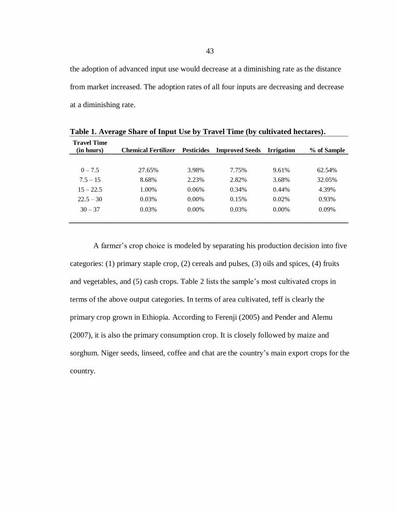
43
the adoption of advanced input use would decrease at a diminishing rate as the distance
from market increased. The adoption rates of all four inputs are decreasing and decrease
at a diminishing rate.
Table 1. Average Share of Input Use by Travel Time (by cultivated hectares).
Travel Time
(in hours)
Chemical Fertilizer Pesticides Improved Seeds Irrigation
% of Sample
0 – 7.5
27.65% 3.98% 7.75% 9.61%
62.54%
7.5 – 15
8.68% 2.23% 2.82% 3.68%
32.05%
15 – 22.5
1.00% 0.06% 0.34% 0.44%
4.39%
22.5 – 30
0.03% 0.00% 0.15% 0.02%
0.93%
30 – 37
0.03% 0.00% 0.03% 0.00%
0.09%
A farmer‘s crop choice is modeled by separating his production decision into five
categories: (1) primary staple crop, (2) cereals and pulses, (3) oils and spices, (4) fruits
and vegetables, and (5) cash crops. Table 2 lists the sample‘s most cultivated crops in
terms of the above output categories. In terms of area cultivated, teff is clearly the
primary crop grown in Ethiopia. According to Ferenji (2005) and Pender and Alemu
(2007), it is also the primary consumption crop. It is closely followed by maize and
sorghum. Niger seeds, linseed, coffee and chat are the country‘s main export crops for the
country.
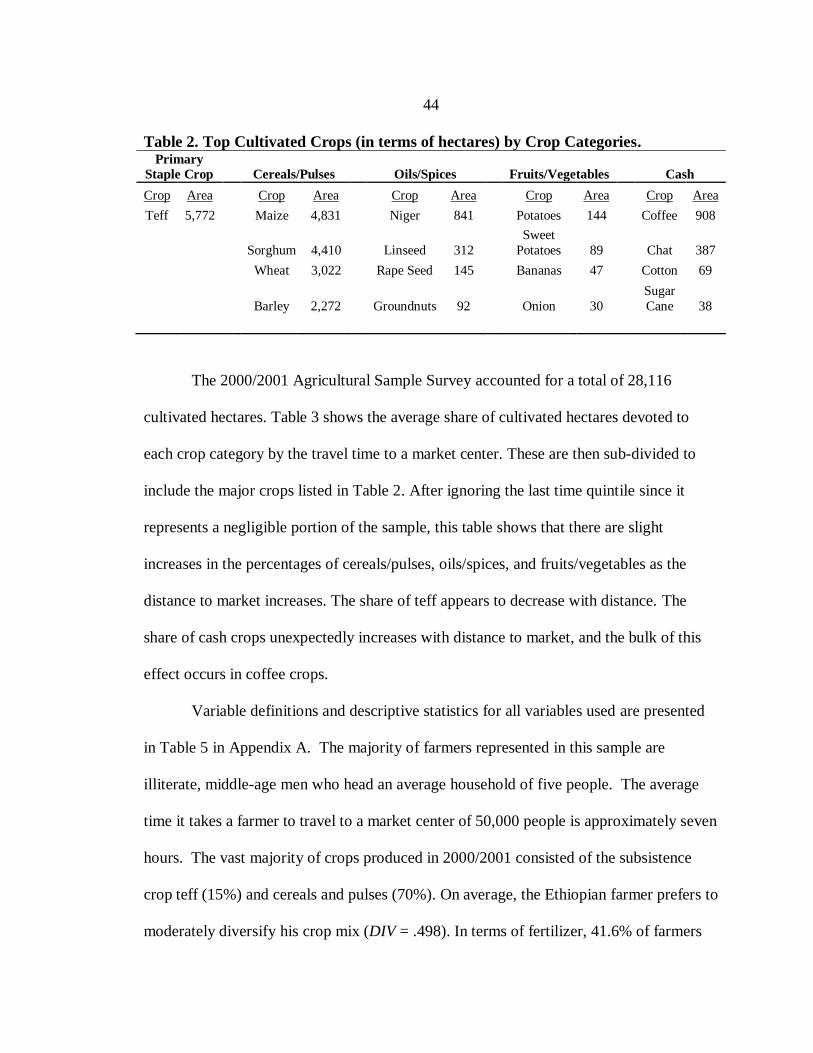
44
Table 2. Top Cultivated Crops (in terms of hectares) by Crop Categories. Primary
Staple Crop
Cereals/Pulses
Oils/Spices
Fruits/Vegetables
Cash
Crop Area
Crop Area
Crop Area
Crop Area
Crop Area
Teff 5,772
Maize 4,831
Niger 841
Potatoes 144
Coffee 908
Sorghum 4,410
Linseed 312
Sweet
Potatoes 89
Chat 387
Wheat 3,022
Rape Seed 145
Bananas 47
Cotton 69
Barley 2,272
Groundnuts 92
Onion 30
Sugar
Cane 38
The 2000/2001 Agricultural Sample Survey accounted for a total of 28,116
cultivated hectares. Table 3 shows the average share of cultivated hectares devoted to
each crop category by the travel time to a market center. These are then sub-divided to
include the major crops listed in Table 2. After ignoring the last time quintile since it
represents a negligible portion of the sample, this table shows that there are slight
increases in the percentages of cereals/pulses, oils/spices, and fruits/vegetables as the
distance to market increases. The share of teff appears to decrease with distance. The
share of cash crops unexpectedly increases with distance to market, and the bulk of this
effect occurs in coffee crops.
Variable definitions and descriptive statistics for all variables used are presented
in Table 5 in Appendix A. The majority of farmers represented in this sample are
illiterate, middle-age men who head an average household of five people. The average
time it takes a farmer to travel to a market center of 50,000 people is approximately seven
hours. The vast majority of crops produced in 2000/2001 consisted of the subsistence
crop teff (15%) and cereals and pulses (70%). On average, the Ethiopian farmer prefers to
moderately diversify his crop mix (DIV = .498). In terms of fertilizer, 41.6% of farmers
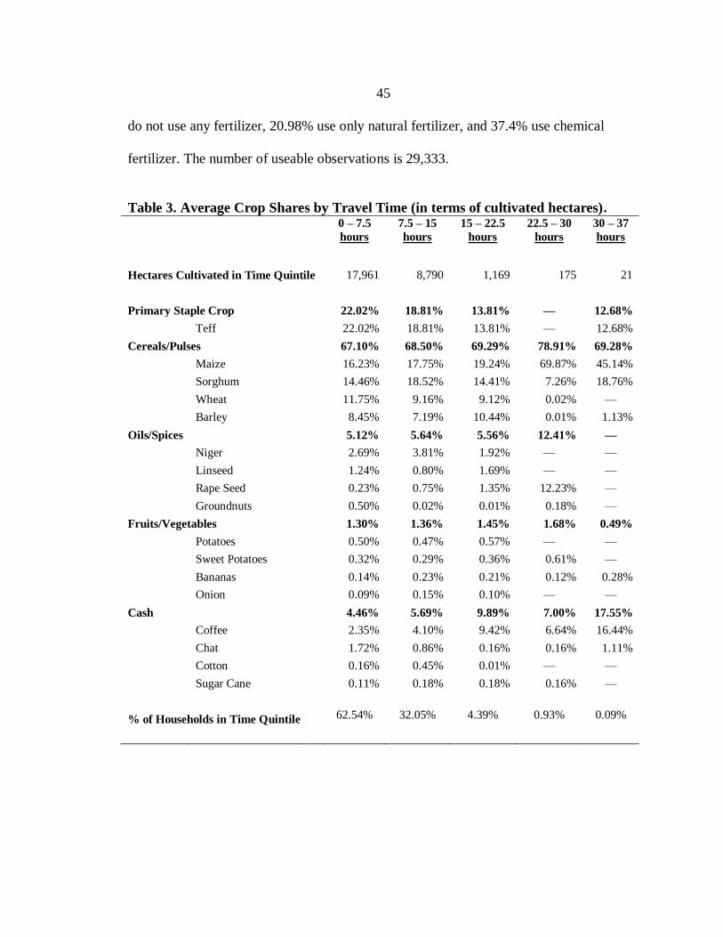
45
do not use any fertilizer, 20.98% use only natural fertilizer, and 37.4% use chemical
fertilizer. The number of useable observations is 29,333.
Table 3. Average Crop Shares by Travel Time (in terms of cultivated hectares).
0 – 7.5
hours
7.5 – 15
hours
15 – 22.5
hours
22.5 – 30
hours
30 – 37
hours
Hectares Cultivated in Time Quintile 17,961 8,790 1,169 175 21
Primary Staple Crop
22.02% 18.81% 13.81% — 12.68%
Teff
22.02% 18.81% 13.81% — 12.68%
Cereals/Pulses
67.10% 68.50% 69.29% 78.91% 69.28%
Maize
16.23% 17.75% 19.24% 69.87% 45.14%
Sorghum
14.46% 18.52% 14.41% 7.26% 18.76%
Wheat
11.75% 9.16% 9.12% 0.02% —
Barley
8.45% 7.19% 10.44% 0.01% 1.13%
Oils/Spices
5.12% 5.64% 5.56% 12.41% —
Niger
2.69% 3.81% 1.92% — —
Linseed
1.24% 0.80% 1.69% — —
Rape Seed
0.23% 0.75% 1.35% 12.23% —
Groundnuts 0.50% 0.02% 0.01% 0.18% —
Fruits/Vegetables
1.30% 1.36% 1.45% 1.68% 0.49%
Potatoes
0.50% 0.47% 0.57% — —
Sweet Potatoes 0.32% 0.29% 0.36% 0.61% —
Bananas
0.14% 0.23% 0.21% 0.12% 0.28%
Onion
0.09% 0.15% 0.10% — —
Cash
4.46% 5.69% 9.89% 7.00% 17.55%
Coffee
2.35% 4.10% 9.42% 6.64% 16.44%
Chat
1.72% 0.86% 0.16% 0.16% 1.11%
Cotton
0.16% 0.45% 0.01% — —
Sugar Cane 0.11% 0.18% 0.18% 0.16% —
% of Households in Time Quintile 62.54% 32.05% 4.39% 0.93% 0.09%

46
CHAPTER 6
CHEMICAL FERTILIZER AND CROP DIVERSIFICATION
A combination of limited dependent models is used to estimate the effects of
market isolation on input use and crop diversification. The analysis of input use is
focused on chemical fertilizer adoption; this variable is modeled both as the household‘s
binary decision to use chemical fertilizer on any field in cultivation and in terms of the
intensity of adoption over the cultivated area. Crop diversification is a measurement of
the number of different crops under cultivation as indicated by the Herfindahl index. It is
possible that the decision to use chemical fertilizer is influenced by a farmer‘s decision to
diversify and vice versa. This potential endogeneity indicates reason to believe that these
two decisions should be modeled simultaneously.
Empirical Models
The decision to use chemical fertilizer is measured both in binary terms and
continuously. Thus, depending on the formation of the variable, the decision is estimated
by using a logit or a Tobit regression. A Tobit regression is used to explain a farmer‘s
decision to diversify his crop mix. The basic econometric models are of the following
forms:
(6.1)
(6.2)
CFERTi is a measure of chemical fertilizer adoption by farmer i,
47
DIVi is equal to the sum of crop shares squared for each crop produced by
farmer i,11
TTIMEi is the average time (in hours) it take to travel to a market center of 50,000
people or greater from the wereda where farmer i resides,
Wi is a vector of the individual farm characteristics held by farmer i,
Xi is a vector of the individual demographic characteristics of farmer i,
Zi is a vector of wereda-specific characteristics that define the wereda where
farmer i resides,
εi is the error term.
Vector W includes variables that characterize the production environment of the
farm. Included are a binary measure of irrigation use and the total area and number of
fields under cultivation by the farmer. The area cultivated and the number of fields are
not used in the diversification model because they are correlated with the Herfindahl
index that measures diversification. The farmer-specific variables included in vector X
are age, sex, education level, and household size.
The variables included in the vector Z represent the bioclimatic and economic
nature of the region where the farmer resides. Biophysical variables are average
elevation, average slope, tree coverage, all-weather road density (meters per km2), and a
measure of rainfall in the wereda. Variables that describe a farmer‘s ability to access
services are population density of the wereda (hundreds of people per km2) and number
of banks, primary schools, and secondary schools present in the wereda. The area of a
11 The measure of crop diversification has a value of 1 when the farmer is completely specializing and
approaches 0 as the number of crops produced by the farmer gets larger.

48
farmer‘s respective wereda is not significantly associated with chemical fertilizer
adoption and is only used to identify diversification practices so as to properly identify
the simultaneous equation model.
Empirical Variable Definitions and Expectations
Wealth effects are modeled by IRR and FARM_AREA, where IRR is a measure of
irrigation use and FARM_AREA is the total size of the farm in cultivation. The high fixed
costs associated with an irrigation system limit the number of investing households.
Larger farm size is also associated with wealth, in terms of production possibilities. Since
land in Ethiopia is nationalized, households do not have the ability to adjust the size of
their land holdings and as a result of this communal process, the range of farm sizes in
Ethiopia is very narrow. Increased wealth gives households more flexibility to bear risk
and allocate financial resources to inputs, therefore, it would be expected that IRR and
FARM_AREA would positively affect both the rate and intensity of chemical fertilizer
adoption. Additionally, wealthier farmers may be more likely to specialize in high value
crops.
Variables that model the ability for a household to access information and markets
are SEX, ED, POPDEN, SEC_SCH, ROADDEN, and TTIME. Males tend to have greater
opportunities to attend school in developing countries, and farmers with higher education
are able to allocate resources more efficiently. Areas of higher population density require
more complex market institutions to facilitate daily interactions. All-weather roads
significantly decrease transaction costs associated with the purchase and transport of
inputs. More secondary schools are developed around areas that require higher skilled
49
workers; areas that would necessitate the need for developed markets. Access to a market
center is hindered by road quality, and geographical conditions such as water bodies and
mountainous regions. TTIME, travel time to a market, takes all of these variables into
consideration. Greater access to markets and information concerning inputs and prices
would predictably be associated with higher propensities to adopt chemical fertilizer. It is
hypothesized that households will choose to grow more specialized and profitable crops
when they have better access to a market, so the relationship to diversification is expected
to be negative.
The AGE of a farmer would capture experience, but the experience of a farmer
does not necessarily affect the propensity of chemical fertilizer adoption or crop
diversification in one direction or another. The effect of HHSIZE, household size, is also
indeterminate in sign. Household size could be a proxy for labor, and thus, more labor
would allow for more intensive chemical fertilizer use or allow for more crops to be
grown at a time (Croppenstedt et al., 2003). Larger households may be using more
chemical fertilizer to increase the output necessary to sustain the family (Nkonya et al.,
1997). A larger household may also want to diversify its crop structure to satisfy a variety
of food preferences. However, it may not be possible for large, poor households to
allocate financial resources to advanced technologies over other necessities (Fufa and
Hassan, 2006). Additionally, larger households may not have the financial resources to
invest in the production of several types of crops.

50
Empirical Methodology
Chemical Fertilizer Regression
Studies of technology adoption model the diffusion of innovation in two ways:
whether or not an individual chooses to use the innovation and/or the intensity of
adoption by an individual. For this analysis, the decision will be modeled both in terms of
whether households used chemical fertilizer in the 2000/2001 farming season, as well as
the degree of fertilizer intensity each household employed as a share of total hectares
cultivated. In the studied time period about 37% of Ethiopian farmers used chemical
fertilizer, and of that group, farmers chose to apply chemical fertilizer to an average of
57% of their farm. Figure 2 displays the distribution of the intensity of chemical fertilizer
use by Ethiopian farmers who have chosen to adopt the input.
As a starting point, OLS was used to examine the variables that affect chemical
fertilizer use, however, the estimates are assumed to be biased because of the nature of
the dependent variable. The construction of the chemical fertilizer adoption variables
limits the values to either a binary decision (yes/no) or a crude measure of fertilizer
intensification as a proportion between zero and one. This limited information is not
appropriately accounted for by conventional regression methods because distributions of
the dependent variable can no longer be assumed to be normal. However, if the decision
is analyzed under the framework of a probability model, the problem is more tractable.
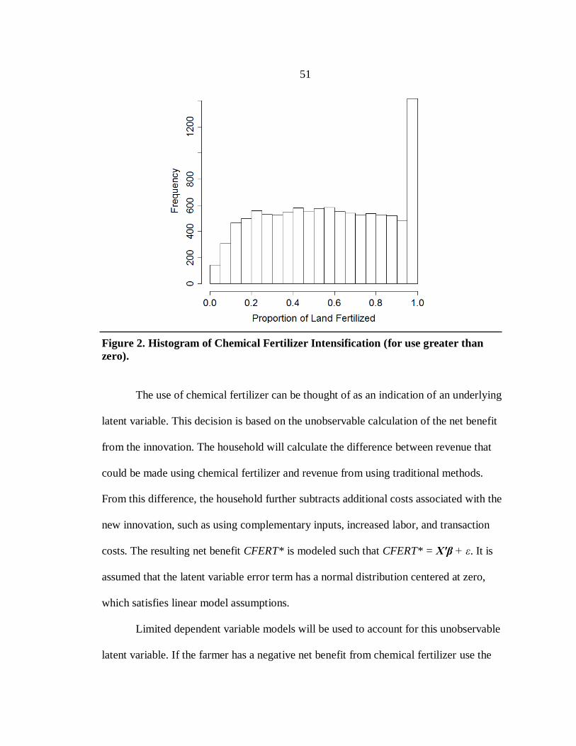
51
Figure 2. Histogram of Chemical Fertilizer Intensification (for use greater than
zero).
The use of chemical fertilizer can be thought of as an indication of an underlying
latent variable. This decision is based on the unobservable calculation of the net benefit
from the innovation. The household will calculate the difference between revenue that
could be made using chemical fertilizer and revenue from using traditional methods.
From this difference, the household further subtracts additional costs associated with the
new innovation, such as using complementary inputs, increased labor, and transaction
costs. The resulting net benefit CFERT* is modeled such that CFERT* = X′β + ε. It is
assumed that the latent variable error term has a normal distribution centered at zero,
which satisfies linear model assumptions.
Limited dependent variable models will be used to account for this unobservable
latent variable. If the farmer has a negative net benefit from chemical fertilizer use the

52
variable is automatically censored at zero. The first method of adoption measurement
answers the question: Did the household use chemical fertilizer on any of its fields? The
answer is translated from the latent variable such that,
(6.3) ,
.
The second method of adoption measurement answers the question: On what percentage
of its operation (in terms of hectares) did the household use chemical fertilizer? The
translation of the latent variable will be continuous and between zero and one,
(6.4) ,
.
The decision to use chemical fertilizer on any fields under cultivation is expressed
as a zero or one variable, such as in equations (6.3), and will be estimated using a binary
choice model. This model relates the probability of choosing to use chemical fertilizer to
a vector of farmer-, farm-, and regional-explanatory variables through the equations:
(6.5) ,
,
where F(·) is the cumulative density function.
The effect of changes in the explanatory variables on the probability of using
chemical fertilizer is reflected through the parameter vector, β. To maintain estimated
probability predictions between 0 and 1 from equations (6.5), a nonlinear model should
be used (Greene, 2008). Assumptions about the distribution of the error term determine
which binary choice model is appropriate. If it is assumed that the error terms are

53
distributed logistically, then a logit model should be used. If the error term is assumed to
be distributed normally, then it is more appropriate to use a probit model. These
distributions have similar bell shapes and are both centered at zero. Empirically, there is
little evidence to justify the choice of one model over the other (Maddala, 1983; Greene,
2008). The logistic distribution has larger tails and is therefore more conducive to larger
samples (because there are more observations in the tails) (Maddala, 1983). For this
reason, a logit regression model is used to estimate the probability of chemical fertilizer
adoption by households.
The probability models in (6.5) are used to form the binary choice regression
model,
(6.6) .
The underlying logistic distribution is,
(6.7) .
The logit model is estimated with maximum likelihood estimation, where the maximum
likelihood estimator β maximizes the log-likelihood function through an iterative process
(Greene, 2008). The log likelihood function is a transformation of the joint probability
density function from equations (6.5),
(6.8) .
The decision to use chemical fertilizer is complicated by the fact that it can be
broken into two parts. The household first chooses whether or not to use any fertilizer. If
the household has decided to use fertilizer, it must then choose either to use natural or
chemical fertilizer. These three separate options have been condensed into a binary

54
variable based solely on chemical fertilizer use. Therefore, it may be the case that there is
some correlation unaccounted for between the unobserved factors within the decision of
what type of fertilizer to use. A nested logit is used to quantify this correlation in the form
of a log sum coefficient λ.12
As λ approaches zero, it indicates that there is perfect
correlation between the unobserved factors within a nest (in this case, the decision about
fertilizer type). If λ is equal to 1 there is no correlation present and the nested logit is
identical to using a standard logit. The OLS, standard logit, and nested logit estimates for
the decision to use chemical fertilizer are presented in Table 6 in Appendix A. The log-
sum coefficient (λ) is equal to 0.037, which would indicate that there is almost perfect
correlation between the unobserved factors affecting the fertilizer type decision. This
necessitates the use of a nested logit model for the examination of chemical fertilizer use
probabilities.
Decisions to use chemical fertilizer are often made simultaneously with other
agricultural innovations, such as pesticides and improved seed (Smale et al., 1994).
Therefore, while the decision to use complementary inputs does affect the probability of
using chemical fertilizer, there is a good chance that the variables are endogenously
determined. A quick comparison of the estimates with and without pesticide and seed use
shows that there does appear to be an endogeneity problem. The standard errors in the
logit regression without pesticides and improved seed are lower than in the regression
with these variables included, and the magnitudes of the estimates are higher. This
endogeneity could be formally tested and accounted for in the context of a 2SLS model,
but the focus of this analysis is on the effects of market access on production decisions,
12 An in depth discussion of the nested logit model is presented in both Greene (2008) and Train (2009).

55
so the complementary inputs have been omitted from the regression on chemical fertilizer
adoption.
The intensity of chemical fertilizer use is expressed as a value from zero to one,
such as in equations (6.4), and will be estimated using the Tobit censored regression
model. All negative net benefit values are observed as zero chemical fertilizer use. The
magnitude of a positive net benefit from chemical fertilizer is transformed into a
percentage based on the amount of hectares fertilized relative to the farm size. The
censored distribution used for the Tobit model is a combination of continuous and
discrete distributions because of the mass of observations at zero. Since the latent
variable has a normal distribution, strictly positive values of CFERT have a continuous
distribution. The probability associated with latent variable values below or equal to the
censoring point is summed to a single, discrete value (Greene, 2008; Wooldridge, 2009).
Following Greene (2008), the resulting expected intensity of chemical fertilizer adoption
derived from the censored distribution is
(6.9) ,
where Φ(·) is the standard cumulative density function, ζ is the standard deviation, and
(·) is the probability density function. The Tobit model works by making the above
mean in (6.9) consistent with conventional regression methods.
The marginal effects from a probability model require a little more attention than
conventional models. In general, the derivative of the binary choice regression model
from equation (6.6) is
(6.10) ,
56
where the traditional derivative is scaled by the probability density function f (·).
In terms of the logistic distribution,
(6.11) .
Thus, the marginal effects of the logit model are
(6.12) .
Greene (2008) presents a formal proof of the marginal effects of a censored Tobit
model. Again, the estimate is multiplied by a scalar (this time by the cumulative density
function):
(6.13) .
Crop Diversification Regression
The variable used to measure crop diversification of Ethiopian households is a
modification of the Herfindahl index of competition that lies strictly between zero and
one. For the same reasons as above, it is not appropriate to use a classical regression
model on this limited dependent variable. The distribution of the diversification measure
is displayed below in Figure 3.
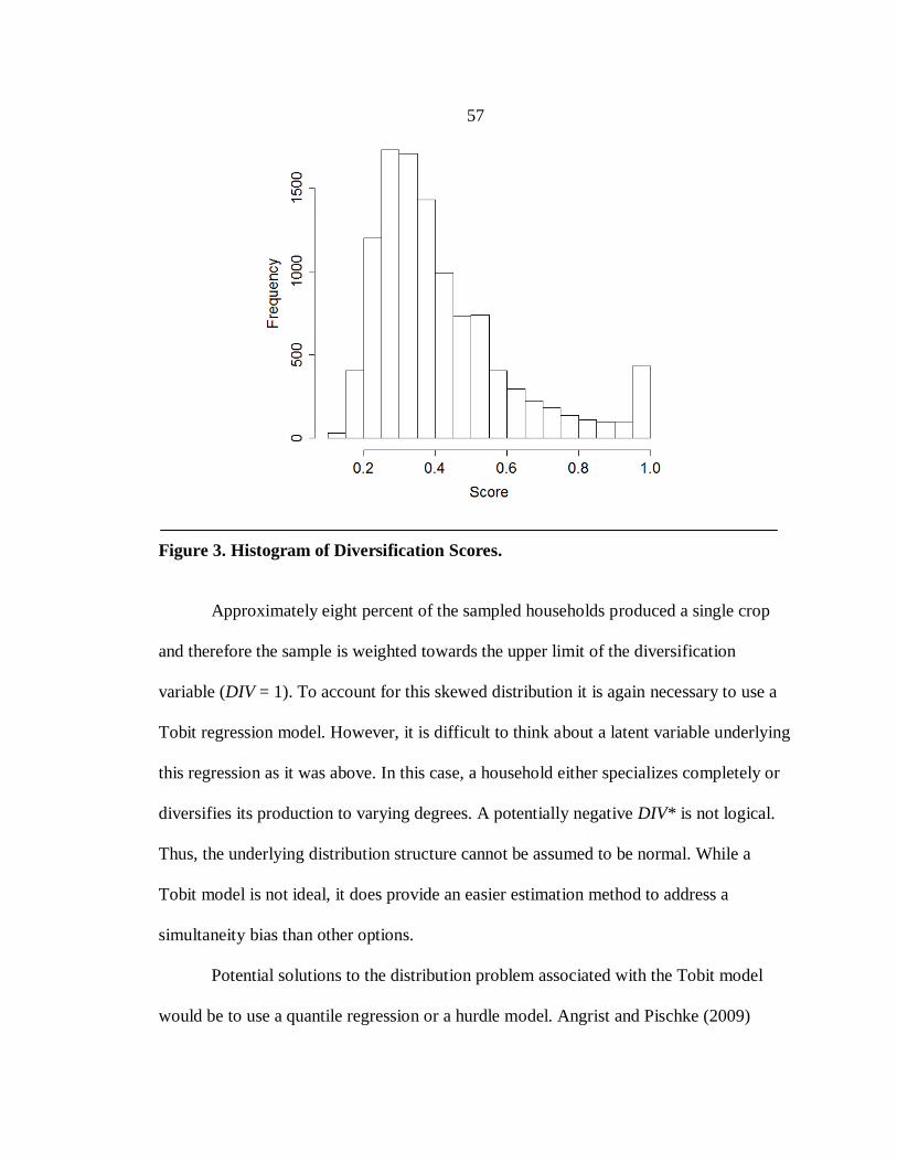
57
Figure 3. Histogram of Diversification Scores.
Approximately eight percent of the sampled households produced a single crop
and therefore the sample is weighted towards the upper limit of the diversification
variable (DIV = 1). To account for this skewed distribution it is again necessary to use a
Tobit regression model. However, it is difficult to think about a latent variable underlying
this regression as it was above. In this case, a household either specializes completely or
diversifies its production to varying degrees. A potentially negative DIV* is not logical.
Thus, the underlying distribution structure cannot be assumed to be normal. While a
Tobit model is not ideal, it does provide an easier estimation method to address a
simultaneity bias than other options.
Potential solutions to the distribution problem associated with the Tobit model
would be to use a quantile regression or a hurdle model. Angrist and Pischke (2009)

58
suggested the use of a quantile regression to examine distribution effects that are not
strictly at the mean. While the Tobit model examines the likelihood of a observing a
value of DIV that is less than or equal to one, a quantile regression model allows for the
analysis of several truncation values, , where c can be equal to any
value between zero and one. A hurdle model assumes that there are two questions being
answered: ―whether or not to diversify‖ and ―how much, given yes.‖ If we treated the
diversification measure as count data we could estimate using a hurdle model and
maximum likelihood. The quantile and hurdle regression models may provide less biased
results, but they are intractable in a simultaneous equation model.
A household‘s decision to use chemical fertilizer or diversify its crop mix is
linked with its decisions about which crops to produce. However, these decisions may be
endogenously connected. Empirical models that included a measurement of crop choice
were estimated and compared to the above models that only include exogenous
regressors; the differences were negligible. The regression results concerning the
intensity of chemical fertilizer use and crop diversification are presented in Table 7 in
Appendix A.
Simultaneous Equation Regression
Due to the expected returns from specializing in certain cash crops like coffee or
chat, the household is generally more inclined to use inputs that produce higher yields.
Thus, each decision variable will be used to explain the other. If chemical fertilizer
adoption and diversification decisions are endogenously determined when they are used

59
as explanatory variables they will be correlated with the error terms, leading to a
simultaneity bias.
A two-stage least squares (2SLS) regression is used to correct for endogenity
through the application of an instrumental variable. Calculating the necessary two-stage
estimates for this analysis requires the use of a simultaneous equation model with two
limited dependent variables. Estimation of a simultaneous equation model using limited
dependent variables is complicated by censoring and the abnormal distributions of the
dependent variables. Nelson and Olsen (1978) proposed a model specification that makes
this problem more tractable. For their example, the authors used a two equation model
with one continuous and one limited dependent variable. In the first stage, the dependent
variables were regressed on all of the exogenous variables using the necessary least
squares or maximum likelihood approaches. In a procedure analogous to the 2SLS
method, the fitted values from the reduced form regressions were used as instrumental
variables in the second stage or the regression as a measurement of the underlying latent
variable. Although Nelson and Olsen only demonstrated their methods using one
continuous variable and one limited dependent variable, they posited that their method
was applicable to a multiple equation simultaneous model with multiple limited
dependent variables. A simulation presented in Appendix B provides compelling
evidence that the proposed two-stage method does return a monotonic transformation of
the underlying latent utility.
Since the dependent variables used in the simultaneous equation model are
limited, it is not possible to approximate a truly unbiased estimate of the underlying

60
utility. However, the simulation suggests that using the fitted values from the first-stage
process to estimate the latent utility, or ‗inclination‘ to perform the action in question
does provide a close approximation when inserted into the second stage of the process.
Although this method has asymptotic properties, the estimates of the underlying utility
from the two-stage simultaneity process will be biased. The degree of bias depends on the
magnitude of censoring. While both measurements of chemical fertilizer are significantly
censored, the intensification of technology adoption, as measured between zero and one,
will be used to determine if a simultaneity bias exists because it contains more
information about the household.
The second stage of the simultaneous system estimation results in a structural
equation. The coefficients on the regressors in this equation must be interpreted carefully
because each regressor affects the dependent variable through two paths: directly,
through the exogenous parameter and indirectly, through the variable‘s effect upon the
model‘s endogenous variables. The fitted values of the endogenous variables only enter
the second stage equation once so, holding all else equal, an inference may be made
about their effect on the dependent variable. However, to make an inference an
assumption must hold. If an omitted variable that affects the fitted values is shocked, it
cannot have an effect on any of the exogenous regressors; this is an unrealistic
assumption. Therefore, it is necessary to express the two equations in their reduced
forms. The results from each stage of the two-stage process and the reduced form
calculations are presented in Table 8 in Appendix A. The differences between the
estimates from the simple Tobit models and the reduced form two-stage models are

61
negligible, which suggest that a simultaneity bias does not exist. The reduced form
estimates, standard errors, and p-values were calculated using a bootstrap method of 1000
draws with replacement. It is intractable, or extremely difficult to know the underlying
distribution of the above limited dependent variables. Bootstrapping is a method that
circumvents this problem and gives more tractable results.
Results
The analysis of results has been separated into three categories: regional-related,
farm-related, and farmer-related characteristics. The above simulation shows that even
though the magnitudes of the estimates are not necessarily an accurate representation of
the underlying utility, the coefficient signs are generally still reliable. Therefore, the
results will be discussed in terms of a household‘s inclination to use chemical fertilizer or
diversify as opposed to a specific degree of behavioral change. Indeed, a comparison
between the Tobit and two-stage reduced form estimates shows that all of the regressors,
except for a couple of variables associated with the insignificant effects of education on
diversification, maintain the same signs throughout.
Regional Characteristics
The main explanatory variable of interest in the above regressions is market
access as measured by the average distance from a wereda to a population center of
50,000 or more. A lack of access to a market for consumption goods could force
smallholders to diversify their crop structure to ensure their dietary needs. Additionally, it
is possible that households closer to market choose to specialize because they have

62
greater access to technologically advanced inputs and are able to purchase subsistence
goods with their higher levels of income. As expected, households further from market
are significantly less likely to adopt chemical fertilizer or diffuse it through their
operation. However, households further from market appear to be less likely to diversify
their crop mixes.
The contradictory result could be explained by the functional form of the model
used or deficiencies in the proxy measure. Perhaps the diversification behavior of
smallholders cannot be modeled in a linear fashion. Households that live close to a
relatively large market center have access to the amenities needed to specialize in high-
value crops. Households that are completely isolated from a market center are
presumably self-sufficient. For environmental and/or financial reasons it may only be
feasible to grow a limited number of crops in more secluded regions. Many smallholders
fall in between these two groups and are likely to produce a portion of their consumption
needs as well as sell their marketed surplus. These households may try to diversify their
crop structures to compensate for the higher degrees of uncertainty associated with
smaller market centers. Therefore, the relationship between diversification and market
access may be more bell-shaped and is difficult to assess using only a single measure of
distance from markets (travel time to a large city). Additionally, the Herfindahl
measurement of diversification is a function of the number of crops grown by a
household, but it does not take into account the value of these crops or the predominance
each crop plays in the household‘s operation.

63
All of the wereda-specific explanatory variables for fertilizer adoption and
diversification are statistically significant in the reduced form models. While biophysical
characteristics of the wereda are likely to affect the feasibility of fertilizer use and crop
growth, their effects are generally difficult to influence with policy changes. The
following analysis of regional characteristics will focus on elements that are of greater
interest to policy makers.
Additional proxies for information and market accessibility are the all-weather
road (m per km2) and population (hundreds of people per km
2) densities of a wereda, as
well as the number of secondary schools in a wereda. Improvements in information and
market accessibility are likely to decrease transaction costs associated with transporting
and buying chemical fertilizer and marketable crops. An increase in the density of all-
weather roads may make it easier to obtain chemical fertilizer, as well as increase the
value of outputs (by decreasing the associated transportation costs). More populated
regions are generally supported by larger market systems. Surprisingly, all-weather road
and population densities are inversely related to chemical fertilizer use. Perhaps the
variables are influenced by smaller household operations closer to urban areas whose
primary focus is not agriculture. As all-weather road and population densities increase,
crop diversification is estimated to decrease; a finding that supports the hypothesis that
households tend to specialize their crop production closer to market. The demand for
secondary education facilities is positively related to the growth of urban areas where
more occupations require higher levels of education. Areas with higher concentrations of
secondary schools will contain more venues for information access. This information aids
64
households as they strive to allocate resources efficiently. As would be expected, both
chemical fertilizer use and crop diversification are predicted to increase with higher
numbers of secondary schools.
The volatile nature of household farming in a developing country necessitates
credit access. Credit allows a household to reduce income risk associated with market and
climatic uncertainty. Credit access for households in the 2000/2001 farming season is
proxied by the number of banks and micro-finance institutions in 2005. According to a
report published by the Ethiopian government in 2002, there were 9 banks with 324
branches in the country (FDRE 2002). The number of branches grew by 16% in 2005 to
378 branches. Since the growth in bank branches mainly took place in urban areas, the
difference in the number of bank branches does not discredit its use as a proxy. However,
having a bank available to a household certainly does not mean that its services are
utilized. It is also more likely that small, low-income production operations will use
micro-finance institutions to access credit. In 2002 there were 19 micro-finance
institutions available to the Ethiopian public; by 2005 this number was in excess of 1,000
(FDRE 2002). Therefore, this may not be the best proxy for the ability to access micro-
finance credit opportunities. According to the data, the probability of chemical fertilizer
use is reduced as the number of banks is increased. This counterintuitive result may be
attributable to the deficiencies in the proxy discussed above. A simple scatter plot reveals
that, all else equal, the number of banks in a wereda is inversely related to the travel time
to a population center of 50,000 or greater. It is likely that households choose to
specialize their crop production in areas closer to a market because they have better

65
access to services such as the sale of high-yielding inputs and credit. Not surprisingly, the
number of banks present in a wereda is estimated to increase a household‘s propensity to
specialize. In terms of micro-financial institutions, an increase in the number of
institutions is estimated to increase the amount of chemical fertilizer used as well as a
household‘s level of diversification.
Farm Characteristics
Choice characteristics concerning the operation of individual farms include
irrigation, the number of fields, and the area cultivated. The decision to use irrigation on
any field in cultivation negatively effects chemical fertilizer use and positively effects
crop specialization. Presumably, the decision to use irrigation would be associated with
the household‘s decisions on crop specialization, because if the infrastructure was already
in place, the smallholder could allocate more of its resources to a smaller number of more
marketable crops. It is estimated that farmer‘s who have the capability to use irrigation
are less likely to use chemical fertilizer. Perhaps, chemical fertilizer and irrigation are
substitute goods in terms of agricultural productivity. If smallholders are able to exert
greater control over their water supplies, they may not feel a need to use as much
chemical fertilizer. One problem that arises with these variables concerns loss of
information from aggregation. Since the data has been summarized at a household level,
it is not possible to know what inputs are generally paired with a particular crop.
An increase in the number of fields and farm size are positively linked to the
intensity of chemical fertilizer use. These results are also supported by the work of

66
Nkonya et al (1997) in Tanzania, and Kebede et al. (1990), Demeke et al. (1998), and
Fufa and Hassan (2006) in Ethiopia.
Household Characteristics
Higher levels of education, relative to illiteracy, are related to positive
probabilities of chemical fertilizer use. Literacy rates and education levels were also
found to positively affect chemical fertilizer use by Croppenstedt et al. (2003), Weir and
Knight (2004), and Fufa and Hassan (2006) in Ethiopia. Other than in the second two
years of primary education and first years of university education, relative to illiteracy,
education does not significantly affect a household‘s decision to diversify.
Problems with Estimation
The major markets in Ethiopia are located in the capital city of Addis Ababa. The
country is designed so that all of the major roadways spoke out from the centrally located
capital city. Thus, if smallholders want to trade with areas across the country they are
first directed through the capital. The measure used for market isolation is the travel time
to a city center of 50,000 people or more. The spoke and axle nature of access in the
country validates the use of the travel time variable as a proxy for market access.
However, the analysis would be strengthened if measurements of travel time to
smaller/larger population centers were accessible. Households that are selling marketed
surpluses of staple foods such as grains and common vegetables are able to participate in
markets that are of a much smaller magnitude than found in these large city centers.

67
Having more complete information on the market structures of Ethiopia would make it
easier to identify behavioral differences between farmers.
The Ethiopian government has spent many resources on the promotion of high-
yielding technology, primarily through the use of extension agencies. In this analysis,
information on household access to the services of an extension program was not
available, which will result in omitted variable bias. Since an extension office would
decrease the effects of incomplete and unreliable information, in essence it would reduce
the effects of remoteness. Therefore, the variables on market access are likely to be
biased upward. Although, more likely than not, this bias would not have an effect on the
signs of the effects. Additionally, it is possible that some of the household observations
represent farmers who are participants in an extension program. Their access to fertilizer
and the price they face are not the same as other households, which would also upwardly
bias the effects of market access.
The measure of diversification used in this analysis is a modified Herfindahl
index that is calculated by summing the squares of the different crop shares on the farm,
in terms of area cultivated. This method of measurement may not accurately capture the
smallholder‘s diversification behavior. Squaring the crop shares places more weight on
the smaller percentages. As such, the diversification index may be misleading since it
does not take the same area of land to grow equitable quantities of different crops (e.g.
oranges and wheat). A more accurate assessment of diversification may be to calculate
the percentage of value each crop adds to production. Alternatively, smallholders who

68
base their production decisions on the need to provide basic sustenance for their families,
may base their diversification decisions on the relative riskiness of each crop.
Several of the variables included in the regression are measured at the mean of the
wereda. However, these variables vary across the district, and therefore, it is possible that
households are misrepresented by the data used. This measurement error could lead to an
attenuation bias. Further measurement error may have taken place during the data
collection process.
Summary
The empirical results imply that crop diversification and chemical fertilizer use are
inversely related, but there is not substantial evidence to suggest that these two variables
endogenously determine one another. Increases in the travel time to a market center are
likely to decrease the intensity of chemical fertilizer adoption and increase the level of
crop specialization. Additionally, while education levels have a positive, statistically
significantly relationship to chemical fertilizer adoption, there does not appear to be a
significant connection between crop diversification and the ability to allocate resources
effectively.

69
CHAPTER 7
CROP CHOICE
To estimate the effects of market isolation on crop choice, the household‘s
production system has been separated into five different crop categories: (1) primary
staple crop, (2) cereals and pulses, (3) oils and spices, (4) fruits and vegetables, and (5)
cash crops. These crop categories were chosen based on similarity in crop type, market
value, and consumption patterns.
Empirical Model
The effects of market isolation on cop choice are modeled as follows:
(7.1) ,
CROP%ij is a vector equal to the share of total cultivated area devoted to crop
category j by farmer i,
TTIMEi is the average time (in hours) it take to travel to a market center of 50,000
people or more from the wereda where farmer i resides,
REVij is the estimated relative revenue per hectare (by region) for the respective
crop category j faced by farmer i,
IRR is a binary measure of irrigation use on a farmer i‘s farm,
Xi is a vector of the individual demographic characteristics of farmer i,
Zi is a vector of wereda-specific characteristics that define the wereda where
farmer i resides,
εi is an error term.

70
Farmer-specific variables included in vector X include age, sex, education level,
and household size. Vector Z variables represent the bioclimatic and economic nature of
the region where the farmer resides. Biophysical variables are wereda area, average
elevation, average slope, tree coverage, road density, and a measure of rainfall in the
wereda. Variables that describe a farmer‘s ability to access services are the population
density of the wereda and the number of banks, micro-finance institutions, primary
schools, and secondary schools present in the wereda.
Empirical Variable Definitions and Expectations
The relative revenue variables (REV) used in the regression system were
calculated by dividing a measure of revenue for a single crop category by the average of
revenue estimates of all categories. The revenue measures are significantly correlated, so
singular value decomposition was used to determine which revenue estimates would be
the best to include for empirical reasons. Two revenue estimates located on opposite sides
of the continuum of profitability should be included for economic reasons. Under those
criteria, the best fitting revenue variables were for cereals/pulses and fruits/vegetables. A
measure of revenue was included in the regression system to give a proxy for
profitability. While the revenue variable should positively affect own-crop categories, the
effect of revenue on other crop categories is indeterminate because it is not known which
crop categories are substitutes or complements for each other.
Additional regressors included in the system of OLS equations are included for
reasons similar to the chemical fertilizer and crop diversification models. SEX, ED,
POPDEN, SEC_SCH, ROADDEN, and TTIME all measure the ability of a household to
71
access information and markets. Therefore, more marketable crops would predictably be
positively affected by market access and vice versa for subsistence crops. FARM_AREA,
total cultivated area, is a proxy for the wealth of the household. Higher levels of wealth
are associated with more risky behavior. Households that can afford to feed themselves
will be able to devote more of their resources to income-related activities, such as the
cultivation of cash crops. The effects of input use will vary across crop categories,
depending on the nature of the crops and the financial situation of the household. Again,
household size will be indeterminate in sign. If HHSIZE is a proxy for labor, perhaps
larger households will grow more labor intensive crops. Cash crops may be considered
labor intensive, but the opportunity costs of living near a market area may promote hired
labor off the farm. It is also possible that larger households in a subsistence situation may
be required to grow large amounts of low valued crops, while smaller households have
the freedom to vary their diets and raise cash crops.
Empirical Methodology
Since the five dependent variables in the shares equation sum to one, the five
equations should be modeled as a system. While the disturbances in the error terms are
assumed to uncorrelated across observations, they are inherently correlated across
equations. Following Greene (2008),
(7.2) , if t = s and 0 otherwise.
Therefore, the disturbance formulation is,

72
(7.3)
To account for the error term correlation, a seemingly unrelated model is
estimated using generalized least squares. In terms of efficiency, generalized least
squares is preferred to equation by equation ordinary least squares estimation if the
equations are truly related ( for i ≠ j) and/or the equations do not have identical
regressors (Xi ≠ Xj).
The model in (7.1) contains identical regressors and is thus estimated with
equation by equation OLS. However, because the dependent variables are crop shares,
cross-equation restrictions need to be included. The issue is illustrated in the following
example:
(7.4) ,
,
.
Since the dependent variables are shares, if follows that,
(7.5) = 1
and
.
Therefore, since the three equations are related, the effects of a shock to an explanatory
variable must sum to zero across the equations while the intercepts must sum to one, that
is,

73
(7.6) ,
.
The addition of cross-equation constraints makes it possible to fully identify the
five share equations in a seemingly unrelated system. However, since the sample size is
so large, it is difficult to invert a matrix of the required magnitude. A solution to this
problem would be to break the matrix into manageable subparts, but this will be left for
future research. Instead, it is noted that estimating each individual equation with OLS still
maintains the necessary cross-equation restrictions. The OLS results are presented in
Table 9 in Appendix A.
Although each equation in the system was estimated individually, the marginal
effects of each regressor are interconnected by the crop shares. If an average household
decides to increase its share of cereal and pulse crops it must decrease its shares of the
other four crops simultaneously. Thus, an individual marginal effect can only be
considered relative to the sum of marginal effects in the other four categories.
Spatial Correlation
A major concern with using a country-wide representative dataset arises in the
form of spatial correlation. Failing to control for regional differences can result in
unreliable estimates. To address the issue of spatial correlation, the average OLS
residuals by zones were first plotted on the Ethiopia map to see if there was any visual
evidence of spatial correlation. Two maps for each of the five crop categories are
displayed in Figures 4-8 in Appendix A. The first is a map of the negative versus positive
OLS residuals; the second map uses a color continuum to display the degree of variation

74
(where lighter shades of the color represent residuals closer to 0). All ten maps show
large instances of residual clustering which demonstrates spatial correlation. However,
only a limited amount of information is conveyed by mapping the average residuals,
especially at such a broad district level.
To account for the differences associated with smaller clusters of individuals, a
more accurate assessment can be accomplished using a simulation. Since this is only a
cross-sectional sample, 5,000 observations from each zone were randomly selected with
replacement to form a base measure of spatial relations. Each zonal base measure was
then compared to the other 45 zones through the use of a correlation matrix. The largest
correlation in this matrix was 0.04, which indicates that spatial correlation is not a
substantial problem. Additionally, the variables appear to be independently and
identically distributed when various ranks of the residual matrix were mapped against one
another.
Results
Again, the results will be analyzed in terms of regional-, farm-, and farmer-related
characteristics. Additionally, the estimates will be discussed in terms of the direction, not
magnitude, since the cross-equation correlation of the error term may be accounted for
inaccurately.
Regional Characteristics
Variables that measure the effects of market isolation are TTIME, ROADDEN,
POPDEN, and SEC_SCHL. It was hypothesized that more marketable crops, such as cash

75
crops and oils/spices, will be grown closer to market centers while subsistence oriented
crops like grains and pulses are likely to be produced in areas that are more isolated from
a market because of their associated transaction costs.
In terms of all-weather road density, the shares of cash crops, fruits, and
vegetables are positively affected by higher levels of infrastructure. Cash crops are high-
value crops that are not often consumed by Ethiopian smallholders, thus, it is logical for
these crops to be grown close to a market system to access high-yielding inputs and lower
transaction costs. Fruits and vegetables are also high-value crops that need to be
consumed shortly after harvest. Cereals and pulses are low-value crops that are much
easier to store and prevalent in the Ethiopian diet. Oils and spices are negatively affected
by road density. Although valuable for export, these crops are generally easy to store and
are utilized by Ethiopians in their everyday cooking.
Population density is much higher in the highlands of Ethiopia which has cooler,
more temperate areas. The agro-ecological characteristics of these areas are especially
conducive to the production of cash crops, fruits and vegetables, and cereal crops such as
wheat and barley. Teff is primarily grown in the highlands, but is a major crop in the
highly elevated central and northern highlands which are relatively less densely
populated than the eastern and southern highlands. Cash crops, fruits, vegetables, cereals,
and pulses are positively affected by population density, while there is a negative effect
on teff, oils, and spices. Higher numbers of secondary schools are also distributed
amongst the highland areas of the country. An increase in the number of secondary

76
schools is negatively related to the production share of teff and other cereals and grains,
and positively related to the shares of market-oriented crops.
Increases in the travel time to a population center of 50,000 negatively affect the
shares of teff, oils, spices, and cash crop production and have positive effects on the
shares of cereals, fruits, and vegetables. Although teff is a cereal grain, it is a reliable and
low-risk crop that can be grown in a variety of environments and is a major dietary staple
(Ketema, 1987). Teff is also more profitable relative to other crops, such as wheat and
maize. Its high-value and low risk may explain why production shares of the crop
increase with population density. The share of fruits and vegetables is positively affected
by travel time. Fruits and vegetables can be grown in the majority of the highland areas
of Ethiopia and provide significant nutritional value. Hence, more isolated households
may need to allocate land to these crops because they are not reliably available in the
market place. In addition, the travel time measure of isolation is based on population
centers of 50,000 people or more. Many smaller population centers are based in the
Ethiopian highlands. Thus, the travel time variable may not be an accurate measure of
market access.
Access to credit is measured by the number of banks and micro-finance
institutions in a wereda. Households are more likely to obtain credit for crops with a
higher return on investment. Teff is one of the most common cereals sold on the market
and has a higher price than comparable grains. The number of banks branches in a
wereda is positively related to the production shares of teff, oils, spices, and cash crops.
Micro-finance institutions have developed in the rural areas to provide credit to the

77
subsistence households and promote growth through small loans. The share of cereal
crops is positively affected by micro-finance institutions, but the number of micro-
finance institutions does not significantly affect the share of teff grown.
Farm Characteristics
Irrigation is a permanent asset that is initially financially intensive. It is an
investment that is likely to be associated with high-value crops. Production shares of cash
crops, fruits, vegetables, and teff are positively affected by irrigation use.
Farmer Characteristics
The ability to access and process information on farm efficiency and productivity
is important to maximize household utility. Sex and education levels are included as
proxies for this ability. The regression results indicate that males are less likely to grow
cereals/pulses, fruits/vegetables, and cash crops relative to growing teff, oils, and spices.
In terms of education, as farmers become more educated, relative to illiteracy, they are
more likely to transition from growing cereals and pulses to fruits, vegetables, and cash
crops. These effects could also reflect the fact that people with higher education levels
generally migrate to more urban areas. Increases in household size have a statistically
significant effect on the production shares of teff, cereals/pulses, fruits/vegetables, and
cash crops. It is estimated that larger households generally tend to grow teff and
cereals/pulses over market-oriented crops, such as fruit/vegetables and cash crops.

78
Problems with Estimation
Using a least squares regression method allows for negative fitted values which
does not parallel the nature of the dependent variables. Several of these crop categories
have mass points at zero and/or one. Therefore, it may be more reasonable to use a
limited dependent variable model instead of OLS. In this case, the underlying latent
variable can be thought of as the net benefit of the entire production system. Each
household weighs the costs and benefits of producing various crops before choosing their
ultimate crop mix. Zero production levels of a certain crop category are quite common in
this dataset. Thus, a Tobit model is used to estimate the five equations and the results are
presented in Table 10 in Appendix A. All of the crop category equations are estimated
with a double censored (at zero and one) Tobit model except for fruits and vegetables.
There are some changes in parameter signs and significance between the OLS and
Tobit estimates; these changes are generally consistent between the two measures of
input use. However, one limitation of the Tobit model is the inability to apply cross-
equation restrictions. A future research project could include an attempt to use a
constrained SUR model with Tobit equations. A comparison of the two types of teff
classification shows similar differences to those between the OLS estimates. The
classification of teff does not affect the effects of market isolation on crop choice.
Summary
The empirical results suggest that higher levels of market access do increase the
allocation of land to high value crops. Additionally, as smallholders become more

79
educated and experienced they are more likely to shift their production system away from
subsistence-oriented crops such as cereals and pulses, and transition into the production
of more market-oriented crops.

80
CHAPTER 8
CONCLUSION
Many resources are directed to improving infrastructures and changing
institutions in Ethiopia. Several empirical studies have examined Ethiopia‘s agricultural
sector; research has generally been focused on a handful of major crops in a particular
area. This paper contributes to the literature by utilizing information about smallholders‘
entire farming operations. The empirical work allows for the investigation of tradeoffs
between producing several different types of crops, and examines how these tradeoffs are
affected by market isolation and the smallholder‘s ability to allocate resources efficiently.
The empirical results suggest that smallholders do react to changes in the level of
market access by altering their production behavior. The intensity of chemical fertilizer
adoption decreases and levels of specialization increase as farmers become more isolated
from markets. As travel time to a market decreases, smallholders are also more likely to
allocate land to higher value crops such as cash crops, teff, oils, and spices. With the
exception of the effect of travel time on diversification, these findings are consistent with
the findings reported in previous studies.
In this study, smallholder‘s ability to allocate resources efficiently is proxied by
education levels. Those with some education are likely to use higher levels of chemical
fertilizer than illiterate smallholders. The degree of chemical fertilizer use intensifies as
farmers obtain more years of education. Additionally, as smallholders acquire more
education they tend to allocate their land away from subsistence-oriented crops such as
cereals and pulses, and transition into the production of more market-oriented crops.

81
Travel time to a market center is measured as travel time to a population center of
50,000 or greater. However, effective markets also exist at centers with smaller
population levels, and information about travel time to these centers would help to better
classify smallholders market access. Another limitation of the data is the absence of
information on access to an agricultural extension agency. Much of the government‘s
policy reforms on agriculture are promoted by extension agencies and they play an
integral part in the production decision process. Finally, a household‘s willingness to
adopt new technologies is likely to depend on their ability to access credit. Rates of
micro-finance lending in Ethiopia have increased substantially over the past several
years. Micro-finance institutions were almost non-existent in 2002 and by 2005 there
were over 1,000 different institutions lending to low-income households in the country
(FDRE 2002). An important issue for further research is to examine the effects of micro-
finance lending on advanced technology adoption.
In conclusion, the empirical evidence implies that there are statistically significant
relationships between market isolation and chemical fertilizer adoption, crop
diversification, and crop choice. The results would suggest that economic growth policies
targeted to improve infrastructure, education, and market incentives could potentially
increase the use of technologically advanced inputs, such as chemical fertilizer, and
change the structure of crop diversity towards more market-oriented crop choices.

82
REFERENCES CITED
83
Aiginer, K. (1987). Production and Decision Theory under Uncertainty. New York: Basil
Blackwell.
Alchian, A & Allen, W. (1964). University Economics: Elements of Inquiry. Belmont,
California: Wadsworth.
Alemu, D., Mwangi, W., Nigussie, M., & Spielman, D. (2008). The Maize Seed System
in Ethiopia: Challenges and Opportunities in Drought Prone Areas. African
Journal of Agricultural Research, 3 (4), 305-314.
Anderson, J., Dillion, J., & Hardaker, B. (1977). Agricultural Decision Analysis. Ames,
Iowa: Iowa State University Press.
Angrist, J. D. & Pischke, J. S. (2009). Mostly Harmless Econometrics: An Empiricist’s
Companion. Princeton: Princeton University Press.
Beattie, B. R., Taylor, C. R., & Watts, M. J. (2009). The Economics of Production (2nd
Edition). Malabar, Flordia: Krieger Publishing Company.
Bellon, M. & Taylor, J. E. (1993). ―Folk‖ Soil Taxonomy and the Partial Adoption of
New Seed Varieties. Economic Development and Cultural Change, 41 (4), 763-
786.
Binswanger, H. & Von Braun, J. (1991). Technological Change and Commercialization
in Agriculture: The Effect on the Poor. The World Bank Research Observer, 6 (1),
57-80.
von Braun, J. (1995). Agricultural Commercialization: Impacts on Income and Nutrition
and Implications for Policy. Food Policy, 20 (3), 187-202.
Byerlee, D., & Hesse de Polanco, E. (1986). Farmers' Stepwise Adoption of
Technological Packages: Evidence from the Mexican Altiplano. American
Journal of Agricultural Economics , 68 (3), 519-527.
Byerlee, D., Speilman, D., Alemu, D., & Gautam, Madhur. (2007). Policies to Promote
Cereal Intensification in Ethiopia: A Review of Evidence and Experience. IFPRI
Discussion Paper 00707, International Food Policy Research Institute.
CSA & IFPRI. (2006). Atlas of the Ethiopian Rural Economy. Published by the Central
Statistical Agency, Federal Democratic Republic of Ethiopia and International
Food Policy Research Institute, Washington, DC, USA.
Central Statistical Agency of Ethiopia. (2007). Agricultural Sample Survey (AgSS2000),
Version 1.1.
84
Central Stastical Agency of Ethiopia. Consumer Price Database. (Survey 1 [1989-
1993]). Retrieved October 2009.
<http://www.csa.gov.et/index.php?option=com_wrapper&view=wrapper&Itemid
=113>.
Chambers, R. G. & Quiggin, J. (2000). Uncertainty, Production, Choice, and Agency.
New York: Cambridge University Press.
Coxhead, I. & Warr, P. (1991). Technical Change, Land Quality, and Income
Distribution: A General Equilibrium Analysis. American Journal of Agricultural
Economics, 73 (2), 345-360.
Croppenstedt, A. & Demeke, M. (1996). Determinants of Adoption and Levels of
Demand for Fertilizer for Cereal Growing Farmers in Ethiopia. Centre for the
Study of African Economies Working Paper WPS/96-3 (University of Oxford).
Croppenstedt, A., Demeke, M., & Meschi, M. M. (2003). Technology Adoption in the
Presence of Constraints: the Case of Fertilizer Demand in Ethiopia. Review of
Development Economics , 7 (1), 58-70.
Debertin, D. (2002). Agricultural Production Economics (2nd
Edition). University of
Kentucky. Retrieved October 2009. <
http://www.uky.edu/~deberti/prod/AgprodCD2007>.
Demeke, M., Said, A., & Jayne, T. S. (1997). Promoting Fertilizer Use in Ethiopia: The
Implication of Improving Grain Market Performance, Input Market Efficiency
and Farm Management. Grain Market Research Project, Working Paper 5,
Ministry of Economic Development and Cooperation, Ethiopia.
Demeke, M., Said, A., & Jayne, T. S. (1998). Agricultural Market Performance and
Determinants of Fertilizer Use in Ethiopia. Grain Market Research Project,
Working Paper 10, Ministry of Economic Development and Cooperation,
Ethiopia.
Diamond, J. (2005). Guns, Germs, and Steel. W. W. Norton and Company: New York.
Dillon, J. & Scandizzo, P. L. (1978). Risk Attitudes of Subsistence Farmers in Northeast
Brazil: A Sampling Approach. American Journal of Agricultural Economics, 60
(3), 425-435.
European Communities. (2008). Travel Time to Major Cities: A Global Map of
Accessibility. Created by the European Commission and World Bank. Retrieved
on October 2009. <http://bioval.jrc.ec.europa.eu/products/gam/>.
85
Fafchamps, M. (1992). Cash Crop Production, Food Price Volatility, and Rural Market
Integration in the Third World. American Journal of Agricultural Economics , 74
(1), 90-99.
Fafchamps, M. & Shilpi, F. (2003). The Spatial Division of Labour in Nepal. The Journal
of Development Studies , 39 (6), 23-66.
Feder, G. (1980). Farm Size, Risk Aversion, and the Adoption of New Technology under
Uncertainty. Oxford Economic Papers, 32 (2), 263-283.
Feder, G., Just, R., & Zilberman, D. (1985). Adoption of Agricultural Innovations in
Developing Countries: A Survey. Economic Development and Cultural Change,
33 (2), 255-298.
Federal Democratic Republic of Ethiopia. (July 2002). Ethiopia: Sustainable
Development and Poverty Reduction Program. A Report by the Ministry of
Finance and Economic Development, Addis Ababa, Ethiopia.
Ferenji, B. T. (2005). The Impact of Policy Reform and Institutional Transformation on
Agricultural Performance: An Economic Study of Ethiopian Agriculture.
Frankfurt: Peter Lang.
Finkelshtain, I. & Chalfant, J. A. (1991). Marketed Surplus under Risk: Do Peasants
Agree with Sandmo? American Journal of Agricultural Economics, 73 (3), 557-
567.
Fufa, B. & Hassan, R. (2006). Determinants of Fertilizer Use on Maize in Eastern
Ethiopia: A weighted Endogenous Sampling Analysis of the Extent and Intensity
of Adoption. Agrekon , 45 (1), 38-48.
Goetz, S. (1992). A Selectivity Model of Household Food Marketing Behavior in Sub-
Saharan Africa. American Journal of Agricultural Economics, 74 (2), 444-452.
Green, D. A. G. & Ng'ong'ola, D. H. (1993). Factors Affecting Fertilizer Adoption in
Less Developed Countries: An Application of Multivariate Logistic Analysis in
Malawi. Journal of Agricultural Economics, 44 (1), 99-109.
Greene, W. H. (2008). Econometric Analysis (6th
Edition). New Jersey: Pearson Hall.
Griliches, Z. (1957). Hybrid Corn: An Exploration in the Economies of Technological
Change. Econometrica, 25 (4), 501-522.
86
Hayami, Y. & Herdt, R. (1977). Market Price Effects of Technological Change on
Income Distribution in Semisubsistence Agriculture. American Journal of
Agricultural Economics, 59 (2), 245-256.
Heady, E. & Dillon, J. (1952). Agricultural Production Functions. Ames, IA: Iowa State
University Press.
Hirshleifer, J., Glazer, A., & Hirshleifer, D. (2005). Price Theory and Applications (7th
Edition). Cambridge: Cambridge University Press.
Holden, S. T., Taylor, J. E., & Hampton, S. (1998). Structural Adjustment and Market
Imperfections: A Stylized Village Economy-Wide Model with Non-Separable
Farm Households. Environment and Development Economics , 4, 69-87.
Iqbal, F. (1986). The Demand and Supply of Funds among Agricultural Households in
India. Agricultural Household Models: Extensions, Applications and Policy.
Singh, I., Squire, L., Strauss, J., (ed.). A World Bank Publication. Baltimore:
Johns Hopkins University Press.
de Janvry, A., Fafchamps, M., & Sadoulet, E. (1991). Peasant Household Behaviour with
Missing Markets: Some Paradoxes Explained. The Economic Journal , 101, 1400-
1417.
Jayne, T. S., Negassa, A., & Myers, R. (1998). The Effect of Liberalization on Grain
Prices and Marketing Margins in Ethiopia. MSU International Development
Working Paper No. 68, Michigan State University, East Lansing.
Just, R. E. & Zilberman, D. (1983). Stochastic Structure, Farm Size and Technology
Adoption in Developing Agriculture. Oxford Economic Papers, Oxford
University Press, 35 (2), 307-328.
Kamara, A. B. (2004). The Impact of Market Access of Input Use and Agricultural
Productivity: Evidence from Machakos District, Kenya. Journal of Agriculture
and Food Science , 2 (2), 77-90.
Kebede, Y., Gunjal, K., & Coffin, G. (1990). Adoption of New Technologies in
Ethiopian Agriculture: The Case of Tegulet-Bulga District Shoa Province.
Agricultural Economics, 4 (1), 27-43.
Ketema, S. (1987). Research Recommendations for Production and Brief Outline of
Strategy for the Improvement of Tef [Eragrostis Tef (Zucc.) Trotter]. Proceedings
of the 19th National Crop Improvement Conference, Addis Ababa, Ethiopia, 140-
151.

87
Key, N., Sadoulet, E., & de Janvry, A. (2000). Transactions Costs and Agricultural
Household Supply Response. American Journal of Agricultural Economics, 82
(2), 245-259.
Lekvall, P. & Wahlbin, C. (1973). A Study of Some Assumptions Underlying Innovation
Diffusion Functions. Swedish Journal of Economics, 75 (4), 362-377.
Maddala, G. S. (1983). Limited-Dependent and Qualitative Variables in Econometrics.
Cambridge: Cambridge University Press.
Mansfied, E. (1963). The Speed of Response of Firms to New Techniques. Quarterly
Journal of Economics, 77 (2), 290-311.
Moschini, G. & Hennessy, D. A. (2001). Uncertainty, Risk Aversion, and Risk
Management for Agricultural Producers. Handbook of Agricultural Economics
(1st Edition, Volume 1, Chapter 2), Gardner, B. L., & Rausser, G. C. (ed.),
Amsterdam: Elsevier, 88-153.
Negassa, A., & Jayne, T. S. (1998). The Response of Ethiopian Grain Markets to
Liberalization. Grain Market Research Project, Working Paper 10, Ministry of
Economic Development and Cooperation, Ethiopia.
Nelson, F. & Olson, L. (1978). Specification and Estimation of a Simultaneous-Equation
Model with Limited Dependent Variables. International Economic Review , 19
(3), 695-709.
Nkonya, E., Schroeder, T., & Norman, D. (1997). Factors Affecting Adoption Of
Improved Maize Seed And Fertilizer In Northern Tanzania. Journal of
Agricultural Economics, 48 (1-3), 1-12.
Omamo, S. (1998a). Transport Costs and Smallholder Cropping Choices: An Application
to Siaya District, Kenya. American Journal of Agricultural Economics , 80 (2),
116-123.
__________. (1998b). Farm-to-Market Transaction Costs and Specialization in Small-
Scale Agriculture: Explorations with a Non-Separable Household Model. The
Journal of Development Studies , 35 (2), 152-163.
Pender, J. & Alemu, D. (2007). Determinants of smallholder commercialization of food
crops: Theory and evidence from Ethiopia. IFPRI discussion papers 745,
International Food Policy Research Institute (IFPRI).
Pingali, P. L. & Rosegrant, M. W. (1995). Agricultrual Commercialization and
Diversification: Process and Polices. Food Policy , 20 (3), 171-185.
88
Renkow, M. (1990). Household Inventories and Marketed Surplus in Semisubsistence
Agriculture. American Journal of Agricultural Economics, 72 (3), 664-675.
__________. (1993). Differential Technology Adoption and Income Distribution in
Pakistan: Implications for Research Allocation. American Journal of Agricultural
Economics, 75 (1), 33-43.
__________. (1994). Technology, Production Environment, and Household Income:
Assessing the Regional Impacts of Technological Change. Agricultural
Economics, 10 (3), 219-231.
Renkow, M., Hallstrom, D., & Karanja, D. (2003). Rural Infrastructure, Transactions
Costs and Market Participation in Kenya. Journal of Development Economics,73
(1), 349– 367.
Roe, T. & Graham-Tomasi, T. (1986). Yield Risk in a Dynamic Model of the
Agricultural Household. Agricultural Household Models: Extensions,
Applications and Policy, Singh, I., Squire, L., Strauss, J., (ed.). A World Bank
Publication. Baltimore: Johns Hopkins University Press.
Rogers, E. M. (1995). Diffusion of Innovations (Forth Edition). New York: The Free
Press.
Sandmo, A. (1971). On the Theory of the Competitive Firm under Price Uncertainty.
American Economic Review, 61 (1), 65-73.
Scobie, G. & Posada, T. (1978). The Impact of Technical Change on Income
Distribution: The Case of Rice in Colombia. American Journal of Agricultural
Economics, 60 (1), 85-92.
Singh, I., Squire, L., & Strauss, J., (ed.). (1986). Agricultural Household Models:
Extensions, Applications and Policy. A World Bank Publication. Baltimore: Johns
Hopkins University Press.
Stepanek, J. (1999). Lessons from Ethiopia‘s High-Input Technology Promotion
Program: How the Organization of the Fertilizer Subsector Affects Maize
Productivity. PhD dissertation, Michigan State University, East Lansing.
Stifel, D. & Minton, B. (2004). Isolation, Welfare, and Agricultural Productivity. Cornell
University Working Paper.
Strauss, J. (1984). Marketed Surpluses of Agricultural Households in Sierra Leone.
American Journal of Agricultural Economics, 66 (3), 321-331.

89
Sunding, D. & Zilberman, D. (2001). The Agricultural Innovation Process: Research and
Technology Adoption in a Changing Agricultural Sector. Handbook of
Agricultural Economics (1st Edition, Volume 1, Chapter 4), Gardner, B. L., &
Rausser, G. C. (ed.), Amsterdam: Elsevier, 88-153.
Sutherland, J. (2002). Support for Fertilizer Market Development in Ethiopia. Ethiopia
National Fertilizer Sector Project, World Bank.
Taylor, J. & Adelman, I. (2003). Agricultural Household Models: Genesis, Evolution,
and Extensions. Review of Economics of the Household, 1(1), 33-58.
Thapa, G., Otsuka, K., & Barker, R. (1992). Effect of Modern Rice Varieties and
Irrigation on Household Income Distribution in Nepalese Villages. Agricultural
Economics, 7 (3-4), 245-265.
von Thünen, J. H. (1966). Von Thünen's Isolated State. (P. Hall, Ed., & C. M.
Wartenberg, Trans.) New York: Pergamon Press Ltd.
Train, K. E. (2009). Discrete Choice Methods with Simulation (2nd Edition). New York:
Cambridge University Press.
Vakis, R., Sadoulet, E., & de Janvry, A. (2003). Measuring Transactions Costs from
Observed Behavior: Market Choices in Peru. Department of Agricultural and
Resource Economics, UC Berkeley, Working Paper Series 962, Department of
Agricultural & Resource Economics, UC Berkeley.
Visser, S. (1980). Technological Change and the Spatial Structure of Agriculture.
Economic Geography, 56 (4), 311-319.
Weir, S. & Knight, J. (2004). Externality Effects of Education: Dynamics of the Adoption
and Diffusion of an Innovation in Rural Ethiopia. Economic Development and
Cultural Change , 53, 93-113.
World Bank. (2005). Well-Being and Poverty in Ethiopia: The Role of Agriculture and
Agency. Report No. 29468-ET. Poverty Reduction and Economic Management 2
(AFTP2), County Department for Ethiopia, Africa Region.
Wooldridge, J. (2009). Introductory Econometrics (4th Edition). Mason, OH: South-
Western Cengage Learning.
Wozniak, G. (1987). Human Capital, Information, and the Early Adoption of New
Technology. The Journal of Human Resources, 22 (1), 101-112.

90
Zeller, M., Diagne, A., & Mataya, C. (1997). Market Access by SmallholderFarmers in
Malawi: Implications for Technology Adoption, Agricultural Productivity, and
Crop Income. FCND Discussion Paper No. 35.

91
APPENDICES

92
APPENDIX A
TABLES AND FIGURES
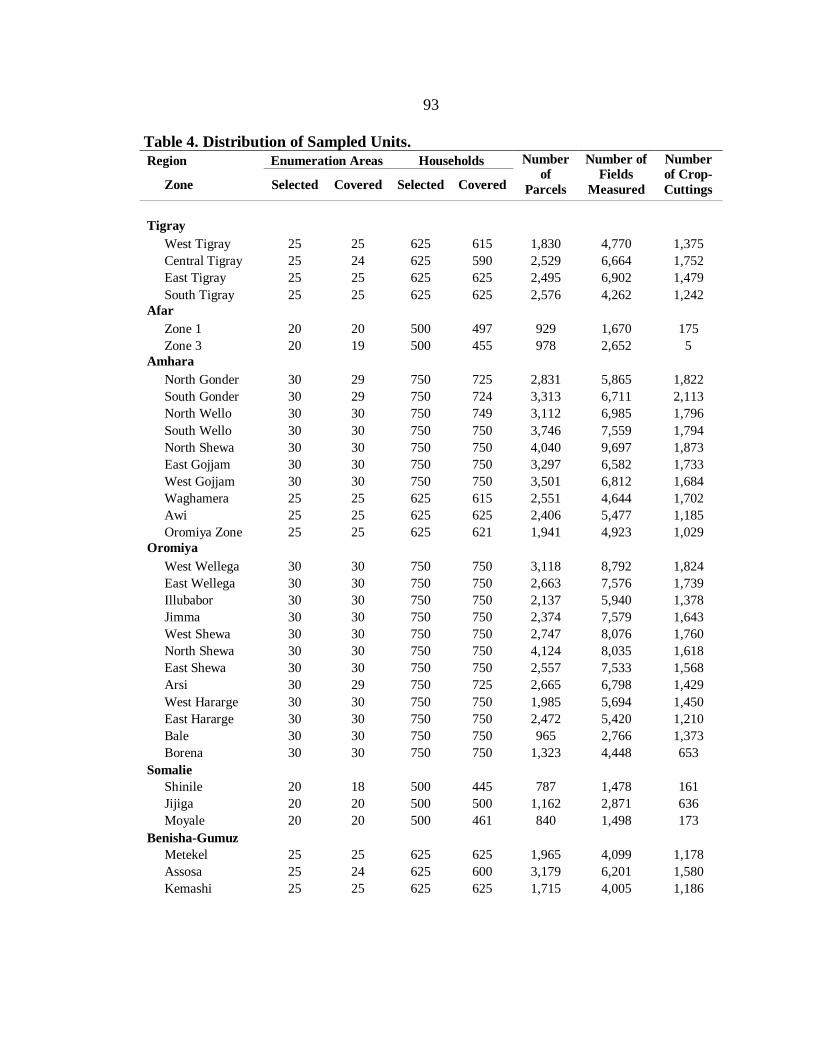
93
Table 4. Distribution of Sampled Units.
Region Enumeration Areas Households Number
of
Parcels
Number of
Fields
Measured
Number
of Crop-
Cuttings Zone Selected Covered Selected Covered
Tigray
West Tigray 25 25 625 615 1,830 4,770 1,375
Central Tigray 25 24 625 590 2,529 6,664 1,752
East Tigray 25 25 625 625 2,495 6,902 1,479
South Tigray 25 25 625 625 2,576 4,262 1,242
Afar
Zone 1 20 20 500 497 929 1,670 175
Zone 3 20 19 500 455 978 2,652 5
Amhara
North Gonder 30 29 750 725 2,831 5,865 1,822
South Gonder 30 29 750 724 3,313 6,711 2,113
North Wello 30 30 750 749 3,112 6,985 1,796
South Wello 30 30 750 750 3,746 7,559 1,794
North Shewa 30 30 750 750 4,040 9,697 1,873
East Gojjam 30 30 750 750 3,297 6,582 1,733
West Gojjam 30 30 750 750 3,501 6,812 1,684
Waghamera 25 25 625 615 2,551 4,644 1,702
Awi 25 25 625 625 2,406 5,477 1,185
Oromiya Zone 25 25 625 621 1,941 4,923 1,029
Oromiya
West Wellega 30 30 750 750 3,118 8,792 1,824
East Wellega 30 30 750 750 2,663 7,576 1,739
Illubabor 30 30 750 750 2,137 5,940 1,378
Jimma 30 30 750 750 2,374 7,579 1,643
West Shewa 30 30 750 750 2,747 8,076 1,760
North Shewa 30 30 750 750 4,124 8,035 1,618
East Shewa 30 30 750 750 2,557 7,533 1,568
Arsi 30 29 750 725 2,665 6,798 1,429
West Hararge 30 30 750 750 1,985 5,694 1,450
East Hararge 30 30 750 750 2,472 5,420 1,210
Bale 30 30 750 750 965 2,766 1,373
Borena 30 30 750 750 1,323 4,448 653
Somalie
Shinile 20 18 500 445 787 1,478 161
Jijiga 20 20 500 500 1,162 2,871 636
Moyale 20 20 500 461 840 1,498 173
Benisha-Gumuz
Metekel 25 25 625 625 1,965 4,099 1,178
Assosa 25 24 625 600 3,179 6,201 1,580
Kemashi 25 25 625 625 1,715 4,005 1,186
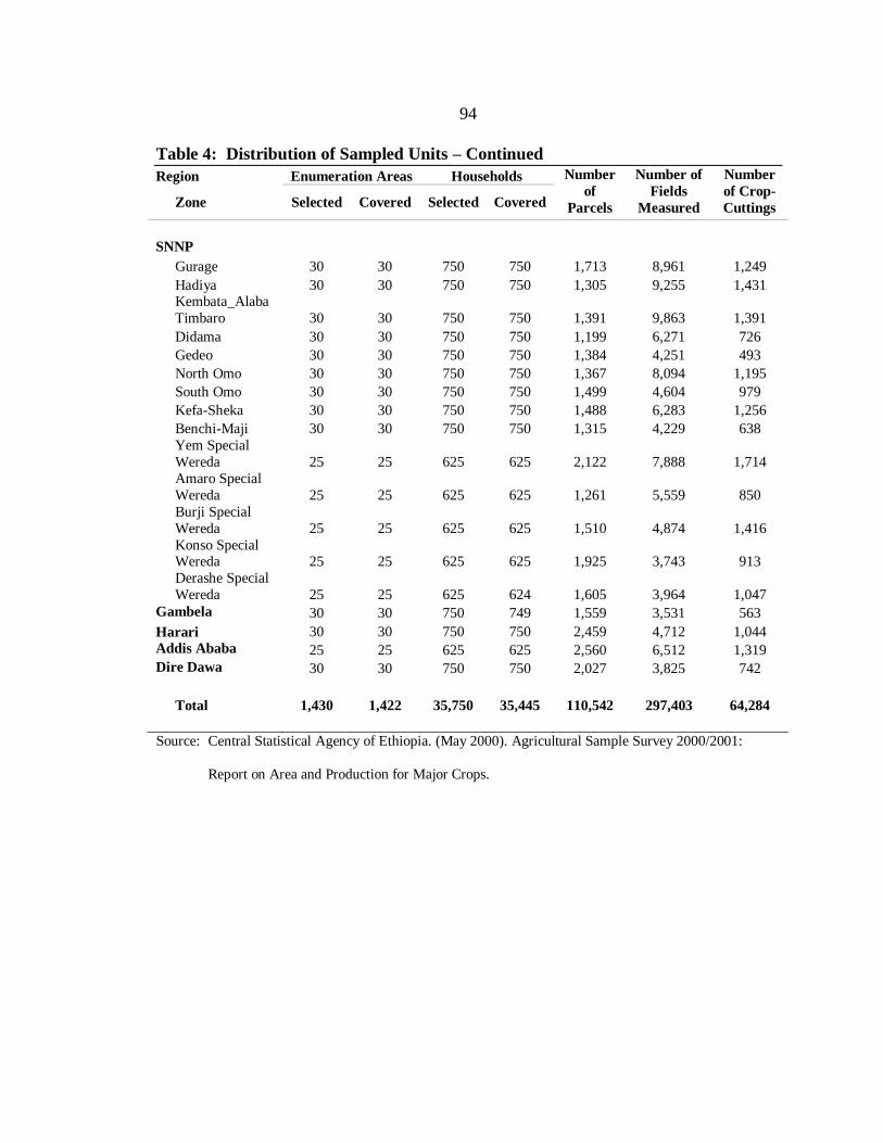
94
Table 4: Distribution of Sampled Units – Continued
Region Enumeration Areas Households Number
of
Parcels
Number of
Fields
Measured
Number
of Crop-
Cuttings Zone Selected Covered Selected Covered
SNNP
Gurage 30 30 750 750 1,713 8,961 1,249
Hadiya 30 30 750 750 1,305 9,255 1,431
Kembata_Alaba
Timbaro 30 30 750 750 1,391 9,863 1,391
Didama 30 30 750 750 1,199 6,271 726
Gedeo 30 30 750 750 1,384 4,251 493
North Omo 30 30 750 750 1,367 8,094 1,195
South Omo 30 30 750 750 1,499 4,604 979
Kefa-Sheka 30 30 750 750 1,488 6,283 1,256
Benchi-Maji 30 30 750 750 1,315 4,229 638
Yem Special
Wereda 25 25 625 625 2,122 7,888 1,714
Amaro Special
Wereda 25 25 625 625 1,261 5,559 850
Burji Special
Wereda 25 25 625 625 1,510 4,874 1,416
Konso Special Wereda 25 25 625 625 1,925 3,743 913
Derashe Special
Wereda 25 25 625 624 1,605 3,964 1,047
Gambela 30 30 750 749 1,559 3,531 563
Harari 30 30 750 750 2,459 4,712 1,044
Addis Ababa 25 25 625 625 2,560 6,512 1,319
Dire Dawa 30 30 750 750 2,027 3,825 742
Total 1,430 1,422 35,750 35,445 110,542 297,403 64,284
Source: Central Statistical Agency of Ethiopia. (May 2000). Agricultural Sample Survey 2000/2001:
Report on Area and Production for Major Crops.
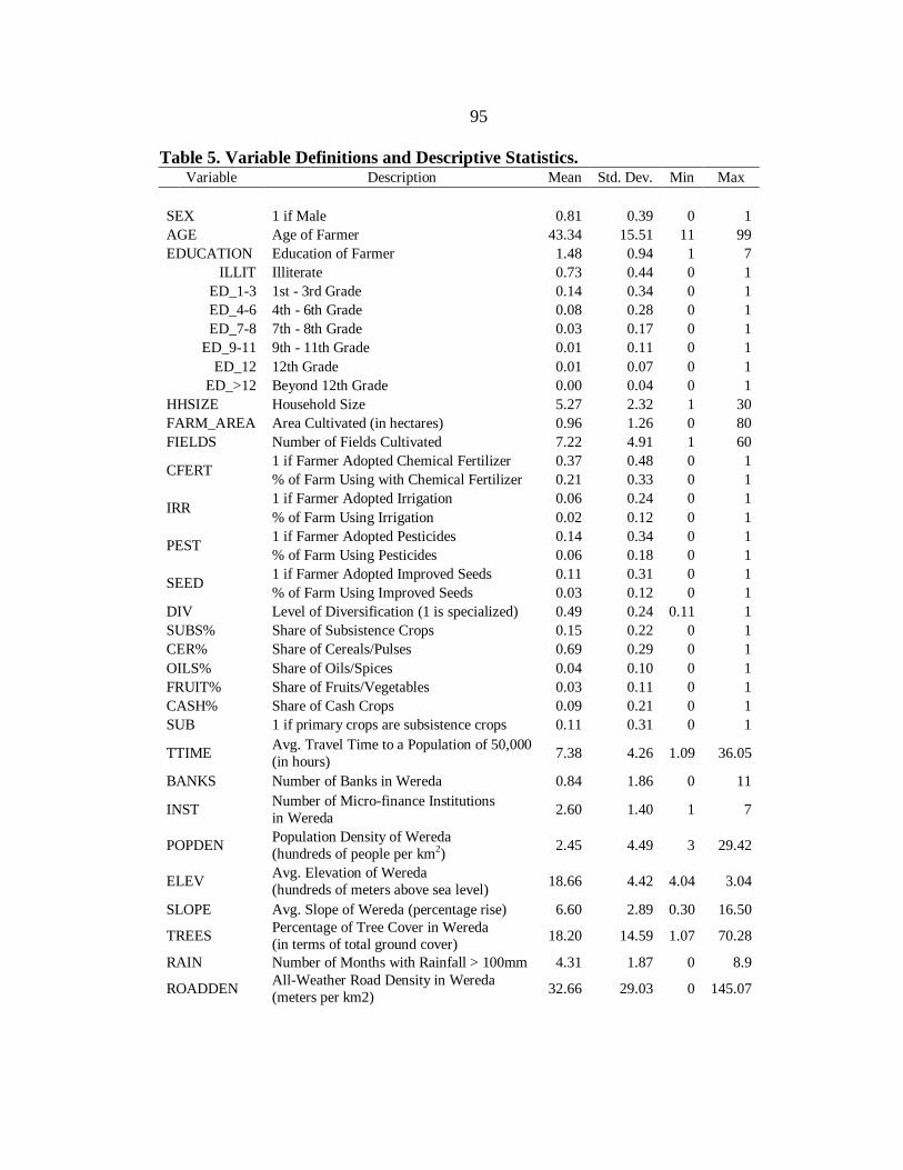
95
Table 5. Variable Definitions and Descriptive Statistics. Variable Description Mean Std. Dev. Min Max
SEX 1 if Male 0.81 0.39 0 1
AGE Age of Farmer 43.34 15.51 11 99
EDUCATION Education of Farmer 1.48 0.94 1 7
ILLIT Illiterate 0.73 0.44 0 1
ED_1-3 1st - 3rd Grade 0.14 0.34 0 1
ED_4-6 4th - 6th Grade 0.08 0.28 0 1
ED_7-8 7th - 8th Grade 0.03 0.17 0 1
ED_9-11 9th - 11th Grade 0.01 0.11 0 1
ED_12 12th Grade 0.01 0.07 0 1
ED_>12 Beyond 12th Grade 0.00 0.04 0 1
HHSIZE Household Size 5.27 2.32 1 30
FARM_AREA Area Cultivated (in hectares) 0.96 1.26 0 80
FIELDS Number of Fields Cultivated 7.22 4.91 1 60
CFERT 1 if Farmer Adopted Chemical Fertilizer 0.37 0.48 0 1
% of Farm Using with Chemical Fertilizer 0.21 0.33 0 1
IRR 1 if Farmer Adopted Irrigation 0.06 0.24 0 1
% of Farm Using Irrigation 0.02 0.12 0 1
PEST 1 if Farmer Adopted Pesticides 0.14 0.34 0 1
% of Farm Using Pesticides 0.06 0.18 0 1
SEED 1 if Farmer Adopted Improved Seeds 0.11 0.31 0 1
% of Farm Using Improved Seeds 0.03 0.12 0 1
DIV Level of Diversification (1 is specialized) 0.49 0.24 0.11 1
SUBS% Share of Subsistence Crops 0.15 0.22 0 1
CER% Share of Cereals/Pulses 0.69 0.29 0 1
OILS% Share of Oils/Spices 0.04 0.10 0 1
FRUIT% Share of Fruits/Vegetables 0.03 0.11 0 1
CASH% Share of Cash Crops 0.09 0.21 0 1
SUB 1 if primary crops are subsistence crops 0.11 0.31 0 1
TTIME Avg. Travel Time to a Population of 50,000
(in hours) 7.38 4.26 1.09 36.05
BANKS Number of Banks in Wereda 0.84 1.86 0 11
INST Number of Micro-finance Institutions
in Wereda 2.60 1.40 1 7
POPDEN Population Density of Wereda
(hundreds of people per km2) 2.45 4.49 3 29.42
ELEV Avg. Elevation of Wereda
(hundreds of meters above sea level) 18.66 4.42 4.04 3.04
SLOPE Avg. Slope of Wereda (percentage rise) 6.60 2.89 0.30 16.50
TREES Percentage of Tree Cover in Wereda
(in terms of total ground cover) 18.20 14.59 1.07 70.28
RAIN Number of Months with Rainfall > 100mm 4.31 1.87 0 8.9
ROADDEN All-Weather Road Density in Wereda
(meters per km2) 32.66 29.03 0 145.07
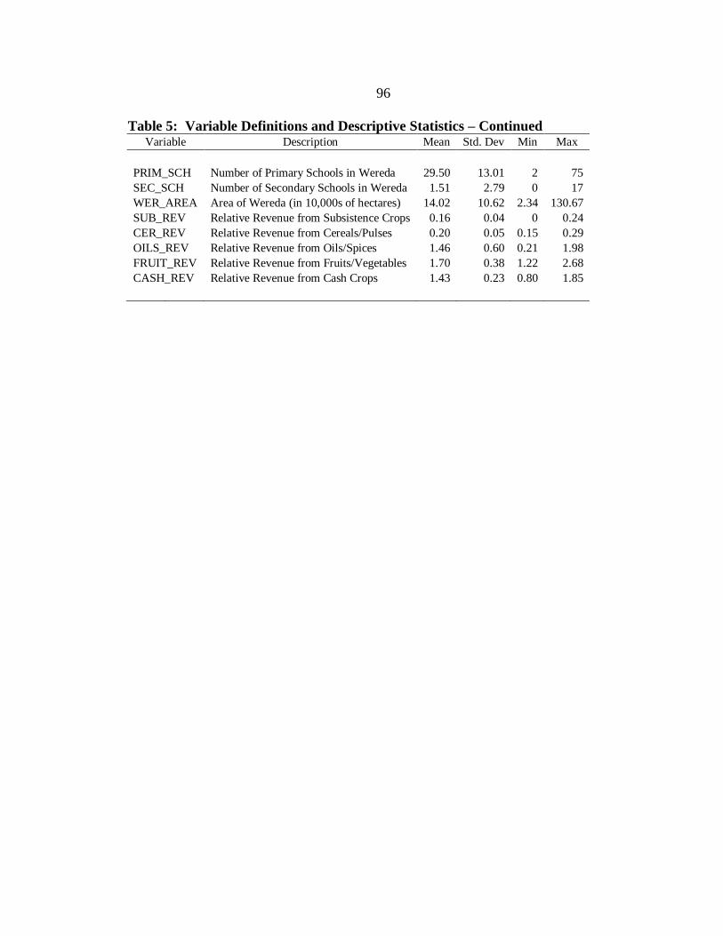
96
Table 5: Variable Definitions and Descriptive Statistics – Continued Variable Description Mean Std. Dev Min Max
PRIM_SCH Number of Primary Schools in Wereda 29.50 13.01 2 75
SEC_SCH Number of Secondary Schools in Wereda 1.51 2.79 0 17
WER_AREA Area of Wereda (in 10,000s of hectares) 14.02 10.62 2.34 130.67
SUB_REV Relative Revenue from Subsistence Crops 0.16 0.04 0 0.24
CER_REV Relative Revenue from Cereals/Pulses 0.20 0.05 0.15 0.29
OILS_REV Relative Revenue from Oils/Spices 1.46 0.60 0.21 1.98
FRUIT_REV Relative Revenue from Fruits/Vegetables 1.70 0.38 1.22 2.68
CASH_REV Relative Revenue from Cash Crops 1.43 0.23 0.80 1.85
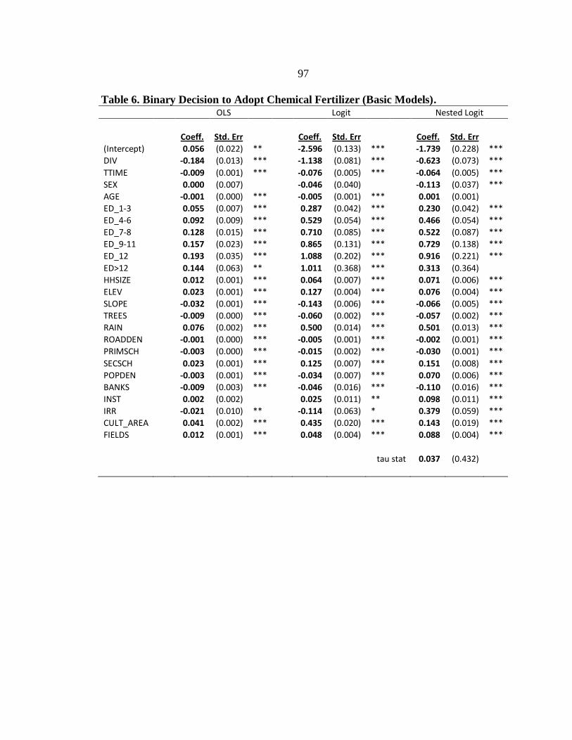
97
Table 6. Binary Decision to Adopt Chemical Fertilizer (Basic Models).
OLS
Logit
Nested Logit
Coeff. Std. Err
Coeff. Std. Err
Coeff. Std. Err
(Intercept)
0.056 (0.022) **
-2.596 (0.133) ***
-1.739 (0.228) ***
DIV
-0.184 (0.013) ***
-1.138 (0.081) ***
-0.623 (0.073) ***
TTIME
-0.009 (0.001) ***
-0.076 (0.005) ***
-0.064 (0.005) ***
SEX
0.000 (0.007)
-0.046 (0.040)
-0.113 (0.037) ***
AGE
-0.001 (0.000) ***
-0.005 (0.001) ***
0.001 (0.001) ED_1-3
0.055 (0.007) ***
0.287 (0.042) ***
0.230 (0.042) ***
ED_4-6
0.092 (0.009) ***
0.529 (0.054) ***
0.466 (0.054) ***
ED_7-8
0.128 (0.015) ***
0.710 (0.085) ***
0.522 (0.087) ***
ED_9-11
0.157 (0.023) ***
0.865 (0.131) ***
0.729 (0.138) ***
ED_12
0.193 (0.035) ***
1.088 (0.202) ***
0.916 (0.221) ***
ED>12
0.144 (0.063) **
1.011 (0.368) ***
0.313 (0.364) HHSIZE
0.012 (0.001) ***
0.064 (0.007) ***
0.071 (0.006) ***
ELEV
0.023 (0.001) ***
0.127 (0.004) ***
0.076 (0.004) ***
SLOPE
-0.032 (0.001) ***
-0.143 (0.006) ***
-0.066 (0.005) ***
TREES
-0.009 (0.000) ***
-0.060 (0.002) ***
-0.057 (0.002) ***
RAIN
0.076 (0.002) ***
0.500 (0.014) ***
0.501 (0.013) ***
ROADDEN
-0.001 (0.000) ***
-0.005 (0.001) ***
-0.002 (0.001) ***
PRIMSCH
-0.003 (0.000) ***
-0.015 (0.002) ***
-0.030 (0.001) ***
SECSCH
0.023 (0.001) ***
0.125 (0.007) ***
0.151 (0.008) ***
POPDEN
-0.003 (0.001) ***
-0.034 (0.007) ***
0.070 (0.006) ***
BANKS
-0.009 (0.003) ***
-0.046 (0.016) ***
-0.110 (0.016) ***
INST
0.002 (0.002)
0.025 (0.011) **
0.098 (0.011) ***
IRR
-0.021 (0.010) **
-0.114 (0.063) *
0.379 (0.059) ***
CULT_AREA
0.041 (0.002) ***
0.435 (0.020) ***
0.143 (0.019) ***
FIELDS
0.012 (0.001) ***
0.048 (0.004) ***
0.088 (0.004) ***
tau stat 0.037 (0.432)
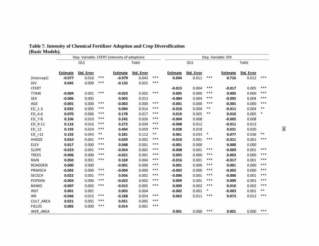
98
Table 7. Intensity of Chemical Fertilizer Adoption and Crop Diversification
(Basic Models).
Dep. Variable: CFERT (intensity of adoption)
Dep. Variable: DIV
OLS
Tobit
OLS
Tobit
Estimate Std. Error
Estimate Std. Error
Estimate Std. Error
Estimate Std. Error
(Intercept)
-0.077 0.016 ***
-0.979 0.043 ***
0.694 0.011 ***
0.716 0.012 ***
DIV
0.045 0.009 ***
-0.135 0.025 *** CFERT
-0.013 0.004 ***
-0.017 0.005 ***
TTIME
-0.004 0.001 ***
-0.023 0.002 ***
0.005 0.000 ***
0.005 0.000 ***
SEX
-0.006 0.005
0.003 0.013
-0.084 0.004 ***
-0.092 0.004 ***
AGE
-0.001 0.000 ***
-0.002 0.000 ***
-0.001 0.000 ***
-0.001 0.000 ***
ED_1-3
0.035 0.005 ***
0.094 0.014 ***
-0.010 0.004 **
-0.011 0.004 **
ED_4-6
0.070 0.006 ***
0.178 0.017 ***
0.010 0.005 **
0.010 0.005 *
ED_7-8
0.106 0.010 ***
0.242 0.026 ***
-0.004 0.008
-0.005 0.008 ED_9-11
0.116 0.016 ***
0.272 0.039 ***
-0.008 0.012
-0.011 0.013
ED_12
0.193 0.024 ***
0.404 0.059 ***
0.028 0.018
0.031 0.020 ED_>12
0.102 0.043 **
0.281 0.112 **
0.061 0.033 *
0.077 0.036 **
HHSIZE
0.010 0.001 ***
0.029 0.002 ***
-0.010 0.001 ***
-0.011 0.001 ***
ELEV
0.017 0.000 ***
0.048 0.001 ***
-0.001 0.000
0.000 0.000 SLOPE
-0.023 0.001 ***
-0.054 0.002 ***
-0.008 0.001 ***
-0.009 0.001 ***
TREES
-0.006 0.000 ***
-0.021 0.001 ***
0.003 0.000 ***
0.003 0.000 ***
RAIN
0.050 0.001 ***
0.169 0.004 ***
-0.016 0.001 ***
-0.017 0.001 ***
ROADDEN
0.000 0.000
-0.001 0.000 ***
0.001 0.000 ***
0.001 0.000 ***
PRIMSCH
-0.002 0.000 ***
-0.004 0.000 ***
-0.002 0.000 ***
-0.002 0.000 ***
SECSCH
0.022 0.001 ***
0.056 0.002 ***
-0.006 0.001 ***
-0.006 0.001 ***
POPDEN
-0.003 0.000 ***
-0.022 0.002 ***
0.009 0.001 ***
0.009 0.001 ***
BANKS
-0.007 0.002 ***
-0.015 0.005 ***
0.009 0.002 ***
0.010 0.002 ***
INST
0.001 0.001
0.003 0.004
-0.002 0.001 *
-0.003 0.001 **
IRR
-0.046 0.015 ***
-0.268 0.054 ***
0.063 0.011 ***
0.073 0.012 ***
CULT_AREA
0.021 0.001 ***
0.051 0.005 *** FIELDS
0.005 0.000 ***
0.014 0.001 ***
WER_AREA
0.001 0.000 ***
0.001 0.000 ***
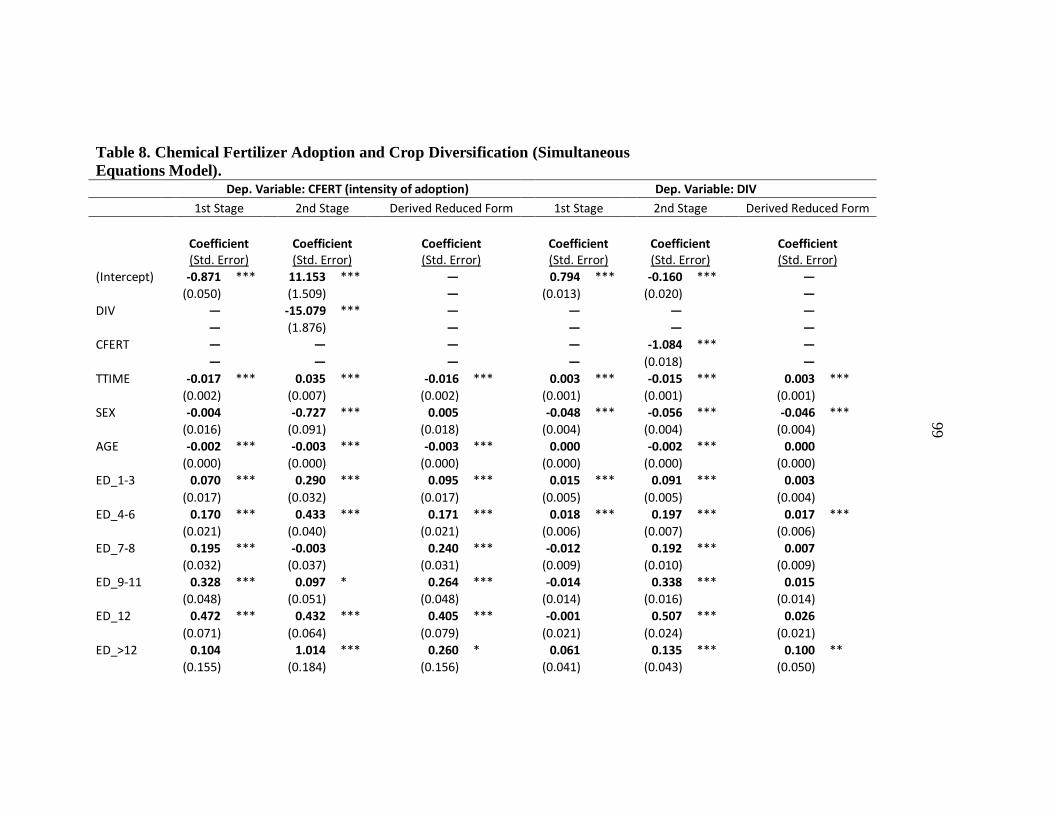
Table 8. Chemical Fertilizer Adoption and Crop Diversification (Simultaneous
Equations Model).
Dep. Variable: CFERT (intensity of adoption)
Dep. Variable: DIV
1st Stage
2nd Stage
Derived Reduced Form
1st Stage
2nd Stage
Derived Reduced Form
Coefficient (Std. Error)
Coefficient (Std. Error)
Coefficient (Std. Error)
Coefficient (Std. Error)
Coefficient (Std. Error)
Coefficient (Std. Error)
(Intercept)
-0.871 ***
11.153 ***
―
0.794 ***
-0.160 ***
―
(0.050)
(1.509)
―
(0.013)
(0.020)
―
DIV
―
-15.079 ***
―
―
―
―
―
(1.876)
―
―
―
―
CFERT
―
―
―
―
-1.084 ***
―
―
―
―
―
(0.018)
―
TTIME
-0.017 ***
0.035 ***
-0.016 ***
0.003 ***
-0.015 ***
0.003 ***
(0.002)
(0.007)
(0.002)
(0.001)
(0.001)
(0.001)
SEX
-0.004
-0.727 ***
0.005
-0.048 ***
-0.056 ***
-0.046 ***
(0.016)
(0.091)
(0.018)
(0.004)
(0.004)
(0.004)
AGE
-0.002 ***
-0.003 ***
-0.003 ***
0.000
-0.002 ***
0.000
(0.000)
(0.000)
(0.000)
(0.000)
(0.000)
(0.000)
ED_1-3
0.070 ***
0.290 ***
0.095 ***
0.015 ***
0.091 ***
0.003
(0.017)
(0.032)
(0.017)
(0.005)
(0.005)
(0.004)
ED_4-6
0.170 ***
0.433 ***
0.171 ***
0.018 ***
0.197 ***
0.017 ***
(0.021)
(0.040)
(0.021)
(0.006)
(0.007)
(0.006)
ED_7-8
0.195 ***
-0.003
0.240 ***
-0.012
0.192 ***
0.007
(0.032)
(0.037)
(0.031)
(0.009)
(0.010)
(0.009)
ED_9-11
0.328 ***
0.097 *
0.264 ***
-0.014
0.338 ***
0.015
(0.048)
(0.051)
(0.048)
(0.014)
(0.016)
(0.014)
ED_12
0.472 ***
0.432 ***
0.405 ***
-0.001
0.507 ***
0.026
(0.071)
(0.064)
(0.079)
(0.021)
(0.024)
(0.021)
ED_>12
0.104
1.014 ***
0.260 *
0.061
0.135 ***
0.100 **
(0.155)
(0.184)
(0.156)
(0.041)
(0.043)
(0.050)
99

Table 8: Chemical Fertilizer Adoption and Crop Diversification (Simultaneous Equations Model) - Continued
Dep. Variable: CFERT (intensity of adoption)
Dep. Variable: DIV
1st Stage
2nd Stage
Derived Reduced Form
1st Stage
2nd Stage
Derived Reduced Form
Coefficient (Std. Error)
Coefficient (Std. Error)
Coefficient (Std. Error)
Coefficient (Std. Error)
Coefficient (Std. Error)
Coefficient (Std. Error)
HHSIZE
0.030 ***
0.062 ***
0.029 ***
0.002 ***
0.034 ***
0.001 **
(0.003)
(0.005)
(0.003)
(0.001)
(0.001)
(0.001)
ELEV
0.042 ***
-0.001
0.045 ***
-0.003 ***
0.044 ***
-0.002 ***
(0.002
(0.006)
(0.002)
(0.000)
(0.001)
(0.000)
SLOPE
-0.058 ***
-0.135 ***
-0.061 ***
-0.005 ***
-0.070 ***
-0.004 ***
(0.002)
(0.011)
(0.002)
(0.001)
(0.001)
(0.001)
TREES
-0.022 ***
-0.005 ***
-0.021 ***
0.001 ***
-0.022 ***
0.001 ***
(0.001)
(0.002)
(0.001)
(0.000)
(0.000)
(0.000)
RAIN
0.164 ***
0.049 ***
0.155 ***
-0.007 ***
0.166 ***
-0.008 ***
(0.005)
(0.015)
(0.005)
(0.001)
(0.003)
(0.001)
ROADDEN
-0.002 ***
0.009 ***
-0.002 ***
0.001 ***
-0.001 ***
0.001 ***
(0.000)
(0.001)
(0.000)
(0.000)
(0.000)
(0.000)
PRIMSCH
-0.003 ***
-0.023 ***
-0.003 ***
-0.001 ***
-0.005 ***
-0.001 ***
(0.001)
(0.002)
(0.001)
(0.000)
(0.000)
(0.000)
SECSCH
0.054 ***
0.011 **
0.053 ***
-0.003 ***
0.054 ***
-0.003 ***
(0.003)
(0.006)
(0.003)
(0.001)
(0.001)
(0.001)
POPDEN
-0.029 ***
0.105 ***
-0.030 ***
0.009 ***
-0.025 ***
0.009 ***
(0.003)
(0.016)
(0.003)
(0.001)
(0.001)
(0.001)
BANKS
-0.015 **
0.023 ***
-0.013 **
0.003
-0.009 ***
0.004 **
(0.006)
(0.007)
(0.007)
(0.002)
(0.002)
(0.002)
INST
0.017 ***
-0.023 ***
0.014 ***
-0.003 **
0.014 ***
-0.002 *
(0.005)
(0.005)
(0.005)
(0.001)
(0.001)
(0.001)
100

Table 8: Chemical Fertilizer Adoption and Crop Diversification (Simultaneous Equations Model) - Continued
Dep. Variable: CFERT (intensity of adoption)
Dep. Variable: DIV
1st Stage
2nd Stage
Derived Reduced Form
1st Stage
2nd Stage
Derived Reduced Form
Coefficient (Std. Error)
Coefficient (Std. Error)
Coefficient (Std. Error)
Coefficient (Std. Error)
Coefficient (Std. Error)
Coefficient (Std. Error)
IRR
-0.004
0.099 ***
-0.077 ***
0.007
-0.010
0.005
(0.025)
(0.026)
(0.026)
(0.006)
(0.007)
(0.006)
CULT_AREA
0.044 ***
-0.019 **
0.005
-0.004 ***
―
-0.004
(0.006)
(0.008)
(0.005)
(0.001)
―
(0.004)
FIELDS
0.015 ***
-0.394 ***
0.029 ***
-0.027 ***
―
-0.028 ***
(0.001)
(0.051)
(0.003)
(0.000)
―
(0.001)
WER_AREA
-0.007 ***
―
-0.008 ***
0.000 **
-0.007 ***
0.001 **
(0.001)
―
(0.001)
(0.000)
(0.000)
(0.000)
101
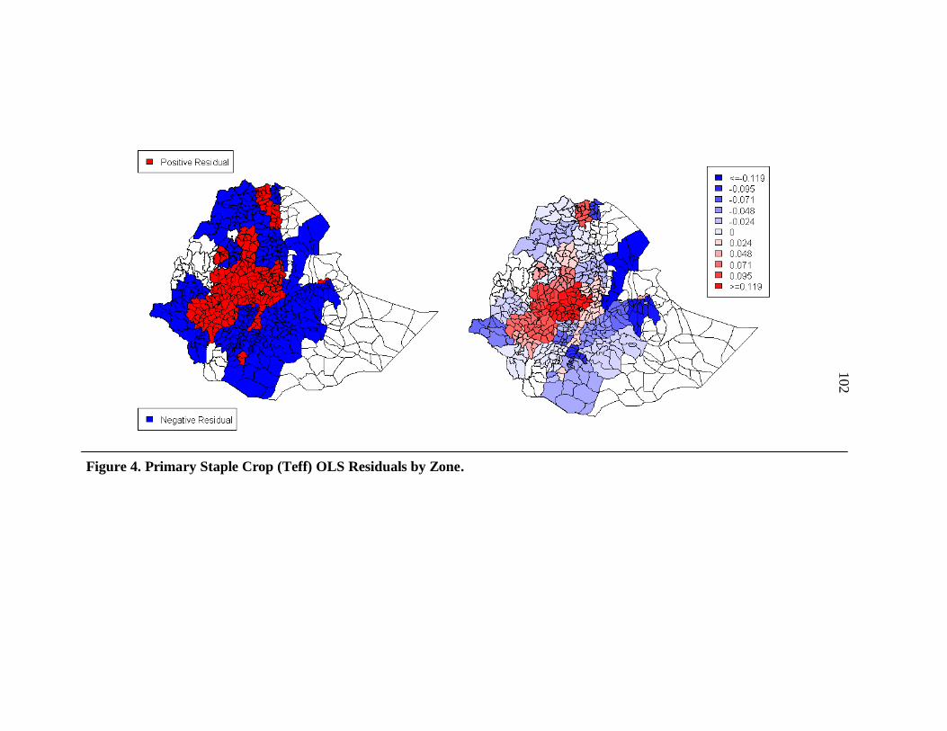
Figure 4. Primary Staple Crop (Teff) OLS Residuals by Zone.
102

Figure 5. Cereal and Pulse Crop OLS Residuals by Zone.
103
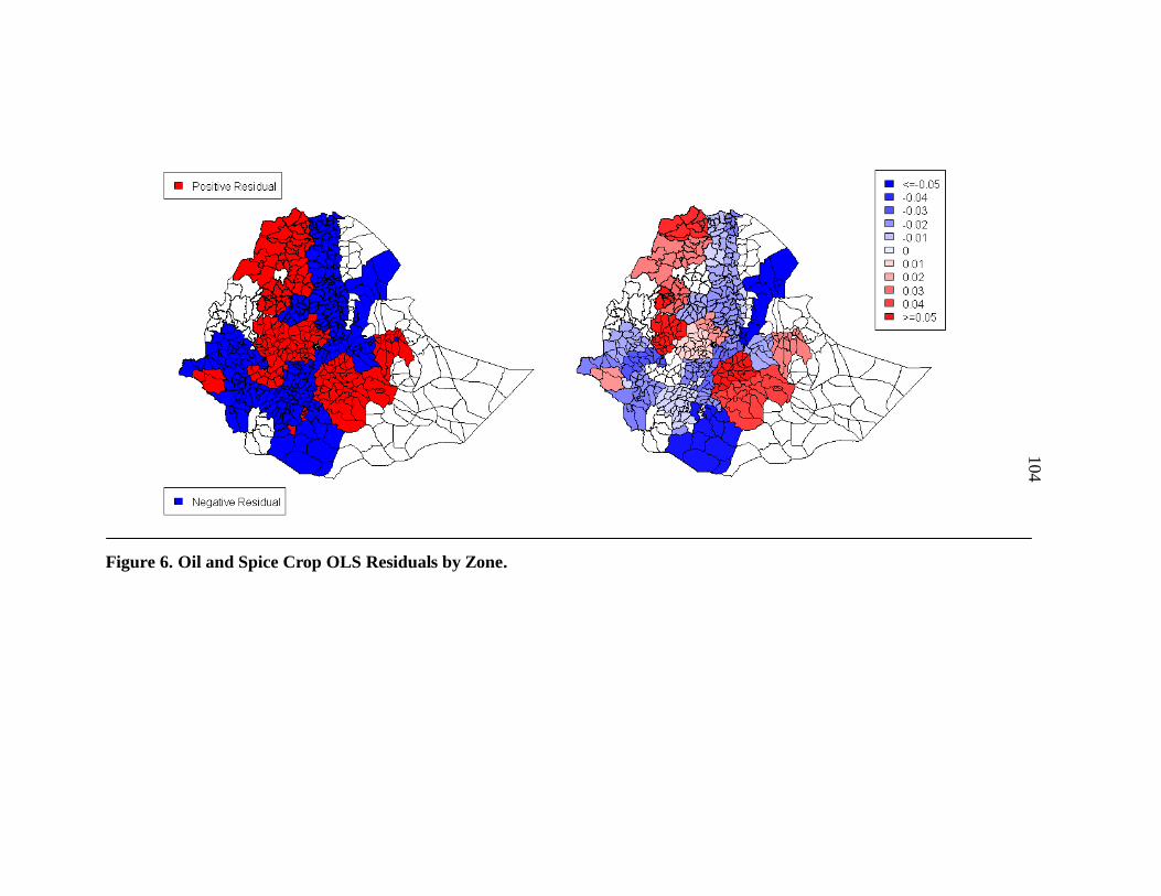
Figure 6. Oil and Spice Crop OLS Residuals by Zone.
104
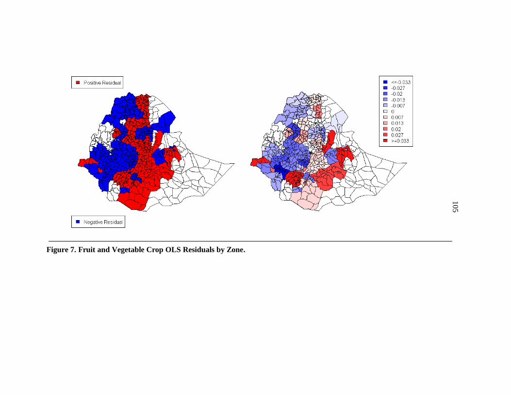
Figure 7. Fruit and Vegetable Crop OLS Residuals by Zone.
105
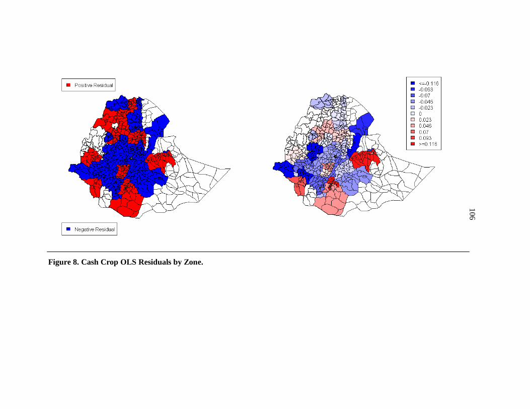
Figure 8. Cash Crop OLS Residuals by Zone.
106

Table 9. Crop Share Regressions using an OLS Model.
Primary Staple Crop
Cereals/Pulses
Oils/Spices
Fruits/Vegetables
Cash Crops
Coeff. Std. Err
Coeff. Std. Err
Coeff. Std. Err
Coeff. Std. Err
Coeff. Std. Err
(Intercept) -0.023 (0.014)
0.937 (0.018) ***
-0.044 (0.007) ***
0.062 (0.007) ***
0.067 (0.012) ***
TTIME -0.004 (0.000) *** 0.009 (0.001) ***
-0.001 (0.000) ***
0.001 (0.000) ***
-0.005 (0.000) ***
CER_REV 0.400 (0.040) *** -0.554 (0.050) ***
0.275 (0.018) ***
0.034 (0.020) *
-0.154 (0.033) ***
FRUIT_REV 0.022 (0.005) *** -0.026 (0.007) ***
0.013 (0.002) ***
-0.016 (0.003) ***
0.006 (0.004) SEX 0.033 (0.004) *** -0.018 (0.004) ***
0.006 (0.002) ***
-0.007 (0.002) ***
-0.014 (0.003) ***
AGE -0.001 (0.000) *** 0.000 (0.000)
0.000 (0.000) *
0.000 (0.000) *
0.000 (0.000) ***
ED_1-3 -0.007 (0.004) * -0.013 (0.005) **
0.003 (0.002)
0.002 (0.002)
0.015 (0.003) ***
ED_4-6 -0.006 (0.005)
-0.027 (0.006) ***
-0.003 (0.002)
0.008 (0.002) ***
0.028 (0.004) ***
ED_7-8 0.005 (0.008)
-0.056 (0.010) ***
-0.001 (0.004)
0.017 (0.004) ***
0.036 (0.006) ***
ED_9-11 0.006 (0.012)
-0.057 (0.015) ***
0.005 (0.005)
0.024 (0.006) ***
0.023 (0.010) **
ED_12 -0.016 (0.018)
-0.029 (0.023)
-0.013 (0.008)
0.031 (0.009) ***
0.028 (0.015) *
ED_>12 -0.044 (0.032)
-0.087 (0.041) **
0.011 (0.015)
0.082 (0.016) ***
0.039 (0.027) FIELDS 0.003 (0.000) *** -0.004 (0.000) ***
0.001 (0.000) ***
-0.001 (0.000) ***
0.002 (0.000) ***
IRR 0.006 (0.005)
-0.095 (0.007) ***
-0.003 (0.003)
0.034 (0.003) ***
0.058 (0.005) ***
HHSIZE 0.001 (0.001) ** 0.001 (0.001) *
0.000 (0.000)
-0.001 (0.000) ***
-0.002 (0.000) ***
AREA 0.000 (0.000)
-0.003 (0.000) ***
0.001 (0.000) ***
0.000 (0.000)
0.002 (0.000) ***
BANKS 0.004 (0.002) ** -0.014 (0.002) ***
0.000 (0.001)
-0.002 (0.001) ***
0.012 (0.001) ***
INST 0.001 (0.001)
0.008 (0.001) ***
-0.002 (0.001) ***
-0.003 (0.001) ***
-0.004 (0.001) ***
POPDEN -0.008 (0.001) *** 0.005 (0.001) ***
-0.003 (0.000) ***
0.001 (0.000) ***
0.004 (0.000) ***
ELEV 0.003 (0.000) *** -0.001 (0.000) ***
0.001 (0.000) ***
-0.001 (0.000) ***
-0.002 (0.000) ***
SLOPE 0.001 (0.001) *** 0.001 (0.001) **
-0.004 (0.000) ***
-0.002 (0.000) ***
0.003 (0.000) ***
TREES -0.001 (0.000) *** -0.004 (0.000) ***
0.000 (0.000)
-0.001 (0.000) ***
0.006 (0.000) ***
RAIN 0.013 (0.001) *** -0.016 (0.001) ***
0.006 (0.001) ***
0.007 (0.001) ***
-0.009 (0.001) ***
ROADDEN 0.000 (0.000) *** -0.001 (0.000) ***
0.000 (0.000) ***
0.000 (0.000) ***
0.001 (0.000) ***
PRIM_SCHL 0.000 (0.000) * 0.003 (0.000) ***
0.000 (0.000) ***
0.000 (0.000)
-0.003 (0.000) ***
SEC_SCHL -0.008 (0.001) *** -0.003 (0.001) ***
0.005 (0.000) ***
0.001 (0.000)
0.006 (0.001) ***
107
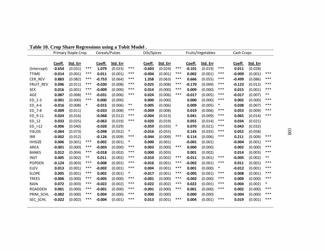
Table 10. Crop Share Regressions using a Tobit Model .
Primary Staple Crop Cereals/Pulses
Oils/Spices Fruits/Vegetables
Cash Crops
Coeff. Std. Err
Coeff. Std. Err
Coeff. Std. Err
Coeff. Std. Err
Coeff. Std. Err
(Intercept) -0.654 (0.031) *** 1.079 (0.023) ***
-0.603 (0.024) *** -0.101 (0.019) ***
0.011 (0.028) TTIME -0.014 (0.001) *** 0.011 (0.001) ***
-0.004 (0.001) *** 0.002 (0.001) ***
-0.009 (0.001) ***
CER_REV 0.883 (0.082) *** -0.753 (0.064) ***
1.358 (0.063) *** 0.666 (0.055) ***
-0.499 (0.086) ***
FRUIT_REV 0.096 (0.011) *** -0.030 (0.008) ***
0.025 (0.008) *** -0.170 (0.009) ***
-0.123 (0.012) ***
SEX 0.016 (0.001) *** -0.009 (0.000) ***
0.014 (0.000) *** 0.009 (0.000) ***
0.015 (0.001) ***
AGE 0.087 (0.008) *** -0.031 (0.006) ***
0.024 (0.006) *** -0.017 (0.005) ***
-0.017 (0.007) **
ED_1-3 -0.001 (0.000) *** 0.000 (0.000)
0.000 (0.000)
0.000 (0.000) ***
0.002 (0.000) ***
ED_4-6 -0.016 (0.008) * -0.015 (0.006) **
0.005 (0.006)
0.009 (0.005) *
0.038 (0.007) ***
ED_7-8 -0.009 (0.011)
-0.033 (0.008) ***
-0.009 (0.008)
0.019 (0.006) ***
0.053 (0.009) ***
ED_9-11 0.024 (0.016)
-0.068 (0.012) ***
-0.004 (0.013)
0.041 (0.009) ***
0.065 (0.014) ***
ED_12 0.033 (0.025)
-0.063 (0.019) ***
0.020 (0.019)
0.055 (0.014) ***
0.034 (0.021) ED_>12 -0.006 (0.040)
-0.028 (0.029)
-0.059 (0.033) * 0.070 (0.021) ***
0.043 (0.032)
FIELDS -0.064 (0.073)
-0.098 (0.052) *
-0.016 (0.055)
0.145 (0.035) ***
0.052 (0.058) IRR -0.002 (0.012)
-0.126 (0.009) ***
-0.044 (0.009) *** 0.114 (0.006) ***
0.211 (0.009) ***
HHSIZE 0.006 (0.001) *** 0.002 (0.001) *
0.000 (0.001)
-0.001 (0.001)
-0.004 (0.001) ***
AREA -0.001 (0.000) *** -0.003 (0.000) ***
0.003 (0.000) *** 0.000 (0.000)
0.002 (0.000) ***
BANKS 0.012 (0.004) *** -0.018 (0.002) ***
0.000 (0.003)
0.001 (0.002)
0.014 (0.003) ***
INST 0.005 (0.002) ** 0.011 (0.002) ***
-0.010 (0.002) *** -0.011 (0.001) ***
-0.005 (0.002) **
POPDEN -0.124 (0.003) *** 0.008 (0.001) ***
-0.016 (0.001) *** -0.002 (0.001) ***
0.011 (0.001) ***
ELEV 0.013 (0.001) *** -0.002 (0.001) ***
0.004 (0.001) *** 0.001 (0.000) *
-0.012 (0.001) ***
SLOPE 0.005 (0.001) *** 0.002 (0.001) *
-0.017 (0.001) *** -0.005 (0.001) ***
0.008 (0.001) ***
TREES -0.006 (0.000) *** -0.005 (0.000) ***
-0.001 (0.000) *** -0.002 (0.000) ***
0.009 (0.000) ***
RAIN 0.072 (0.003) *** -0.022 (0.002) ***
0.022 (0.002) *** 0.022 (0.001) ***
0.004 (0.002) *
ROADDEN 0.001 (0.000) *** -0.001 (0.000) ***
-0.001 (0.000) *** 0.001 (0.000) ***
0.002 (0.000) ***
PRIM_SCHL -0.002 (0.000) *** 0.004 (0.000) ***
0.000 (0.000)
0.000 (0.000)
-0.004 (0.000) ***
SEC_SCHL -0.022 (0.002) *** -0.004 (0.001) ***
0.013 (0.001) *** 0.004 (0.001) ***
0.019 (0.001) ***
108
109
APPENDIX B
SIMULTANEOUS EQUATION SIMULATION

110
Simultaneous Discrete Choice Model:
A Simulation
Following Train (2009), when faced with a decision, each household is assumed
to choose alternative j if the utility, Uj, from that alternative exceeds the utility, Ui, from
the set of alternatives i:
(A.1) .
The researcher does not observe the economic agent‘s utility, only their final decision, yj,
which is presented below and depends on parameters unknown to the researcher. The
unobserved, or latent, utility is modeled as,
(A.2) ,
where Rj is affected by a set of observable factors and εj is unobservable.
Assuming that latent utility can be modeled linearly as,
(A.3) ,
two types of choice sets may be observed:
(A.4)
Given the observable choice sets, the researcher is concerned with how well their
empirical representation approximates the underlying utility.
This section‘s simulations compare known values of utility to estimates from a
regression model, specifically, a simultaneous equation model using two limited
Discrete Censored
,
,
,
.
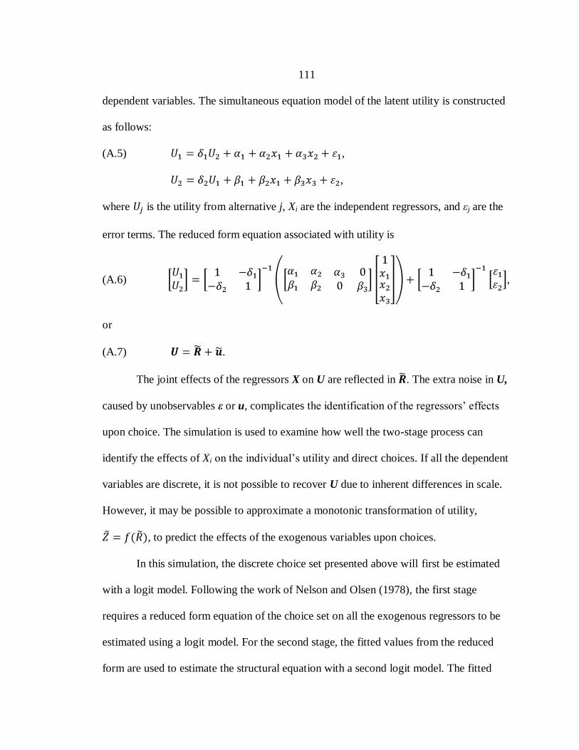
111
dependent variables. The simultaneous equation model of the latent utility is constructed
as follows:
(A.5) ,
,
where is the utility from alternative j, Xi are the independent regressors, and εj are the
error terms. The reduced form equation associated with utility is
(A.6) ,
or
(A.7) .
The joint effects of the regressors X on U are reflected in . The extra noise in U,
caused by unobservables ε or u, complicates the identification of the regressors‘ effects
upon choice. The simulation is used to examine how well the two-stage process can
identify the effects of Xi on the individual‘s utility and direct choices. If all the dependent
variables are discrete, it is not possible to recover U due to inherent differences in scale.
However, it may be possible to approximate a monotonic transformation of utility,
, to predict the effects of the exogenous variables upon choices.
In this simulation, the discrete choice set presented above will first be estimated
with a logit model. Following the work of Nelson and Olsen (1978), the first stage
requires a reduced form equation of the choice set on all the exogenous regressors to be
estimated using a logit model. For the second stage, the fitted values from the reduced
form are used to estimate the structural equation with a second logit model. The fitted

112
values from both stages are functions of the mean component of the reduced form utility
from equation (A.7), .
Figure 9 below plots the fitted values from the regression ( ) against the true
experimental utility values ( ). The top two plots are from the first-stage regression for
choices 1 and 2, and the bottom two plots are from the second-stage regression for the
same choices. The fitted values from the logit model very closely map to a monotonic
transformation of the underlying utility, . Although there is more noise in the second-
stage of the simultaneous equation model, the logit regression does an excellent job of
recovering a transformation of the mean component of utility. In fact, using a sample of
10,000 observations, the logit model was 98% accurate in predicting what the discrete
choices would have been in the absence of noise from ε or u.
Results from a Tobit model are similarly accurate. The Tobit model has more
information about the true utility values, and thus a linear relationship between the fitted
and real values emerges. These plots are presented below in Figure 10.
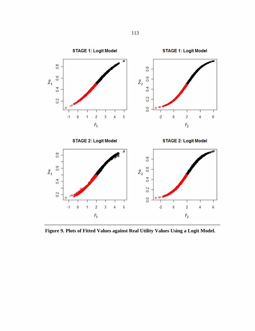
113
Figure 9. Plots of Fitted Values against Real Utility Values Using a Logit Model.
114
Figure 10. Plots of Fitted Values against Real Utility Values Using a Tobit Model.

115
APPENDIX C
CODE
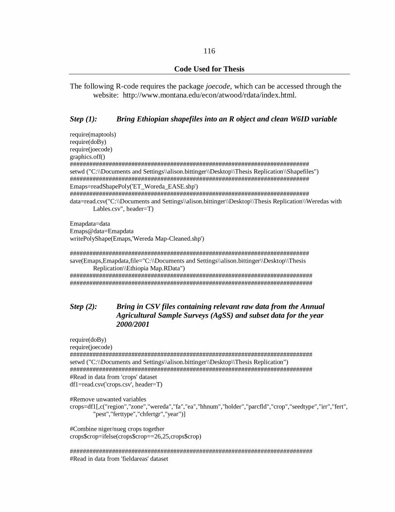
116
Code Used for Thesis
The following R-code requires the package joecode, which can be accessed through the
website: http://www.montana.edu/econ/atwood/rdata/index.html.
Step (1): Bring Ethiopian shapefiles into an R object and clean W6ID variable
require(maptools)
require(doBy)
require(joecode)
graphics.off()
########################################################################## setwd ("C:\\Documents and Settings\\alison.bittinger\\Desktop\\Thesis Replication\\Shapefiles")
##########################################################################
Emaps=readShapePoly('ET_Woreda_EASE.shp')
##########################################################################
data=read.csv("C:\\Documents and Settings\\alison.bittinger\\Desktop\\Thesis Replication\\Weredas with
Lables.csv", header=T)
Emapdata=data
Emaps@data=Emapdata
writePolyShape(Emaps,'Wereda Map-Cleaned.shp')
##########################################################################
save(Emaps,Emapdata,file="C:\\Documents and Settings\\alison.bittinger\\Desktop\\Thesis
Replication\\Ethiopia Map.RData")
###########################################################################
###########################################################################
Step (2): Bring in CSV files containing relevant raw data from the Annual
Agricultural Sample Surveys (AgSS) and subset data for the year
2000/2001
require(doBy)
require(joecode)
###########################################################################
setwd ("C:\\Documents and Settings\\alison.bittinger\\Desktop\\Thesis Replication")
###########################################################################
#Read in data from 'crops' dataset
df1=read.csv('crops.csv', header=T)
#Remove unwanted variables crops=df1[,c("region","zone","wereda","fa","ea","hhnum","holder","parcfld","crop","seedtype","irr","fert",
"pest","ferttype","chfertgr","year")]
#Combine niger/nueg crops together
crops$crop=ifelse(crops$crop==26,25,crops$crop)
###########################################################################
#Read in data from 'fieldareas' dataset
117
df2=read.csv('fieldareas.csv', header=T)
#Remove unwanted variables
areas=df2[,c("region","zone","wereda","fa","ea","hhnum","holder","parcfld","crop","areacalc","year")]
#Combine niger/nueg crops together areas$crop=ifelse(areas$crop==26,25,areas$crop)
#Convert m^2 to hectares
areas$areacalc=areas$areacalc/10000
###########################################################################
#Read in data from 'holders' dataset
df3=read.csv('holders.csv', header=T)
#Remove unwanted variables
holders=df3[,c("region","zone","wereda","fa","ea","hhnum","holder","sex","age","ed","hhsize","year")]
############################################################################
#Read in data from 'cropcodes' dataset
cropcodes=read.csv("Crop Codes.csv", header=T)
############################################################################
memory.limit(3072)
#Merge four datasets together
df4=merge(crops, areas)
df5=merge(holders, df4)
AgSS=merge(cropcodes, df5)
#Create region ID
AgSS$R2ID=AgSS$region
AgSS$R2ID=as.character(AgSS$R2ID)
AgSS$R2ID=as.numeric(AgSS$R2ID)
#Create zone ID
AgSS$Z4ID=AgSS$R2ID*100+AgSS$zone
AgSS$Z4ID=as.character(AgSS$Z4ID)
AgSS$Z4ID=as.numeric(AgSS$Z4ID)
#Create wereda ID
AgSS$W6ID=AgSS$Z4ID*100+AgSS$wereda
AgSS$W6ID=as.character(AgSS$W6ID)
AgSS$W6ID=as.numeric(AgSS$W6ID)
#Create FA ID
AgSS$F9ID=AgSS$W6ID*1000+AgSS$fa
AgSS$F9ID=as.character(AgSS$F9ID)
AgSS$F9ID=as.numeric(AgSS$F9ID)
#Create EA ID
AgSS$E11ID=AgSS$F9ID*100+AgSS$ea AgSS$E11ID=as.character(AgSS$E11ID)
118
AgSS$E11ID=as.numeric(AgSS$E11ID)
#Create holder ID
AgSS$H16ID=AgSS$E11ID*100000+AgSS$hhnum*100+AgSS$holder
AgSS$H16ID=as.character(AgSS$H16ID)
AgSS$H16ID=as.numeric(AgSS$H16ID)
###########################################################################
#Change binary variables to 0/1
AgSS$sex2=ifelse(AgSS$sex==1,1,0)
AgSS$fert2=ifelse(AgSS$fert==1,1,0)
AgSS$irr2=ifelse(AgSS$irr==1,1,0)
AgSS$pest2=ifelse(AgSS$pest==1,1,0)
AgSS$seedtype2=ifelse(AgSS$seedtype==1,1,0)
############################################################################
AgSS2=AgSS[,c("R2ID","Z4ID","W6ID","F9ID","E11ID","H16ID","year","age","ed","sex2","hhsize","pa
rcfld","crop","cname","class","yield","fert2","ferttype","chfertgr","seedtype2","irr2","pest2","areacalc")]
############################################################################
save(AgSS2, file="AgSS.RData")
############################################################################
#Subset the data to exclude region 6 (Benishangul Gumuz)
tmp1=subset(AgSS2, R2ID!=6)
#Subset the data for the year 2000/2001
AgSS2000=subset(tmp1, tmp1$year==0001)
############################################################################
save(AgSS2000, file="AgSS2000.RData")
############################################################################
############################################################################
Step (3): Create crop category revenue estimates for each region require(doBy) require(joecode) ############################################################################ setwd ("C:\\Documents and Settings\\alison.bittinger\\Desktop\\Thesis Replication") ############################################################################ load('AgSS2000.RData') ############################################################################ #Sum area by crop and R2ID tmp2=summaryBy(areacalc~crop+R2ID, data=AgSS2000, FUN=sum, na.rm=T) names(tmp2)[3]='croparea' #Bring in yield data tmp3=AgSS2000[,c("cname","crop","yield")] tmp4=unique(tmp3) #Merge yield data with crop areas
119
tmp5=merge(tmp4,tmp2) #Create production estimates tmp5$prod=tmp5$yield*tmp5$croparea ############################################################################# #Read in data from 'Crop Prices' dataset cropprices=read.csv("Crop Prices.csv", header=T) names(cropprices) # "R2ID" "crop" "cprice" "class" ############################################################################## #Merge production and prices data to form revenue estimates (birr/m2) by crops rev=merge(cropprices, tmp5) names(rev) #[1] "R2ID" "crop" "cprice" "class" "cname" "yield" #[7] "croparea" "prod" #Create income estimates rev$income=rev$cprice*rev$prod #Create revenue/area estimates rev$revest=rev$income/rev$croparea #Remove missing values rev1=rev[!is.na(rev$revest),] dfa1=rev1[,c("R2ID","crop","class","revest")] ################################################################################ #Create relative regional revenue/m2 estimates for crop categories tmp6=summaryBy(revest~R2ID+class, data=dfa1, FUN=mean, na.rm=T) names(tmp6)[3]="revclass" tmp7=summaryBy(revclass~R2ID, data=tmp6, FUN=mean) names(tmp7)[2]="avgrevclass" tmp8=merge(tmp7, tmp6) tmp8$relrev=tmp8$revclass/tmp8$avgrevclass ################################################################################# #Seperate into classification revenue estimation variables df11=subset(tmp8, class==1) df11=df11[,c("R2ID", "relrev")] names(df11)=c("R2ID","rev1") df12=subset(tmp8, class==2) df12=df12[,c("R2ID", "relrev")] names(df12)=c("R2ID","rev2")
120
df13=subset(tmp8, class==3) df13=df13[,c("R2ID", "relrev")] names(df13)=c("R2ID","rev3") df14=subset(tmp8, class==4) df14=df14[,c("R2ID", "relrev")] names(df14)=c("R2ID","rev4") df15=subset(tmp8, class==5) df15=df15[,c("R2ID", "relrev")] names(df15)=c("R2ID","rev5") #Merge classpct dataframes df1=merge(df11, df12, all.x=T, all.y=T) df2=merge(df1, df13, all.x=T, all.y=T) df3=merge(df2, df14, all.x=T, all.y=T) df4=merge(df3, df15, all.x=T, all.y=T) #Convert NA values to 0s df4$rev1=ifelse(is.na(df4$rev1),0,df4$rev1) #################################################################################### #Merge revclass estimates with crop revenue estimates dfa2=merge(dfa1, df4) #################################################################################### #Form overall revenue estimates dataframe RevEst=dfa2[,c("R2ID","crop","class","revest","rev1","rev2","rev3","rev4","rev5")] #################################################################################### save(RevEst, file="Revenue Estimates.RData") #################################################################################### ####################################################################################
Step (4): Aggregate 2000/2001 data to a farmer level with teff classified as the primary staple crop; create Herfindahl Index (HHI) and Crop Category Shares
require(joecode) require(doBy) #################################################################################### setwd ("C:\\Documents and Settings\\alison.bittinger\\Desktop\\Thesis Replication") #################################################################################### load("AgSS2000.RData") #################################################################################### #Remove missing values AgSS2000.1=AgSS2000[!is.na(AgSS2000$pest),] AgSS2000.2=AgSS2000.1[!is.na(AgSS2000.1$fert2),] AgSS2000.3=AgSS2000.2[!is.na(AgSS2000.2$seedtype2),]
121
AgSS2000.4=subset(AgSS2000.3, !(fert2>0&is.na(ferttype))) AgSS2000.4$ferttype=ifelse(is.na(AgSS2000.4$ferttype),0, AgSS2000.4$ferttype) AgSS2000.5=subset(AgSS2000.4, !(fert2==0&ferttype>0)) #Currently, ferttype = 0 (no fert); ferttype = 1 (natural fert); ferttype = 2 (chem fert); ferttype = 3 (both
natural and chem fert) #Change ferttype variable into binary so that no fertilizer & natural fertilizer = 0 and chemical fertilizer or
both natural and chemical fertilizer = 1 AgSS2000.5$ferttype=ifelse(AgSS2000.5$ferttype>1,1,0) ##################################################################################### #SUMMARIZE INPUT USE BY FARMERS ##################################################################################### #Calculate area cultivated by each farmer area=summaryBy(areacalc~H16ID, data=AgSS2000.5, FUN=sum, na.rm=T) names(area)[2]='areacult' ###################################################################################### #Summarize fertilizer use by farmer #Calculate total area devoted to fertilizers by farmer f1=summaryBy(areacalc~H16ID+ferttype, data=AgSS2000.5, FUN=sum, na.rm=T) #Seperate areas by fertilizer type f10=subset(f1, ferttype==0) names(f10) = c("H16ID","nocfert","area_nocfert") f10=f10[,c("H16ID","area_nocfert")] f11=subset(f1, ferttype==1) names(f11) = c("H16ID","cfert","area_cfert") f11=f11[,c("H16ID","area_cfert")] #Merge fertilizer use data f2=merge(f10, f11, all.x=T, all.y=T) f3=merge(f2, area) f3$area_nocfert=ifelse(is.na(f3$area_nocfert),0,f3$area_nocfert) f3$area_cfert=ifelse(is.na(f3$area_cfert),0,f3$area_cfert) #Find shares of area devoted to no chemical fertilizer and/or chemical fertilizer f3$nocfert=f3$area_nofert/f3$areacult f3$cfert=f3$area_cfert/f3$areacult #Summarize chemical fertilizer usage by farmer (calculate length and sum) f4=summaryDF(AgSS2000.5, c('H16ID'),c('ferttype', 'ferttype'), c('length', 'sum')) #Calculate average chemical fertilizer use by farmer (now a continuous variable) f4$avgcfert=f4$ferttype.1.sum/f4$ferttype.length #Convert to question, Did you use any chemical fertilizer on any of your fields (Y/N)?
122
f4$Acfert=ifelse(f4$avgcfert==0,0,1) #Summarize fertilizer usage by farmer (yes/no) f5=summaryDF(AgSS2000.5, c('H16ID'),c('fert2', 'fert2'), c('length', 'sum')) #Calculate average fertilizer use by farmer (now a continuous variable) f5$avgfert=f5$fert2.1.sum/f5$fert2.length #Convert to question, Did you use fertilizer on any of your fields (Y/N)? f5$Afert=ifelse(f5$avgfert==0,0,1) f6=merge(f3,f4) f7=merge(f6,f5) fert=f7[,c("H16ID","cfert","Acfert","ferttype.length","Afert")] names(fert)[4]='fieldnum' ################################################################################# #Summarize irrigation use by farmer #Calculate total area devoted to irrigation by farmer i1=summaryBy(areacalc~H16ID+irr2, data=AgSS2000.5, FUN=sum, na.rm=T) #Seperate areas by irrigation type i10=subset(i1, irr2==0) names(i10) = c("H16ID","noirr","area_noirr") i10=i10[,c("H16ID","area_noirr")] i11=subset(i1, irr2==1) names(i11) = c("H16ID","irr","area_irr") i11=i11[,c("H16ID","area_irr")] #Merge irrigation use data i2=merge(i10, i11, all.x=T, all.y=T) i3=merge(i2, area) i3$area_noirr=ifelse(is.na(i3$area_noirr),0,i3$area_noirr) i3$area_irr=ifelse(is.na(i3$area_irr),0,i3$area_irr) #Find shares of area devoted to no irrigation and/or irrigation i3$noirr=i3$area_noirr/i3$areacult i3$irr=i3$area_irr/i3$areacult #Summarize irrigation usage by farmer (calculate length and sum) i4=summaryDF(AgSS2000.5, c('H16ID'),c('irr2', 'irr2'), c('length', 'sum')) #Calculate average irrigation use by farmer (now a continuous variable) i4$avgirr=i4$irr2.1.sum/i4$irr2.length #Convert to question, Did you use any irrigation on any of your fields (Y/N)? i4$Airr=ifelse(i4$avgirr==0,0,1)

123
i5=merge(i3,i4) irr=i5[,c("H16ID","irr","Airr")] ################################################################################# #Summarize pesticides use by farmer ################################################################################# #Calculate total area devoted to pesticides by farmer p1=summaryBy(areacalc~H16ID+pest2, data=AgSS2000.5, FUN=sum, na.rm=T) #Seperate areas by pesticides type p10=subset(p1, pest2==0) names(p10) = c("H16ID","nopest","area_nopest") p10=p10[,c("H16ID","area_nopest")] p11=subset(p1, pest2==1) names(p11) = c("H16ID","pest","area_pest") p11=p11[,c("H16ID","area_pest")] #Merge pesticides use data p2=merge(p10, p11, all.x=T, all.y=T) p3=merge(p2, area) p3$area_nopest=ifelse(is.na(p3$area_nopest),0,p3$area_nopest) p3$area_pest=ifelse(is.na(p3$area_pest),0,p3$area_pest) #Find shares of area devoted to no pesticides and/or pesticides p3$nopest=p3$area_nopest/p3$areacult p3$pest=p3$area_pest/p3$areacult #Summarize pesticides usage by farmer (calculate length and sum) p4=summaryDF(AgSS2000.5, c('H16ID'),c('pest2', 'pest2'), c('length', 'sum')) #Calculate average pesticides use by farmer (now a continuous variable) p4$avgpest=p4$pest2.1.sum/p4$pest2.length #Convert to question, Did you use any pesticides on any of your fields (Y/N)? p4$Apest=ifelse(p4$avgpest==0,0,1) p5=merge(p3,p4) pest=p5[,c("H16ID","pest","Apest")] ############################################################################## #Summarize improved seed use by farmer #Calculate total area devoted to improved seed by farmer s1=summaryBy(areacalc~H16ID+seedtype2, data=AgSS2000.5, FUN=sum, na.rm=T) #Seserate areas by improved seed tyse s10=subset(s1, seedtype2==0) names(s10) = c("H16ID","noseed","area_noseed")
124
s10=s10[,c("H16ID","area_noseed")] s11=subset(s1, seedtype2==1) names(s11) = c("H16ID","seed","area_seed") s11=s11[,c("H16ID","area_seed")] #Merge improved seed use data s2=merge(s10, s11, all.x=T, all.y=T) s3=merge(s2, area) s3$area_noseed=ifelse(is.na(s3$area_noseed),0,s3$area_noseed) s3$area_seed=ifelse(is.na(s3$area_seed),0,s3$area_seed) #Find shares of area devoted to no improved seed and/or improved seed s3$noseed=s3$area_noseed/s3$areacult s3$seed=s3$area_seed/s3$areacult #Summarize improved seed usage by farmer (calculate length and sum) s4=summaryDF(AgSS2000.5, c('H16ID'),c('seedtype2', 'seedtype2'), c('length', 'sum')) #Calculate average improved seed use by farmer (now a continuous variable) s4$avgseed=s4$seedtype2.1.sum/s4$seedtype2.length #Convert to question, Did you use any improved seed on any of your fields (Y/N)? s4$Aseed=ifelse(s4$avgseed==0,0,1) s5=merge(s3,s4) seed=s5[,c("H16ID","seed","Aseed")] ################################################################################## #Merge all inputs inputs1=merge(fert,irr) inputs2=merge(inputs1,pest) inputs=merge(inputs2,seed) ################################################################################## #Calculating the Herfindahl Index -- Diversification Measure ################################################################################## #Sums the area of parcel/fields for each crop by holder and merges both sums div1=summaryBy(areacalc~H16ID+crop, data=AgSS2000.5, FUN=sum, keep.names=T, na.rm=T) div2=merge(div1,area, all.x=T) #Calculates the area represented by each crop in a year as a percentage div2$croppct=div2$areacalc/div2$areacult #Square the crop shares div2$croppct2=div2$croppct*div2$croppct #Create the HHI by summing each crop share by holder div3=summaryBy(croppct2~H16ID, data=div2, FUN=sum, na.rm=T)
125
divers=merge(div3,div2) names(divers)[2]="HHI" names(divers)[4]="areacalc.crop" ################################################################################### #Calculate Crop Shares by Crop Categories ################################################################################### #Sum the acreage for each holder by classification shr1=summaryBy(areacalc~H16ID+class, data=AgSS2000.5, FUN=sum, na.rm=T) names(shr1)[3]="areaclass" shr2=merge(shr1, area) #Calculate the acreage share represented by each crop classification for each holder shr2$classpct=shr2$areaclass/shr2$areacult #Only keep necessary variables shr3=shr2[,c("H16ID","class","classpct")] #Seperate into classification share variables tmp11=subset(shr3, class==1) names(tmp11)=c("H16ID","class1","classpct1") tmp12=subset(shr3, class==2) names(tmp12)=c("H16ID","class2","classpct2") tmp13=subset(shr3, class==3) names(tmp13)=c("H16ID","class3","classpct3") tmp14=subset(shr3, class==4) names(tmp14)=c("H16ID","class4","classpct4") tmp15=subset(shr3, class==5) names(tmp15)=c("H16ID","class5","classpct5") #Merge classpct dataframes tmp1=merge(tmp11, tmp12, all.x=T, all.y=T) tmp2=merge(tmp1, tmp13, all.x=T, all.y=T) tmp3=merge(tmp2, tmp14, all.x=T, all.y=T) tmp4=merge(tmp3, tmp15, all.x=T, all.y=T) #Convert NA values to 0s tmp4$classpct1=ifelse(is.na(tmp4$classpct1),0,tmp4$classpct1) tmp4$classpct2=ifelse(is.na(tmp4$classpct2),0,tmp4$classpct2) tmp4$classpct3=ifelse(is.na(tmp4$classpct3),0,tmp4$classpct3) tmp4$classpct4=ifelse(is.na(tmp4$classpct4),0,tmp4$classpct4) tmp4$classpct5=ifelse(is.na(tmp4$classpct5),0,tmp4$classpct5) #################################################################################### #Calculate Major Crop Produced by each Household

126
#################################################################################### cat=NULL holderlist=sort(unique(AgSS2000.5$H16ID)) id=1 for(id in 1:length(holderlist)){ #start loop on Holder ID (holder=holderlist[id]) cat1=subset(shr3, H16ID==holder) cat2=orderBy(~-classpct, data=cat1) cat2$major=cat2$class[1] cat3=unique(cat2[,c("H16ID","major")]) cat=rbind(cat,cat3) } #end loop on Holder ID cat=data.frame(cat) #Convert Major Crop Categories into dummy variables cat$sub=ifelse(cat$major==1,1,0) cat$cer=ifelse(cat$major==2,1,0) cat$oil=ifelse(cat$major==3,1,0) cat$fruit=ifelse(cat$major==4,1,0) cat$cash=ifelse(cat$major==5,1,0) ################################################################################### #Only keep unique and necessary variables for merger #Variables related to input use dfa1=inputs dfa2=unique(dfa1) #Variables related to diversification dfa3=divers[,c("H16ID","areacult","HHI")] dfa4=unique(dfa3) #Variables related to classification shares dfa5=tmp4[,c("H16ID","classpct1","classpct2","classpct3","classpct4","classpct5")] dfa6=unique(dfa5) #Variables related to predominant crops dfa7=cat[,c("H16ID","sub","cer","oil","fruit","cash")] dfa8=unique(dfa7) ################################################################################### #Merge all aggregate characteristics together tmp5=merge(dfa2, dfa4) tmp6=merge(dfa6,tmp5) tmp7=merge(dfa8,tmp6)
127
farms2000=tmp7[,c("H16ID","areacult","fieldnum","HHI","classpct1","classpct2","classpct3","classpct4","classpct5","sub","cer","oil","fruit","cash","cfert","Acfert","Afert","irr","Airr","pest","Apest","seed","Aseed")]
#################################################################################### save(farms2000, file='Farms 2000.RData') demo2000=AgSS2000.5[,c("R2ID","Z4ID","W6ID","F9ID","E11ID","H16ID","sex2","age","ed","hhsize")] #Merge Farm Aggregate Characteristics with Farmer Demographics dfa9=merge(demo2000,farms2000) farmer2000=unique(dfa9) save(farmer2000, file='Farmer 2000.RData') #################################################################################### ####################################################################################
Step (5): Subset World Bank/European Commission World Map of Travel Time to Horn of Africa
require(joecode) require(R.matlab) require(doBy) require(maps) ##################################################################################### setwd("C:\\Documents and Settings\\alison.bittinger\\Desktop\\Thesis Replication\\World Traveltime") ##################################################################################### df1=read.table('acc_50k_200000bak_subset_30_50e_0_20n.dat',header=T) df1[df1>=100000]=NA df1=orderBy(~long+lat,data=df1) summary(df1) tmp=colorum.gplots(df1$val,scoremax=2000,Lround=0) df1$color=tmp$datacolors plot(30:50,0:20,type='n') x=sort(unique(df1$long)) xlong=30 for(xlong in 30:50){ xm1=xlong-1 df2=df1[df1$long>xm1&df1$long<=xlong,] points(df2$long,df2$lat,col=df2$color,pch=20,cex=0.25) } legend('bottomright',legend=tmp$Ltext,fill=tmp$Lcolors,cex=0.5) map('world',add=T,lwd=2)
128
save(df1,file="C:\\Documents and Settings\\alison.bittinger\\Desktop\\Thesis Replication\\TTime - Horn of Africa.RData")
############################################################################### ###############################################################################
Step (6): Create average travel time variable require(maptools) require(joecode) require(doBy) graphics.off() ############################################################################### setwd("C:\\Documents and Settings\\alison.bittinger\\Desktop\\Thesis Replication") ############################################################################### #Bring in Ethiopian Shapefiles load("Ethiopia Map.RData") plot(Emaps) ############################################################################### #Bring in Travel Time Pixelated Data load("TTime - Horn of Africa.RData") ############################################################################### memory.limit(3072) ############################################################################### #OVERLAY FUNCTION: Reduce time travel data to Ethiopia ############################################################################### #Convert travel time data into a spatial object df2=df1 coordinates(df2)=~long+lat index=overlay(df2,Emaps) df1$index=index df1[1:10,] #Reduce time travel data to only Ethiopia df3=subset(df1,!is.na(index)) save(df1, df3, Emaps, Emapdata, file="Ethiopia TTime.RData") ################################################################################# #Create distance from market by wereda variable ################################################################################# #Sum areas for weredas on map that are represented by multiple areas dfa=summaryBy(Area_km2~W6ID, data=Emapdata, FUN=sum, keep.names=T) #Problem with multiple coding in original map data Emapdata$Map_W6ID[339]=40121 dfa2=Emapdata[,c("W6ID","W_NAME","Z4ID","Z_NAME","R2ID","R_NAME","index","Map_W6ID")] dfa3=merge(dfa, dfa2, all.x=T)

129
#Find a mean isolation measure for each wereda df4=summaryDF(df3,c("index"),c("val"),c("mean")) names(df4)[2]="w_dist" ################################################################################### #Merge isolation variable with Emapdata df5=merge(dfa3, df4, all.x=T) #Find mean travel time for weredas on map that are represented by multiple areas df6=summaryBy(w_dist~W6ID, data=df5, FUN=mean, keep.names=T) df7=df5[,c("W6ID","W_NAME","Z4ID","Z_NAME","R2ID","R_NAME","Area_km2","Map_W6ID","index")] df8=merge(df6, df7) #Convert distance to hours df8$w_dist = df8$w_dist/60 #Convert area to hectares df8$Area_km2 = df8$Area_km2*100 df9=unique(df8) save(df9, Emaps, file="Avg Wereda TTime.RData") #################################################################################### ####################################################################################
Step (7): Create finance variables require(joecode) require(doBy) #################################################################################### setwd("C:\\Documents and Settings\\alison.bittinger\\Desktop\\Thesis Replication\\Finance Data") #################################################################################### codes=read.csv("Wereda-Town Codes.csv", header=T) micro=read.csv("Microfinance Institutions.csv", header=T) banks=read.csv("Banks.csv", header=T) ################################################################################## #Find microfinance institution counts tmp=merge(codes, micro, all.x=T) micro1=summaryBy(MFI_NAME~Map_W6ID, data=tmp, FUN=length) names(micro1)[2]="w_inst" #Create complete bank counts tmp1=merge(codes, banks, all.x=T) tmp1$w_banks=ifelse(is.na(tmp1$w_banks),0,tmp1$w_banks) tmp2=tmp1[,c("Map_W6ID","w_banks")]
130
tmp2=unique(tmp2) #Merge institutions and banks fin=merge(micro1, tmp2, all.x=T) save(fin, file="C:\\Documents and Settings\\alison.bittinger\\Desktop\\Thesis
Replication\\Finance.RData") ################################################################################## ##################################################################################
Step (8): Create a dataset with wereda-specific variables require(doBy) require(joecode) ################################################################################## setwd ("C:\\Documents and Settings\\alison.bittinger\\Desktop\\Thesis Replication") ################################################################################## bio=read.csv("Biophysical.csv", header=T) pop=read.csv("Population.csv", header=T) load("Finance.RData") ################################################################################## #Merge finance, population, and biophysical variables tmp1=merge(bio, pop) tmp2=merge(tmp1, fin) tmp2$Map_W6ID=as.factor(tmp2$Map_W6ID) names(tmp2) # [1] "Map_W6ID" "avg_elev" "avg_slope" "avg_treecover" # [5] "avg_rainmonths" "roadden" "primschool" "secschool" # [9] "POP_DENS" "w_inst" "w_banks" names(tmp2)[2]="w_elev" names(tmp2)[3]="w_slope" names(tmp2)[4]="w_trees" names(tmp2)[5]="w_rainmo" names(tmp2)[6]="w_roadden" names(tmp2)[7]="w_primsch" names(tmp2)[8]="w_secsch" names(tmp2)[9]="w_popden" ################################################################################# load("Avg Wereda TTime.RData") ################################################################################# time=df9[,c("W6ID","w_dist","W_NAME","Z4ID","Z_NAME","R2ID","R_NAME","Area_km2","Map_W6ID")
] time1=unique(time) names(time1)[3]="w_name"
131
names(time1)[5]="z_name" names(time1)[7]="r_name" names(time1)[8]="w_area" time1$Map_W6ID=as.factor(time1$Map_W6ID) ############################################################################ #Merge travel time with wereda characteristics wereda=merge(time1, tmp2) ############################################################################ save(wereda, file="Wereda.RData") ############################################################################
Step (9): Create a master dataset that combines farmer, wereda-specific, and revenue data
require(doBy) require(joecode) ############################################################################ setwd ("C:\\Documents and Settings\\alison.bittinger\\Desktop\\Thesis Replication") ############################################################################ load("Revenue Estimates.RData") load("Farmer 2000.RData") load("Wereda.RData") ############################################################################ rev=RevEst[,c("R2ID","rev1","rev2","rev3","rev4","rev5")] rev2=unique(rev) ############################################################################ dfa1=merge(farmer2000, rev2) dfa2=merge(dfa1, wereda) ############################################################################ #Remove missing values dfa3=dfa2[!is.na(dfa2$w_primsch),] master=dfa3[!is.na(dfa3$w_popden),] ############################################################################ save(master, file="Master.RData") ############################################################################ ############################################################################
Step (11): Run chemical fertilizer and crop diversification simultaneous equation regressions
############################################################################ #Chemical Fertilizer and Diversification - Reduced Form Regressions ############################################################################

132
rm(list=ls()) set.seed(2010) ############################################################################ require(joecode) require(doBy) require(VGAM) ############################################################################ setwd("C:\\Documents and Settings\\alison.bittinger\\Desktop\\Thesis Replication\\Regressions") ############################################################################ load("Master.RData") ############################################################################ df1=master ############################################################################ #CHEMICAL FERTILIZER AS BINARY ADOPTION #OLS Estimation ols.chem1 =
lm(Acfert~HHI+w_dist+sex2+age+factor(ed)+hhsize+w_elev+w_slope+w_trees+w_rainmo+w_roadden+w_primsch+w_secsch+w_popden+w_banks+w_inst+Airr+areacult+fieldnum, data=df1)
#Simple Logit Estimation logit.chem1 =
glm(Acfert~HHI+w_dist+sex2+age+factor(ed)+hhsize+w_elev+w_slope+w_trees+w_rainmo+w_roadden+w_primsch+w_secsch+w_popden+w_banks+w_inst+Airr+areacult+fieldnum, binomial, data=df1)
############################################################################# #CHEMICAL FERTILIZER AS CONTINUOUS DIFFUSION #OLS Estimation ols.chem2 =
lm(cfert~HHI+w_dist+sex2+age+factor(ed)+hhsize+w_elev+w_slope+w_trees+w_rainmo+w_roadden+w_primsch+w_secsch+w_popden+w_banks+w_inst+Airr+areacult+fieldnum, data=df1)
ols.HHI = lm(HHI~cfert+w_dist+sex2+age+factor(ed)+hhsize+w_elev+w_slope+w_trees+w_rainmo+w_roadden+w_primsch+w_secsch+w_popden+w_banks+w_inst+Airr+w_area, data=df1)
#Simple Tobit Estimation tobit.chem2 =
vglm(cfert~HHI+w_dist+sex2+age+factor(ed)+hhsize+w_elev+w_slope+w_trees+w_rainmo+w_roadden+w_primsch+w_secsch+w_popden+w_banks+w_inst+Airr+areacult+fieldnum,tobit(Lower=0, Upper=1,zero=2), df1, trace=TRUE)
tobit.HHI = vglm(HHI~cfert+w_dist+sex2+age+factor(ed)+hhsize+w_elev+w_slope+w_trees+w_rainmo+w_roadden+w_primsch+w_secsch+w_popden+w_banks+w_inst+Airr+w_area,tobit(Upper=1,zero=2), df1, trace=TRUE)
############################################################################# #Simultaneous Equation Estimation #############################################################################
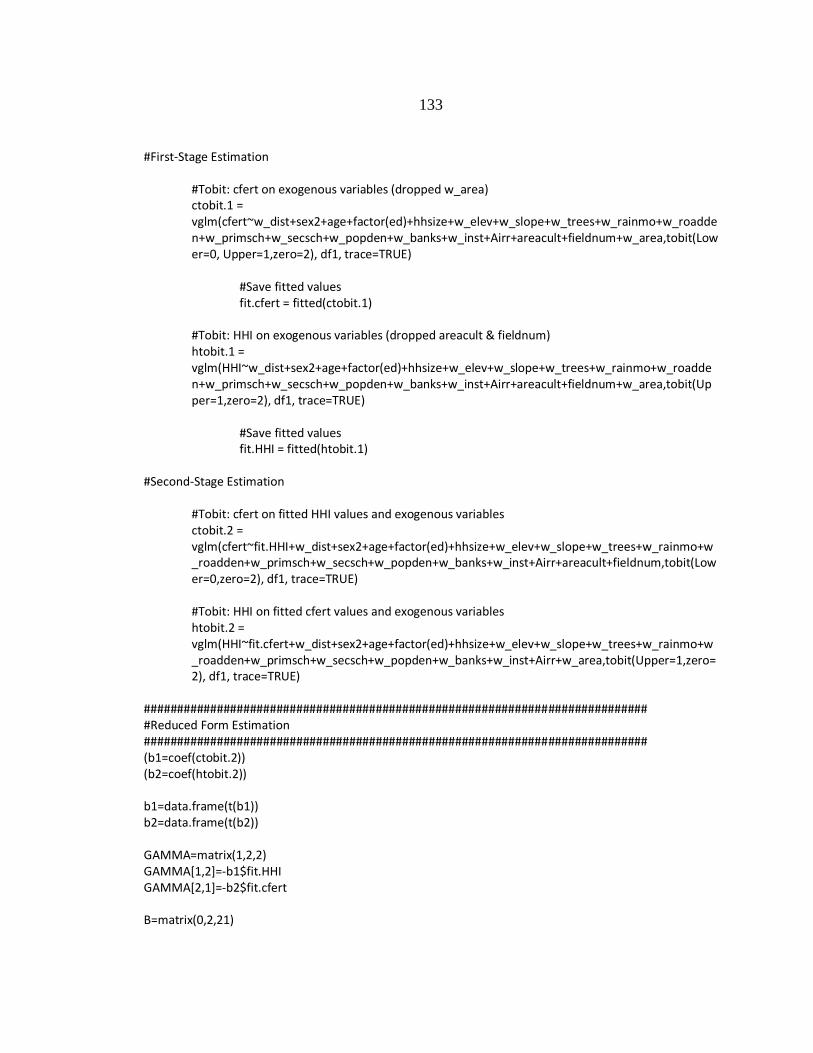
133
#First-Stage Estimation #Tobit: cfert on exogenous variables (dropped w_area) ctobit.1 =
vglm(cfert~w_dist+sex2+age+factor(ed)+hhsize+w_elev+w_slope+w_trees+w_rainmo+w_roadden+w_primsch+w_secsch+w_popden+w_banks+w_inst+Airr+areacult+fieldnum+w_area,tobit(Lower=0, Upper=1,zero=2), df1, trace=TRUE)
#Save fitted values fit.cfert = fitted(ctobit.1) #Tobit: HHI on exogenous variables (dropped areacult & fieldnum) htobit.1 =
vglm(HHI~w_dist+sex2+age+factor(ed)+hhsize+w_elev+w_slope+w_trees+w_rainmo+w_roadden+w_primsch+w_secsch+w_popden+w_banks+w_inst+Airr+areacult+fieldnum+w_area,tobit(Upper=1,zero=2), df1, trace=TRUE)
#Save fitted values fit.HHI = fitted(htobit.1) #Second-Stage Estimation #Tobit: cfert on fitted HHI values and exogenous variables ctobit.2 =
vglm(cfert~fit.HHI+w_dist+sex2+age+factor(ed)+hhsize+w_elev+w_slope+w_trees+w_rainmo+w_roadden+w_primsch+w_secsch+w_popden+w_banks+w_inst+Airr+areacult+fieldnum,tobit(Lower=0,zero=2), df1, trace=TRUE)
#Tobit: HHI on fitted cfert values and exogenous variables htobit.2 =
vglm(HHI~fit.cfert+w_dist+sex2+age+factor(ed)+hhsize+w_elev+w_slope+w_trees+w_rainmo+w_roadden+w_primsch+w_secsch+w_popden+w_banks+w_inst+Airr+w_area,tobit(Upper=1,zero=2), df1, trace=TRUE)
############################################################################ #Reduced Form Estimation ############################################################################ (b1=coef(ctobit.2)) (b2=coef(htobit.2)) b1=data.frame(t(b1)) b2=data.frame(t(b2)) GAMMA=matrix(1,2,2) GAMMA[1,2]=-b1$fit.HHI GAMMA[2,1]=-b2$fit.cfert B=matrix(0,2,21)
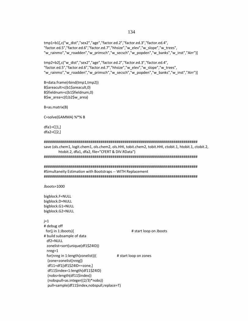
134
tmp1=b1[,c("w_dist","sex2","age","factor.ed.2","factor.ed.3","factor.ed.4", "factor.ed.5","factor.ed.6","factor.ed.7","hhsize","w_elev","w_slope","w_trees", "w_rainmo","w_roadden","w_primsch","w_secsch","w_popden","w_banks","w_inst","Airr")] tmp2=b2[,c("w_dist","sex2","age","factor.ed.2","factor.ed.3","factor.ed.4", "factor.ed.5","factor.ed.6","factor.ed.7","hhsize","w_elev","w_slope","w_trees", "w_rainmo","w_roadden","w_primsch","w_secsch","w_popden","w_banks","w_inst","Airr")] B=data.frame(rbind(tmp1,tmp2)) B$areacult=c(b1$areacult,0) B$fieldnum=c(b1$fieldnum,0) B$w_area=c(0,b2$w_area) B=as.matrix(B) C=solve(GAMMA) %*% B dfa1=C[1,] dfa2=C[2,] ############################################################################ save (ols.chem1, logit.chem1, ols.chem2, ols.HHI, tobit.chem2, tobit.HHI, ctobit.1, htobit.1, ctobit.2,
htobit.2, dfa1, dfa2, file="CFERT & DIV.RData") ############################################################################ ############################################################################ #Simultaneity Estimation with Bootstraps -- WITH Replacement ############################################################################ Jboots=1000 bigblock.F=NULL bigblock.D=NULL bigblock.G1=NULL bigblock.G2=NULL j=1 # debug off for(j in 1:Jboots){ # start loop on Jboots # build subsample of data df2=NULL zonelist=sort(unique(df1$Z4ID)) nreg=1 for(nreg in 1:length(zonelist)){ # start loop on zones (zone=zonelist[nreg]) df11=df1[df1$Z4ID==zone,] df11$index=1:length(df11$Z4ID) (nobs=length(df11$index)) (nobspull=as.integer((2/3)*nobs)) pull=sample(df11$index,nobspull,replace=T)
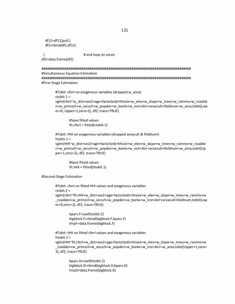
135
df12=df11[pull,] df2=rbind(df2,df12) } # end loop on zones df2=data.frame(df2) ############################################################################## #Simultaneous Equation Estimation ############################################################################## #First-Stage Estimation #Tobit: cfert on exogenous variables (dropped w_area) ctobit.1 =
vglm(cfert~w_dist+sex2+age+factor(ed)+hhsize+w_elev+w_slope+w_trees+w_rainmo+w_roadden+w_primsch+w_secsch+w_popden+w_banks+w_inst+Airr+areacult+fieldnum+w_area,tobit(Lower=0, Upper=1,zero=2), df2, trace=TRUE)
#Save fitted values fit.cfert = fitted(ctobit.1) #Tobit: HHI on exogenous variables (dropped areacult & fieldnum) htobit.1 =
vglm(HHI~w_dist+sex2+age+factor(ed)+hhsize+w_elev+w_slope+w_trees+w_rainmo+w_roadden+w_primsch+w_secsch+w_popden+w_banks+w_inst+Airr+areacult+fieldnum+w_area,tobit(Upper=1,zero=2), df2, trace=TRUE)
#Save fitted values fit.HHI = fitted(htobit.1) #Second-Stage Estimation #Tobit: cfert on fitted HHI values and exogenous variables ctobit.2 =
vglm(cfert~fit.HHI+w_dist+sex2+age+factor(ed)+hhsize+w_elev+w_slope+w_trees+w_rainmo+w_roadden+w_primsch+w_secsch+w_popden+w_banks+w_inst+Airr+areacult+fieldnum,tobit(Lower=0,zero=2), df2, trace=TRUE)
bpars.F=coef(ctobit.2) bigblock.F=rbind(bigblock.F,bpars.F) tmpF=data.frame(bigblock.F) #Tobit: HHI on fitted cfert values and exogenous variables htobit.2 =
vglm(HHI~fit.cfert+w_dist+sex2+age+factor(ed)+hhsize+w_elev+w_slope+w_trees+w_rainmo+w_roadden+w_primsch+w_secsch+w_popden+w_banks+w_inst+Airr+w_area,tobit(Upper=1,zero=2), df2, trace=TRUE)
bpars.D=coef(htobit.2) bigblock.D=rbind(bigblock.D,bpars.D) tmpD=data.frame(bigblock.D)

136
############################################################################## #Reduced Form Estimation ############################################################################## (B1=coef(ctobit.2)) (B2=coef(htobit.2)) B1=data.frame(t(B1)) B2=data.frame(t(B2)) DELTA=matrix(1,2,2) DELTA[1,2]=-B1$fit.HHI DELTA[2,1]=-B2$fit.cfert E=matrix(0,2,21) tmp3=B1[,c("w_dist","sex2","age","factor.ed.2","factor.ed.3","factor.ed.4", "factor.ed.5","factor.ed.6","factor.ed.7","hhsize","w_elev","w_slope","w_trees", "w_rainmo","w_roadden","w_primsch","w_secsch","w_popden","w_banks","w_inst","Airr")] tmp4=B2[,c("w_dist","sex2","age","factor.ed.2","factor.ed.3","factor.ed.4", "factor.ed.5","factor.ed.6","factor.ed.7","hhsize","w_elev","w_slope","w_trees", "w_rainmo","w_roadden","w_primsch","w_secsch","w_popden","w_banks","w_inst","Airr")] E=data.frame(rbind(tmp3,tmp4)) E$areacult=c(B1$areacult,0) E$fieldnum=c(B1$fieldnum,0) E$w_area=c(0,B2$w_area) E=as.matrix(E) G=solve(DELTA) %*% E dfa3=G[1,] dfa4=G[2,] bigblock.G1=rbind(bigblock.G1,dfa3) tmpG1=data.frame(bigblock.G1) bigblock.G2=rbind(bigblock.G2,dfa4) tmpG2=data.frame(bigblock.G2) } # end loop on Jboots ################################################################################# save (tmpF,tmpD,tmpG1,tmpG2, file="CFERT & DIV - Bootstrap.RData") ################################################################################# #Find P-Values of Bootstrapped Regressions Pval=function(b){ b0=mean(b) if(b0<=0){ tmp=b[b>=0]}
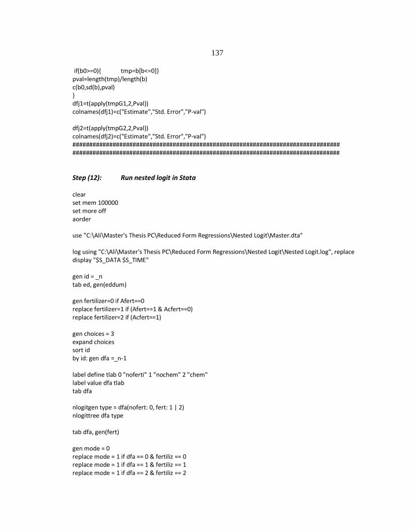
137
if(b0>=0){ tmp=b[b<=0]} pval=length(tmp)/length(b) c(b0,sd(b),pval) } dfj1=t(apply(tmpG1,2,Pval)) colnames(dfj1)=c("Estimate","Std. Error","P-val") dfj2=t(apply(tmpG2,2,Pval)) colnames(dfj2)=c("Estimate","Std. Error","P-val") ################################################################################ ################################################################################
Step (12): Run nested logit in Stata clear set mem 100000 set more off aorder use "C:\Ali\Master's Thesis PC\Reduced Form Regressions\Nested Logit\Master.dta" log using "C:\Ali\Master's Thesis PC\Reduced Form Regressions\Nested Logit\Nested Logit.log", replace display "$S_DATA $S_TIME" gen id = _n tab ed, gen(eddum) gen fertilizer=0 if Afert==0 replace fertilizer=1 if (Afert==1 & Acfert==0) replace fertilizer=2 if (Acfert==1) gen choices = 3 expand choices sort id by id: gen dfa =_n-1 label define tlab 0 "noferti" 1 "nochem" 2 "chem" label value dfa tlab tab dfa nlogitgen type = dfa(nofert: 0, fert: 1 | 2) nlogittree dfa type tab dfa, gen(fert) gen mode = 0 replace mode = 1 if dfa == 0 & fertiliz == 0 replace mode = 1 if dfa == 1 & fertiliz == 1 replace mode = 1 if dfa == 2 & fertiliz == 2
138
aorder global df1 HHI w_dist sex2 age eddum2 eddum3 eddum4 eddum5 eddum6 eddum7 hhsize w_elev
w_slope w_trees w_rainmo w_roadden /// w_primsch w_secsch w_popden w_banks w_inst Airr areacult fieldnum /*Nested Logit on All Exogenous Variables*/ nlogit mode || type: $df1, base(nofert) || dfa:, case(id) log close ################################################################################ ################################################################################
Step (13): Run crop categories regressions require(joecode) require(doBy) require(VGAM) ################################################################################ setwd("C:\\Ali\\Master's Thesis PC\\Reduced Form Regressions") #TEFF IS CATEGORIZED AS THE PRIMARY STAPLE CROP ################################################################################ load("Master.RData") ################################################################################ df1=master ################################################################################ #Singular Value Decomposition X=as.matrix(df1[,c("rev1", "rev2", "rev3", "rev4", "rev5")]) (d=svd(X)$d) (solve(t(X) %*% X)) max(d)/min(d) X=as.matrix(df1[,c("rev2", "rev4")]) (d=svd(X)$d) (solve(t(X) %*% X)) max(d)/min(d) ################################################################################ #OLS Estimation ################################################################################ #Estimation with technology factors based on adoption ols1 = lm(classpct1 ~ w_dist + rev2 + rev4 + sex2 + age + factor(ed) + fieldnum + Airr + hhsize + w_area +
w_banks + w_inst + w_popden + w_elev + w_slope + w_trees + w_rainmo + w_roadden + w_primsch + w_secsch, data=df1)
139
ols2 = lm(classpct2 ~ w_dist + rev2 + rev4 + sex2 + age + factor(ed) + fieldnum + Airr + hhsize + w_area + w_banks + w_inst + w_popden + w_elev + w_slope + w_trees + w_rainmo + w_roadden + w_primsch + w_secsch, data=df1)
ols3 = lm(classpct3 ~ w_dist + rev2 + rev4 + sex2 + age + factor(ed) + fieldnum + Airr + hhsize + w_area + w_banks + w_inst + w_popden + w_elev + w_slope + w_trees + w_rainmo + w_roadden + w_primsch + w_secsch, data=df1)
ols4 = lm(classpct4 ~ w_dist + rev2 + rev4 + sex2 + age + factor(ed) + fieldnum + Airr + hhsize + w_area + w_banks + w_inst + w_popden + w_elev + w_slope + w_trees + w_rainmo + w_roadden + w_primsch + w_secsch, data=df1)
ols5 = lm(classpct5 ~ w_dist + rev2 + rev4 + sex2 + age + factor(ed) + fieldnum + Airr + hhsize + w_area + w_banks + w_inst + w_popden + w_elev + w_slope + w_trees + w_rainmo + w_roadden + w_primsch + w_secsch, data=df1)
################################################################################ #Tobit Estimation ################################################################################ tobit1 = vglm(classpct1 ~ w_dist + rev2 + rev4 + fieldnum + sex2 + age + factor(ed) + Airr + hhsize +
w_area + w_banks + w_inst + w_popden + w_elev + w_slope + w_trees + w_rainmo + w_roadden + w_primsch + w_secsch, tobit(Lower=0, Upper=1, zero=2), df1, trace=TRUE)
tobit2 = vglm(classpct2 ~ w_dist + rev2 + rev4 + fieldnum + sex2 + age + factor(ed) + Airr + hhsize + w_area + w_banks + w_inst + w_popden + w_elev + w_slope + w_trees + w_rainmo + w_roadden + w_primsch + w_secsch, tobit(Lower=0, Upper=1, zero=2), df1, trace=TRUE)
tobit3 = vglm(classpct3 ~ w_dist + rev2 + rev4 + fieldnum + sex2 + age + factor(ed) + Airr + hhsize + w_area + w_banks + w_inst + w_popden + w_elev + w_slope + w_trees + w_rainmo + w_roadden + w_primsch + w_secsch, tobit(Lower=0, Upper=1, zero=2), df1, trace=TRUE)
tobit4 = vglm(classpct4 ~ w_dist + rev2 + rev4 + fieldnum + sex2 + age + factor(ed) + Airr + hhsize + w_area + w_banks + w_inst + w_popden + w_elev + w_slope + w_trees + w_rainmo + w_roadden + w_primsch + w_secsch, tobit(Lower=0, zero=2), df1, trace=TRUE)
tobit5 = vglm(classpct5 ~ w_dist + rev2 + rev4 + fieldnum + sex2 + age + factor(ed) + Airr + hhsize + w_area + w_banks + w_inst + w_popden + w_elev + w_slope + w_trees + w_rainmo + w_roadden + w_primsch + w_secsch, tobit(Lower=0, Upper=1, zero=2), df1, trace=TRUE)
############################################################################### save(ols1, ols2, ols3, ols4, ols5, tobit1, tobit2, tobit3, tobit4, tobit5, file="Crop Categories - Teff
(Primary).RData") ############################################################################### #TEFF IS CATEGORIZED AS A CEREAL CROP ############################################################################### load("Master - TRobust.RData") ############################################################################### df2=masterT ############################################################################### #OLS Estimation ############################################################################### #Estimation with technology factors based on adoption ols2.T = lm(classpct2 ~ w_dist + rev2 + rev4 + sex2 + age + factor(ed) + fieldnum + Airr + hhsize + w_area +
w_banks + w_inst + w_popden + w_elev + w_slope + w_trees + w_rainmo + w_roadden + w_primsch + w_secsch, data=df2)

140
ols3.T = lm(classpct3 ~ w_dist + rev2 + rev4 + sex2 + age + factor(ed) + fieldnum + Airr + hhsize + w_area + w_banks + w_inst + w_popden + w_elev + w_slope + w_trees + w_rainmo + w_roadden + w_primsch + w_secsch, data=df2)
ols4.T = lm(classpct4 ~ w_dist + rev2 + rev4 + sex2 + age + factor(ed) + fieldnum + Airr + hhsize + w_area + w_banks + w_inst + w_popden + w_elev + w_slope + w_trees + w_rainmo + w_roadden + w_primsch + w_secsch, data=df2)
ols5.T = lm(classpct5 ~ w_dist + rev2 + rev4 + sex2 + age + factor(ed) + fieldnum + Airr + hhsize + w_area + w_banks + w_inst + w_popden + w_elev + w_slope + w_trees + w_rainmo + w_roadden + w_primsch + w_secsch, data=df2)
############################################################################### #Tobit Estimation ############################################################################### tobit2.T = vglm(classpct2 ~ w_dist + rev2 + rev4 + fieldnum + sex2 + age + factor(ed) + Airr + hhsize +
w_area + w_banks + w_inst + w_popden + w_elev + w_slope + w_trees + w_rainmo + w_roadden + w_primsch + w_secsch, tobit(Lower=0, Upper=1, zero=2), df2, trace=TRUE)
tobit3.T = vglm(classpct3 ~ w_dist + rev2 + rev4 + fieldnum + sex2 + age + factor(ed) + Airr + hhsize + w_area + w_banks + w_inst + w_popden + w_elev + w_slope + w_trees + w_rainmo + w_roadden + w_primsch + w_secsch, tobit(Lower=0, Upper=1, zero=2), df2, trace=TRUE)
tobit4.T = vglm(classpct4 ~ w_dist + rev2 + rev4 + fieldnum + sex2 + age + factor(ed) + Airr + hhsize + w_area + w_banks + w_inst + w_popden + w_elev + w_slope + w_trees + w_rainmo + w_roadden + w_primsch + w_secsch, tobit(Lower=0, zero=2), df2, trace=TRUE)
tobit5.T = vglm(classpct5 ~ w_dist + rev2 + rev4 + fieldnum + sex2 + age + factor(ed) + Airr + hhsize + w_area + w_banks + w_inst + w_popden + w_elev + w_slope + w_trees + w_rainmo + w_roadden + w_primsch + w_secsch, tobit(Lower=0, Upper=1, zero=2), df2, trace=TRUE)
############################################################################### save(ols2.T, ols3.T, ols4.T, ols5.T, tobit2.T, tobit3.T, tobit4.T, tobit5.T, file="Crop Categories - Teff
(Cereal).RData") ############################################################################### ###############################################################################
Step (14): Visually check spatial correlation require(joecode) require(doBy) require(maptools) ################################################################################ setwd("C:\\Documents and Settings\\alison.bittinger\\Desktop\\Thesis Replication\\Regressions\\Spatial
Correlation") ################################################################################ load("Master.RData") load("Ethiopia Map.RData") ################################################################################ df3=master ################################################################################ #Simple OlS regression on Crop Categories, save residuals
141
ols1 = lm(classpct1 ~ w_dist + rev2 + rev4 + sex2 + age + factor(ed) + fieldnum + Airr + hhsize + w_area + w_banks + w_inst + w_popden + w_elev + w_slope + w_trees + w_rainmo + w_roadden + w_primsch + w_secsch, data=df3)
ols2 = lm(classpct2 ~ w_dist + rev2 + rev4 + sex2 + age + factor(ed) + fieldnum + Airr + hhsize + w_area + w_banks + w_inst + w_popden + w_elev + w_slope + w_trees + w_rainmo + w_roadden + w_primsch + w_secsch, data=df3)
ols3 = lm(classpct3 ~ w_dist + rev2 + rev4 + sex2 + age + factor(ed) + fieldnum + Airr + hhsize + w_area + w_banks + w_inst + w_popden + w_elev + w_slope + w_trees + w_rainmo + w_roadden + w_primsch + w_secsch, data=df3)
ols4 = lm(classpct4 ~ w_dist + rev2 + rev4 + sex2 + age + factor(ed) + fieldnum + Airr + hhsize + w_area + w_banks + w_inst + w_popden + w_elev + w_slope + w_trees + w_rainmo + w_roadden + w_primsch + w_secsch, data=df3)
ols5 = lm(classpct5 ~ w_dist + rev2 + rev4 + sex2 + age + factor(ed) + fieldnum + Airr + hhsize + w_area + w_banks + w_inst + w_popden + w_elev + w_slope + w_trees + w_rainmo + w_roadden + w_primsch + w_secsch, data=df3)
#Save residuals df3$ehat1=ols1$resid df3$ehat2=ols2$resid df3$ehat3=ols3$resid df3$ehat4=ols4$resid df3$ehat5=ols5$resid ################################################################################ #Plot OLS1 residuals on Ethiopia Map ################################################################################ #Summarize residuals by zone zres1=summaryBy(ehat1~Z4ID, data=df3, FUN=mean, keep.names=T) tmp2=merge(Emapdata, zres1, all.x=T) #Plot residuals by zone (blue/red) tmp2=orderBy(~index, data=tmp2) Ecolors=ifelse(tmp2$ehat1<0,'blue','red') x11() plot(Emaps,col=Ecolors,pch=20,cex=2) legend('bottomleft',"Negative Residual", fill='blue',cex=1) legend('topleft',"Positive Residual", fill='red',cex=1) #Plot residuals by zone (continuum) abehat1=abs(tmp2$ehat1) cmax2=quantile(abehat1,0.9,na.rm=T) temp=colorum.gplots(scores=tmp2$ehat1,Lround=3, scoremin=-cmax2, scoremax=cmax2, coL1=4,
coL2=0, coL3=2) x11() plot(Emaps,col=temp$datacolors,pch=20,cex=2) legend('topright',legend=temp$Ltext,fill=temp$Lcolors,cex=1) ############################################################################## ##############################################################################
142
Step (15): Create zone latitude/longitude measurements require(maptools) require(doBy) require(joecode) graphics.off() ############################################################################## setwd("C:\\Documents and Settings\\alison.bittinger\\Desktop\\Thesis Replication\\Regressions\\Spatial
Correlation") ############################################################################## wmaps=readShapePoly('Wereda Map-Cleaned.shp') plot(wmaps) ############################################################################## # pull the map attribute data wdata=wmaps@data graphics.off() ############################################################################### #Make backup objects wmaps2=wmaps wdata2=wmaps2@data #Create zonal lat-long values tmp=coordinates(wmaps2) wdata2$long=tmp[,1] wdata2$lat=tmp[,2] tmp2=summaryBy(long+lat~Z4ID,data=wdata2,FUN=mean,keep.names=T) tmp2=round(tmp2,4) write.csv(tmp2,file='longlat-zones.csv',row.names=F) #Compute distance between geometric centers of first two zones distcalc(tmp2$long[1],tmp2$lat[1],tmp2$long[2],tmp2$lat[2]) ############################################################################ ############################################################################
Step (16): Use simulation to check spatial correlation set.seed(2010) ############################################################################ require(joecode) require(maptools) require(doBy) ############################################################################

143
setwd("C:\\Documents and Settings\\alison.bittinger\\Desktop\\Thesis Replication\\Regressions\\Spatial Correlation")
############################################################################ load("Master.RData") longlat=read.csv("longlat-zones.csv", header=T) ############################################################################ df1=merge(master, longlat, all.x=T) ############################################################################# #Simple OlS regression on Crop Categories, save residuals ols1 = lm(classpct1 ~ w_dist + rev2 + rev4 + sex2 + age + factor(ed) + fieldnum + Airr + hhsize + w_area +
w_banks + w_inst + w_popden + w_elev + w_slope + w_trees + w_rainmo + w_roadden + w_primsch + w_secsch, data=df1)
ols2 = lm(classpct2 ~ w_dist + rev2 + rev4 + sex2 + age + factor(ed) + fieldnum + Airr + hhsize + w_area + w_banks + w_inst + w_popden + w_elev + w_slope + w_trees + w_rainmo + w_roadden + w_primsch + w_secsch, data=df1)
ols3 = lm(classpct3 ~ w_dist + rev2 + rev4 + sex2 + age + factor(ed) + fieldnum + Airr + hhsize + w_area + w_banks + w_inst + w_popden + w_elev + w_slope + w_trees + w_rainmo + w_roadden + w_primsch + w_secsch, data=df1)
ols4 = lm(classpct4 ~ w_dist + rev2 + rev4 + sex2 + age + factor(ed) + fieldnum + Airr + hhsize + w_area + w_banks + w_inst + w_popden + w_elev + w_slope + w_trees + w_rainmo + w_roadden + w_primsch + w_secsch, data=df1)
ols5 = lm(classpct5 ~ w_dist + rev2 + rev4 + sex2 + age + factor(ed) + fieldnum + Airr + hhsize + w_area + w_banks + w_inst + w_popden + w_elev + w_slope + w_trees + w_rainmo + w_roadden + w_primsch + w_secsch, data=df1)
#Save residuals df1$ehat1=ols1$resid df1$ehat2=ols2$resid df1$ehat3=ols3$resid df1$ehat4=ols4$resid df1$ehat5=ols5$resid ############################################################################## zlist=sort(unique(df1$Z4ID)) znobs=length(zlist) M=matrix(0,5000,znobs) ireg=1 for(ireg in 1:znobs){ # start loop on zones (zonei=zlist[ireg]) df3=df1[df1$Z4ID==zonei,] df3$index=1:length(df3$Z4ID) (inobs=length(df3$index)) ipull=sample(df3$ehat1,5000,replace=T) M[,ireg]=ipull } # end loop on zones

144
#Compute covariance between i & j residuals tmp=cov(M) tmp2=cov2cor(tmp) tmp3=as.vector(tmp2) tmp3=tmp3[tmp3<1] summary(tmp3) #Test covariance between zones at 95% confidence level myfun=function(x){ quantile(x,0.95) } apply(tmp2,2,myfun) #Test covariance between zones at 99% confidence level myfun=function(x){ quantile(x,((1-(1/znobs))-.01)) } apply(tmp2,2,myfun) plot(M) x11() plot(rank(M[,1]),rank(M[,2])) x11() plot(rank(M[,1]),rank(M[,3])) ################################################################################### ###################################################################################