Cross-Border Trade in Electricity

Werner Antweilera,1

aSauder School of Business, University of British Columbia,2053 Main Mall, Vancouver, BC, Canada V6T 1Z2

Abstract

This paper develops an economic theory of cross-border two-way trade in electric-ity in which regulated electric utilities engage in profitable trading opportunitieswhen they have sufficient reserve capacity. Electricity demand is stochastic. Two-way trade emerges in similarity to models of ‘reciprocal dumping.’ Whereas inthose models firms engage in rent-seeking reciprocal market access, in the presentmodel electric utilities simply exploit cost variations in order to enhance eco-nomic efficiency through ‘reciprocal load smoothing.’ After deriving estimatingequations, the model is tested with cross-border trade data, exports from Cana-dian provinces to U.S. states. The empirical tests strongly support the theoreticalmodel. Reciprocal load smoothing provides an economically significant rationalefor integrating North America’s fragmented interconnections into a continental‘supergrid.’

Keywords: electricity, international trade

Email address: werner.antweiler@ubc.ca (Werner Antweiler)1The author acknowledges funding from the SSHRC strategic grant on ‘Energy conservation

incentives in Canada: program selection, efficacy, incidence and the repercussions from interna-tional trade.’ This paper is accompanied by a Technical Appendix that is available online on theauthor’s web site or by request. It is included in this paper submission for the reviewers’ conve-nience. It contains numerous tables and figures that provide more detailed descriptions of the rawdata as well as empirical results (robustness checks) that were not suitable to fit within the spaceconstraints of this paper. I would like to thank seminar audiences in Calgary and Vancouver fortheir useful feedback. In particular, I would like to acknowledge the inspiring discussions I hadwith Matthew Ayres, Jim Brander, Jeffrey Church, Souvik Datta, Tom Davidoff, Keith Head, KenMcKenzie, John Ries, Barbara Spencer, Scott Taylor, and Ralph Winter. Furthermore, I thankJenny Wang for providing research assistance during an early stage of this research project.

Preliminary Version May 9, 2014

1. Introduction

Cross-border trade in electricity is not quite like international trade in othercommodities. Electricity is traded mostly over relatively short distances withneighbouring jurisdictions within an integrated electrical transmission grid. Elec-tricity trade across borders is also two-way in many instances. A jurisdiction mayimport and export electricity over the course of a year, a single day, or even at thesame time if there are multiple transmission lines (interties) across a border. Thepeculiarities of electricity generation and transmission limit the applicability ofconventional trade models. There is little scope for Ricardian comparative advan-tages based on technology differences. There is a limited scope for neoclassicalcomparative advantage based on factor endowments for hydroelectric power andother renewable energy sources. Modern trade theories based on product differen-tiation do not apply because electricity is a homogenous good. A new theoreticalmodel is needed that can account for the reality of two-way cross-border trade inelectricity. This paper develops such a model and puts it to the test empiricallyusing electricity exports from Canadian provinces to US states.

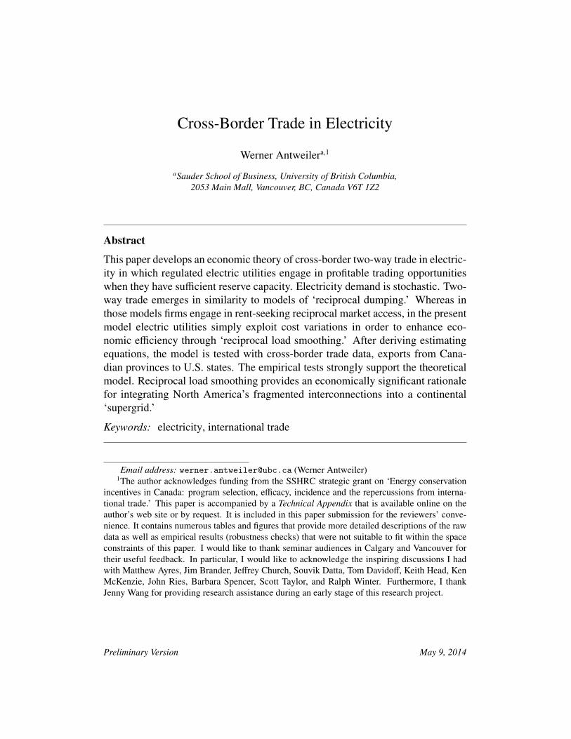
International trade in electricity is miniscule by the standard of overall tradein good services. In 2011, exports of electricity amounted to barely forty billionUS Dollars (and 662 TWh), only about 0.225% of the nearly eighteen trillion USDollars of worldwide trade. In that year only 87 nations reported positive exportsor imports. Yet trade in electricity has become vital for many countries, and asfigure 1 shows, in the last decade electricity trade has quadrupled.

Figure 1: Total World Exports of Electricity

Exp

orts

[US

$ bi

llons

]

05

1015202530354045

00 01 02 03 04 05 06 07 08 09 10 11 12

Source: UN Comtrade, HS 271600.

Unlike other commodities, elec-tricity cannot be stored; supply mustmeet demand instantaneously.2 As aresult, self-reliant jurisdictions needto maintain sufficient reserve gener-ation capacity to meet peaks in fluc-tuating demand. International tradeopens up opportunities to reduce ex-cessive reserve capacity as well asimport electricity from neighbouringcountries that have a comparative ad-

2A very small amount of electricity can be stored through hydroelectric reservoir pumping.Currently, there are no economically viable large-scale technological solutions for storing elec-tricity.

2

vantage in electricity generation due to favourable resource endowments. Tech-nologically, the main barrier to an increase in international trade in electricityhas been the problem of long-distance power transmission. High-voltage directcurrent (HVDC) transmission lines are more economical than alternating currenttransmission lines and can also be used for undersea links. Still, HVDC lossesamount to roughly 3.5% per thousand kilometer (about 6% per 1,000 miles), andconstructing new HVDC links remains very expensive. Among the most impor-tant HVDC links is the 1,362 km (846 miles) Pacific DC Intertie from northernOregon to Los Angeles. First completed in 1970, by 2004 it was upgraded to acapacity of 3.1 GW. Significant new construction of HVDC lines is currently un-der way (particularly in China and Brazil), although very little of the new capacitycrosses country borders.

Electricity generation in most jurisdictions is characterized by self-sufficiencymandates and a high level of government control. Because electricity distribu-tion (although not electricity generation) is a natural monopoly, governments of-ten exert control over electricity generation and distribution through governmentownership or through other forms of regulation (Everett, 2003). Retail prices forelectricity are set by utility commissions that largely amount to cost-plus mark-up rules. Experiments with privatization (such as in Britain) primarily focusedon electricity generation and electricity trading, with the implicit goal of pro-moting market entry of independent power producers (IPPs) that would competewith the established utilities (Rothwell and Gomez, 2003). The economics ofpower markets has attracted considerable attention due to the inherent complex-ities of electricity generation and transmission (Stoft, 2002; Harris, 2006). Be-cause of government-mandated self-sufficiency, trade in electricity across juris-dictional boundaries (both subnational and national) is mostly an afterthought,albeit a very profitable one. For trade economists, it is easy to identify excessiveself-sufficiency as autarkic inefficiency.

This paper approaches the issue of cross-border trade in electricity both the-oretically and empirically. To the best of my knowledge, mine is the first paperto tackle this issue in a rigorous trade-theoretical context by introducing a newmodel of two-way international trade.

The empirical reality of trade in electricity exhibits a pattern of two-way trade.Two-way trade is well understood within the context of product differentiation,where love-of-variety preferences lead to intra-industry trade where countries si-multaneously import and export similar (although not identical) goods. By com-parison, trade in a classical or neoclassical model is inter-industry—and thus one-way. While factor endowments clearly plays a role in determining comparative

3

advantage for electricity generation, the neoclassical model alone cannot accountfor the empirical reality of two-way trade. A new model is needed that can en-compass both one-way and two-way trade in electricity.

The theoretical section of this paper adapts the Brander (1981) and Branderand Krugman (1983) model of ‘reciprocal dumping’ to the context of efficiency-seeking trade in electricity. In addition to conventional comparative advantage, akey driver of trade in electricity is the stochastic variation in electricity demandacross jurisdiction coupled with the (often strong) convexity of electricity gener-ation cost. Under fairly general conditions, jurisdictions will engage in two-waytrade in electricity. Unlike Brander (1981), the reason for this two-way trade isnot strategic and rent-seeking because retail prices are regulated. Instead, two-waytrade is primarily efficiency-seeking through ‘reciprocal load smoothing.’

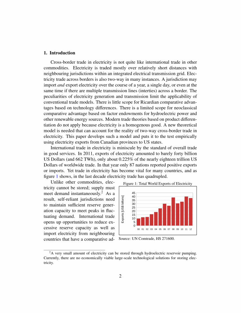
Understanding the rationale for electricity trade informs the quantification ofthe possible gains from trade. How (in)efficient is today’s trade regime? What isthe potential for additional gains from trade if the North American electric gridwas fully integrated? Indeed, a well-known source of inefficiency is the regionalseparation of electricity grids in North America, illustrated in figure 2.

Figure 2: North American Electricity Grid

Source: North American Electric Reliability Cor-poration

Transmission of bulk electricityin North America is managed bythe North American Electric Relia-bility Corporation (NERC) and inthe United States is regulated by theFederal Energy Regulatory Commis-sion (FERC). NERC’s standards andpolicies apply throughout the UnitedStates and Canada. There is infact no continent-wide grid. In-stead, there are several interconnec-tions (i.e., wide area synchronousgrids) that operate mostly separatefrom each other. The two most im-portant are the Western Interconnection and the Eastern Interconnection. Theother three interconnections serving Quebec, Alaska, and Texas are smaller insize. There are also nine NERC regional reliability councils that coordinate activ-ities in their corresponding regions. Transmitting power between interconnectionsis technically challenging, precluding trade among neighbouring jurisdictions andhampering long-distance east-west trading opportunities. To trade economists,North America’s power grid looks like free trade areas separated by tariff walls.

4

The empirical analysis in this paper makes use of export data from Cana-dian provinces to US states. The geographic west-east alignment of Canadianprovinces along the US border allows for trade with neighbouring provinces aswell as trade with many (not merely neighbouring) US states. Sufficiently disag-gregated data is available at the monthly level, allowing for the identification ofseasonal patterns in electricity trade. There is a limited number of cross-bordertrading pairs. Among the ten Canadian provinces and 49 landlocked US states(plus DC), there are 500 potential trading pairs. However, there are only 75 ac-tual trading pairs—or 15% of the potential. The extensive margin dominates thetrading patterns.

2. Empirical Patterns of Trade in Electricity

Table 1 shows average annual generation and demand of electricity in theten Canadian provinces and three territories. In most provinces, output and de-mand match closely. Most provincial utilities operate under a mandate of self-sufficiency. A few provinces export a significant amount of electricity to neigh-bouring provinces. For example, the province of Newfoundland and Labradorexports most of its electricity to neighbouring Quebec.3

Table 2 provides simple correlation statistics for electricity demand in the tenprovinces (aligned geographically from west to east). In some instances, demandcorrelation between neighbouring provinces is relatively high and exceeds 0.8.Interestingly, the correlation between two pairs of large provinces are modest:demand in Alberta and British Columbia is correlated at 0.37, and demand in On-tario and Quebec is correlated at 0.43. The point to take away is that correlationsare far less than perfect, and this opens up a source for gains from trade.

Table 3 extends the correlation analysis to the pairs of eight provinces and 32US states that are engaged in cross-border electricity trade. Actual trading part-ners are highlighted in boldface, while hypothetical trading partners are shown initalics. Many of the existing trade partners exhibit positively-correlated electric-ity demand. As the theoretical section will demonstrate later, lower and negativecorrelations are associated with a higher potential for trade. In the case of BritishColumbia, trade with California, Nevada, Arizona, New Mexico, and Texas is par-ticularly beneficial because of the negative correlations. As is easily seen, many

3The Churchill Falls hydroelectric dam in Labrador, with an installed capacity of 5,428Megawatt from 11 turbines, delivers electricity to the province of Quebec under a long-term powerpurchasing agreement that is a highly favourable to Quebec at today’s prices.

5

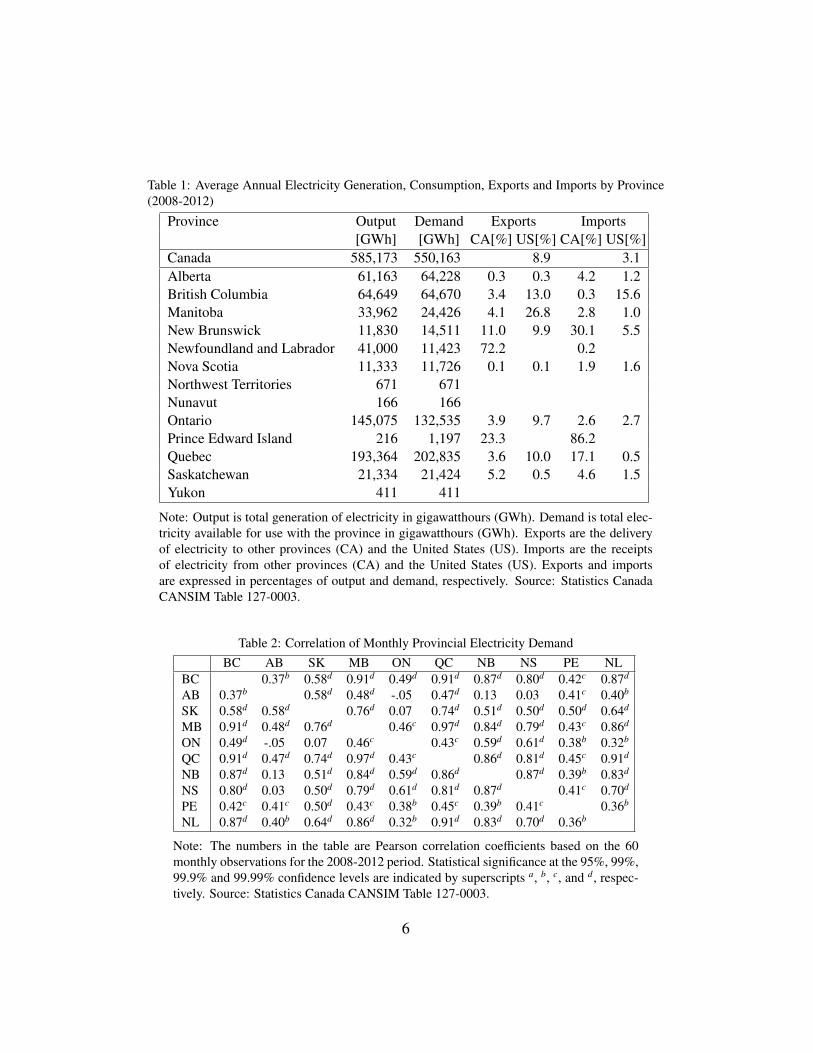
Table 1: Average Annual Electricity Generation, Consumption, Exports and Imports by Province(2008-2012)

Province Output Demand Exports Imports[GWh] [GWh] CA[%] US[%] CA[%] US[%]

Canada 585,173 550,163 8.9 3.1Alberta 61,163 64,228 0.3 0.3 4.2 1.2British Columbia 64,649 64,670 3.4 13.0 0.3 15.6Manitoba 33,962 24,426 4.1 26.8 2.8 1.0New Brunswick 11,830 14,511 11.0 9.9 30.1 5.5Newfoundland and Labrador 41,000 11,423 72.2 0.2Nova Scotia 11,333 11,726 0.1 0.1 1.9 1.6Northwest Territories 671 671Nunavut 166 166Ontario 145,075 132,535 3.9 9.7 2.6 2.7Prince Edward Island 216 1,197 23.3 86.2Quebec 193,364 202,835 3.6 10.0 17.1 0.5Saskatchewan 21,334 21,424 5.2 0.5 4.6 1.5Yukon 411 411

Note: Output is total generation of electricity in gigawatthours (GWh). Demand is total elec-tricity available for use with the province in gigawatthours (GWh). Exports are the deliveryof electricity to other provinces (CA) and the United States (US). Imports are the receiptsof electricity from other provinces (CA) and the United States (US). Exports and importsare expressed in percentages of output and demand, respectively. Source: Statistics CanadaCANSIM Table 127-0003.

Table 2: Correlation of Monthly Provincial Electricity DemandBC AB SK MB ON QC NB NS PE NL

BC 0.37b 0.58d 0.91d 0.49d 0.91d 0.87d 0.80d 0.42c 0.87d

AB 0.37b 0.58d 0.48d -.05 0.47d 0.13 0.03 0.41c 0.40b

SK 0.58d 0.58d 0.76d 0.07 0.74d 0.51d 0.50d 0.50d 0.64d

MB 0.91d 0.48d 0.76d 0.46c 0.97d 0.84d 0.79d 0.43c 0.86d

ON 0.49d -.05 0.07 0.46c 0.43c 0.59d 0.61d 0.38b 0.32b

QC 0.91d 0.47d 0.74d 0.97d 0.43c 0.86d 0.81d 0.45c 0.91d

NB 0.87d 0.13 0.51d 0.84d 0.59d 0.86d 0.87d 0.39b 0.83d

NS 0.80d 0.03 0.50d 0.79d 0.61d 0.81d 0.87d 0.41c 0.70d

PE 0.42c 0.41c 0.50d 0.43c 0.38b 0.45c 0.39b 0.41c 0.36b

NL 0.87d 0.40b 0.64d 0.86d 0.32b 0.91d 0.83d 0.70d 0.36b

Note: The numbers in the table are Pearson correlation coefficients based on the 60monthly observations for the 2008-2012 period. Statistical significance at the 95%, 99%,99.9% and 99.99% confidence levels are indicated by superscripts a, b, c, and d, respec-tively. Source: Statistics Canada CANSIM Table 127-0003.

6

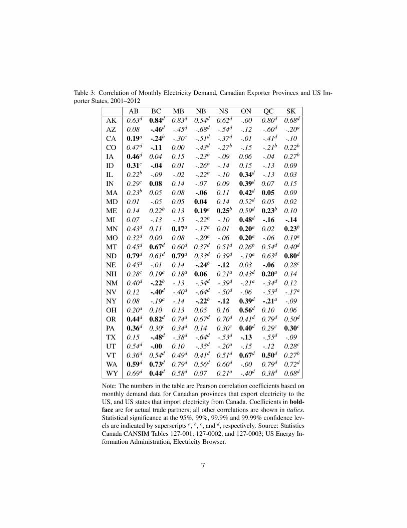
Table 3: Correlation of Monthly Electricity Demand, Canadian Exporter Provinces and US Im-porter States, 2001–2012

AB BC MB NB NS ON QC SKAK 0.63d 0.84d 0.83d 0.54d 0.62d -.00 0.80d 0.68d

AZ 0.08 -.46d -.45d -.68d -.54d -.12 -.60d -.20a

CA 0.19a -.24b -.30c -.51d -.37d -.01 -.41d -.10CO 0.47d -.11 0.00 -.43d -.27b -.15 -.21b 0.22b

IA 0.46d 0.04 0.15 -.23b -.09 0.06 -.04 0.27b

ID 0.31c -.04 0.01 -.26b -.14 0.15 -.13 0.09IL 0.22b -.09 -.02 -.22b -.10 0.34d -.13 0.03IN 0.29c 0.08 0.14 -.07 0.09 0.39d 0.07 0.15MA 0.23b 0.05 0.08 -.06 0.11 0.42d 0.05 0.09MD 0.01 -.05 0.05 0.04 0.14 0.52d 0.05 0.02ME 0.14 0.22b 0.13 0.19a 0.25b 0.59d 0.23b 0.10MI 0.07 -.13 -.15 -.22b -.10 0.48d -.16 -.14MN 0.43d 0.11 0.17a -.17a 0.01 0.20a 0.02 0.23b

MO 0.32d 0.00 0.08 -.20a -.06 0.20a -.06 0.19a

MT 0.45d 0.67d 0.60d 0.37d 0.51d 0.26b 0.54d 0.40d

ND 0.79d 0.61d 0.79d 0.33d 0.39d -.19a 0.63d 0.80d

NE 0.45d -.01 0.14 -.24b -.12 0.03 -.06 0.28c

NH 0.28c 0.19a 0.18a 0.06 0.21a 0.43d 0.20a 0.14NM 0.40d -.22b -.13 -.54d -.39d -.21a -.34d 0.12NV 0.12 -.40d -.40d -.64d -.50d -.06 -.55d -.17a

NY 0.08 -.19a -.14 -.22b -.12 0.39d -.21a -.09OH 0.20a 0.10 0.13 0.05 0.16 0.56d 0.10 0.06OR 0.44d 0.82d 0.74d 0.67d 0.70d 0.41d 0.79d 0.50d

PA 0.36d 0.30c 0.34d 0.14 0.30c 0.40d 0.29c 0.30c

TX 0.15 -.48d -.38d -.64d -.53d -.13 -.55d -.09UT 0.54d -.00 0.10 -.35d -.20a -.15 -.12 0.28c

VT 0.36d 0.54d 0.49d 0.41d 0.51d 0.67d 0.50d 0.27b

WA 0.59d 0.73d 0.79d 0.56d 0.60d -.00 0.79d 0.72d

WY 0.69d 0.44d 0.58d 0.07 0.21a -.40d 0.38d 0.68d

Note: The numbers in the table are Pearson correlation coefficients based onmonthly demand data for Canadian provinces that export electricity to theUS, and US states that import electricity from Canada. Coefficients in bold-face are for actual trade partners; all other correlations are shown in italics.Statistical significance at the 95%, 99%, 99.9% and 99.99% confidence lev-els are indicated by superscripts a, b, c, and d, respectively. Source: StatisticsCanada CANSIM Tables 127-001, 127-0002, and 127-0003; US Energy In-formation Administration, Electricity Browser.

7

pairs with high negative correlations are not engaging in trade—an indication ofunrealized trade potential.

Figure 3 illustrates the time dimension of electricity trade with the example ofBritish Columbia, which has one 500 kV intertie with the neighbouring provinceAlberta, and two 500 kV and two 230 kV interties with Washington state. Thisamounts to an export capacity of 3,150 MW to the United States and 1,200 MWto Alberta. For technical reasons, import capacities are slightly lower. As wasindicated in table 1, British Columbia’s total electricity trade is relatively balancedwith a significant amount of imports and exports. On closer inspection, exportsand imports exhibit seasonal patterns. Even over the period of a month, BritishColumbia tends to export and import electricity at the same time. This is in partexplained by the fact that there are multiple interties. British Columbia’s availablegeneration capacity depends on water levels in the reservoirs of its hydroelectricdams. Thus there is surplus electricity in high-water years. The years 2011 and2012 exhibited large net exports during the summer months. Electricity trade withAlberta, shown in figure 4, contributes relatively little to the overall trade becauseof the smaller capacity of the interties. The trading pattern is clearly dominatedby exports, indicating that British Columbia has a strong comparative advantagein electricity generation with respect to neighbouring Alberta.

Figure 5 shows the volume of bilateral Canada-US trade over the last decade.Canada runs an electricity surplus with the United States, with US imports ofCanadian electricity about twice the volume of US exports to Canada. Pricescan fluctuate significantly, as is illustrated in figure 6. Electricity can trade foras little as $25 per MWh, and as much as $70 per MWh. Canadian electricitycommands an export price premium. Over the twelve-year period in the diagram,Canadian electricity exports to the US cost about 20% more than US electricityexports to Canada (15% volume-weighted, 23% unweighted) despite the apparentcomparative advantage of Canada in electricity production suggested in figure 5.

One of the peculiarities of international trade in electricity is that the price doesnot necessarily reflect resource abundance in a conventional Heckscher-Ohlinsense. The price of traded electricity depends as much on long-term compara-tive advantage as it does on short-term shortages. The result is that electricity—ahomogenous commodity—can be priced rather differently depending on whichway the electricity flows through an intertie. The ‘law of one price’ does not ap-ply. Pricing may even reach absurd levels. During the California electricity crisisin 2000/2001, British Columbia exported electricity to California at peak prices ofaround $800/MWh (see also figures TA-1 and TA-2 in the Technical Appendix).And in March 2013, Ontario exported electricity to New York and Michigan at

8

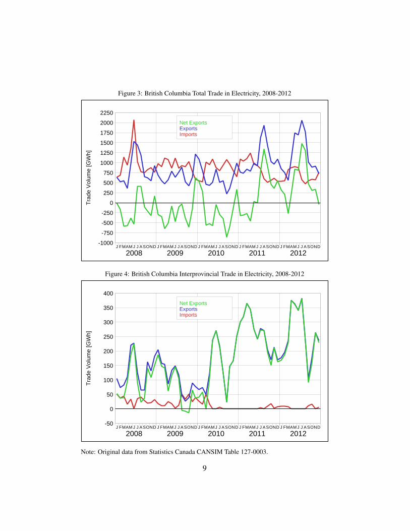
Figure 3: British Columbia Total Trade in Electricity, 2008-2012T

rade

Vol

ume

[GW

h]

-1000

-750

-500

-250

0

250

500

750

1000

1250

1500

1750

2000

2250

J FMAM J

2008J A SOND J FMAM J

2009J A SOND J FMAM J

2010J A SOND J FMAM J

2011J A SOND J FMAM J

2012J A SOND

ImportsExportsNet Exports

Figure 4: British Columbia Interprovincial Trade in Electricity, 2008-2012

Tra

de V

olum

e [G

Wh]

-50

0

50

100

150

200

250

300

350

400

J FMAM J

2008J A SOND J FMAM J

2009J A SOND J FMAM J

2010J A SOND J FMAM J

2011J A SOND J FMAM J

2012J A SOND

ImportsExportsNet Exports

Note: Original data from Statistics Canada CANSIM Table 127-0003.

9

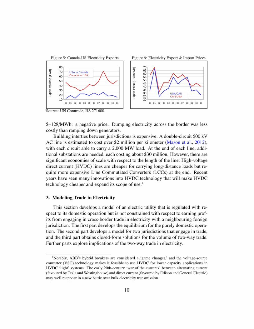
Figure 5: Canada-US Electricity Exports

Exp

ort V

olum

e [T

Wh]

10

20

30

40

50

60

70

80

00 01 02 03 04 05 06 07 08 09 10 11

Canada to USAUSA to Canada

Figure 6: Electricity Export & Import Prices

Exp

ort P

rice

[US

$/M

Wh]

2025303540455055606570

00 01 02 03 04 05 06 07 08 09 10 11

CAN/USAUSA/CAN

Source: UN Comtrade, HS 271600

$–128/MWh: a negative price. Dumping electricity across the border was lesscostly than ramping down generators.

Building interties between jurisdictions is expensive. A double-circuit 500 kVAC line is estimated to cost over $2 million per kilometer (Mason et al., 2012),with each circuit able to carry a 2,000 MW load. At the end of each line, addi-tional substations are needed, each costing about $30 million. However, there aresignificant economies of scale with respect to the length of the line. High-voltagedirect current (HVDC) lines are cheaper for carrying long-distance loads but re-quire more expensive Line Commutated Converters (LCCs) at the end. Recentyears have seen many innovations into HVDC technology that will make HVDCtechnology cheaper and expand its scope of use.4

3. Modeling Trade in Electricity

This section develops a model of an electric utility that is regulated with re-spect to its domestic operation but is not constrained with respect to earning prof-its from engaging in cross-border trade in electricity with a neighbouring foreignjurisdiction. The first part develops the equilibrium for the purely domestic opera-tion. The second part develops a model for two jurisdictions that engage in trade,and the third part obtains closed-form solutions for the volume of two-way trade.Further parts explore implications of the two-way trade in electricity.

4Notably, ABB’s hybrid breakers are considered a ‘game changer,’ and the voltage-sourceconverter (VSC) technology makes it feasible to use HVDC for lower capacity applications inHVDC ‘light’ systems. The early 20th-century ‘war of the currents’ between alternating current(favoured by Tesla and Westinghouse) and direct current (favoured by Edison and General Electric)may well reappear in a new battle over bulk electricity transmission.

10

The model of ‘reciprocal load smoothing’ developed here introduces a noveltype of comparative advantage. However, I will continue to use the term ‘compar-ative advantage’ to refer to the fixed long-term comparative advantage from factorendowments in the Heckscher-Ohlin sense, and contrast this with the variableshort-term comparative advantage from load asymmetries between jurisdictions.

3.1. One JurisdictionThe most significant starting point for modeling an electric utility is its cost

function. Power generation is characterized by a least-cost-first approach to de-ploying power plants. Base load utilizes power plants with low marginal cost suchas hydroelectric dams, or nuclear power plants whose output is difficult to rampup or down. Peak load utilizes power plants with short ramping times but highfuel costs. A sufficiently general cost function for electricity generation is

c(q(t)) = c0 + c1q(t) +12

c2q(t)2 (1)

Figure 7: Load and Cost Variation

Load

MC

c1

qmin qmaxq0 q1q2

1

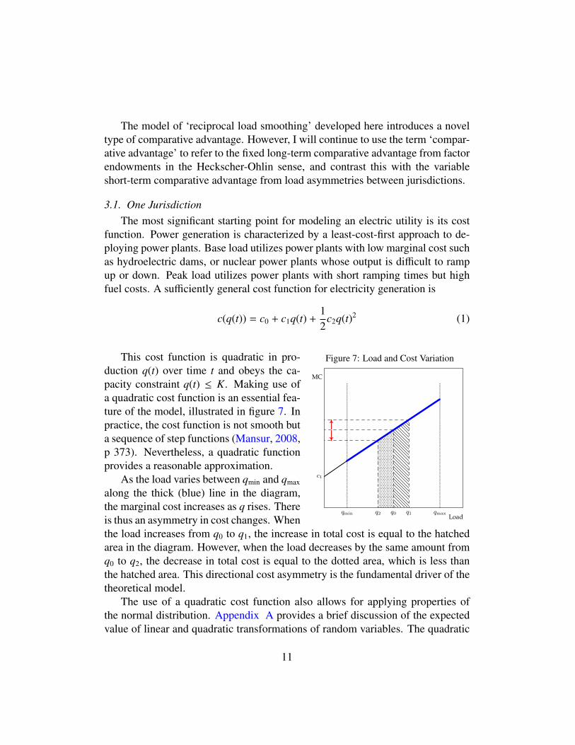
This cost function is quadratic in pro-duction q(t) over time t and obeys the ca-pacity constraint q(t) ≤ K. Making use ofa quadratic cost function is an essential fea-ture of the model, illustrated in figure 7. Inpractice, the cost function is not smooth buta sequence of step functions (Mansur, 2008,p 373). Nevertheless, a quadratic functionprovides a reasonable approximation.

As the load varies between qmin and qmax

along the thick (blue) line in the diagram,the marginal cost increases as q rises. Thereis thus an asymmetry in cost changes. Whenthe load increases from q0 to q1, the increase in total cost is equal to the hatchedarea in the diagram. However, when the load decreases by the same amount fromq0 to q2, the decrease in total cost is equal to the dotted area, which is less thanthe hatched area. This directional cost asymmetry is the fundamental driver of thetheoretical model.

The use of a quadratic cost function also allows for applying properties ofthe normal distribution. Appendix A provides a brief discussion of the expectedvalue of linear and quadratic transformations of random variables. The quadratic

11

cost function is particularly suited to exploiting this concept to derive analyticallytractable solutions to the utility’s profit maximization problem. Nevertheless, keyresults of this paper—in particular for the problem of electricity trade betweentwo jurisdictions—can also be derived with alternative cost functions. AppendixD discusses a logarithmic cost function that is based on capacity utilization (q/K).

For delivery of electricity within a single jurisdiction, transmission losses areassumed as part of the cost function. When considering cross-jurisdictional deliv-ery of electricity, transmissions costs will be taken into account explicitly.

Demand for electricity is determined long-term and short-term. Average de-mand q over a sufficiently long reference period (assumed to be a year) is governedby a linear demand function

q = a − bp (2)

where the utility price p is set by a utility commission as described below. Manyutilities still opt for a relatively “flat” pricing system, in the simplest case witha single price. Peak-load pricing, although economically optimal, is only slowlygaining ground.5 Within the reference period, short-term demand is determinedstochastically as

q(t) ∼ N(q, s2) (3)

so that over the integration time period [0,T ], or equivalently over the probabilitydistribution of demand f (q) during the time period T , total supply is∫ T

0q(t)dt = T

∫f (q) dq = qT (4)

Having defined revenues and costs, the utility company’s profits over a fiscal year

5For example, the province of Ontario now uses time-of-day residential pricing (on-peak, mid-peak, and off-peak during weekdays, and off-peak during weekends) as well as seasonal pricing(mid-peak and on-peak periods are reversed in summer and winter). Peak-load pricing in Ontarioleads to significantly different retail rates for electricity. As of May 1, 2013, the prices for off-peak,mid-peak, and on-peak were 6.7, 10.4 and 12.4 cents per kWh, respectively. By comparison, theprovince of British Columbia uses a two-step system that amounts to de-facto seasonal pricing.As of April 1, 2013, residential rates are set at 6.90 cents per kWh for the first 675 kWh permonth, and at 10.34 cents per kWh for electric power above the threshold. As electricity demandin British Columbia peaks in the winter due to heating needs, consumers face a higher marginalprice in winter than in summer.

12

are given by

π =

∫ [pq(t) − c(q(t))

]dt (5)

Because of the natural monopoly in electricity distribution, a utility’s profits areusually constrained in some form (see Bernard and Roland, 1997). A commonform is the fixed mark-up where the retail price p is set in such a way that theutility realizes a fixed percentage mark-up η over the reference period. For agiven value of the policy parameter η,

p = (1 + η)

∫c(t)dt∫q(t)dt

= (1 + η)[c0 + c2s2

q+ c1 + c2q

](6)

The utility’s retail price for electricity is a mark-up on marginal cost at averageload (c1+ c2q) plus a component for absorbing the fixed cost and the variability ofdemand that is caused by the asymmetry in costs that was illustrated in figure 7.The retail price increases with the variance s2. More volatile loads are associatedwith higher electricity retail prices because of a stronger exposure to the costasymmetry. Equations (2) and (6) together characterize the long-term equilibrium.For a given η, the two equations identify the equilibrium outcome {p, q}.6

3.2. Two JurisdictionsLet there be two jurisdictions, home (h) and foreign (f). Where a distinction

between home and foreign needs to be made, corresponding superscripts are used.At any given time, the home jurisdiction can export a flow of electric power

x(t) to the foreign jurisdiction. A negative x(t) constitutes an import of electricpower. Transporting electricity across jurisdictional boundaries incurs a transmis-sion cost g|x| that is proportional to the amount (absolute value |x|) of electricalpower transmitted. The parameter g is a function of the distance D between thejurisdictions.7 It is assumed that the transmission cost is split equally between

6If the utility would use peak-load pricing instead of flat pricing, the demand fluctuations wouldbe dampened by consumers’ adjustment to the changing prices. This will change the time path forthe actual loads q(t) and reduce its variance s2.

7It may be appealing to model transmission costs in terms of actual electricity losses—reminiscent of ‘iceberg transportation costs’ in the international trade literature. However, thisapproach increases algebraic complexity significantly with very little gain in economic insights.Modeling transmission costs as a linear function of exports or imports is a suitable approximationof reality. An alternate logarithmic cost function is explored in Appendix D where the transmis-

13

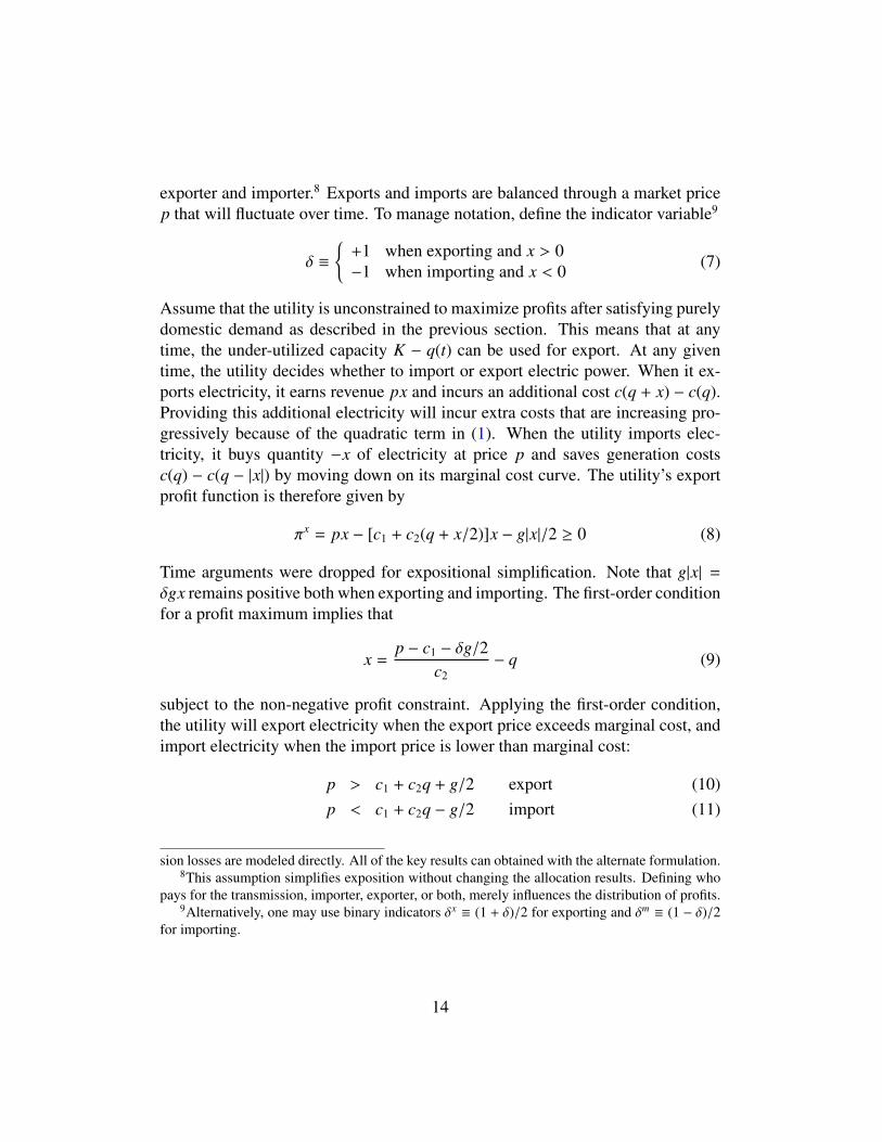
exporter and importer.8 Exports and imports are balanced through a market pricep that will fluctuate over time. To manage notation, define the indicator variable9

δ ≡

{+1 when exporting and x > 0−1 when importing and x < 0 (7)

Assume that the utility is unconstrained to maximize profits after satisfying purelydomestic demand as described in the previous section. This means that at anytime, the under-utilized capacity K − q(t) can be used for export. At any giventime, the utility decides whether to import or export electric power. When it ex-ports electricity, it earns revenue px and incurs an additional cost c(q + x) − c(q).Providing this additional electricity will incur extra costs that are increasing pro-gressively because of the quadratic term in (1). When the utility imports elec-tricity, it buys quantity −x of electricity at price p and saves generation costsc(q) − c(q − |x|) by moving down on its marginal cost curve. The utility’s exportprofit function is therefore given by

πx = px − [c1 + c2(q + x/2)]x − g|x|/2 ≥ 0 (8)

Time arguments were dropped for expositional simplification. Note that g|x| =δgx remains positive both when exporting and importing. The first-order conditionfor a profit maximum implies that

x =p − c1 − δg/2

c2− q (9)

subject to the non-negative profit constraint. Applying the first-order condition,the utility will export electricity when the export price exceeds marginal cost, andimport electricity when the import price is lower than marginal cost:

p > c1 + c2q + g/2 export (10)p < c1 + c2q − g/2 import (11)

sion losses are modeled directly. All of the key results can obtained with the alternate formulation.8This assumption simplifies exposition without changing the allocation results. Defining who

pays for the transmission, importer, exporter, or both, merely influences the distribution of profits.9Alternatively, one may use binary indicators δx ≡ (1 + δ)/2 for exporting and δm ≡ (1 − δ)/2

for importing.

14

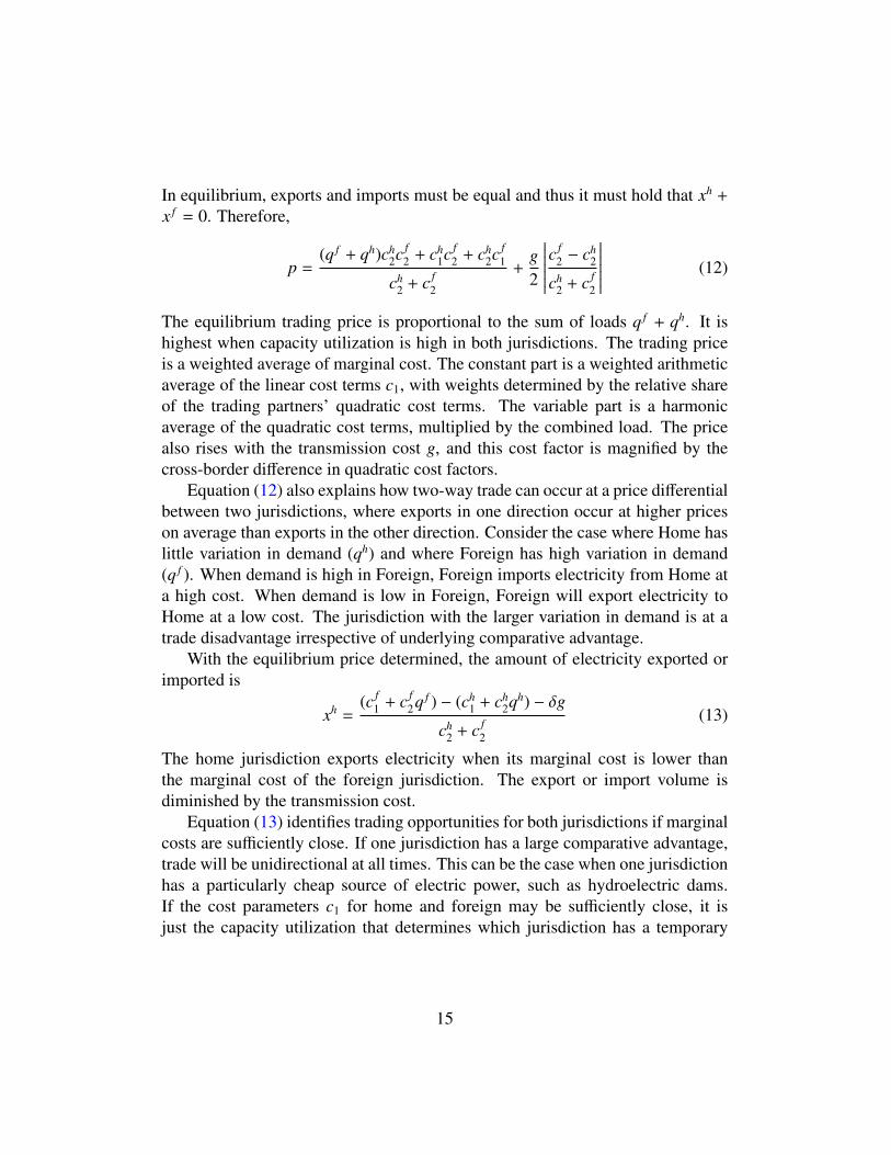
In equilibrium, exports and imports must be equal and thus it must hold that xh +

x f = 0. Therefore,

p =(q f + qh)ch

2c f2 + ch

1c f2 + ch

2c f1

ch2 + c f

2

+g2

∣∣∣∣∣∣∣cf2 − ch

2

ch2 + c f

2

∣∣∣∣∣∣∣ (12)

The equilibrium trading price is proportional to the sum of loads q f + qh. It ishighest when capacity utilization is high in both jurisdictions. The trading priceis a weighted average of marginal cost. The constant part is a weighted arithmeticaverage of the linear cost terms c1, with weights determined by the relative shareof the trading partners’ quadratic cost terms. The variable part is a harmonicaverage of the quadratic cost terms, multiplied by the combined load. The pricealso rises with the transmission cost g, and this cost factor is magnified by thecross-border difference in quadratic cost factors.

Equation (12) also explains how two-way trade can occur at a price differentialbetween two jurisdictions, where exports in one direction occur at higher priceson average than exports in the other direction. Consider the case where Home haslittle variation in demand (qh) and where Foreign has high variation in demand(q f ). When demand is high in Foreign, Foreign imports electricity from Home ata high cost. When demand is low in Foreign, Foreign will export electricity toHome at a low cost. The jurisdiction with the larger variation in demand is at atrade disadvantage irrespective of underlying comparative advantage.

With the equilibrium price determined, the amount of electricity exported orimported is

xh =(c f

1 + c f2q f ) − (ch

1 + ch2qh) − δg

ch2 + c f

2

(13)

The home jurisdiction exports electricity when its marginal cost is lower thanthe marginal cost of the foreign jurisdiction. The export or import volume isdiminished by the transmission cost.

Equation (13) identifies trading opportunities for both jurisdictions if marginalcosts are sufficiently close. If one jurisdiction has a large comparative advantage,trade will be unidirectional at all times. This can be the case when one jurisdictionhas a particularly cheap source of electric power, such as hydroelectric dams.If the cost parameters c1 for home and foreign may be sufficiently close, it isjust the capacity utilization that determines which jurisdiction has a temporary

15

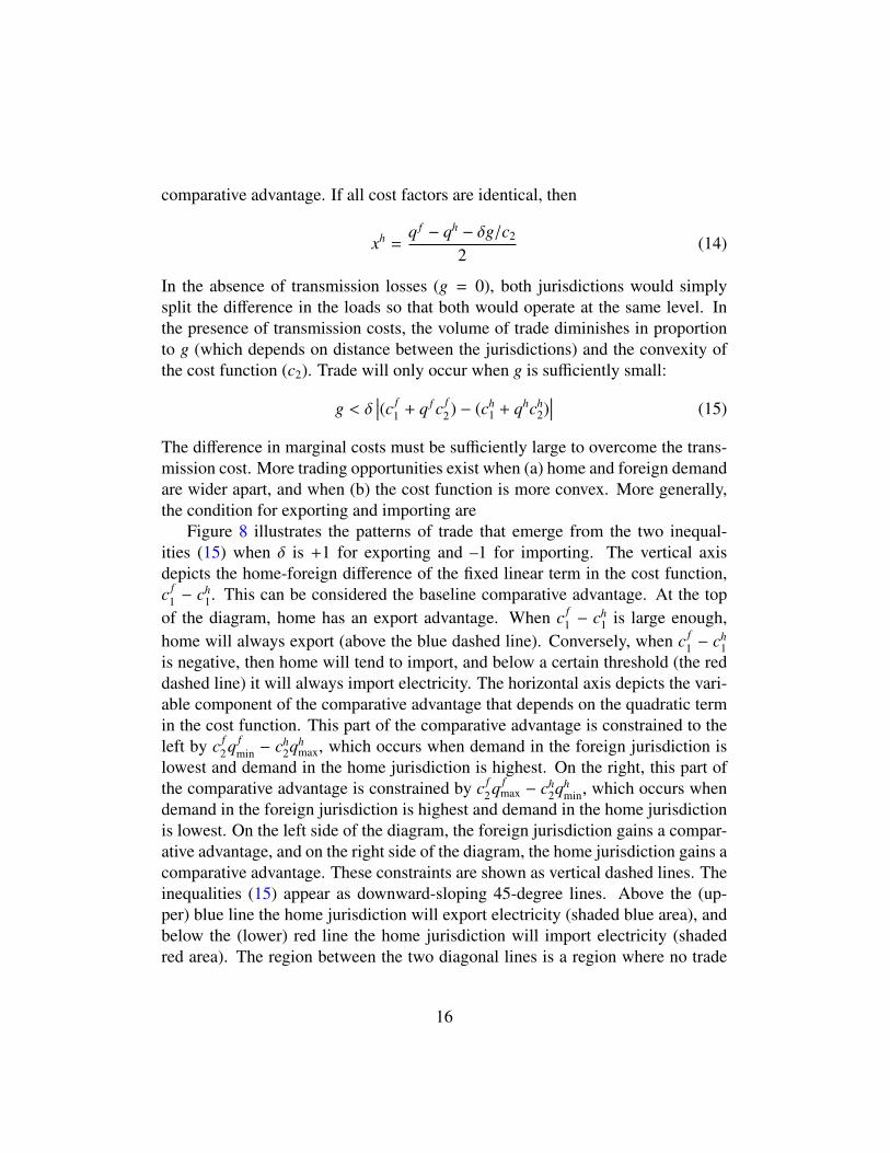
comparative advantage. If all cost factors are identical, then

xh =q f − qh − δg/c2

2(14)

In the absence of transmission losses (g = 0), both jurisdictions would simplysplit the difference in the loads so that both would operate at the same level. Inthe presence of transmission costs, the volume of trade diminishes in proportionto g (which depends on distance between the jurisdictions) and the convexity ofthe cost function (c2). Trade will only occur when g is sufficiently small:

g < δ∣∣∣(c f

1 + q f c f2) − (ch

1 + qhch2)∣∣∣ (15)

The difference in marginal costs must be sufficiently large to overcome the trans-mission cost. More trading opportunities exist when (a) home and foreign demandare wider apart, and when (b) the cost function is more convex. More generally,the condition for exporting and importing are

Figure 8 illustrates the patterns of trade that emerge from the two inequal-ities (15) when δ is +1 for exporting and –1 for importing. The vertical axisdepicts the home-foreign difference of the fixed linear term in the cost function,c f

1 − ch1. This can be considered the baseline comparative advantage. At the top

of the diagram, home has an export advantage. When c f1 − ch

1 is large enough,home will always export (above the blue dashed line). Conversely, when c f

1 − ch1

is negative, then home will tend to import, and below a certain threshold (the reddashed line) it will always import electricity. The horizontal axis depicts the vari-able component of the comparative advantage that depends on the quadratic termin the cost function. This part of the comparative advantage is constrained to theleft by c f

2q fmin − ch

2qhmax, which occurs when demand in the foreign jurisdiction is

lowest and demand in the home jurisdiction is highest. On the right, this part ofthe comparative advantage is constrained by c f

2q fmax − ch

2qhmin, which occurs when

demand in the foreign jurisdiction is highest and demand in the home jurisdictionis lowest. On the left side of the diagram, the foreign jurisdiction gains a compar-ative advantage, and on the right side of the diagram, the home jurisdiction gains acomparative advantage. These constraints are shown as vertical dashed lines. Theinequalities (15) appear as downward-sloping 45-degree lines. Above the (up-per) blue line the home jurisdiction will export electricity (shaded blue area), andbelow the (lower) red line the home jurisdiction will import electricity (shadedred area). The region between the two diagonal lines is a region where no trade

16

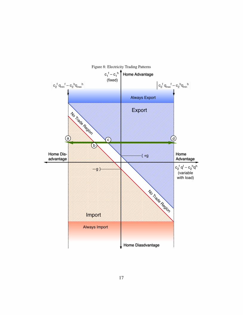
Figure 8: Electricity Trading Patterns

Home Advantage Home Advantage

Home Diasdvantage Home Diasdvantage

HomeAdvantage

HomeAdvantage

Home Dis-advantage

Home Dis-advantage

c1f – c1h

(fixed)

c2f qf – c2hqh

c2f qmaxf – c2hqmin

hc2f qmaxf – c2hqmin

hc2f qminf – c2hqmax

hc2f qminf – c2hqmax

h

No Trade Region

No Trade Region

Export

Always Export

Always Import

Import

(variablewith load)

a dcb

—g }

{ +g

17

takes place because the gains from trade do not compensate for the transmissioncosts. In the diagram the minimum c f

2q fmin − ch

2qhmax and maximum c f

2q fmax − ch

2qhmin

have been centered around zero for illustration purposes. Depending on the exactparameters, these expressions could be asymmetric, including all positive or allnegative.

A particular pair of jurisdictions will operate on a horizontal line, for examplethe thick green line in the diagram. This particular case illustrates a situationwhere the home jurisdiction has a slight fixed-part advantage because c f

1 > ch1.

As demand fluctuates, the variable-part advantage moves along the horizontal linebetween the minimum at point (a) and maximum at point (d). If demand in theforeign jurisdiction is high, and this jurisdiction experiences high marginal costsof production, the home jurisdiction gains an increasing export advantage movingfrom point (c) right to point (d). On the other hand, as demand at home is highand demand abroad is low, the home jurisdiction will shift further to the left,eventually cross point (b) and start importing electricity. As demand at homegrows further, the home jurisdiction will experience increasing disadvantages asit moves towards point (a). Between points (b) and (c), engaging in electricitytrade will not be profitable because of the transmission costs.

3.3. The Volume of Two-Way TradeThe discussion of the previous section demonstrates that electricity trade can

be unidirectional or bidirectional over a sufficiently time period. While at anygiven point in time (with a single intertie) electricity can only flow one way, overthe course of a day, month, or year electricity can flow either direction as demandchanges in both jurisdictions. This is particularly the case if demand across bothjurisdictions is not perfectly correlated, for example because of different seasonalpatterns. For simplicity of exposition, assume that home and foreign demand aredistributed bivariate normal with correlation coefficient ρ so that[

qh(t)q f (t)

]= N

([qh

q f

],

[(sh)2 ρshs f

ρshs f (s f )2

])(16)

Making use of the affine transformation formula for multivariate normal dis-tributions, explained in Appendix B, one obtains:

18

u ≡ E{xh} =(c f

1 + c2f q

f ) − (ch1 + ch

2qh) − δg

ch2 + c f

2

(17)

v2 ≡ V{xh} =(ch

2sh)2 − 2ch2c f

2 shs fρ + (c f2 s f )2

(ch2 + c f

2)2(18)

Evaluating the truncated normal distribution as described in Appendix C pro-vides expressions for the total volume of Home’s exports Xh and total volume ofHome’s imports Mh over the reference period. Let ux denote the version of (17)for exporting when δ = +1, and let um denote the version of (17) for importingwhen δ = −1. Integrating over the reference period yields

Xh ≡

∫xh>0

xh(t) dt =[ux + v

φ(ux/v)Φ(ux/v)

]T (19)

Analogously, Home’s volume of imports is given by

Mh ≡

∫xh<0−xh(t) dt =

[−um + v

φ(um/v)1 − Φ(um/v)

]T (20)

The variance expression v2 is of crucial importance for determining the volume ofexports and imports: there is a positive sign in front of v in the case of exportingand importing. By definition, φ(·) > 0 and Φ(·) ∈]0, 1[, and thus v always has apositive influence on Xh and Mh. The larger the variance v2, the more bilateraltrade. The correlation coefficient ρ plays an important role determining the vari-ance v2. The derivative of v2 with respect to ρ is clearly negative, which impliesthat higher correlation diminishes trade. This is a very intuitive—and essential—feature. If demand is strongly correlated between jurisdictions, they will both ex-perience high demand and low demand simultaneously, and this leaves little roomfor additional trade. However, when demand in both jurisdictions is correlatednegatively, they can benefit from increased trade.

The derivation above gives rise to an expression for the trade intensity, (Xh +

Mh)/Qh, where Qh ≡∫

q(t)dt is total demand. For expositional simplicity, it isexpedient to ignore the transmission costs g so that ux = um. Then

Xh + Mh

Qh =vqh

φ(u/v)Φ(u/v)Φ(−u/v)

(21)

19

It is interesting to investigate the case where both jurisdictions are identical (samecost coefficients, qh = q f , and sh = s f ). Then u/v = 0 and φ(0)/Φ(0) =

√2/π.

Hence:Xh + Mh

Qh

∣∣∣∣∣∣h= f

=sq

√4π

(1 − ρ) (22)

The trade intensity increases along with the coefficient of variation τ ≡ s/q and adecreasing coefficient of demand correlation between the two jurisdictions ρ.

Yet another simplification is useful to look at. Consider the case where thetwo jurisdictions are different in size by a factor of ζ so that q f = (1 + ζ)qh ands f = (1+ ζ)sh. Both jurisdictions exhibit the same coefficient of variation τ ≡ s/q.Further assume that their demand is perfectly correlated (ρ = 1). Then

Xh + Mh

Qh

∣∣∣∣∣∣ρ=1, f /h=1+ζ

=ζ

2τφ(1/τ)

Φ(1/τ)(1 − Φ(1/τ))≈ζ

2(23)

The approximation improves when τ → 0 and holds reasonably well for smallvalues of τ (e.g., for τ = 1/4 it is 0.5282ζ). When the size difference between thejurisdictions decreases towards zero (ζ → 0), the trading opportunity will vanishcompletely because of the perfect demand correlation (ρ = 1).

The case where jurisdictions only differ in size creates an opportunity for tradethat is proportional to the size difference ζ. The economic intuition behind thisresult is that the marginal cost accelerator c2 works differently in the two jurisdic-tions. In the larger jurisdiction, demand variations move up and down the marginalcost curve “faster” than in the smaller jurisdiction. The larger jurisdiction thus ex-periences larger cost variations than the smaller jurisdiction.

3.4. Decomposing One-Way and Two-Way TradeThe model introduced in this paper allows both for one-way trade (driven by

comparative advantage in electricity generation) and two-way trade (driven by thebenefits of reciprocal load smoothing). Available trade data aggregates both typesof trade into one figure. Can they be decomposed?

A conventional measure for measuring the extent of two-way trade is theGrubel and Lloyd (1971) index

GLt = 1 −|Xt − Mt|

Xt + Mt(24)

This means that total trade X +M can be decomposed into one-way trade |X −M|

20

and two-way trade (X + M) − |X − M|. Thus the GL index captures the share oftwo-trade trade. Using the expressions for exports (19) and imports (20), ignoringtransportation costs g, and defining the ratio θ ≡ |u|/v as the normalized tradevolume, it can be shown that

GL(θ) = 2Φ(θ)[1 − θ

1 − Φ(θ)φ(θ)

](25)

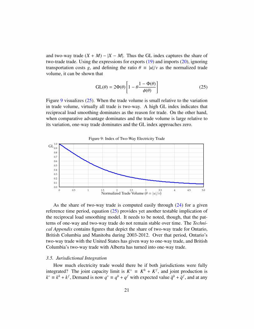
Figure 9 visualizes (25). When the trade volume is small relative to the variationin trade volume, virtually all trade is two-way. A high GL index indicates thatreciprocal load smoothing dominates as the reason for trade. On the other hand,when comparative advantage dominates and the trade volume is large relative toits variation, one-way trade dominates and the GL index approaches zero.

Figure 9: Index of Two-Way Electricity Trade

0 1 2 3 40.5 1.5 2.5 3.5 4.5

0.1

0.2

0.3

0.4

0.5

0.6

0.7

0.8

0.9

1.0

0.05.0

GL

Normalized Trade Volume (θ ≡ |u|/v)

1As the share of two-way trade is computed easily through (24) for a givenreference time period, equation (25) provides yet another testable implication ofthe reciprocal load smoothing model. It needs to be noted, though, that the pat-terns of one-way and two-way trade do not remain stable over time. The Techni-cal Appendix contains figures that depict the share of two-way trade for Ontario,British Columbia and Manitoba during 2003-2012. Over that period, Ontario’stwo-way trade with the United States has given way to one-way trade, and BritishColumbia’s two-way trade with Alberta has turned into one-way trade.

3.5. Jurisdictional IntegrationHow much electricity trade would there be if both jurisdictions were fully

integrated? The joint capacity limit is K◦ ≡ Kh + K f , and joint production isk◦ ≡ kh + k f , Demand is now q◦ ≡ qh + q f with expected value qh + q f , and at any

21

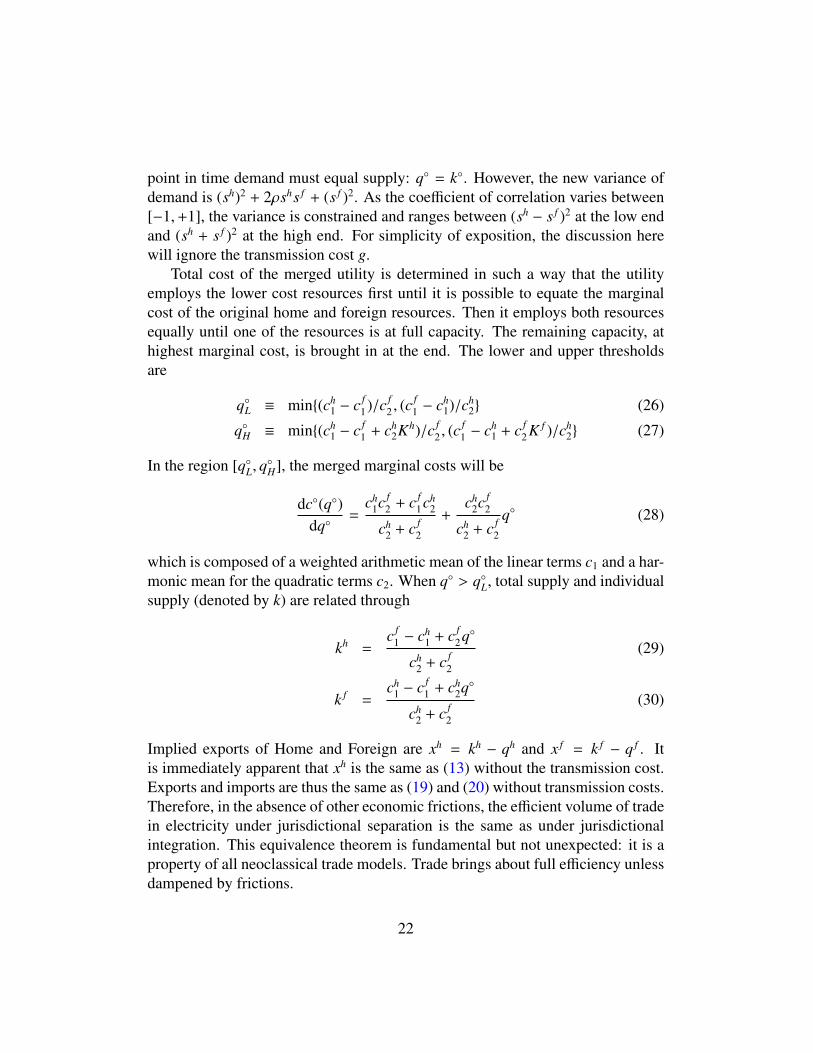
point in time demand must equal supply: q◦ = k◦. However, the new variance ofdemand is (sh)2 + 2ρshs f + (s f )2. As the coefficient of correlation varies between[−1,+1], the variance is constrained and ranges between (sh − s f )2 at the low endand (sh + s f )2 at the high end. For simplicity of exposition, the discussion herewill ignore the transmission cost g.

Total cost of the merged utility is determined in such a way that the utilityemploys the lower cost resources first until it is possible to equate the marginalcost of the original home and foreign resources. Then it employs both resourcesequally until one of the resources is at full capacity. The remaining capacity, athighest marginal cost, is brought in at the end. The lower and upper thresholdsare

q◦L ≡ min{(ch1 − c f

1)/c f2 , (c

f1 − ch

1)/ch2} (26)

q◦H ≡ min{(ch1 − c f

1 + ch2Kh)/c f

2 , (cf1 − ch

1 + c f2 K f )/ch

2} (27)

In the region [q◦L, q◦H], the merged marginal costs will be

dc◦(q◦)dq◦

=ch

1c f2 + c f

1ch2

ch2 + c f

2

+ch

2c f2

ch2 + c f

2

q◦ (28)

which is composed of a weighted arithmetic mean of the linear terms c1 and a har-monic mean for the quadratic terms c2. When q◦ > q◦L, total supply and individualsupply (denoted by k) are related through

kh =c f

1 − ch1 + c f

2q◦

ch2 + c f

2

(29)

k f =ch

1 − c f1 + ch

2q◦

ch2 + c f

2

(30)

Implied exports of Home and Foreign are xh = kh − qh and x f = k f − q f . Itis immediately apparent that xh is the same as (13) without the transmission cost.Exports and imports are thus the same as (19) and (20) without transmission costs.Therefore, in the absence of other economic frictions, the efficient volume of tradein electricity under jurisdictional separation is the same as under jurisdictionalintegration. This equivalence theorem is fundamental but not unexpected: it is aproperty of all neoclassical trade models. Trade brings about full efficiency unlessdampened by frictions.

22

In practice, jurisdictional integration has two advantages over jurisdictionalseparation. First, integration removes the potential conflict over building sufficientintertie capacity. Integration eliminates the negotiation and contracting issues thatmay arise otherwise. Second, integration also leads to a new price p, which—aswas shown earlier—is influenced by the variance of the distribution of q(t). Ifdemand in both jurisdictions is less than perfectly correlated, integration will leadto a reduction of the joint variance s2; it will be lower than (sh)2 + (s f )2. Thismeans that the joint price p can be lower than the original ph or p f (unless theoriginal price gap was very large). This ‘integration bonus’ is a true efficiencygain.

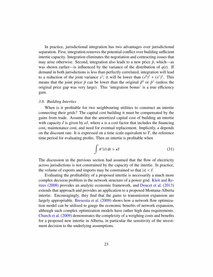
3.6. Building IntertiesWhen is it profitable for two neighbouring utilities to construct an intertie

connecting their grids? The capital cost building it must be compensated by thegains from trade. Assume that the amortized capital cost of building an intertiewith capacity I is given by κI, where κ is a cost factor that includes the financingcost, maintenance cost, and need for eventual replacement. Implicitly, κ dependson the discount rate. It is expressed on a time scale equivalent to T , the referencetime period for evaluating profits. Then an intertie is profitable when∫

πx(t) dt > κI (31)

The discussion in the previous section had assumed that the flow of electricityacross jurisdictions is not constrained by the capacity of the intertie. In practice,the volume of exports and imports may be constrained so that |x| < I.

Evaluating the profitability of a proposed intertie is necessarily a much morecomplex decision problem in the network structure of a power grid. Kleit and Re-itzes (2008) provides an analytic economic framework, and Doucet et al. (2013)extends that approach and provides an application to a proposed Montana-Albertaintertie. Encouragingly, they find that the gains to transmission expansion arelargely appropriable. Bresestia et al. (2009) shows how a network flow optimiza-tion model can be utilized to gauge the economic benefits of network expansion,although such complex optimization models have rather high data requirements.Church et al. (2009) demonstrates the complexity of a weighing costs and benefitsfor a proposed new intertie in Alberta, in particular the sensitivity of the invest-ment decision to the underlying assumptions.

23

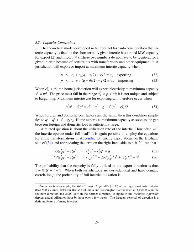
3.7. Capacity ConstraintsThe theoretical model developed so far does not take into consideration that in-

tertie capacity is fixed in the short term. A given intertie has a rated MW capacityfor export (x) and import (m). These two numbers do not have to be identical for agiven intertie because of constraints with transformers and other equipment.10 Ajurisdiction will export or import at maximum intertie capacity when

p > c1 + c2(q + x/2) + g/2 ≡ cx exporting (32)p < c1 + c2(q − m/2) − g/2 ≡ cm importing (33)

When c fm < ch

x, the home jurisdiction will export electricity at maximum capacityxh = m f . The price must fall in the range c f

m < p < chx; it is not unique and subject

to bargaining. Maximum intertie use for exporting will therefore occur when

c f2q f − ch

2qh > ch1 − c f

1 + g + xh(c f2 + ch

2)/2 (34)

When foreign and domestic cost factors are the same, then this condition simpli-fies to q f − qh > xh + g/c2. Home exports at maximum capacity as soon as the gapbetween foreign and domestic load is sufficiently large.

A related question is about the utilization rate of the intertie. How often willthe intertie operate under full load? It is again possible to employ the equationsfor affine transformations in Appendix B. Taking expectations on the left-handside of (34) and abbreviating the term on the right-hand side as c, it follows that

E{c f2q f − ch

2qh} = c f2 q f − ch

2qh ≡ u (35)

V{c f2q f − ch

2qh} = (c f2 s f )2 − 2ρch

2c f2 s f sh + (ch

2sh)2 ≡ v2 (36)

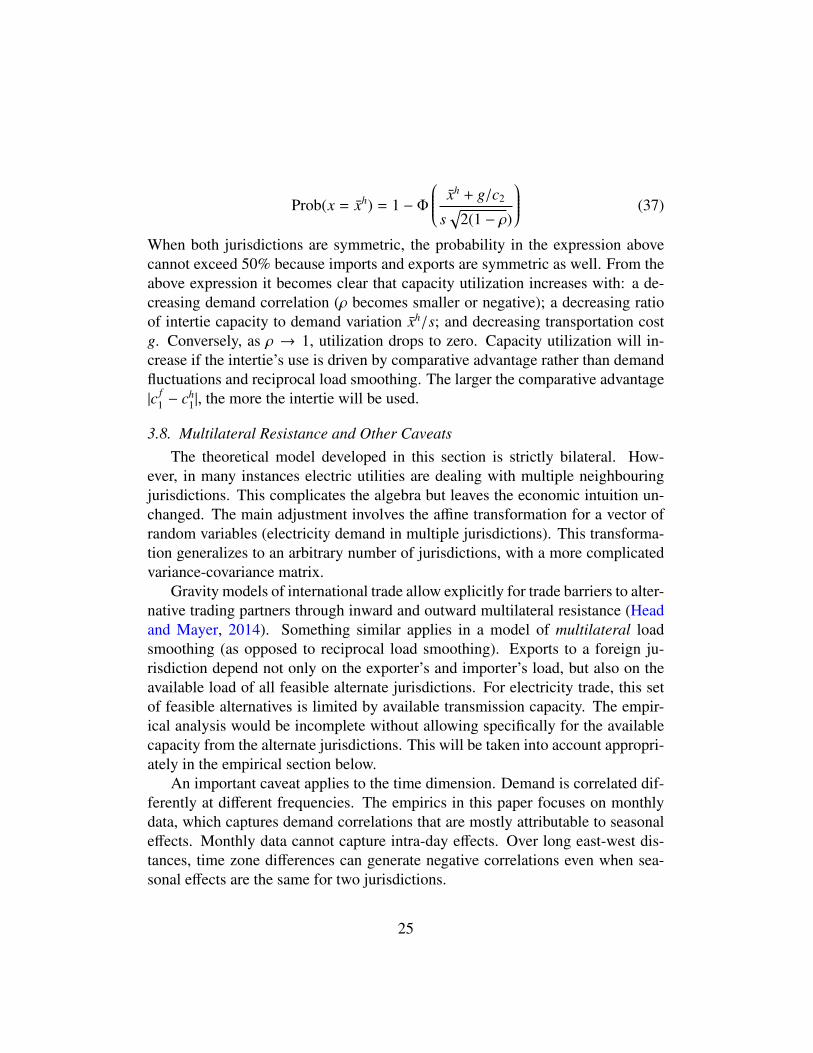
The probability that the capacity is fully utilized in the export direction is thus1 − Φ((c − u)/v). When both jurisdictions are cost-identical and have demandcorrelation ρ, the probability of full intertie utilization is

10As a practical example, the Total Transfer Capability (TTC) of the Ingledow-Custer intertie(two 500 kV lines) between British Columbia and Washington state is rated at 3,150 MW in thesouthern direction and 2,000 MW in the norther direction. A figure in the Technical Appendixdepicts actual utilization hour-by-hour over a few weeks. The frequent reversal of direction is adefining feature of many interties.

24

Prob(x = xh) = 1 − Φ

xh + g/c2

s√

2(1 − ρ)

(37)

When both jurisdictions are symmetric, the probability in the expression abovecannot exceed 50% because imports and exports are symmetric as well. From theabove expression it becomes clear that capacity utilization increases with: a de-creasing demand correlation (ρ becomes smaller or negative); a decreasing ratioof intertie capacity to demand variation xh/s; and decreasing transportation costg. Conversely, as ρ → 1, utilization drops to zero. Capacity utilization will in-crease if the intertie’s use is driven by comparative advantage rather than demandfluctuations and reciprocal load smoothing. The larger the comparative advantage|c f

1 − ch1|, the more the intertie will be used.

3.8. Multilateral Resistance and Other CaveatsThe theoretical model developed in this section is strictly bilateral. How-

ever, in many instances electric utilities are dealing with multiple neighbouringjurisdictions. This complicates the algebra but leaves the economic intuition un-changed. The main adjustment involves the affine transformation for a vector ofrandom variables (electricity demand in multiple jurisdictions). This transforma-tion generalizes to an arbitrary number of jurisdictions, with a more complicatedvariance-covariance matrix.

Gravity models of international trade allow explicitly for trade barriers to alter-native trading partners through inward and outward multilateral resistance (Headand Mayer, 2014). Something similar applies in a model of multilateral loadsmoothing (as opposed to reciprocal load smoothing). Exports to a foreign ju-risdiction depend not only on the exporter’s and importer’s load, but also on theavailable load of all feasible alternate jurisdictions. For electricity trade, this setof feasible alternatives is limited by available transmission capacity. The empir-ical analysis would be incomplete without allowing specifically for the availablecapacity from the alternate jurisdictions. This will be taken into account appropri-ately in the empirical section below.

An important caveat applies to the time dimension. Demand is correlated dif-ferently at different frequencies. The empirics in this paper focuses on monthlydata, which captures demand correlations that are mostly attributable to seasonaleffects. Monthly data cannot capture intra-day effects. Over long east-west dis-tances, time zone differences can generate negative correlations even when sea-sonal effects are the same for two jurisdictions.

25

4. Estimating Electricity Trade

4.1. Principal Estimating EquationThe theory section of this paper has developed a model of two-way trade in

electricity. Equation (13) predicts instantaneous exports and equation (19) pre-dicts the volume of exports from Home to Foreign over a reference time period.The latter equation can be turned into an estimating equation for monthly or an-nual trade in electricity.

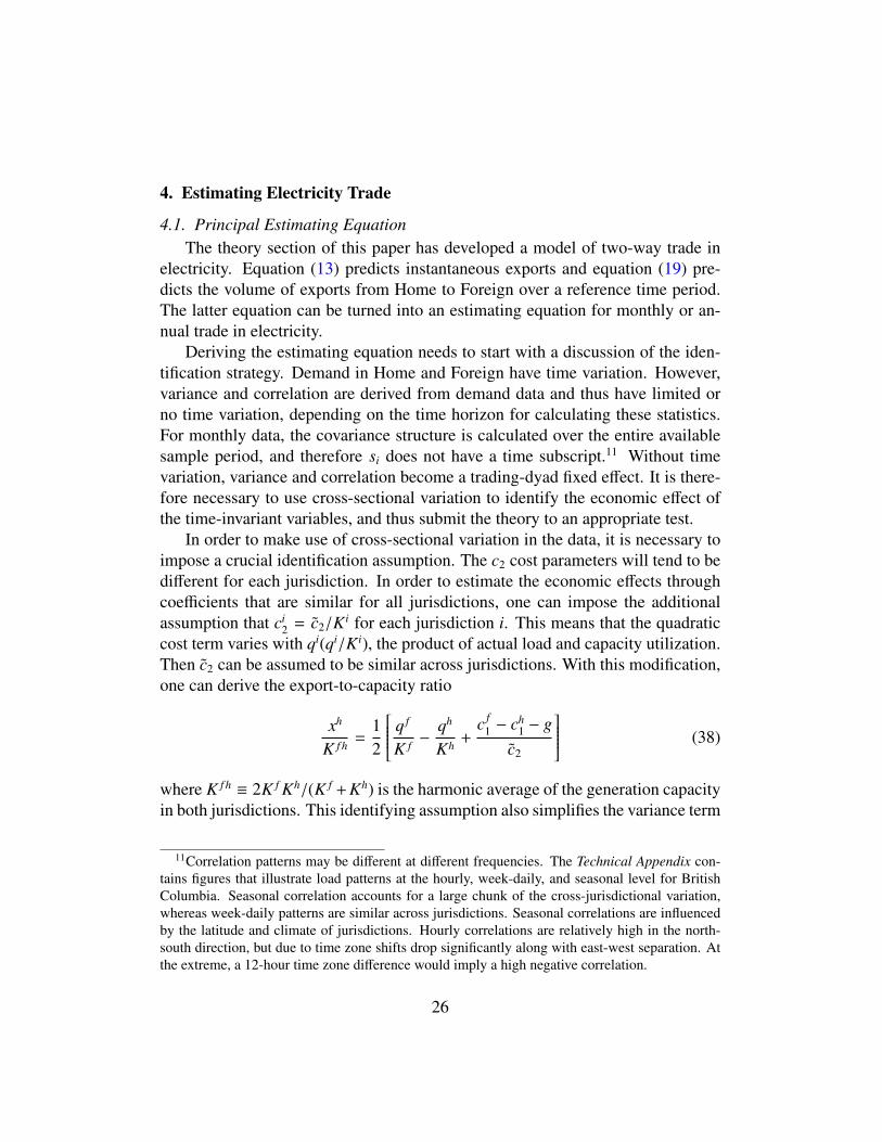
Deriving the estimating equation needs to start with a discussion of the iden-tification strategy. Demand in Home and Foreign have time variation. However,variance and correlation are derived from demand data and thus have limited orno time variation, depending on the time horizon for calculating these statistics.For monthly data, the covariance structure is calculated over the entire availablesample period, and therefore si does not have a time subscript.11 Without timevariation, variance and correlation become a trading-dyad fixed effect. It is there-fore necessary to use cross-sectional variation to identify the economic effect ofthe time-invariant variables, and thus submit the theory to an appropriate test.

In order to make use of cross-sectional variation in the data, it is necessary toimpose a crucial identification assumption. The c2 cost parameters will tend to bedifferent for each jurisdiction. In order to estimate the economic effects throughcoefficients that are similar for all jurisdictions, one can impose the additionalassumption that ci

2 = c2/Ki for each jurisdiction i. This means that the quadraticcost term varies with qi(qi/Ki), the product of actual load and capacity utilization.Then c2 can be assumed to be similar across jurisdictions. With this modification,one can derive the export-to-capacity ratio

xh

K f h =12

q f

K f −qh

Kh +c f

1 − ch1 − g

c2

(38)

where K f h ≡ 2K f Kh/(K f +Kh) is the harmonic average of the generation capacityin both jurisdictions. This identifying assumption also simplifies the variance term

11Correlation patterns may be different at different frequencies. The Technical Appendix con-tains figures that illustrate load patterns at the hourly, week-daily, and seasonal level for BritishColumbia. Seasonal correlation accounts for a large chunk of the cross-jurisdictional variation,whereas week-daily patterns are similar across jurisdictions. Seasonal correlations are influencedby the latitude and climate of jurisdictions. Hourly correlations are relatively high in the north-south direction, but due to time zone shifts drop significantly along with east-west separation. Atthe extreme, a 12-hour time zone difference would imply a high negative correlation.

26

so that it depends merely on the correlation coefficient ρ and the two normalizeddemand standard deviations (si/Ki and s j/K j).

Econometric estimation of trade models often involves ‘gravity’ models of thetype pioneered by Anderson and van Wincoop (2003, 2004). As discussed in Headand Mayer (2014), state-of-the-art estimation techniques typically make use of ex-tensive dyadic fixed effects, which identify economic effects primarily through thetime variation in the trade data. While this approach is necessary because of thepresence of multilateral resistance effects in the love-of-variety models of trade indifferentiated products, it is not strictly necessary in the case of estimating equa-tion (19). Even though the estimating equation has pair-specific effects, they canbe captured through suitable economic variables. Unlike multilateral resistance,these pair-specific effects are generally observable.

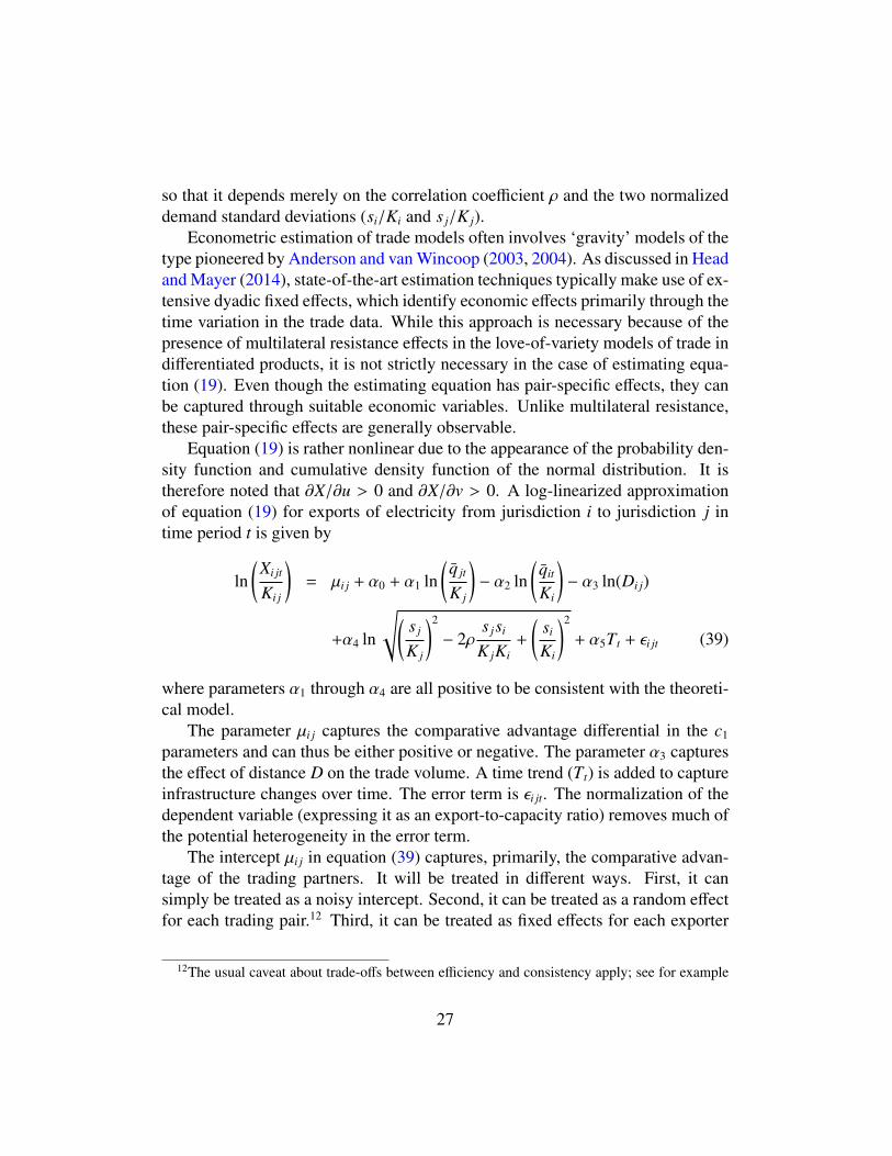
Equation (19) is rather nonlinear due to the appearance of the probability den-sity function and cumulative density function of the normal distribution. It istherefore noted that ∂X/∂u > 0 and ∂X/∂v > 0. A log-linearized approximationof equation (19) for exports of electricity from jurisdiction i to jurisdiction j intime period t is given by

ln(

Xi jt

Ki j

)= µi j + α0 + α1 ln

(q jt

K j

)− α2 ln

(qit

Ki

)− α3 ln(Di j)

+α4 ln

√(s j

K j

)2

− 2ρs jsi

K jKi+

(si

Ki

)2

+ α5Tt + εi jt (39)

where parameters α1 through α4 are all positive to be consistent with the theoreti-cal model.

The parameter µi j captures the comparative advantage differential in the c1

parameters and can thus be either positive or negative. The parameter α3 capturesthe effect of distance D on the trade volume. A time trend (Tt) is added to captureinfrastructure changes over time. The error term is εi jt. The normalization of thedependent variable (expressing it as an export-to-capacity ratio) removes much ofthe potential heterogeneity in the error term.

The intercept µi j in equation (39) captures, primarily, the comparative advan-tage of the trading partners. It will be treated in different ways. First, it cansimply be treated as a noisy intercept. Second, it can be treated as a random effectfor each trading pair.12 Third, it can be treated as fixed effects for each exporter

12The usual caveat about trade-offs between efficiency and consistency apply; see for example

27

and importer (i.e., separate µi and µ j). Fourth, µi j can be modeled explicitly withdeterminants of comparative advantage. Specifically, comparative advantage canbe approximated by the composition of electricity generation, assuming similarunderlying technologies. The composition of generation capacity by type (hy-droelectricity, nuclear, coal, natural gas, other fossil fuel, and renewable sources)can be used to capture the underlying comparative advantage. All four empiricalstrategies are pursued, although with different level of emphasis, and with someresults relegated to the Technical Appendix.13

Lastly, the bilateral identification strategy in equation (39) can be augmentedthrough a a term that mimics ‘multilateral resistance’ in multilateral models oftrade in differentiated goods. In some specification, a variable is included that isthe capacity-weighted average of load factors of the alternate jurisdictions. In theabsence of intra-US state-level trade data, alternate jurisdictions are identified asstates within the same interconnection.

4.2. Estimating Trade Intensity and Export PricesA more indirect method for estimating cross-border trade in electricity focuses

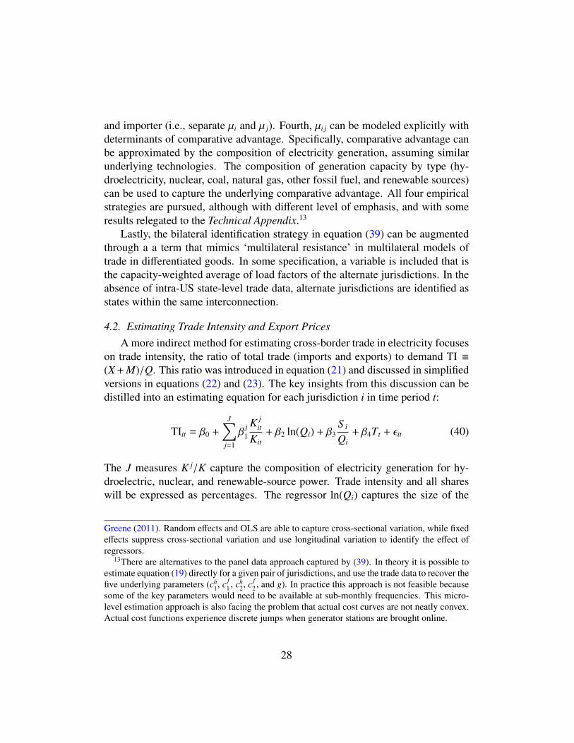
on trade intensity, the ratio of total trade (imports and exports) to demand TI ≡(X+M)/Q. This ratio was introduced in equation (21) and discussed in simplifiedversions in equations (22) and (23). The key insights from this discussion can bedistilled into an estimating equation for each jurisdiction i in time period t:

TIit = β0 +

J∑j=1

βj1

K jit

Kit+ β2 ln(Qi) + β3

S i

Qi+ β4Tt + εit (40)

The J measures K j/K capture the composition of electricity generation for hy-droelectric, nuclear, and renewable-source power. Trade intensity and all shareswill be expressed as percentages. The regressor ln(Qi) captures the size of the

Greene (2011). Random effects and OLS are able to capture cross-sectional variation, while fixedeffects suppress cross-sectional variation and use longitudinal variation to identify the effect ofregressors.

13There are alternatives to the panel data approach captured by (39). In theory it is possible toestimate equation (19) directly for a given pair of jurisdictions, and use the trade data to recover thefive underlying parameters (ch

1, c f1 , ch

2, c f2 , and g). In practice this approach is not feasible because

some of the key parameters would need to be available at sub-monthly frequencies. This micro-level estimation approach is also facing the problem that actual cost curves are not neatly convex.Actual cost functions experience discrete jumps when generator stations are brought online.

28

jurisdiction, and the coefficient of variation S i/Qi captures the demand variabilityof a jurisdiction. The two measures S i and Qi are time-averaged over the sampleperiod. A time trend Tt (time in years before or after 2005.0) is added to captureinfrastructure changes that include grid expansion. Note that changes in compo-sition are captured by the time variation in K j

it.Because states and provinces are of significantly different economic size, it

is meaningful to weight the regressions accordingly. The reported results willemploy weighted least squares with Qi as weights. Data from the United Statesand Canada cannot be pooled. Whereas Canada records electricity imports andexports directly, the US trade intensity is imputed as the absolute difference ofdemand and supply in a given period. This imputation procedure underestimatesactual electricity trade due to aggregation bias.

A further method for testing the model is through the use of the price equa-tion (12). Export prices are influenced positively by increasing load in both ex-porter and importer jurisdiction. Prices should also increase with distance. Equa-tion (12) can be estimated linearly, but a log-linear version may be more appro-priate given that prices often have a long upper tail.

ln(pi jt) = γ0 + µi + µ j + γ1Tt + γ2 ln(q jt

K j

)+ γ3 ln

(qit

Ki

)+ γ4 ln(Di j) + εi jt (41)

There are indicator variables µi and µ j for all exporters and importers, with oneexporter and one importer jurisdiction each excluded as the base. To be consistentwith theory, the estimates of γ2, γ3, and γ4 all have to be positive.

4.3. DataFor all data sources, trade in electricity is defined as Harmonized System (HS)

commodity code 271600. The main source of bilateral monthly trade betweenCanadian provinces and US states is the Canadian International MerchandiseTrade database (CIMT) maintained by Statistics Canada. This database recordsexports from individual Canadian provinces to individual US states, although im-ports into Canadian provinces are only accounted for in aggregate for all US states.The CIMT database records trade data since 1988.

Electricity demand and generation as well as inter-provincial trade in electric-ity has been obtained from Statistics Canada’s CANSIM database. The tables usedinclude 172-0003 (electric power generation, receipts, deliveries and availabilityof electricity, monthly from January 2008 onward) and 127-0008 (correspondingannual data). Profiles of electricity generation by type are available in tables 127-

29

0002 (monthly) and 127-0007 (annual). Table 127-0001 (terminated) containsmonthly electric power statistics from 1950 through 2007. The data reported inthese tables originates with Canada’s National Energy Board.

Additional international trade in electricity data was obtained from the UnitedNations COMTRADE database. This database records both volume and value ofexports and imports, going back to 1988.14

State-level electricity data in the United States are available from the Electric-ity Data Browser of the U.S. Energy Information Administration. State-level dataare estimated and aggregated from reporting utilities and power generation facil-ities. Monthly data are available from January 2001 onwards. Available tablescover generation, consumption, but unfortunately not inter-state deliveries.

Distances between jurisdictions were calculated as population-weighted har-monic averages based on populations and geographic locations of postal codes(United States: ZIP codes; Canada: FSA codes). The Technical Appendix con-tains a table for distances between Canadian provinces and US states.

5. Results

5.1. Testing the Two-Way Model of Electricity TradeThe results for the principal estimating equation are shown in table 4. The

selected sample in the three columns involve three Canadian provinces (BritishColumbia [BC], Ontario [ON], and Manitoba [MB]) exporting electricity to USimporter states. The three provinces were selected because they exhibit signifi-cant levels of two-way trade. Other provinces have little trade or are subject to re-exporting. For example, the province of Quebec exports large quantities of elec-tricity generated outside its boundaries in Labrador. Including such re-exportersconfounds the empirical analysis.

The ordinary least squares (OLS) regressions in table 4 capture about a thirdof the overall variation in the data. The estimates clearly support the theory: allsigns are estimated exactly as expected. An increased load ratio in the importing

14Data prior to 2000 appears rather spotty, and there may be serious data quality issues. Whereasthe value data appears to be mostly reliable, the volume information is often internally inconsistent.This means that exports reported by an origin country to a destination country are rather differentthan imports reported by the destination country from the origin country. While in some cases thisseems to be a misreported physical units problem (MWh instead of GWh), in other cases thereseem to be systematic problems. The volume data in the The COMTRADE database should onlybe used with considerable caution.

30

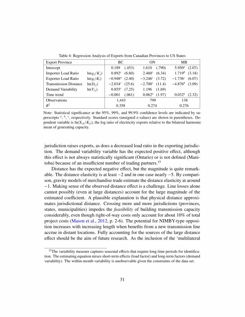
Table 4: Regression Analysis of Exports from Canadian Provinces to US States

Export Province BC ON MBIntercept 0.189 (.453) 1.610 (.790) 5.950a (2.07)Importer Load Ratio ln(q j/K j) 0.892c (6.60) 2.460c (6.34) 1.719b (3.18)Exporter Load Ratio ln(qi/Ki) −0.948a (2.40) −3.246c (3.72) −1.736c (6.07)Transmission Distance ln(Di j) −2.034c (25.6) −2.700c (11.4) −4.876b (3.09)Demand Variability ln(Vi j) 0.855c (7.25) 1.196 (1.69)Time trend −0.001 (.061) 0.062a (1.97) 0.032a (2.32)Observations 1,443 799 138R2 0.358 0.274 0.276

Note: Statistical significance at the 95%, 99%, and 99.9% confidence levels are indicated by su-perscripts a, b, c, respectively. Standard scores (unsigned z-values) are shown in parentheses. De-pendent variable is ln(Xi jt/Ki j), the log ratio of electricity exports relative to the bilateral harmonicmean of generating capacity.

jurisdiction raises exports, as does a decreased load ratio in the exporting jurisdic-tion. The demand variability variable has the expected positive effect, althoughthis effect is not always statistically significant (Ontario) or is not defined (Mani-toba) because of an insufficient number of trading partners.15

Distance has the expected negative effect, but the magnitude is quite remark-able. The distance elasticity is at least −2 and in one case nearly −5. By compari-son, gravity models of merchandise trade estimate the distance elasticity at around−1. Making sense of the observed distance effect is a challenge. Line losses alonecannot possibly (even at large distances) account for the large magnitude of theestimated coefficient. A plausible explanation is that physical distance approxi-mates jurisdictional distance. Crossing more and more jurisdictions (provinces,states, municipalities) impedes the feasibility of building transmission capacityconsiderably, even though right-of-way costs only account for about 10% of totalproject costs (Mason et al., 2012, p. 2-6). The potential for NIMBY-type opposi-tion increases with increasing length when benefits from a new transmission lineaccrue in distant locations. Fully accounting for the sources of the large distanceeffect should be the aim of future research. As the inclusion of the ‘multilateral

15The variability measure captures seasonal effects that require long time periods for identifica-tion. The estimating equation mixes short-term effects (load factor) and long-term factors (demandvariability). The within-month variability is unobservable given the constraints of the data set.

31

resistance’ term in the third column in table 6 documents, the large distance effectis not merely an artifact that results from neglecting the multilateral dimension ofelectricity trade.

Tables 5 and 6 provide further analyses of the estimating equation. Table 5provides simple estimates of the comparative advantage for all trading pairs andseparately for British Columbia (BC) and Ontario (ON). The distance elasticitiesare again around −2. Comparative advantages are captured by proxies for thecomposition of generating capacity, for both exporters and importers in the firstcolumn, and only for the importer for the second and third column that covera single exporter jurisdiction. These estimated effects tend to be significant inthe ‘all’ and ‘BC’ columns. The estimated exporter advantage for hydroelectricpower makes immediate sense, although the negative effect for nuclear powerless so. Only Ontario has a significant amount of nuclear capacity, and thus theeffect may simply capture an Ontario-specific effect. On the importer side, theexcluded category for generation capacity is oil-based power plants (typically withhigh marginal costs). All the importer composition effects are positive in thefirst two columns. It makes sense that a higher proportion of renewable energywould promote a higher level of electricity imports because of the intermittencyof renewable sources. In the case of coal, the effect is negative for Ontario andpositive for British Columbia.

Table 6 explores an integrated framework with regressors for comparative ad-vantage and reciprocal load smoothing. The first column employs the generationcomposition variables as proxies for comparative advantage, while the secondcolumn uses a full set of exporter and importer indicator variables similar to es-timating equation (41). The third column adds a ‘multilateral resistance’ controlvariable as defined earlier (as jurisdiction fixed effects do not capture time vari-ation in loads of alternate jurisdictions). The effect from the load ratios of theexporter and importer are fully consistent with the theory, as is the distance esti-mate. The demand variability regressor is positive but not significant in the firstand third columns, and negative and significant in the second column. The latter isnot consistent with the theory. However, unlike Di j, the variation in Vi j can be cap-tured nearly perfectly with the exporter and importer dummy variables, and thusmulticollinearity may interfere with estimating Vi j correctly in the second column.The introduction of the ‘multilateral resistance’ term for the average load ratio ofalternate import sources strengthens the effect from the exporter and importer loadratios, and itself is negative. This means that alternate electricity sources competewith the exporter region, just as one might expect in a multilateral setting. TheTechnical Appendix reports additional estimates that employ random effects for

32

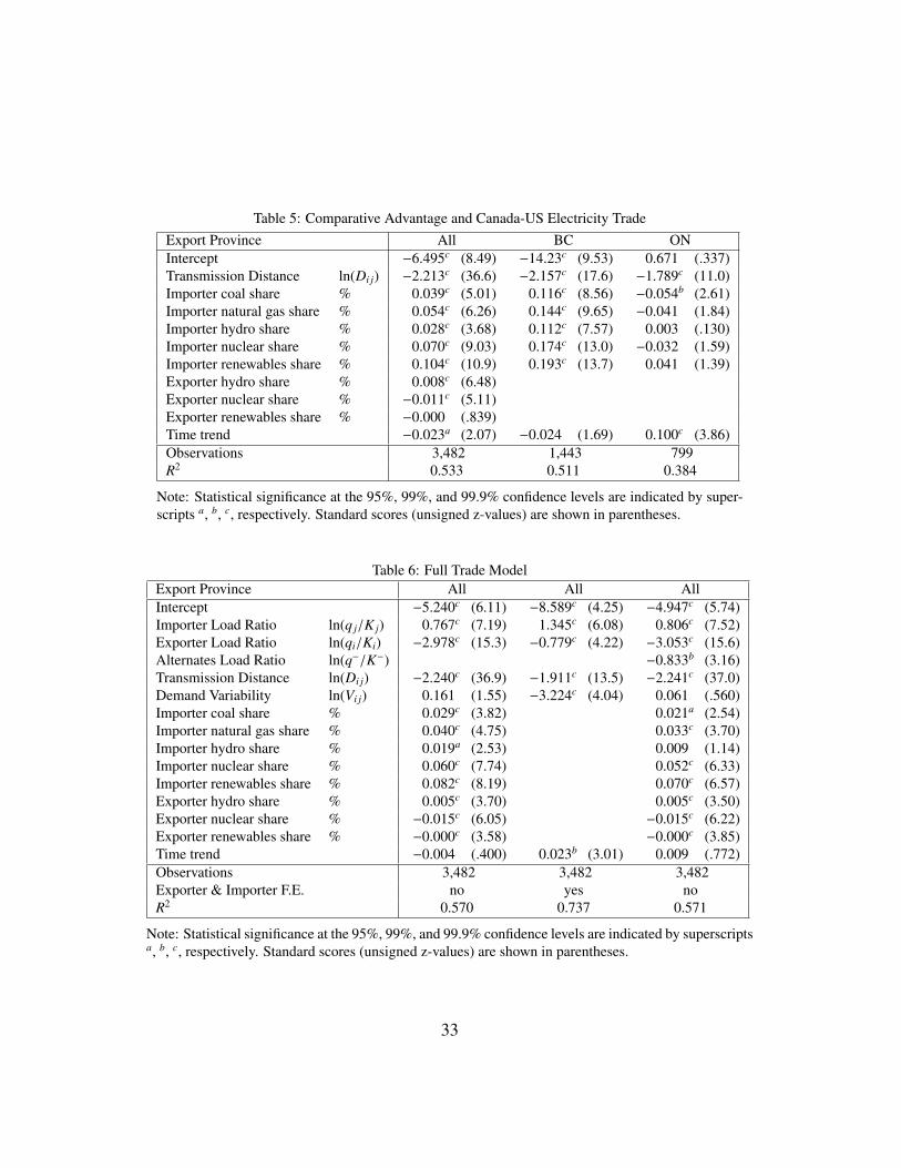
Table 5: Comparative Advantage and Canada-US Electricity TradeExport Province All BC ONIntercept −6.495c (8.49) −14.23c (9.53) 0.671 (.337)Transmission Distance ln(Di j) −2.213c (36.6) −2.157c (17.6) −1.789c (11.0)Importer coal share % 0.039c (5.01) 0.116c (8.56) −0.054b (2.61)Importer natural gas share % 0.054c (6.26) 0.144c (9.65) −0.041 (1.84)Importer hydro share % 0.028c (3.68) 0.112c (7.57) 0.003 (.130)Importer nuclear share % 0.070c (9.03) 0.174c (13.0) −0.032 (1.59)Importer renewables share % 0.104c (10.9) 0.193c (13.7) 0.041 (1.39)Exporter hydro share % 0.008c (6.48)Exporter nuclear share % −0.011c (5.11)Exporter renewables share % −0.000 (.839)Time trend −0.023a (2.07) −0.024 (1.69) 0.100c (3.86)Observations 3,482 1,443 799R2 0.533 0.511 0.384

Note: Statistical significance at the 95%, 99%, and 99.9% confidence levels are indicated by super-scripts a, b, c, respectively. Standard scores (unsigned z-values) are shown in parentheses.

Table 6: Full Trade ModelExport Province All All AllIntercept −5.240c (6.11) −8.589c (4.25) −4.947c (5.74)Importer Load Ratio ln(q j/K j) 0.767c (7.19) 1.345c (6.08) 0.806c (7.52)Exporter Load Ratio ln(qi/Ki) −2.978c (15.3) −0.779c (4.22) −3.053c (15.6)Alternates Load Ratio ln(q−/K−) −0.833b (3.16)Transmission Distance ln(Di j) −2.240c (36.9) −1.911c (13.5) −2.241c (37.0)Demand Variability ln(Vi j) 0.161 (1.55) −3.224c (4.04) 0.061 (.560)Importer coal share % 0.029c (3.82) 0.021a (2.54)Importer natural gas share % 0.040c (4.75) 0.033c (3.70)Importer hydro share % 0.019a (2.53) 0.009 (1.14)Importer nuclear share % 0.060c (7.74) 0.052c (6.33)Importer renewables share % 0.082c (8.19) 0.070c (6.57)Exporter hydro share % 0.005c (3.70) 0.005c (3.50)Exporter nuclear share % −0.015c (6.05) −0.015c (6.22)Exporter renewables share % −0.000c (3.58) −0.000c (3.85)Time trend −0.004 (.400) 0.023b (3.01) 0.009 (.772)Observations 3,482 3,482 3,482Exporter & Importer F.E. no yes noR2 0.570 0.737 0.571

Note: Statistical significance at the 95%, 99%, and 99.9% confidence levels are indicated by superscriptsa, b, c, respectively. Standard scores (unsigned z-values) are shown in parentheses.

33

the full panel. Qualitatively, the results are highly similar to those reported here.

5.2. The Extensive Margin of TradeCross-border trade in electricity exhibits different extensive margins. First is

the margin of exporting and importing on a jurisdictional level: which province-state dyads trade, and which do not. This type of margin is quite dominant as eachexporting province only has a relatively small number of import partners in theUnited States. A logistic regression was used to explore the first type of margin.The results are reported in the Technical Appendix because they shed little addi-tional light on cross-border trade in electricity. This analysis looks at all possibletrading dyads (all provinces times all states); only about 5% of them trade. Thisanalysis is purely cross-sectional and does not include a time dimension. Only thedistance effect is estimated significantly along with a negative effect from a highershare or renewables in the exporter jurisdiction. As can be expected, distance andavailability of transmission infrastructure determine trading capability. The sep-aration into different interconnections is, of course, a nearly perfect predictor ofwho can trade with whom.

Another type of margin is within the group of trading dyads. Some dyadsdo not always trade. There may be significant periods of zero trade for a giventrading pair. These may indicate periods when trading is not profitable despitethe fact that transmission capacity exists. This type of extensive margin is relatedto economic rather than physical constraints. This type of margin is consistentwith two-way trade in electricity and the no-trade gap in figure 8. However, thismargin is difficult to identify in monthly data. Aggregation may obscure what maybe episodes of zero trade throughout a month. If trade is more one-way (drivenby comparative advantage) than two-way (driven by reciprocal load smoothing),transmission capacity will also tend to be more utilized.

5.3. Trade IntensityThe theory of reciprocal load smoothing can also be tested through estimating

equation (40) for trade intensity. Tables 7 and 8 report the results of this approachfor Canada and the United States, respectively. Because of the vastly differentsize of jurisdictions (especially in Canada), weighted least squares were used toobtain estimates, with average jurisdictional demand as the weight. The first col-umn in both tables includes all jurisdictions. As a robustness check, the secondcolumn suppresses observations with trade intensities in excess of 120%, whichis indicative of jurisdictions that produce electricity primarily for export. Thethird column suppresses observations where the trade intensity is zero (Canada)

34

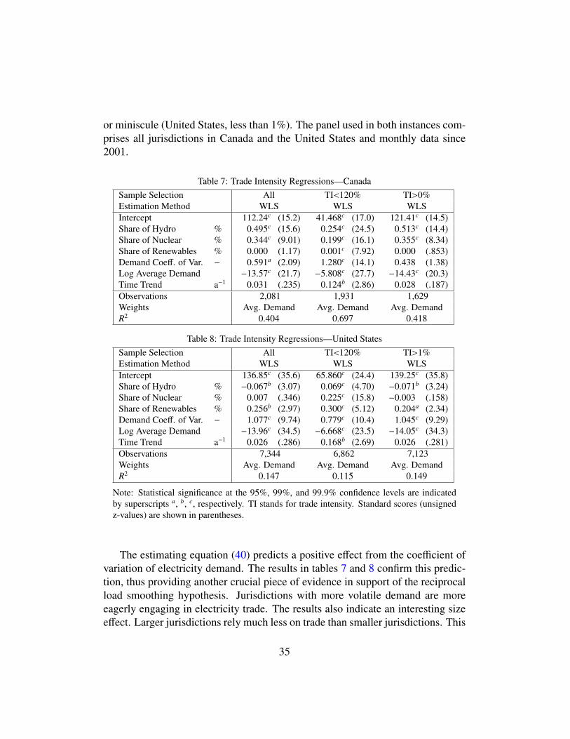
or miniscule (United States, less than 1%). The panel used in both instances com-prises all jurisdictions in Canada and the United States and monthly data since2001.

Table 7: Trade Intensity Regressions—CanadaSample Selection All TI<120% TI>0%Estimation Method WLS WLS WLSIntercept 112.24c (15.2) 41.468c (17.0) 121.41c (14.5)Share of Hydro % 0.495c (15.6) 0.254c (24.5) 0.513c (14.4)Share of Nuclear % 0.344c (9.01) 0.199c (16.1) 0.355c (8.34)Share of Renewables % 0.000 (1.17) 0.001c (7.92) 0.000 (.853)Demand Coeff. of Var. − 0.591a (2.09) 1.280c (14.1) 0.438 (1.38)Log Average Demand −13.57c (21.7) −5.808c (27.7) −14.43c (20.3)Time Trend a−1 0.031 (.235) 0.124b (2.86) 0.028 (.187)Observations 2,081 1,931 1,629Weights Avg. Demand Avg. Demand Avg. DemandR2 0.404 0.697 0.418

Table 8: Trade Intensity Regressions—United StatesSample Selection All TI<120% TI>1%Estimation Method WLS WLS WLSIntercept 136.85c (35.6) 65.860c (24.4) 139.25c (35.8)Share of Hydro % −0.067b (3.07) 0.069c (4.70) −0.071b (3.24)Share of Nuclear % 0.007 (.346) 0.225c (15.8) −0.003 (.158)Share of Renewables % 0.256b (2.97) 0.300c (5.12) 0.204a (2.34)Demand Coeff. of Var. − 1.077c (9.74) 0.779c (10.4) 1.045c (9.29)Log Average Demand −13.96c (34.5) −6.668c (23.5) −14.05c (34.3)Time Trend a−1 0.026 (.286) 0.168b (2.69) 0.026 (.281)Observations 7,344 6,862 7,123Weights Avg. Demand Avg. Demand Avg. DemandR2 0.147 0.115 0.149

Note: Statistical significance at the 95%, 99%, and 99.9% confidence levels are indicatedby superscripts a, b, c, respectively. TI stands for trade intensity. Standard scores (unsignedz-values) are shown in parentheses.

The estimating equation (40) predicts a positive effect from the coefficient ofvariation of electricity demand. The results in tables 7 and 8 confirm this predic-tion, thus providing another crucial piece of evidence in support of the reciprocalload smoothing hypothesis. Jurisdictions with more volatile demand are moreeagerly engaging in electricity trade. The results also indicate an interesting sizeeffect. Larger jurisdictions rely much less on trade than smaller jurisdictions. This

35

makes intuitive sense. Larger jurisdictions tend to be more diversified in terms ofgenerating capacity and may be better able to balance load in different regions.Smaller jurisdictions need to rely more on their neighbours to compensate forfluctuating demand, or simply import electricity from their bigger neighbours.

In Canada, jurisdictions with a higher proportion of hydroelectric and nuclearpower tend to increase their trade intensity. This may be an indication of the com-parative advantage of these technologies, or the higher reliability and availabilityfor satisfying base loads. In the United States, these two power sources do notseem to have a large influence on the trade intensity. However, a larger share ofrenewable energy is clearly associated with an increase in electricity trade.

5.4. Export PricesThe Canadian International Merchandise Trade (CIMT) database records both

volume and value of exports and imports. It is therefore possible to analyze theprice dimension of exports. Summary data appear in the Technical Appendix.There is significant variation in prices along with occasional price spikes such asthose during the 2000-2001 California electricity crisis.16 Price spikes in excessof $200/MWh were purposefully excluded from the analysis in this section.

Table 9 reports results for the price estimating equation (41), which includesfixed effects for exporter provinces and importer states. It may be interesting tolook at these numbers as they indicate idiosyncratic price premia and discounts. Inthe table the importer states are prefixed M, and the exporter provinces ar prefixedX. The base exporter province is Ontario, and the base importer state is New York;all price premia are relative to this base-pair.

The first column in table 9 reports simple OLS estimates. The second col-umn (QREG) reports results from a quantile regression of the median to allow forthe long tail of the price distribution. The dependent variable in both columns isexpressed in dollars per MWh. The third—and preferred—estimation approachcorresponds directly to the log-linear estimating equation (41). The estimated co-efficients of the exporter and importer load ratios are both positive, fully consistentwith theory. The effect of distance cannot be estimated significantly in the pre-ferred specification, although it points in the right direction. Other specificationssuggests that the distance effect is indeed positive as predicted.17 There is also a

16See Borenstein (2002) for a discussion of the factors that contributed to the California elec-tricity crisis.

17The Technical Appendix contains a table with robustness checks where the distance effect isestimated significantly with a positive sign when the importer dummies are excluded and only

36

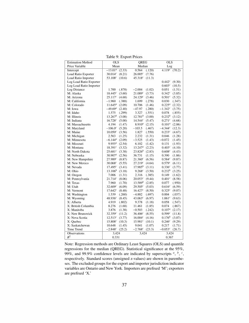
Table 9: Export PricesEstimation Method OLS QREG OLSPrice Variable Mean Median LogIntercept −13.01a (2.33) 0.564 (.120) 4.119c (70.2)Load Ratio Exporter 30.014c (8.21) 26.005c (7.76)Load Ratio Importer 53.108c (10.6) 45.318c (11.3)Log Load Ratio Exporter 0.442c (9.30)Log Load Ratio Importer 0.603c (10.5)Log Distance 1.700 (.878) −2.004 (1.02) 0.051 (1.51)M: Alaska 18.445c (3.60) 21.089c (3.73) 0.342c (3.85)M: Arizona 25.117c (4.68) 24.129c (3.46) 0.501c (5.32)M: California −1.960 (.388) 1.699 (.278) 0.030 (.347)M: Colorado 11.645a (2.09) 10.706 (1.46) 0.225a (2.32)M: Iowa −49.69a (2.40) −47.97 (.280) −1.342c (3.75)M: Idaho 1.575 (.299) 3.327 (.551) 0.078 (.855)M: Illinois 13.267b (3.08) 12.781b (3.00) 0.232b (3.12)M: Indiana 16.728c (5.00) 14.544c (5.47) 0.271c (4.68)M: Massachusetts 4.194 (1.47) 8.910a (2.15) 0.101a (2.06)M: Maryland −106.0c (5.20) −103.5 (.467) −4.344c (12.3)M: Maine 10.050c (3.56) 1.827 (.550) 0.233c (4.67)M: Michigan 2.563 (1.25) 2.232 (1.31) 0.046 (1.28)M: Minnesota −6.144a (2.09) −3.525 (1.43) −0.072 (1.45)M: Missouri 9.955a (2.54) 6.102 (1.42) 0.131 (1.93)M: Montana 18.391c (3.32) 13.247a (2.23) 0.403c (4.10)M: North Dakota 25.681c (3.38) 23.826b (2.83) 0.608c (4.43)M: Nebraska 30.907a (2.56) 36.731 (1.15) 0.390 (1.86)M: New Hampshire 27.989c (8.87) 21.360c (6.56) 0.584c (9.87)M: New Mexico 30.068c (5.55) 27.219c (4.64) 0.579c (6.11)M: Nevada 17.495c (3.41) 17.985b (3.11) 0.336c (3.77)M: Ohio 13.106b (3.18) 9.268c (3.50) 0.232b (3.25)M: Oregon 7.006 (1.31) 2.316 (.385) 0.149 (1.62)M: Pennsylvania 21.714c (8.06) 20.053c (9.44) 0.401c (8.58)M: Texas 7.960 (1.70) 13.589b (2.85) 0.077 (.950)M: Utah 32.609c (6.09) 29.505c (5.03) 0.616c (6.59)M: Vermont 17.642c (8.48) 16.427c (8.50) 0.325c (9.07)M: Washington 1.539 (.260) −4.882 (.697) 0.004 (.037)M: Wyoming 48.936c (8.45) 43.063c (6.97) 1.061c (9.63)X: Alberta 4.919 (.802) 9.378 (1.18) 0.058 (.547)X: British Columbia 8.276 (1.68) 11.461 (1.85) 0.074 (.867)X: Manitoba 3.876 (1.38) −0.503 (.242) 0.107a (2.17)X: New Brunswick 32.359c (11.2) 36.406c (8.55) 0.599c (11.8)X: Nova Scotia 12.513c (3.77) 16.004c (4.16) 0.176b (3.07)X: Quebec 15.808c (10.3) 15.981c (10.1) 0.246c (9.29)X: Saskatchewan 10.648 (1.45) 9.041 (1.07) 0.217 (1.71)Time Trend −2.848c (25.2) −2.768c (23.3) −0.053c (26.7)Observations 3,424 3,424 3,424R2 0.331 0.367

Note: Regression methods are Ordinary Least Squares (OLS) and quantileregressions for the median (QREG). Statistical significance at the 95%,99%, and 99.9% confidence levels are indicated by superscripts a, b, c,respectively. Standard scores (unsigned z-values) are shown in parenthe-ses. The excluded groups for the export and importer jurisdiction indicatorvariables are Ontario and New York. Importers are prefixed ‘M’; exportersare prefixed ‘X.’

37

negative time trend in the data. Electricity exports tend to get cheaper over time,despite the rising cost of generation. Perhaps power markets in North America arebecoming more efficient in dispatching electricity.

6. The Gains from Electricity Trade

Having laid out a new theory that leads to gains from trade, the obvious ques-tion to ask is about the size of these gains from trade. Does ‘reciprocal loadsmoothing’ generate economically meaningful welfare gains? Fundamentally,these gains come from trading off generation capacity and transmission capacity.Underinvestment in transmission capacity equals overinvestment in generation ca-pacity, and this is economically inefficient. Do potential welfare gains make a casefor pursuing policy changes towards building a North American ‘supergrid’?

The case for increased integration of the North American is gaining significantmomentum (Bowman et al., 2009a,b; Carr, 2010; Goodman, 2010; Baker et al.,2011; Bahar and Sauvage, 2013; Canadian Electricity Association, 2013). Thereare many technical reasons that promote the notion of building a continent-widesupergrid. Chief among them is the integration of renewable energy; see Am-bec and Crampes (2012) and van Kooten et al. (2013) for a discussion of manyof the related issues. A supergrid may also provide greater reliability and redun-dancy. There are numerous institutional issues and economic frictions that holdback the construction of more transmission infrastructure. The most obvious isthe division of the North American transmission system into separate and mostlyself-contained interconnections: a world akin to free trade areas with high tariffwalls between them. Neighbouring states cannot exploit trading opportunities ifthey belong to different interconnections, and more distant states cannot exploitefficiencies from cross-continental delivery of power.

This section cannot provide a concise answer about the current and potentialgains from cross-border electricity trade. Many of the current gains are realizedat the sub-monthly level, and potential future gains from trade are contingent onmodeling increased transmission capacity. However, it is possible to sketch outthe economic extremes of a fully unified grid with pooled supply and zero trans-mission cost, and an autarkic grid where each province or state is self-sufficient.18

In a fully integrated continental grid, local demand would be added up nationally

exporter dummies are used.18A rigorous welfare analysis requires hourly mirco data and a sophisticated simulation-

optimization model in which additional long-distance bulk transmission capacity can be studied.

38

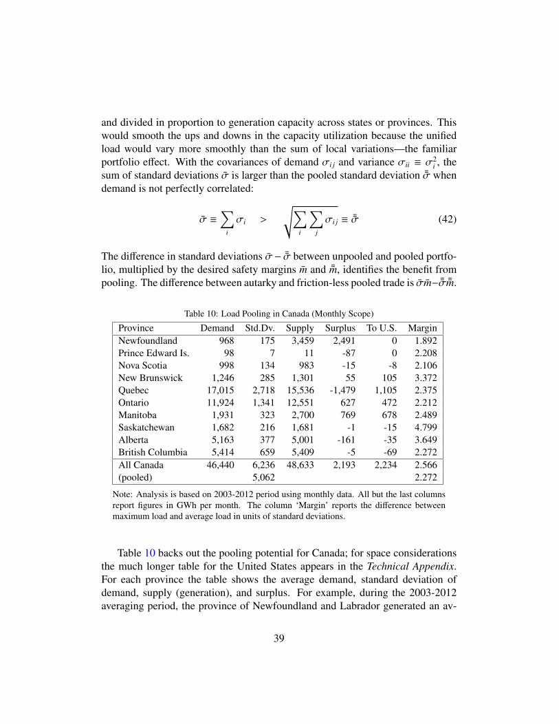
and divided in proportion to generation capacity across states or provinces. Thiswould smooth the ups and downs in the capacity utilization because the unifiedload would vary more smoothly than the sum of local variations—the familiarportfolio effect. With the covariances of demand σi j and variance σii ≡ σ

2i , the

sum of standard deviations σ is larger than the pooled standard deviation ¯σ whendemand is not perfectly correlated:

σ ≡∑

i

σi >

√∑i

∑j

σi j ≡ ¯σ (42)

The difference in standard deviations σ− ¯σ between unpooled and pooled portfo-lio, multiplied by the desired safety margins m and ¯m, identifies the benefit frompooling. The difference between autarky and friction-less pooled trade is σm− ¯σ ¯m.

Table 10: Load Pooling in Canada (Monthly Scope)

Province Demand Std.Dv. Supply Surplus To U.S. MarginNewfoundland 968 175 3,459 2,491 0 1.892Prince Edward Is. 98 7 11 -87 0 2.208Nova Scotia 998 134 983 -15 -8 2.106New Brunswick 1,246 285 1,301 55 105 3.372Quebec 17,015 2,718 15,536 -1,479 1,105 2.375Ontario 11,924 1,341 12,551 627 472 2.212Manitoba 1,931 323 2,700 769 678 2.489Saskatchewan 1,682 216 1,681 -1 -15 4.799Alberta 5,163 377 5,001 -161 -35 3.649British Columbia 5,414 659 5,409 -5 -69 2.272All Canada 46,440 6,236 48,633 2,193 2,234 2.566(pooled) 5,062 2.272

Note: Analysis is based on 2003-2012 period using monthly data. All but the last columnsreport figures in GWh per month. The column ‘Margin’ reports the difference betweenmaximum load and average load in units of standard deviations.

Table 10 backs out the pooling potential for Canada; for space considerationsthe much longer table for the United States appears in the Technical Appendix.For each province the table shows the average demand, standard deviation ofdemand, supply (generation), and surplus. For example, during the 2003-2012averaging period, the province of Newfoundland and Labrador generated an av-

39

erage monthly surplus of 2.5 TWh. Quebec’s generation deficit of 1.5 TWh wasbalanced by importing electricity from Labrador, leaving roughly 1.1 TWh for ex-port to the United States. Canada’s nation-wide surplus of 2.2 TWh was exportedto the United States. The last column shows the safety margin for each province,defined as the difference between maximum and average demand expressed instandard deviations. For example, British Columbia’s required safety margin was2.3 times its standard deviation of 659 GWh; these 1,497 GWh amount to 28% ofthe province’s generating capacity.

The last two lines in table 10 identify the benefits from a nationally pooledgrid. A pooled grid would reduce the standard deviation from σ=6,236 GWh to¯σ=5,062 GWh per month, a remarkable 19% drop. The pooled safety marginis also a bit smaller than the weighted average of the individual safety margins.The required contingent capacity is therefore 11.5 TWh instead of 16.0 TWh permonth. On a nationwide level, the 4.5 TWh/month difference is equivalent in sizeto about seven modern nuclear reactors or a dozen large hydroelectric dams.19 Butjust how much more trade—and intertie capacity—would a nationally-integratedgrid entail? Would the cost of building this intertie capacity come at a lowercost than building seven nuclear reactors (about $50 billion) or a dozen new dams(about $96 billion)?20 Of course, we are clearly not at the point of a fully autarkicsystem as most jurisdictions indeed trade with one or more of their neighbouringjurisdictions. On the other hand, the cost of building new transmission capacitydiminishes the potential for grid integration at the other end of the spectrum.

The equivalent gains from grid integration are significantly larger in the UnitedStates. The pooled standard deviation of demand is 29,567 GWh, compared to35,257 GWh unpooled. After applying the safety margins (2.286 pooled and2.565 unpooled), the efficiency gap is 22.8 TWh/month in reduced contingentcapacity—the equivalent of 28 nuclear reactors or 65 Hoover dams! Of course,the existing grid already realizes some of these gains. Careful analysis is neededto quantify the remaining gap and the competing costs of building more trans-mission capacity versus more generating capacity. The 22.8 TWh/month figureunderestimates the gains from trade because the available monthly data only cap-tures seasonal effects in the north-south direction. Over long distances, east-west

19Figures are based on the Westinghouse AP1000 design, rated at about 600 GWh/month, andthe Hoover dam, which generates about 350 GWh/month.

20This is based on projected costs for the Vogtle plant expansion in Georgia: $14 billion fortwo AP 1000 reactors. By comparison, a new hydroelectric dam in British Columbia, Site C, isexpected to cost about $8 billion and is expected to generate 380 GWh/month.

40

timezone shifts could provide significant additional intra-day gains from trade.A supergrid can provide several other economic and environmental benefits.

In the long term, jurisdictions with a comparative advantage in electricity produc-tion could build up generation capacity if they can deliver their electricity to moredistant markets. Renewable energy sources such as wind also require complemen-tarities in generating capacity to make up for their intermittency. Hydro power(which can accelerate or decelerate use of reservoirs) are a natural complement towind and solar energy. Greater integration can also improve overall system relia-bility. More importantly, integration may also provide an opportunity for retiringpolluting generating capacity. The 22.8 TWh/month efficiency gap in the UnitedStates translates into a significant potential for climate change mitigation. At acarbon dioxide intensity of about 1 tonne per MWh,21 an annual efficiency gap of273 TWh translates into a potential for reducing carbon dioxide emissions by 273million tonnes, or 5.2% of 2012’s annual total of 5.3 billion tonnes.

7. Conclusions

This paper has developed a theoretical model of two-way trade in electricity.The set-up shares a common root in the trade-theoretical ‘reciprocal dumping’model, which provided a foundation for two-way trade in identical commodities.However, the underlying economic logic is fundamentally different for electric-ity trade. The ‘reciprocal dumping’ model relies on reciprocal market access ofoligopolistic competitors in two countries. While this model of two-way trade isdriven by market structure, the two-way trade in electricity is caused by stochas-tic demand that shifts electricity generation up and down on an upward-slopingmarginal cost curve as electric utilities deploy their generation assets on a least-cost-first basis. Neighbouring jurisdictions engage in ‘reciprocal load smoothing.’The theory developed in this paper has identified several key features of two-waytrade in electricity:

• Trade is one-way in the presence of strong (conventional) comparative ad-vantage in electricity production, and trade tends to become more two-waywhen comparative advantages between trading partners are more closelymatched.

21Source: Environmental Protection Agency. 2,249 lbs/MWh for coal-fired power stations inthe United States.

41

• Trade is two-way in the presence of fluctuating demand where exports andimports follow the load difference between two jurisdictions. Trading op-portunities increase with the variability of electricity demand over time (dueto seasonal or intra-day effects) and lower (or negative) correlation in de-mand. Jurisdictional size differences also promote cross-border trade.

The empirical investigation of Canada-US cross-border trade in electricity lendsstrong support to the theoretical model developed in this paper. Conventionalcomparative advantage and reciprocal load smoothing work in tandem to explainthe observed patterns of cross-border trade in electricity.

Empirically, the volume of trade in electricity is subject to a much steeper de-cline over distance than trade in merchandise goods. Whereas the distance elastic-ity for the latter is typically around (negative) unity, it is roughly twice as high forelectricity. Doubling the distance reduces electricity trade by one-fourth. Perhapsphysical distance captures ‘jurisdictional’ distance: the legal and administrativedifficulties of building long-distance interties.

Whether the current level of electricity trade and continental integration of theelectricity grid is sufficient remains a rather important policy question. Roughcalculations of the trade potential—the difference between autarky and completefrictionless integration—suggest an efficiency gap equivalent to 65 Hoover damsin the United States and a dozen hydro dams in Canada. Even if only half or athird of this efficiency gap remains to be closed, the potential gains from moreelectricity trade across jurisdictions are impressive. With long-distance transmis-sion costs falling through the development of high-voltage direct current (HVDC)transmission lines, combined with the need to accommodate increasing volumesof intermittent power from renewable sources, the quadrupling of cross-bordertrade in electricity over the last decade (illustrated in figure 1) is making verygood economic sense.

The theory of ‘reciprocal load smoothing’ introduced in this paper constitutesa new mechanism for gains from trade that may transcend electricity. In princi-ple, the mechanism can apply to any homogenous product provided that there is(a) non-perfect correlation in stochastic demand across trading partners and (b)strongly upward-sloping marginal costs in production.

42

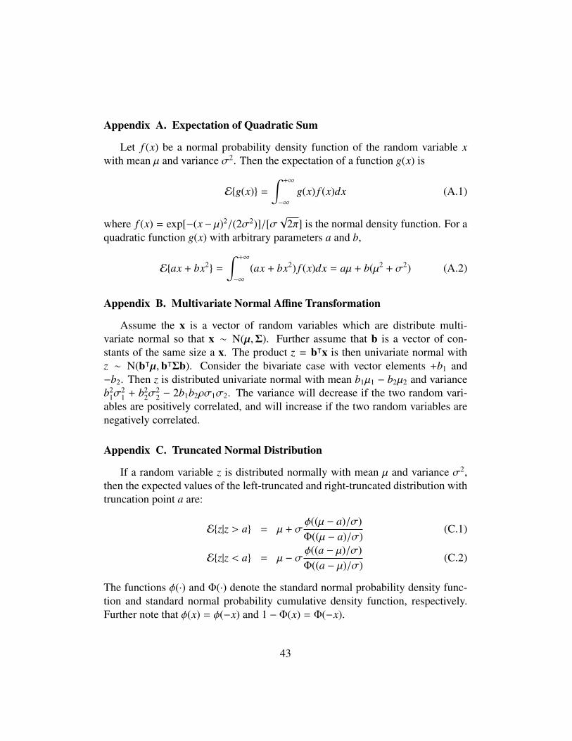
Appendix A. Expectation of Quadratic Sum

Let f (x) be a normal probability density function of the random variable xwith mean µ and variance σ2. Then the expectation of a function g(x) is

E{g(x)} =∫ +∞

−∞

g(x) f (x)dx (A.1)

where f (x) = exp[−(x− µ)2/(2σ2)]/[σ√

2π] is the normal density function. For aquadratic function g(x) with arbitrary parameters a and b,

E{ax + bx2} =

∫ +∞

−∞

(ax + bx2) f (x)dx = aµ + b(µ2 + σ2) (A.2)

Appendix B. Multivariate Normal Affine Transformation

Assume the x is a vector of random variables which are distribute multi-variate normal so that x ∼ N(µ,Σ). Further assume that b is a vector of con-stants of the same size a x. The product z = bᵀx is then univariate normal withz ∼ N(bᵀµ,bᵀΣb). Consider the bivariate case with vector elements +b1 and−b2. Then z is distributed univariate normal with mean b1µ1 − b2µ2 and varianceb2

1σ21 + b2

2σ22 − 2b1b2ρσ1σ2. The variance will decrease if the two random vari-

ables are positively correlated, and will increase if the two random variables arenegatively correlated.

Appendix C. Truncated Normal Distribution

If a random variable z is distributed normally with mean µ and variance σ2,then the expected values of the left-truncated and right-truncated distribution withtruncation point a are:

E{z|z > a} = µ + σφ((µ − a)/σ)Φ((µ − a)/σ)

(C.1)

E{z|z < a} = µ − σφ((a − µ)/σ)Φ((a − µ)/σ)

(C.2)

The functions φ(·) and Φ(·) denote the standard normal probability density func-tion and standard normal probability cumulative density function, respectively.Further note that φ(x) = φ(−x) and 1 − Φ(x) = Φ(−x).

43

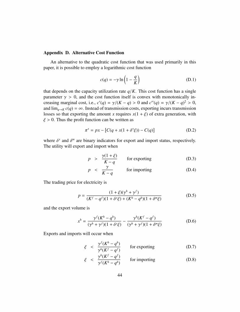
Appendix D. Alternative Cost Function

An alternative to the quadratic cost function that was used primarily in thispaper, it is possible to employ a logarithmic cost function

c(q) = −γ ln(1 −

qK

)(D.1)

that depends on the capacity utilization rate q/K. This cost function has a singleparameter γ > 0, and the cost function itself is convex with monotonically in-creasing marginal cost, i.e., c′(q) = γ/(K − q) > 0 and c′′(q) = γ/(K − q)2 > 0,and limq→K c(q) = ∞. Instead of transmission costs, exporting incurs transmissionlosses so that exporting the amount x requires x(1 + ξ) of extra generation, withξ > 0. Thus the profit function can be written as

πx = px −[C(q + x(1 + δxξ)) −C(q)

](D.2)

where δx and δm are binary indicators for export and import status, respectively.The utility will export and import when

p >γ(1 + ξ)K − q

for exporting (D.3)

p <γ

K − qfor importing (D.4)

The trading price for electricity is

p =(1 + ξ)(γh + γ f )

(K f − q f )(1 + δxξ) + (Kh − qh)(1 + δmξ)(D.5)

and the export volume is

xh =γ f (Kh − qh)

(γh + γ f )(1 + δxξ)−

γh(K f − q f )(γh + γ f )(1 + δmξ)

(D.6)

Exports and imports will occur when

ξ <γ f (Kh − qh)γh(K f − q f )

for exporting (D.7)

ξ <γh(K f − q f )γ f (Kh − qh)

for importing (D.8)

44

From the above it is clear that xh is a linear function of qh and q f , and thus theintegration over the reference time period to find Xh and Mh proceeds in the samefashion as discussed in the paper and Appendix B and Appendix C.

References

Ambec, S., Crampes, C., 2012. Electricity provision with intermittent sourcesof energy. Resource and Energy Economics 34, 319–336. doi:10.1016/j.reseneeco.2012.01.001.

Anderson, J.E., van Wincoop, E., 2003. Gravity with gravitas: A solution tothe border puzzle. American Economic Review 93, 170–192. doi:10.1257/000282803321455214.

Anderson, J.E., van Wincoop, E., 2004. Trade costs. Journal of Economic Litera-ture 42, 691–751. doi:10.1257/0022051042177649.

Bahar, H., Sauvage, J., 2013. Cross-Border Trade in Electricity and the Devel-opment of Renewables-Based Electric Power: Lessons from Europe. Techni-cal Report. OECD. doi:10.1787/5k4869cdwnzr-en. Trade and EnvironmentWorking Papers 2013/02.

Baker, B., Sklokin, I., Coad, L., Crawford, T., 2011. Canada’s Electricity Infras-tructure. Technical Report. The Conference Board of Canada.

Bernard, J.T., Roland, M., 1997. Rent dissipation through electricity prices ofpublicly owned utilities. Canadian Journal of Economics 30, 1204–19. URL:http://www.jstor.org/stable/136317.

Borenstein, S., 2002. The trouble with electricity markets: Understanding cali-fornia’s restructuring disaster. Journal of Economic Perspectives 16, 191–211.doi:10.1257/0895330027175.

Bowman, C.W., Marceau, R.J., Griesbach, R.C., 2009a. Electricity: Interconnect-ing Canada—A Strategic Advantage. Technical Report. Canadian Academy ofEngineering. Ottawa. Volume I: Findings, Conclusions and Recommendations.

Bowman, C.W., Marceau, R.J., Griesbach, R.C., 2009b. Electricity: Interconnect-ing Canada—A Strategic Advantage. Technical Report. Canadian Academy ofEngineering. Ottawa. Volume II: Background and Assessment.

45

Brander, J., 1981. Intra-industry trade in indentical commodities. Journal ofInternational Economics 11, 1–14. doi:10.1016/0022-1996(81)90041-6.

Brander, J., Krugman, P., 1983. A ‘reciprocal dumping’ model of interna-tional trade. Journal of International Economics 15, 313–321. doi:10.1016/S0022-1996(83)80008-7.

Bresestia, P., Calistia, R., Cazzola, M.V., Gattia, A., Provenzanob, D., Vaiania, A.,Vailatia, R., 2009. The benefits of transmission expansions in the competitiveelectricity markets. Energy Economics 34, 274–280. doi:10.1016/j.energy.2008.09.008.

Canadian Electricity Association, 2013. The Integrated Electric Grid: Maximiz-ing Benefits in an Evolving Energy Landscape. Technical Report. CanadianElectricity Association. Ottawa.

Carr, J., 2010. Power Sharing: Developing Inter-Provincial Electricity Trade.Technical Report 306. C.D. Howe Institute.

Church, J., Rosehart, W., MacCormack, J., 2009. Transmission Policy in Albertaand Bill 50. Technical Report. University of Calgary, The School of PublicPolicy. SOO Research Paper, Energy & Environment Series.

Doucet, J., Kleit, A.N., Fikirdanis, S., 2013. Valuing electricity transmission:The case of alberta. Energy Economics 36, 396–404. doi:10.1016/j.eneco.2012.09.013.

Everett, B., 2003. Electricity, in: Boyle, G., Everett, B., Ramage, J. (Eds.), EnergySystems and Sustainability. Oxford University Press, Oxford. chapter 9, pp.333–392.

Goodman, R.J., 2010. Power Connections: Canadian Electricity Trade and For-eign Policy. Technical Report. Canadian International Council / Conseil Inter-national du Canada.

Greene, W.H., 2011. Econometric Analysis. 7th ed., Prentice Hall, Upper SaddleRiver.

Grubel, H.G., Lloyd, P.J., 1971. The empirical measurement of intra-industrytrade. Economic Record 47, 494–517. doi:10.1111/j.1475-4932.1971.tb00772.x.

46

Harris, C., 2006. Electricity markets: Pricing, Structures and Economics. JohnWiley and Sons.

Head, K., Mayer, T., 2014. Gravity equations: Workhorse, toolkit, and cookbook,in: Gopinath, G., Helpman, E., Rogoff, K. (Eds.), Handbook of InternationalEconomics. Elsevier. volume 4. chapter forthcoming, p. forthcoming.

Kleit, A.N., Reitzes, J.D., 2008. The effectiveness of ferc’s transmission policy:Is transmission used efficiently and when is it scarce? Journal of RegulatoryEconomics 34, 1–26. doi:10.1007/s11149-008-9056-1.

Mansur, E.T., 2008. Measuring welfare in restructured electricity markets. Reviewof Economics and Statistics 90, 369–386. doi:10.1162/rest.90.2.369.

Mason, T., Curry, T., Wilson, D., 2012. Capital Costs for Transmis-sion and Substations: Recommendations for WECC Transmission Expan-sion Planning. Technical Report. Western Electricity Coordinating Coun-cil. URL: http://www.wecc.biz/committees/BOD/TEPPC/External/BVWECC TransCostReport Final.pdf.

Rothwell, G., Gomez, T., 2003. Electricity Economics: Regulation and Deregu-lation. Wiley Interscience.

Stoft, S., 2002. Power System Economics: Designing Markets for Electricity.Wiley Interscience.

van Kooten, G.C., Johnston, C., Wong, L., 2013. Wind versus nuclear optionsfor generating electricity in a carbon constrained world: Strategizing in an en-ergy rich economy. American Journal of Agricultural Economics 95, 505–511.doi:10.1093/ajae/aas094.

47