Cross-Market and Cross-Firm Effects in Implied Default

Probabilities and Recovery Values∗

Jennifer Conrad†

Robert F. Dittmar‡

Allaudeen Hameed§

April 24, 2017

∗This paper has benefitted from the comments of Xudong An, Nina Boyarchenko, Davie Henn, Ken Singleton, Yin-Hua Yeh, and Adam Zawadowski, as well as seminar participants at the 2010 Financial Economics in Rio conferenceat FGV Rio de Janeiro, the 2011 FMA Asian conference, the 2012 American Finance Association conference, the2012 European Finance Association conference, the 2013 NUS-RMI conference, Georgetown, Goethe University, HongKong University of Science and Technology, Indiana, Purdue, Rice Universities, the Stockholm School of Economics,and the Universities of British Columbia, Mannheim, Toronto, and Western Ontario. All errors are the responsibilityof the authors.†Department of Finance, Kenan-Flagler Business School, University of North Carolina, j conrad@kenan-

flagler.unc.edu‡Department of Finance, Ross School of Business, University of Michigan, rdittmar@umich.edu§Department of Finance, NUS Business School, National University of Singapore, allaudeen@nus.edu.sg

Abstract

We propose a novel method of estimating default probabilities for firms using equity optiondata. The resulting default probabilities are significantly correlated with estimates of defaultprobabilities extracted from CDS spreads, which assume constant recovery rates. They aresignificantly related to firm characteristics and ratings categories. In regressions of (log) CDSspreads on (log) option-implied default probabilities, we cannot reject the hypothesis that,in aggregate, the coefficient on the default probability estimate is one. An inferred recoveryrate, after controlling for liquidity effects, also varies through time and is related to underlyingbusiness conditions.

1 Introduction

One of the most notable financial innovations of the past two decades is the advent of the credit

default swap (CDS), which provide investors with the ability to transfer credit risk. First engineered

by J.P. Morgan in 1994 (Augustin, Subrahmanyam, Tang, and Wang (2016)), the market for CDS

reached its peak in late 2007, with the Bank for International Settlements reporting in excess

of $58 trillion in notional principal outstanding. However, since 2007, the market for CDS has

substantially decreased in size. Bank for International Settlements data suggest that notional

CDS outstanding in mid-2016 had declined to $11.777 trillion, or roughly one-fifth of the notional

principal outstanding at the 2007 peak. The decline followed criticism of the CDS market as being

partially responsible for the financial crisis of 2007-2009; Stulz (2010) discusses how CDS may have

contributed to the crisis. Since the crisis, significant additional regulation on CDS trading has been

implemented, including central clearinghouses and contract standardization. As noted in Augustin,

Subrahmanyam, Tang, and Wang (2016), Deutsche Bank shuttered its single-name corporate CDS

operations in 2014, and the market for single-name CDS contracts has declined further since then.

From the perspective of academics, market professionals, and regulators, one of the attractive

features of a CDS contract is its window into market perceptions of credit risk. Based on no-

arbitrage pricing formulations, one can use the quoted spread on a CDS contract to infer the

market’s implied risk neutral probability of default. This measure stands as a nonparametric

alternative to agency credit ratings and structural models of default. Thus, the decline in the

single-name CDS market represents a loss for those interested in market-driven beliefs about the

credit risk of a corporate entity.

In this paper, we propose an alternative measure of the risk neutral probability of default

based on option prices. It is well-known that option prices are informative about the risk neutral

distribution of equity payoffs; Breeden and Litzenberger (1978) show the relation between the

second derivative of the option price with respect to the strike price and the risk neutral distribution.

The equity payoff depends on default risk; in principle, if absolute priority holds, the value of equity

1

will be zero in the case of a default as in Merton (1974). As a result, we can define a default region

of the equity payoff distribution, and use the cumulative probability of that region inferred from

option prices to identify a probability of default.

Our results indicate that, for the entire sample, estimates of the levels of implied default proba-

bilities extracted from equity options are strongly, but not perfectly, correlated with default proba-

bilities estimated using CDS. If we assume constant recovery rates (as is typically done in the CDS

market), median correlations between estimates of default probabilities for the cross-section of firms

extracted from these two markets vary between 0.54 and 0.70 for different values of default thresh-

olds. Aggregated across firms, the default probabilities are very highly correlated through time,

with the correlation varying between 0.79 and 0.91 for various values of the default threshold. The

default probabilities estimated from equity options prices increase monotonically with lower credit

ratings; in addition, the relations between default probabilities estimated from equity options and

firm characteristics are quite similar to the relations estimated between CDS default probabilities

and firm characteristics. Overall, the evidence suggests that equity options can provide important

information concerning the probability of default for the underlying firm.

An imperfect correlation between option- and CDS-implied default probabilities implies that

there may be information about default in one set of derivatives that is not common to the other.

We investigate the possibility that the imperfect correlation reflects the fact that CDS contain

information about losses in the case of default in addition to probability of default, while options

do not. In typical no-arbitrage models of credit risk, such as Duffie and Singleton (1999), loss given

default cannot be identified separately from the probability of default. Therefore, it is common

practice to assume a loss rate when using CDS to infer risk neutral probabilities of default. This

loss rate is often assumed to be 60%, corresponding to historical averages of losses on bonds in the

case of default. Under the assumption that equity has zero recovery, cross-sectional and time-series

variation in the CDS-implied default probability that is unrelated to that of the option-implied

default probability may reflect market participants’ beliefs about cross-sectional and time-series

variation in loss given default (or, equivalently, recovery rates).

2

There is good reason to suspect that perceptions of losses given default may vary aross firms

and across time. Duffie and Singleton (1999) report that Moody’s recovery rates vary substantially

across bonds. Similarly, in a study of the term structure of sovereign CDS spreads, Pan and

Singleton (2008) find that recovery rates vary across countries. Doshi, Elkamhi, and Ornthanalai

(2014) use the term structure of CDS to estimate recovery rates, and show that they exhibit

substantial cross-sectional variation, with the average recovery rate significantly higher than the

constant 40% that is typically assumed in CDS pricing. Scheurmann (2004) provides evidence

that the distribution of recovery rates varies not only cross-sectionally, but also with the business

cycle. Similar evidence is provided in Altman, Bradi, Resti, and Sironi (2005). While the evidence

supports time variation in recovery rates, identifying implicit ex ante recovery rates separately from

probability of default has posed a significant challenge, as discussed in Duffie and Singleton (1999)

and Houweling and Vorst (2005).

We begin by measuring information about loss given default simply as the log difference between

the option-implied default probability and the CDS spread. We find that this quantity varies in

aggregate with the frequency of default; the difference is high during the early 2000s and the finan-

cial crisis, and declines in the mid-2000s and after the financial crisis. While some of this difference

in the option-implied default probability and CDS spread is related to measures of illiquidity, the

time-series patterns in this variable remain after removing variation due to illiquidity. Additionally,

we find that innovations in the aggregate recovery rate estimates have predictive power for an index

of stock returns.

Our paper is related to a literature investigating the information in option prices for inferring

probabilities of default. Most closely related to our paper are Capuano (2008) and Carr and Wu

(2011). Capuano (2008) uses a cross-entropy functional to infer default probabilities. Our approach

is computationally simpler; additionally, Vilsmeier (2011) notes that the entropy approach has

issues with accuracy and numerical stability (and provides some technical fixes for those problems).

Carr and Wu (2011) show that deep out-of-the-money options can be used to synthesize a default

insurance contract, and, as a consequence, infer the probability of default. Their approach is simple

3

and intuitive, but necessitates the existence of options that are very deep out of the money, limiting

the number of firms for which these probabilities can be calculated.

This paper is also related to others that have inferred recovery rates from the market prices

of securities. Duffie and Singleton (1999) and Das and Sundaram (2003) provide examples of

how recovery rates might be inferred from securities with the same probability of default but

different payout structure or priority. Doshi, Elkamhi, and Ornthanalai (2014), as noted above,

uses the term structure of CDS to estimate recovery rates. Additionally, Madan and Unal (1998)

empirically investigate separation of probability of default and recovery rates in junior and senior

debt prices. Bakshi, Madan, and Zhang (2006) use a risky debt model with stochastic recovery

rates to infer measures of recovery rates from risky bond prices. Madan, Unal, and Guntay (2003)

exploit differences in priority of debt to infer losses given default. Most closely related to our work,

Le (2007) develops a model of CDS and option prices and uses the model to recover information

about loss given default from data on these two securities’ prices. A distinction of our paper is its

investigation of the dynamics of loss given default.

The remainder of the paper is organized as follows. In Section 2, we discuss the methodology

we employ for extracting risk neutral default probabilities from options and from CDS spreads

and their implications for recovery rates. We describe the data that we employ in this paper in

section 3, and present estimates of default probabilities and recovery rates. In Section 4, we present

results for the time-series relation between risk neutral default probabilities and recovery rates in

individual firms, and across sectors. We conclude in Section 5.

2 Risk Neutral Probabilities Implied by CDS and Option Prices

2.1 Pricing Credit Default Swaps

In order to infer risk neutral default probabilities from the prices of credit default swaps (CDS),

we follow a model widely used in practice for their valuation, detailed in O’Kane and Turnbull

4

(2003). In the discussion that follows, we assume that the swap being valued is a one-year CDS

with quarterly premium payments, and that there is no information on CDS with maturities of less

than one year. Under these assumptions, the practice is to assume a flat default probability term

structure from zero to one year, as there is no information from which to infer risk neutral default

probabilities for horizons of less than one year.

When a CDS contract is struck, the swap premium is set such that the value of the premium

leg, received by the writer of the swap, is equal to the value of the protection leg, received by the

swap purchaser. Assuming that premiums are accrued in case of default during a quarter, the value

of the premium leg is given by

1

2st

4∑j=1

0.25e−r(0.25×j)j(e−λt(0.25×(j−1)) + e−λt×0.25×j

), (1)

where r(τ) is the continuously compounded zero coupon Treasury yield with maturity τ and λt

is the default intensity. Because of the assumption of a flat term structure of default probability

over one year, this intensity is invariant to maturity for a horizon of one year, but is indexed by

t to indicate that default intensity may change over time. The quantity e−λtτ represents the risk

neutral probability that the entity survives to time τ . Intuitively, expression (1) simply calculates

the present value of the swap payments received by the swap writer, conditional on survival of the

entity.

The value of the protection leg is the risk neutral expected loss on the CDS,

(1−R)12∑j=1

e−r(j12

) j12

(e−λt

j−112 − e−λt

j12

), (2)

where R designates the rate of recovery as a fraction of the amount owed. Expression (2) is a

discrete approximation to an integral that represents the expected risk neutral loss on the underlying

entity. O’Kane and Turnbull (2003) conduct an analysis of the approximation error to the true

integral given by the approximation above. They show that for a constant default intensity, the

approximation error is given by r(τ)2M , where r(τ) is the continuously compounded risk free rate over

5

the constant default intensity horizon and M is the number of summation periods. The authors

suggest that for M = 12 as above and a risk free rate of 3%, the absolute value of the error is 1

basis point on a spread of 800 basis points.

The above expressions indicate how to determine the break-even CDS spread given recovery

rates and risk neutral survival probabilities. The expressions can also be used to infer risk neutral

default probabilities given rates of recovery and constant maturity CDS spreads. For example,

using the expressions above, the break-even CDS spread is given by

st =(1−R)

∑12j=1 e

−r( j12

) j12

(e−λt

j−112 − e−λt

j12

)12

∑4j=1 0.25e−r(0.25×j)j

(e−λt(0.25×(j−1)) + e−λt×0.25×j

) . (3)

Equation(3) is a nonlinear equation in the default intensity, λt.

For our initial calculations, we assume a constant recovery rate, R = 0.40, consistent with

common practice. Then, given data on the risk-free term structure and one year credit default

swaps, we solve equation (3) for λt for each reference entity and date in our sample. Given this

default intensity, the probability of default is given by

QCt = 1− e−λt , (4)

where the superscript C indicates that CDS data are used to infer default probabilities.

2.2 Measuring Default Probabilities from Option Prices

An alternative approach to extracting default probabilities is based on the work of Breeden and

Litzenberger (1978), who show that one can recover the risk neutral density of equity returns from

option prices. Given this risk neutral density, the risk neutral probability of default can be thought

of as the mass under the density up to the return that corresponds to a default event.

We construct the risk-neutral density using estimates of the risk neutral moments as in Bakshi,

Kapadia, and Madan (2003) and the Normal Inverse Gaussian (NIG) method developed in Eriksson,

6

Ghysels, and Wang (2009). Specifically, Bakshi, Kapadia, and Madan (2003) show that one can

use traded option prices to compute estimates of the variance, skewness, and kurtosis of the risk

neutral distribution. These moments in turn serve as the inputs to the NIG distribution, which is

defined by four parameters. Eriksson, et al show that the NIG has several advantages to alternatives

such as Gram-Charlier series expansions in pricing options. In particular, the distribution prevents

negative probabilities, which the expansions can generate for the levels of skewness and kurtosis

implied by option prices. Further, the density is known in closed form, avoiding the computational

intensity of expansion approaches.

We first estimate the moments of the distribution using the prices of quadratic, cubic, and

quartic contracts on the underlying security. Designating these contracts as Vi,t(τ), Wi,t(τ), and

Xi,t(τ), respectively, Bakshi, Kapadia, and Madan (2003) show that the moments are given by

Vi,t(τ) = erτVi,t(τ)− µi,t(τ)2 (5)

Si,t(τ) = erτWi,t(τ)− 3µi,t(τ)erτVi,t(τ) + 2µi,t(τ)3 (6)

Ki,t(τ) = erτXi,t(τ)− 4µi,t(τ)Wi,t(τ) + 6erτµi,t(τ)2Vi,t(τ)− µi,t(τ)4 (7)

where

µi,t(τ) = erτ − 1− erτVi,t(τ)/2− erτWi,t(τ)/6− erτXi,t(τ)/24 (8)

and r represents the risk-free rate. The prices of the contracts Vi,t(τ), Wi,t(τ), and Xi,t(τ) are

provided in the appendix.

Given the moments calculated above, we measure the probability of default as the cumulative

density of the NIG distribution at a critical threshold α,

QOit(τ) =

∫ α

−∞fNIG (x, Ei,t(τ),Vit(τ),Sit(τ),Kit(τ)) dx (9)

where fNIG is the NIG density function evaluated at a log return of x with parameters given by

7

the risk neutral expectation, Ei,t (τ), volatility, Vi,t(τ), skewness, Sit(τ), and kurtosis, Kit(τ).1 The

superscript O in equation (9) indicates that the risk neutral probability has been recovered from

options data. The exact functional form of the density is provided in the Appendix.

A critical detail in this procedure is the definition of the default threshold, α. In the Merton

(1974) model, equity has zero value in the case of default. The density at x = ln (0) cannot be

calculated. Carr and Wu (2011) deal with this problem by assuming that there is a range of values

of the stock price, [A,B], in which default occurs. Prior to default, the equity value is assumed

to be greater than B, and upon default the value is assumed to drop below the value A ∈ [0, B).

In their empirical implementation, the authors set A = 0, and choose the lowest priced put with

positive bid price and positive open interest with strike price less than $5 and option delta of less

than or equal to 15% in absolute value.

We assume a range of threshold values at which the firm defaults. To gain insight into this

value, we utilize an updated version of the data on bankruptcy filing dates from Chava and Jarrow

(2004).2. We merge these data with CRSP, and calculate the decline in price from 12 months prior

to the bankruptcy filing to either the delisting date or the CRSP price observed in the bankruptcy

month. There are 1560 bankruptcy events in which the price declined over the previous twelve

months, with an average decline in price of 79.40%.3 Of these events, there are 383 in which we

have S&P long-term credit ratings for the borrowers 12 months prior to bankruptcy.

Mean declines in price are depicted by credit rating in Table 1, where we group together all

firms of a particular letter grade (i.e., ‘A’, ‘A+’, and ‘A-’). The table suggests that there is a

clear relation between credit rating and price decline in the 12 months leading up to bankruptcy.

Between ‘BBB’-rated and ‘CC’-rated firms, there is a near monotonic decline in losses. The prices

of ‘BBB’-rated firms are on average 8% of their 12-month prior levels and the prices of ’CC’-rated

firms are 45% of their 12-month prior levels on average. The magnitude of losses does not increase

1In a few cases, our estimates of the kurtosis are too small given the calculated skewness. In order to calculatethe cumulative density, it is necessary that Kit > 3 + 5

3S2it. In cases in which this restriction is violated, we set the

kurtosis to Kit = 3 + 53S2it + 1e− 14.

2Thanks to Sudheer Chava and Claus Schmitt for making these data available.3There are an additional 86 cases in which returns are positive over the 12 month period.

8

perfectly with credit rating; the average loss of ‘A’-rated firms is higher than that of ‘BBB’-rated

firms and the loss of ‘BB’-rated firms is higher than that of ‘B’-rated firms.4. However, the overall

pattern suggests that average losses in the 12 months leading up to bankruptcy filing decrease with

credit rating.

With this evidence in mind, we let α, the default threshold, vary across credit ratings. According

to Standard and Poor’s, from 1981-2015, no AAA-rated credit has defaulted, and AA-rated defaults

have been extremely rare.5. As a consequence, we assign an initial threshold of α = 0.01 to these

firms. We assign α = 0.05 to ‘A’-rated firms, to match the median price decline of the ‘A’-rated

firms in the Chava and Jarrow (2004) data, at approximately 94%. ‘BBB’-rated firms are assigned

α = 0.10. As there is little apparent distinction between ‘BB’- and ‘B’-rated firms in terms of

price decline, we assign α = 0.15. Finally, firms with ratings of ‘CCC’ and below are assigned

α = 0.25. In robustness checks, we also compute default probabilities for each firm assuming a

constant critical value across firms, ranging from α = 0.01 to α = 0.40. In the interest of brevity,

these results are not included in the paper, but are available from the authors upon request.

3 Risk Neutral Probabilities Implied by CDS and Option Prices

3.1 Data Description

Data on CDS are obtained from Markit. The initial sample consists of daily representative CDS

quotes on all entities covered by Markit over the period January, 2001 through December, 2012.

The initial sample includes CDS from 6 months to 30 years to maturity. While the five-year

contract is generally thought to be the most liquid, our proposed measure of default probability

relies on options data, of which few are struck for maturities in excess of one year. Since there are

4The average losses of ‘A’-rated firms are driven by the relatively small sample size; there are only 3 cases in thedata in which ‘A’-rated firms file for bankruptcy. These firms are PG&E, with a stock price drop of 63.6% prior tofiling in April, 2001, Armstrong Cork, with a stock price drop of 93.8% prior to filing in December, 2000, and LehmanBrothers, with a drop of 99.9% prior to delisting in September, 2008.

5These data are sourced from Standard and Poor’s Annual Global Corporate Default Study and Ratings Transi-tions 2015.

9

relatively few observations on six month CDS, we restrict attention to entities with one year CDS

data quotes. We use these quoted prices, together with zero coupon discount rates to solve for

the default intensity, λt in equation (3) assuming a constant recovery rate of 40%. Discount rates

are obtained by fitting the extended Nelson and Siegel (1987) model in Svensson (1994) using all

non-callable Treasury securities from CRSP. Our initial sample consists of 984 entities for which

we have at least one default intensity observation.

Options data are from OptionMetrics. The calculation of the risk neutral moments requires

the computation of integrals over a continuum of strikes. However, options are struck at discrete

intervals. In addition, while the CDS in our sample have a constant one-year maturity, the maturity

of options available in our sample varies and there are relatively few contracts available that are close

to one year to maturity. We follow Hansis, Schlag, and Vilkov (2010) and Chang, Christoffersen,

and Jacobs (2013) in constructing the volatility surface for options at 365 days to maturity using

a cubic spline. We interpolate implied volatilities over the support of option deltas ranging from

-99 to 99 at one-delta intervals, setting implied volatilities constant for deltas outside the span of

observed option prices. We then convert implied volatilities to option prices and integrate over out-

of-the-money calls and puts using the rectangular approximation in Dennis and Mayhew (2002). In

order to be included in the sample, we require that options have positive open interest, positive bid

and offer prices, at least two out of the money puts and out of the money calls, offer prices greater

than bid prices and offer prices greater than $0.05. We also eliminate options where the offer price

is greater than five times the bid price. Our sample of option-implied default probabilities yields

680 firms for which we have at least one observation for the estimated default probability.

A last detail of our sample construction involves merging Markit data with data from Op-

tionMetrics. This task is challenging as multiple Markit entities correspond to a single security

identifier on OptionMetrics. Markit’s unique identifier is the “ticker,” which is sometimes the ex-

change traded ticker and sometimes an abbreviation used by Markit for the entry. We first merge

OptionMetrics data with CRSP data to obtain the permno as a unique identifier for each firm.

We then hand-match Markit tickers with OptionMetrics security id’s on the basis of the ticker and

10

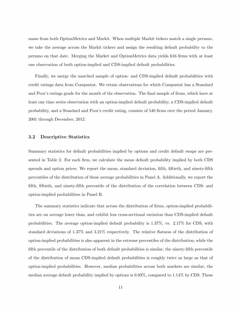
name from both OptionMetrics and Markit. When multiple Markit tickers match a single permno,

we take the average across the Markit tickers and assign the resulting default probability to the

permno on that date. Merging the Market and OptionMetrics data yields 616 firms with at least

one observation of both option-implied and CDS-implied default probabilities.

Finally, we merge the matched sample of option- and CDS-implied default probabilities with

credit ratings data from Compustat. We retain observations for which Compustat has a Standard

and Poor’s ratings grade for the month of the observation. The final sample of firms, which have at

least one time series observation with an option-implied default probability, a CDS-implied default

probability, and a Standard and Poor’s credit rating, consists of 540 firms over the period January,

2001 through December, 2012.

3.2 Descriptive Statistics

Summary statistics for default probabilities implied by options and credit default swaps are pre-

sented in Table 2. For each firm, we calculate the mean default probability implied by both CDS

spreads and option prices. We report the mean, standard deviation, fifth, fiftieth, and ninety-fifth

percentiles of the distribution of these average probabilities in Panel A. Additionally, we report the

fifth, fiftieth, and ninety-fifth percentile of the distribution of the correlation between CDS- and

option-implied probabilities in Panel B.

The summary statistics indicate that across the distribution of firms, option-implied probabili-

ties are on average lower than, and exhibit less cross-sectional variation than CDS-implied default

probabilities. The average option-implied default probability is 1.37%, vs. 2.17% for CDS, with

standard deviations of 1.37% and 3.21% respectively. The relative flatness of the distribution of

option-implied probabilities is also apparent in the extreme percentiles of the distribution; while the

fifth percentile of the distribution of both default probabilities is similar, the ninety-fifth percentile

of the distribution of mean CDS-implied default probabilities is roughly twice as large as that of

option-implied probabilities. However, median probabilities across both markets are similar; the

median average default probability implied by options is 0.93%, compared to 1.14% by CDS. These

11

results suggest a strong skew in the average CDS-implied default probability.

We observe a substantial but imperfect correlation between CDS-implied and option-implied

probabilities. At the median, the default probabilities have a correlation coefficient of 0.59, sug-

gesting that there is some information that is not common between the securities. Even at the 95th

percentile, the correlation is less than 1.0. /footnoteAt the fifth percentile, note that the correla-

tion between the two default probabilities is negative. However, we find that this result is driven

by the large gaps in the time series for some firms, with virtually all of the negative correlations

concentrated in firms with relatively few time series observations.

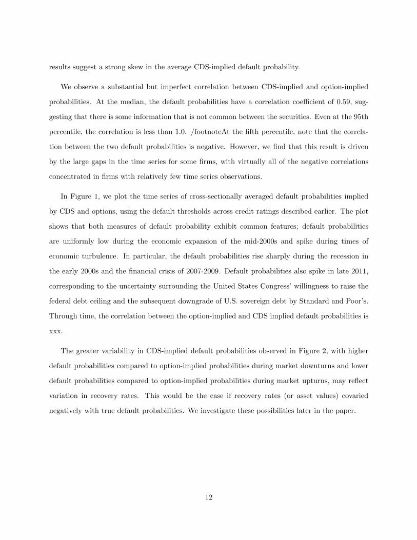
In Figure 1, we plot the time series of cross-sectionally averaged default probabilities implied

by CDS and options, using the default thresholds across credit ratings described earlier. The plot

shows that both measures of default probability exhibit common features; default probabilities

are uniformly low during the economic expansion of the mid-2000s and spike during times of

economic turbulence. In particular, the default probabilities rise sharply during the recession in

the early 2000s and the financial crisis of 2007-2009. Default probabilities also spike in late 2011,

corresponding to the uncertainty surrounding the United States Congress’ willingness to raise the

federal debt ceiling and the subsequent downgrade of U.S. sovereign debt by Standard and Poor’s.

Through time, the correlation between the option-implied and CDS implied default probabilities is

xxx.

The greater variability in CDS-implied default probabilities observed in Figure 2, with higher

default probabilities compared to option-implied probabilities during market downturns and lower

default probabilities compared to option-implied probabilities during market upturns, may reflect

variation in recovery rates. This would be the case if recovery rates (or asset values) covaried

negatively with true default probabilities. We investigate these possibilities later in the paper.

12

3.3 Default Probabilities and Credit Ratings

To investigate cross-sectional variation in implied default probabilities, we first examine summary

statistics for default probabilities by credit rating. Some of the cross-sectional variation is induced,

as we use the historical returns on firms of different credit ratings to guide the level of default

thresholds for option-implied default probabilities. Therefore, we also examine option-implied de-

fault probabilities holding the default threshold fixed.

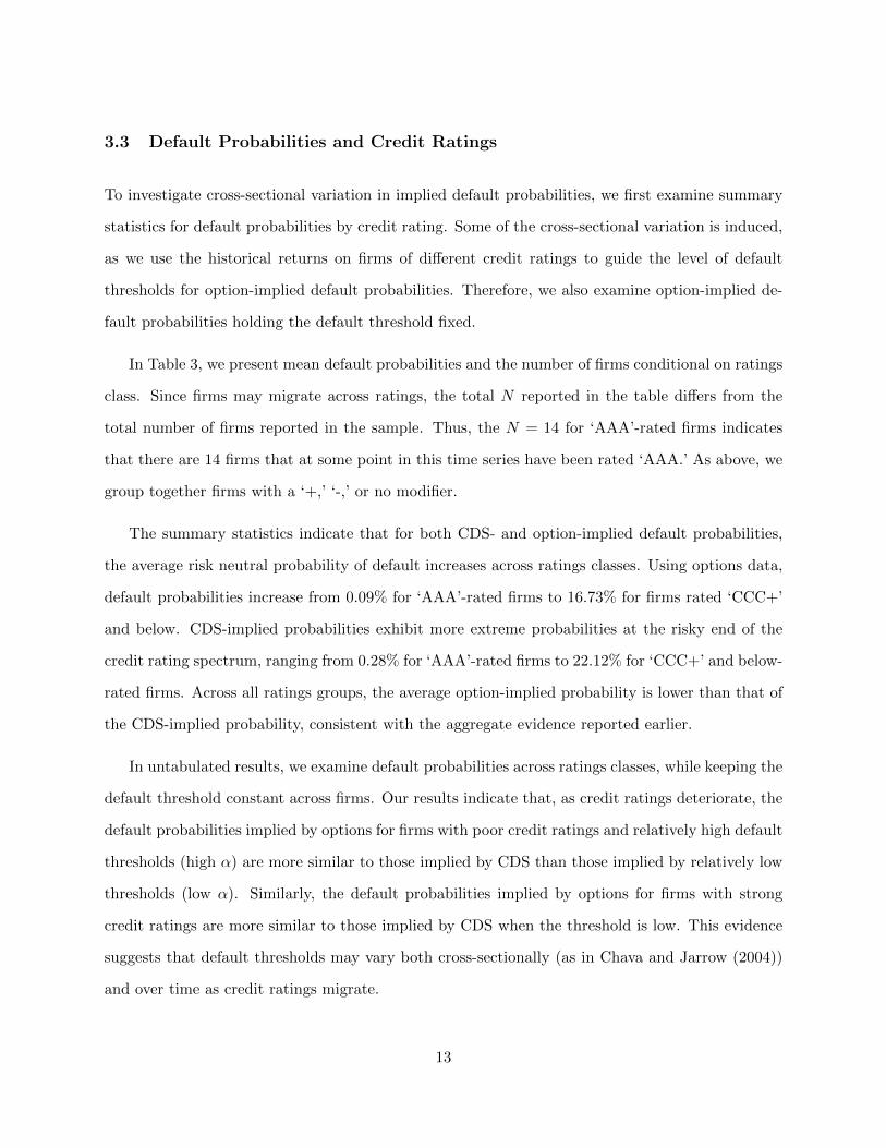
In Table 3, we present mean default probabilities and the number of firms conditional on ratings

class. Since firms may migrate across ratings, the total N reported in the table differs from the

total number of firms reported in the sample. Thus, the N = 14 for ‘AAA’-rated firms indicates

that there are 14 firms that at some point in this time series have been rated ‘AAA.’ As above, we

group together firms with a ‘+,’ ‘-,’ or no modifier.

The summary statistics indicate that for both CDS- and option-implied default probabilities,

the average risk neutral probability of default increases across ratings classes. Using options data,

default probabilities increase from 0.09% for ‘AAA’-rated firms to 16.73% for firms rated ‘CCC+’

and below. CDS-implied probabilities exhibit more extreme probabilities at the risky end of the

credit rating spectrum, ranging from 0.28% for ‘AAA’-rated firms to 22.12% for ‘CCC+’ and below-

rated firms. Across all ratings groups, the average option-implied probability is lower than that of

the CDS-implied probability, consistent with the aggregate evidence reported earlier.

In untabulated results, we examine default probabilities across ratings classes, while keeping the

default threshold constant across firms. Our results indicate that, as credit ratings deteriorate, the

default probabilities implied by options for firms with poor credit ratings and relatively high default

thresholds (high α) are more similar to those implied by CDS than those implied by relatively low

thresholds (low α). Similarly, the default probabilities implied by options for firms with strong

credit ratings are more similar to those implied by CDS when the threshold is low. This evidence

suggests that default thresholds may vary both cross-sectionally (as in Chava and Jarrow (2004))

and over time as credit ratings migrate.

13

3.4 Firm Characteristics and Probability of Default

As shown in the previous section, option-implied risk neutral probabilities of default are strongly and

positively correlated with CDS-implied risk neutral probabilities of default, and are cross-sectionally

correlated with Standard and Poor’s credit ratings. We analyze cross-sectional variation in default

probabilities in more detail in this section, by examining the relation between both estimates of

default probability and firm characteristics. In particular, we use a variant of Campbell, Hilscher,

and Szilagyi (2008), who specify a pooled logit model for prediction of default, yielding estimates

of the physical probability of default. Instead of using a limited dependent variable based on an

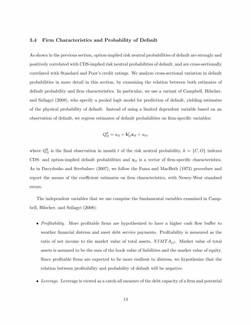
observation of default, we regress estimates of default probabilities on firm-specific variables:

Qkit = ait + b′itxit + uit,

where Qkit is the final observation in month t of the risk neutral probability, k = {C,O} indexes

CDS- and option-implied default probabilities and xit is a vector of firm-specific characteristics.

As in Davydenko and Strebulaev (2007), we follow the Fama and MacBeth (1973) procedure and

report the means of the coefficient estimates on firm characteristics, with Newey-West standard

errors.

The independent variables that we use comprise the fundamental variables examined in Camp-

bell, Hilscher, and Szilagyi (2008):

• Profitability. More profitable firms are hypothesized to have a higher cash flow buffer to

weather financial distress and meet debt service payments. Profitability is measured as the

ratio of net income to the market value of total assets, NIMTAj,t. Market value of total

assets is assumed to be the sum of the book value of liabilities and the market value of equity.

Since profitable firms are expected to be more resilient to distress, we hypothesize that the

relation between profitability and probability of default will be negative.

• Leverage. Leverage is viewed as a catch-all measure of the debt capacity of a firm and potential

14

financial distress. We measure a firm’s leverage as the ratio of total liabilities to the market

value of total assets, as defined above. We expect this variable, TLMTAj,t to be positively

related to probability of default.

• Cash. Campbell, Hilscher, and Szilagyi (2008) hypothesize that cash provides a buffer in the

case of financial distress, as a firm can use its cash reserves to service debt. The variable,

CASHMTAj,t is measured as the ratio of cash and short-term investments to the market

value of total assets. Since cash represents a buffer, we anticipate that the variable will be

negatively related to probability of default. However, it should be noted that the relation

between this variable and default probability is not unambiguous. Acharya, Davydenko, and

Strebulaev (2012) show that credit spreads and cash holdings are positively correlated. The

authors provide evidence to support the notion that riskier firms hold more cash due to a

precautionary savings motive.

• Book-to-Market. Book-to-market is a measure of the growth prospects of the firm, and also

reflects the equity market’s outlook for the future of the company. If equityholders anticipate

bankruptcy, market value of equity is likely to fall, increasing this ratio. We measure the

book-to-market ratio, BMj,t, as the ratio of book value of equity to market value of equity,

where book value of equity is the difference in the book value of assets and book value

of liabilities. If high book-to-market firms are more distressed, we expect the ratio to be

positively associated with probability of default.

• Volatility. A central idea in the Merton (1974) model is that distance to default of firms

with more volatile asset returns, which are in turn reflected in more volatile equity returns,

is smaller. We measure volatility as the annualized standard deviation of the firm’s daily

stock return over the past three months, SIGMAj,t. We expect that firms with more volatile

equity will have a higher probability of default.

• Excess return. The excess return, EXRETj,t, is the quarterly log return on the firm’s equity

in excess of the log return on the S&P 500 index. This variable is expected to be negatively

15

related to the probability of default, as we expect that firms with high probabilities of default

will experience declines in share price in anticipation of default.

• Price. Distressed firms tend to trade at low prices per share. This measure, PRICEj,t is the

minimum of the natural log of the firm’s share price, or the log of $15. Since distressed firms

tend to have low stock prices, we expect a negative relation to default probability.

• Relative size. RSIZEj,t is the log ratio of the capitalization of firm j to that of the CRSP

value-weighted index. Both size and book-to-market are hypothesized to be related to distress

by Fama and French (1992) and we expect a negative relation between this variable and default

probability.

Market data are obtained from CRSP and quarterly firm financial information is obtained from

Compustat. Since we are interested in correlations rather than prediction, we measure firm financial

information concurrently with Compustat data, rather than allowing for a lag as in Campbell,

Hilscher, and Szilagyi (2008). Quarterly information for a firm’s first quarter ending in March is

matched to month-end default probabilities measured from January 1 through March 31 of the

same year.

Summary statistics for the firm-specific variables are shown in Table 4. We present means and

medians for firms in our sample, as well as for firms in the CRSP/Compustat universe not in our

sample. The table shows that on average, our sample firms are more profitable, more levered, have

lower volatility and book-to-market ratios, have larger relative market capitalizations and lower cash

holdings, and are less likely to be low-priced firms. These results are expected, as the requirement

that firms in our sample have CDS written on them tilts us toward larger, more established firms.

The results of the Fama and MacBeth (1973) regressions of default probabilities on the ex-

planatory variables are presented in Table ??. We split the sample into financial and non-financial

firms, defined by the firm’s GICS sector from Compustat. Campbell, Hilscher, and Szilagyi (2008)

consider only non-financial firms, and ratios such as leverage and book-to-market ratio are likely

to be very different for financial firms than non-financial firms.

16

The results for non-financial firms suggest a number of similarities in the correlations between

CDS-implied and option-implied default probabilities. First, implied default probabilities for non-

financial firms are statistically significantly decreasing in profitability, relative size, and price when

default probabilities are measured using either options or CDS. The default probabilities are statis-

tically significantly increasing in leverage and return volatility. All of these relations are consistent

with the predictions above and the results in Campbell, Hilscher, and Szilagyi (2008). The book-to-

market ratio is negatively associated default probabilities, counter to the arguments in Campbell,

Hilscher, and Szilagyi (2008). As we will discuss later, this result may be due to book-to-market

ratios proxying for differences in recovery rates, rather than distress.

We observe one puzzling result: when default probabilities are measured using option prices, a

high excess return is associated with a high default probability.

Results for financial firms are broadly similar to those for non-financial firms, but fewer coef-

ficients are statistically significantly different than zero. The results indicate that for both sets of

security measures, volatility is positively associated with the probability of default, and size and

price are associated with lower probability of default. Book-to-market ratios are positively, but only

marginally significantly associated with default probabilities in the case of CDS. For financial firms,

the option-implied probabilities are negatively and statistically significantly associated with cash

holdings. Finally, in the option-implied measures, excess returns are again positively associated

with probability of default.

In general, the results of this analysis suggest that the relation of firm characteristics to both

CDS and option-implied default probabilities are consistent with the underlying fundamentals of

the firm.

17

4 Sources of Differences Between Option- and CDS-Implied De-

fault Probabilities

In a previous section, we compared the probabilities of default implied by CDS (and a constant

recovery rate) to those obtained from equity options. For the median firm in the cross-section, the

default probabilities are strongly correlated and, when we aggregate default probabilities across

firms, option-implied and CDS-implied default probabilities are very highly correlated. This ev-

idence suggests that the probabilities contain broadly similar information about time series in-

novations in probabilities of default. Additionally, the evidence suggests that credit ratings and

firm characteristics that are hypothesized to be related to the probability of default are related to

both option- and CDS-implied default probabilities. This evidence suggests that both estimates of

default probabilities are capturing cross-sectional information.

However, as noted above, default probabilities estimated from the CDS and equity options

market are not perfectly correlated. In particular, CDS-implied default probabilities have higher

cross-sectional variation and higher skew. It is possible that these differences may simply arise from

estimation error; in particular, the option-implied default probabilities are based on estimation of

risk neutral moments and the imposition of the NIG distributional assumption. In this section, we

consider some systematic, rather than measurement-related reasons that the probabilities from the

two markets might differ.

One possibility mentioned above is that differences in option and CDS prices are due to variation

in rates of recovery. Studies of recovery rates, including Altman and Kishore (1996) and Altman

(2011) suggest that recovery rates vary cross-sectionally and over time. Cross-sectional variation

associated with recovery rates may also drive some differences in the Fama and MacBeth (1973)

regressions of CDS- and option-implied default probabilities on firm characteristics above.

A second possibility is that aggregate and security-level liquidity may impact option and CDS

prices, and therefore the imputed default probabilities derived from these markets. For example, our

option-based probabilities begin by calculating implied volatility surfaces using out-of-the-money

18

puts and calls. These contracts, especially deep out-of-the-money contracts, are likely to have less

liquidity than near-the-money puts and calls. Further, we are interpolating the volatility surface at

a maturity of 365 days, where there are likely to be fewer available contracts with lower liquidity.

CDS are also likely to suffer from liquidity issues. We are using one-year CDS contracts, which

have lower liquidity than five-year contracts. Finally, CDS are relatively sparsely traded at the

beginning of our sample period and also suffered from liquidity issues during the financial crisis.

A third possibility involves the default threshold, α, that is used when estimating default prob-

abilities from the options market. That is, higher α’s may result in option-implied default probabil-

ities that better match CDS-implied default probabilities in times when CDS-implied probabilities

are high and for firms with poorer credit ratings. Thus, it may be that the market perceives the

default threshold for equity as being different during times of financial market stress or when a

firm is closer to its default boundary. There may be other economic rationales for a varying de-

fault threshold, such as strategic bankruptcies; that is, in some circumstances, firms may find it

beneficial to default even if they are solvent and able to make debt payments.

To analyze the differences in the information about default probability in the two markets, we

begin with the relation between the CDS spread, the default probability, and the recovery rate (or

loss given default). If we consider a simple one-period CDS contract:

St = QCt (1−Rt) ,

the CDS spread is the product of the default probability and the loss given default, or one minus

the recovery rate. In logs, the log spread is the sum of the log of default probability and log of

one minus the recovery rate. While the relationship between spreads, default probabilities, and

recovery rates is not strictly log-linear as shown in equation (3), this approximation is useful for

understanding the intuitive relation between spreads, default probabilities and recovery rates.

Under standard practice of assuming a constant recovery rate of 40%, the log spread and the

log CDS implied default probability in this simple model are perfectly correlated by construction,

19

both cross-sectionally and in the time series. However, if the option-implied default probability

is a valid estimate of the true default probability, then subtracting the log option-implied default

probability from the log CDS spread should provide an (approximate) estimate of log loss given

default, that is allowed to vary across firms and through time. Of course, this difference will also

capture effects related to liquidity, mis-specification of the default threshold, and other estimation

errors. We calculate this difference, D, and consider its properties below.

4.1 Cross-market inferences

In Table 6, we report the average difference in the log spread and the log option-implied default

probability, denoted as D, in the first column, for three constant threshold values of α and for a

threshold value that varies across firms according to credit rating. In the remaining columns, we

mirror our results for default probabilities and also present the standard deviation, fifth percentile,

fiftieth percentile, and 95th percentile of the cross-sectional distribution of D. In Panel B, we

compute correlations in the log difference D for each firm when the critical threshold is 0.05, 0.10,

and 0.15 and when the critical threshold varies across credit rating as described earlier in the paper.

Again, we present fifth, fiftieth, and ninety-fifth percentiles of the cross-sectional distribution of

these correlations.

In Panel A of Table 6, the results show that with α = 0.05, the mean and median of D are

positive. Without controlling for liquidity effects, estimation error, etc., this would imply negative

recovery rates, or losses given default in excess of 100%. Intuitively, these negative recovery rates

are related to the low default probabilities obtained when using a default threshold of 0.05 for

all firms. As can be seen in the equation above, holding the CDS value constant, as the default

probability declines, the recovery rate must also decline. The option-implied default probabilities at

a default threshold of 0.05 are sufficiently low that using them to impute recovery rates calculated

from observed CDS spreads forces those rates below zero. This result is more likely to hold for

firms with low credit ratings.

This result is also consistent with our interpretation of the evidence in Table 1 and Figure

20

1. At higher default thresholds, option-implied default probabilities increase and so average and

median values of D decline. At α = 0.10, the mean (median) D is equal to -0.65 (-0.71). Without

controlling for other effects, this value of D implies a recovery rate of 48 (51%)

When the threshold is set by credit ratings, xxx

The results in Panel B of Table 6 indicate that log differences in spreads and option-implied

default probabilities across critical thresholds are also highly correlated. The fifth percentile cor-

relation in estimates of D between default thresholds of 0.05 and 0.15 is 0.94, which is the lowest

correlation observed. The median correlation observed when α = 0.05 and α = 0.15 is close to

perfect, with a coefficient of 99%; the ninety-fifth percentile correlation of estimates of D across

firms is perfect. Our interpretation is that, although the level of the log differences varies across

default thresholds, estimates across critical values contain very similar information about relative

values of D in the cross-section.

In Figure 2, we present the time series of average estimates of D across firms for different default

thresholds. It is apparent that the time series are highly correlated. The behavior of D through

time is consistent with the interpretation that it is inversely related to loss given default, or one

minus the recovery rate; that is, note that regardless of the default threshold the average D varies

strongly with business conditions, consistent with the relation between recovery rates and market

fundamentals documented in Jankowitsch, Nagler, and Subrahmanyam (2014). In particular, the

variation in D implies that recovery rates are low in the early 2000s and recover with the economy

in the mid-2000s. The rates plunge during the financial crisis of 2007-2009, and then gradually rise.

The secondary decrease in recovery rates in 2011 is contemporaneous with the downgrade of U.S.

debt in 2011.

Although the time-series variation in D is quite similar across default thresholds, and the

variation through time for all thresholds seems sensible given market fundamentals, it is clear from

Figure 2 that any inference about the level of implied recovery rate is sensitive to the level of the

default threshold that one chooses. That is, average values of D in the sample are largely positive

for α = 0.05, and frequently positive for α = 0.10. For the default threshold of 0.15, average values

21

of D are almost invariably negative, consistent with average recovery rates that are positive. When

default thresholds vary by firm across credit ratings, xxx

The evidence in Figure 2 that D varies with economic conditions is consistent with an inference

that D contains information about recovery rates, and indicates that the assumption that recovery

rates are constant through time is a poor fit to the data. In the next sections, we examine the

variation in D across sectors, and analyze the relation between spreads and option-implied default

probability estimates, while controlling for other factors such as liquidity.

Recovery Rates and Industry Sectors

Altman and Kishore (1996) report considerable variation in realized recovery rates by three-digit

SIC code. In this section, we analyze variation in D across sectors. Since the results in Figure 2

indicate that setting a constant α = 0.15 results in estimates of D that are consistent with positive

recovery rates, and the time-series information in D across different values of α is very similar,

we report results using only 2 values of D: one that uses a constant default threshold α = 0.15

across all firms, and a second that uses a firm-specific default threshold based on credit rating. We

utilize the GICS sector definitions, which separate firms into 10 sectors; Energy, (EN) Materials

(MA), Industrials (IN), Consumer Discretionary (CD), Consumer Staples (CS), Healthcare (HC),

Financial (FI), Information Technology (IT), Telecommunications (TC), and Utilities (UT). Sector

classifications are obtained from Compustat.

We present summary statistics for D in Table ??. Specifically, each week we calculate the

average difference (by sector) of the implied one-year CDS spreads and option-implied default

probabilities. The average number of firms in each sector varies from 5 (Telecommunications) to 51

(Discretionary). Grouped into sectors, inferences about D are much more precise. With a default

threshold of α = 0.15, the average D is negative for each of the ten sectors, and varies from -1.14

to -1.79. For nine out of the ten sectors, the maximum value of D is also negative. In addition,

the standard deviation of D is smaller by a factor of 2 than the dispersion in D across individual

firms reported in Table 4. When default thresholds are allowed to vary across firms based on credit

ratings, xxx

22

We observe considerable variation in D across sectors. At the constant threshold of /alpha =

0.15, the lowest values of D (of -1.79 in both cases) are observed in Staples and Healthcare, corre-

sponding to higher implied recovery rates; the highest values of D (-1.14 and -1.19) are observed

in Consumer Discretionary and Utilities, respectively. The result that average values of D are

higher, and thus recovery rates are lower, for Utilities is surprising, particularly given the evidence

in Altman and Kishore (1996), who find that the highest average recovery rates in their sample

is observed in public utilities. Note, however, that we also observe the second highest time-series

variability in D in Utilities (and the highest variability in D is observed in the financial sector).

This suggests that inferences about recovery values in the Utilities sector may be sensitive to the

sample period that one uses. In general, the values of D reported in Table 5 are consistent with

positive recovery rates. Ignoring liquidity effects, biases and estimation error, the recovery rates

implied by the average values of D in Table 5 vary from 68% (in Consumer Discretionary) to 83%

(in Healthcare and Staples).

We examine time-series variation in sector averages of D, in Figure 4, where we show the weekly

cross-sectional average value of D in each sector. We observe significant time-series variation in D

in every sector, and the values of D in each sector generally share features in common with the

aggregate time series plot in Figure 3. That is, implied recovery rates are generally low during the

economic contraction of the early 2000s, rise in the mid-2000s, and fall sharply with the financial

crisis of 2007-2009. Values of D are negative through the entire sample period for every sector

except Utilities, where we observe positive values of D in 2003 and again in the fall of 2008 and

early 2009.

Although there are similarities in the time-series, there do appear to be differences in the sen-

sitivity of sectors to fundamentals. For example, Healthcare, Telecommunications and Information

Technology, while clearly affected by economic conditions, show relatively small declines in D (and

so relatively small implied increases in recovery rates) during the mid-2000s expansion and rela-

tively smaller decreases in implied recovery rates during the crisis. Financial firms experience very

sharp changes in D through the sample period; the large decline in D in the mid-2000s implies a

23

large increase in recovery rates at that time, followed by a very large reversal in D, and so implied

recovery rates, at the time of the financial crisis. Energy, Materials, Consumer Discretionary, and

Utilities also seem to be severely impacted by economic conditions.

Broadly, this variation across sectors seems sensible. When economic conditions weaken, the

value of factors to production, such as energy and materials falls, and with it the values of these

assets. Similarly, the value of consumer discretionary assets is likely to be significantly affected by

economic conditions. In contrast, the value of healthcare and technology firm assets may be less

subject to variation in the economy. The biggest surprise for us is utilities; we would expect the

value of these assets to be less sensitive to economic conditions, but the sector shows surprising

weakness in 2003 and again during the financial crisis.

Firm Characteristics and Implied Recovery

We undertake a more detailed examination of the cross-sectional variation in D by repeating

the Fama and MacBeth (1973) analysis undertaken in Section 3.4 above, with D replacing the

implied default probability as the dependent variable. Results of these regressions are presented in

Table 7.

The regression results for the “non-strategic variables” are quite similar to those in the CDS-

implied default probability regressions in Table 5. D is negatively related to profitability, relative

size, cash holdings and, in some specifications, to price. The difference is positively related to

leverage and equity volatility. Generally, these results are consistent with the idea that the higher

the value of assets available to debtholders in case of a bankruptcy, the higher the rate of recovery

that investors can expect on their debt. Thus, these variables broadly support the interpretation

of D as potential loss given default.

Variables that Davydenko and Strebulaev (2007) relate to costs of liquidation are generally

statistically significantly related to the difference in spread and option-implied probability, D,

with the exception of the book-to-market ratio, which is only marginally significant. The three

statistically significant measures are all negatively related to D. In the case of non-fixed assets and

24

R&D expenditures, this sign is the opposite of that found in the Alderson and Betker (1996) study

of liquidation costs in Chapter 7. However, these results may not be as applicable in a Chapter 11

context, and the negative sign on TANG, and its likely correlation with NONFIXED suggests

that firms with more tangible assets are more likely to have higher differences in log credit default

spreads and option-implied default probabilities. This evidence appears consistent with the idea

that firms with a greater fraction of tangible assets are expected to have greater rates of recovery

in case of a debt default.

Finally, the strategic variables INST and NSHARE also exhibit behavior similar to the results

reported in Table 5 for option-implied default probabilities. INST is not statistically significantly

associated with differences across firms in D, suggesting that although it is positively associated

with option-implied default probabilities, institutional ownership does not statistically significantly

affect ex ante beliefs about recovery. This result is again consistent with the idea that INST

captures the likelihood of strategic default. The number of shareholders, NSHARE, is statistically

significantly negatively associated with loss given default. Again, Davydenko and Strebulaev (2007)

use this variable to capture renegotiation frictions, specifically the degree of difficulty in coordination

across shareholders in bankruptcy negotiation. The results suggest that the more difficult this

coordination, the lower D imply that, if D measures loss given default, the expectation of loss

given default is lower the more difficult it is for shareholders to coordinate.

We view these results as broadly supporting the interpretation of D as a measure of the loss

given default. It is particularly interesting to us to note areas in which the results from Table

7 differ from those for option-implied probabilities in Table ??. Cash holdings and stock price

appear to be at least marginally significantly related to D, but not to the option-implied default

probability. These results suggest to us that these variables are more potentially relevant to recovery

in default than the probability that a firm will default. This idea is reinforced by the opposing

signs for NONFIXED and TANG in the regressions of D on firm characteristics compared to

option-implied default probabilities. The results indicate that firms with more cash, more tangible

assets, and more non-fixed assets may be more likely to default but, to the extent that D measures

25

loss given default, will have a greater surplus of assets to satisfy bondholders claims.

4.2 Liquidity and Default Probabilities

While variation in recovery rates is an appealing explanation for differences in risk neutral default

probabilities across options and CDS, an additional possibility is that these probabilities differ as

a result of frictions. In particular, the out-of-the-money options used to construct the moments

that are used as inputs into the option-implied default probabilities may be thinly traded. Further,

the liquidity of CDS contracts is low in the early part of our sample period, and, for some firms

in our sample, is low again during the financial crisis. Since the data suggest a marked decline in

implied recovery associated with the crisis, it is possible that this reflects not variation in ex ante

recovery, but rather a decline in market liquidity. 6 As a consequence, we estimate the relation

between changes in the (log) spread and changes in the log of option-implied default probabilities,

while controlling for liquidity effects.

Illiquidity in the CDS and options markets may reflect both security-specific and market-wide

variation in liquidity.7 We are somewhat limited in measuring security-specific liquidity by the

fact that we have information only on quotes, and not on trades, for both sets of securities. In

the case of options, we have information on bid-ask spreads, open interest, and volume. Since the

default probabilities recovered from options are likely to depend most on the prices of out-of-the-

money options close to 365 days to maturity, we construct SPREADOt , the average percentage

bid-ask spread for the out-of-the-money options used in constructing our volatility surface. We also

compute V OLOt and OPENOt , the sum of volume and open interest for these contracts. In the case

of CDS, we have a measure of the depth for five-year CDS contracts. We assume that depth for

the one-year contracts is correlated with the depth of the five-year contracts, and use DEPTHCt ,

the depth of the five-year contract, as another measure of liquidity.

6It is possible that precipitous declines in market liquidity are associated with declines in asset values and thusrecovery rates (see, e.g., Brunnermeier and Pedersen (2009). If that is the case, our controls for market liquidity willcause the decline in recovery rates during periods of market illiquidity to be estimated conservatively.

7Note that by examining Fama and MacBeth (1973) regressions we are in effect including a time fixed effect in theregression. Thus, the results reported earlier supporting the interpretation of D as a loss given default are unlikelyto be due to aggregate liquidity effects.

26

To capture aggregate liquidity, we use two measures that may be of particular importance in

the fixed income security markets. First, we use the Treasury-Eurodollar spread, TEDt, measured

as the difference in 90-day LIBOR and 90-day Treasury Bill yields. An increase in the TED spread

potentially indicates an increase in interbank counterparty credit risk, and a consequent drop in

financial liquidity. The second measure is the root mean squared error of the difference in market

Treasury security yields from those implied by a Nelson-Siegel-Svensson model. This measure,

NOISEt, is investigated in Hu, Pan, and Wang (2013). The authors suggest that NOISEt is high

when there is less arbitrage capital available in the Treasury market, a condition associated with

lower liquidity. Finally, we include a proxy for liquidity in the equity markets; Nagel (2012) suggests

that a high level of the VIX index, V IXt is associated with a high risk premium, and a consequent

large reduction in liquidity provision, in equity markets. The TED spread is constructed using data

from the Federal Reserve and NOISEt is obtained from Jun Pan’s webpage.8 Data on the VIX

are also obtained from the Federal Reserve.

We plot natural logs of these liquidity series in Figure ??. Given their construction, note that,

with the exceptions of volume, open interest and depth measures, an increase in these measures

represents a decrease in liquidity. The aggregate series exhibit a familiar pattern, dominated by a

sharp decrease in liquidity associated with the financial crisis of 2007-2009. This decline in measures

of aggregate liquidity is associated with an increase in counterparty credit risk and a decrease in

the arbitrage capital available in the fixed income and equity markets. The trend in these series

is strongly related to the trend in the implied recovery rates in Figure 3. In particular, the log

recovery rate is -83% correlated with log NOISEt and -80% correlated with the log of the VIX.

These trends also induce in-sample nonstationarity of the series.

The option-specific liquidity measures exhibit different patterns. These series are the cross-

sectional averages each week of the individual firm data used in our analysis. Volume and open

interest are generally increasing over the sample period. There is some periodicity in these series

associated with option writing dates; open interest and volume decline as options approach maturity.

8We thank Jun Pan for making these data available at http://www.mit.edu/~junpan/.

27

There is a sharp downward spike in open interest in option markets associated with the financial

crisis, and a less striking downward spike in volume. Additionally, the spread shows a sharp upward

spike during the crisis. There is some relation of these measures with the aggregate series; however,

none of the option-specific series exhibit more than 40% correlation with the aggregate liquidity

measures.

Finally, the depth of the five-year CDS contract does exhibit a strong time trend. Contract

depth steadily increases from 2001 to 2005, before slackening slightly in 2006 through 2007. CDS

contract depth plummets in early 2008 until mid-2009, clearly associated with the financial crisis.

Depth remains low in 2010 and 2011, before picking up somewhat in 2012.

Given the strong trends in these data, we estimate the relation between first differences in the

CDS spread and differences in the liquidity variables and differences in the option-implied default

probability, beginning at the aggregate level. That is, we estimate the parameters of a regression,

∆sa,t = aa + ba,1/DeltaQoa,t + ba,2∆tedt + ba,3∆noiset + ba,4∆vixt + ba,5∆spreadOa,t

+ba,6∆volOa,t + ba,7∆openOa,t + ba,8∆depthCa,t + ea,t, (10)

where a indicates that we are measuring the quantity at the aggregate level, where aggregate vari-

ables are calculated as the cross-sectional average of individual time series observations. Lowercase

variables are natural logs of their uppercase counterparts.

Results of this regression are reported in Table 8. The results suggest that innovations in

fixed income market liquidity variables are not statistically significantly associated with innova-

tions in CDS spreads. An increase in counterparty credit risk as measured by the TED spread is

positively, but not significantly associated with increases in spreads, while a decrease in arbitrage

capital in fixed income markets, measured by a positive innovation in NOISEt, is negatively, but

insignificantly associated with innovations in CDS spreads. In contrast, an innovation in the VIX is

associated with a significant increase in CDS spreads, suggesting that some of the marked decline in

recovery rates exhibited over the course of the financial crisis may be associated with an increase in

28

market-wide volatility. This result may be consistent with the evidence in Nagel (2012), who shows

that an increase in the VIX is associated with a reduction of equity arbitrage capital; alternatively,

rather than a liquidity narrative, the increase in market-wide volatility may be associated with an

increase in aggregate risk which then causes a decline in asset values and so an increase in CDS

spreads.

There is weak evidence that security-specific liquidity is related to CDS spreads. Specifically,

innovations in the open interest of options are statistically significantly positively associated with

innovations in CDS spreads. Thus, as options become less liquid, reflected in lower open interest,

this is associated with increases in CDS spreads. This may reflect an aggregate decline in liquidity

in derivatives markets. Again, this result suggests that at least part of the sharp decline in implied

recovery rates during the financial crisis of 2007-2009 may be associated with a decline in liquidity.

Even after controlling for liquidity variables, however, note that the coefficient on differences

in the option-implied default probability is significantly positive and, at 0.961, is not significantly

different from 1. In addition, the R-squared of this regression is relatively large, at 38%. This

evidence suggests that there are significant linkages between the CDS and equity options market;

in particular, changes in the default probabilities inferred from equity options have significant

explanatory power for variation in the prices of CDS.

We also report the results of this regression across sectors in Table 9. The results are generally

consistent with the results observed in the aggregate: we continue to find evidence that changes in

the VIX are positively associated with changes in the average log CDS spread in the sector, and

the coefficient on log changes in the option-implied default probability are very significantly related

to changes in the log CDS spread. In only two sectors, Industrials and Consumer Staples, is the

coefficient on changes in the option-implied default probability significantly different from 1; for

Industrials, the coefficient is significantly larger than 1, at 1.543, and for Consumer Staples, the

coefficient is significantly smaller, at 0.434.

Overall, these results suggest that variation in default probabilities inferred from the option

market is related to variation in the CDS spread; however, there is also evidence that variables

29

such as the VIX and option open interest may influence the relation between CDS spreads and

option-implied default probabilities. As a result, the simple difference between the CDS spread

and option-implied default probability will contain confounding information about liquidity, in

addition to information about recovery rates. In the next section, we examine variation in CDS

spreads after removing information about default probabilities (taken from options markets) and

liquidity effects.

4.3 Inferred recovery rates

In our last analysis, we use the regression above to generate an inferred recovery rate from the

CDS spread, which controls for variation in default probabilities and liquidity effects. Specifically,

we compute an estimate of the residual change in the CDS spread, after removing the effects of

changes in option-implied default probabilities as well as liquidity effects.

rt = aa +

t∑j=0

ea,t−j ,

Since the regression equation is in differences, note that we are calculating cumulated values of the

changes in CDS spreads that are unrelated to changes in option-implied default probabilities and

liquidity variables.

In Figure ??, we plot this variable, which is an estimate of the cumulative percentage increase

or decrease in recovery rates relative to a. The figure shows that, even after controlling for liquidity,

the pattern in implied recovery rates is strikingly similar to the variation in D in Figure 2. Implied

recovery rates drop by 20% in the early 2000s recession, before a large increase in the mid-2000s.

Recovery rates plunge during the financial crisis, before slowly recovering to pre-crisis levels by the

end of the sample period.

Overall, these results indicate that, after controlling for liquidity effects and changes in default

probabilities, the recovery rates inferred from CDS exhibit significant time-series variation. Specifi-

cally, implied recovery rates exhibit substantial increases prior to the financial crisis, decline sharply

30

during the crisis, and then recover by the end of 2013.

5 Conclusion

In this paper, we propose a new method of estimating default probabilities for firms. Using option

prices, we construct an estimate of the risk-neutral density; the default probability for the firm is the

mass under the density up to the return that corresponds to a default event. We estimate default

probabilities for three different default thresholds; we find that, although the level of estimated

default probabilities is sensitive to the choice of default threshold, they are very highly correlated

with one another and behave very similarly over time.

We examine the relationship of the option-implied default probabilities to default probabilities

estimated from CDS prices, as well as their relation to firm characteristics, and ratings categories.

We find that option-implied are strongly, but not perfectly, related to CDS default probabilities that

assume constant recovery rates, with the latter exhibiting higher variation and higher skewness.

With respect to firm characteristics and ratings categories, the option-implied default probabilities

behave one would expect. Specifically, the default probabilities increase as ratings decline; in

addition, default probabilities are significantly and positively related to leverage, volatility and

book-to-market equity ratio; they are negatively and significantly related to profitability, past

quarterly excess returns, size and price. The one surprising result is that we find that estimated

default probabilities increase with cash holdings.

If option-implied default probabilities are valid, then an examination of the relation between

these probabilities and CDS prices should provide information about recovery rates. We examine

the log difference in spreads and option-implied default probabilities, and find significant time-series

variation in this difference, which is related to economic conditions. While the difference is highly

correlated across default thresholds, the evidence indicates that default thresholds as low as 5% are

too low, in that they appear to be consistent with negative recovery rates. We also find evidence

of significant cross-sectional variation in this difference.

31

When we estimate the relation between CDS spreads and option-implied default probabilities,

while controlling for liquidity effects, we find evidence that the VIX and option open interest are

significantly and positively related to CDS spreads. In addition, in aggregate, and for eight out of

the ten sectors that we analyze, we cannot reject the hypothesis that the coefficient on the option-

implied default probability is equal to one. Finally, after controlling for changes in the default

probability (taken from the options market) and liquidity effects, the recovery rate inferred from

CDS prices again shows a strong relation to underlying business conditions. Overall, the equity

option market may provide useful information with which to infer default probabilities, as well as

the recovery values of underlying assets.

32

Appendix

The scale-invariant NIG distribution is characterized by the density function

f (x;α, β, µ, δ) =α

πδexp

(√α2 − β2 − βµ

δ

) K1

(α

√1 +

(x−µδ

)2)√

1 +(x−µ

δ

)2 exp

(β

δx

). (11)

In this expression, x ∈ <, α > 0, δ > 0, µ ∈ <, 0 < |β| < α, and K1 (·) is the modified Bessel

function of the third kind with index 1. The formal properties of the distribution are discussed in

greater detail in Eriksson, Forsberg, and Ghysels (2004). As shown, the density is characterized by

the four parameters α, β, µ, and δ.

As discussed above, a principal advantage of this density function is that it is completely

characterized by its first four moments. More specifically, let the mean, variance, skewness, and

excess kurtosis be denoted as M, V, S, and K. The parameters are nonlinearly related to the

moments by

α =3(4ρ−1 + 1

)K√

(1− ρ−1)(12)

β = sign (S)3(4ρ−1 + 1

)K−1√ρ− 1

(13)

µ = M− sign (S)

√3 (4ρ−1 + 1)V

Kρ(14)

δ =

√3 (4ρ−1 + 1) (1− ρ−1)V

K(15)

where ρ = 3KS−2 − 4 > 1 and sign (·) is the sign function. Thus, given risk neutral moments, one

can compute the risk neutral density.

33

References

Acharya, Viral, Sergei A Davydenko, and Ilya A Strebulaev, 2012, Cash holdings and credit risk,

Review of Financial Studies 25, 3572–3609.

Alderson, Michael J, and Brian L Betker, 1996, Liquidation costs and accounting data, Financial

Management 25, 25–36.

Almeida, Heitor, and Murillo Campello, 2007, Financial constraints, asset tangibility, and corporate

investment, Review of Financial Studies 20, 1429–1460.

Altman, Edward, B Bradi, A Resti, and A Sironi, 2005, The link between default and recovery

rates: Theory, empirical evidence and implications, Journal of Business 78, 2203–2228.

Altman, Edward I., 2011, Default recovery rates and lgd in credit risk modeling and practice, in

Alexander Lipton, and Andrew Rennie, ed.: The Oxford Handbook of Credit Derivatives (Oxford

University Press: Oxford, UK).

Altman, Edward I, and Vellore Kishore, 1996, Almost everything you wanted to know about re-

coveries on defaulted bonds, Financial Analysts Journal 52, 57–64.

Augustin, Patrick, Marti G. Subrahmanyam, Dragon Yongjun Tang, and Sarah Qian Wang, 2016,

Credit default swaps: Past, present, and future, forthcoming, Annual Review of Financial Eco-

nomics.

Bakshi, Gurdip, N Kapadia, and Dilip Madan, 2003, Stock return characteristics, skew laws and

the differential pricing of individual equity options, Review of Financial Studies 16, 101–143.

Bakshi, Gurdip, Dilip Madan, and Frank Zhang, 2006, Understanding the role of recovery in

default risk models: Empirical comparisons and implied recovery rates, unpublished manuscript,

University of Maryland.

Breeden, Douglas, and Robert Litzenberger, 1978, Prices of state contingent claims implicit in

options prices, Journal of Business 51, 621–651.

34

Brunnermeier, Markus K, and Lasse Heje Pedersen, 2009, Market liquidity and funding liquidity,

Review of Financial Studies 22, 2201–2238.

Campbell, John Y, Jens Hilscher, and Jan Szilagyi, 2008, In search of distress risk, Journal of

Finance 63, 2899–2939.

Capuano, Christian, 2008, The option-ipod: the probability of default implied by option prices

based on entropy, IMF Working Paper 08-194.

Carr, Peter, and Liuren Wu, 2011, Simple robust linkages between american puts and credit pro-

tection, Review of Financial Studies 24, 473–505.

Chang, Bo Young, Peter Christoffersen, and Kris Jacobs, 2013, Market skewness risk and the

cross-section of stock returns, Journal of Financial Economics 107, 46–68.

Chava, Sudheer, and Robert Jarrow, 2004, Bankruptcy prediction with industry effects, Review of

Finance 8, 537–569.

Das, Sanjiv, and R Sundaram, 2003, Defaultable equity, option prices and credit-risk measurement:

A separable approach, unpublished manuscript, New York University.

Davydenko, Sergei A., and Ilya A. Strebulaev, 2007, Strategic actions and credit spreads: An

empirical investigation, Journal of Finance 62, 2633–2671.

Dennis, Patrick, and Stuart Mayhew, 2002, Risk-neutral skewness: Evidence from stock options,

Journal of Financial and Quantitative Analysis 37, 471–493.

Doshi, Hitesh, Redouane Elkamhi, and Chayawat Ornthanalai, 2014, The term structure of ex-

pected recovery rates, unpublished manuscript, University of Houston and University of Toronto.

Duffie, Darrell, and Kenneth J Singleton, 1999, Modeling term structures of defaultable bonds,

Review of Financial Studies 12, 687–720.

Eriksson, A, Eric Ghysels, and F Wang, 2009, The normal inverse gaussian distribution and the

pricing of derivatives, Journal of Derivatives 16, 23–37.

35

Fama, Eugene F., and Kenneth R. French, 1992, The cross-section of expected stock returns,

Journal of Finance 47, 427–465.

Fama, Eugene F., and James D. MacBeth, 1973, Risk, return, and equilibrium: Empirical tests,

Journal of Political Economy 81, 607–636.

Hansis, Alexandra, Christian Schlag, and Grigory Vilkov, 2010, The dynamics of risk-neutral im-

plied moments: Evidence from individual options, unpublished manuscript, Goethe University

Frankfurt.

Houweling, Patrick, and Ton Vorst, 2005, Pricing default swaps: Empirical evidence, Journal of

International Money and Finance 24, 1200–1225.

Hu, Xing, Jun Pan, and Jiang Wang, 2013, Noise as information for illiquidity, Journal of Finance

68, 2341–2382.

Jankowitsch, Rainer, Florian Nagler, and Marti G Subrahmanyam, 2014, The determinants of

recovery rates in the u.s. corporate bond market, Journal of Financial Economics 114, 155–177.

Le, Anh, 2007, Separating the components of default risk: A derivate-based approach, Working

Paper, Stern School, New York University.

Madan, Dilip, and Haluk Unal, 1998, Pricing the risks of default, Review of Derivatives Research

2, 121–160.

, and Levent Guntay, 2003, Pricing the risk of recovery in default with absolute priority

rule violation, Journal of Banking and Finance 27, 1001–1025.

Merton, Robert C, 1974, On the pricing of corporate debt: The risk structure of interest rates,

Journal of Finance 29, 449–470.

Nagel, Stefan, 2012, Evaporating liquidity, Review of Financial Studies 25, 2005–2039.

Nelson, Charles R., and Andrew F. Siegel, 1987, Parsimonious modeling of yield curves, Journal of

Business 60, 473–489.

36

O’Kane, Dominic, and Stuart Turnbull, 2003, Valuation of credit default swaps, Lehman Brothers

Fixed Income Quantitative Research Quarterly pp. 1–18.

Pan, Jun, and Kenneth Singleton, 2008, Default and recovery implicit in the term structure of

sovereign CDS spreads, Journal of Finance 63, 2345–2384.

Scheurmann, Til, 2004, What do we know about loss given default?, Wharton Financial Institutions

Center Working Paper No. 04-01.

Stulz, Rene, 2010, Credit default swaps and the credit crisis, Journal of Economic Perspectives 24,

73–92.

Svensson, Lars E. O., 1994, Estimating and interpreting forward interest rates: Sweden 1992-1994,

NBER Working Paper 4871.

Vilsmeier, Johannes, 2011, Updating the option implied probability of default methodology, unpub-

lished manuscript, University of Regensburg working papers in Business Economics and Man-

agement Information Systems.

37

Table 1: Drop in Equity Prices Over 12 Months Prior to Bankruptcy

This table presents the magnitude of the drop in equity prices for firms that file bankruptcy over the 12months. B ankruptcy filing dates are from the updated version of the data in Chava and Jarrow (2004) andare merged with CRSP data on equity prices and returns. We include only those firms that have CRSPdata 12 months prior to the bankruptcy and in the month of bankruptcy filing and whose price declinedover the 12 months prior to filing. The table presents summary statistics by credit rating for the decline inprice by Standard and Poors credit rating for those firms for which ratings data are available. We presentmeans, standard deviations, minima, and maxima of the ratio of the value of the stock price in the monthof bankruptcy filing or delisting price to the price 12 months prior.

Rating N Mean Std. Min. Max.A 3 0.14 0.18 0.00 0.35BBB 26 0.08 0.11 0.00 0.47BB 67 0.13 0.20 0.00 0.98B 197 0.12 0.16 0.00 0.95CCC 59 0.20 0.22 0.00 0.84CC 9 0.45 0.23 0.18 0.86D 22 0.38 0.30 0.02 1.00

38

Table 2: Summary Statistics for Probabilities of Default

Table 2 presents summary statistics for risk neutral probabilities of default implied by credit default swap(CDS) spreads and prices of options on the equity of the same firm. CDS-implied default probabilities arecalculated using a Nelson-Siegel-Svensson zero coupon term structure and constant one-year maturity CDS,assuming a recovery rate of 40% on the underlying bond. Option-implied default probabilities are measuredusing the Bakshi, Kapadia, and Madan (2003) (BKM) procedure for computing risk neutral moments, thencomputing risk neutral probabilities of the Normal Inverse Gaussian distribution (NIG) on the basis of thesemoments. Risk neutral moments are computed using the implied volatility surface of options with 365 daysto maturity. In Panel A, we present means, standard deviations, fifth, fiftieth, and ninety-fifth percentiles ofthe distribution of averages of probabilities implied by each security. In Panel B we present the fifth, fiftieth,and ninety-fifth percentile of the distribution of correlations of a firm’s option-implied and CDS-implieddefault probability. CDS data are from Markit and options data are from OptionMetrics. Data are sampledat the weekly frequency for 539 firms over the period January, 2001 through December, 2012.

Panel A: Distribution

Mean Std p5 p50 p95Option 1.37 1.37 0.24 0.93 4.28

CDS 2.17 3.21 0.24 1.14 8.19

Panel B: Correlations

p5 p50 p95-0.30 0.59 0.91

39

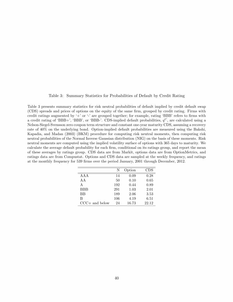
Table 3: Summary Statistics for Probabilities of Default by Credit Rating

Table 3 presents summary statistics for risk neutral probabilities of default implied by credit default swap(CDS) spreads and prices of options on the equity of the same firm, grouped by credit rating. Firms withcredit ratings augmented by ‘+’ or ‘-’ are grouped together; for example, rating ‘BBB’ refers to firms witha credit rating of ‘BBB+’, ‘BBB’, or ‘BBB-’. CDS-implied default probabilities, qC , are calculated using aNelson-Siegel-Svensson zero coupon term structure and constant one-year maturity CDS, assuming a recoveryrate of 40% on the underlying bond. Option-implied default probabilities are measured using the Bakshi,Kapadia, and Madan (2003) (BKM) procedure for computing risk neutral moments, then computing riskneutral probabilities of the Normal Inverse Gaussian distribution (NIG) on the basis of these moments. Riskneutral moments are computed using the implied volatility surface of options with 365 days to maturity. Wecalculate the average default probability for each firm, conditional on its ratings group, and report the meanof these averages by ratings group. CDS data are from Markit, options data are from OptionMetrics, andratings data are from Compustat. Options and CDS data are sampled at the weekly frequency, and ratingsat the monthly frequency for 539 firms over the period January, 2001 through December, 2012.

N Option CDS

AAA 14 0.09 0.28AA 50 0.10 0.65A 192 0.44 0.89BBB 291 1.03 2.01BB 189 2.06 3.53B 106 4.19 6.51CCC+ and below 24 16.73 22.12

40

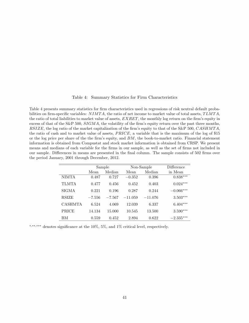
Table 4: Summary Statistics for Firm Characteristics

Table 4 presents summary statistics for firm characteristics used in regressions of risk neutral default proba-bilities on firm-specific variables: NIMTA, the ratio of net income to market value of total assets, TLMTA,the ratio of total liabilities to market value of assets, EXRET , the monthly log return on the firm’s equity inexcess of that of the S&P 500, SIGMA, the volatility of the firm’s equity return over the past three months,RSIZE, the log ratio of the market capitalization of the firm’s equity to that of the S&P 500, CASHMTA,the ratio of cash and to market value of assets, PRICE, a variable that is the maximum of the log of $15or the log price per share of the the firm’s equity, and BM , the book-to-market ratio. Financial statementinformation is obtained from Compustat and stock market information is obtained from CRSP. We presentmeans and medians of each variable for the firms in our sample, as well as the set of firms not included inour sample. Differences in means are presented in the final column. The sample consists of 502 firms overthe period January, 2001 through December, 2012.

Sample Non-Sample DifferenceMean Median Mean Median in Mean

NIMTA 0.487 0.727 −0.352 0.396 0.838∗∗∗

TLMTA 0.477 0.456 0.452 0.403 0.024∗∗∗

SIGMA 0.221 0.196 0.287 0.244 −0.066∗∗∗

RSIZE −7.556 −7.567 −11.059 −11.076 3.503∗∗∗

CASHMTA 6.524 4.069 12.039 6.337 6.404∗∗∗

PRICE 14.134 15.000 10.545 13.500 3.590∗∗∗

BM 0.559 0.452 2.894 0.622 −2.335∗∗∗

∗,∗∗,∗∗∗ denotes significance at the 10%, 5%, and 1% critical level, respectively.

41

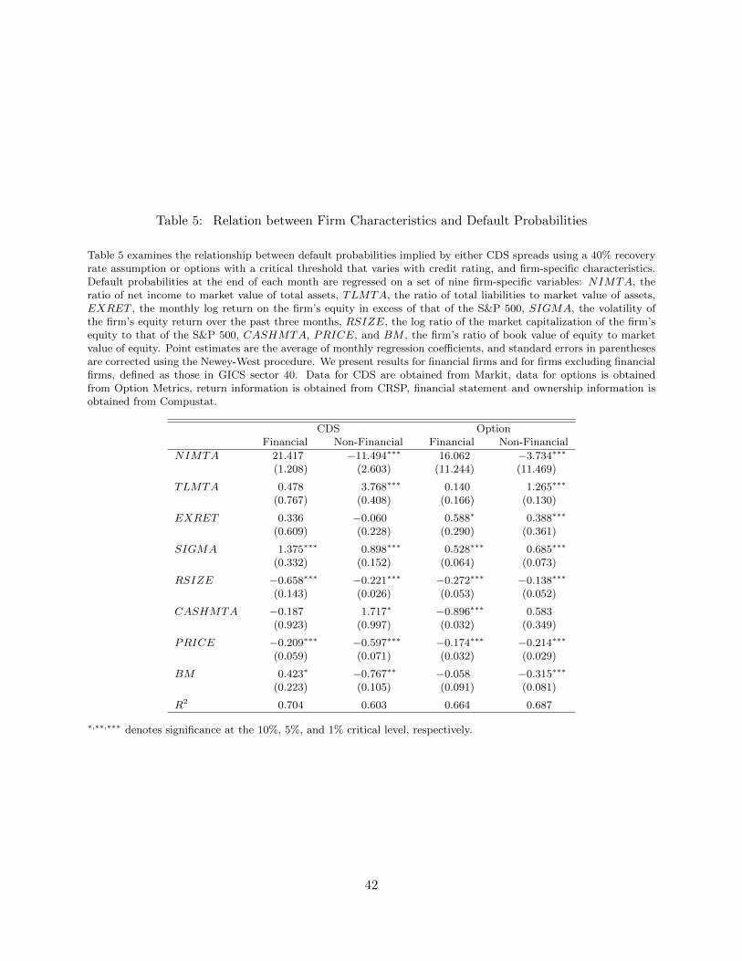
Table 5: Relation between Firm Characteristics and Default Probabilities

Table 5 examines the relationship between default probabilities implied by either CDS spreads using a 40% recoveryrate assumption or options with a critical threshold that varies with credit rating, and firm-specific characteristics.Default probabilities at the end of each month are regressed on a set of nine firm-specific variables: NIMTA, theratio of net income to market value of total assets, TLMTA, the ratio of total liabilities to market value of assets,EXRET , the monthly log return on the firm’s equity in excess of that of the S&P 500, SIGMA, the volatility ofthe firm’s equity return over the past three months, RSIZE, the log ratio of the market capitalization of the firm’sequity to that of the S&P 500, CASHMTA, PRICE, and BM , the firm’s ratio of book value of equity to marketvalue of equity. Point estimates are the average of monthly regression coefficients, and standard errors in parenthesesare corrected using the Newey-West procedure. We present results for financial firms and for firms excluding financialfirms, defined as those in GICS sector 40. Data for CDS are obtained from Markit, data for options is obtainedfrom Option Metrics, return information is obtained from CRSP, financial statement and ownership information isobtained from Compustat.

CDS OptionFinancial Non-Financial Financial Non-Financial

NIMTA 21.417 −11.494∗∗∗ 16.062 −3.734∗∗∗

(1.208) (2.603) (11.244) (11.469)

TLMTA 0.478 3.768∗∗∗ 0.140 1.265∗∗∗

(0.767) (0.408) (0.166) (0.130)

EXRET 0.336 −0.060 0.588∗ 0.388∗∗∗

(0.609) (0.228) (0.290) (0.361)

SIGMA 1.375∗∗∗ 0.898∗∗∗ 0.528∗∗∗ 0.685∗∗∗

(0.332) (0.152) (0.064) (0.073)

RSIZE −0.658∗∗∗ −0.221∗∗∗ −0.272∗∗∗ −0.138∗∗∗

(0.143) (0.026) (0.053) (0.052)

CASHMTA −0.187 1.717∗ −0.896∗∗∗ 0.583(0.923) (0.997) (0.032) (0.349)

PRICE −0.209∗∗∗ −0.597∗∗∗ −0.174∗∗∗ −0.214∗∗∗

(0.059) (0.071) (0.032) (0.029)

BM 0.423∗ −0.767∗∗ −0.058 −0.315∗∗∗

(0.223) (0.105) (0.091) (0.081)

R2 0.704 0.603 0.664 0.687

∗,∗∗,∗∗∗ denotes significance at the 10%, 5%, and 1% critical level, respectively.

42

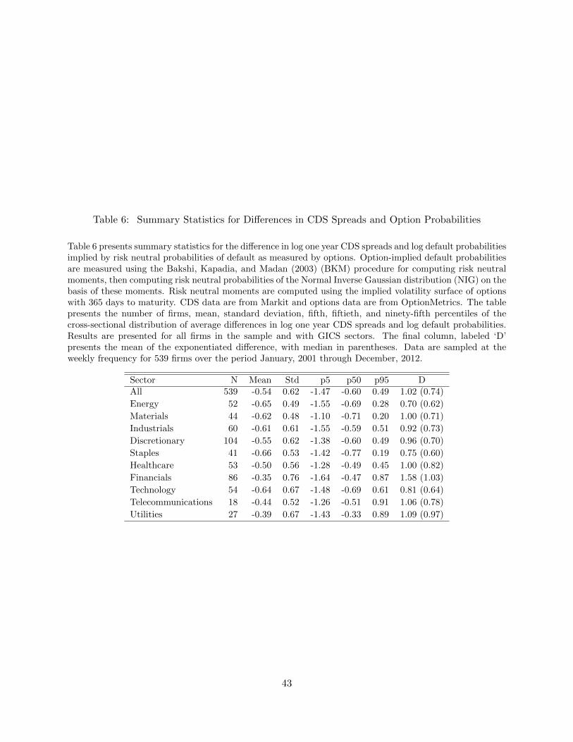
Table 6: Summary Statistics for Differences in CDS Spreads and Option Probabilities

Table 6 presents summary statistics for the difference in log one year CDS spreads and log default probabilitiesimplied by risk neutral probabilities of default as measured by options. Option-implied default probabilitiesare measured using the Bakshi, Kapadia, and Madan (2003) (BKM) procedure for computing risk neutralmoments, then computing risk neutral probabilities of the Normal Inverse Gaussian distribution (NIG) on thebasis of these moments. Risk neutral moments are computed using the implied volatility surface of optionswith 365 days to maturity. CDS data are from Markit and options data are from OptionMetrics. The tablepresents the number of firms, mean, standard deviation, fifth, fiftieth, and ninety-fifth percentiles of thecross-sectional distribution of average differences in log one year CDS spreads and log default probabilities.Results are presented for all firms in the sample and with GICS sectors. The final column, labeled ‘D’presents the mean of the exponentiated difference, with median in parentheses. Data are sampled at theweekly frequency for 539 firms over the period January, 2001 through December, 2012.

Sector N Mean Std p5 p50 p95 DAll 539 -0.54 0.62 -1.47 -0.60 0.49 1.02 (0.74)

Energy 52 -0.65 0.49 -1.55 -0.69 0.28 0.70 (0.62)

Materials 44 -0.62 0.48 -1.10 -0.71 0.20 1.00 (0.71)

Industrials 60 -0.61 0.61 -1.55 -0.59 0.51 0.92 (0.73)

Discretionary 104 -0.55 0.62 -1.38 -0.60 0.49 0.96 (0.70)

Staples 41 -0.66 0.53 -1.42 -0.77 0.19 0.75 (0.60)

Healthcare 53 -0.50 0.56 -1.28 -0.49 0.45 1.00 (0.82)

Financials 86 -0.35 0.76 -1.64 -0.47 0.87 1.58 (1.03)

Technology 54 -0.64 0.67 -1.48 -0.69 0.61 0.81 (0.64)

Telecommunications 18 -0.44 0.52 -1.26 -0.51 0.91 1.06 (0.78)

Utilities 27 -0.39 0.67 -1.43 -0.33 0.89 1.09 (0.97)

43

Table 7: Differences in CDS Spreads and Option-Implied Probabilities and Firm Characteristics

Table 7 examines the relationship between the difference in log one-year CDS spreads and log option-implieddefault probabilities and firm-specific characteristics. Differences are regressed on a set of nine firm-specificvariables: NIMTA, the ratio of net income to market value of total assets, TLMTA, the ratio of totalliabilities to market value of assets, EXRET , the monthly log return on the firm’s equity in excess of thatof the S&P 500, SIGMA, the volatility of the firm’s equity return over the past three months, RSIZE, thelog ratio of the market capitalization of the firm’s equity to that of the S&P 500, CASHMTA, PRICE, avariable that is the maximum of the log of $15 or the log price per share of the the firm’s equity, INST ,the fraction of shares owned by insititutions, and NSHARE, the number of shareholders divided by marketvalue of equity. Additionally, one of four measures of liquidation costs are included: NONFIXED, oneminus the ratio of net property, plant, and equipment to total assets, BM , the firm’s ratio of book value ofequity to market value of equity, TANG, the measure of asset tangibility from Almeida and Campello (2007),and R&D, the ratio of research and development expenses to investment. Standard errors are presentedin parentheses below point estimates. Data for CDS are obtained from Markit, data on options fromOptionMetrics, return information is obtained from CRSP, financial statement and ownership informationis obtained from COMPUSTAT.

(1) (2) (3) (1)NIMTA −4.625∗∗∗ −3.869∗∗∗ −3.937∗∗∗ −4.142∗∗∗

(0.963) (0.787) (0.845) (0.851)

TLMTA 1.128∗∗∗ 1.023∗∗∗ 1.062∗∗∗ 1.023∗∗∗

(0.084) (0.089) (0.081) (0.077)

EXRET 0.009 0.011 0.004 −0.023(0.081) (0.081) (0.085) (0.082)

SIGMA 0.260∗∗∗ 0.272∗∗∗ 0.279∗∗∗ 0.271∗∗∗

(0.036) (0.034) (0.035) (0.034)

RSIZE −0.309∗∗∗ −0.317∗∗∗ −0.320∗∗∗ −0.321∗∗∗

(0.021) (0.020) (0.021) (0.022)

CASHMTA −0.743∗∗ −1.151∗∗∗ −0.909∗∗∗ −1.142∗∗∗

(0.360) (0.353) (0.346) (0.386)

PRICE −0.206∗ −0.137∗∗ −0.178∗ −0.186∗

(0.124) (0.055) (0.095) (0.100)

NONFIXED −0.368∗∗∗

(0.053)

BM 0.080∗

(0.047)

TANG −0.347∗∗∗

(0.099)

R&D −0.033∗∗∗

(0.009)

INST 0.024 −0.043 −0.027 −0.041(0.133) (0.138) (0.137) (0.146)

NSHARE −3.632∗∗∗ −3.485∗∗∗ −3.684∗∗∗ −3.893∗∗∗

(0.857) (0.928) (0.897) (0.854)

R2 0.589 0.582 0.584 0.582

44

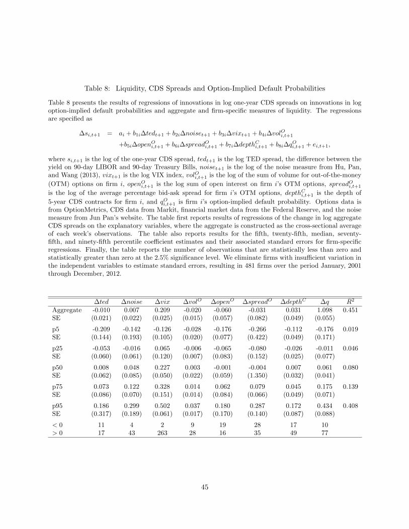
Table 8: Liquidity, CDS Spreads and Option-Implied Default Probabilities

Table 8 presents the results of regressions of innovations in log one-year CDS spreads on innovations in logoption-implied default probabilities and aggregate and firm-specific measures of liquidity. The regressionsare specified as

∆si,t+1 = ai + b1i∆tedt+1 + b2i∆noiset+1 + b3i∆vixt+1 + b4i∆volOi,t+1

+b5i∆openOi,t+1 + b6i∆spread

Oi,t+1 + b7i∆depth

Ci,t+1 + b8i∆q

Oi,t+1 + ei,t+1,

where si,t+1 is the log of the one-year CDS spread, tedt+1 is the log TED spread, the difference between theyield on 90-day LIBOR and 90-day Treasury Bills, noiset+1 is the log of the noise measure from Hu, Pan,and Wang (2013), vixt+1 is the log VIX index, volOi,t+1 is the log of the sum of volume for out-of-the-money

(OTM) options on firm i, openOi,t+1 is the log sum of open interest on firm i’s OTM options, spreadOi,t+1

is the log of the average percentage bid-ask spread for firm i’s OTM options, depthCi,t+1 is the depth of

5-year CDS contracts for firm i, and qOi,t+1 is firm i’s option-implied default probability. Options data isfrom OptionMetrics, CDS data from Markit, financial market data from the Federal Reserve, and the noisemeasure from Jun Pan’s website. The table first reports results of regressions of the change in log aggregateCDS spreads on the explanatory variables, where the aggregate is constructed as the cross-sectional averageof each week’s observations. The table also reports results for the fifth, twenty-fifth, median, seventy-fifth, and ninety-fifth percentile coefficient estimates and their associated standard errors for firm-specificregressions. Finally, the table reports the number of observations that are statistically less than zero andstatistically greater than zero at the 2.5% significance level. We eliminate firms with insufficient variation inthe independent variables to estimate standard errors, resulting in 481 firms over the period January, 2001through December, 2012.

∆ted ∆noise ∆vix ∆volO ∆openO ∆spreadO ∆depthC ∆q R2

Aggregate -0.010 0.007 0.209 -0.020 -0.060 -0.031 0.031 1.098 0.451SE (0.021) (0.022) (0.025) (0.015) (0.057) (0.082) (0.049) (0.055)

p5 -0.209 -0.142 -0.126 -0.028 -0.176 -0.266 -0.112 -0.176 0.019SE (0.144) (0.193) (0.105) (0.020) (0.077) (0.422) (0.049) (0.171)

p25 -0.053 -0.016 0.065 -0.006 -0.065 -0.080 -0.026 -0.011 0.046SE (0.060) (0.061) (0.120) (0.007) (0.083) (0.152) (0.025) (0.077)

p50 0.008 0.048 0.227 0.003 -0.001 -0.004 0.007 0.061 0.080SE (0.062) (0.085) (0.050) (0.022) (0.059) (1.350) (0.032) (0.041)

p75 0.073 0.122 0.328 0.014 0.062 0.079 0.045 0.175 0.139SE (0.086) (0.070) (0.151) (0.014) (0.084) (0.066) (0.049) (0.071)

p95 0.186 0.299 0.502 0.037 0.180 0.287 0.172 0.434 0.408SE (0.317) (0.189) (0.061) (0.017) (0.170) (0.140) (0.087) (0.088)

< 0 11 4 2 9 19 28 17 10> 0 17 43 263 28 16 35 49 77

45

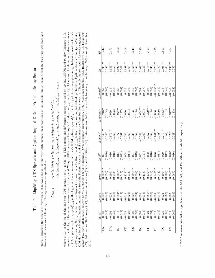
Tab

le9:

Liq

uid

ity,

CD

SS

pre

ads

and

Opti

on-I

mp

lied

Def

ault

Pro

bab

ilit

ies

by

Sec

tor

Tab

le9

pre

sents

the

resu

lts

of

regre

ssio

ns

of

inn

ovati

on

sin

log

on

e-yea

rC

DS

spre

ad

son

inn

ovati

on

sin

log

op

tion

-im

plied

def

au

ltp

rob

ab

ilit

ies

an

daggre

gate

an

dfi

rm-s

pec

ific

mea

sure

sof

liqu

idit

y.T

he

regre

ssio

ns

are

spec

ified

as

∆s i

,t+1

=ai

+b 1

i∆tedt+

1+b 2

i∆noise t

+1

+b 3

i∆vix

t+1

+b 4

i∆volO i,

t+1

+b 5

i∆open

O i,t+

1+b 6

i∆spreadO i,t+

1+b 7

i∆depth

C i,t+

1+b 8

i∆qO i,t+

1+e i

,t+1,

wh

eres i

,t+1

isth

elo

gof

the

on

e-yea

rC

DS

spre

ad

,tedt+

1is

the

log

TE

Dsp

read

,th

ed

iffer

ence

bet

wee

nth

eyie

ldon

90-d

ay

LIB

OR

an

d90-d

ay

Tre

asu

ryB

ills

,noise t

+1

isth

elo

gof

the

nois

em

easu

refr

om

Hu

,P

an

,an

dW

an

g(2

013),vix

t+1

isth

elo

gV

IXin

dex

,volO i,

t+1

isth

elo

gof

the

sum

of

volu

me

for

ou

t-of-

the-

mon

ey

(OT

M)

op

tion

son

firm

i,open

O i,t+

1is

the

log

sum

of

op

enin

tere

ston

firm

i’s

OT

Mop

tion

s,spreadO i,t+

1is

the

log

of

the

aver

age

per

centa

ge

bid

-ask

spre

ad

for

firm

i’s

OT

Mop

tion

s,depth

C i,t+

1is

the

dep

thof

5-y

ear

CD

Sco

ntr

act

sfo

rfi

rmi,

an

dqO i,t+

1is

firm

i’s

op

tion

-im

plied

def

au

ltp

rob

ab

ilit

y.O

pti

on

sd

ata

isfr

om

Op

tion

Met

rics

,C

DS

data

from

Mark

it,

fin

an

cial

mark

etd

ata

from

the

Fed

eral

Res

erve,

an

dth

en

ois

em

easu

refr

om

Ju

nP

an

’sw

ebsi

te.

Th

eta

ble

rep

ort

sre

sult

sfo

rse

ries

aggre

gate

dacr

oss

two-d

igit

GIC

Sco

des

,E

ner

gy

(EN

),M

ate

rials

(MA

),In

du

stri

als

(IN

),C

on

sum

erD

iscr

etio

nary

(CD

),C

on

sum

erS

tap

les

(CS

),H

ealt

hca

re(HC

),F

inan

cials

(FI),

Info

rmati

on

Tec

hn

olo

gy

(IT

),T

elec

om

mu

nic

ati

on

s(TC

),an

dU

tiliti

es(UT

).D

ata

are

sam

ple

dat

the

wee

kly

freq

uen

cyfr

om

Janu

ary

,2001

thro

ugh

Dec

emb

er,

2012.

∆ted

∆noise

∆vix

∆volO

∆open

O∆spreadO

∆depth

C∆q

R2

EN

0.0

09

0.0

28

0.1

75∗∗∗

0.0

21

0.3

40∗∗∗

0.2

18∗∗

0.0

65

0.9

93∗∗∗

0.4

44

(0.0

42)

(0.0

47)

(0.0

50)

(0.0

20)

(0.0

49)

(0.1

04)

(0.0

66)

(0.0

53)

MA

−0.0

01

0.0

23

0.1

99∗∗∗

0.0

10

−0.1

76∗∗∗

0.0

79

−0.1

11∗∗

1.1

43∗∗∗

0.4

71

(0.0

35)

(0.0

38)

(0.0

43)

(0.0

15)

(0.0

60)

(0.0

93)

(0.0

48)

(0.0

53)

IN−

0.0

13

0.0

94∗∗

0.1

26∗∗

−0.0

14

0.0

77

0.2

77∗∗

0.0

68

1.1

22∗∗∗

0.5

62

(0.0

41)

(0.0

44)

(0.0

49)

(0.0

21)

(0.0

81)

(0.1

27)

(0.0

68)

(0.0

42)

CD

−0.0

34

−0.0

15

0.2

23∗∗∗

0.0

08

−0.0

89

0.0

50

0.0

35

1.1

91∗∗∗

0.4

18

(0.0

27)

(0.0

29)

(0.0

33)

(0.0

14)

(0.0

60)

(0.0

91)

(0.0

50)

(0.0

63)

CS

−0.0

02

0.0

28

0.1

90∗∗∗

0.0

21

0.0

35

−0.1

03

0.0

45

0.9

64∗∗∗

0.3

45

(0.0

32)

(0.0

34)

(0.0

38)

(0.0

13)

(0.0

54)

(0.1

05)

(0.0

55)

(0.0

59)

HC

0.0

04

0.0

01

0.0

71∗

0.0

01

−0.0

48

0.6

04∗∗∗

0.0

68

0.4

08∗∗∗

0.2

80

(0.0

35)

(0.0

38)

(0.4

18)

(0.1

77)

(0.0

60)

(0.0

97)

(0.0

57)

(0.0

33)

FI

−0.0

24

0.0

86∗∗

0.2

79∗∗∗

−0.0

02

−0.0

67

0.3

20∗∗∗

−0.0

08

0.7

16∗∗∗

0.4

55

(0.0

34)

(0.0

36)

(0.0

41)

(0.0

16)

(0.0

59)

(0.1

05)

(0.0

51)

(0.0

36)

IT0.0

15

−0.0

09

0.1

43∗∗∗

0.0

26

−0.1

41∗∗∗

−0.0

06

−0.1

28∗∗∗

0.9

70∗∗∗

0.4

25

(0.0

35)

(0.0

37)

(0.0

42)

(0.0

17)

(0.0

48)

(0.0

99)

(0.0

51)

(0.0

50)

TC

0.0

29

−0.0

22

0.2

01∗∗∗

0.0

20

−0.2

70∗∗∗

0.5

52∗∗∗

−0.0

38

0.9

05∗∗∗

0.5

11

(0.0

58)

(0.0

62)

(0.0

69)

(0.0

17)

(0.0

54)

(0.1

01)

(0.0

45)

(0.0

40)

UT

0.0

11

0.0

67

0.2

36∗∗∗

0.0

28∗

0.0

74∗

0.3

77∗∗∗

−0.0

40

0.7

96∗∗∗

0.4

84

(0.0

60)

(0.0

61)

(0.0

67)

(0.0

16)

(0.0

41)

(0.1

15)

(0.0

58)

(0.0

52)

∗,∗∗

,∗∗∗

rep

rese

nt

stati

stic

al

sign

ifica

nce

at

the

10%

,5%

,an

d1%

crit

ical

thre

shold

,re

spec

tivel

y.

46

Tab

le10

:P

red

icta

bil

ity

ofR

etu

rns

by

CD

S-

and

Op

tion

-Im

pli

edP

rob

abil

itie

san

dth

eir

Diff

eren

ce

The

table

pre

sents

the

resu

lts

of

regre

ssio

ns,

r p,t+1

=a

+b∆

xp,t

+e p

,t,

wher

er p

,t+1

isth

elo

gre

turn

on

an

index

,xp,t

={q

C p,t,q

O p,t,q

C p,t−

qO p,t}

is,

dep

endin

gon

spec

ifica

tion,

the

log

CD

S-i

mplied

risk

neu

tral

pro

babilit

yof

def

ault

,th

elo

gopti

on-i

mplied

risk

neu

tral

pro

babilit

yof

def

ault

,or

the

diff

eren

cein

the

log

pro

babilit

ies

of

def

ault

.P

redic

tive

regre

ssio

ns

are

per

form

edfo

rth

eC

RSP

valu

e-w

eighte

din

dex

and

indic

esof

10

sect

ors

;E

ner

gy

(EN

),M

ate

rials

(MA

),In

dust

rials

(IN

),C

onsu

mer

Dis

cret

ionary

(CD

),C

onsu

mer

Sta

ple

s(C

S),

Hea

lthca

re(H

C),

Fin

anci

als

(FI)

,In

form

ati

on

Tec

hnolo

gy

(IT

),T

elec

om

munic

ati

ons

(TC

),and

Uti

liti

es(U

T).

The

table

pre

sents

slop

eco

effici

ents

,ass

oci

ate

dst

andard

erro

rs,

andR

2fo

runiv

ari

ate

regre

ssio

ns

of

retu

rns

on

the

vari

able

s.D

ata

are

sam

ple

dat

the

wee

kly

freq

uen

cyfr

om

January

,2001

thro

ugh

Dec

emb

er,

2012.

qCSE

R2

qOSE

R2

qC−

qOSE

R2

Aggre

gate

1.8

26

(1.2

20)

0.3

58

0.1

70

(3.2

73)

0.0

00

3.6

90∗∗

(1.7

76)

0.6

89

EN

0.1

51

(0.9

79)

0.0

04

−2.4

36

(1.5

33)

0.4

11

3.4

65∗∗

(1.6

04)

0.7

58

MA

2.2

91∗∗

(0.9

97)

0.8

41

1.3

77

(1.7

34)

0.1

01

3.3

86∗∗

(1.4

38)

0.8

83

IN0.7

17

(0.7

50)

0.1

47

0.1

81

(0.9

86)

0.0

05

3.7

62∗∗

(1.4

74)

1.0

36

CD

2.7

33∗

(1.4

81)

0.5

45

1.9

44

(2.5

68)

0.0

92

2.1

11

(2.0

68)

0.1

67

CS

0.4

24

(0.6

20)

0.0

75

−0.9

12

(1.0

57)

0.1

19

1.6

66∗

(0.8

92)

0.5

59

HC

−0.8

63

(0.8

16)

0.1

81

−0.7

78

(0.7

17)

0.1

90

−0.0

49

(0.9

11)

0.0

00

FI

3.4

97∗∗∗

(1.1

97)

1.3

53

0.3

84

(1.3

50)

0.0

13

5.4

91∗∗∗

(1.8

39)

1.4

13

IT−

0.9

28

(1.0

24)

0.1

32

0.5

33

(1.5

74)

0.0

18

−2.8

18∗∗

(1.4

23)

0.6

26

TC

−0.5

45

(0.4

62)

0.2

23

−0.5

39

(0.6

35)

0.1

16

−0.3

11

(0.7

33)

0.0

29

UT

−1.7

45∗

(1.0

05)

0.4

93

−2.8

07∗∗

(1.3

85)

0.6

70

−1.2

04

(1.5

49)

0.0

99

47

Figure 1: Implied Default Probabilities

Figure 1 plots the time series of aggregate default probabilities. Default probabilities are measured using

one year CDS spreads with an assumed recovery rate of 40% and using the risk neutral distribution implied

by option prices with a ratings-dependent critical threshold and a constant threshold α = 0.05. CDS data

are obtained from Markit and options data from OptionMetrics. Data are sampled at the weekly frequency

and aggregated by taking the average across the firms in the sample. The data cover the period January,

2001 through December, 2012, and cover 539 firms.

2001 2002 2003 2004 2005 2006 2007 2008 2009 2010 2011 2012 2013 2014

Date

0

0.01

0.02

0.03

0.04

0.05

0.06

Ris

k N

eu

tra

l D

efa

ult P

rob

ab

ility

CDS

Flexible Threshold

=0.15

48

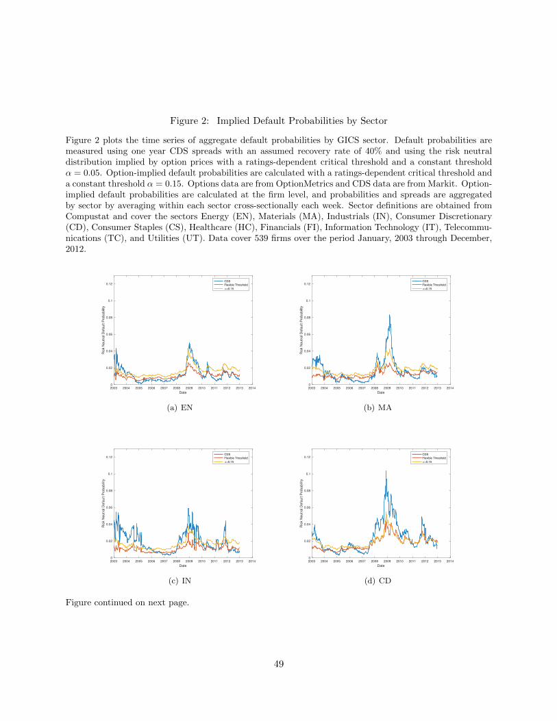
Figure 2: Implied Default Probabilities by Sector

Figure 2 plots the time series of aggregate default probabilities by GICS sector. Default probabilities aremeasured using one year CDS spreads with an assumed recovery rate of 40% and using the risk neutraldistribution implied by option prices with a ratings-dependent critical threshold and a constant thresholdα = 0.05. Option-implied default probabilities are calculated with a ratings-dependent critical threshold anda constant threshold α = 0.15. Options data are from OptionMetrics and CDS data are from Markit. Option-implied default probabilities are calculated at the firm level, and probabilities and spreads are aggregatedby sector by averaging within each sector cross-sectionally each week. Sector definitions are obtained fromCompustat and cover the sectors Energy (EN), Materials (MA), Industrials (IN), Consumer Discretionary(CD), Consumer Staples (CS), Healthcare (HC), Financials (FI), Information Technology (IT), Telecommu-nications (TC), and Utilities (UT). Data cover 539 firms over the period January, 2003 through December,2012.

2003 2004 2005 2006 2007 2008 2009 2010 2011 2012 2013 2014

Date

0

0.02

0.04

0.06

0.08

0.1

0.12

Ris

k N

eutr

al D

efa

ult P

robabili

ty

CDS

Flexible Threshold

=0.15

(a) EN

2003 2004 2005 2006 2007 2008 2009 2010 2011 2012 2013 2014

Date

0

0.02

0.04

0.06

0.08

0.1

0.12

Ris

k N

eutr

al D

efa

ult P

robabili

ty

CDS

Flexible Threshold

=0.15

(b) MA

2003 2004 2005 2006 2007 2008 2009 2010 2011 2012 2013 2014

Date

0

0.02

0.04

0.06

0.08

0.1

0.12

Ris

k N

eutr

al D

efa

ult P

robabili

ty

CDS

Flexible Threshold

=0.15

(c) IN

2003 2004 2005 2006 2007 2008 2009 2010 2011 2012 2013 2014

Date

0

0.02

0.04

0.06

0.08

0.1

0.12

Ris

k N

eutr

al D

efa

ult P

robabili

ty

CDS

Flexible Threshold

=0.15

(d) CD

Figure continued on next page.

49

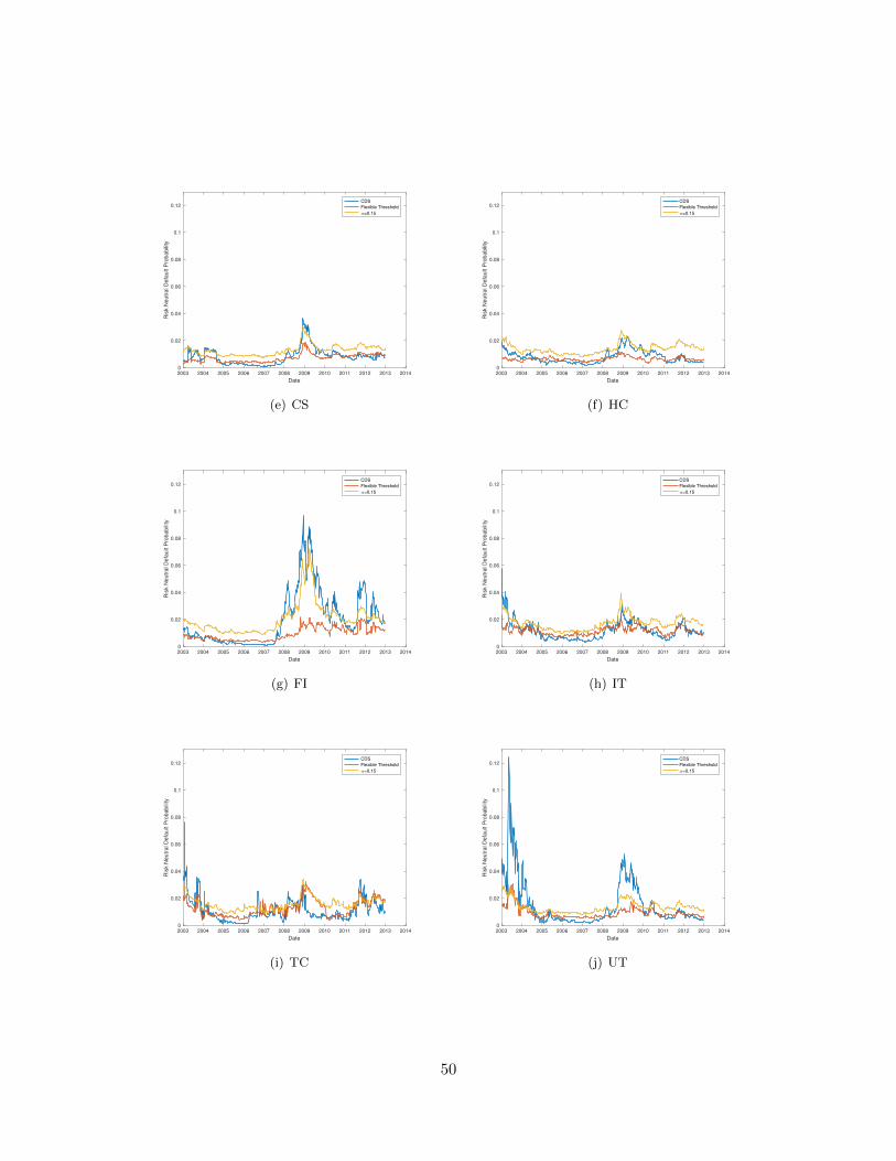
2003 2004 2005 2006 2007 2008 2009 2010 2011 2012 2013 2014

Date

0

0.02

0.04

0.06

0.08

0.1

0.12

Ris

k N

eutr

al D

efa

ult P

robabili

ty

CDS

Flexible Threshold

=0.15

(e) CS

2003 2004 2005 2006 2007 2008 2009 2010 2011 2012 2013 2014

Date

0

0.02

0.04

0.06

0.08

0.1

0.12

Ris

k N

eutr

al D

efa

ult P

robabili

ty

CDS

Flexible Threshold

=0.15

(f) HC

2003 2004 2005 2006 2007 2008 2009 2010 2011 2012 2013 2014

Date

0

0.02

0.04

0.06

0.08

0.1

0.12

Ris

k N

eutr

al D

efa

ult P

robabili

ty

CDS

Flexible Threshold

=0.15

(g) FI

2003 2004 2005 2006 2007 2008 2009 2010 2011 2012 2013 2014

Date

0

0.02

0.04

0.06

0.08

0.1

0.12R

isk N

eutr

al D

efa

ult P

robabili

tyCDS

Flexible Threshold

=0.15

(h) IT

2003 2004 2005 2006 2007 2008 2009 2010 2011 2012 2013 2014

Date

0

0.02

0.04

0.06

0.08

0.1

0.12

Ris

k N

eutr

al D

efa

ult P

robabili

ty

CDS

Flexible Threshold

=0.15

(i) TC

2003 2004 2005 2006 2007 2008 2009 2010 2011 2012 2013 2014

Date

0

0.02

0.04

0.06

0.08

0.1

0.12

Ris

k N

eutr

al D

efa

ult P

robabili

ty

CDS

Flexible Threshold

=0.15

(j) UT

50

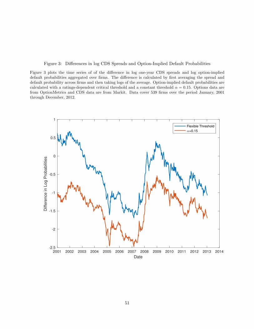
Figure 3: Differences in log CDS Spreads and Option-Implied Default Probabilities

Figure 3 plots the time series of of the difference in log one-year CDS spreads and log option-implieddefault probabilities aggregated over firms. The difference is calculated by first averaging the spread anddefault probability across firms and then taking logs of the average. Option-implied default probabilities arecalculated with a ratings-dependent critical threshold and a constant threshold α = 0.15. Options data arefrom OptionMetrics and CDS data are from Markit. Data cover 539 firms over the period January, 2001through December, 2012.

2001 2002 2003 2004 2005 2006 2007 2008 2009 2010 2011 2012 2013 2014

Date

-2.5

-2

-1.5

-1

-0.5

0

0.5

1

Diffe

ren

ce

in

Lo

g P

rob

ab

ilitie

s

Flexible Threshold

=0.15

51

Figure 4: Differences in log CDS Spreads and Option-Implied Default Probabilities by Sector

Figure 4 presents the difference in the log of one-year CDS spreads and the log of option-implied defaultprobabilities aggregated by GICS sector. Option-implied default probabilities are calculated with a ratings-dependent critical threshold and a constant threshold α = 0.15. Options data are from OptionMetricsand CDS data are from Markit. Option-implied default probabilities are calculated at the firm level, andprobabilities and spreads are aggregated by sector by averaging within each sector cross-sectionally eachweek. Sector definitions are obtained from Compustat and cover the sectors Energy (EN), Materials (MA),Industrials (IN), Consumer Discretionary (CD), Consumer Staples (CS), Healthcare (HC), Financials (FI),Information Technology (IT), Telecommunications (TC), and Utilities (UT). Data cover 539 firms over theperiod January, 2003 through December, 2012.

2003 2004 2005 2006 2007 2008 2009 2010 2011 2012 2013 2014

Date

-3

-2.5

-2

-1.5

-1

-0.5

0

0.5

1

1.5

Diffe

rence in L

og P

robabili

ties

Flexible Threshold

=0.15

(a) EN

2003 2004 2005 2006 2007 2008 2009 2010 2011 2012 2013 2014

Date

-3

-2.5

-2

-1.5

-1

-0.5

0

0.5

1

1.5

Diffe

rence in L

og P

robabili

ties

Flexible Threshold

=0.15

(b) MA

2003 2004 2005 2006 2007 2008 2009 2010 2011 2012 2013 2014

Date

-3

-2.5

-2

-1.5

-1

-0.5

0

0.5

1

1.5

Diffe

rence in L

og P

robabili

ties

Flexible Threshold

=0.15

(c) IN

2003 2004 2005 2006 2007 2008 2009 2010 2011 2012 2013 2014

Date

-3

-2.5

-2

-1.5

-1

-0.5

0

0.5

1

1.5

Diffe

rence in L

og P

robabili

ties

Flexible Threshold

=0.15

(d) CD

Figure continued on next page.

52

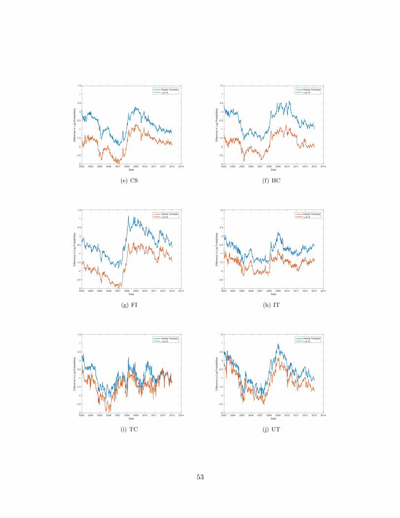
2003 2004 2005 2006 2007 2008 2009 2010 2011 2012 2013 2014

Date

-3

-2.5

-2

-1.5

-1

-0.5

0

0.5

1

1.5

Diffe

rence in L

og P

robabili

ties

Flexible Threshold

=0.15

(e) CS

2003 2004 2005 2006 2007 2008 2009 2010 2011 2012 2013 2014

Date

-3

-2.5

-2

-1.5

-1

-0.5

0

0.5

1

1.5

Diffe

rence in L

og P

robabili

ties

Flexible Threshold

=0.15

(f) HC

2003 2004 2005 2006 2007 2008 2009 2010 2011 2012 2013 2014

Date

-3

-2.5

-2

-1.5

-1

-0.5

0

0.5

1

1.5

Diffe

rence in L

og P

robabili

ties

Flexible Threshold

=0.15

(g) FI

2003 2004 2005 2006 2007 2008 2009 2010 2011 2012 2013 2014

Date

-3

-2.5

-2

-1.5

-1

-0.5

0

0.5

1

1.5

Diffe

rence in L

og P

robabili

ties

Flexible Threshold

=0.15

(h) IT

2003 2004 2005 2006 2007 2008 2009 2010 2011 2012 2013 2014

Date

-3

-2.5

-2

-1.5

-1

-0.5

0

0.5

1

1.5

Diffe

rence in L

og P

robabili

ties

Flexible Threshold

=0.15

(i) TC

2003 2004 2005 2006 2007 2008 2009 2010 2011 2012 2013 2014

Date

-3

-2.5

-2

-1.5

-1

-0.5

0

0.5

1

1.5

Diffe

rence in L

og P

robabili

ties

Flexible Threshold

=0.15

(j) UT

53