Cross Sections, Data Projection and Dip -Domain Mappingextras.springer.com/2006/978-3-540-31054-9/Data/006.pdf · 134 Chapter 6 · Cross Sections, Data Projection and Dip-Domain Mapping

Chapter 6

6.1Introduction

A cross section shows the relationships between different horizons and allows theinformation from multiple map horizons to be incorporated into the interpretation.Cross sections may categorized as illustrative or predictive. The purpose of an illustra-tive cross section is to illustrate the cross section view of an already-completed map or3-D interpretation. A slice through a 3-D interpretation is a perfect example. The pur-pose of a predictive cross section is to assemble scattered information and, utilizingappropriate rules, predict the geometry between control points. A predictive crosssection can be used to predict the geometry of a horizon for which little or no infor-mation is available.

Data projection is typically part of the cross-section construction process. Relevantdata commonly lie a significant distance from the line of section. Rather than ignorethis information, it can be projected onto the section plane. The quality of the resultdepends on selecting the correct projection direction. This chapter describes how toselect the projection direction and gives several techniques for making the projectionby hand or analytically. Projection within a dip-domain style structure involves defin-ing the 3-D axial-surface network and so becomes a blend of mapping, data projection,and section construction.

6.2Cross-Section Preliminaries

6.2.1Choosing the Line of Section

Cross sections constructed for the purpose of structural interpretation are usuallyoriented perpendicular to the fold axis, perpendicular to a major fault, or parallel tothese trends. The structural trend to use in controlling the direction of the cross sec-tion is the axis of the largest fold in the map area or the strike of the major fault inthe area. Good reasons may exist for other choices of the basic design parameters.For example, the cross section may be required in a specific location and directionfor the construction of a road cut or a mine layout. If other choices of the parameters,such as the direction of the section line or the amount of vertical exaggeration, arerequired, it is recommended that a section normal to strike be constructed and vali-

Cross Sections, Data Projection and Dip-Domain Mapping

134 Chapter 6 · Cross Sections, Data Projection and Dip-Domain Mapping

dated (Chap. 10 and 11) first. A grid of cross sections is needed for a complete three-dimensional structural interpretation.

The reason that a structure section should be straight and perpendicular to the majorstructural trend is that it gives the most representative view of the geometry. The sim-plest example of this is a cross section through a circular cylinder (Fig. 6.1). If theentire cylinder is visible, then it would readily be described as being a right circularcylinder. The cross section that best illustrates this description is Fig. 6.1a, normal tothe axis of the cylinder, referred to as the normal section. Any other planar cross sec-tion oblique to the axis is an ellipse (Fig. 6.1b). An elliptical cross section is also correctbut does not convey the appropriate impression of the three dimensional shape of thecylinder. A section that is not straight (Fig. 6.1c) also fails to convey accurately thethree-dimensional geometry of the cylinder, although, again, the section is accurate.Section c in Fig. 6.1 could be improved for structural interpretation by removing thesegment parallel to the axis, producing a section like Fig. 7.1a. A section parallel to thefold (or fault) trend (Fig. 6.1d) is also necessary to completely describe the geometry.

Predictive cross sections are constructed using bed-thickness and fold-curvaturerelationships that are appropriate for the structural style. In order to use these geomet-ric relationships, or rules, to construct and validate cross sections, it is necessary tochoose the cross section to which the rules apply. Such a rule, in the case of the circularcylinder in Fig. 6.1, is that the beds are portions of circular arcs having the same centerof curvature. In this simple and easily applicable form, the rule applies only to section a.More complex rules could be developed for the other cross sections, but it is quickerand less confusing to select the plane of the cross section that fits the simplest rule thanto change the rule to fit an arbitrary cross-section orientation.

Fig. 6.1.Cross sections through a circu-lar cylinder. a Normal section.b Oblique section. c Offsetsection. d Axial section

Fig. 6.2.Structure contour map of ananticline showing the sectionlines. A–A': normal (trans-verse) cross section perpen-dicular to the trend of theanticline. B–B': longitudinalcross section. C–C': well-to-well cross section

135

The effect of a curved section (Fig. 6.2) on the implied geometry of an elongatedome is shown in Fig. 6.3. The correct geometry of the structure is shown by the nor-mal section, a straight-line cross section perpendicular to the axial trace of the struc-ture (Fig. 6.3a) and the longitudinal section (Fig. 6.3b) parallel to the crest of the struc-ture. A line of section that is not straight, such as one that runs through an irregulartrend of wells or a seismic line that follows an irregular road, produces a false imageof the structure. The zig-zag section across the map (Fig. 6.3c) incorrectly shows theanticline to have two local culminations instead of just one. This is a serious problemif the cross section is used to locate hydrocarbon traps or to infer the deep structureusing the predictive section drawing techniques described in Sect. 6.4.

The first line of section across a structure chosen for interpretation should avoidlocal structures, like tear faults, oblique to the main structural trend. Oblique struc-tures introduce complexities into the main structure that are more easily interpretedafter the geometry of the rest of the structure has been determined. Returning to thecylinder, now shown offset along a tear fault (Fig. 6.4), cross sections at a and c will

Fig. 6.3. Sections through the map in Fig. 6.2. a Normal section perpendicular to the fold crest.b Longitudinal section parallel to the fold crest. c Zig-zag or well-to-well cross section. d Oblique3-D view of the structure showing the three cross sections

6.2 · Cross-Section Preliminaries


reveal the basic geometry of the cylinder. A cross section at b that crosses the fault willbe very difficult to interpret until after the basic geometry is known from sections aor c. The simplest method for constructing the structure along section b would be toproject the geometry into it from the unfaulted parts of the cylinder.

6.2.2Choosing the Section Dip

Only a cross section perpendicular to the plunge (the normal section) shows the truebed thicknesses. In all other sections the thicknesses are exaggerated. This is impor-tant if the section is going to be used for predictive purposes. The plunge of a cylin-drical fold is the orientation of its axis, which can be found from the bedding atti-tudes using the stereonet or tangent diagram techniques given in Sect. 5.2. A conicalfold does not have an axis and so, in the strict sense, there is no normal section. Theorientation of either the crestal line or the cone axis is an approximate plunge direc-tion for a conical fold. On a structure contour map the trend and plunge of the crestalline is readily identified. The plunge angle is given by the contour spacing in the plungedirection.

Within a domain of cylindrical folding, changing the dip of the section plane isequivalent to changing the vertical or horizontal exaggeration. This relationship is thebasis of the map interpretation technique known as down-plunge viewing. The mappattern in an area of moderate topographic relief represents an oblique, hence exag-gerated, section through a plunging structure. Viewed in the direction of plunge, themap pattern becomes a normal section (Mackin 1950).

The down-plunge view of a fault should give the correct cross-section geometry andthe sense of the stratigraphic separation. The plunge direction of a fault is parallel tothe axis or crest or trough line of ramp-related folds or drag folds. If the fault is listricor antilistric, the plunge direction should be the axis of the curved surface, just as if itwere a folded surface. If the fault is planar and there are no associated folds, the appro-priate plunge direction is parallel to the cutoff line of a displaced marker against thefault (Threet 1973).

If a vertical cross section is constructed normal to the trend of the plunge, the ver-tical exaggeration due to the plunge angle can be removed by rotating the section usingthe method given in Sect. 6.5. The same approach can be used to convert a map viewinto a normal section.

Fig. 6.4.Cross-section lines across acylinder offset along an ob-lique fault

137

6.2.3Vertical and Horizontal Exaggeration

Both vertical and horizontal exaggeration are used to help visualize and interpret thestructure on cross sections. Vertical exaggeration is a change of the vertical scale (usu-ally an expansion) while maintaining a constant horizontal scale and is a commonmode of presentation of geological cross sections. Vertical exaggeration makes the reliefon a subtle structure more visible on the cross section (Fig. 6.5a). Horizontal exag-geration is a change of the horizontal scale while maintaining a constant vertical scale

Fig. 6.5. Cross sections across Tip Top field, Wyoming thrust belt. a 3: 1 vertical exaggeration and a 0.5 : 1horizontal exaggeration, as might be seen on a seismic reflection profile. b Unexaggerated cross sec-tion. (Section modified from Groshong and Epard 1994, after Webel 1987)



and is common, along with vertical exaggeration, in the presentation of seismic lines(Stone 1991). Reducing the horizontal scale (squeezing) makes a wide, low amplitudestructure more visible and makes the break in horizon continuity at faults more obvi-ous. Squeezing exaggerates the structure without producing an unmanageably tall crosssection.

Vertical exaggeration (Ve) is equal to the length of one unit on the vertical scaledivided by the length of one unit on the map, and horizontal exaggeration (He) is thelength of one unit on the horizontal scale divided by the length of one unit on the map(Fig. 6.6):

Ve = vv / v , (6.1)

He = hh / h , (6.2)

where vv = exaggerated vertical dimension, v = vertical dimension at map scale,hh = exaggerated horizontal dimension, and h = horizontal dimension at map scale.As derived at the end of the chapter (Eqs. 6.21 and 6.22), the true dip is related to theexaggerated dip by

tan δv = Ve tan δ , (6.3)

tan δh = tan δ / He , (6.4)

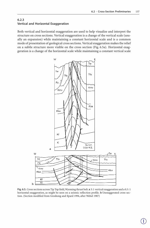
where δv = vertically exaggerated dip, δh = horizontally exaggerated dip, and δ = truedip. Equation 6.3 is plotted in Fig. 6.7. In its effect on the dip, a vertical exaggerationis equivalent to the reciprocal of a horizontal exaggeration (from Eq. 6.24 at the end ofthe chapter):

Ve = 1 / He . (6.5)

Fig. 6.6.Vertical and horizontal exag-geration. A bed of originalthickness t is shown in white.a Unexaggerated cross section.b Horizontally exaggerated(squeezed) cross section.c Vertically exaggerated crosssection

139

The effect of exaggeration on the thickness of a unit is given by (derived as Eqs. 6.26and 6.28)

th / t = cos δh/ cos δ , (6.6)

tv / t = Ve (cos δv / cos δ) . (6.7)

The symbols are the same as in Eqs. 6.1–6.4. Horizontal exaggeration has no effecton the thickness of a horizontal bed, whereas vertical exaggeration changes the thick-ness of a horizontal bed by an amount equal to the exaggeration. Horizontal exaggera-tion changes the thickness of a vertical bed by the full amount of the exaggeration,whereas vertical exaggeration has no effect on the thickness of a vertical bed. For bedsdipping between 0 and 90°, both horizontal and vertical exaggeration cause the appar-ent thickness to increase.

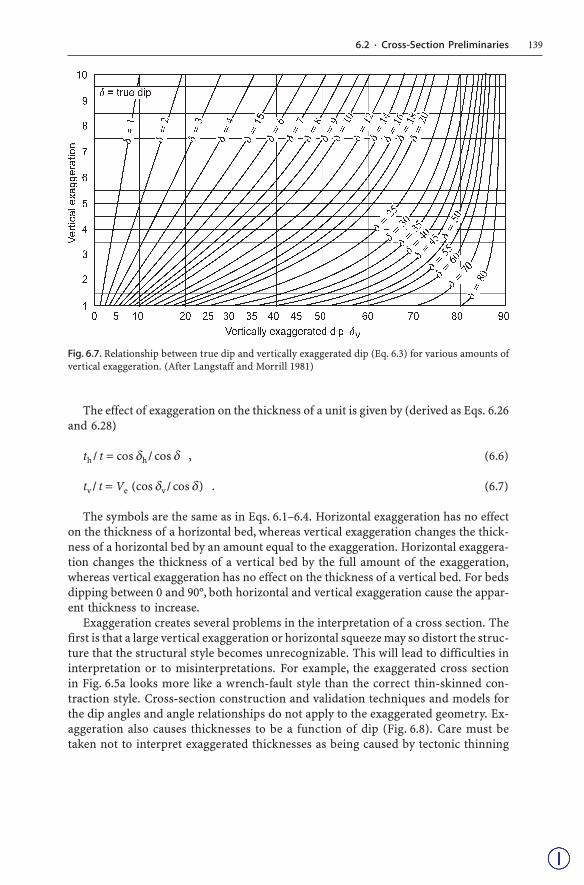
Exaggeration creates several problems in the interpretation of a cross section. Thefirst is that a large vertical exaggeration or horizontal squeeze may so distort the struc-ture that the structural style becomes unrecognizable. This will lead to difficulties ininterpretation or to misinterpretations. For example, the exaggerated cross sectionin Fig. 6.5a looks more like a wrench-fault style than the correct thin-skinned con-traction style. Cross-section construction and validation techniques and models forthe dip angles and angle relationships do not apply to the exaggerated geometry. Ex-aggeration also causes thicknesses to be a function of dip (Fig. 6.8). Care must betaken not to interpret exaggerated thicknesses as being caused by tectonic thinning

Fig. 6.7. Relationship between true dip and vertically exaggerated dip (Eq. 6.3) for various amounts ofvertical exaggeration. (After Langstaff and Morrill 1981)



or thickening or by structural growth during deposition. The profile can be easilycorrected when the true horizontal and vertical scales are known. The correction factoris the inverse of the horizontal or vertical exaggeration. Create an unexaggerated profileby multiplying the correction factor times the scale of the exaggerated axis. If thecross section is in digital form, this is a simple operation using a computer draftingprogram.

Seismic time sections are commonly displayed with both horizontal and verticalexaggerations (Stone 1991). Horizontal exaggeration may be applied to obtain a leg-ible horizontal trace spacing. The amount of horizontal exaggeration is most conve-niently determined by comparing the distance between shot or vibration points markedon the profile with the scale between the corresponding points on the location map.The vertical scale on a time section is in two-way-travel time, and the determinationof the vertical exaggeration requires depth conversion as well as scaling. A few simpletechniques can provide the necessary scaling information without geophysical depthmigration. If the depth to a particular horizon is known independently, as from awell, then the vertical exaggeration at that well can be determined directly from thedefinition (Eq. 6.1). If the true dip is known for a unit or a fault, then the verticalexaggeration can be found by solving Eq. 6.3, given the exaggerated dip from the profile.

If there is a unit on a seismic time section that can be expected to have constantdepositional thickness and minimal structural thickness changes, then any observedthickness change in the unit is caused by the exaggeration (Fig. 6.9a,b). The verticalexaggeration of the time section can be removed by restoring the bed thickness toconstant (Stone 1991). A package of reflectors should be chosen that retains its reflec-tion character and proportional spacing regardless of dip. The reflectors should beparallel to one another and not terminate up or down dip. The thickness changes ofsuch a package are more likely to be caused by exaggeration than by deposition. Asimple procedure for removing the vertical exaggeration is to change the vertical scaleuntil the unit maintains constant thickness regardless of dip (Fig. 6.9c). This pro-vides a quick depth migration that applies to the depth interval over which the unit

Fig. 6.8.Effect of a 3 : 1 vertical exag-geration on thickness. a Pro-file vertically exaggerated 3 : 1.Bed thickness increases as thedip decreases. b Unexagger-ated profile. Bed thickness isconstant

141

occurs. Because seismic velocity varies with depth, the profile might remain exagger-ated at other depths. Normally seismic velocity increases with depth and so the ver-tical exaggeration decreases with depth. This method does not take into accounthorizontal velocity variations. A further caution is that the thickness variations seenin Fig. 6.9a are just like those that are caused by deformation. The inferred verticalexaggeration should always be cross checked by other methods whenever possible. Ifthe profile is also horizontally exaggerated, then this method will give the correctexaggeration ratio of 1 : 1, but both the horizontal and vertical scales could be exag-gerated. Eliminate the horizontal exaggeration while maintaining the ratio constantto produce a depth section.

Fig. 6.9. Time migrated seismic profile from central Wyoming. TWT: Two-way travel time; Ti: intervalthickness. a Original profile having a vertical scale of 7.5 in per second and a horizontal scale of 12 tracesper in. Vertical exaggeration (ve) is 1.87 : 1. b The vertical scale is the same as in a, the horizontal scaleis reduced by two-thirds. Vertical exaggeration is 5.6 : 1. c Unexaggerated version produced by expand-ing the horizontal scale. Thickness T1 is now constant across the profile. (After Stone 1991)



6.3Illustrative Cross Sections

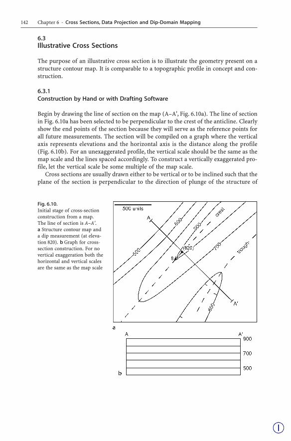
The purpose of an illustrative cross section is to illustrate the geometry present on astructure contour map. It is comparable to a topographic profile in concept and con-struction.

6.3.1Construction by Hand or with Drafting Software

Begin by drawing the line of section on the map (A–A', Fig. 6.10a). The line of sectionin Fig. 6.10a has been selected to be perpendicular to the crest of the anticline. Clearlyshow the end points of the section because they will serve as the reference points forall future measurements. The section will be compiled on a graph where the verticalaxis represents elevations and the horizontal axis is the distance along the profile(Fig. 6.10b). For an unexaggerated profile, the vertical scale should be the same as themap scale and the lines spaced accordingly. To construct a vertically exaggerated pro-file, let the vertical scale be some multiple of the map scale.

Cross sections are usually drawn either to be vertical or to be inclined such that theplane of the section is perpendicular to the direction of plunge of the structure of

Fig. 6.10.Initial stage of cross-sectionconstruction from a map.The line of section is A–A'.a Structure contour map anda dip measurement (at eleva-tion 820). b Graph for cross-section construction. For novertical exaggeration both thehorizontal and vertical scalesare the same as the map scale

143

interest. For many purposes, it is most convenient to construct a vertical profile. Fora cylindrical structure, a vertical profile is easily transformed into a normal section(Sect. 6.5). The techniques of section construction will begin with vertical profiles.Construction of an initially tilted profile is considered in Sect. 6.6.1.

The next step in constructing the cross section is to transfer the data from the mapto the profile. One convenient projection method is to align the cross-section graphparallel to the line of section, tape the map and section together so that they cannotslip, and project data points at right angles onto the cross section with a straight edgeand a right triangle (Fig. 6.11). Any type of map information can be transferred to thecross section by this method. In computer drafting it is usually more convenient todraw straight lines vertically or horizontally; therefore the map should be rotated sothat the projection direction is either horizontal or vertical. Data points are located attheir correct distances from the ends of the section and at their proper elevations. Theprobable locations of turning points of the structure contour map are also marked aspoints (Fig. 6.11), for example, between the two adjacent 600 contours. The location ofa turning point is constrained to be between the next higher and lower elevations.

An alternative method is to mark the locations of the data points on a strip of paperfor working by hand (Fig. 6.12a) or on a line drawn on top of the section line in adrafting program. After marking, the line of data locations is rotated to be parallel tothe cross-section horizontal (Fig. 6.12b). In a drafting program, group the points be-fore rotating. Then project the data points from the line onto the cross section(Fig. 6.12c). The points can be projected with a right triangle as in the previous method,or the overlay can be moved to the correct elevation on the section and each pointmarked at the appropriate distance from the end of the section. After compiling the

Fig. 6.11.Direct projection of data fromstructure contour map to crosssection. Dotted lines are right-angle projection lines. Circlesshow projected points: filledcircles are projected fromknown elevations; the opencircle is an interpolated eleva-tion. The drafting tools areshaded

6.3 · Illustrative Cross Sections


data onto the profile, it should be checked. Then the profile is constructed by connect-ing the dots (Fig. 6.13). If the correct shape of the profile is not clear, points can beadded by interpolation between contours on the map.

6.3.2Slicing

With 3-D software a cross section can be constructed by slicing the 3-D model (Fig. 6.14).The slice automatically shows the apparent dips of beds and faults, contact locations,and the apparent thicknesses of the beds.

Fig. 6.12.Transferring data from map tocross section using an overlay(dashed line). a Data pointsare marked on the overlay.b The overlay is aligned withthe section. c Points are pro-jected onto the section (dottedlines). Filled circles are pro-jected from known elevations;the open circle is an interpo-lated elevation

Fig. 6.13.Cross section A–A' from thestructure contour map ofFig. 6.12. Vertical section, novertical exaggeration. Theshort horizontal line is theapparent dip from the bed-ding attitude on the map

145

6.4Predictive Cross-Section Construction

A predictive cross section uses a set of geometric rules to predict the geometry betweenscattered control points. This process requires interpolation between data points andperhaps extrapolation beyond the data points. The best method depends on the nature ofthe bed curvature and on the nature of the bed thickness variations, or the lack of bedthickness variations. Where closely spaced control points are available, any method ofinterpolation will produce similar results. Where the data are sparse, the model thatbest fits the structural style will provide the basis for drawing the best cross section.

Two predictive methods will be presented here. The first method, here termed thedip-domain technique, is based on the assumption that the beds occur in planar seg-ments separated by narrow hinges or faults (Coates 1945; Gill 1953). Easily done byhand, this method is also widely used in computer-aided structural design programsand in structural models. The second method is the method of circular arcs, which isbased on the assumption that the beds maintain constant thickness and form segmentsof circular arcs (Hewett 1920; Busk 1929). Most cross sections published before the1950s use this method.

Fig. 6.14. 3-D map of coal-cycle tops and normal faults in the SE Deerlick Creek coalbed methane field,Black Warrior Basin, Alabama. Vertical black lines are wells (data from Groshong et al. 2003b). a Obliqueview to the NW. Wide line crossing the region is the slice line. b Vertical slice from SW (left) to NE(right) across the area

6.4 · Predictive Cross-Section Construction


Begin either technique by compiling the hard data onto the line of section. Thecross section that shows just the original data will be called the data section. The cross-section interpretation should be done as an overlay on the data section. The interpo-lation between the control points may change dramatically during the interpretationprocess, but the locations of the control points and bedding attitudes should remainthe same. Including the data section along with the final interpretation separates thedata from the interpretation, a fundamental distinction that should always be made.The data may be subject to revision, of course. For example, inconsistencies in thecross section may indicate that a geologic contact has been mislocated or that a faultis required. This is one of the important reasons for constructing a predictive crosssection. In the best scientific procedure, the original data and the interpreted result areboth presented in the final report.

Data to be compiled will include dips and contact locations. If the section is notperpendicular to the fold axis, all dips shown on the cross section must be the apparentdips in the plane of the section. Measured attitudes must be converted using Eq. 2.18or with a tangent diagram or stereogram. On an exaggerated profile (not recommended),the dip must be the exaggerated dip from Eq. 6.3 or 6.4. When the data have been trans-ferred to the cross section, the section should again be checked against the informationseen along the line of section on the map. A common mistake is to produce a crosssection that fails to match the map along the line of section. All elevations, geologicalcontacts, attitudes (apparent dips), and attitude locations must match exactly along theline of section. Projection of data to the line of section is commonly required and isdiscussed in Sect. 6.6.

It is useful to summarize the stratigraphic thicknesses in a “stratigraphic ruler” whichwill greatly speed up the drawing of an unexaggerated cross section. Draw the strati-graphic section at the scale of the cross section on a narrow piece of paper or, in com-puter drafting, make it a group of its own. This can be used as a ruler to mark off thestratigraphic units on the cross section and provides a quick check to see if the thicknessof a unit is consistent with its dip. This only works on unexaggerated cross sectionsand is one of the important reasons for not using vertical or horizontal exaggeration.

Many structural interpretations are based on seismic reflection profiles which are al-ready displayed in the form of a cross section. A seismic line that is to be interpretedstructurally should satisfy the same criteria with respect to the choice of the plane ofsection and vertical exaggeration as a geological cross section. If geological data are avail-able, transferring the data from maps to the seismic line will provide constraints that willhelp in the construction or validation of the depth interpretation. A successfully depth-converted seismic line must follow the same geometric rules as a geologic cross section.

6.4.1Dip-Domain Style

The dip-domain method is based on the assumption that the beds occur as planarsegments separated by narrow hinges. This method was originally proposed as sec-tion construction technique by Gill (1953) who called it the method of tangents. Thebasis for the technique lies in the relationship between the bedding thickness and thesymmetry of the hinge (discussed previously in Sect. 5.4.2). For constant thickness

147

beds, the axial surface bisects the interlimb angle between adjacent dip domains(Fig. 6.15). This maintains constant bed thickness. If the beds change thickness acrossthe axial surface, then the axial surface cannot bisect the hinge. The technique is de-scribed here in the context of constant thickness beds. The technique is the same forbeds that change thickness except that the axial surfaces do not bisect the hinges. SeeEq. 5.13 for a method to calculate the axial surface orientation in folds that do notmaintain constant bed thickness (see also Gill 1953).

6.4.1.1Method

The following steps outline the dip-domain construction technique.

1. On the map or cross section, define the dip domains and locate the boundariesbetween domains as accurately as possible (Fig. 6.16a). A certain amount of vari-ability from constant dip is expected in each domain (perhaps a 2–5° range).

2. Define the axial surfaces between domains (Fig. 6.16b). If bed thickness is constant,the axial surfaces bisect the hinges, but if bed thickness changes are known, useEq. 5.13 to find the dips of the axial surfaces. Where axial surfaces intersect, a dipdomain disappears and a new axial surface is drawn between the newly juxtaposeddomains (for example, locations X in Fig. 6.16b). Note that a single fold is likely tohave multiple hinges, as illustrated in Fig. 6.16.

3. Draw a key bed or group of beds through the structure, honoring the domain dips andthe stratigraphic tops (Fig. 6.16c). Sometimes the data do not allow a single key bed tobe completed across the whole structure. Shifting up or down a few beds to a new keybed will usually allow the section to be continued. Note that axial-surface intersectionsdo not necessarily coincide with named stratigraphic boundaries. It is usually helpfulto draw an horizon through the axial-surface intersection points (Fig. 6.16c).

4. Complete the section by drawing all the remaining beds with their appropriatethicknesses (Fig. 6.16c).

5. If desirable on the basis of the structural style, round the hinges an appropriateamount using a circular arc with center on the axial surface, or a spline curve.

Fig. 6.15.Dip-domain fold hinges in aconstant thickness layer. t Bedthickness; γ1-half-angles of theinterlimb angle



6.4.1.2Cylindrical Fold Example

The steps in building a cross section and interpolating the geometry using the con-stant bed thickness dip-domain method is illustrated with the Sequatchie anticline(Fig. 6.17). The map is characterized by domains of approximately constant dip, mak-ing it a good candidate for a dip-domain style cross section. The fold is nearly cylin-drical within the map area and so the geometry of the structure should be constantalong the axis. The crestal line is horizontal (Fig. 5.8b), making a vertical section the mostappropriate. Prior to drawing the section, the stratigraphic thicknesses are determinedand summarized in a stratigraphic ruler at the same scale as the map (Fig. 6.18).

Fig. 6.16. Dip-domain cross-section construction technique. a Map of dips measured along a streamtraverse and the boundaries (dotted lines) between interpreted dip domains. b Initial stage of cross-section construction showing domain dips and hinge locations with axial surfaces that bisect the hinges.X: axial-surface intersection points. c Completed cross section. (After Gill 1953)

149

The first step is to transfer the data from the map to the cross section. The line ofsection is drawn on the map (Fig. 6.17), at right angles to the fold axis. The topographyis drawn using the method of Fig. 6.12, with the vertical scale equal to the map scale(Fig. 6.19). The geologic contacts are shown by arrows and the dips close to the line ofsection are shown as short line segments. The stratigraphic ruler is shown intersectingthe topography at the projected surface location of the well that provided the thick-nesses of the subsurface units. The geological data in solid lines on Fig. 6.19 form thedata section which should not be subject to significant revision.

Fig. 6.17.Geologic map of a portionof the Sequatchie anticlineat Blount Springs, Alabama,showing the line of cross sec-tion. Geologic contacts: widelines, topographic contours(ft): thin lines, measured bed-ding attitudes are shown byarrows. c: Attitude computedfrom three points

Fig. 6.18. Stratigraphic column for the Sequatchie anticline map area at the same scale as the map,to be used as a stratigraphic ruler. Thicknesses are in feet. Thicknesses of Ppv through Mpm arefrom outcrop measurements. The top of the Ppv is not present in the map area. Thicknesses of Mtfpthrough OCk are from the Shell Drennen 1 well (Alabama permit No. 688) interpreted by McGlamery(1956), and corrected for a 4° dip. The well bottomed in the OCk and so the drilled thickness is lessthan the total for this unit



The next step is to establish the domain dips and see how well the domains fitthe locations of the formation boundaries (Fig. 6.20). As a first approximation, thefit to one backlimb and two forelimb domains is tested. (The forelimb is the steeperlimb.) The dip of domain 1 (3NW) is given by the dip of the line connecting thebase of the Ppv on opposite sides of the Mb inlier. The steeper dips of Mb withinthe inlier are caused by second-order structures and do not apply at the scale ofthe cross section. The domain 2 dip is the 27NW dip seen at the surface. The do-main 3 backlimb dip of 6SE is seen in outcrop but is selected primarily becausewith this dip the unit thicknesses match the contact locations. Portions of the bedsare drawn in with constant bed thickness to compare with the contact locations. Thedomain 2 dip fits both contacts of the Mh, even though this information was not usedto define the dip.

Fig. 6.19. Data section along the line A–A' (Fig. 6.17). No vertical exaggeration. The stratigraphic col-umn is shown where the trace of the well projects onto the line of section. Short arrows at the topo-graphic surface are the geological contact locations. Wide short lines are bedding dips

Fig. 6.20. Comparison between domain dips, stratigraphic thicknesses, and contact locations. Shortarrows at the topographic surface are the geological contact locations. Wide short lines are beddingdips. Dip domains are numbered

151

The axial surface orientations are determined next (Fig. 6.21). Following the rela-tionship in Fig. 6.15 for constant bed thickness, the axial surfaces bisect the hinges.The interlimb angles are measured, bisected and the axial surfaces drawn between eachdomain. Two dip domains (2 and 4) are added to those shown in Fig. 6.20 so that thedips can be honored at the ground surface. It is tempting to insert a fault at the locationof domain 4, but the map (Fig. 6.17) shows a vertical to near-vertical domain to thesouthwest in the same position as on the vertical dip on the cross section. Not far tothe southwest of the map area, the units are directly connected across the two limbs(Cherry 1990) with no fault present. The positions of the axial surfaces in Fig. 6.21 areonly approximate; the next step is to determine their exact locations.

The locations of the axial surfaces are now adjusted until the dip domains match thestratigraphic contacts (Fig. 6.22). The dip change of the Ppv at location 1 must be ig-

Fig. 6.21. Axial surface traces (dotted lines) that bisect the interlimb angles. Exact locations of the axialsurfaces are not yet fixed in this step. Dip domains are numbered

Fig. 6.22. Dip-domain cross section with axial surfaces (dotted lines) moved so that the dip domains matchthe stratigraphic contact locations. The dashed axial surface will be deleted and domains 1 and 2 combined



nored and the corresponding axial surface between domains 1 and 2 removed in order tomatch the locations of the stratigraphic contacts. A new axial surface dip is determinedas the boundary between the two domains in contact (1 + 2 and 3) after the incorrectaxial surface is removed. The vertical dip selected for the forelimb provides a good matchto all the contacts except for the top of the Dc at location 2. A slight rounding of the con-tact at this location will provide a match to the map geometry. The internal consistencyof the section based on constant thicknesses, planar domain dips and the mapped contactlocations and depths in the well is strong support for the interpretation.

Axial surfaces are shown as crossing in Fig. 6.22, an impossibility. Where two axialsurfaces intersect, the dip domain between them disappears and a new axial surface isdefined between the two remaining dip domains (Fig. 6.23). The final cross section(Fig. 6.23) is an excellent overall fit to the dips and contact locations. Locations 1 and 2are the only misfits. The misfits are quite small. At location 1, the base of the Mh doesnot match the mapped outcrop location which could be caused by a second-order foldat that point or by the mislocation of a poorly exposed contact. A very small domainof thickened bedding is required at location 2 in order to keep the top of the Dc belowthe surface of the ground and so that the contacts of the Dc and the Sm meet across theaxial surface. It is no surprise that bed thickness is not perfectly constant in such atight hinge. The surprise is that such a small region of thickening is required in thehinge. The effect of the thickening of the Mtfp is to round the hinge, a feature thatmight continue upward along the axial surface as well, but is shown as ending withinthe Mtfp. Both the vertical domain and the thickened domain disappear at point 3where a new axial surface bisects the angle between the remaining two domains(2 and 4). The match of the top of the OCk across this axial surface is an additionalconfirmation of the cross-section geometry because the location of the axial surface isdefined by intersection point 3, not by projection of the OCk contact.

Fig. 6.23. Final constant-thickness, dip-domain cross section across the Sequatchie anticline. No verti-cal exaggeration. The numbered arrows are explained in the text. Small arrows mark the contact loca-tions. The dashed line is the level of the deepest horizon drilled

153

This example illustrates the importance of the cross section to structural interpre-tation. The rule of constant bed thickness allows a few dips and the formation contactlocations to tightly constrain the geometry of the cross section. The rule works welleven though there is a small amount of thickening in the tightest hinge. The crosssection can, in turn, be used to revise the geologic map and the composite structurecontour map. The cross section provides the needed control for mapping the deepergeometry. Extrapolation to depth using the composite-surface technique breaks downif vertical lines through the control points pass through axial surfaces, as happens inthe forelimb of the Sequatchie anticline (Fig. 6.23). Composite surface maps (Sect. 3.6.2)provide a good first approximation, but the final interpretation should be controlleddirectly by cross sections based on multiple horizons.

6.4.2Circular Arcs

The method of circular arcs is based on the assumptions that bed segments are por-tions of circular arcs and that the arcs are tangent at their end points (Hewett 1920;Busk 1929). This type of curve can be drawn by hand using a ruler and compass. Theresulting cross section will have smoothly curved beds. The method of circular arcsproduces a highly constrained geometry in which both the shape of the structure andthe exact position of each bed within the structure are predicted. When these predic-tions fit all the available data, the cross section is very likely to be correct. If the strati-graphic and dip data cannot be matched by the basic construction technique, as oftenhappens, dips can be interpolated that will produce a match. The basic method is givenfirst, then two techniques for dip interpolation.

6.4.2.1Method

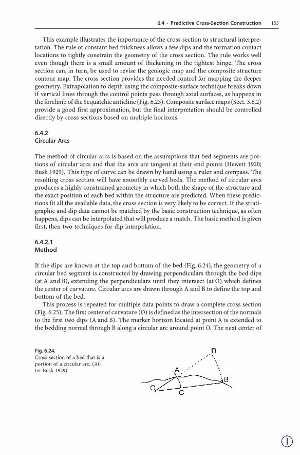
If the dips are known at the top and bottom of the bed (Fig. 6.24), the geometry of acircular bed segment is constructed by drawing perpendiculars through the bed dips(at A and B), extending the perpendiculars until they intersect (at O) which definesthe center of curvature. Circular arcs are drawn through A and B to define the top andbottom of the bed.

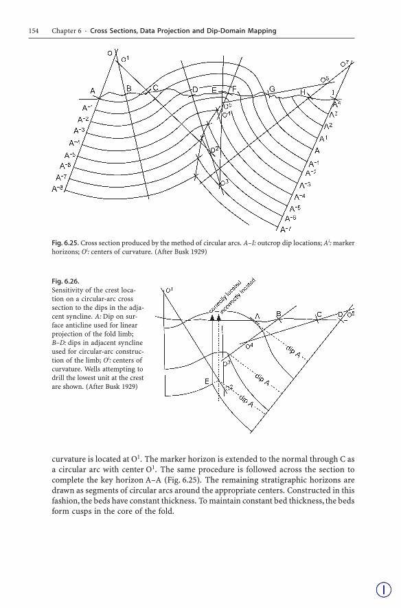
This process is repeated for multiple data points to draw a complete cross section(Fig. 6.25). The first center of curvature (O) is defined as the intersection of the normalsto the first two dips (A and B). The marker horizon located at point A is extended tothe bedding normal through B along a circular arc around point O. The next center of

Fig. 6.24.Cross section of a bed that is aportion of a circular arc. (Af-ter Busk 1929)



curvature is located at O1. The marker horizon is extended to the normal through C asa circular arc with center O1. The same procedure is followed across the section tocomplete the key horizon A–A (Fig. 6.25). The remaining stratigraphic horizons aredrawn as segments of circular arcs around the appropriate centers. Constructed in thisfashion, the beds have constant thickness. To maintain constant bed thickness, the bedsform cusps in the core of the fold.

Fig. 6.25. Cross section produced by the method of circular arcs. A–I: outcrop dip locations; Ai: markerhorizons; Oi: centers of curvature. (After Busk 1929)

Fig. 6.26.Sensitivity of the crest loca-tion on a circular-arc crosssection to the dips in the adja-cent syncline. A: Dip on sur-face anticline used for linearprojection of the fold limb;B–D: dips in adjacent synclineused for circular-arc construc-tion of the limb; Oi: centers ofcurvature. Wells attempting todrill the lowest unit at the crestare shown. (After Busk 1929)

155

To properly control the geometry of a cross section at depth, data may be needed at along distance laterally from the area of interest (Fig. 6.26). For example, in order to cor-rectly locate the crest of an anticline at depth, dips are needed from the adjacent synclines.If the last dip in the anticline (Fig. 6.26) was collected at A, then the steep limb of thestructure would be drawn with the long dashed lines and the crest on the lowest horizonwould be at the location of the incorrect well. Using the dips at B, C, and D, the structureis drawn with the solid lines, and the crest is found to be at E (Fig. 6.26). This is a generalproperty of cross-section geometry and also applies to dip-domain constructions.

6.4.2.2Dip Interpolation

Frequently the predicted geometry and the bed locations do not agree. The predictedlocation of horizon A (Fig. 6.27) on the opposite limb of the anticline is at B, but thathorizon may actually crop out at B' or B''. This result means that insufficient data areavailable to force a correct solution. It is necessary to modify the data or to interpolateintermediate dip values between A and B in order to make the horizon intersect thesection at B' or B''. Two methods of dip interpolation will be given; the first is to inter-polate a planar dip segment and the second is to interpolate an intermediate dip.

The simplest method is to insert a straight line segment (AY, Fig. 6.28) between thetwo arc segments that produce the disagreement. This method is usually successfuland provides an end-member solution. The procedure is from Higgins (1962):

Fig. 6.27.Cross section showing the mis-match between the predictedlocation of the key bed at Aand its mapped location (B' or B") at B. (After Busk 1929)

Fig. 6.28.Interpolation using a straightline with a circular arc. (AfterHiggins 1962)



1. Extend the dips at A and B so that they intersect at X.2. On AX locate point Y such that YX = XB.3. Bisect angle YXB. The bisector will intersect BC, the normal to B, at Ob.4. With center Ob and radius BOb, draw the arc from B to Y. This arc is tangent to AY,

the straight-line extension of the dip from A.

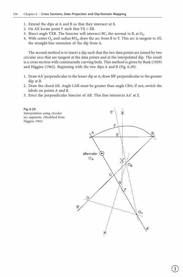
The second method is to insert a dip such that the two data points are joined by twocircular arcs that are tangent at the data points and at the interpolated dip. The resultis a cross section with continuously curving beds. This method is given by Busk (1929)and Higgins (1962). Beginning with the two dips A and B (Fig. 6.29):

1. Draw AA' perpendicular to the lesser dip at A; draw BB' perpendicular to the greaterdip at B.

2. Draw the chord AB. Angle CAB must be greater than angle CBA; if not, switch thelabels on points A and B.

3. Erect the perpendicular bisector of AB. This line intersects AA' at Z.

Fig. 6.29.Interpolation using circular-arc segments. (Modified fromHiggins 1962)

157

4. Choose point OA anywhere on line AA' on the opposite side of Z from A. (If the lengthOA–Z is very large, it is equivalent to drawing a straight line through A.)

5. On BB' locate point D such that BD = AOA.6. Draw DOA connecting D and OA.7. Erect the perpendicular bisector of DOA. This line intersects BB' at OB.8. Draw OAE' through OA and OB, intersecting AB at E.9. With center OA and radius AOA, draw an arc from A, intersecting OAE' at F.10.With center OB and radius BOB, draw an arc from B intersecting OAE' at F. This com-

pletes the interpolation.

If a correct solution is not obtained, it may be because the sense of curvature changesacross an inflection point, causing the centers of curvature to be on opposite sides ofthe key bed. Modify step 4 above by using the alternate position of OA (Fig. 6.29:alternate OA), located between C and A.

6.4.2.3Other Smooth Curves

Interactive computer drafting programs provide several different tools for drawingsmooth curves through or close to a specified set of points. Typically they are para-metric cubic curves for which the first derivatives, that is the tangents, are continuouswhere they join (Foley and Van Dam 1983). In this respect the curves are like themethod of circular arcs, for which the tangents are equal where the curve segmentsjoin, but cubics are able to fit more complex curves than just segments of circulararcs. Two different smooth curve types are widely available in interactive computerdrafting packages, Bézier and spline curves. The two curve types differ in how theyfit their control points and in how they are edited. Both types are useful in producingsmoothly curved lines and surfaces (Foley and Van Dam 1983; De Paor 1996).

A Bézier curve consists of segments that are defined by four control points,two anchor points on the curve (P1 and P4, Fig. 6.30a) and two direction points (P2and P3) that determine the shape of the curve. The curve always goes through theanchor points. The shape is controlled in interactive computer graphics applicationsby moving the direction points. In a computer program the direction points maybe connected to the anchors by lines to form handles (Fig. 6.30b) that are visible inthe edit mode. At the join between two Bézier segments, the handles of the sharedanchor point are colinear, ensuring that the slopes of the curve segments match at theintersection.

A spline curve only approximates the positions of its control points (Fig. 6.31) butis continuous in both the slope and the curvature at the segment boundaries, and sothe curve is even smoother than the Bézier curve (Foley and Van Dam 1983). Theshape is controlled in interactive computer graphics applications by moving the con-trol points that are visible in the edit mode. This curve type should be drawn sepa-rately from the actual data points because editing the curves changes the locations ofthe points that define the curve. The control points can be manipulated until the matchbetween the curve and the data points is acceptable.



Drawing a cross section (or a map) using the smooth curves just described requirescare to maintain the correct geometry. Constant bed thickness, for example, is not likelyto be maintained if the section is drawn from sparse data. The appropriate bed thick-ness relationships can be obtained by editing the curves after a preliminary section hasbeen drawn. The cross section of the Sequatchie anticline illustrates the problems. Theoriginal section (Fig. 6.23) was redrawn by changing the lines from polygons to splinecurves in a computer drafting program. The resulting cross section (Fig. 6.32) may bemore pleasing to the eye than the dip-domain cross section, but it is less accurate. Theunedited spline-curve version (Fig. 6.32a) is much too smooth. Each bedding surfaceis defined by 4 to 6 points, a data density that might be expected with control basedentirely on wells. Bedding thicknesses are not constant as in the dip-domain version,and the amplitude of the structure is reduced. These are the typical results of analyti-cal smoothing procedures, including the smoothing inherent in gridding as used formap construction. Editing the spline curves produces a better fit to the true dips(Fig. 6.32b). A more accurate spline section can be produced by introducing many morecontrol points, which is the appropriate procedure for producing a final drawing of aknown geometry. The addition of control points to improve an interpretation based ona sparse data set requires additional information, such as the bedding dips, or the re-quirement of constant bed thickness.

Fig. 6.31.Spline curve and its controlpoints

Fig. 6.30. Bézier curves. a The four control points that define the curve. b Two Bézier cubics joined atpoint P4. Points P3, P4, and P5 are colinear. (After Foley and Van Dam 1983)

159

6.5Changing the Dip of the Section Plane

If a cross section is not perpendicular to the fold axis, it is helpful for structural inter-pretation to rotate the section plane until it is a normal section. Alternatively, it mightbe necessary to rotate a normal section to vertical. The necessary relationships areequivalent to removing (or adding) a vertical exaggeration, as done in the visual methodof down-plunge viewing.

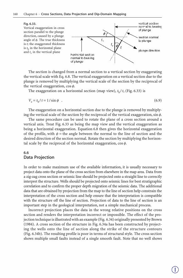
From the geometry of Fig. 6.33, the exaggeration in a vertical section across a plung-ing fold (Eq. 6.1) is

Ve = tv / t = 1 / cos φ . (6.8)

Fig. 6.32. Cross section of the Sequatchie anticline interpreted with spline curves. No vertical exag-geration. a Dip-domain cross section (thin solid lines from Fig. 6.23) and computer-smoothed splineinterpretation (thick dashed curves). b Spline curve section edited to more closely resemble the dip-domain section

6.5 · Changing the Dip of the Section Plane


The section is changed from a normal section to a vertical section by exaggeratingthe vertical scale with Eq. 6.8. The vertical exaggeration on a vertical section due to theplunge is removed by multiplying the vertical scale of the section by the reciprocal ofthe vertical exaggeration, cos φ.

The exaggeration on a horizontal section (map view), th / t, (Fig. 6.33) is

Ve = th/ t = 1 / sin φ . (6.9)

The exaggeration on a horizontal section due to the plunge is removed by multiply-ing the vertical scale of the section by the reciprocal of the vertical exaggeration, sin φ.

The same procedure can be used to rotate the plane of a cross section around avertical axis. Treat Fig. 6.33 as being the map view and the vertical exaggeration asbeing a horizontal exaggeration. Equation 6.8 then gives the horizontal exaggerationof the profile, with φ = the angle between the normal to the line of section and thedesired direction of the section normal. Rotate the section by multiplying the horizon-tal scale by the reciprocal of the horizontal exaggeration, cos φ.

6.6Data Projection

In order to make maximum use of the available information, it is usually necessary toproject data onto the plane of the cross section from elsewhere in the map area. Data froma zig-zag cross section or seismic line should be projected onto a straight line to correctlyinterpret the structure. Wells should be projected onto seismic lines for best stratigraphiccorrelation and to confirm the proper depth migration of the seismic data. The additionaldata that are obtained by projection from the map to the line of section help constrain theinterpretation of the cross section and help ensure that the interpretation is compatiblewith the structure off the line of section. Projection of data to the line of section is animportant step in the geological interpretation, not a simple mechanical process.

Incorrect projection places the data in the wrong relative positions on the crosssection and renders the interpretation incorrect or impossible. The effect of the pro-jection technique is illustrated with an example (Fig. 6.34) originally presented by Brown(1984). A cross section of the structure in Fig. 6.34a has been constructed by project-ing the wells onto the line of section along the strike of the structure contours(Fig. 6.34b). The resulting profile is poor in terms of structural style. The cross sectionshows multiple small faults instead of a single smooth fault. Note that no well shows

Fig. 6.33.Vertical exaggeration in crosssection parallel to the plungedirection, caused by a plungeangle of φ. The true thicknessis t; the exaggerated thicknessis th in the horizontal planeand tv in the vertical plane

161

more than one fault, yet the cross section shows locations where a vertical well shouldcut two faults. Projection along plunge (Fig. 6.34c) significantly improves the crosssection. The west half of the structure has a uniform cylindrical plunge to the west andso projection along plunge produces a reasonable cross section. Only one fault is presentand it is relatively planar, as expected.

Three general approaches to projection will be presented: projection along plunge,projection with a structure contour map, and projection within dip domains. For struc-tures where the plunge can be defined from bedding attitude data, projection alongplunge is effective. Where formation tops are relatively abundant, but attitudes are notavailable, projection by structure contouring is straightforward and accurate. Com-puter mapping programs usually take this approach. It must be recognized that thestructure contours themselves are interpretive and may not be correct in detail untilafter they have been checked on the cross section. Iterating between maps and thecross section in order to maintain the appropriate bed thicknesses is a powerful tech-nique for improving the interpretation of both the maps and the cross section. For dip-domain style structures, defining the dip-domain (axial-surface) network is an effi-cient method for projecting the geometry in three dimensions.

Fig. 6.34. Different cross sections obtained by different methods of data projection. a Structure con-tour map of horizon E, showing the alternative projection directions. Solid lines are parallel to the foldaxis; dashed lines are parallel to structure contours. b Cross section produced by projecting wells alongstructure contours. c Cross section produced by projecting wells along the plunge of the fold axis. SL sealevel. (After Brown 1984)

6.6 · Data Projection


Not all features in the same area will necessarily have the same projection direction.For example, stratigraphic thickness changes may be oblique to the structural trendsand should therefore be projected along a trend different from the structural trend.Folds and cross-cutting faults may have different projection directions. The respectivetrends and plunges should be determined from structure contour maps (Chap. 3), iso-pach maps (Sect. 4.3.1) and dip-sequence analysis (Chap. 9).

6.6.1Projection Along Plunge

Projection of information along plunge is most appropriate where the local data aretoo sparse to generate a structure contour map, but where the trend and plunge can bedetermined from bedding attitudes, for example, from a dipmeter.

6.6.1.1Projecting a Point or a Well

The projection of a point, such as a formation top in a well, along plunge to a newlocation, such as a vertical cross section or a seismic line (Fig. 6.35) is done using

v = h tan φ , (6.10)

where v = vertical elevation change, h = horizontal distance in the direction of plungefrom projection point to the cross section, and φ = plunge. For example, if h = 1 kmand the plunge is 15° (Fig. 6.35), the elevation of the projected point is 268 m lower onthe cross section than in the well.

6.6.1.2Plunge Lines

Projection along plunge is conveniently done using plunge lines, which are lines in theplunge direction, inclined at the plunge amount (Wilson 1967; De Paor 1988). Plunge lines

Fig. 6.35. Projection of a well along plunge to a cross section or seismic profile. a Map view of the projectionof the well to cross section A–A'. The arrow gives the plunge direction; φ plunge amount; h horizontal dis-tance in direction of plunge from projection point to cross section; v vertical elevation change. b 3-D view

163

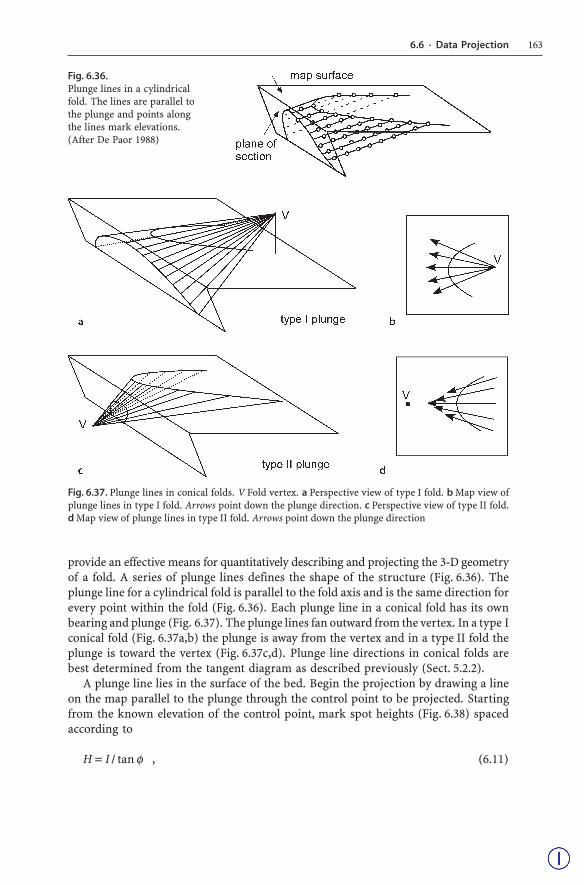
provide an effective means for quantitatively describing and projecting the 3-D geometryof a fold. A series of plunge lines defines the shape of the structure (Fig. 6.36). Theplunge line for a cylindrical fold is parallel to the fold axis and is the same direction forevery point within the fold (Fig. 6.36). Each plunge line in a conical fold has its ownbearing and plunge (Fig. 6.37). The plunge lines fan outward from the vertex. In a type Iconical fold (Fig. 6.37a,b) the plunge is away from the vertex and in a type II fold theplunge is toward the vertex (Fig. 6.37c,d). Plunge line directions in conical folds arebest determined from the tangent diagram as described previously (Sect. 5.2.2).

A plunge line lies in the surface of the bed. Begin the projection by drawing a lineon the map parallel to the plunge through the control point to be projected. Startingfrom the known elevation of the control point, mark spot heights (Fig. 6.38) spacedaccording to

H = I / tan φ , (6.11)

Fig. 6.36.Plunge lines in a cylindricalfold. The lines are parallel tothe plunge and points alongthe lines mark elevations.(After De Paor 1988)

Fig. 6.37. Plunge lines in conical folds. V Fold vertex. a Perspective view of type I fold. b Map view ofplunge lines in type I fold. Arrows point down the plunge direction. c Perspective view of type II fold.d Map view of plunge lines in type II fold. Arrows point down the plunge direction



where H = horizontal spacing of points, I = contour interval, and φ = plunge. If thecontrol point is not at a spot height, the distance from the control point to the first spotheight is

h' = H v' / I , (6.12)

where h' = the horizontal distance from the control point to the first spot height andv' = the elevation difference between the control point and the first spot height.

Projection along plunge lines is particularly suited to projecting data from an ir-regular surface, such as a map, onto a surface, such as a cross section or fault plane,that itself can be represented as a structure-contour map. Figure 6.39 shows plungelines derived from a map of a folded marker horizon on a topographic base. The fold

Fig. 6.38.Projection along plunge in avertical cross section. Theprojection is parallel to plungealong the plunge line frompoint 1 to point 2. Open circlesare spot heights along theplunge line. For explanationof symbols, see text

Fig. 6.39. Projection of a marker horizon to a fault plane along plunge lines. Dashed lines are topo-graphic contours above sea level. Dotted lines are subsurface structure contours on the fault. Plungelines are solid and marked by spot elevations. (After De Paor 1988)

165

is projected south, up plunge, along the plunge lines onto the structure contour mapof a fault. The intersection points where the plunge lines have the same elevation asthe fault contours are marked and then connected by a line that represents the traceof the marker horizon of the fault plane (Fig. 6.39). In 3-D (Fig. 6.40a), the outcroptrace is projected up and down plunge from the outcrop trace to more completelyillustrate the fold.

A structure contour map can be constructed from the plunge lines by joining thepoints of equal elevation (Fig. 6.40b). Figure 6.40b demonstrates that the plunge linesare not parallel to the structure contours and that projections should be made parallelto the plunge lines, not parallel to the structure contours. The structure contours pro-vide an additional cross check on the geometry of the structure and on the internalconsistency of the data. Once the fold geometry is constructed the plunge lines can bedeleted and the shape shown by structure contours alone (Fig. 6.40c).

This technique can be performed analytically using the method of De Paor (1988).An individual point P (Fig. 6.41), given by its xyz map coordinate position, can be pro-jected along plunge to its new position P' (x', 0, z') on the cross-section plane (definedby y' = 0). Select the map coordinate system such that x is parallel to the line of crosssection and y is perpendicular to the line of section. Choose y = z = 0 to lie in the plane

Fig. 6.40. 3-D views of the map in Fig. 6.39. a Oblique view to NW. Topographic surface with whitecontours, fault with thin black contours, fold with thick black plunge lines. b Vertical view, N up. Struc-ture contours (with elevations) and plunge lines on the fold, structure contours (with elevations) onlyon the fault. White line is outcrop trace of fold. c Oblique view to NW. Same as a except fold shapeindicated by structure contours



of the cross section. The sign convention requires that the positive (down) plungedirection be in the negative y direction. The elevation of a point is z. The dip of theplunge line = φ , the angle between the plunge line and the normal to the crosssection = α, and the dip of the cross section = δ . The plunge line is constant in direc-tion in a cylindrical fold but may be different for every location in a conical fold.

The general equations for the projected position of a point P', derived at the end ofthe chapter (Eqs. 6.36 and 6.41), are:

x' = x + y tan α + tan α (z cos α – y tan φ) / (tan φ + tan δ cos α) , (6.13)

z' = (z cos α – y tan φ) / (tan φ cos δ + sin δ cos α) . (6.14)

For a vertical cross section, from Eqs. 6.42 and 6.43,

x' = x + y tan α , (6.15)

z' = z – (y tan φ) / cos α . (6.16)

A cross section perpendicular to the fold axis is possible only for a cylindrical fold.The equations for projection to the normal section are (from Eqs. 6.44 and 6.45)

x' = x , (6.17)

z' = z cos φ – y sin φ . (6.18)

Fig. 6.41. Projection along plunge into the plane of the cross section. a Perspective diagram. b Horizontalmap projection. The projection of the section plane onto the map is shaded

167

In a conical fold the plunge amount and direction changes with location. A crosssection perpendicular to the crestal line will be closely equivalent to a normal sectionin slightly conical structures. Substitute the plunge of the crestal line in Eqs. 6.17 and6.18 to approximate a normal section. The shorter the projection distance, the betterthe approximation.

6.6.1.3Graphical Projection

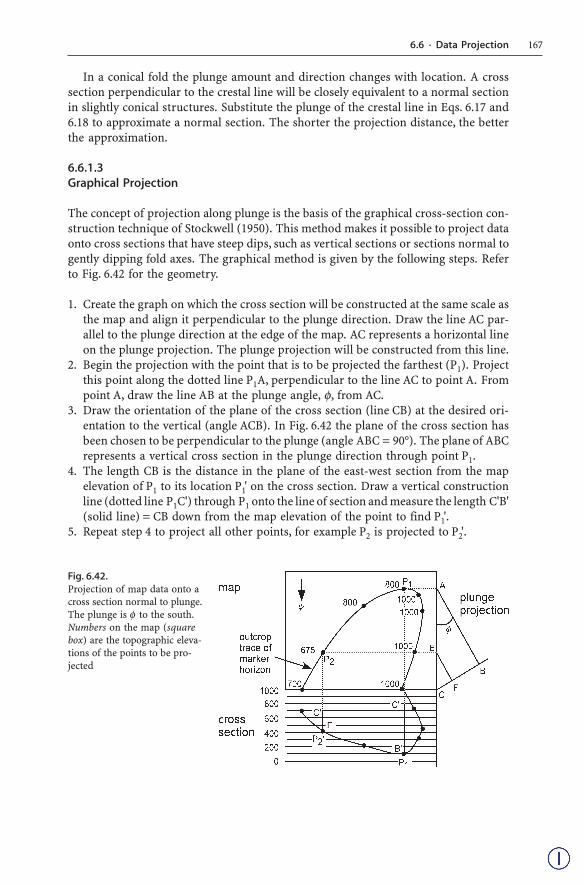
The concept of projection along plunge is the basis of the graphical cross-section con-struction technique of Stockwell (1950). This method makes it possible to project dataonto cross sections that have steep dips, such as vertical sections or sections normal togently dipping fold axes. The graphical method is given by the following steps. Referto Fig. 6.42 for the geometry.

1. Create the graph on which the cross section will be constructed at the same scale asthe map and align it perpendicular to the plunge direction. Draw the line AC par-allel to the plunge direction at the edge of the map. AC represents a horizontal lineon the plunge projection. The plunge projection will be constructed from this line.

2. Begin the projection with the point that is to be projected the farthest (P1). Projectthis point along the dotted line P1A, perpendicular to the line AC to point A. Frompoint A, draw the line AB at the plunge angle, φ, from AC.

3. Draw the orientation of the plane of the cross section (line CB) at the desired ori-entation to the vertical (angle ACB). In Fig. 6.42 the plane of the cross section hasbeen chosen to be perpendicular to the plunge (angle ABC = 90°). The plane of ABCrepresents a vertical cross section in the plunge direction through point P1.

4. The length CB is the distance in the plane of the east-west section from the mapelevation of P1 to its location P1' on the cross section. Draw a vertical constructionline (dotted line P1C') through P1 onto the line of section and measure the length C'B'(solid line) = CB down from the map elevation of the point to find P1'.

5. Repeat step 4 to project all other points, for example P2 is projected to P2'.

Fig. 6.42.Projection of map data onto across section normal to plunge.The plunge is φ to the south.Numbers on the map (squarebox) are the topographic eleva-tions of the points to be pro-jected



The ratio of the vertical projection length AB to the cross-section projection lengthCB is constant for all points, CB : CA = CF : CE = sin φ. Projection by hand is very rapidif a proportional divider drafting tool is used. Set the divider to the ratio CB / AB; thenas the projection length AC is set, the divider gives the required length CB.

The method can be modified for other cross-section orientations by changing theorientation of the line of section on the plunge projection (Fig. 6.43). The orientationof the plane of section on the plunge projection is CB. In Fig. 6.43, CB is at 90° to AC,making the section plane vertical. The ratio CB : CA is constant for all points. Followsteps 1 to 5 above, changing the orientation of the line CB.

The plunge of a fold typically changes along the axis. Cylindrical fold axes may becurved along the plunge and cylindrical folds will change into conical folds at theirterminations. Projection along straight plunge lines should be done only within do-mains for which the geometry of the structure is constant. Variable plunge can berecognized from undulations of the crest line on a structure-contour map or as exces-sive dispersion of the bedding dips around the best-fit curves on a stereogram or tan-gent diagram. If the plunge is variable, then the geographic size of the region beingutilized should be reduced until the plunge is constant and all the bedding points fitthe appropriate line on the stereogram or tangent diagram. If the sequence of plungeangle changes along the fold axis direction can be determined, then the straight line AB(Figs. 6.42, 6.43) could be replaced by a curved plunge line.

6.6.2Projection by Structure Contouring

Structure contours represent the position of a marker horizon or a fault between the controlpoints. Contouring provides a very general method for projecting data and can be usedwhere the plunge cannot be defined from attitude measurements. This is a convenientmethod in three-dimensional interpretation. The projection technique is to map the markersurfaces between control points and draw cross illustrative sections through the maps.

Fig. 6.43.Projection along plunge ontoa vertical cross section. Num-bers on the map (square box)are the topographic elevationsof the points to be projected

169

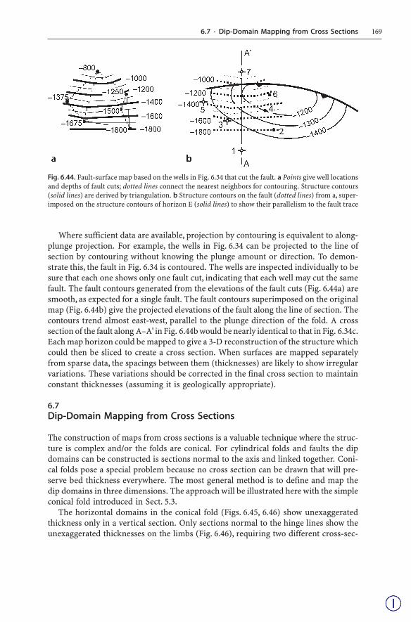
Where sufficient data are available, projection by contouring is equivalent to along-plunge projection. For example, the wells in Fig. 6.34 can be projected to the line ofsection by contouring without knowing the plunge amount or direction. To demon-strate this, the fault in Fig. 6.34 is contoured. The wells are inspected individually to besure that each one shows only one fault cut, indicating that each well may cut the samefault. The fault contours generated from the elevations of the fault cuts (Fig. 6.44a) aresmooth, as expected for a single fault. The fault contours superimposed on the originalmap (Fig. 6.44b) give the projected elevations of the fault along the line of section. Thecontours trend almost east-west, parallel to the plunge direction of the fold. A crosssection of the fault along A–A' in Fig. 6.44b would be nearly identical to that in Fig. 6.34c.Each map horizon could be mapped to give a 3-D reconstruction of the structure whichcould then be sliced to create a cross section. When surfaces are mapped separatelyfrom sparse data, the spacings between them (thicknesses) are likely to show irregularvariations. These variations should be corrected in the final cross section to maintainconstant thicknesses (assuming it is geologically appropriate).

6.7Dip-Domain Mapping from Cross Sections

The construction of maps from cross sections is a valuable technique where the struc-ture is complex and/or the folds are conical. For cylindrical folds and faults the dipdomains can be constructed is sections normal to the axis and linked together. Coni-cal folds pose a special problem because no cross section can be drawn that will pre-serve bed thickness everywhere. The most general method is to define and map thedip domains in three dimensions. The approach will be illustrated here with the simpleconical fold introduced in Sect. 5.3.

The horizontal domains in the conical fold (Figs. 6.45, 6.46) show unexaggeratedthickness only in a vertical section. Only sections normal to the hinge lines show theunexaggerated thicknesses on the limbs (Fig. 6.46), requiring two different cross-sec-

Fig. 6.44. Fault-surface map based on the wells in Fig. 6.34 that cut the fault. a Points give well locationsand depths of fault cuts; dotted lines connect the nearest neighbors for contouring. Structure contours(solid lines) are derived by triangulation. b Structure contours on the fault (dotted lines) from a, super-imposed on the structure contours of horizon E (solid lines) to show their parallelism to the fault trace

6.7 · Dip-Domain Mapping from Cross Sections


tion trends (110° and 250°). In the region of the 11° south plunge, a section normal toplunge is normal to bedding (Fig. 6.46) but will give an exaggerated thickness wherebeds are horizontal.

The simplest procedure is to map axial surfaces on straight, vertical cross sections(Fig. 6.47), or from multiple map horizons. An axial surface is by definition the surfacethrough successive hinge lines. This relationship applies regardless of whether or notthe profile is perpendicular to the bedding or to the hinge lines. Axial surfaces onsuccessive cross sections are correlated and then mapped in 3-D (Fig. 6.48a). Axialsurfaces in conical folds will intersect in three dimensions, and the intersection linesmust be located (Fig. 6.48b). Once the axial surfaces and their intersections are con-structed, the marker horizons can be mapped across the region (Fig. 6.49). Because adip domain is a region of uniform dip, once the domain boundaries have been located,bedding attitudes may be projected anywhere within a single domain. Bedding sur-faces can be projected throughout the entire domain from a single observation point.

Fig. 6.45. Dip domains in conical fold. a Dip-domain map of middle horizon. b Structure contour mapof middle horizon showing lines of cross section (heavy EW lines)

Fig. 6.46.Tangent diagram of conicalfold in Fig. 6.45 showing thedirections of the 3 sectionlines that preserve bed thick-ness in local areas. In the norththe fold crest is horizontal, andin the south it plunges 11, 180

171

Some types of information, for example fracture density, may be related to the prox-imity of the observation point to the fold hinge and so should be projected parallel tothe closest hinge line. 3-D axial surface maps provide essential information for pre-dicting the deep structure using kinematic models of cross-section geometry (espe-cially using flexural-slip models Sect. 11.6).

Fig. 6.47.Axial surface traces definedon a vertical slice oblique tohinge lines (northern sectionacross Fig. 6.45b); ast: axialsurface trace; hp: hinge point

Fig. 6.48. Axial surfaces in the fold of Fig. 6.45. a Constructed by linking traces on profiles. b Completedaxial surface network superimposed on previous construction

Fig. 6.49. Completed marker surfaces for map in Fig. 6.45. a Top. b Middle. c Bottom

6.7 · Dip-Domain Mapping from Cross Sections


6.8Derivations


From Fig. 6.50a, the dip of a marker on an unexaggerated profile is

tan δ = v / h , (6.19)

and the thickness of a unit in terms of its vertical dimension is

t = L sin (90 – δ) = L cos δ , (6.20)

where δ = unexaggerated dip, t = unexaggerated thickness, and L = unexaggeratedvertical thickness. Let the vertical exaggeration be Ve = vv / v and the horizontal exag-geration be He = hh / h, where v and h are the original horizontal and vertical scalesand the subscripts h and v indicate the exaggerated scale. The equations for the exag-gerated dips (Fig. 6.50b) have the same form as Eq. 6.19:

Fig. 6.50. Horizontal and vertical exaggeration. a Unexaggerated cross section. b Exaggerated horizontalscale; horizontal exaggeration (He) = 2 : 1. c Exaggerated vertical scale; vertical exaggeration (Ve) = 2 : 1

173

tan δv = vv / h , (6.21a)

tan δh = v / hh . (6.21b)

Replace h in Eq. 6.21a and v in 6.21b with the values from Eq. 6.19 and use the defini-tion of the exaggeration to obtain the relationship between original and exaggerated dips:

tan δv = Ve tan δ , (6.22a)

tan δh = tan δ / He . (6.22b)

To relate the horizontal to the vertical exaggeration, substitute the value of tan δfrom Eq. 6.22a into 6.22b to obtain

Ve He = tan δv / tan δh . (6.23)

To obtain the same exaggerated angle by either horizontal or vertical exaggeration,set δv = δh in Eq. 6.23:

Ve = 1 / He . (6.24)

The thickness of a unit on a horizontally exaggerated profile (Fig. 6.50b), th, is

sin (90 – δh) = cos δh = th / L . (6.25)

Eliminate L by dividing Eq. 6.25 by 6.20:

th / t = cos δh/ cos δ . (6.26)

The thickness of a unit on a vertically exaggerated profile (Fig. 6.50c), tv, is

cos δv = tv / (Ve L) . (6.27)

Eliminate L by dividing Eq. 6.27 by Eq. 6.20:

tv / t = Ve (cos δv / cos δ) . (6.28)

6.8.2Analytical Projection along Plunge Lines

The point P is to be projected parallel to plunge to point P' on the cross section(Fig. 6.51a). The plunge direction makes an angle of α to the direction of the perpen-dicular to the cross section (Fig. 6.51d) and the plunge is φ. Following the method ofDe Paor (1988), the x coordinate axis is taken parallel to the line of the section and theplane of section intersects the x axis at zero elevation. In the plane of the cross section,

6.8 · Derivations


the position of point P (x, y, z) is P' (x', z'). The apparent dip of the intersection line, q,of the vertical plane through PP' with the cross section is δ '. The relationship betweenthe apparent dip and the true dip, δ, of the z' line, is given by Eq. 2.18 as

tan δ ' = tan δ cos α . (6.29)

Begin by finding z'. In the plane normal to the cross section (Fig. 6.51a,c),

z' = OP' / sin δ . (6.30)

In the plane of the plunge (Fig. 6.51b), using triangles AQP' and PQR,

OP' = q sin δ ' , (6.31)

∆z = L tan φ , (6.32)

Fig. 6.51.Projection along plunge. a Per-spective diagram. b Verticalplane through plunge line PP'.c Vertical plane normal to thecross section through line OP'.d Plan view. Projection of thecross section is shaded. Point Qis vertically above A at A–Q andpoint P' is vertically above Oat O–P'

175

v = z – L tan φ , (6.33)

and by using the law of sines with angles AQP' and QP'A in triangle QAP', along withcos φ = sin (90 – φ),

q = v / (tan φ cos δ ' + sin δ ') . (6.34)

In the plane of the map (Fig. 6.51d)

L = y / cos α . (6.35)

Substitute Eqs. 6.29, 6.31, 6.33, 6.34 and 6.35 into 6.30 to obtain

z' = (z cos α – y tan φ) / (tan φ cos δ + sin δ cos α) . (6.36)

The x' coordinate is found from (Fig. 6.51a)

x' = x + ∆x + b . (6.37)

In the plane of the map (Fig. 6.51d)

∆x = y tan α , (6.38)

b = OB tan α . (6.39)

In the plane normal to the cross section (Fig. 6.51c)

OB = OP' / tan δ . (6.40)

Substitute Eqs. 6.29, 6.31–6.35 and 6.38–6.40, into 6.37 to obtain

x' = x + y tan α + tan α (z cos α – y tan φ) / (tan φ + tan δ cos α) . (6.41)

For a vertical cross section, δ = 90° and Eqs. 6.36 and 6.41 reduce to

x' = x + y tan α , (6.42)

z' = z – y tan φ / cos α . (6.43)

For a cross section normal to the plunge line, possible only for a cylindrical fold,α = 0, δ = (90 – φ) and Eqs. 6.36 and 6.41 reduce to

x' = x , (6.44)

z' = z cos φ – y sin φ . (6.45)

6.8 · Derivations


6.9Exercises


Draw the cross section in Fig. 6.52 vertically exaggerated by a factor of 5 : 1. Draw thecross section in Fig. 6.52 horizontally squeezed by a factor of 1 : 2.

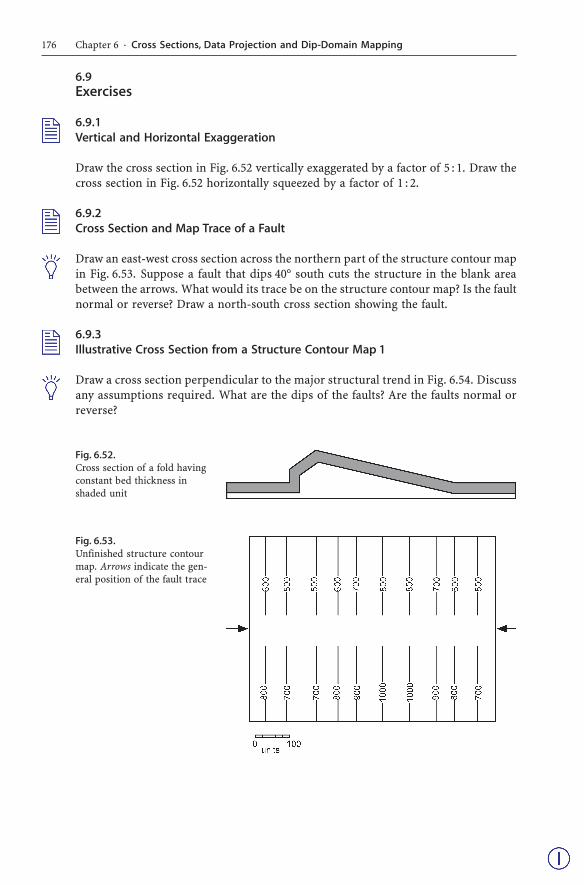
6.9.2Cross Section and Map Trace of a Fault

Draw an east-west cross section across the northern part of the structure contour mapin Fig. 6.53. Suppose a fault that dips 40° south cuts the structure in the blank areabetween the arrows. What would its trace be on the structure contour map? Is the faultnormal or reverse? Draw a north-south cross section showing the fault.

6.9.3Illustrative Cross Section from a Structure Contour Map 1

Draw a cross section perpendicular to the major structural trend in Fig. 6.54. Discussany assumptions required. What are the dips of the faults? Are the faults normal orreverse?

Fig. 6.52.Cross section of a fold havingconstant bed thickness inshaded unit

Fig. 6.53.Unfinished structure contourmap. Arrows indicate the gen-eral position of the fault trace

177


Draw cross sections along the three lines indicated on Fig. 6.55. Using the fault dipdetermined from the map, extend the faults above and below the marker horizon untilthey intersect. Which fault(s) formed last?


Draw cross sections along the three lines indicated in Fig. 6.56. Determine the dips ofthe faults from the map and then extend the faults above and below the marker hori-zon until they intersect. Which fault is youngest?

6.9.6Predictive Dip-Domain Section

Complete the cross section in Fig. 6.57 by extending it into the air and deeper into thesubsurface. How far can the section be realistically extended?

Fig. 6.54.Structure contour map of thetop of the Gwin coal cycle.Elevations of the top Gwin areposted next to the wells. Unitsare in feet, negative below sealevel

6.9 · Exercises


Fig. 6.56.Structure contour map of areverse-faulted surface. Thehorizon surface is repeated bythe fault zones. The fault cut-offs are wider lines. Hiddencontours are dashed. The loca-tions of lines of section A–A',B–B', and C–C' are shown

Fig. 6.57.Partially complete dip-domaincross section. Dashed lines areaxial-surface traces

Fig. 6.55.Structure contour map of anormal-faulted surface. Thehorizon surface is missing inthe shaded fault zones. Loca-tions of lines of section A–A',B–B', and C–C' are shown

179

6.9.7Predictive Cross Sections from Bedding Attitudes and Tops

Complete the cross section in Fig. 6.58, keeping bed thicknesses constant. Use both thedip-domain technique and the method of circular arcs. Scan the section into a com-puter and complete using the smooth curves provided by a drafting program. Com-pare the results of the different techniques.

6.9.8Fold and Thrust Fault Interpretation

Construct illustrative cross section A–A' from the map in Fig. 3.29 using the struc-ture contour map constructed in Exercise 3.7.4. Use the dip-domain technique toconstruct the same cross section using only the surface geology along the profile. Usethe circular arc technique to construct the same cross section using only the sur-face geology along the profile. What is the plunge of the central portion of the struc-ture from a stereogram or tangent diagram? Project the northern part of the struc-ture onto section B–B' using the method of along-plunge projection. Compare andcontrast the cross sections. The wells to the Fairholme were drilled to find a hydro-carbon trap but were not successful. Use the map and cross sections to determine astructural reason for drilling the wells and a structural reason that they were unsuc-cessful.

6.9.9Projection

Project the top reservoir onto the seismic line assuming the structure is normal to theseismic line (Fig. 6.59). Project the top reservoir onto the seismic line assuming thestructure plunges 10° in the direction 225°.

Fig. 6.58. Cross section through the Burma No. 1 and 2 wells. Short lines are surface dips. Letters A–Gare marker horizons seen at the locations of dip measurements that can be correlated. Arrows point tolocations where markers can be identified in outcrop but the dip cannot be measured. The dips in thewells are from oriented cores

6.9 · Exercises


Fig. 6.59.Map showing trace of a seismicline and the location of a well

Documents

Cross Sections, Data Projection and Dip -Domain Mappingextras.springer.com/2006/978-3-540-31054-9/Data/006.pdf · 134 Chapter 6 · Cross Sections, Data Projection and Dip-Domain Mapping