Embed Size (px)
Citation preview

Cross-Shore Sediment Transport Processes III-3-i
Chapter 3CROSS-SHORE SEDIMENT EM 1110-2-1100TRANSPORT PROCESSES (Part III)
1 August 2008 (Change 2)
Table of Contents
Page
III-3-1. Introduction . . . . . . . . . . . . . . . . . . . . . . . . . . . . . . . . . . . . . . . . . . . . . . . . . . . . . . . . . . . . III-3-1a. Overview/purpose . . . . . . . . . . . . . . . . . . . . . . . . . . . . . . . . . . . . . . . . . . . . . . . . . . . . . . III-3-1b. Scope of chapter . . . . . . . . . . . . . . . . . . . . . . . . . . . . . . . . . . . . . . . . . . . . . . . . . . . . . . . III-3-2
III-3-2. General Characteristics of Natural and Altered Profiles . . . . . . . . . . . . . . . . . . . . III-3-2a. Forces acting in the nearshore . . . . . . . . . . . . . . . . . . . . . . . . . . . . . . . . . . . . . . . . . . . . III-3-2b. Equilibrium beach profile characteristics . . . . . . . . . . . . . . . . . . . . . . . . . . . . . . . . . . . . III-3-9c. Interaction of structures with cross-shore sediment transport . . . . . . . . . . . . . . . . . . . III-3-16d. Methods of measuring beach profiles . . . . . . . . . . . . . . . . . . . . . . . . . . . . . . . . . . . . . . III-3-16
(1) Introduction . . . . . . . . . . . . . . . . . . . . . . . . . . . . . . . . . . . . . . . . . . . . . . . . . . . . . . . III-3-16(a) Fathometer . . . . . . . . . . . . . . . . . . . . . . . . . . . . . . . . . . . . . . . . . . . . . . . . . . . . . III-3-16(b) CRAB . . . . . . . . . . . . . . . . . . . . . . . . . . . . . . . . . . . . . . . . . . . . . . . . . . . . . . . . . III-3-18(c) Sea sled . . . . . . . . . . . . . . . . . . . . . . . . . . . . . . . . . . . . . . . . . . . . . . . . . . . . . . . III-3-19(d) Hydrostatic profiler . . . . . . . . . . . . . . . . . . . . . . . . . . . . . . . . . . . . . . . . . . . . . . III-3-19
(2) Summary . . . . . . . . . . . . . . . . . . . . . . . . . . . . . . . . . . . . . . . . . . . . . . . . . . . . . . . . . III-3-19
III-3-3. Engineering Aspects of Beach Profiles and Cross-shore Sediment Transport . . . . . . . . . . . . . . . . . . . . . . . . . . . . . . . . . . . . . . . . . . . . . . . . . . . . . . . . . . . III-3-19a. Introduction . . . . . . . . . . . . . . . . . . . . . . . . . . . . . . . . . . . . . . . . . . . . . . . . . . . . . . . . . . III-3-19b. Limits of cross-shore sand transport in the onshore and offshore directions . . . . . . . . III-3-19c. Quantitative description of equilibrium beach profiles . . . . . . . . . . . . . . . . . . . . . . . . . III-3-21d. Computation of equilibrium beach profiles . . . . . . . . . . . . . . . . . . . . . . . . . . . . . . . . . . III-3-25e. Application of equilibrium profile methods to nourished beaches. . . . . . . . . . . . . . . . . III-3-25f. Quantitative relationships for nourished profiles . . . . . . . . . . . . . . . . . . . . . . . . . . . . . III-3-26g. Longshore bar formation and seasonal shoreline changes . . . . . . . . . . . . . . . . . . . . . . III-3-32h. Static models for shoreline response to sea level rise and/or storm effects . . . . . . . . . III-3-43i. Computational models for dynamic response to storm effects . . . . . . . . . . . . . . . . . . . . III-3-51
(1) Introduction . . . . . . . . . . . . . . . . . . . . . . . . . . . . . . . . . . . . . . . . . . . . . . . . . . . . . . . III-3-51(2) Numerical and analytical models . . . . . . . . . . . . . . . . . . . . . . . . . . . . . . . . . . . . . . . III-3-51(3) General description of numerical models . . . . . . . . . . . . . . . . . . . . . . . . . . . . . . . . . III-3-52
(a) Conservation equation . . . . . . . . . . . . . . . . . . . . . . . . . . . . . . . . . . . . . . . . . . . . III-3-52(b) Transport relationships . . . . . . . . . . . . . . . . . . . . . . . . . . . . . . . . . . . . . . . . . . . . III-3-52(c) Closed loop transport relationships . . . . . . . . . . . . . . . . . . . . . . . . . . . . . . . . . . III-3-52(d) Open loop transport relationships . . . . . . . . . . . . . . . . . . . . . . . . . . . . . . . . . . . III-3-52
(4) General description of analytical models . . . . . . . . . . . . . . . . . . . . . . . . . . . . . . . . . III-3-54j. Example application of an analytical model . . . . . . . . . . . . . . . . . . . . . . . . . . . . . . . . . III-3-55k. Examples of numerical models . . . . . . . . . . . . . . . . . . . . . . . . . . . . . . . . . . . . . . . . . . . III-3-59l. Physical modeling of beach profile response . . . . . . . . . . . . . . . . . . . . . . . . . . . . . . . . . III-3-65

EM 1110-2-1100 (Part III)1 Aug 08 (Change 2)
III-3-ii Cross-Shore Sediment Transport Processes
III-3-4. References . . . . . . . . . . . . . . . . . . . . . . . . . . . . . . . . . . . . . . . . . . . . . . . . . . . . . . . . . . . III-3-69
III-3-5. Definition of Symbols . . . . . . . . . . . . . . . . . . . . . . . . . . . . . . . . . . . . . . . . . . . . . . . . . . III-3-76
III-3-6. Acknowledgments . . . . . . . . . . . . . . . . . . . . . . . . . . . . . . . . . . . . . . . . . . . . . . . . . . . . . III-3-79
EM 1110-2-1100 (Part III)1 Aug 08 (Change 2)
Cross-Shore Sediment Transport Processes III-3-iii
List of Tables
Page
Table III-3-1Constructive and Destructive Cross-shore “Forces” in Terms of Induced Bottom Shear Stresses . III-3-11
Table III-3-2Summary of Field Evaluation of Various Nearshore Survey Systems (Based on Clausner, Birkemeier, and Clark (1986)) . . . . . . . . . . . . . . . . . . . . . . . . . . . . . . . . . . . . . . . . . . . . . . . . . . III-3-18
Table III-3-3Summary of Recommended A Values (Units of A Parameter are m1/3) . . . . . . . . . . . . . . . . . . . . . . III-3-24

EM 1110-2-1100 (Part III)1 Aug 08 (Change 2)
III-3-iv Cross-Shore Sediment Transport Processes
List of Figures
Page
Figure III-3-1. Longshore (qx) and cross-shore (qy) sediment transport components . . . . . . . . III-3-1
Figure III-3-2. Problems and processes in which cross-shore sediment transport isrelevant . . . . . . . . . . . . . . . . . . . . . . . . . . . . . . . . . . . . . . . . . . . . . . . . . . . . . . . III-3-3
Figure III-3-3. Definition sketch . . . . . . . . . . . . . . . . . . . . . . . . . . . . . . . . . . . . . . . . . . . . . . . . III-3-4
Figure III-3-4. Variation with time of the bottom shear stress under a breaking nonlinearwave. H = 0.78 m, h= 1.0 m, T = 8.0 s, and D = 0.2 mm . . . . . . . . . . . . . . . . . III-3-5
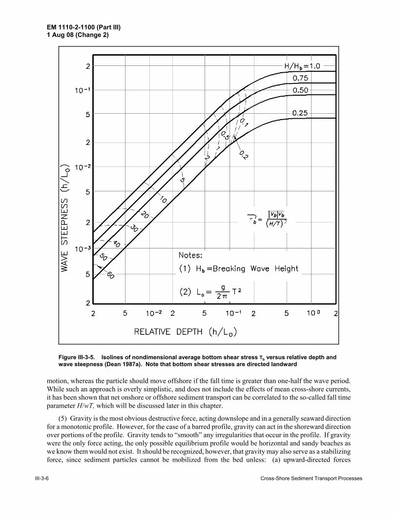
Figure III-3-5. Isolines of nondimensional average bottom shear stress Jb versusrelative depth and wave steepness (Dean 1987a). Note that bottomshear stresses are directed landward. . . . . . . . . . . . . . . . . . . . . . . . . . . . . . . . . . III-3-6
Figure III-3-6. Distribution over depth of the flux of the onshore component ofmomentum . . . . . . . . . . . . . . . . . . . . . . . . . . . . . . . . . . . . . . . . . . . . . . . . . . . . . III-3-8
Figure III-3-7. Bottom stresses caused by surface winds . . . . . . . . . . . . . . . . . . . . . . . . . . . . . III-3-8
Figure III-3-8. Velocity distributions inside and outside the surf zone for nosurface wind stress and cases of no overtopping and full overtop-ping both inside and outside the surf zone . . . . . . . . . . . . . . . . . . . . . . . . . . . III-3-10
Figure III-3-9. Effects of varying wave energy flux (a) on: (b) shoreline position,and (c) foreshore beach slope (dots are shoreline position in (b) and(c), solid curve is trend line in (b), foreshore slope in (c)) (Katohand Yanagishima 1988) . . . . . . . . . . . . . . . . . . . . . . . . . . . . . . . . . . . . . . . . . . III-3-12
Figure III-3-10. Examples of two offshore bar profiles . . . . . . . . . . . . . . . . . . . . . . . . . . . . . . III-3-13
Figure III-3-11. Variation in shoreline and bar crest positions, Duck, NC (Lee andBirkemeier 1993) . . . . . . . . . . . . . . . . . . . . . . . . . . . . . . . . . . . . . . . . . . . . . . . III-3-14
Figure III-3-12. Definition of offshore bar characteristics (Keulegan 1945) . . . . . . . . . . . . . . III-3-15
Figure III-3-13. Nondimensional geometries of natural bars compared with thoseproduced in the laboratory (Keulegan 1948) . . . . . . . . . . . . . . . . . . . . . . . . . . III-3-15
Figure III-3-14. Profiles extending across the continental shelf for three locationsalong the East and Gulf coastlines of the United States (Dean1987a) . . . . . . . . . . . . . . . . . . . . . . . . . . . . . . . . . . . . . . . . . . . . . . . . . . . . . . . III-3-17
Figure III-3-15. Comparison of response of natural and seawalled profiles toHurricane Elena, September, 1985 (Kriebel 1987) . . . . . . . . . . . . . . . . . . . . III-3-18

EM 1110-2-1100 (Part III)1 Aug 08 (Change 2)
Cross-Shore Sediment Transport Processes III-3-v
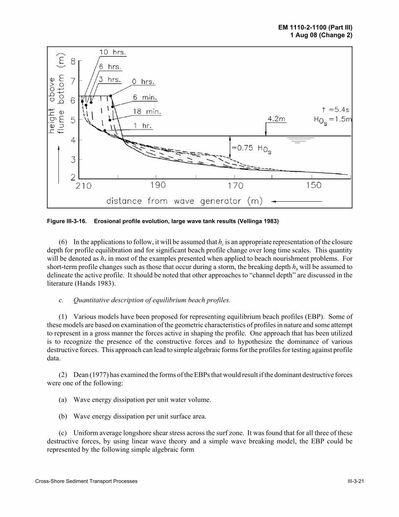
Figure III-3-16. Erosional profile evolution, large wave tank results (Vellinga 1983) . . . . . . . III-3-21
Figure III-3-17. Variation of sediment scale parameter A with sediment size D andfall velocity wf (Dean 1987b) . . . . . . . . . . . . . . . . . . . . . . . . . . . . . . . . . . . . . III-3-23
Figure III-3-18. Variation of sediment scale parameter A(D) with sediment size Dfor beach sand sizes . . . . . . . . . . . . . . . . . . . . . . . . . . . . . . . . . . . . . . . . . . . . . III-3-23
Figure III-3-19. Equilibrium beach profiles for sand sizes of 0.3 mm and 0.6 mmA(D = 0.3 mm) = 0.12 m1/3, A(D = 0.6 mm) =0.20 m1/3 . . . . . . . . . . . . . . . . . III-3-26
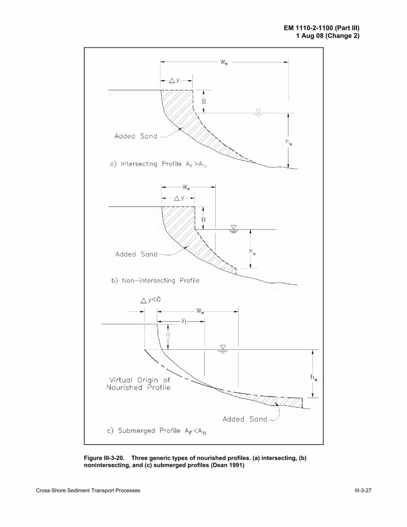
Figure III-3-20. Three generic types of nourished profiles (a) intersecting, (b) non-intersecting, and (c) submerged profiles (Dean 1991) . . . . . . . . . . . . . . . . . . III-3-27
Figure III-3-21. Effect of nourishment material scale parameter AF on width ofresulting dry beach. Four examples of decreasing AF with sameadded volume per unit beach length (Dean 1991) . . . . . . . . . . . . . . . . . . . . . . III-3-28
Figure III-3-22. Effect of increasing volume of sand added on resulting beachprofile. AF = 0.1 m1/3, AN = 0.2 m1/3, h* = 6.0 m, B = 1.5 m (Dean1991) . . . . . . . . . . . . . . . . . . . . . . . . . . . . . . . . . . . . . . . . . . . . . . . . . . . . . . . . III-3-29
Figure III-3-23. (1) Volumetric requirement for finite shoreline advancement(Equation 3-23); (2) Volumetric requirement for intersectingprofiles (Equation 3-22). Results presented for special case BN =0.25 . . . . . . . . . . . . . . . . . . . . . . . . . . . . . . . . . . . . . . . . . . . . . . . . . . . . . . . . . III-3-31
Figure III-3-24. Variation of nondimensional shoreline advancement )y/W*, withAN and V. Results shown for h*/B = 2.0 (BN=0.5) (Dean 1991) . . . . . . . . . . . III-3-33
Figure III-3-25. Variation of nondimensional shoreline advancement )y/W*, withAN and V. Results shown for h*/B = 3.0 (BN= 0.333) (Dean 1991) . . . . . . . . . III-3-34
Figure III-3-26. Variation of nondimensional shoreline advancement )y/W*, withAN and V. Results shown for h*/B = 4.0 (BN=0.25) (Dean 1991) . . . . . . . . . . III-3-35
Figure III-3-27. Nourishment with coarser sand than native (Intersecting profiles) . . . . . . . . III-3-37
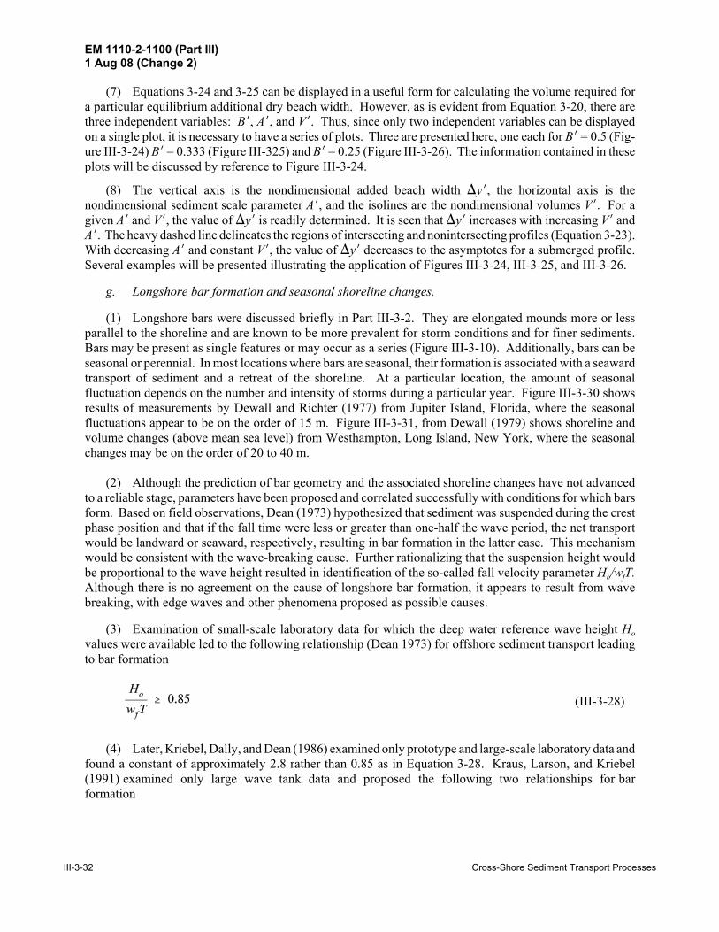
Figure III-3-28. Example III-3-3. Nourishment with same-sized sand as native(Nonintersecting profiles) . . . . . . . . . . . . . . . . . . . . . . . . . . . . . . . . . . . . . . . . III-3-39
Figure III-3-29. Illustration of effect of volume added V and fill sediment scaleparameter AF on additional dry beach width )y. Example condi-tions: B = 1.5 m,h* = 6 m,AN = 0.1 m1/3 . . . . . . . . . . . . . . . . . . . . . . . . . . . . . . III-3-40
Figure III-3-30. Mean monthly shoreline position A and unit volume B at Jupiter,referenced to first survey (Dewall and Richter 1977) . . . . . . . . . . . . . . . . . . . III-3-41
Figure III-3-31. Changes in shoreline position and unit volume at WesthamptonBeach, New York (Dewall 1979) . . . . . . . . . . . . . . . . . . . . . . . . . . . . . . . . . . III-3-42
EM 1110-2-1100 (Part III)1 Aug 08 (Change 2)
III-3-vi Cross-Shore Sediment Transport Processes
Figure III-3-32. Components of sand volume balance due to sea level rise andassociated profile retreat according to the Bruun Rule . . . . . . . . . . . . . . . . . . III-3-44
Figure III-3-33. The Bruun Rule generalized for the case of a barrier island thatmaintains its form relative to the adjacent ocean and lagoon (Deanand Maurmeyer 1983) . . . . . . . . . . . . . . . . . . . . . . . . . . . . . . . . . . . . . . . . . . . III-3-45
Figure III-3-34. Elements of the Edelman model . . . . . . . . . . . . . . . . . . . . . . . . . . . . . . . . . . . III-3-46
Figure III-3-35. Profile forms considered by Kriebel and Dean (1993) . . . . . . . . . . . . . . . . . . III-3-48
Figure III-3-36. Two types of grids employed in numerical modelling of cross-shore sediment transport and profile evolution . . . . . . . . . . . . . . . . . . . . . . . . III-3-53
Figure III-3-37. Examples of profile response to idealized sine-squared storm surge:(a) Short-duration hurricane, and (b) Long-duration northeaster(Kriebel and Dean 1993) . . . . . . . . . . . . . . . . . . . . . . . . . . . . . . . . . . . . . . . . . III-3-56
Figure III-3-38. Maximum relative erosion versus ratio of storm duration to profiletime scale TD/TS . . . . . . . . . . . . . . . . . . . . . . . . . . . . . . . . . . . . . . . . . . . . . . . . III-3-57
Figure III-3-39. Empirical relationship for determination of erosion time scale Ts . . . . . . . . . III-3-57
Figure III-3-40. Potential and actual shoreline response based on Kriebel and Dean(1993) model . . . . . . . . . . . . . . . . . . . . . . . . . . . . . . . . . . . . . . . . . . . . . . . . . . III-3-59
Figure III-3-41. Kriebel and Dean erosion model calibration using large-wave tankdata of Saville (1957) (from Kriebel (1990)) . . . . . . . . . . . . . . . . . . . . . . . . . III-3-61
Figure III-3-42. Comparison of Kriebel and Dean erosion model to measuredprofiles from northeast storm at Point Pleasant, NJ (from Kriebel(1990)). . . . . . . . . . . . . . . . . . . . . . . . . . . . . . . . . . . . . . . . . . . . . . . . . . . . . . . III-3-61
Figure III-3-43. SBEACH compared to two tests from large-scale wave tanks(Larson and Kraus 1989) . . . . . . . . . . . . . . . . . . . . . . . . . . . . . . . . . . . . . . . . . III-3-63
Figure III-3-44. SBEACH tested against profile evolution data from Duck, NC(Larson and Kraus 1989) . . . . . . . . . . . . . . . . . . . . . . . . . . . . . . . . . . . . . . . . . III-3-64
Figure III-3-45. Noda's recommendation for profile modeling (Noda 1972) . . . . . . . . . . . . . . III-3-66
Figure III-3-46. Profile evolution by small- and large-scale wave tank tests. Basedon maintaining the same fall velocity parameter. Length ratio =1:9.6 (Kriebel, Dally, and Dean 1986) . . . . . . . . . . . . . . . . . . . . . . . . . . . . . . III-3-68
Figure III-3-47. Profile evolution by small- and large-scale wave tank tests. Case ofsloping seawall. Based on maintaining the same fall velocityparameter. Length ratio = 1:7.5 (Hughes and Fowler 1990) . . . . . . . . . . . . . III-3-69

EM 1110-2-1100 (Part III)1 Aug 08 (Change 2)
Cross-Shore Sediment Transport Processes III-3-1
Figure III-3-1. Longshore (qx) and cross-shore (qy) sedimenttransport components
Chapter III-3Cross-Shore Sediment Transport Processes
III-3-1. Introduction
a. Overview/purpose.
(1) Sediment transport at a point in the nearshore zone is a vector with both longshore and cross-shorecomponents (see Figure III-3-1). It appears that under a number of coastal engineering scenarios of interest,transport is dominated by either the longshore or cross-shore component and this, in part, has led to a historyof separate investigative efforts for each of these two components. The subject of total longshore sedimenttransport has been studied for approximately five decades. There is still considerable uncertainty regardingcertain aspects of this transport component including the effects of grain size, barred topography, and thecross-shore distribution of longshore transport. A focus on cross-shore sediment transport is relatively recent,having commenced approximately one decade ago and uncertainty in prediction capability (including theeffects of all variables) may be considerably greater. In some cases the limitations on prediction accuracyof both components may be due as much to a lack of good wave data as to an inadequate understanding oftransport processes.
(2) Cross-shore sediment transport encompasses both offshore transport, such as occurs during storms,and onshore transport, which dominates during mild wave activity. Transport in these two directions appearsto occur in significantly distinct modes and with markedly disparate time scales; as a result, the difficultiesin predictive capabilities differ substantially. Offshore transport is the simpler of the two and tends to occur

EM 1110-2-1100 (Part III)1 Aug 08 (Change 2)
III-3-2 Cross-Shore Sediment Transport Processes
with greater rapidity and as a more regular process with transport more or less in phase over the entire activeprofile. This is fortunate since there is considerably greater engineering relevance and interest in offshoretransport due to the potential for damage to structures and loss of land. Onshore sediment transport withinthe region delineated by the offshore bar often occurs in “wave-like” motions referred to as“ridge-and-runnel” systems in which individual packets of sand move toward, merge onto, and widen the drybeach. A complete understanding of cross-shore sediment transport is complicated by the contributions ofboth bed and suspended load transport. Partitioning between the two components depends in an unknownway on grain size, local wave energy, and other variables.
(3) Cross-shore sediment transport is relevant to a number of coastal engineering problems, including:(a) beach and dune response to storms, (b) the equilibration of a beach nourishment project that is placed atslopes steeper than equilibrium, (c) so-called “profile nourishment” in which the sand is placed in thenearshore with the expectation that it will move landward nourishing the beach (this involves the moredifficult problem of onshore transport), (d) shoreline response to sea level rise, (e) seasonal changes ofshoreline positions, which can amount to 30 to 40 m, (f) overwash, the process of landward transport due toovertopping of the normal land mass due to high tides and waves, (g) scour immediately seaward of shore-parallel structures, and (h) the three-dimensional flow of sand around coastal structures in which the steeperand milder slopes on the updrift and downdrift sides of the structure induce seaward and landwardcomponents, respectively. These problems are schematized in Figure III-3-2.
b. Scope of chapter.
(1) This chapter consists of two additional sections. The first section describes the general characteristicsof equilibrium beach profiles and cross-shore sediment transport. This section commences with a qualitativedescription of the forces acting within the nearshore zone, the characteristics of an equilibrium beach profile,and a discussion of conditions of equilibrium when the forces are balanced, as well as the ensuing sedimenttransport when conditions change, causing an imbalance. The general profile characteristics across thecontinental shelf are reviewed with special emphasis on the more active nearshore zone. Bar morphologyand short- and long-term changes of beach profiles due to storms and sea level rise are examined, along witheffects of various parameters on the profile characteristics, including wave climate and sedimentcharacteristics. Survey capabilities to quantify the profiles are reviewed.
(2) The second section deals with quantitative aspects of cross-shore sediment transport with specialemphasis on engineering applications and the prediction of beach profile change. First, the general shape ofthe equilibrium beach profile is quantified in terms of sediment grain size and basic wave parameters.Equilibrium profile methods are then used to develop analytical solutions to several problems of interest inbeach nourishment design. Similar analytical solutions are developed for the steady-state beach profileresponse to elevated water levels, including both the long-term response to sea level rise and the short-termresponse to storm surge. For simplified cases, analytical methods are then presented for estimating thedynamic profile response during storms. For more general applications, numerical modelling approaches arerequired and these are briefly reviewed.
III-3-2. General Characteristics of Natural and Altered Profiles
a. Forces acting in the nearshore.
(1) There are several identifiable forces that occur within the nearshore active zone that affect sedimentmotion and beach profile response. The magnitudes of these forces can be markedly different inside and

EM 1110-2-1100 (Part III)1 Aug 08 (Change 2)
Cross-Shore Sediment Transport Processes III-3-3
Figure III-3-2. Problems and processes in which cross-shore sediment transport is relevant

EM 1110-2-1100 (Part III)1 Aug 08 (Change 2)
III-3-4 Cross-Shore Sediment Transport Processes
(III-3-1)
Figure III-3-3. Definition sketch
(III-3-2)
outside the surf zone. Under equilibrium conditions, these forces are in balance and although there is motionof the individual sand grains under even low wave activity, the profile remains more or less static. Cross-shore sediment transport occurs when hydrodynamic conditions within the nearshore zone change, therebymodifying one or more of the forces resulting in an imbalance and thus causing transport gradients and profilechange. Established terminology is that onshore- and offshore-directed forces are referred to as “construc-tive” and “destructive,” respectively. These two types of forces are briefly reviewed below; however, as willbe noted, the term “forces” is used in the generic sense. Moreover it will be evident that some forces couldbehave as constructive under certain conditions and destructive under others.
(2) As noted, constructive forces are those that tend to cause onshore sediment transport. For classicnonlinear wave theories (Stokes, Cnoidal, Solitary, Stream Function, etc.), the wave crests are higher and ofshorter duration than are the troughs. This feature is most pronounced just outside the breaking point and alsoapplies to the water particle velocities. For oscillatory water particle velocities expressed as a sum of phase-locked sinusoids such as for the Stokes or Stream Function wave theories, even though the time mean of thewater particle velocity is zero, the average of the bottom shear stress Jb expressed as
can be shown to be directed onshore. In the above, D is the mass density of water, f is the Darcy-Weisbachfriction coefficient which, for purposes here is considered constant over a wave period, and vb is theinstantaneous wave-induced water particle velocity at the bottom. A definition sketch is provided in Fig-ure III-3-3. An example of the time-varying shear stress due to a nonlinear (Stream Function) wave is shownin Figure III-3-4. Dean (1987a) has developed the average bottom shear stress based on the Stream Functionwave theory and presented the results in the nondimensional form shown in Figure III-3-5.
(3) A second constructive force originates within the bottom boundary layer, causing a net mean velocityin the direction of propagating water waves. This streaming motion was first observed in the laboratory byBagnold (1940) and has been quantified by Longuet-Higgins (1953) as due to the local transfer of momentumassociated with energy losses by friction. For the case of laminar flows, the maximum (over depth) value ofthis steady velocity vs is surprisingly independent of the value of the viscosity and is given by
EM 1110-2-1100 (Part III)1 Aug 08 (Change 2)
Cross-Shore Sediment Transport Processes III-3-5
Figure III-3-4. Variation with time of the bottom shear stress under a breakingnonlinear wave. H = 0.78 m, h= 1.0 m, T = 8.0 s, and D = 0.2 mm
(III-3-3)
which, for the case of shallow water and a wave height proportional to the breaking depth, will be shown tobe 1.5 times the average of the return flow due to the mass transport. In Equation 3-2, F is the wave angularfrequency, k is the wave number, and H the wave height. Although the maximum velocity is independentof the viscosity, the bottom shear stress Jbs induced by the streaming velocity is not and is given by
in which , is the eddy viscosity.
(4) Within the surf zone, cross-shore transport may be predominantly due to sediment in suspension.If the suspension is intermittent, occurring each wave period, the average water particle velocity during theperiod that the particle is suspended determines the direction of cross-shore transport. Although this causeof sediment transport is not a true force, it does represent a contributing mechanism. Turbulence, althoughalso not a true force, can be effective in mobilizing sediment and dependent on whether the net forces areshoreward or seaward at the time of mobilization, can be constructive or destructive, respectively. Dean(1973) noted that suspended sediment can move either onshore (constructive) or offshore (destructive),depending on how high a sand grain is suspended off the bottom. Under the wave crest, if the sedimentparticle is suspended a distance above the bottom proportional to the wave height H, and if the particle hasa fall velocity w, then the time required for the grain to fall back to the bottom would be proportional to H/w.If this fall time is less than one-half of the wave period, then the particle should experience net onshore
EM 1110-2-1100 (Part III)1 Aug 08 (Change 2)
III-3-6 Cross-Shore Sediment Transport Processes
Figure III-3-5. Isolines of nondimensional average bottom shear stress Jb versus relative depth andwave steepness (Dean 1987a). Note that bottom shear stresses are directed landward
motion, whereas the particle should move offshore if the fall time is greater than one-half the wave period.While such an approach is overly simplistic, and does not include the effects of mean cross-shore currents,it has been shown that net onshore or offshore sediment transport can be correlated to the so-called fall timeparameter H/wT, which will be discussed later in this chapter.
(5) Gravity is the most obvious destructive force, acting downslope and in a generally seaward directionfor a monotonic profile. However, for the case of a barred profile, gravity can act in the shoreward directionover portions of the profile. Gravity tends to “smooth” any irregularities that occur in the profile. If gravitywere the only force acting, the only possible equilibrium profile would be horizontal and sandy beaches aswe know them would not exist. It should be recognized, however, that gravity may also serve as a stabilizingforce, since sediment particles cannot be mobilized from the bed unless: (a) upward-directed forces

EM 1110-2-1100 (Part III)1 Aug 08 (Change 2)
Cross-Shore Sediment Transport Processes III-3-7
(III-3-4)
(III-3-5)
associated with fluid turbulence can exceed the submerged weight of the sediment, and/or (b) slope-parallelfluid shear forces can exceed the frictional resistance of sediment. Also, as noted, gravity causes suspendedsediment to settle out of the water column, with fall velocity w, which may cause suspended sediment to moveshoreward if not suspended too high in the water column.
(6) Other destructive forces are generally related to the vertical structure of the cross-shore currents. Theundertow, the seaward return flow of wave mass transport, induces a seaward stress on the bottom sedimentparticles. For linear waves, the time-averaged seaward discharge due to the return flow of shoreward masstransport Q is (Dean and Dalrymple 1991)
where E is the wave energy density and C is the wave celerity. If the return flow due to mass transport weredistributed uniformly over the water depth, it can be shown from linear shallow-water wave theory that themean velocity would be
which, as noted for shallow water, is two-thirds of the maximum streaming velocity. Within the surf zone,the wave height can be considered to be proportional to the local depth, as H = 6 h, so that the mean velocityfurther simplifies to 0.08 (gh)1/2 for 6 . 0.78 where (gh)1/2 is the wave celerity in shallow water. In stormevents where there is overtopping of the barrier island, a portion or all of the potential return flow due to masstransport can be relieved through strong landward flows, thereby eliminating this destructive force andresulting instead in constructive forces.
(7) It is well-known that associated with wave propagation toward shore is a shoreward flux of linearmomentum (Longuet-Higgins and Stewart 1964). When waves break, the momentum is transferred to thewater column, resulting in a shoreward-directed thrust and thus a wave-induced setup within the surf zone,the gradient of which is proportional to the local bottom slope. This momentum is distributed over depth,as shown in Figure III-3-6. In shallow water, linear water wave theory predicts that one-third of themomentum flux originates between the trough and crest levels and has its centroid at the mean water level.The remaining two-thirds originates between the bottom and the mean water level, is uniformly distributedover this dimension, and thus has its centroid at the mid-depth of the water column. Because of thecontribution at the free surface, breaking waves induce an equivalent shear force on the water surface whichwill be quantified later. This causes a seaward bottom shear stress within the breaking zone. The bottomshear stress is dependent on the rate of energy dissipation. This effective shear force due to momentumtransfer must be balanced by the bottom shear stress and the pressure forces due to the slope of the watersurface.
(8) Often during major storm events, strong onshore winds will be present in the vicinity of the shoreline.These winds cause a shoreward-directed surface flow and a seaward-directed bottom flow, as shown in Fig-ure III-3-7. Of course, seaward-directed winds would cause shoreward-directed bottom velocities and thusconstructive forces. Thus, landward- and seaward-directed winds result in destructive and constructive forces,respectively.

EM 1110-2-1100 (Part III)1 Aug 08 (Change 2)
III-3-8 Cross-Shore Sediment Transport Processes
Figure III-3-6. Distribution over depth of the flux of the onshore component ofmomentum
Figure III-3-7. Bottom stresses caused by surface winds
(9) Considering linear wave theory, and a linear shear stress relationship with eddy viscosity ,, thedistribution of the mean velocity over depth for the case of return of mass transport (no overtopping) andwithout including the contribution of bottom streaming can be shown to be (Dean and Dalrymple 2000)
(III-3-6)
In this expression, the first term is associated with the surface wind stress J0. The second term is associatedwith the vertical gradient of momentum flux and is expressed as a function of the cross-shore gradient in waveenergy ME/My. It is noted that this term is zero outside the breakpoint and contributes only inside the surf zonewhere energy is dissipated. The third term is associated with the seaward return flow of mass transport, whereQ represents the net seaward discharge over the water column as given by Equation 3-4.
(10) For the three effects considered in Equation 3-6, the shear stress associated with the vertical velocitydistribution may be computed for any elevation z as
EM 1110-2-1100 (Part III)1 Aug 08 (Change 2)
Cross-Shore Sediment Transport Processes III-3-9
(III-3-7)
(III-3-8)
where , is the turbulent eddy viscosity. The resulting seaward-directed shear stress at the bottom (z = -h) isthen given by
(11) Velocity distributions and shear stress distributions inside and outside the surf zone based on Equa-tions III-3-6 and III-3-7 are shown in Figure III-3-8 for a condition of no surface wind stress and for casesof no overtopping and full overtopping both inside and outside the breakpoint. Profile conditions assumedfor this example are shown in the figure caption and assume an equilibrium beach profile where wavebreaking is assumed to occur at a depth of 1 m. For the case with no overtopping, most of the seawardvelocity shown in Figure III-3-8 is due to the return flow required to balance the shoreward flows near thesurface. This is further illustrated in the cases with overtopping where it is assumed that the shoreward flowsovertop the profile so that there is no net return flow due to mass transport.
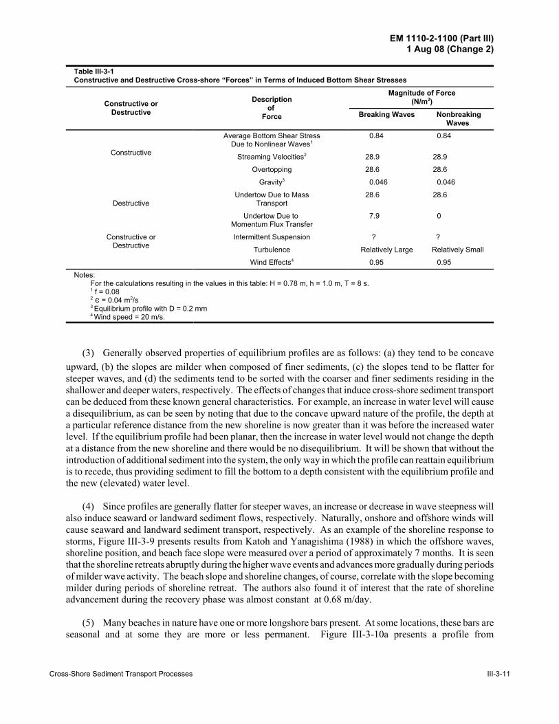
(12) Table III-3-1 summarizes the mechanisms identified as contributing to constructive and/ordestructive forces and, where possible, provides an estimate of their magnitudes. For purposes of thesecalculations, the following conditions have been considered: an equilibrium beach profile with a grain sizeof D = 0.2 mm, h = 1 m, H = 0.78 m, T = 8 s, , = 0.04 m2/s, wind speed = 20 m/s. It is seen that of the bottomstresses that can be quantified, those associated with undertow due to mass transport and momentum fluxtransfer are dominant.
b. Equilibrium beach profile characteristics.
(1) In considerations of cross-shore sediment transport, it is useful to first examine the case ofequilibrium in which there is no net cross-shore sediment transport. The competing forces elucidated in theprevious section can be fairly substantial, exerting tendencies for both onshore and offshore transport. Achange will bring about a disequilibrium that causes cross-shore sediment transport. The concept of anequilibrium beach profile has been criticized, since in nature the forces affecting equilibrium are alwayschanging with the varying tides, waves, currents, and winds. Although this is true, the concept of anequilibrium profile is one of the coastal engineer's most valuable tools in providing a framework to considerdisequilibrium and thus cross-shore sediment transport. Also, many useful and powerful conceptual anddesign relationships are based on profiles of equilibrium.
(2) When applying equilibrium profile concepts to problems requiring an estimate of profile retreat oradvance, a related concept of importance is the principle of conservation of sand across the profile. Underconditions where no longshore gradients exist in the longshore transport, onshore-offshore transport causesa redistribution of sand across the profile but does not lead to net gain or loss of sediment. Most engineeringmethods applied to the prediction of profile change ensure that the total sand volume is conserved in theactive profile, so that erosion of the exposed beach face requires a compensating deposition offshore, whiledeposition on the exposed beach face must be accompanied by erosion of sediment in the surf zone. For caseswhere longshore gradients in longshore transport do exist, it is then common to assume that the profile

EM 1110-2-1100 (Part III)1 Aug 08 (Change 2)
III-3-10 Cross-Shore Sediment Transport Processes
Figure III-3-8. Velocity distributions inside and outside the surf zone for no surface wind stress and casesof no overtopping and full overtopping both inside and outside the surf zone
advances or retreats uniformly at all active elevations while maintaining its shape across the profile. In thisway, sediment volume can be added or removed from the profile without changing the shape of the activeprofile. As a result, most methods for predicting beach profile change treat the longshore and cross-shorecomponents separately so that the final profile form and location are determined by superposition.
EM 1110-2-1100 (Part III)1 Aug 08 (Change 2)
Cross-Shore Sediment Transport Processes III-3-11
Table III-3-1Constructive and Destructive Cross-shore “Forces” in Terms of Induced Bottom Shear Stresses
Constructive orDestructive
Descriptionof
Force
Magnitude of Force(N/m2)
Breaking Waves NonbreakingWaves
Constructive
Average Bottom Shear StressDue to Nonlinear Waves1
0.84 0.84
Streaming Velocities2 28.9 28.9
Overtopping 28.6 28.6
Destructive
Gravity3 0.046 0.046
Undertow Due to MassTransport
28.6 28.6
Undertow Due to Momentum Flux Transfer
7.9 0
Constructive orDestructive
Intermittent Suspension ? ?
Turbulence Relatively Large Relatively Small
Wind Effects4 0.95 0.95
Notes:For the calculations resulting in the values in this table: H = 0.78 m, h = 1.0 m, T = 8 s.1 f = 0.082 , = 0.04 m2/s3 Equilibrium profile with D = 0.2 mm4 Wind speed = 20 m/s.
(3) Generally observed properties of equilibrium profiles are as follows: (a) they tend to be concaveupward, (b) the slopes are milder when composed of finer sediments, (c) the slopes tend to be flatter forsteeper waves, and (d) the sediments tend to be sorted with the coarser and finer sediments residing in theshallower and deeper waters, respectively. The effects of changes that induce cross-shore sediment transportcan be deduced from these known general characteristics. For example, an increase in water level will causea disequilibrium, as can be seen by noting that due to the concave upward nature of the profile, the depth ata particular reference distance from the new shoreline is now greater than it was before the increased waterlevel. If the equilibrium profile had been planar, then the increase in water level would not change the depthat a distance from the new shoreline and there would be no disequilibrium. It will be shown that without theintroduction of additional sediment into the system, the only way in which the profile can reattain equilibriumis to recede, thus providing sediment to fill the bottom to a depth consistent with the equilibrium profile andthe new (elevated) water level.
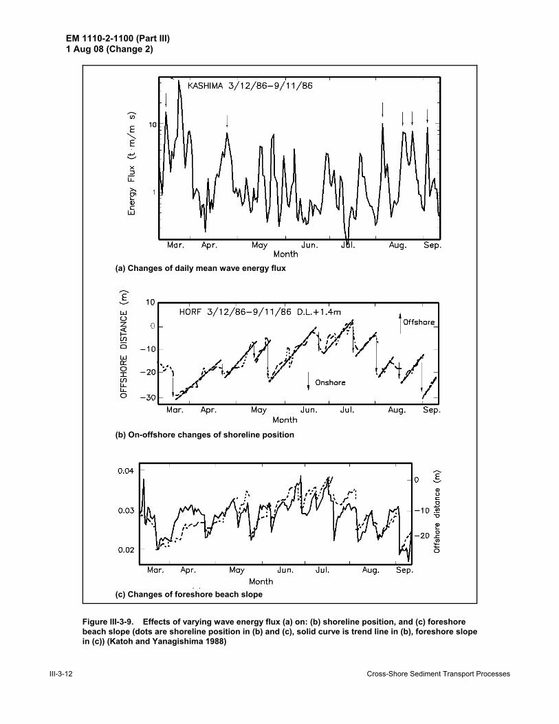
(4) Since profiles are generally flatter for steeper waves, an increase or decrease in wave steepness willalso induce seaward or landward sediment flows, respectively. Naturally, onshore and offshore winds willcause seaward and landward sediment transport, respectively. As an example of the shoreline response tostorms, Figure III-3-9 presents results from Katoh and Yanagishima (1988) in which the offshore waves,shoreline position, and beach face slope were measured over a period of approximately 7 months. It is seenthat the shoreline retreats abruptly during the higher wave events and advances more gradually during periodsof milder wave activity. The beach slope and shoreline changes, of course, correlate with the slope becomingmilder during periods of shoreline retreat. The authors also found it of interest that the rate of shorelineadvancement during the recovery phase was almost constant at 0.68 m/day.
(5) Many beaches in nature have one or more longshore bars present. At some locations, these bars areseasonal and at some they are more or less permanent. Figure III-3-10a presents a profile from
EM 1110-2-1100 (Part III)1 Aug 08 (Change 2)
III-3-12 Cross-Shore Sediment Transport Processes
(a) Changes of daily mean wave energy flux
(b) On-offshore changes of shoreline position
(c) Changes of foreshore beach slope
Figure III-3-9. Effects of varying wave energy flux (a) on: (b) shoreline position, and (c) foreshorebeach slope (dots are shoreline position in (b) and (c), solid curve is trend line in (b), foreshore slopein (c)) (Katoh and Yanagishima 1988)

EM 1110-2-1100 (Part III)1 Aug 08 (Change 2)
Cross-Shore Sediment Transport Processes III-3-13
(a) Multiple-barred Profile from Chesapeake Bay (from Dolan and Dean 1985)
(b) Profiles from Monitoring of a Beach and Profile Nourishment Project at PerdidoKey, FL
Figure III-3-10. Examples of two offshore bar profiles
Chesapeake Bay in which at least six bars are evident and Figure III-3-10b shows profiles measured in amonitoring program to document the evolution of a beach nourishment project at Perdido Key, FL. Thisproject included both beach nourishment in the form of a large seaward buildup of the berm and foreshoreand profile nourishment in the form of a large offshore mound. As seen from Figure III-3-10b, a bar waspresent before nourishment and gradually re-formed in depths of less than 1 m as the profile equilibratedduring the 2-year period shown in Figure III-3-10b.
(6) It will be shown later that the presence of bars depends on wave and sediment conditions and at aparticular beach, bars may form or move farther seaward during storms. It appears that the outer bars on someprofiles are relict and may have been caused by a past large storm which deposited the sand in water too deep
EM 1110-2-1100 (Part III)1 Aug 08 (Change 2)
III-3-14 Cross-Shore Sediment Transport Processes
Figure III-3-11. Variation in shoreline and bar crest positions, Duck, NC (Lee and Birkemeier 1993)
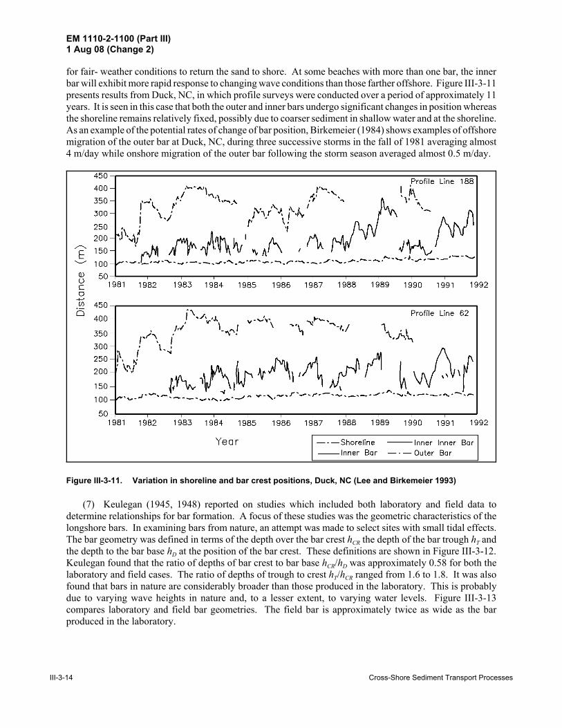
for fair- weather conditions to return the sand to shore. At some beaches with more than one bar, the innerbar will exhibit more rapid response to changing wave conditions than those farther offshore. Figure III-3-11presents results from Duck, NC, in which profile surveys were conducted over a period of approximately 11years. It is seen in this case that both the outer and inner bars undergo significant changes in position whereasthe shoreline remains relatively fixed, possibly due to coarser sediment in shallow water and at the shoreline.As an example of the potential rates of change of bar position, Birkemeier (1984) shows examples of offshoremigration of the outer bar at Duck, NC, during three successive storms in the fall of 1981 averaging almost4 m/day while onshore migration of the outer bar following the storm season averaged almost 0.5 m/day.
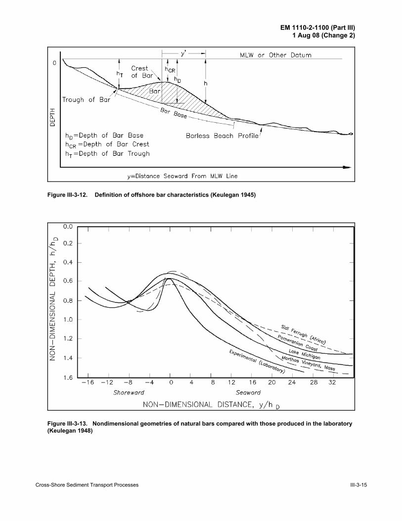
(7) Keulegan (1945, 1948) reported on studies which included both laboratory and field data todetermine relationships for bar formation. A focus of these studies was the geometric characteristics of thelongshore bars. In examining bars from nature, an attempt was made to select sites with small tidal effects.The bar geometry was defined in terms of the depth over the bar crest hCR the depth of the bar trough hT andthe depth to the bar base hD at the position of the bar crest. These definitions are shown in Figure III-3-12.Keulegan found that the ratio of depths of bar crest to bar base hCR/hD was approximately 0.58 for both thelaboratory and field cases. The ratio of depths of trough to crest hT/hCR ranged from 1.6 to 1.8. It was alsofound that bars in nature are considerably broader than those produced in the laboratory. This is probablydue to varying wave heights in nature and, to a lesser extent, to varying water levels. Figure III-3-13compares laboratory and field bar geometries. The field bar is approximately twice as wide as the barproduced in the laboratory.
EM 1110-2-1100 (Part III)1 Aug 08 (Change 2)
Cross-Shore Sediment Transport Processes III-3-15
Figure III-3-12. Definition of offshore bar characteristics (Keulegan 1945)
Figure III-3-13. Nondimensional geometries of natural bars compared with those produced in the laboratory(Keulegan 1948)

EM 1110-2-1100 (Part III)1 Aug 08 (Change 2)
III-3-16 Cross-Shore Sediment Transport Processes
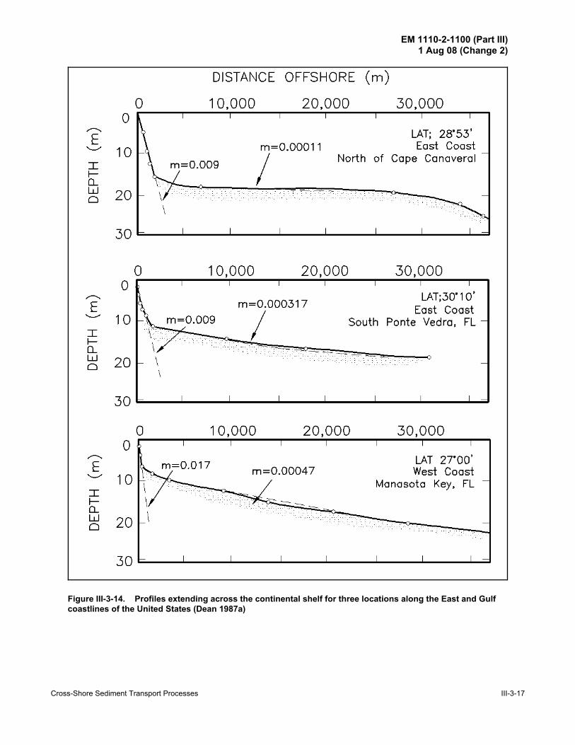
(8) The shapes of profiles across the continental shelf are less predictable than those within the moreactive zone of generally greater engineering interest. This may be due to the presence of bottom materialdifferent than sand (including rock and peat outcrops), the much greater time constants required for equilibra-tion in these greater depths, the greater role of currents in shaping the profile and the effects of past sea levelvariations. In general, the slopes seaward of the more active zone are quite small if the bottom is composedof sand or smaller-sized materials. Figure III-3-14 presents three examples of profiles extending off the Eastand Gulf coasts of Florida. It is seen that at this scale, the profile may be approximated by a nearshore slopethat extends to 5 to 18 m and milder seaward slopes, which are on the order of 1/2,000 to 1/10,000.
c. Interaction of structures with cross-shore sediment transport.
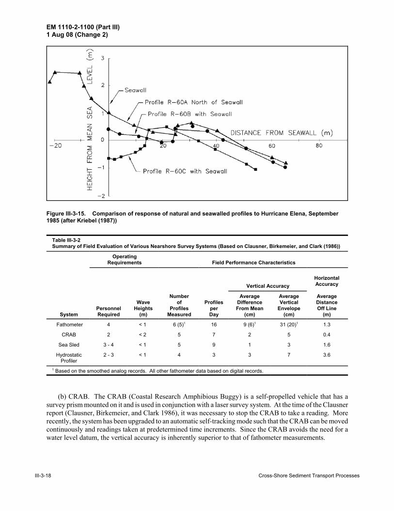
The structure that interacts most frequently with cross-shore sediment transport is a shore-parallelstructure such as a seawall or revetment. During storm events, a characteristic profile fronting a shore-parallelstructure is one with a trough at its base, as shown in Figure III-3-15, from Kriebel (1987) for a profileaffected by Hurricane Elena in Pinellas County, Florida, in September 1985. This trough is due to largetransport gradients immediately seaward of the structure. Although the hydrodynamic cause of this scour isnot well-known, it has been suggested that it is due to a standing wave system with an antinode at thestructure. A second, more heuristic explanation is that sand removal is prevented behind the seawall and thetransport system removes sand from as near as possible to where removal would normally occur. Barnett andWang (1988) have reported on a model study to evaluate the interaction of a seawall with the profile and havefound that the additional volume represented by the scour trough is approximately 62 percent of what wouldhave been removed landward of the seawall if it had not been present. During mild wave activity, it appearsthat the profile recovers nearly as it would have if the seawall had not been present. The reader is referredto the comprehensive review by Kraus (1988) for additional information on shore-parallel structures and theireffects on the shoreline.
d. Methods of measuring beach profiles.
(1) Introduction. Changes in beach and nearshore profiles are a result of cross-shore and longshoresediment transport. If the longshore gradients in the longshore component can be considered small, it ispossible, through the continuity equation, to infer the volumetric cross-shore transport from two successiveprofile surveys.
(2) Clausner, Birkemeier, and Clark (1986) have carried out a comprehensive field test of four nearshoresurvey systems, including: (a) the standard fathometer system, (b) the CRAB, which is aself-propelled platform on which a survey prism is mounted, (c) a sea sled, which also carries a prism but istowed by a boat or a cable from shore, and (d) a hydrostatic profiler, which utilizes a cable for towing andan oil-filled tube to sense the elevation difference between the shore and the location of the point beingsurveyed. Each of these systems is reviewed briefly below and their performance characteristics are describedand summarized in Table III-3-2.
(a) Fathometer. This method of measuring nearshore profiles requires knowledge of the water level asa reference datum. To provide a complete description of the active profile, fathometer surveys must becomplemented with surveys of the shallow-water and above-water portions of the profile. In the field tests,the fathometer was mounted on a 47-ft vessel and the surveys were conducted under favorable waveconditions, which should result in a lower estimate of the error. Characteristics of this system and resultsobtained from the field measurements are presented in Table III-3-2.
EM 1110-2-1100 (Part III)1 Aug 08 (Change 2)
Cross-Shore Sediment Transport Processes III-3-17
Figure III-3-14. Profiles extending across the continental shelf for three locations along the East and Gulfcoastlines of the United States (Dean 1987a)
EM 1110-2-1100 (Part III)1 Aug 08 (Change 2)
III-3-18 Cross-Shore Sediment Transport Processes
Figure III-3-15. Comparison of response of natural and seawalled profiles to Hurricane Elena, September1985 (after Kriebel (1987))
Table III-3-2Summary of Field Evaluation of Various Nearshore Survey Systems (Based on Clausner, Birkemeier, and Clark (1986))
System
OperatingRequirements Field Performance Characteristics
PersonnelRequired
WaveHeights
(m)
Numberof
ProfilesMeasured
ProfilesperDay
Vertical AccuracyHorizontalAccuracy
AverageDistanceOff Line
(m)
AverageDifferenceFrom Mean
(cm)
AverageVertical
Envelope(cm)
Fathometer 4 < 1 6 (5)1 16 9 (6)1 31 (20)1 1.3
CRAB 2 < 2 5 7 2 5 0.4
Sea Sled 3 - 4 < 1 5 9 1 3 1.6
HydrostaticProfiler
2 - 3 < 1 4 3 3 7 3.6
1 Based on the smoothed analog records. All other fathometer data based on digital records.
(b) CRAB. The CRAB (Coastal Research Amphibious Buggy) is a self-propelled vehicle that has asurvey prism mounted on it and is used in conjunction with a laser survey system. At the time of the Clausnerreport (Clausner, Birkemeier, and Clark 1986), it was necessary to stop the CRAB to take a reading. Morerecently, the system has been upgraded to an automatic self-tracking mode such that the CRAB can be movedcontinuously and readings taken at predetermined time increments. Since the CRAB avoids the need for awater level datum, the vertical accuracy is inherently superior to that of fathometer measurements.

EM 1110-2-1100 (Part III)1 Aug 08 (Change 2)
Cross-Shore Sediment Transport Processes III-3-19
(c) Sea sled. The sea sled incorporates many of the inherent survey advantages of the CRAB, sincedependency on the water level is avoided. The major difference is that the CRAB is self-propelled whereasthe sea sled is towed by either a boat or a truck on the shore. Since the sea sled is dependent on some vehicleto transport it through the surf zone and this vehicle is usually a boat, it will be more limited by waveconditions than the CRAB, which can operate in sea states of 2 m.
(d) Hydrostatic profiler. The hydrostatic profiler was developed by Seymour and Boothman (1984) andconsists of a long (about 600 m) oil-filled tube extending from the shoreline to a small weighted sled at themeasurement location. A pressure sensor at the sled “weighs” the vertical column of oil from the shore tothe sled location which can be interpreted as the associated elevation difference. In general, the hydrostaticprofiler has not been widely used due to inherent limitations in its performance, related to sensitivity topressure surges and to longshore currents.
(2) Summary. In summary, referring to Table III-3-2, the CRAB emerges as the overall best system.The sea sled provides slightly better overall vertical accuracy; however, as noted, the CRAB now utilizes anautomatic tracking mode, which should reduce possibility of human-induced error. The main disadvantagesof the CRAB system are the limited availability of such systems and the difficulties of transporting from onesite to another. The reader is referred to the report by Clausner, Birkemeier, and Clark (1986) for additionaldetails of the four systems and the results of the field tests.
III-3-3. Engineering Aspects of Beach Profiles and Cross-shore Sediment Transport
a. Introduction. Previous sections have discussed the natural characteristics of beach profiles inequilibrium, the effects that cause disequilibrium, and the associated profile changes. Also shown in Fig-ure III-3-2 were the numerous possible engineering applications of equilibrium beach profiles. This sectionpresents some of the applications, illustrates these with examples, and investigates approaches to calculationof cross-shore sediment transport and the associated profile changes.
b. Limits of cross-shore sand transport in the onshore and offshore directions.
(1) The long-term and short-term limits of cross-shore sediment transport are important in engineeringconsiderations of profile response. During short-term erosional events, elevated water levels and high wavesare usually present and the seaward limit of interest is that to which significant quantities of sand-sizedsediments are transported and deposited. It is important to note that sediment particles are in motion toconsiderably greater depths than those to which significant profile readjustment occurs. This readjustmentoccurs most rapidly in the shallow portions of the profile and, during erosion, transport and deposition fromthese areas cause the leading edge of the deposition to advance into deeper water. This is illustrated in FigureIII-3-16 from Vellinga (1983), in which it is seen that with progressively increasing time, the evolving profileadvances into deeper and deeper water. It is also evident from this figure that the rate of profile evolutionis decreasing consistent with an approach to equilibrium. For predicting cross-shore profile change, the depthof limiting motion is not that to which the sediment particles are disturbed but rather these award limit towhich the depositional front has advanced. Vellinga recommends that this depth be 0.75 Hs in which Hs isthe deepwater significant wave height computed from the breaking wave height using linear water wavetheory. In general, the limit of effective transport for short-term (storm) events is commonly taken as thebreaking depth hb based on the significant wave height.
(2) The onshore limit of profile response is also of interest as it represents the maximum elevation andlandward limit of sediment transport. During normal erosion/accretion cycles, the upper limit of significantbeach profile change coincides with the wave runup limit. Under constructive conditions, as the beach facebuilds seaward, this upper limit of sediment deposition is usually well-defined in the form of a depositional

EM 1110-2-1100 (Part III)1 Aug 08 (Change 2)
III-3-20 Cross-Shore Sediment Transport Processes
(III-3-9)
(III-3-10)
(III-3-11)
(III-3-12)
beach berm. During erosion conditions, the berm may retreat more or less uniformly. In some cases, theberm may be so high that runup never reaches its crest, in which case an erosion scarp will form above therunup limit. This is also evident in the case of eroding dunes, which are not overtopped by wave runup. Inthese cases, the slope of the eroding scarp may be quite steep, approaching vertical in some cases. A commonassumption is that the eroding scarp will form at more or less the angle of repose of the sediment. Vellinga(1983), based on results shown in Figure III-3-16, suggests adopting a 1:1 slope for this erosion scarp. Inother cases, the berm may be significantly overtopped by either the water level (storm surge) or by the waverunup. If overwash occurs, the landward limit may be controlled by the extent to which the individual uprushand overwash events are competent to transport sediment. Often this distance is determined by loss oftransporting power due to percolation into the beach or by water impounded by the overwash event itself.In the latter case, the landward depositional front will advance at more or less the angle of repose into theimpounded water.
(3) The seaward limit of effective profile fluctuation over long-term (seasonal or multi-year) time scalesis a useful engineering concept and is referred to as the “closure depth,” denoted by hc. Based on laboratoryand field data, Hallermeier (1978, 1981) developed the first rational approach to the determination of closuredepth. He defined two depths, the shallowest of which delineates the limit of intense bed activity and thedeepest seaward of which there is expected to be little sand transport due to waves. The shallower of the twoappears to be of the greatest engineering relevance and will be discussed here. Based on correlations withthe Shields parameter, Hallermeier defined a condition for sediment motion resulting from wave conditionsthat are relatively rare. Effective significant wave height He and effective wave period Te were based onconditions exceeded only 12 hr per year; i.e., 0.14 percent of the time. The resulting approximate equationfor the depth of closure was determined to be
in which He can be determined from the annual mean significant wave height H6 and the standard deviationof significant wave height FH as
(4) Based on this relationship, Hallermeier also proposed a form of Equation 3-9 that did not dependon the effective wave period in the form
(5) Birkemeier (1985) evaluated Hallermeier's relationship using high-quality field measurements fromDuck, NC, and found that the following simplified approximation to the effective depth of closure providednearly as good a fit to the data
EM 1110-2-1100 (Part III)1 Aug 08 (Change 2)
Cross-Shore Sediment Transport Processes III-3-21
Figure III-3-16. Erosional profile evolution, large wave tank results (Vellinga 1983)
(6) In the applications to follow, it will be assumed that hc is an appropriate representation of the closuredepth for profile equilibration and for significant beach profile change over long time scales. This quantitywill be denoted as h* in most of the examples presented when applied to beach nourishment problems. Forshort-term profile changes such as those that occur during a storm, the breaking depth hb will be assumed todelineate the active profile. It should be noted that other approaches to “channel depth” are discussed in theliterature (Hands 1983).
c. Quantitative description of equilibrium beach profiles.
(1) Various models have been proposed for representing equilibrium beach profiles (EBP). Some ofthese models are based on examination of the geometric characteristics of profiles in nature and some attemptto represent in a gross manner the forces active in shaping the profile. One approach that has been utilizedis to recognize the presence of the constructive forces and to hypothesize the dominance of variousdestructive forces. This approach can lead to simple algebraic forms for the profiles for testing against profiledata.
(2) Dean (1977) has examined the forms of the EBPs that would result if the dominant destructive forceswere one of the following:
(a) Wave energy dissipation per unit water volume.
(b) Wave energy dissipation per unit surface area.
(c) Uniform average longshore shear stress across the surf zone. It was found that for all three of thesedestructive forces, by using linear wave theory and a simple wave breaking model, the EBP could berepresented by the following simple algebraic form

EM 1110-2-1100 (Part III)1 Aug 08 (Change 2)
III-3-22 Cross-Shore Sediment Transport Processes
(III-3-13)
(III-3-14)
(III-3-15)
(III-3-16)
in which A, representing a sediment scale parameter, depends on the sediment size D. This form with anexponent n equal to 2/3 had been found earlier by Bruun (1954) based on an examination of beach profilesin Denmark and in Monterey Bay, CA. Dean (1977) found the theoretical value of the exponent n to be 2/3for the case of wave energy dissipation per unit volume as the dominant force and 0.4 for the other two cases.Comparison of Equation 3-13 with approximately 500 profiles from the east coast and Gulf shorelines of theUnited States showed that, although there was a reasonably wide spread of the exponents n for the individualprofiles, a value of 2/3 provided the best overall fit to the data. As a result, the following expression isrecommended for use in describing equilibrium beach profiles
This allows the appealing interpretation that the wave energy dissipation per unit water volume causesdestabilization of the sediment particles through the turbulence associated with the breaking waves. Thusdynamic equilibrium results when the level of destabilizing and constructive forces are balanced.
(3) The sediment scale parameter A and the equilibrium wave energy dissipation per unit volume D* arerelated by (Dean 1991)
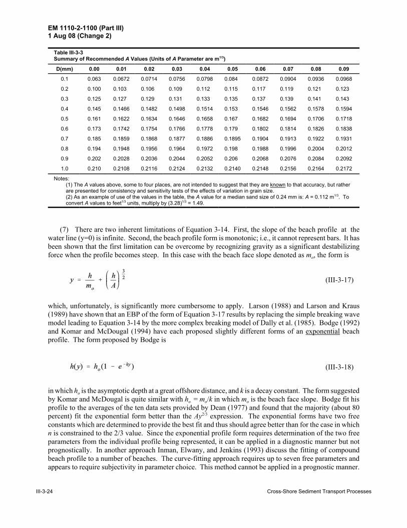
(4) Moore (1982) and Dean (1987b) have provided empirical correlations between the sediment scaleparameter A as a function of sediment size D and fall velocity wf as shown in Figure III-3-17. These resultsare based on a least-squares fit of Equation 3-14 to measured beach profiles. Figure III-3-18 presents anexpanded version of the A versus D relationship for grain sizes more typical of beach sands and Table III-3-3provides a tabulation of A values over the size range D = 0.10 mm to D = 1.09 mm. Although Table III-3-3provides A values to four decimal places at diameter increments of 0.01 mm, this should not be interpretedas signifying that understanding of EBP justifies this level of quantification. Rather the values are presentedfor consistency by different users and possibly for use in sensitivity tests.
(5) The equilibrium profile parameter A may also be correlated to sediment fall velocity. In Fig-ure III-3-17, a relationship is suggested between A and wf that is valid over the entire range of sediment sizesshown. Kriebel, Kraus, and Larson (1991) developed a similar correlation over a range of typical sand grainsizes from D = 0.1 mm to D = 0.4 mm and found the following relationship
(6) This dependence of A on fall velocity to the two-thirds power has also been suggested by Hughes(1994) based on dimensional analysis.

EM 1110-2-1100 (Part III)1 Aug 08 (Change 2)
Cross-Shore Sediment Transport Processes III-3-23
Figure III-3-17. Variation of sediment scale parameter A with sediment size D and fall velocity wf (Dean1987b)
0.06
0.08
0.1
0.12
0.14
0.16
0.18
0.2
0.22
Sca
le P
aram
eter
A
0 0.2 0.4 0.6 0.8 1 1.2 Median Sed Size D (mm)
Figure III-3-18. Variation of sediment scale parameter A(D) with sediment size D for beach sandsizes (based on Dean 1978b, values recomputed by Dean, June 2001)
EM 1110-2-1100 (Part III)1 Aug 08 (Change 2)
III-3-24 Cross-Shore Sediment Transport Processes
(III-3-17)
(III-3-18)
Table III-3-3Summary of Recommended A Values (Units of A Parameter are m1/3)
D(mm) 0.00 0.01 0.02 0.03 0.04 0.05 0.06 0.07 0.08 0.09
0.1 0.063 0.0672 0.0714 0.0756 0.0798 0.084 0.0872 0.0904 0.0936 0.0968
0.2 0.100 0.103 0.106 0.109 0.112 0.115 0.117 0.119 0.121 0.123
0.3 0.125 0.127 0.129 0.131 0.133 0.135 0.137 0.139 0.141 0.143
0.4 0.145 0.1466 0.1482 0.1498 0.1514 0.153 0.1546 0.1562 0.1578 0.1594
0.5 0.161 0.1622 0.1634 0.1646 0.1658 0.167 0.1682 0.1694 0.1706 0.1718
0.6 0.173 0.1742 0.1754 0.1766 0.1778 0.179 0.1802 0.1814 0.1826 0.1838
0.7 0.185 0.1859 0.1868 0.1877 0.1886 0.1895 0.1904 0.1913 0.1922 0.1931
0.8 0.194 0.1948 0.1956 0.1964 0.1972 0.198 0.1988 0.1996 0.2004 0.2012
0.9 0.202 0.2028 0.2036 0.2044 0.2052 0.206 0.2068 0.2076 0.2084 0.2092
1.0 0.210 0.2108 0.2116 0.2124 0.2132 0.2140 0.2148 0.2156 0.2164 0.2172
Notes:(1) The A values above, some to four places, are not intended to suggest that they are known to that accuracy, but ratherare presented for consistency and sensitivity tests of the effects of variation in grain size.(2) As an example of use of the values in the table, the A value for a median sand size of 0.24 mm is: A = 0.112 m1/3. Toconvert A values to feet1/3 units, multiply by (3.28)1/3 = 1.49.
(7) There are two inherent limitations of Equation 3-14. First, the slope of the beach profile at thewater line (y=0) is infinite. Second, the beach profile form is monotonic; i.e., it cannot represent bars. It hasbeen shown that the first limitation can be overcome by recognizing gravity as a significant destabilizingforce when the profile becomes steep. In this case with the beach face slope denoted as mo, the form is
which, unfortunately, is significantly more cumbersome to apply. Larson (1988) and Larson and Kraus(1989) have shown that an EBP of the form of Equation 3-17 results by replacing the simple breaking wavemodel leading to Equation 3-14 by the more complex breaking model of Dally et al. (1985). Bodge (1992)and Komar and McDougal (1994) have each proposed slightly different forms of an exponential beachprofile. The form proposed by Bodge is
in which ho is the asymptotic depth at a great offshore distance, and k is a decay constant. The form suggestedby Komar and McDougal is quite similar with ho = mo/k in which mo is the beach face slope. Bodge fit hisprofile to the averages of the ten data sets provided by Dean (1977) and found that the majority (about 80percent) fit the exponential form better than the Ay2/3 expression. The exponential forms have two freeconstants which are determined to provide the best fit and thus should agree better than for the case in whichn is constrained to the 2/3 value. Since the exponential profile form requires determination of the two freeparameters from the individual profile being represented, it can be applied in a diagnostic manner but notprognostically. In another approach Inman, Elwany, and Jenkins (1993) discuss the fitting of compoundbeach profile to a number of beaches. The curve-fitting approach requires up to seven free parameters andappears to require subjectivity in parameter choice. This method cannot be applied in a prognostic manner.

EM 1110-2-1100 (Part III)1 Aug 08 (Change 2)
Cross-Shore Sediment Transport Processes III-3-25
d. Computation of equilibrium beach profiles. The most simple application is the calculation ofequilibrium beach profiles for various grain sizes, assumed uniform across the profile. This application isillustrated by the following example.
The extension of the equilibrium profile form to cases where the grain size varies across the profile isdiscussed in Dean (1991).
e. Application of equilibrium profile methods to nourished beaches.
(1) In the design of beach nourishment projects, it is important to estimate the dry beach width afterprofile equilibration. Most profiles are placed at slopes considerably steeper than equilibrium and theequilibration process, consisting of a redistribution of the fill sand across the active profile out to the depthof closure, occurs over a period of several years. In general, the performance of a beach fill, in terms of theresulting gain in dry beach width relative to the volume of sand placed on the beach, is a function of thecompatibility of the fill sand with the native sand. Based on equilibrium beach profile concepts, it should beevident that since profiles composed of coarser sediments assume steeper profiles, beach fills using coarsersand will require less sediment to provide the same equilibrium dry beach width )y than fills using sedimentthat is finer than the native sand.
(2) It can be shown that three types of nourished profiles are possible, depending on the volumes addedand on whether the nourishment is coarser or finer than that originally present on the beach. These profilesare termed “intersecting,” “nonintersecting,” and “submerged,” respectively, and are shown in Figure III-3-20. It can be shown that an intersecting profile requires the added sand to be coarser than the native sand,although this condition does not guarantee intersecting profiles, since the intersection may be at a depth inexcess of the depth of closure. Nonintersecting or submerged profiles always occur if the sediment is of thesame diameter or finer than the native sand.
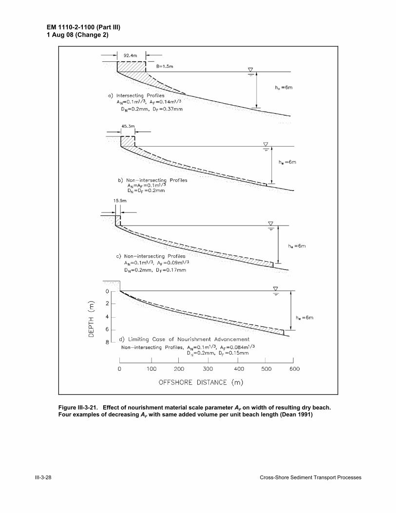
(3) Several more general examples will assist in understanding the significance of the sand and volumecharacteristics. Denoting the sediment scale parameters for the native and fill sediments as AN and AF,respectively, Figure III-3-21 presents the variation in dry beach width for a native sand size of 0.20 mm andvarious fill diameters ranging from 0.15 mm to 0.40 mm. These results are illustrated for a closure depth h*of 6 m, a berm height B of 2 m, and a volumetric addition per unit beach length of 340 m3/m. In the upperpanel, the fill sediment is coarser than the native sand and the profiles are intersecting, resulting in anequilibrium additional dry beach width of 92.4 m. In the second panel, the fill sand is of the same size as thenative (nonintersecting profiles) and the added beach width is 45.3 m. The third and fourth panels illustratethe effects of further decreases in sediment sizes with an incipient submerged profile in the last panel. Theseexamples have considered the effects only of cross-shore equilibration. In design of beach nourishmentprojects, the additional effects of more rapid spreading out of the nourishment project due to longshoresediment transport due to fine sediments should also be considered. The next generic example, presented inFigure III-3-22, illustrates the effects of adding greater amounts of sediment that are finer than the native.For small amounts, the profile is totally submerged. However, as greater and greater amounts are added, thelandward extremity of the nourished profile advances toward land, and ultimately the profile becomesemergent.

EM 1110-2-1100 (Part III)1 Aug 08 (Change 2)
III-3-26 Cross-Shore Sediment Transport Processes
-7
-6
-5
-4
-3
-2
-1
0
Dep
th h
(m)
0 50 100 150 200 Distance offshore y (m)
D = 0.3 mm
D = 0.66 mm
Figure III-3-19. Equilibrium beach profiles for sand sizes of 0.3 mm and 0.66 mmA(D = 0.3 mm) = 0.125 m1/3, A(D = 0.66 mm) = 0.18 m1/3
(III-3-19)
EXAMPLE PROBLEM III-3-1FIND:
The equilibrium beach profiles.
GIVEN:Consider grain sizes of 0.3 mm and 0.66 mm.
SOLUTION:From Figure III-3-18 and/or Table III-3-3, the associated A values are 0.125 m1/3 and 0.18 m1/3,
respectively. Applying Equation 3-14, the two profiles are computed and are presented in Fig-ure III-3-19. The profile composed of the coarser sand is considerably steeper than that for the finermaterial.
f. Quantitative relationships for nourished profiles.
(1) In order to investigate the conditions of profile type occurrence and additional quantitative aspects,it is useful to define the following nondimensional quantities: AN= AF/AN, )yN = )y/W*, BN= B/h*, and VN=V/(B W*), where the symbol V denotes added volume per unit beach length, B is the berm height, and h* isthe depth to which the nourished profile will equilibrate as shown in Figure III-3-21. In general, this will beconsidered to be the closure depth. It is important to note that the width W* is based on the native sedimentscale parameter AN as given by
EM 1110-2-1100 (Part III)1 Aug 08 (Change 2)
Cross-Shore Sediment Transport Processes III-3-27
Figure III-3-20. Three generic types of nourished profiles. (a) intersecting, (b)nonintersecting, and (c) submerged profiles (Dean 1991)
EM 1110-2-1100 (Part III)1 Aug 08 (Change 2)
III-3-28 Cross-Shore Sediment Transport Processes
Figure III-3-21. Effect of nourishment material scale parameter AF on width of resulting dry beach. Four examples of decreasing AF with same added volume per unit beach length (Dean 1991)

EM 1110-2-1100 (Part III)1 Aug 08 (Change 2)
Cross-Shore Sediment Transport Processes III-3-29
Figure III-3-22. Effect of increasing volume of sand added on resulting beachprofile. AF = 0.1 m1/3, AN = 0.2 m1/3, h* = 6.0 m, B = 1.5 m (Dean 1991)

EM 1110-2-1100 (Part III)1 Aug 08 (Change 2)
III-3-30 Cross-Shore Sediment Transport Processes
(III-3-20)
(III-3-21)
(III-3-22)
(III-3-23)
(III-3-24)
(III-3-25)
It is possible to show that the nondimensional equilibrium dry beach width )yN can be presented in terms ofthree nondimensional quantities
(2) The relationships governing the conditions for intersecting/nonintersecting profiles are
given that the fill sediment scale parameter is greater than or equal to the native sediment scale parameter.
The critical volume of sand delineating intersecting and nonintersecting profiles is
which applies only for AN>1, since for AN<1, the profiles will always be nonintersecting although it shouldbe recognized that nonintersecting profiles can also exist for AN>1. If AN>1, but VN > Vc1, then the profilewill be nonintersecting. Also of interest is the critical volume of sand Vc2 that will just yield a finite shorelinedisplacement for the case of sand that is finer than the native (AN<1)
(3) Figure III-3-23 presents these two critical volumes versus the scale parameter AN for the special caseBN=0.25.
(4) For intersecting profiles, the nondimensional volume required to yield an advancement )yN is
This equation would apply for the example in Figure III-3-20a.
(5) For nonintersecting but emergent profiles, the corresponding volume V2N is
This equation would apply for Figure III-3-20b.

EM 1110-2-1100 (Part III)1 Aug 08 (Change 2)
Cross-Shore Sediment Transport Processes III-3-31
0
5
10
15
V'
0
1
2
3
V'
0 1 2 3 A'
Eq. III-3-22
Eq. III-3-23
Region of non-intersectingprofiles
Region ofintersecting profiles
Figure III-3-23. (1) Volumetric requirement for finite shoreline advancement (Equa-tion 3-23); (2) Volumetric requirement for intersecting profiles (Equation 3-22). Results presented for special case BN = 0.25
(III-3-26)
(III-3-27)
(6) For submerged profiles, referring to Figure III-3-20c, it can be shown that
where )yN<0, AN < 1, and the nondimensional volume of sediment can be expressed as
where
This equation would apply for Figure III-3-20c but is of limited value since no beach width would be added.
EM 1110-2-1100 (Part III)1 Aug 08 (Change 2)
III-3-32 Cross-Shore Sediment Transport Processes
(III-3-28)
(7) Equations 3-24 and 3-25 can be displayed in a useful form for calculating the volume required fora particular equilibrium additional dry beach width. However, as is evident from Equation 3-20, there arethree independent variables: BN, AN, and VN. Thus, since only two independent variables can be displayedon a single plot, it is necessary to have a series of plots. Three are presented here, one each for BN = 0.5 (Fig-ure III-3-24) BN = 0.333 (Figure III-325) and BN = 0.25 (Figure III-3-26). The information contained in theseplots will be discussed by reference to Figure III-3-24.
(8) The vertical axis is the nondimensional added beach width )yN, the horizontal axis is thenondimensional sediment scale parameter AN, and the isolines are the nondimensional volumes VN. For agiven AN and VN, the value of )yN is readily determined. It is seen that )yN increases with increasing VN andAN. The heavy dashed line delineates the regions of intersecting and nonintersecting profiles (Equation 3-23).With decreasing AN and constant VN, the value of )yN decreases to the asymptotes for a submerged profile.Several examples will be presented illustrating the application of Figures III-3-24, III-3-25, and III-3-26.
g. Longshore bar formation and seasonal shoreline changes.
(1) Longshore bars were discussed briefly in Part III-3-2. They are elongated mounds more or lessparallel to the shoreline and are known to be more prevalent for storm conditions and for finer sediments.Bars may be present as single features or may occur as a series (Figure III-3-10). Additionally, bars can beseasonal or perennial. In most locations where bars are seasonal, their formation is associated with a seawardtransport of sediment and a retreat of the shoreline. At a particular location, the amount of seasonalfluctuation depends on the number and intensity of storms during a particular year. Figure III-3-30 showsresults of measurements by Dewall and Richter (1977) from Jupiter Island, Florida, where the seasonalfluctuations appear to be on the order of 15 m. Figure III-3-31, from Dewall (1979) shows shoreline andvolume changes (above mean sea level) from Westhampton, Long Island, New York, where the seasonalchanges may be on the order of 20 to 40 m.
(2) Although the prediction of bar geometry and the associated shoreline changes have not advancedto a reliable stage, parameters have been proposed and correlated successfully with conditions for which barsform. Based on field observations, Dean (1973) hypothesized that sediment was suspended during the crestphase position and that if the fall time were less or greater than one-half the wave period, the net transportwould be landward or seaward, respectively, resulting in bar formation in the latter case. This mechanismwould be consistent with the wave-breaking cause. Further rationalizing that the suspension height wouldbe proportional to the wave height resulted in identification of the so-called fall velocity parameter Hb/wfT.Although there is no agreement on the cause of longshore bar formation, it appears to result from wavebreaking, with edge waves and other phenomena proposed as possible causes.
(3) Examination of small-scale laboratory data for which the deep water reference wave height Hovalues were available led to the following relationship (Dean 1973) for offshore sediment transport leadingto bar formation
(4) Later, Kriebel, Dally, and Dean (1986) examined only prototype and large-scale laboratory data andfound a constant of approximately 2.8 rather than 0.85 as in Equation 3-28. Kraus, Larson, and Kriebel(1991) examined only large wave tank data and proposed the following two relationships for barformation

EM 1110-2-1100 (Part III)1 Aug 08 (Change 2)
Cross-Shore Sediment Transport Processes III-3-33
0.0001
0.001
0.01
0.1
1
)(r
0 1 2 3 A'
V' = 0.001
V' = 0.002
V' = 0.005
V' = 0.01
V' = 0.02
V' = 0.05
V' = 0.1
V' = 0.2
V' = 0.5
V' = 1.0V' =2.0
V' = 5.0V' = 10.0
B' = 0.5
Non-intersecting
Profiles
IntersectingProfiles
Critical Line
Figure III-3-24. Variation of nondimensional shoreline advancement )y/W*, with AN and V. Resultsshown for H*/B = 2.0 (BN = 0.5) (based on Dean (1991), values recomputed by Dean, May 2001). Intersecting and non-intersecting profiles divided by critical line; definition sketches shown inFigure III-3-20.
(III-3-29)
(III-3-30)
and

EM 1110-2-1100 (Part III)1 Aug 08 (Change 2)
III-3-34 Cross-Shore Sediment Transport Processes
0.0001
0.001
0.01
0.1
1
)(r
0 1 2 3 A'
V' = 0.001
V' = 0.002
V' = 0.005
V' = 0.01
V' = 0.02
V' = 0.05
V' = 0.1
V' = 0.2
V' = 0.5
V' = 1.0
V' =2.0V' = 5.0V' = 10.0
B' = 0.333
Non-intersecting
Profiles
IntersectingProfiles
Critical Line
Figure III-3-25. Variation of nondimensional shoreline advancement )y/W*, with AN and V. Resultsshown for H*/B = 3.0 (BN = 0.333) (based on Dean (1991), values recomputed by Dean, May 2001). Intersecting and non-intersecting profiles divided by critical line; definition sketches shown inFigure III-3-20.
(III-3-31)
in which Ho is the average deepwater wave height. For field data in which the significant deepwater waveheight was used, the constant in Equation 3-30 was modified to
(5) It is interesting that Equation 3-30 provides a better fit to the laboratory data than a fixed value ofthe fall velocity parameter; however, for field data, a fixed value of the fall velocity parameter provides a

EM 1110-2-1100 (Part III)1 Aug 08 (Change 2)
Cross-Shore Sediment Transport Processes III-3-35
0.0001
0.001
0.01
0.1
1
)(r
0 1 2 3 A'
V' = 0.001
V' = 0.002
V' = 0.005
V' = 0.01
V' = 0.02
V' = 0.05
V' = 0.1
V' = 0.2
V' = 0.5
V' = 1.0
V' =2.0V' = 5.0V' = 10.0
B' = 0.25
Non-intersecting
ProfilesIntersecting
Profiles
Critical Line
Figure III-3-26. Variation of nondimensional shoreline advancement )y/W*, with AN and V. Resultsshown for H*/B = 4.0 (BN = 0.25), based on Dean (1991), values recomputed by Dean, May 2001). Intersecting and non-intersecting profiles divided by critical line; definition sketches shown inFigure III-3-20.
(III-3-32)
better fit than Equation 3-30 (Kraus, Larson, and Kriebel 1991). Dalrymple (1992) has shown thatEquations 3-29 and 3-30 can be represented in terms of a single profile parameter P where
and that the criterion for bar formation is that P exceeds about 10,000.

EM 1110-2-1100 (Part III)1 Aug 08 (Change 2)
III-3-36 Cross-Shore Sediment Transport Processes
EXAMPLE PROBLEM III-3-2FIND:
The equilibrated additional dry beach width )y due to cross-shore transport.
GIVEN:DN = 0.2 mm, DF = 0.24 mm, B = 2 m, V = 400 m3/m.
H6 = 1.5 m, FH = 0.64 m as provided in WES and CEDRS databases discussed in Part II-8.
SOLUTION:Based on the above, the sediment scale parameters are determined from Figure III-3-18 and/or
Table III-3-3 to be: AN = 0.1 m1/3, AF = 0.11 m1/3. The effective wave height He is determined fromEquation 3-10 as:
He = H6 + 5.6 FH = 1.5 + (5.6)(0.64) – 5.1 m
The closure depth h* is determined from Equation 3-12 as:
h* = hC = 1.57 He = (1.57) (5.11) – 8 m
The reference width of effective motion W* is based on Equation 3-19
With this information, it is possible to determine the following nondimensional quantities:
BN = B/h* = 2/8 = 0.25, AN = AF/AN = 0.11/0.1 = 1.1
VN = V/(BW*) = 400/(2)(716) – 0.28
Since BN = 0.25, Figure III-3-26 is applicable and for AN = 1.1 and VN = 0.28, it is found that )yN = 0.092.Thus )y = (0.092)(716) – 65.9 m. Also, it is seen from Figure III-3-26 that this solution is near theboundary of the intersecting/nonintersecting profiles.The native and nourished profiles are shown inFigure III-3-27. The solution is next carried out with the appropriate equations for comparison with thegraphical procedure. Applying Equation 3-22 to determine whether the profiles will be intersecting ornonintersecting
compared with the applied VN of 0.28. Thus since VN<(VN)c1 the solution is an intersecting profile.Applying Equation 3-24 requires an iterative solution for )yN. This equation can be reduced to
0.28 = )yN + 9.20()yN)5/3
the solution to which yields )yN = 0.0955 or )y = 68.4 m(Continued)

EM 1110-2-1100 (Part III)1 Aug 08 (Change 2)
Cross-Shore Sediment Transport Processes III-3-37
Figure III-3-27. Nourishment with coarser sand than native (intersecting profiles)
Example Problem III-3-2 (Concluded)Thus, for this example, the graphical solution is reasonable. The calculated intersection distance forthe two profiles yI is determined from
or
and
By comparison, the corresponding values from the graphical solution are yI = 495 m and hI = 6.25 m.Figure III-3-27 presents the results of the graphical solution.

EM 1110-2-1100 (Part III)1 Aug 08 (Change 2)
III-3-38 Cross-Shore Sediment Transport Processes
EXAMPLE PROBLEM III-3-3FIND:
V, the volume of sand necessary to achieve the additional dry beach width )y of 50 m.
GIVEN:B=2 m, DN = DF = 0.25 mm, )y = 50 m, where H6=1.5 m, FH = 0.4 m.
SOLUTION:
The value of h* is computed as:
h* = 1.57 (H6 + 5.6 FH) = 1.57 [1.5 + (5.6)(0.4)] – 5.9 m
For these values, the associated A values are determined from Figure III-3-18 and/or Table III-3-3 to be:AN = AF = 0.115 m1/3. The reference width of active motion W* is
and the required nondimensional quantities are:
)y/W* – 50/367 – 0.136, BN = B/h* – 0.34, AN = AF/AN = 0.115/0.115 = 1.0
Since the value of BN lies between the two values represented in Figures III-3-24 and III-3-26, it isnecessary to interpolate. The values from these two figures are: VN(BN = 0.25) = 0.75, VN(BN = 0.5) =0.35. Interpolating linearly, VN is found to be 0.606 for the desired BN value of 0.34, from which thevolume V is determined as V = VN B W* = (0.606) (2) (367) – 445 m3/m. Since the fill and nativesediments are of the same size, it is clear that the two profiles will be nonintersecting and thatEquation 3-25 can be used to compute the nondimensional volume directly
(Continued)
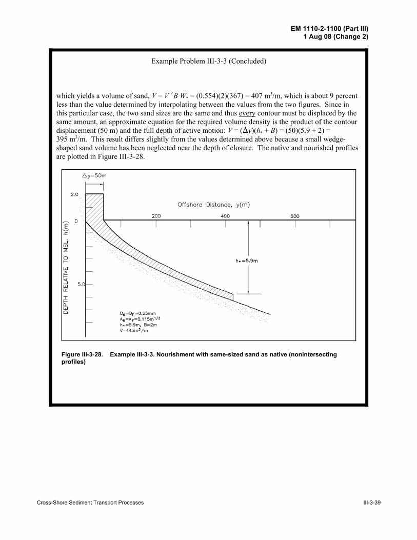
EM 1110-2-1100 (Part III)1 Aug 08 (Change 2)
Cross-Shore Sediment Transport Processes III-3-39
Figure III-3-28. Example III-3-3. Nourishment with same-sized sand as native (nonintersectingprofiles)
Example Problem III-3-3 (Concluded)
which yields a volume of sand, V = VN B W* = (0.554)(2)(367) = 407 m3/m, which is about 9 percentless than the value determined by interpolating between the values from the two figures. Since inthis particular case, the two sand sizes are the same and thus every contour must be displaced by thesame amount, an approximate equation for the required volume density is the product of the contourdisplacement (50 m) and the full depth of active motion: V = ()y)(h* + B) = (50)(5.9 + 2) =395 m3/m. This result differs slightly from the values determined above because a small wedge-shaped sand volume has been neglected near the depth of closure. The native and nourished profilesare plotted in Figure III-3-28.
EM 1110-2-1100 (Part III)1 Aug 08 (Change 2)
III-3-40 Cross-Shore Sediment Transport Processes
Figure III-2-29. Illustration of effect of volume added V and fill sediment scaleparameter AF on additional dry beach width )y. Example conditions: B = 1.5 m,h* = 6 m, AN = 0.1 m1/3
EXAMPLE PROBLEM III-3-4FIND:
The variation in equilibrated dry beach width with volume added for three candidate fill sand sizes.
GIVEN:Three candidate borrow sites with representative sand sizes: = 0.15 mm, = 0.2 mm and
= 0.25 mm. The native sand size, DN = 0.2 mm. The berm height B = 1.5 m and h* = 6 m.
SOLUTION:The associated values of the sediment scale parameters are determined from Figure III-3-18 and/or
Table III-3-3: AN = 0.1 m1/3, = 0.084 m1/3, = 0.1 m1/3, and = 0.115 m1/3, respectively.
The procedures illustrated in Example Problems III-3-2 and III-3-3 produce the results shown inFigure III-3-29. It is seen that there is a nearly linear relationship for the sand that is of the same sizeas the native in accordance with: V =()y)(h* + B). For the fill sand, which is coarser than the native, forvolumes less than approximately 450 m3/m, the increase in dry beach width for each volume added isgreater than for the same-sized sand. For this region, the profiles are intersecting. For greater volumes,the profiles are nonintersecting and the slope of the relationship is nearly the same as for AF/AN = 1.0.For the sand smaller than the native, the profiles are submerged for the smaller volumes and later becomeemergent in accordance with Equation 3-23. For larger volumes, the relationship has approximately thesame slope as that for sand the same size as the native. The explanation for this is that once the profilesbecome emergent and nonintersecting, additional volumes of sand added simply displace the profile withall contours moving the same distance over the active depth. Thus the slope in Figure III-3-29 for thissituation is nearly independent of the grain size.

EM 1110-2-1100 (Part III)1 Aug 08 (Change 2)
Cross-Shore Sediment Transport Processes III-3-41
Figure III-3-30. Mean monthly shoreline position (A) and unit volume (B) at Jupiter Island, FL, referenced tofirst survey (Dewall and Richter 1977)
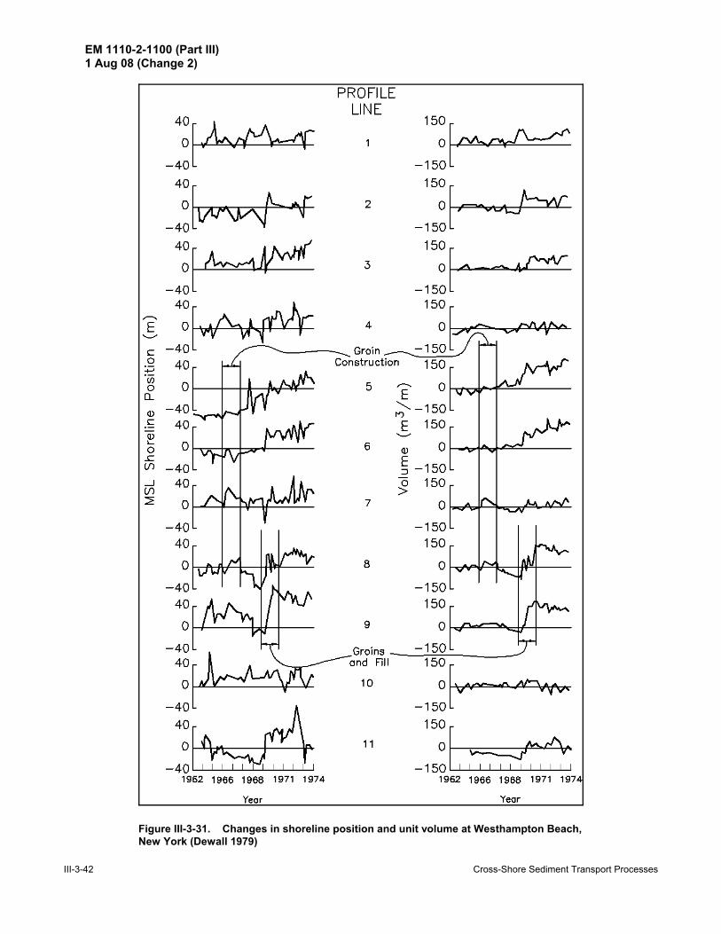
EM 1110-2-1100 (Part III)1 Aug 08 (Change 2)
III-3-42 Cross-Shore Sediment Transport Processes
Figure III-3-31. Changes in shoreline position and unit volume at Westhampton Beach,New York (Dewall 1979)
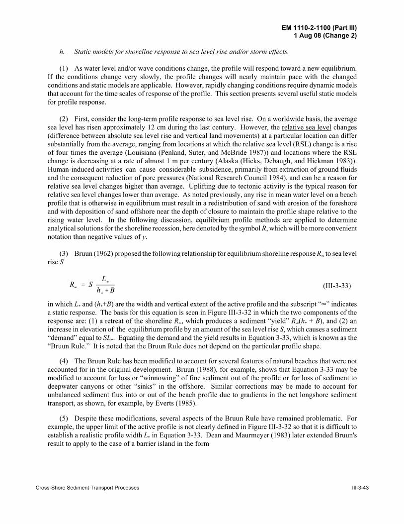
EM 1110-2-1100 (Part III)1 Aug 08 (Change 2)
Cross-Shore Sediment Transport Processes III-3-43
(III-3-33)
h. Static models for shoreline response to sea level rise and/or storm effects.
(1) As water level and/or wave conditions change, the profile will respond toward a new equilibrium.If the conditions change very slowly, the profile changes will nearly maintain pace with the changedconditions and static models are applicable. However, rapidly changing conditions require dynamic modelsthat account for the time scales of response of the profile. This section presents several useful static modelsfor profile response.
(2) First, consider the long-term profile response to sea level rise. On a worldwide basis, the averagesea level has risen approximately 12 cm during the last century. However, the relative sea level changes(difference between absolute sea level rise and vertical land movements) at a particular location can differsubstantially from the average, ranging from locations at which the relative sea level (RSL) change is a riseof four times the average (Louisiana (Penland, Suter, and McBride 1987)) and locations where the RSLchange is decreasing at a rate of almost 1 m per century (Alaska (Hicks, Debaugh, and Hickman 1983)).Human-induced activities can cause considerable subsidence, primarily from extraction of ground fluidsand the consequent reduction of pore pressures (National Research Council 1984), and can be a reason forrelative sea level changes higher than average. Uplifting due to tectonic activity is the typical reason forrelative sea level changes lower than average. As noted previously, any rise in mean water level on a beachprofile that is otherwise in equilibrium must result in a redistribution of sand with erosion of the foreshoreand with deposition of sand offshore near the depth of closure to maintain the profile shape relative to therising water level. In the following discussion, equilibrium profile methods are applied to determineanalytical solutions for the shoreline recession, here denoted by the symbol R, which will be more convenientnotation than negative values of y.
(3) Bruun (1962) proposed the following relationship for equilibrium shoreline response R4 to sea levelrise S
in which L* and (h*+B) are the width and vertical extent of the active profile and the subscript “4” indicatesa static response. The basis for this equation is seen in Figure III-3-32 in which the two components of theresponse are: (1) a retreat of the shoreline R4, which produces a sediment “yield” R4(h* + B), and (2) anincrease in elevation of the equilibrium profile by an amount of the sea level rise S, which causes a sediment“demand” equal to SL*. Equating the demand and the yield results in Equation 3-33, which is known as the“Bruun Rule.” It is noted that the Bruun Rule does not depend on the particular profile shape.
(4) The Bruun Rule has been modified to account for several features of natural beaches that were notaccounted for in the original development. Bruun (1988), for example, shows that Equation 3-33 may bemodified to account for loss or “winnowing” of fine sediment out of the profile or for loss of sediment todeepwater canyons or other “sinks” in the offshore. Similar corrections may be made to account forunbalanced sediment flux into or out of the beach profile due to gradients in the net longshore sedimenttransport, as shown, for example, by Everts (1985).
(5) Despite these modifications, several aspects of the Bruun Rule have remained problematic. Forexample, the upper limit of the active profile is not clearly defined in Figure III-3-32 so that it is difficult toestablish a realistic profile width L* in Equation 3-33. Dean and Maurmeyer (1983) later extended Bruun'sresult to apply to the case of a barrier island in the form

EM 1110-2-1100 (Part III)1 Aug 08 (Change 2)
III-3-44 Cross-Shore Sediment Transport Processes
Figure III-3-32. Components of sand volume balance due to sea level rise and associated profileretreat according to the Bruun Rule

EM 1110-2-1100 (Part III)1 Aug 08 (Change 2)
Cross-Shore Sediment Transport Processes III-3-45
(III-3-34)
Figure III-3-33. The Bruun Rule generalized for the case of a barrier island that maintains its form relative tothe adjacent ocean and lagoon (Dean and Maurmeyer 1983)
(III-3-35)
and the various terms are explained in Figure III-3-33. In general, the shoreline retreat is some 50 to200 times the sea level rise with the greater factors associated with the milder beach slopes and moreenergetic wave conditions (i.e., greater h*). These factors for the case of a barrier island would beconsiderably greater due to the difference term in the denominator (Equation 3-34). Situations where theregion behind the island is deep may explain the geological evidence for some barrier islands which arebelieved to have “drowned in place” rather than to have migrated landward.
(6) The Bruun Rule has been subjected to verifications both in the laboratory and in the field. Hands(1983), evaluated the Bruun Rule in Lake Michigan using 25 beach profiles over a 50-km length of shorelinesubjected to a 0.2-m water level rise over a 7-year period from 1969 to 1976. The on- and offshore limits ofprofile response were determined directly from measured beach profiles. Thus, the depth of closure wasidentified as the maximum depth of significant profile change observed from beach surveys. Likewise, theupper limit of profile change was selected as the natural vegetation line in the foredunes. With theseempirical input parameters, calculated profile retreat over the 7-year period then agreed to within 10 percentof measured values. Over shorter periods of time for example, over a 3-year period, Hands found that theBruun Rule initially over-estimated the profile response due to the time lag between elevated water levels andthe profile response. Storm processes were then identified as being responsible for causing rapid equilibrationof the profiles and for causing the profiles to “catch up” or equilibrate relative to the water level.
(7) Edelman (1972) modified the Bruun Rule to make it more appropriate for larger values of increasedwater levels and for time-varying storm surges. It was assumed that the profile maintained pace with therising sea level and thus, at each time, the following equation is valid
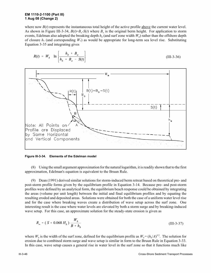
EM 1110-2-1100 (Part III)1 Aug 08 (Change 2)
III-3-46 Cross-Shore Sediment Transport Processes
(III-3-36)
Figure III-3-34. Elements of the Edelman model
(III-3-37)
where now B(t) represents the instantaneous total height of the active profile above the current water level.As shown in Figure III-3-34, B(t)=Bo-S(t) where Bo is the original berm height. For application to stormevents, Edelman also adopted the breaking depth hb (and surf zone width Wb) rather than the offshore depthof closure h* (and corresponding W*) as would be appropriate for long-term sea level rise. SubstitutingEquation 3-35 and integrating gives
(8) Using the small argument approximation for the natural logarithm, it is readily shown that to the firstapproximation, Edelman's equation is equivalent to the Bruun Rule.
(9) Dean (1991) derived similar solutions for storm-induced berm retreat based on theoretical pre- andpost-storm profile forms given by the equilibrium profile in Equation 3-14. Because pre- and post-stormprofiles were defined by an analytical form, the equilibrium beach response could be obtained by integratingthe areas (volume per unit length) between the initial and final equilibrium profiles and by equating theresulting eroded and deposited areas. Solutions were obtained for both the case of a uniform water level riseand for the case where breaking waves create a distribution of wave setup across the surf zone. Oneinteresting result is the case where water levels are elevated by both a storm surge and by breaking-inducedwave setup. For this case, an approximate solution for the steady-state erosion is given as
where Wb is the width of the surf zone, defined for the equilibrium profile as Wb = (hb/A)3/2. The solution forerosion due to combined storm surge and wave setup is similar in form to the Bruun Rule in Equation 3-33.In this case, wave setup causes a general rise in water level in the surf zone so that it functions much like
EM 1110-2-1100 (Part III)1 Aug 08 (Change 2)
Cross-Shore Sediment Transport Processes III-3-47
(III-3-38)
(III-3-39)
(III-3-40)
storm surge. It is noted, however, that storm surge has a much larger effect than wave setup. For this reason,the other analytical solutions that follow do not include wave setup effects and, instead, assume that beachresponse is driven primarily by storm surge.
(10) Kriebel and Dean (1993) considered both profiles with a vertical face at the water line as shown inFigure III-3-35a and profiles with a sloping beach face as shown in Figure III-3-35b. They showed that byaccounting for the small wedge-shaped sand volume offshore of the breaking depth, somewhat improvedexpressions could be developed for the potential beach recession due to elevated water levels. The beachprofile with a vertical face is a special limiting case of the profile with a sloping beach face, thus only theresults for the sloping beach face are given here. As shown by Kriebel and Dean (1993), the general resultfor equilibrium berm recession due to a storm surge level S is given as
where mo is the slope of the beach profile at the waterline. This slope is joined to the concave equilibriumprofile at a depth where the slope of the equilibrium profile is equal to mo. As a result, the surf zone widthcan be shown to be equal to
where yo is a small offset of the shoreline between the sloping beach face and the imaginary or virtual originof the equilibrium profile, given by yo = (4A3)/(27mo
3). For most conditions, this offset is negligible and canbe neglected when estimating the surf zone width, as will be illustrated in Example Problem III-3-6. Forengineering application, it is also of interest to compute the volume of sand eroded between the initial andfinal profiles per unit length of beach. For the case with a sloping beach face, the volume eroded from theberm above the initial still-water level due to a storm surge level S is given by
(11) When the beach face slope becomes infinite, the solutions from Equation 3-38 for the vertical beachface depicted in Figure III-3-35a are similar to those obtained by the Bruun Rule in Equation 3-33 or by Dean(1991) in Equation 3-37. The major difference is the term S/2 in the denominator of Equation 3-38, whichis the result of considering the small wedge-shaped volume of sand near the breakpoint. For more realisticbeach face slopes, the results in Equation 3-38 will yield smaller estimates of the potential berm recessionthan the Bruun or Dean solutions, since a portion of the rise in water level is accommodated by shifting theshoreline higher on the sloping beach face and less berm retreat is then required. Kriebel and Dean (1993)also provide analytical solutions for cases where the beach profile has a distinct dune on top of the berm.
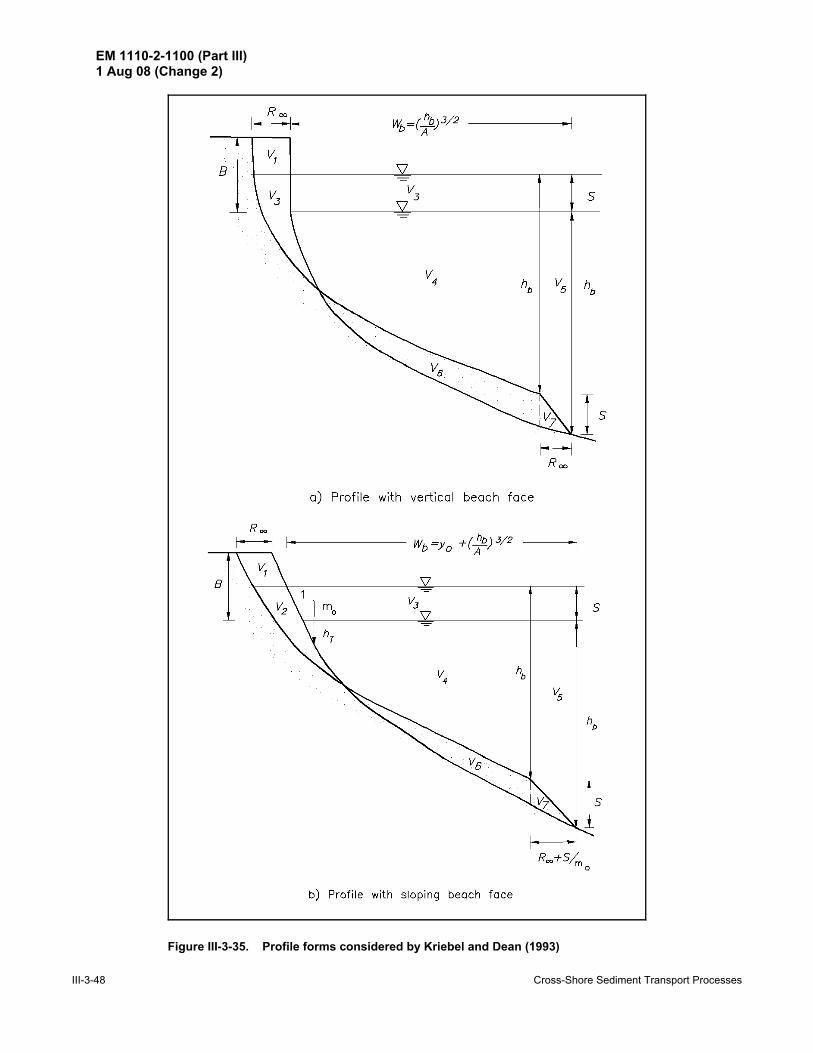
EM 1110-2-1100 (Part III)1 Aug 08 (Change 2)
III-3-48 Cross-Shore Sediment Transport Processes
Figure III-3-35. Profile forms considered by Kriebel and Dean (1993)

EM 1110-2-1100 (Part III)1 Aug 08 (Change 2)
Cross-Shore Sediment Transport Processes III-3-49
EXAMPLE PROBLEM III-3-5
FIND:The rate of shoreline retreat, according to the Bruun Rule, then find the rate at which beach
nourishment would be required to maintain the shoreline position.
GIVEN:
h* = 6 m, B = 2 m, D = 0.2 mm, and a rate of sea level rise of .
SOLUTION:
The sediment scale parameter is determined from Figure III-3-18 and/or Table III-3-3 as A =0.1 m1/3. The width W* of the active nearshore zone is determined from Equation 3-19 as
and from Equation 3-33, assuming the berm stays at a constant elevation, the rate of shoreline retreatis given by
so that the ratio of shoreline retreat to sea level rise is about 58.
When considering sea level rise and beach nourishment, from Equation 3-42, the rate at which sandmust be added to offset the erosion due to sea level rise is

EM 1110-2-1100 (Part III)1 Aug 08 (Change 2)
III-3-50 Cross-Shore Sediment Transport Processes
EXAMPLE PROBLEM III-3-6FIND:
The potential berm retreat, along with the volume of sand eroded from above the mean sea level,for the storm conditions given below.
GIVEN:Equilibrium beach profile with sand grain size D = 0.25 mm, beach face slope mo = 0.05, and
berm height B = 2 m. Storm conditions with a peak surge level S = 2 m and a breaking depth hb =3.0 m.
SOLUTION:The equilibrium berm retreat may be determined from Equation 3-38, which first requires
knowledge of the breaking depth hb and the surf zone width Wb, which, from Equation 3-39, are givenby Wb= yo+(hb/A)3/2. From Table III-3-3, the so-called A parameter for the equilibrium beach profileis found to be A = 0.115 m1/3 based on the grain size of 0.25 mm.
In calculating the surf zone width, the term (hb/A)3/2 is equal to (3.0m/0.115m1/3)3/2 = 133.2 m whilethe small shoreline offset is given by yo = (4A3)/(27mo
3) = 1.8 m. The total surf zone width is then Wb= 1.8 m + 133.2 m = 135.0 m. As noted, however, the offset is negligible and could be neglected forsimplicity.
From Equation 3-38, the potential berm retreat is now determined as
From Equation 3-40, the potential volume eroded from above the mean sea level datum is given by
These solutions are known to generally overestimate erosion associated with severe storms. Forexample, Chiu (1977) compared both the Edelman and Dean methods to erosion measured afterHurricane Eloise on the Florida coast and found that both methods gave erosion estimates that wereas much as a factor of 5 higher than observed. The reason for this overprediction is that thesemethods assume the profile responds instantly to changes in water level while they neglect thetransient or time-dependent approach to equilibrium. Such equilibrium solutions are still useful froman engineering perspective since they place a conservative upper bound on the actual beach response.
(12) While these idealized analytical solutions are useful, such computations of the maximum potentialresponse can also be performed numerically for a measured (surveyed) beach and dune profile. In this case,

EM 1110-2-1100 (Part III)1 Aug 08 (Change 2)
Cross-Shore Sediment Transport Processes III-3-51
(III-3-41)
(III-3-42)
it may be assumed that the existing profile is in a stable equilibrium configuration, possibly with an offshorebar. The solution for the profile response to a water level rise would then be carried out by shifting themeasured profile form upward and landward until a mass balance is achieved between the sand eroded fromthe berm and dune and the sand deposited offshore near the breakpoint.
(13) The problem of shoreline stabilization through beach nourishment with compatible sands in an eraof sea level rise may be treated by combining the two effects. The rate of shoreline retreat is given as
in which dV/dt is the rate at which sand is added per unit length of beach. In order for the shoreline retreatdue to sea level rise to be offset by the advancement due to nourishment, (dR4/dt = 0)
which can be interpreted as adding sufficient sand to just fill the active profile of width W* at the rate of sealevel rise. This result could have been foreseen by referring to Figure III-3-32.
i. Computational models for dynamic response to storm effects.
(1) Introduction. Dynamic computational models are distinguished from the static models discussedearlier by accounting for the transient nature of the profile adjustment. As an illustration, for Example III-3-2,if the initial placement of nourished sand was different (usually steeper) than the equilibrium profile in FigureIII-3-27, it is possible to determine from the equation of continuity (conservation of sand) the total cross-shorevolumetric transport; however, it is not possible to determine the rate at which the sand was transported toreach equilibrium. The equilibration process could have required 1 year or a decade. In many problems ofcoastal engineering interest, the rates are extremely important. As examples, it will be shown that a rapidlymoving storm may cause only a fraction of its erosion potential due to the relatively long time scales of thesediment transport processes and to the relatively short duration of the more energetic conditions caused bythe storm. A second problem in which the time scales are of interest is that of profile equilibration of a beachnourishment project. Although it is accepted that equilibration occurs within 1 to 5 years, and certainlydepends on the frequency of energetic storms, the economic value of that portion of added dry beach widthassociated with disequilibrium during evolution can be substantial.
(2) Numerical and analytical models. More than a dozen numerical models and at least two analyticalmodels have been developed to represent dynamic cross-shore sediment transport processes. These modelsrequire a continuity equation and a transport (or dynamic) equation (or equivalent) that governs the rate atwhich the processes occur. The conservation equation balances the differences between inflows and outflowsfrom a region as predicted by the transport equation. In addition, boundary conditions must be employed atthe landward and seaward ends of the active region. These boundary conditions can usually be expressed interms of a maximum limiting slope such that if the slope is exceeded, adjustment of the profile will occur,a condition sometimes referred to as “avalanching.” The locations of the seaward and landward boundariesare usually taken at the limits of wave breaking and wave runup, respectively. Examples of numerical modelsfor which computer codes are available include those of Kriebel and Dean (1985), Kriebel (1986), Larson(1988), and Larson and Kraus (1989, 1990). Analytical models have been published by Kobayashi (1987),and Kriebel and Dean (1993).
(3) General description of numerical models. In numerical modelling, two representations of thephysical domain have been considered as shown in Figure III-3-36. In the first type, shown in

EM 1110-2-1100 (Part III)1 Aug 08 (Change 2)
III-3-52 Cross-Shore Sediment Transport Processes
(III-3-43)
(III-3-44)
(III-3-45)
(III-3-46)
Figure III-3-36a, the cells are finite increments of the distance variable y. Thus the distance is theindependent variable and the dependent variable is depth, which varies with time. In the second type shownin Figure III-3-36b, the computational cells are formed by finite increments of the depth h. In this case, theindependent variable is h and y varies with time for each h value. There is an inherent advantage of the firsttype since the presence of bars can be represented with no difficulties. All dynamic models require acontinuity equation and a transport (dynamic) equation.
(a) Conservation equation. The conservation equation is very straightforward and for the computationalcell type in Figure III-3-36a is given by
in which y and t are the independent variables. If h and t are regarded as the independent variables as inFigure III-3-36b, the conservation equation is
in which it is noted that for each depth value (h), there is an associated distance value (y).
(b) Transport relationships. Sediment transport relationships fall within the categories of “closed loop,”which converge to a target profile and “open loop,” which are not a priori constrained to the final(equilibrium) profile. Transport relationships of the “closed loop” type will be reviewed first.
(c) Closed loop transport relationships. One of the first closed loop transport relationships was thatproposed by Kriebel and Dean (1985). Recalling that the equilibrium beach profile (EBP) represented byEquation 3-14 is consistent with uniform wave energy dissipation per unit water volume D*, Kriebel and Deanadopted a simple transport relationship in the form
such that at equilibrium D=D*, and an equilibrium profile results. The parameter KN is then used to calibratethe model by correlating the sediment transport rate to the excess energy dissipation. The transportrelationship above may be modified to be consistent with a profile with beach face slope mo
where , is an additional model parameter as suggested by Larson and Kraus (1989). In this expression, thecalibration parameter KNN differs from that used in Equation 3-45, since the additional gravitational effects,represented by the slope term, assist in moving sediment offshore.
(d) Open loop transport relationships. These transport relationships depend on the detailedhydrodynamics and attempt to incorporate the actual processes more faithfully than the closed loop variety.Usually both bed load and suspended load transport components are represented based on the hydrodynamicproperties averaged over a wave period. Open loop models will not be considered further in this chapter;however, an excellent review of open loop models is given by Roelvink and Broker (1993). In general, thesemodels can be grouped according to the physical processes that are assumed to be dominant for cross-shore

EM 1110-2-1100 (Part III)1 Aug 08 (Change 2)
Cross-Shore Sediment Transport Processes III-3-53
Figure III-3-36. Two types of grids employed in numerical modelling of cross-shore sediment transport andprofile evolution
sediment transport. Several models compute transport rates by vertically integrating the distributions ofsuspended sediment concentration and cross-shore currents. Examples of such models include those of Dallyand Dean (1984), Stive and Battjes (1984), and Broker-Hedegaard, Deigaard, and Fredsoe (1991). Othermodels consider instead that bed shear stress is the dominant forcing mechanism. An example is the modelby Watanabe et al. (1980). A third widely used approach has been to compute the combined bed andsuspended load transport first, based on the energetics approach proposed by Bagnold (1966). Examples ofmodels based on this approach include those of Roelvink and Stive (1989) and Nairn and Southgate (1993).

EM 1110-2-1100 (Part III)1 Aug 08 (Change 2)
III-3-54 Cross-Shore Sediment Transport Processes
(III-3-47)
(III-3-48)
(III-3-49)
(4) General description of analytical models.
(a) The analytical model of profile evolution by Kobayashi (1987) incorporates the conservation andtransport relationships (Equations 3-41 and 3-43). The transport equation is linearized such that a diffusionequation results. The landward and seaward receding and advancing limits of the evolving profile are treatedas moving boundary conditions. Kobayashi (1987) presents an analytical solution for the case of a constantelevated water level in the form of fairly complex error functions. For more complete water level scenarios,a numerical scheme must be used. As presented, the model does not lend itself readily to engineeringapplications.
(b) A simpler analytical model for predicting dynamic profile response during storms is the so-calledConvolution Method of Kriebel and Dean (1993). This method is based on the observation that beaches tendto respond toward a new equilibrium exponentially over time. For laboratory conditions, where a beach issuddenly subjected to steady wave action, the time-dependent shoreline response R(t) may be approximatedby the form
where R4 is the equilibrium beach response and TS is the characteristic time-scale of the system. Anexponential response of this kind has been observed in wave tank experiments by Swart (1974), Dette andUliczka (1987), and Larson and Kraus (1989).
(c) A more general result for the dynamic erosion response may be obtained by noting thatEquation 3-47 suggests that the rate of profile response is proportional to the difference between theinstantaneous profile form and the ultimate equilibrium form. An approximate differential equationgoverning the profile response to time-dependent variations in water level may be assumed in the form
where f(t) represents a unit-amplitude function of time that describes the storm surge hydrograph, while R4represents the equilibrium beach response for the peak water level. The general solution to this system maybe expressed as a convolution integral as
(d) As a result, several important characteristics of dynamic beach profile response are evident. First,a beach has a certain “memory,” so that the beach response at any one time is dependent on the forcingconditions applied over some preceding time period. As a result, the beach response will lag behind theerosion forcing. In addition, because of the exponential response characteristics of the beach system, thebeach response will be damped so that the actual maximum response will be less than the erosion potentialof the system.
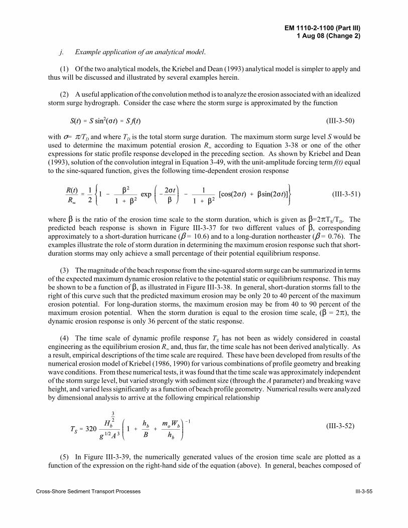
EM 1110-2-1100 (Part III)1 Aug 08 (Change 2)
Cross-Shore Sediment Transport Processes III-3-55
(III-3-50)
(III-3-52)
j. Example application of an analytical model.
(1) Of the two analytical models, the Kriebel and Dean (1993) analytical model is simpler to apply andthus will be discussed and illustrated by several examples herein.
(2) A useful application of the convolution method is to analyze the erosion associated with an idealizedstorm surge hydrograph. Consider the case where the storm surge is approximated by the function
with F= B/TD and where TD is the total storm surge duration. The maximum storm surge level S would beused to determine the maximum potential erosion R4 according to Equation 3-38 or one of the otherexpressions for static profile response developed in the preceding section. As shown by Kriebel and Dean(1993), solution of the convolution integral in Equation 3-49, with the unit-amplitude forcing term f(t) equalto the sine-squared function, gives the following time-dependent erosion response
(III-3-51)
where $ is the ratio of the erosion time scale to the storm duration, which is given as $=2BTS/TD. Thepredicted beach response is shown in Figure III-3-37 for two different values of $, correspondingapproximately to a short-duration hurricane ($ = 10.6) and to a long-duration northeaster ($ = 0.76). Theexamples illustrate the role of storm duration in determining the maximum erosion response such that short-duration storms may only achieve a small percentage of their potential equilibrium response.
(3) The magnitude of the beach response from the sine-squared storm surge can be summarized in termsof the expected maximum dynamic erosion relative to the potential static or equilibrium response. This maybe shown to be a function of $, as illustrated in Figure III-3-38. In general, short-duration storms fall to theright of this curve such that the predicted maximum erosion may be only 20 to 40 percent of the maximumerosion potential. For long-duration storms, the maximum erosion may be from 40 to 90 percent of themaximum erosion potential. When the storm duration is equal to the erosion time scale, ($ = 2B), thedynamic erosion response is only 36 percent of the static response.
(4) The time scale of dynamic profile response TS has not been as widely considered in coastalengineering as the equilibrium erosion R4 and, thus far, the time scale has not been derived analytically. Asa result, empirical descriptions of the time scale are required. These have been developed from results of thenumerical erosion model of Kriebel (1986, 1990) for various combinations of profile geometry and breakingwave conditions. From these numerical tests, it was found that the time scale was approximately independentof the storm surge level, but varied strongly with sediment size (through the A parameter) and breaking waveheight, and varied less significantly as a function of beach profile geometry. Numerical results were analyzedby dimensional analysis to arrive at the following empirical relationship
(5) In Figure III-3-39, the numerically generated values of the erosion time scale are plotted as afunction of the expression on the right-hand side of the equation (above). In general, beaches composed of
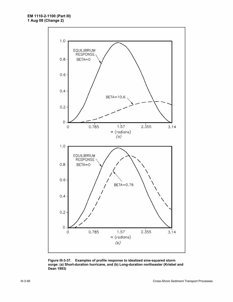
EM 1110-2-1100 (Part III)1 Aug 08 (Change 2)
III-3-56 Cross-Shore Sediment Transport Processes
Figure III-3-37. Examples of profile response to idealized sine-squared stormsurge: (a) Short-duration hurricane, and (b) Long-duration northeaster (Kriebel andDean 1993)

EM 1110-2-1100 (Part III)1 Aug 08 (Change 2)
Cross-Shore Sediment Transport Processes III-3-57
Figure III-3-38. Maximum relative erosion versus ratio of storm duration toprofile time scale, TD/TS
Figure III-3-39. Empirical relationship for determination of erosion time scale,Ts

EM 1110-2-1100 (Part III)1 Aug 08 (Change 2)
III-3-58 Cross-Shore Sediment Transport Processes
EXAMPLE PROBLEM III-3-7FIND:
The shoreline recession, R(t), as a function of time and quantify the maximum erosion, Rmax.
GIVEN:Hb = 3 m, hb = 3.85m, D = 0.2 mm, B = 2 m, mo = 1:10, TD = 10 hr, and Smax = 1.5 m.
SOLUTION:
As in previous examples, the value of the profile scale parameter is determined from Figure III-3-18and/or Table III-3-3 as 0.1 m1/3. The active width of the surf zone Wb is calculated from Equation 3-19as
The equilibrium value of the shoreline response based on the maximum water level Smax is determinedfrom Equation 3-38 as
The morphological time scale Ts is determined from Figure III-3-39 by calculating the value of theabscissa in Figure III-3-39 as
(Continued)
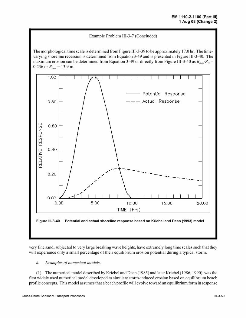
EM 1110-2-1100 (Part III)1 Aug 08 (Change 2)
Cross-Shore Sediment Transport Processes III-3-59
Figure III-3-40. Potential and actual shoreline response based on Kriebel and Dean (1993) model
Example Problem III-3-7 (Concluded)
The morphological time scale is determined from Figure III-3-39 to be approximately 17.0 hr. The time-varying shoreline recession is determined from Equation 3-49 and is presented in Figure III-3-40. Themaximum erosion can be determined from Equation 3-49 or directly from Figure III-3-40 as Rmax/R4 =0.236 or Rmax = 13.9 m.
very fine sand, subjected to very large breaking wave heights, have extremely long time scales such that theywill experience only a small percentage of their equilibrium erosion potential during a typical storm.
k. Examples of numerical models.
(1) The numerical model described by Kriebel and Dean (1985) and later Kriebel (1986, 1990), was thefirst widely used numerical model developed to simulate storm-induced erosion based on equilibrium beachprofile concepts. This model assumes that a beach profile will evolve toward an equilibrium form in response
EM 1110-2-1100 (Part III)1 Aug 08 (Change 2)
III-3-60 Cross-Shore Sediment Transport Processes
(III-3-53)
(III-3-54)
to changing water levels and wave conditions and that the sediment transport rate is proportional to the“disequilibrium” existing between the profile at any instant in time and the equilibrium profile form.
This is quantified in terms of the “excess” energy dissipation per unit volume in the surf zone, as given byEquation 3-45. The energy dissipation per unit volume at any location in the surf zone is given by
where the last form is based on the assumption of shallow-water breaking waves. Based on the equilibriumbeach profile given by Equation 3-14, the equilibrium energy dissipation per unit volume is given by
where the equilibrium profile parameter A is determined either from the sediment grain size, as suggested inTable III-3-3 or from a best-fit of the equilibrium profile equation h = Ay2/3 to the measured beach profile.
(2) The numerical solution for profile response is based on a finite difference solution to the sedimentconservation equation given in Equation 3-44. In this case, the profile is gridded in a “stair-step” form asshown in Figure III-3-36(b) so that erosion or accretion (retreat or advance) of each elevation contour isdetermined by vertical gradients in the sediment transport rate. At each time-step, the local depth h inEquation 3-53 is the depth to the sand bed below the time-varying storm surge. As a result, beach profilechange is driven primarily by changes in water level associated with storm surge. Breaking waves are treatedvery simply by shallow-water, spilling-breaker assumptions and, as a result, have a secondary effect onprofile response. In effect, the breakpoint serves to separate the two main computational domains in themodel: the offshore region, where the sediment transport rate is assumed to equal zero, and the surf zone,where the transport rate is given by Equation III-3-45.
(3) In this model, an increase in water level due to storm surge allows waves to break closer to shore,thus temporarily decreasing the width of the surf zone and increasing the energy dissipation per unit volumeabove the equilibrium level. According to Equation III-3-45, this leads to offshore directed sediment trans-port, the gradients of which cause erosion of the foreshore, deposition near the breakpoint, and an overallwidening of the profile toward a new equilibrium form. At each time-step in the finite-difference solution,the profile responds toward equilibrium, but this is rarely, if ever, achieved due to the limited storm durations.
(4) The transport relationship used in the Kriebel and Dean model, given by Equation 3-45, requirescalibration of a single empirical parameter KN. Kriebel (1986) first determined this parameter from numericalsimulations of both large wave tank tests and hurricane-induced beach profile change as observed inHurricane Eloise on the Gulf Coast of Florida. Figure III-3-41 shows numerical profile development alongwith results of large wave tank tests of Saville (1957). This illustrates the time-dependent profiledevelopment. It is noted that in the offshore region near the breakpoint, numerical results appear reasonable;however, the model does not simulate bar and trough features. For the Hurricane Eloise data, one profile wascalibrated and the calibrated model was then applied to 20 additional profiles. Overall results showed thatthe model was capable of predicting the volume eroded from the dune to within about 25 to 40 percent, withlittle bias toward either under- or overestimating the volume eroded. Figure III-3-42 shows numerical modelsimulation of a long-duration extra-tropical storm from Point Pleasant, New Jersey. In these cases, measured
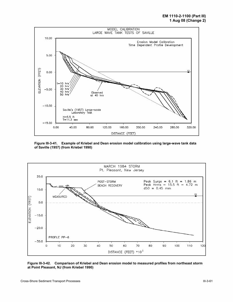
EM 1110-2-1100 (Part III)1 Aug 08 (Change 2)
Cross-Shore Sediment Transport Processes III-3-61
Figure III-3-41. Example of Kriebel and Dean erosion model calibration using large-wave tank dataof Saville (1957) (from Kriebel 1990)
Figure III-3-42. Comparison of Kriebel and Dean erosion model to measured profiles from northeast stormat Point Pleasant, NJ (from Kriebel 1990)
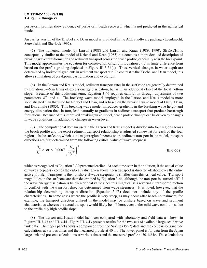
EM 1110-2-1100 (Part III)1 Aug 08 (Change 2)
III-3-62 Cross-Shore Sediment Transport Processes
(III-3-55)
post-storm profiles show evidence of post-storm beach recovery, which is not predicted in the numericalmodel.
An earlier version of the Kriebel and Dean model is provided in the ACES software package (Leenknecht,Szuwalski, and Sherlock 1992).
(5) The numerical model by Larson (1988) and Larson and Kraus (1989, 1990), SBEACH, isconceptually similar to the model of Kriebel and Dean (1985) but contains a more detailed description ofbreaking wave transformation and sediment transport across the beach profile, especially near the breakpoint.This model approximates the equation for conservation of sand in Equation 3-43 in finite difference formbased on the profile gridding depicted in Figure III-3-36(a). Thus, vertical changes in water depth aredetermined by horizontal gradients in sediment transport rate. In contrast to the Kriebel and Dean model, thisallows simulation of breakpoint bar formation and evolution.
(6) In the Larson and Kraus model, sediment transport rates in the surf zone are generally determinedby Equation 3-46 in terms of excess energy dissipation, but with an additional effect of the local bottomslope. Because of this additional term, Equation 3-46 requires calibration through adjustment of twoparameters, KNN and ,. The breaking wave model employed in the Larson and Kraus model is moresophisticated than that used by Kriebel and Dean, and is based on the breaking wave model of Dally, Dean,and Dalrymple (1985). This breaking wave model introduces gradients in the breaking wave height andenergy dissipation that, in turn, lead naturally to gradients in sediment transport that produce bar/troughformations. Because of this improved breaking wave model, beach profile changes can be driven by changesin wave conditions, in addition to changes in water level.
(7) The computational domain used in the Larson and Kraus model is divided into four regions acrossthe beach profile and the exact sediment transport relationship is adjusted somewhat for each of the fourregions. In the surf zone, which is the major region for cross-shore sediment transport in the model, transportdirections are first determined from the following critical value of wave steepness
which is recognized as Equation 3-30 presented earlier. At each time-step in the solution, if the actual valueof wave steepness exceeds the critical value given above, then transport is directed offshore over the entireactive profile. Transport is then onshore if wave steepness is smaller than this critical value. Transportmagnitudes in the surf zone are then determined by Equation 3-44, although the transport is “turned off” ifthe wave energy dissipation is below a critical value since this might cause a reversal in transport directionin conflict with the transport direction determined from wave steepness. It is noted, however, that therelationship determining transport direction (Equation 3-53) does not include any of the profilecharacteristics. In some cases where the profile is very steep, as may occur after beach nourishment, forexample, the transport direction utilized in the model may be onshore based on wave and sedimentcharacteristics whereas the actual transport would likely be offshore, even under mild wave conditions, dueto the artificially high profile slope.
(8) The Larson and Kraus model has been compared with laboratory and field data as shown inFigures III-3-43 and III-3-44. Figure III-3-43 presents results for the two sets of available large-scale wavetank data. The upper panel shows a comparison from the Saville (1957) data and the comparisons includecalculations at various times and the measured profile at 40 hr. The lower panel is for data from the Japanlarge tank and presents calculations at various times and the measured profile at 30-1/2 hr. The calculations

EM 1110-2-1100 (Part III)1 Aug 08 (Change 2)
Cross-Shore Sediment Transport Processes III-3-63
Figure III-3-43. SBEACH compared to two tests from large-scale wave tanks (Larson and Kraus1989)

EM 1110-2-1100 (Part III)1 Aug 08 (Change 2)
III-3-64 Cross-Shore Sediment Transport Processes
Figure III-3-44. SBEACH tested against profile evolution data from Duck, NC (Larson and Kraus1989)
EM 1110-2-1100 (Part III)1 Aug 08 (Change 2)
Cross-Shore Sediment Transport Processes III-3-65
(III-3-56)
(III-3-57)
(III-3-58)
(III-3-59)
are in quite good agreement with the data. The regular waves used in these tests were monochromatic, whichtend to favor the well-developed and concentrated bars that are simulated quite well by the numerical model.Figure III-3-44, from Duck, NC, compares the evolution of a profile over a 3-day period in which the waveheights were on the order of 1.5 m. The initial profile included a bar located approximately 40 m fromshore. During the period of interest, the bar migrated seaward approximately 65 m. The simulations providea reasonable qualitative representation of the evolution. The bar becomes more subdued at its initiallocation, but in contrast to measurements , is still present at the final time. Also, the bar had started toemerge slightly seaward of the measured location. The calculations showed substantially greater erosion atthe shoreline than measured. This example demonstrates the extreme difficulty in simulating an actual eventin nature. In the SBEACH model, sediment transport rates from Equation 3-46 require calibration throughadjustment of two parameters, KNN and ,.
l. Physical modeling of beach profile response.
(1) Physical modeling of beach profile response is carried out with the model being a scaled version ofthe prototype. In recent years, physical modelling of profiles has been employed predominantly as a researchmethod to understand transport processes rather than as a means to investigate profile response to a particularscenario of water level and wave conditions. The ratio of quantities in the model to those in the prototypeis termed the “scale ratio” and will be designated here by a subscript “r.” For example, the length and waveperiod ratios would be Lr and Tr, respectively. In some models, it is appropriate to utilize a distorted modelin which the vertical scale ratio is different from that of the horizontal scale. Modelling of cross-shoresediment transport requires the determination of the appropriate scaling relationships for both the waves andsediments. Hughes (1994) presents a complete discussion of scaling laws as applied to predicting cross-shoresediment transport.
(2) Noda (1972) carried out a study of profile modelling and has found that distorted models wereappropriate. The horizontal and vertical scale ratios were recommended as
in which Dr is the grain size ratio, sr is the submerged specific weight ratio, sr = ((Ds - D)/D)r in which Ds andD are the mass density of sediment and water, respectively, lr is the horizontal length scale, and hr is the verti-cal length ratio. Figure III-3-45 presents Noda's recommended scaling relationships. Usually sand is thecommon material in both the model and prototype, Ds = 2650 kg/m3, and Equation III-3-56 and III-3-57become
and

EM 1110-2-1100 (Part III)1 Aug 08 (Change 2)
III-3-66 Cross-Shore Sediment Transport Processes
Figure III-3-45. Noda's recommendation for profile modeling (Noda 1972)
(III-3-60)
(3) Thus, according to Noda's relationships, the diameter would be scaled in accordance with the depthratio; however, the scaling factor for diameter would be closer to unity than that for the depth ratio and thelength ratio would be smaller than the depth ratio. This type of distortion is common for hydraulic modelsin which it is necessary to represent a large horizontal extent.
(4) Dean (1973) carried out a study of conditions that would lead to bar formation and suggested thatthe fall time of a sediment particle suspended at the wave crest phase position relative to the wave periodwould be relevant in modelling applications. This led Dean (1973, 1985) to identify the followingcombination of parameters which should be maintained the same in model and prototype

EM 1110-2-1100 (Part III)1 Aug 08 (Change 2)
Cross-Shore Sediment Transport Processes III-3-67
(III-3-61)
(III-3-62)
(5) This combination of terms will be termed herein as the “Fall Velocity Parameter” (FVP). It wasfurther suggested that an appropriate model for cross-shore sediment transport is one based on undistortedFroude modelling for the wave characteristics and one that maintains the FVP the same in the model andprototype. This simple approach leads to the following requirement for scaling the sediment fall velocity wf
which is the standard relationship for velocity scaling for a Froude model.
(6) Evaluation of cross-shore modelling according to the FVP has been carried out by Vellinga (1983),Kriebel, Dally, and Dean (1986) and Hughes and Fowler (1990). Each of these studies concluded that theFVP was effective in scaling the erosion process. Figures III-3-46 and III-3-47, from Kriebel, Dally, andDean (1986) and Hughes and Fowler (1990), compare different scales while maintaining the same FVP inmodel and prototype. Considering the FVP as valid leads to the following valuable transport relationship fornumerical models
(7) One limitation for scaling by the FVP is that the length ratio Lr and the prototype diameter can resultin designated model sediments so small that cohesive forces would be significant. Although there are no strictguidelines for a minimum sediment size, values smaller than approximately 0.08 to 0.09 mm should beavoided.
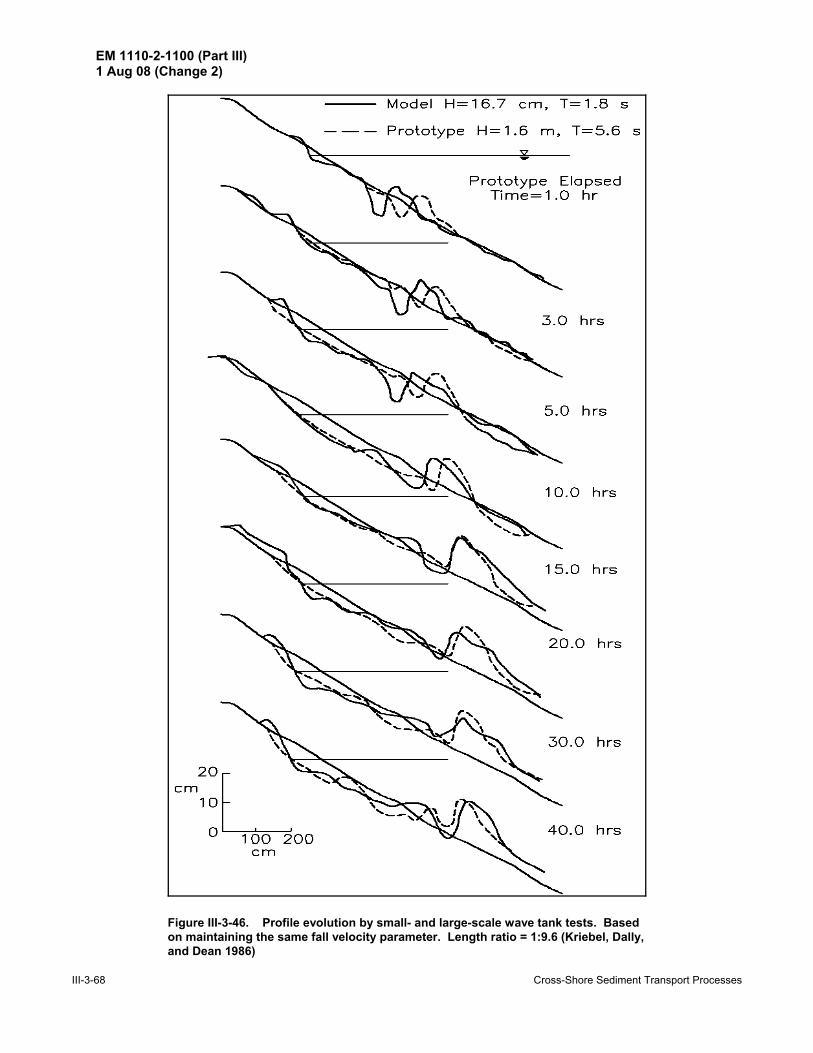
EM 1110-2-1100 (Part III)1 Aug 08 (Change 2)
III-3-68 Cross-Shore Sediment Transport Processes
Figure III-3-46. Profile evolution by small- and large-scale wave tank tests. Basedon maintaining the same fall velocity parameter. Length ratio = 1:9.6 (Kriebel, Dally,and Dean 1986)

EM 1110-2-1100 (Part III)1 Aug 08 (Change 2)
Cross-Shore Sediment Transport Processes III-3-69
Figure III-3-47. Profile evolution by small- and large-scale wave tank tests. Case of sloping seawall. Basedon maintaining the same fall velocity parameter. Length ratio = 1:7.5 (Hughes and Fowler 1990)
III-3-4. References
Bagnold 1940Bagnold, R. A. 1940. “Beach Formation by Waves: Some Model Experiments in a Wave Tank,” Journalof the Institution of Civil Engineers, Vol 15, pp 27-52.
Bagnold 1966Bagnold, R. A. 1966. “An Approach to the Sediment Transport Problem from General Physics,”U.S. Geological Survey Professional Paper 422-I, U. S. Dept of Interior.
Bailard 1981Bailard, J. A. 1981. “An Energetics Total Load Sediment Transport Model for a Plane Sloping Beach,”Journal of Geophysical Research, Vol 86, No. C11, pp 10938-10954.
Barnett and Wang 1988Barnett, M., and Wang, H. 1988. “Effects of a Vertical Seawall on Profile Response,” American Society ofCivil Engineers, Proceedings of the Twenty-first International Conference on Coastal Engineering,Chapter 111, pp 1493-1507.

EM 1110-2-1100 (Part III)1 Aug 08 (Change 2)
III-3-70 Cross-Shore Sediment Transport Processes
Birkemeier 1984Birkemeier, W. A. 1984. “Time Scales of Nearshore Profile Change,” Proceedings, 19th InternationalConference on Coastal Engineering, Chapter 102, pp 1501-1521.
Birkemeier 1985Birkemeier, W. A. 1985. “Field Data on Seaward Limit of Profile Change,” Journal of the Waterways, PortCoastal and Ocean Engineering, American Society of Civil Engineers, Vol 111, No. 3, pp 598-602.
Bodge 1992Bodge, K. R. 1992. “Representing Equilibrium Beach Profiles with an Exponential Expression,” Journal ofCoastal Research, Vol 8, No. 1, pp 47-55.
Broker-Hedegaard, Deigaard, and Fredsoe 1991Broker-Hedegaard, I., Deigaard, R., and Fredsoe, J. 1991. “Onshore/Offshore Sediment Transport andMorphological Modelling of Coastal Profiles,”Proceedings Coastal Sediments '91 Conference, pp 643-657.
Bruun 1954Bruun, P. 1954. “Coast Erosion and the Development of Beach Profiles,” Beach Erosion Board TechnicalMemorandum No. 44, U.S. Army Engineer Waterways Experiment Station, Vicksburg, MS.
Bruun 1962Brunn, P. 1962. “Sea-Level Rise as a Cause of Shore Erosion,” Journal of Waterways and Harbor Division,American Society of Civil Engineers, Vol 88, pp 117-130.
Bruun 1988Bruun, P. 1988. “The Bruun Rule of Erosion by Sea Level Rise: A Discussion on Large-Scale Two- andThree-Dimensional Usages,” Journal of Coastal Research, Vol 4, No. 4, pp 627-648.
Chiu 1977Chiu, T. Y. 1977. “Beach and Dune Response to Hurricane Eloise of September 1975. Proceedings ofCoastal Sediments '77, pp 116-134.
Clausner, Birkemeier, and Clark 1986Clausner, J. E., Birkemeier, W. A., and Clark, G. R. 1986. “Field Comparison of Four Nearshore SurveySystems,” Miscellaneous Paper CERC-86-6, U.S. Army Engineer Waterways Experiment Station, Vicksburg,MS.
Dally and Dean 1984Dally, W. R., and Dean, R. G. 1984. “Suspended Sediment Transport and Beach Profile Evolution,” Journalof Waterway, Port, Coastal, and Ocean Engineering, Vol 110, No. 1, pp 15-33.
Dally, Dean, and Dalrymple 1985Dally, W. R., Dean, R. G., and Dalrymple, R. G. 1985. “Wave Height Variation Across Beaches of ArbitraryProfile,” Journal of Geophysical Research, Vol 90, No. C6, pp 11917-11927.
Dalrymple 1992Dalrymple, R. A. 1992. “Prediction of Storm/Normal Beach Profiles,” Journal of Waterways, Port, Coastaland Ocean Engineering, American Society of Civil Engineers, Vol 118, No. 2, pp 193-200.

EM 1110-2-1100 (Part III)1 Aug 08 (Change 2)
Cross-Shore Sediment Transport Processes III-3-71
Dean 1973Dean, R. G. 1973. “Heuristic Models of Sand Transport in the Surf Zone,” Proceedings, Conference onEngineering Dynamics in the Surf Zone, Sydney, Australia.
Dean 1977Dean, R. G. 1977. “Equilibrium Beach Profiles: U.S. Atlantic and Gulf Coasts,” Department of CivilEngineering, Ocean Engineering Report No. 12, University of Delaware, Newark, DE.
Dean 1985Dean, R. G. 1985. “Physical Modelling of Littoral Processes,” Physical Modelling in Coastal Engineering,R. A. Dalrymple, ed., A. A. Balkema, pp 119-139.
Dean 1987aDean, R. G. 1987a. “Additional Sediment Input into the Nearshore Region,” Shore and Beach, Vol 55,Nos. 3-4, pp 76-81.
Dean 1987bDean, R. G. 1987b. “Coastal Sediment Processes: Toward Engineering Solutions,” Coastal Sediments '87,American Society of Civil Engineers, New Orleans, LA, Vol 1, pp 1-24.
Dean 1991Dean, R. G. 1991. “Equilibrium Beach Profiles: Characteristics and Applications,” Journal of CoastalResearch, Vol 7, No. 1, pp 53-84.
Dean and Dalrymple 1991Dean, R. G., and Dalrymple, R. A. 1991. Water Wave Mechanics for Engineers and Scientists, WorldScientific Pub. Co., Teaneck, NJ.
Dean and Dalrymple 2001Dean, R. G., and Dalrymple, R. A. 2001. Coastal Processes with Engineering Applications, CambridgeUniversity Press, New York.
Dean and Maurmeyer 1983Dean, R. G., and Maurmeyer, E. M. 1983. “Models for Beach Profile Response,” CRC Handbook on BeachErosion and Coastal Processes, P. D. Komar, ed., Chapter 7, pp 151-166.
Dette and Uliczka 1987Dette, H., and Uliczka, K. 1987. “Prototype Investigation on Time-Dependent Dune Recession and BeachErosion,” Proceedings Coastal Sediments '87, New Orleans, pp 1430-1444.
Dewall 1979Dewall, A. E. 1979. “Beach Changes at Westhampton Beach, New York,” MR 79-5, Coastal EngineeringResearch Center, U.S. Army Engineer Waterways Experiment Station, Vicksburg, MS.
Dewall and Richter 1977Dewall, A. E., and Richter, J. J. 1977. “Beach and Nearshore Processes in Southeastern Florida,” CoastalSediments'77, pp 425-443.

EM 1110-2-1100 (Part III)1 Aug 08 (Change 2)
III-3-72 Cross-Shore Sediment Transport Processes
Dolan and Dean 1985Dolan, T., and Dean, R. G. 1985. “Multiple Longshore Sand Bars in the Upper Chesapeake Bay,” EstuarineCoastal & Shelf Science, Vol 21, pp 727-743.
Edelman 1972Edelman, T. 1972. “Dune Erosion During Storm Conditions,” Proceedings of the Thirteenth InternationalConference on Coastal Engineering, pp 1305-1312.
Everts 1985Everts, C. H. 1985. “Sea Level Rise Effects on Shoreline Position,” Journal of Waterway, Port, and CoastalEngineering, Vol 111, No. 6, pp 985-999.
Hallermeier 1978Hallermeier, R. J. 1978. “Uses for a Calculated Limit Depth to Beach Erosion,” Proceedings of the 16thInternational Conference on Coastal Engineering, American Society of Civil Engineers, Hamburg, pp 1493-1512.
Hallermeier 1981Hallermeier, R. J. 1981. “A Profile Zonation for Seasonal Sand Beaches from Wave Climate,” CoastalEngineering, Vol 4, pp 253-277.
Hands 1983Hands, E. 1983. “Erosion of the Great Lakes Due to Changes in the Water Level,” CRC Handbook ofCoastal Processes and Erosion, P. D. Komar, ed., CRC Press, pp 167-189.
Hicks, Debaugh, and Hickman 1983Hicks, S. D., Debaugh, H. A., Jr., and Hickman, E. 1983. “Sea Level Variations for the United States, 1955-1980,” National Ocean Service, National Oceanic and Atmospheric Administration.
Hughes 1994Hughes, S. A. 1994. Physical Models and Laboratory Techniques in Coastal Engineering. World Scientific,River Edge, NJ.
Hughes and Fowler 1990Hughes, S. A., and Fowler, J. E. 1990. “Validation of Movable-Bed Modeling Guidance,” Proceedings ofthe 22nd International Conference on Coastal Engineering, American Society of Civil Engineers, Chapter186, pp 2457-2470.
Inman, Elwany, and Jenkkins 1993Inman, D. L., Elwany, M. H. S., and Jenkkins, S. A. 1993. “Shoreline and Bar-Berm Profiles on OceanBeaches,” Journal of Geophysical Research, Vol 98, No. C10, pp 18,181 - 18,199.
Katoh and Yanagishima 1988Katoh, K., and Yanagishima, S. 1988. “Predictive Model for Daily Changes of Shoreline,” Proceedings ofthe Twenty-First International Conference on Coastal Engineering, American Society of Civil Engineers,Hamburg, Chapter 93, pp 1253-1264.
EM 1110-2-1100 (Part III)1 Aug 08 (Change 2)
Cross-Shore Sediment Transport Processes III-3-73
Keulegan 1945Keulegan, G. H. 1945. “Depths of Offshore Bars,” Engineering Notes No. 8, Beach Erosion Board,U.S. Army Engineer Waterways Experiment Station, Vicksburg, MS.
Keulegan 1948Keulegan, G. H. 1948. “An Experimental Study of Submarine Sand Bars,” Technical Report No. 8, BeachErosion Board, U.S. Army Engineer Waterways Experiment Station, Vicksburg, MS.
Kobayashi 1987Kobayashi, N. 1987. “Analytical Solutions for Dune Erosion by Storms,” Journal of the Waterway, Coastaland Ocean Engineering, American Society of Civil Engineers, Vol 113, No. 4, pp 401-418.
Komar and McDougal 1994Komar, P. D., and McDougal, W. G. 1994. “The Analysis of Exponential Beach Profiles,” Journal ofCoastal Research, Vol 10, pp 59-69.
Kraus 1988Kraus, N. C. 1988. “The Effects of Seawalls on the Beach: An Extended Literature Review,” Journal ofCoastal Research, Special Issue No. 4, pp 1-28.
Kraus, Larson, and Kriebel 1991Kraus, N. C., Larson, M., and Kriebel, D. L. 1991. “Evaluation of Beach Erosion and Accretion Predictors,”Proceedings of Conference on Coastal Sediments '91, American Society of Civil Engineers, pp 572-587.
Kriebel 1986Kriebel, D. L. 1986. “Verification Study of a Dune Erosion Model,” Shore and Beach, Vol 54, No. 3,pp 13-20.
Kriebel 1987Kriebel, D. L. 1987. “Beach Recovery Following Hurricane Elena,” Proceedings of Conference on CoastalSediments '87, American Society of Civil Engineers, pp 990-1005.
Kriebel 1990Kriebel, D. L. 1990. “Advances in Numerical Modeling of Dune Erosion,” 22nd Intl. Conf. on CoastalEngineering, American Society of Civil Engineers, pp 2304-2317.
Kriebel and Dean 1985Kriebel, D. L., and Dean, R. G. 1985. “Numerical Simulation of Time-Dependent Beach and Dune Erosion,”Coastal Engineering, Vol 9, pp 221-245.
Kriebel and Dean 1993Kriebel, D. L., and Dean, R. G. 1993. “Convolution Method for Time-Dependent Beach-Profile Response,”Journal of Waterway, Port, Coastal and Ocean Engineering, American Society of Civil Engineers, Vol 119,No. 2, pp 204-227.
Kriebel, Dally, and Dean 1986Kriebel, D. L., Dally, W. R., and Dean, R. G. 1986. “Undistorted Froude Model for Surf Zone SedimentTransport,” Proceedings of the Twentieth International Conference on Coastal Engineering, AmericanSociety of Civil Engineers, pp 1296-1310.

EM 1110-2-1100 (Part III)1 Aug 08 (Change 2)
III-3-74 Cross-Shore Sediment Transport Processes
Kriebel, Kraus, and Larson 1991Kriebel, D. L., Kraus, N. C., and Larson, M. 1991. “Engineering Methods for Predicting Beach ProfileResponse,” Proceedings of Conference on Coastal Sediments '91, American Society of Civil Engineers,pp 557-571.
Larson 1988Larson, M. 1988. “Quantification of Beach Profile Change,” Report No. 1008, Department of WaterResources and Engineering, University of Lund, Lund, Sweden.
Larson and Kraus 1989Larson, M., and Kraus, N. C. 1989. “SBEACH: Numerical Model for Simulating Storm-induced BeachChange; Report 1: Empirical Foundation and Model Development,” Technical Report CERC-89-9,U.S. Army Engineer Waterways Experiment Station, Vicksburg, MS.
Larson and Kraus 1990Larson, M., and Kraus, N. C. 1990. “SBEACH: Numerical Model for Simulating Storm-induced BeachChange; Report 2: Numerical Formulation and Model Tests,” Technical Report CERC-89-9, U.S. ArmyEngineer Waterways Experiment Station, Vicksburg, MS.
Lee and Birkemeier 1993Lee, G. H., and Birkemeier, W. A. 1993. “Beach and Nearshore Survey Data: 1985-1991 CERC FieldResearch Facility,” Technical Report CERC-93-3, U.S. Army Engineer Waterways Experiment Station,Vicksburg, MS.
Leenknecht, Szuwalski, and Sherlock 1992Leenknecht, D. A., Szuwalski, A., and Sherlock, A. R. 1992. “Automated Coastal Engineering System, UserGuide and Technical Reference, Version 1.07,” U.S. Army Engineer Waterways Experiment Station,Vicksburg, MS.
Longuet-Higgins 1953Longuet-Higgins, M. S. 1953. “Mass Transport in Water Waves,” Philosophical Transactions of the RoyalSociety of London, Ser A, Vol 245, pp 535-581.
Longuet-Higgins and Stewart 1964Longuet-Higgins, M. S., and Stewart, R. W. 1964. “Radiation Stresses in Water Waves: A PhysicalDiscussion with Applications,” Deep Sea Research, Vol 2, pp 529-562.
Moore 1982Moore, B. D. 1982. “Beach Profile Evolution in Response to Changes to Water Level and Wave Height,”M.S. thesis, Department of Civil Engineering, University of Delaware, Newark.
Nairn and Southgate 1993Nairn, R. B., and Southgate, H. N. 1993. “Deterministic Profile Modelling of Nearshore Processes; Part 2,Sediment Transport and Beach Profile Development,” Coastal Engineering, Vol 19, pp 57-96.
National Research Council 1984National Research Council. 1984. “Responding to Changes in Sea Level: Engineering Implications,”National Research Council Committee on Engineering Implication of Change in Relative Sea Level.

EM 1110-2-1100 (Part III)1 Aug 08 (Change 2)
Cross-Shore Sediment Transport Processes III-3-75
Noda 1972Noda, E. K. 1972. “Equilibrium Beach Profile Scale Model Relationships,” Journal of Waterway, Harborsand Coastal Engineering, American Society of Civil Engineers, Vol 98, No. 4, pp 511-528.
Penland, Suter, and McBride 1987Penland, S., Suter, J. R., and McBride, R. A. 1987. “Delta Plain Development and Sea Level History inTerrebonne Coastal Region, Louisiana,” Proceedings of Conference on Coastal Sediments '87, AmericanSociety of Civil Engineers, pp 1689-1705.
Roelvink and Broker 1993Roelvink, J. A., and Broker, I. 1993. “Cross-Shore Profile Models,” Coastal Engineering, Vol 21, pp 163-191.
Roelvink and Stive 1989Roelvink, J. A., and Stive, M. J. F. 1989. “Bar Generating Cross-Shore Flow Mechanisms on a Beach,”Journal of Geophysical Research, Vol 94, No. C4, pp 4785-4800.
Saville 1957Saville, T. 1957. “Scale Effects in Two-Dimensional Beach Studies,” Transactions of the Seventh GeneralMeeting of the International Association of Hydraulic Research, Vol 1, pp A3.1 - A3.10.
Seymour and Boothman 1984Seymour, R. J., and Boothman, D. P. 1984. “A Hydrostatic Profiler for Nearshore Surveying,” Journal ofCoastal Engineering, Vol 8, pp 1-14.
Stive and Battjes 1984Stive, M. J. F., and Battjes, J. A. 1984. “A Model for Offshore Sediment Transport,” Proceedings 19th Intl.Conf. on Coastal Engineering, pp 1420-1436.
Swart 1974Swart, D. H. 1974. “Offshore Sediment Transport and Equilibrium Beach Profiles,'' Publ. No. 131, DelftHydraulics Lab, Delft, The Netherlands.
Vellinga 1983Vellinga, P. 1983. “Predictive Computational Model for Beach and Dune Erosion During Storm Surges,”Proceedings, American Society of Civil Engineers Specialty Conference on Coastal Structures' 83, pp 806-819.
Watanabe, Riho, and Horikawa 1980Watanabe, A., Riho, Y., and Horikawa, K. 1980. “Beach Profile and On-Offshore Sediment Transport,”Proceedings 17th International Conference on Coastal Engineering, pp 1106-1121.

EM 1110-2-1100 (Part III)1 Aug 08 (Change 2)
III-3-76 Cross-Shore Sediment Transport Processes
III-3-5. Definition of Symbols
$ Ratio of the erosion time scale to the storm duration [dimensionless]
)y Equilibrium dry beach width [length]
)yN Non-dimensional equilibrium dry beach width
g Parameter suggested by Larson & Kraus to calibrate a sediment transport model[dimensionless]
g Eddy viscosity [length2/time]
6 Ratio of wave height to local depth within the surf zone
<b Instantaneous wave-induced water particle velocity at the bottom [length/time]
<s Steady wave-induced water particle velocity [length/time]
D Mass density of water (salt water = 1,025 kg/m3 or 2.0 slugs/ft3; fresh water =1,000kg/m3 or 1.94 slugs/ft3) [force-time2/length4]
F Angular frequency (= 2B/T) [time-1]
FH Standard deviation of significant wave height [length]
J&b Average bottom shear stress [force/length2]
J&bs Bottom shear stress [force/length2]
J0 Surface wind stress [force/length2]
Jb Seaward-directed shear stress at the bottom [force/length2]
A Sediment scale or equilibrium profile parameter (Table III-3-3) [length1/3]
AF Nourishment material scale parameter [length1/3]
AN Native sediment scale parameter [length1/3]
AN Parameter for nourished beach calculations ( = AF / AN ) [dimensionless]
B Berm height [length]
B(t) Instantaneous total height of the active profile above the current water level [length]
B0 Original berm height [length]
BN Parameter for nourished beach calculations [dimensionless]
C Wave speed [length/time]
D Sediment grain diameter [length - generally millimeters]
D* Excess energy dissipation per unit volume in the surf zone
DF Sediment grain diameter of beach fill material [length - generally millimeters]
DN Sediment grain diameter of native beach [length] - generally millimeters
Dr Model to prototype sediment grain size scale ratio

EM 1110-2-1100 (Part III)1 Aug 08 (Change 2)
Cross-Shore Sediment Transport Processes III-3-77
E Total wave energy in one wavelength per unit crest width [length-force/length]
f Darcy-Weisbach friction coefficient [dimensionless]
g Gravitational acceleration (32.17 ft/sec2, 9.807m/sec2) [length/time2]
h Equilibrium beach profile depth (Equation III-3-13) [length]
h Water depth [length]
H Wave height [length]
h* Depth to which nourished profile will equilibrate or closure depth [length]
H& Annual mean significant wave height [length]
h0 Asymptotic beach profile depth [length]
H0 Deepwater wave height [length]
hb Breaking depth [length]
hc Closure depth [length]
hCR Depth over bar crest [length]
hD Depth to the bar base [length]
He Effective significant wave height [length]
hr Model to prototype vertical length scale ratio
Hs Deepwater significant wave height [length]
hT Depth over bar trough [length]
k Decay constant [dimensionless]
k Wave number (= 2B/L = 2B/CT) [length-1]
KN Parameter used to calibrate the Kriebel & Dean simple transport relationship[dimensionless]
KNN Parameter used to calibrate a sediment transport model [dimensionless]
L* Width of active profile [length]
L0 Deepwater wave length [length]
lr Model to prototype horizontal length scale ratio
Lr Model to prototype length scale ratio
m0 Beach slope [length-rise/length-run]
n Empirical exponent used in the equilibrium beach profile equation [dimensionless]
P Single profile parameter (Equation III-3-32) [dimensionless]
Q Time-averaged seaward discharge due to the return flow of shoreward masstransport

EM 1110-2-1100 (Part III)1 Aug 08 (Change 2)
III-3-78 Cross-Shore Sediment Transport Processes
qy Kriebel & Dean simple transport relationship (Equation III-3-45)
R Shoreline recession [length]
Rmax Maximum shoreline recession [length]
R4 Equilibrium berm recession due to a storm surge (Equation III-3-38) [length]
S Storm surge level [length]
S Sea level rise [length]
sr Model to prototype submerged specific weight scale ratio
T Wave period [time]
TD Total storm surge duration [time]
Te Effective wave period [time]
Tr Model to prototype wave period scale ratio
TS Time-scale of the equilibrium beach response system (Equation III-3-52) [time]
V Added volume per unit beach length [length3 /length]
V4 Volume of sand eroded from the berm above the initial still-water level due to astorm surge level S [length3/length]
VN Parameter for nourished beach calculations ( = V/(B W*) ) [dimensionless]
VNc2 Critical volume of sand that will just yield a finite shoreline displacement for thecase of sand that is finer than the native (Equation III-3-23) [dimensionless]
VNcl Critical volume of sand delineating intersecting and nonintersecting profiles(Equation III-3-22) [dimensionless]
w Sediment fall velocity [length/time]
W* Width of active nearshore zone (Equation III-3-19) [length]
Wb Width of the surf zone [length]
wf Sediment fall velocity [length/time]
y Equilibrium beach profile distance offshore (Equation III-3-13) [length]
y Distance seaward from mean low water [length]
y0 Offset of the shoreline between the sloping beach face and the imaginary or virtualorigin of the equilibrium profile [length]
z Elevation [length]

EM 1110-2-1100 (Part III)1 Aug 08 (Change 2)
Cross-Shore Sediment Transport Processes III-3-79
III-3-6. Acknowledgments
Authors of Chapter III-3, “Cross-Shore Sediment Transport Processes:”
Robert G. Dean, Ph.D., Coastal & Oceanographic Engineering, University of Florida, Gainesville, Florida.David L. Kriebel, Ph.D., Department of Ocean Engineering, United States Naval Academy, Annapolis,
Maryland.Todd L. Walton, Ph.D., Coastal and Hydraulics Laboratory, Engineer Research and Development Center,
Vicksburg, Mississippi.
Reviewers:Kevin Bodge, Ph.D., Olsen Associates, Jacksonville, Florida.James R. Houston, Ph.D., Engineer Research and Development Center, Vicksburg, Mississippi.Paul A. Work, Ph.D., School of Civil and Environmental Engineering, Georgia Institute of Technology,
Atlanta, Georgia.


![[1] Aagaard, Troels; Greenwood, Brian; Nielsen, Jorgen · [1] Aagaard, Troels; Greenwood, Brian; Nielsen, Jorgen: Cross-Shore Sediment Transport: A Field Test of the Bailard Energetics](https://img.pdfslide.net/doc/110x75/5b59407d7f8b9a655d8d0c5d/1-aagaard-troels-greenwood-brian-nielsen-1-aagaard-troels-greenwood.jpg)