Cross-Validation for Selecting a Model Selection Procedure∗

Yongli Zhang

LundQuist College of Business

University of Oregon

Eugene, OR 97403

Yuhong Yang

School of Statistics

University of Minnesota

Minneapolis, MN 55455

Abstract

While there are various model selection methods, an unanswered but important question is how to select one

of them for data at hand. The difficulty is due to that the targeted behaviors of the model selection procedures

depend heavily on uncheckable or difficult-to-check assumptions on the data generating process. Fortunately, cross-

validation (CV) provides a general tool to solve this problem. In this work, results are provided on how to apply CV

to consistently choose the best method, yielding new insights and guidance for potentially vast amount of application.

In addition, we address several seemingly widely spread misconceptions on CV.

Key words: Cross-validation, cross-validation paradox, data splitting ratio, adaptive procedure selection, information

criterion, LASSO, MCP, SCAD

1 Introduction

Model selection is an indispensable step in the process of developing a functional prediction model

or a model for understanding the data generating mechanism. While thousands of papers have been

published on model selection, an important and largely unanswered question is: How do we select

a modeling procedure that typically involves model selection and parameter estimation? In a real

application, one usually does not know which procedure fits the data the best. Instead of staunchly

following one’s favorite procedure, a better idea is to adaptively choose a modeling procedure. In

1

this article we focus on selecting a modeling procedure in the regression context through cross-

validation when, for example, it is unknown whether the true model is finite or infinite dimensional

in classical setting or if the true regression function is a sparse linear function or a sparse additive

function in high dimensional setting.

Cross-validation (e.g., Allen, 1974; Stone, 1974; Geisser, 1975) is one of the most commonly

used methods of evaluating predictive performances of a model, which is given a priori or developed

by a modeling procedure. Basically, based on data splitting, part of the data is used for fitting each

competing model and the rest of the data is used to measure the predictive performances of the

models by the validation errors, and the model with the best overall performance is selected. On

this ground, cross-validation (CV) has been extensively used in data mining for the sake of model

selection or modeling procedure selection (see, e.g., Hastie et al., 2009).

A fundamental issue in applying CV to model selection is the choice of data splitting ratio or

the validation size nv, and a number of theoretical results have been obtained. In the parametric

framework, i.e., the true model lies within the candidate model set, delete-1 (or leave-one-out,

LOO) is asymptotically equivalent to AIC (Akaike Information Criterion, Akaike, 1973) and they

are inconsistent in the sense that the probability of selecting the true model does not converge

to 1 as the sample size n goes to ∞, while BIC (Bayesian Information Criterion, Schwarz, 1978)

and delete-nv CV with nv/n → 1 (and n − nv → ∞) are consistent (see, e.g., Stone, 1977; Nishii,

1984; Shao, 1993). In the context of nonparametric regression, delete-1 CV and AIC lead to

asymptotically optimal or rate optimal choice for regression function estimation, while BIC and

delete-nv CV with nv/n → 1 usually lose the asymptotic optimality (Li, 1987; Speed and Yu,

1993; Shao, 1997). Consequently, the optimal choice of the data splitting ratio or the choice of an

information criterion is contingent on whether the data are under a parametric or a nonparametric

framework.

In the absence of prior information on the true model, an indiscriminate use of model selection

criteria may result in poor results (Shao, 1997; Yang, 2007a). Facing the dilemma in choosing

2

the most appropriate modeling or model selection procedure for the data at hand, CV provides a

general solution. A theoretical result is given on consistency of CV for procedure selection in the

traditional regression framework with fixed truth (Yang, 2007b).

In this article, in a framework of high-dimensional regression with possibly expanding true

dimension of the regression function to reflect the challenge of high dimension and small sample

size, we aim to investigate the relationship between the performance of CV and the data splitting

ratio in terms of modeling procedure selection instead of the usual model selection (which intends

to choose a model among a list of parametric models). Through theoretical and simulating studies,

we provide a guidance about the choice of splitting ratio for various situations. Simply speaking,

in terms of comparing the predictive performances of two modeling procedures, a large enough

evaluation set is preferred to account for the randomness in the prediction assessment, but at the

same time we must make sure that the relative performance of the two model selection procedures

at the reduced sample size resembles that at the full sample size. This typically forces the training

size to be not too small. Therefore, the choice of splitting ratio needs to balance the above two

conflicting directions.

The well-known conflict between AIC and BIC has attracted a lot of attention from both

theoretical and applied perspectives. While some researchers stick to their philosophy to strongly

favor one over the other, presumably most people are open to means to stop the “war”, if possible.

In this paper, we propose to use CV to share the strengths of AIC and BIC adaptively in terms

of asymptotic optimality. We show that an adaptive selection by CV between AIC and BIC on a

sequence of linear models leads to (pointwise) asymptotically optimal function estimation in both

parametric and nonparametric scenarios.

Two questions may immediately arise on the legitimacy of the approach we are taking. The

first is: If you use CV to choose between AIC and BIC that are applied on a list of parametric

models, you will end up with a model in that list. Since there is the GIC (Generalized Information

Criterion, e.g., Rao and Wu, 1989) that includes both AIC and BIC as special cases, why do you

3

take the more complicated approach? The second question is: Again, your approach ends up with

a model in the original list. Then why don’t you select one in the original list by CV directly? It

seems clear that your choosing between the AIC model and the BIC model by CV is much more

complicated. Our answers to these intriguing questions will be given in the conclusion section based

on the results we present in the paper.

Although CV is perhaps the most widely used tool for model selection, there are major seemingly

wide-spread misconceptions that may lead to improper data analysis. Some of these will be studied

as well.

The paper is organized as follows. In Section 2, we set up the problem and present the cross-

validation method for selecting a modeling procedure. The application of CV to share the strengths

of AIC and BIC is given in Section 3. In Section 4, a general result on consistency of CV in high-

dimensional regression is presented, with a few applications. In Sections 5 and 6, simulation results

and a real data example are given, respectively. In Section 7, we examine/discuss some issues with

misconceptions on CV. Concluding remarks are in Section 8. The proofs of the main results are in

the Appendix.

2 Cross validation to choose a modeling procedure

Suppose the data are generated by

Y = µ(X) + ε, (1)

where Y is the response, X comprises of pn features (X1, · · · , Xpn), µ(x) = E(Y |X = x) is the true

regression function and ε is the random error with E(ε|x) = 0 and E(ε2|x) <∞ almost surely. Let

(Xi, Yi)ni=1 denote n independent copies of (X1, · · · , Xpn , Y ). The distribution of Xi is unknown.

4

Consider regression models in the form of

µM (x) = β0 +∑j∈JM

βjφj(x), (2)

where M denotes a model structure, and in particular M may denote a subset of (X1, · · · , Xpn) if

only linear combinations of (X1, · · · , Xpn) (i.e., φj(x) = xj , j = 1, · · · , pn) are considered; and JM

is an index set associated with M . The statistical goal is to develop an estimator of µ(x) in the

form of (2) by a modeling procedure.

Cross validation is realized by splitting the data randomly into two disjoint parts: the training

set Zt = (Xi, Yi)i∈It consisting of nt sample points and the validating set Zv = (Xi, Yi)i∈Iv consist-

ing of the remaining nv observations, where It ∩ Iv = ϕ, It ∪ Iv = {1, · · · , n} and nt + nv = n. The

predictive performance of model M is evaluated by its validating error,

CV (M ; Iv) =1

nv

∑i∈Iv

(Yi − µIt,M (Xi)

)2, (3)

where µIt,M (x) is estimated based on the training set only. Let S be a collection of data splittings

at the same splitting ratio with |S| = S and s ∈ S denote a specific splitting, producing It(s) and

Iv(s). Usually the average validation error of multiple versions of data splitting

CV (M ;S) = 1

S

∑s∈S

CV (M ; Iv(s)) (4)

is considered to obtain a more stable assessment of the model’s predictive performance. This will

be called delete-nv CV error with S splittings for a given model, M . Note that there are different

ways to do this. One is to average over all possible data splittings, called leave-nv-out (Shao, 1993;

Zhang, 1993), which is often computationally infeasible. Alternatively, delete-nv CV can be carried

out through S (1 ≤ S <(nnv

)) splittings, and there are two slightly different approaches to average

over a randomly chosen subset of all possible data splittings, i.e., S: with or without replacement,

5

the former being called Monte Carlo CV (e.g., Picard and Cook, 1984) and the latter repeated

learning-testing (e.g., Breiman et al., 1984; Burman, 1989; Zhang, 1993). An even simpler version

is k-fold CV, in which case the data are randomly partitioned into k equal-size subsets. In turn each

of the k subsets is retained as the validation set, while the remaining k−1 folds work as the training

set, and the average prediction error of each candidate model is obtained. Hence, k-fold CV is one

version of delete-nv CV with nv = n/k and S = k. These different types of delete-nv CVs will be

studied theoretically and/or numerically in this paper. Although they may sometimes exhibit quite

different behaviors in practical uses, they basically share the same theoretical properties in terms

of selection consistency, as will be seen. We will call any of them a delete-nv CV for convenience

except when their differences are of interest. We refer to Arlot and Celisse (2010) for an excellent

and comprehensive review on cross-validation.

The new use of the CV, as is the focus in this work, is at the second level, i.e., the use of CV

to select a model selection procedure from a finite set of modeling procedures, Λ. Now there are

many model selection procedures available and they have quite different properties that may or may

not be in play for the data at hand. See, e.g., Fan et al (2011) and Ng (2013) for recent reviews

and discussions of model selection methods in the traditional and high-dimensional settings for

model identification and prediction. Although CV has certainly been applied in practice to select

a regression or classification procedure, to our knowledge, little has been reported on the selection

of a model selection criterion and the theoretical guidance on the choice of the data splitting ratio

especially for high-dimensional cases is still lacking.

For each δ ∈ Λ, model selection and parameter estimation are performed by δ on the training

part, It, and we obtain

CV (δ; Iv) =1

nv

∑i∈Iv

(Yi − µ

It,MIt,δ(Xi)

)2, (5)

where MIt,δ is the model selected and estimated by the modeling procedure δ making use of only

the training set, and µIt,MIt,δ

(x), simplified as µIt,δ(x), is the estimated regression function using

6

the selected model MIt,δ.

The comparison of different procedures can be realized by (5), usually based on multiple versions

of data splittings and the best procedure in Λ is chosen accordingly.

There are two different ways to utilize the multiple data splittings, one based on averaging and

the other on voting. Firstly, for each δ ∈ Λ, define

CVa(δ;S) =1

S

∑s∈S

CV (δ; Iv(s)). (6)

Then CVa selects the procedure that minimizes CVa(δ;S) over δ ∈ Λ. Secondly, let CVv(δ;S)

denote the frequency that δ achieves the minimum, minδ′∈ΛCV (δ′; Iv(s)) over s ∈ S, i.e.,

CVv(δ;S) =1

S

∑s∈S

I{CV (δ;Iv(s))=minδ′∈Λ CV (δ′;Iv(s))}. (7)

Then CVv selects the procedure that maximizes CVv(δ;S). Let δSa and δSv denote the procedure

selected by CVa(δ;S) and CVv(δ;S), respectively,

In the literature, there are conflicting recommendations on the data splitting ratio for CV (see

Arlot and Celisse, 2010) and 10-fold CV seems to be a favorite by many researchers, although

LOO is even used for comparing procedures. We aim to shed some light on this issue and provide

some guidance on how to split data for the sake of consistent procedure selection, especially in high

dimensional regression problems. Next we present some results in traditional regression, and then

on this ground we tackle the more challenging high dimensional setting.

7

3 Stop the war between AIC and BIC by CV

In the classical regression setting with fixed truth and a relatively small list of models, model

selection is often performed by information criteria in the form of

Mλn = argminM∈M

n∑i=1

(Yi − µn,M (Xi)

)2+ λn|M |σ2, (8)

where M is the model space and µn,M (x) is the estimated regression function by the whole sample.

A general form in terms of the log-likelihood is used when σ2 is unknown.

A critical issue is the choice of λn. For instance, the conflict between AIC (λn = 2) and BIC

(λn = log n) in terms of asymptotic optimality and pointwise versus minimax-rate optimality under

parametric or nonparametric assumption is well-known (e.g., Shao, 1997; Yang, 2005, 2007a). In

a finite sample case, signal-to-noise ratio has an important effect on the relative performance of

AIC and BIC. As discussed in Liu and Yang (2011) (and will be seen in Table 1 later), in a true

parametric framework, BIC performs better than AIC when the signal-to-noise ratio is low or high,

but can be worse than AIC when the ratio is in the middle.

Without any prior knowledge, the problem of deciding on which information criterion to use

is very challenging. We consider the issue of seeking optimal behaviors of AIC and BIC in com-

peting scenarios by CV for estimating a univariate regression function based on the classical series

expansion approach. Both AIC and BIC can be applied to choose the order of the expansion. At

issue is the practically important question that which criterion should be used. We apply CV to

choose between AIC and BIC and show that, with a suitably chosen data splitting ratio, when the

true model is among the candidates, CV selects BIC with probability approaching one; and when

the true function is infinite-dimensional, CV selects AIC with probability approaching one. Thus

in terms of the selection probability, the composite criterion asymptotically behaves like the better

one of AIC and BIC for both the AIC and BIC territories.

For illustration, consider estimating a regression function on [0,1] based on series expansion. Let

8

{φ0(x) = 1, φ1(x) =√2 cos(2πx), φ2(x) =

√2 sin(2πx), φ3(x) =

√2 cos(4πx), ...} be the orthonor-

mal trigonometric basis on [0, 1] in L2(PX1), where PX1 denotes the distribution of X1, assumed to

be uniform in the unit interval. For m ≥ 1, model m specifies

µm(x) = α0 + α1φ1(x) + ...+ αmφm(x).

The estimator considered here is µn,m(x) =∑m

j=0 αjφj(x), where αj =1n

∑ni=1 Yiφj(Xi) (α0 =

Y ). The model space M consists of all these models, m ≥ 1.

Suppose that the true regression function is µ(x) =∑

j≥0 αjφj(x) and it is bounded. Let

Em =∑

j≥m+1 α2j be the squared L2 approximation error of µm(x) using the first m+1 terms. Let

m∗n be the minimizer of Em+ σ2(m+1)

n , where σ2 is the common variance of the random errors. It is

the best model in terms of the trade-off between the estimation error and the approximation error.

Let ∥∥p (p ≥ 1) denote the Lp-norm with respect to the probability distribution of X1 (or later

X1 when the feature is multi-dimensional). When p = ∞, it refers to the usual L∞-norm.

Assumption 0: The regression function µ has at least one derivative and satisfies that

∥∑

j≥m+1

αjφj∥4 = O(∥

∑j≥m+1

αjφj∥2)and lim sup

m→∞∥

∑j≥m+1

αjφj∥∞ <∞, (9)

i.e., the L4 and L2 approximation errors are of the same order and the L∞ approximation error is

upper bounded (which usually converges to zero).

There is a technical nuisance that one needs to take care of. When the true regression function

is one of the candidate models, with probability going to 1, BIC selects the true model, but AIC

selects the true model with a certain probability non-vanishing nor approaching one. Thus, there

is a non-vanishing probability that AIC and BIC actually agree, in which case we have a tie. We

break the tie in the following way.

Let mn,AIC and mn,BIC be the models selected by AIC and BIC respectively at the sample size

n. We define the regression estimators in a slightly different way: µn,BIC(x) =∑mn,BIC

j=0 αjφj(x),

9

but for the estimator based on AIC, when AIC and BIC select the same model, µn,AIC(x) =∑mn,AIC+1j=0 αjφj(x) and otherwise µn,AIC(x) =

∑mn,AIC

j=0 αjφj(x). This modification provides a

means to break the tie when AIC and BIC happen to agree with each other. Note that the

modification does not affect the familiar properties of AIC.

Assumption 1: In the nonparametric case, we suppose AIC is asymptotically efficient in

the sense that ∥µ − µn,AIC∥2/ infM∈M ∥µ − µn,M∥2 → 1 in probability. BIC is suboptimal in

the sense that there exists a constant c > 1 such that with probability going to 1, we have

∥µ− µn,BIC∥2/ infM∈M ∥µ− µn,M∥2 ≥ c. In the parametric case, BIC is consistent in selection.

In the nonparametric case, asymptotic efficiency of AIC has been established in, e.g., Shibata

(1983), Li (1987), Polyak and Tsybakov (1990) and Shao (1997), while sub-optimality of BIC is

seen in Shao (1997) and Speed and Yu (1993). When the true regression function is contained in

at least one of the candidate models, BIC is consistent and asymptotically efficient but AIC is not

(e.g., Shao, 1997).

In the following theorem and corollary, obtained on the estimation of the regression function on

the unit interval via trigonometric expansion under homoscedastic errors, delete-nv CV is performed

by CVa(δ;S) with the size of S uniformly bounded or CVv(δ;S) over unrestricted number of data

splittings.

THEOREM 1 Consider the delete-nv CV with nt → ∞ and nt = o(nv) to choose between AIC

and BIC. Suppose that 0 < E(ε4i |Xi) ≤ σ4 holds almost surely for some constant 0 < σ < ∞ for

all i ≥ 1 and that Assumptions 0-1 are satisfied. Then the CV method is consistent for selection

between AIC and BIC in the sense that when the true model is among the candidates, the probability

of BIC being selected goes to 1; and when the true regression function is infinite-dimensional, then

with probability going to 1 AIC is selected.

Remarks:

1. We assumed above that µ(x) has at least one derivative. Without this condition, we may

10

need nv/n2t → ∞ and nt → ∞ to guarantee consistent selection of the better model selection

method.

2. Regarding the modification of AIC, from our numerical work, with a large enough number of

data splittings, there are rarely ties between the CV errors of the AIC and BIC procedures.

So we do not think it is necessary for application, and we actually considered the regular

version of AIC in all our numerical experiments in Sections 5-7.

3. The restriction on the size of S to be uniformly bounded on the data splittings for CVa(δ;S)

is due to a technical difficulty in analyzing the sum of dependent CV errors over the data

splittings. We conjecture the result still holds without the restriction.

The consistency result implies an adaptive asymptotic optimality property.

COROLLARY 3.1 Let µn,δ

denote the estimator of µ by δ, which is selected between AIC and

BIC by the delete-nv CV. Under the same conditions in Theorem 1, for both the parametric and

nonparametric situations, we have

∥µ− µn,δ

∥2infM∈M ∥µ− µn,M∥2

→ 1 in probability.

From above, with the use of CV, the estimator becomes asymptotically optimal in an adaptive

fashion for both parametric and nonparametric cases. We can take nv/nt arbitrarily slowly increas-

ing to ∞ (e.g., log log n). As will be demonstrated, practically, nv/nt = 1 often works very well for

estimating the regression function for typical sample sizes, although there may be a small chance

of overfitting when the sample size is very large (which is not a major issue for estimation). Note

also that nv/nt = 1 yields the optimal-rate model averaging in general (e.g., Yang, 2001). Thus

we recommend delete-n/2 CV (both CVa and CVv) for the purpose of estimating the regression

function. We emphasize that no member in the GIC family (including AIC and BIC) can have

the property in the above corollary. This shows the power of the approach of selecting a selection

11

method.

Therefore, for the purpose of estimating the regression function, the competition between AIC

and BIC in terms of who can achieve the (pointwise) asymptotic efficiency in the parametric

and nonparametric scenarios can be resolved by a proper use of CV. It should be emphasized

that this does not indicate that the conflict between AIC and BIC in terms of achieving model

selection consistency (pointwise asymptotic optimality) and minimax-rate optimality in estimating

the regression function can be successfully addressed, which, in fact, is impossible by any means

(Yang, 2005).

It should be pointed out that we have focused on homoscedastic errors in this paper. With

heteroscedasticity, it is known that AIC is no longer generally asymptotically optimal in the non-

parametric case but leave-one-out CV is (Andrews, 1991). It remains to be seen if the delete-nv

CV can be used to choose between LOO and BIC to achieve asymptotic optimality adaptively over

parametric and nonparametric cases under heteroscedastic errors.

Finally, we mention that there have been other results on combining the strengths of AIC and

BIC together by adaptive model selection methods in Barron, Yang and Yu (1994) via an adaptive

use of the minimum description length (MDL) criterion, Hansen and Yu (1999) by a different use

of MDL based on a pre-test, George and Foster (2000) based on an empirical Bayes approach,

Yang (2007a) by examining the history of BIC at different sample sizes, Ing (2007) by choosing

between AIC and BIC through accumulated prediction errors in a time series setting, Liu and Yang

(2011) by choosing between AIC and BIC using a parametricness index, and van Erven, Gruwald

and de Rooij (2012) using a switching distribution to encourage early switch to a larger model

in a Bayesian approach. Shen and Ye (2002) and Zhang (2009) propose adaptive model selection

methods by introducing data-driven penalty coefficients into information criteria.

12

4 Selecting a modeling procedure for high dimensional regression

In this section we investigate the relationship between the splitting ratio and the performance of CV

with respect to consistent procedure selection for high dimensional regression where the true model

and/or model space grow with the sample size. Our main interest is to highlight the requirement

of the data splitting ratio for different situations using relatively simple settings to avoid blurring

the main picture with complicated technical conditions necessary for more general results.

The definition of one procedure being asymptotically better than another in Yang (2007b) is

intended for the traditional regression setting and needs to be generalized for accommodating the

high-dimensional case. Consider two modeling procedures δ1 and δ2 for estimating the function µ.

Let {µn,δ1}∞n=1 and {µn,δ2}∞n=1 be the corresponding estimators when applying the two procedures

at sample sizes 1, 2, ... respectively.

DEFINITION 1 Let 0 < ξn ≤ 1 be a sequence of positive numbers. Procedure δ1 (or {µn,δ1}∞n=1,

or simply µn,δ1) is asymptotically ξn-better than δ2 (or {µn,δ2}∞n=1, or µn,δ2) under the L2 loss if

for every 0 < ϵ < 1, there exists a constant cϵ > 0 such that when n is large enough,

P(∥µ− µn,δ2∥

22 ≥ (1 + cϵξ

2n) ∥µ− µn,δ1∥

22

)≥ 1− ϵ. (10)

When ξn → 0, the performances of the two procedures may be very close and then hard to be

distinguished. As will be seen, nv has to be large for CV to gain consistency. Taking ξn = 1 in

Definition 1 above, we recover the definition used by Yang (2007b) for comparing procedures. For

high dimensional regression, however, we may need to choose ξn → 0 in some situations, as will be

seen later. Note also that in the definition, there is no need to consider ξn of a higher order than 1.

DEFINITION 2 A procedure δ (or {µn,δ}∞n=1) is said to converge exactly at rate {an} in probability

under the loss L2 if ∥µ− µn,δ∥2 = Op(an), and for every 0 < ϵ < 1, there exists c′ϵ > 0 such that

when n is large enough, P(∥µ− µn,δ∥2 ≥ c′ϵan

)≥ 1− ϵ.

13

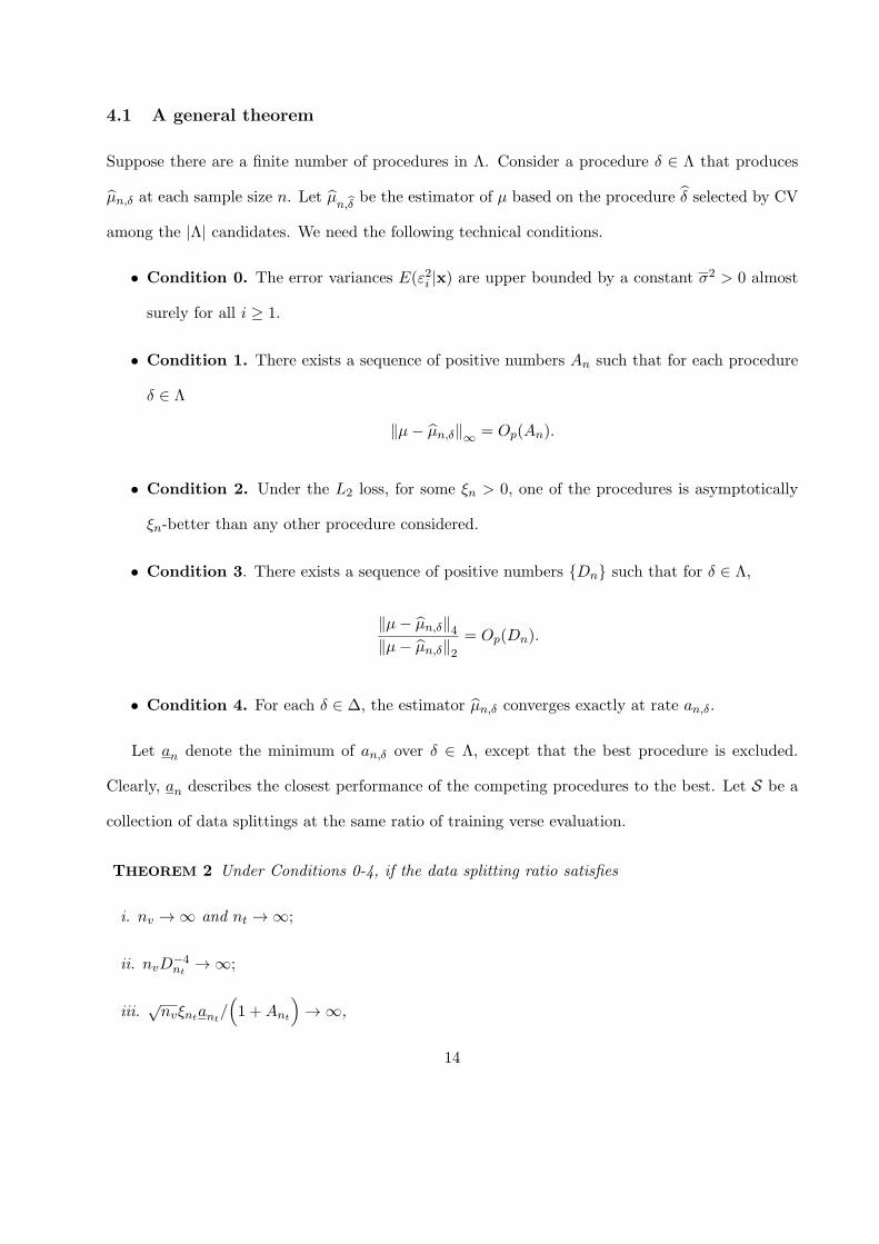
4.1 A general theorem

Suppose there are a finite number of procedures in Λ. Consider a procedure δ ∈ Λ that produces

µn,δ at each sample size n. Let µn,δ

be the estimator of µ based on the procedure δ selected by CV

among the |Λ| candidates. We need the following technical conditions.

• Condition 0. The error variances E(ε2i |x) are upper bounded by a constant σ2 > 0 almost

surely for all i ≥ 1.

• Condition 1. There exists a sequence of positive numbers An such that for each procedure

δ ∈ Λ

∥µ− µn,δ∥∞ = Op(An).

• Condition 2. Under the L2 loss, for some ξn > 0, one of the procedures is asymptotically

ξn-better than any other procedure considered.

• Condition 3. There exists a sequence of positive numbers {Dn} such that for δ ∈ Λ,

∥µ− µn,δ∥4∥µ− µn,δ∥2

= Op(Dn).

• Condition 4. For each δ ∈ ∆, the estimator µn,δ converges exactly at rate an,δ.

Let an denote the minimum of an,δ over δ ∈ Λ, except that the best procedure is excluded.

Clearly, an describes the closest performance of the competing procedures to the best. Let S be a

collection of data splittings at the same ratio of training verse evaluation.

THEOREM 2 Under Conditions 0-4, if the data splitting ratio satisfies

i. nv → ∞ and nt → ∞;

ii. nvD−4nt

→ ∞;

iii.√nvξntant

/(1 +Ant

)→ ∞,

14

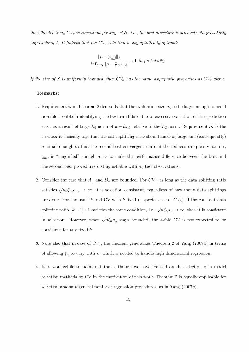
then the delete-nv CVv is consistent for any set S, i.e., the best procedure is selected with probability

approaching 1. It follows that the CVv selection is asymptotically optimal:

∥µ− µn,δ

∥2infδ∈Λ ∥µ− µn,δ∥2

→ 1 in probability.

If the size of S is uniformly bounded, then CVa has the same asymptotic properties as CVv above.

Remarks:

1. Requirement ii in Theorem 2 demands that the evaluation size nv to be large enough to avoid

possible trouble in identifying the best candidate due to excessive variation of the prediction

error as a result of large L4 norm of µ− µn,δ relative to the L2 norm. Requirement iii is the

essence: it basically says that the data splitting ratio should make nv large and (consequently)

nt small enough so that the second best convergence rate at the reduced sample size nt, i.e.,

ant, is “magnified” enough so as to make the performance difference between the best and

the second best procedures distinguishable with nv test observations.

2. Consider the case that An and Dn are bounded. For CVv, as long as the data splitting ratio

satisfies√nvξntant

→ ∞, it is selection consistent, regardless of how many data splittings

are done. For the usual k-fold CV with k fixed (a special case of CVa), if the constant data

splitting ratio (k− 1) : 1 satisfies the same condition, i.e.,√nξnan → ∞, then it is consistent

in selection. However, when√nξnan stays bounded, the k-fold CV is not expected to be

consistent for any fixed k.

3. Note also that in case of CVv, the theorem generalizes Theorem 2 of Yang (2007b) in terms

of allowing ξn to vary with n, which is needed to handle high-dimensional regression.

4. It is worthwhile to point out that although we have focused on the selection of a model

selection methods by CV in the motivation of this work, Theorem 2 is equally applicable for

selection among a general family of regression procedures, as in Yang (2007b).

15

5. The set of sufficient conditions on data splitting of CV in Theorem 2 for selection consistency

has not been shown to be necessary. We tend to think that when An and Dn are bounded and

ξn (taken as large as possible) properly reflects the relative performance of the best procedure

over the rest, the resulting requirement of nv → ∞, nt → ∞ and√nvξntant

→ ∞ may well

be necessary, possibly under additional minor conditions.

6. Conditions 1 and 3 are basically always satisfied. But what is important here is the orders

of magnitude of An and Dn, which affect the sufficient requirement on data splitting ratio to

guarantee the selection consistency.

4.2 A comparison of traditional and high-dimensional situations

In the high-dimensional regression case, the number of features pn is typically assumed to increase

with n and the true model size qn may also grow. We need to point out that Yang (2007b) deals with

the setting that the true regression function is fixed when there are more and more observations.

In the new high-dimensional regression setting, the true regression function may change with n.

The theorems in Yang (2007b) and in the present paper help us understand some key differences

in terms of proper use of CV between the two situations.

1. In the traditional case, the estimator based on the true model is asymptotically better than

that based on a model with extra parameters according to the definition in Yang (2007b). But

the definition does not work for the high-dimensional case, hence the new definition (Definition

1). Indeed, when directly comparing the true model of size qn → ∞ and a larger model with

∆qn extra terms, the estimator of the true model is asymptotically√

∆qn/qn-better than

the larger model. Clearly, if ∆qn is bounded, then the true model is not asymptotically

better under the definition in Yang (2007b). Based on the new sufficient result in this paper,

nv

(∆qnqn

)(qn+∆qn

nt

)→ ∞ is adequate for CV to work. There are different scenarios for the

sufficient data splitting conditions:

16

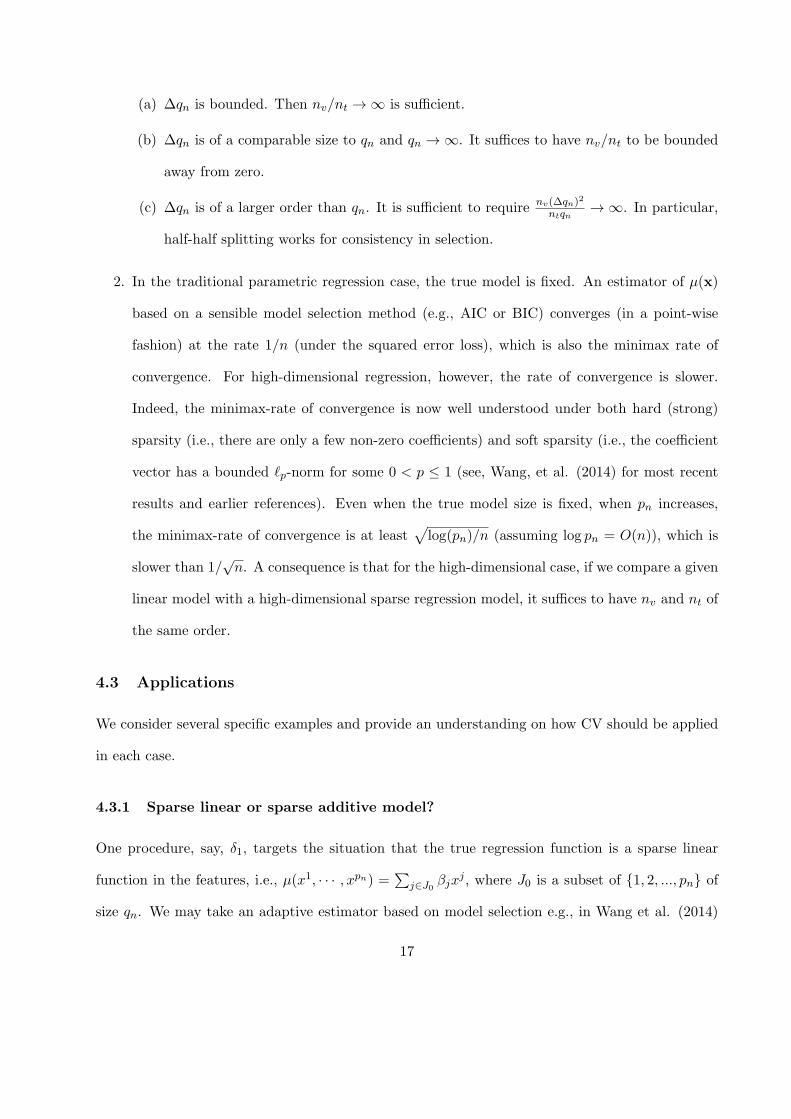
(a) ∆qn is bounded. Then nv/nt → ∞ is sufficient.

(b) ∆qn is of a comparable size to qn and qn → ∞. It suffices to have nv/nt to be bounded

away from zero.

(c) ∆qn is of a larger order than qn. It is sufficient to require nv(∆qn)2

ntqn→ ∞. In particular,

half-half splitting works for consistency in selection.

2. In the traditional parametric regression case, the true model is fixed. An estimator of µ(x)

based on a sensible model selection method (e.g., AIC or BIC) converges (in a point-wise

fashion) at the rate 1/n (under the squared error loss), which is also the minimax rate of

convergence. For high-dimensional regression, however, the rate of convergence is slower.

Indeed, the minimax-rate of convergence is now well understood under both hard (strong)

sparsity (i.e., there are only a few non-zero coefficients) and soft sparsity (i.e., the coefficient

vector has a bounded ℓp-norm for some 0 < p ≤ 1 (see, Wang, et al. (2014) for most recent

results and earlier references). Even when the true model size is fixed, when pn increases,

the minimax-rate of convergence is at least√

log(pn)/n (assuming log pn = O(n)), which is

slower than 1/√n. A consequence is that for the high-dimensional case, if we compare a given

linear model with a high-dimensional sparse regression model, it suffices to have nv and nt of

the same order.

4.3 Applications

We consider several specific examples and provide an understanding on how CV should be applied

in each case.

4.3.1 Sparse linear or sparse additive model?

One procedure, say, δ1, targets the situation that the true regression function is a sparse linear

function in the features, i.e., µ(x1, · · · , xpn) =∑

j∈J0 βjxj , where J0 is a subset of {1, 2, ..., pn} of

size qn. We may take an adaptive estimator based on model selection e.g., in Wang et al. (2014)

17

that automatically achieves the minimax optimal rate qn(1 + log(pn/qn))/n ∧ 1 without knowing

qn.

The other procedure, say, δ2, is based on a sparse nonparametric additive model assumption,

i.e., µ(x1, · · · , xpn) =∑

j∈J1 βjψj(xj), where J1 is a subset of {1, 2, ..., pn} of size dn and ψj(x

j) is

a univariate function in a class with L2 metric entropy of order (ϵ)−1/α for some α > 0. Raskutti

et al. (2012) construct an estimator based on model selection that achieves the rate

(dn(1 + log(pn/dn))/n+ dnn

− 2α2α+1

)∧ 1,

which is also shown to be minimax rate optimal.

Under the sparse linear model assumption, δ2 is conjectured to typically still converge at the

above displayed rate and is suboptimal. When the linear assumption fails but the additive model

assumption holds, δ1 does not converge at all. Since we do not know which assumption is true, we

need to choose between δ1 and δ2.

From Theorem 2, if pn → ∞, it suffices to have both nt and nv of order n. Thus any fixed data

splitting ratio, e.g., half-half, works fine theoretically. Note also that the story is similar when the

additive model is replaced by a single index model, for instance.

4.3.2 A classical parametric model or a high-dimensional exploratory model?

Suppose that an economic theory suggests a parametric regression model on the response that

depends on a few known covariates. With availability of big data and high computing power, many

possibly relevant covariates can be considered for prediction purpose. High-dimensional model

selection methods can be used to search for a sparse linear model as an alternative. The question

then is: Which one is better for prediction?

In this case, when the parametric model holds, the estimator converges at the parametric rate

with L2 loss of order 1/√n, but the high-dimensional estimator converges more slowly typically at

18

least by a factor of√log pn. In contrast, if the parametric model fails to take advantage of useful

information in other covariates but the sparse linear model holds, the parametric estimator does

not converge to the true regression function while the high-dimensional alternative does.

In this case, from Theorem 2, it suffices to have nv at order larger than n/ log(pn). In particular,

with pn → ∞, half-half splitting works.

4.3.3 Selecting a model on a solution path

Consider a path generating method that asymptotically contains the true model of size qn on the

path of sequentially nested models. To select a model on the path obtained based on separate data,

we use CV. From Section 4.2, with a finite solution path, nv/nt → ∞ guarantees against overfitting.

As for under-fitting, assuming that the true features are nearly orthonormal, a missing coefficient β

causes squared bias of order β2. To make the true model have a better estimator than that from a

sub-model, it suffices to require β to be at least a larger enough multiple of√log(pn)/n. Then with

probability going to 1, the choice of nv/nt → ∞ is enough to prevent under-fitting. Consequently,

the true model can be consistently selected.

5 Simulations

In the simulations below, we primarily study the selection, via cross-validation, among modeling

procedures that include both model selection and parameter estimation. Since CV with averaging

is much more widely used in practice than CV with voting and they exhibit similar performance

(sometimes slightly better for CVa) in out experiments, all results presented in Sections 5, 6 and

7 are of CV with averaging. In each replication |S| = S = 400 random splittings are performed to

calculate average CV errors.

The design matrix X = (Xi,j) (i = 1, · · · , n; j = 1, · · · , pn) is n × pn and each row of X is

generated from the multivariate normal distribution with mean 0 and an AR(1) covariance matrix

with marginal variance 1 and autocorrelation coefficient ρ, independently. Two values of ρ, −0.5

19

and 0.5 are examined. The responses are generated from the model

Yi =

pn∑j=1

βjXi,j + εi (11)

where ε′is (i = 1, · · · , n) are iid N(0, 1) and β = (β1, .., βpn)T is a pn-dimensional vector including

qn nonzero coefficients and (pn − qn) zeros.

5.1 The performance of CV at different levels of splitting ratio

In this subsection the performances of CV at different splitting ratios are investigated in both

parametric and (practically) nonparametric settings. Let n = 1000 and pn = 20. Three information

criteria AIC, BIC and BICc (λ = log n + log log n) are considered. Our goal here is not to be

comprehensive. Instead, we try to capture archetype behaviors of the CV’s (at different splitting

ratios) under parametric and nonparametric settings, which offer insight on this matter. In each

simulating study, 1000 replications are performed.

The cross-validation error is calculated in two steps. Firstly, the training set including nt

sample points is generated by random subsampling without replacement and the remaining nv

observations are put into the validation set Iv. We define τ = nv/n as the validating proportion.

Twenty validating proportions equally spaced between (pn + 5)/n and (n − 5)/n are tested. In

the second step, a modeling procedure δ is selected and fitted by the training set from the three

candidates AIC, BIC and BICc, and the validating error is calculated.

The above two steps are repeated 400 times through random subsampling and their average

for each criterion is its final CV error (6). The criterion attaining the minimal final CV error is

selected.

In the two contrasting scenarios, the effects of τ on i) the distribution of the difference of the CV

errors of any two competitors; ii) the probability of selecting the better criterion; iii) the resulting

estimation efficiency: for each pair of criteria, the smaller MSE of the two over that based on the CV

20

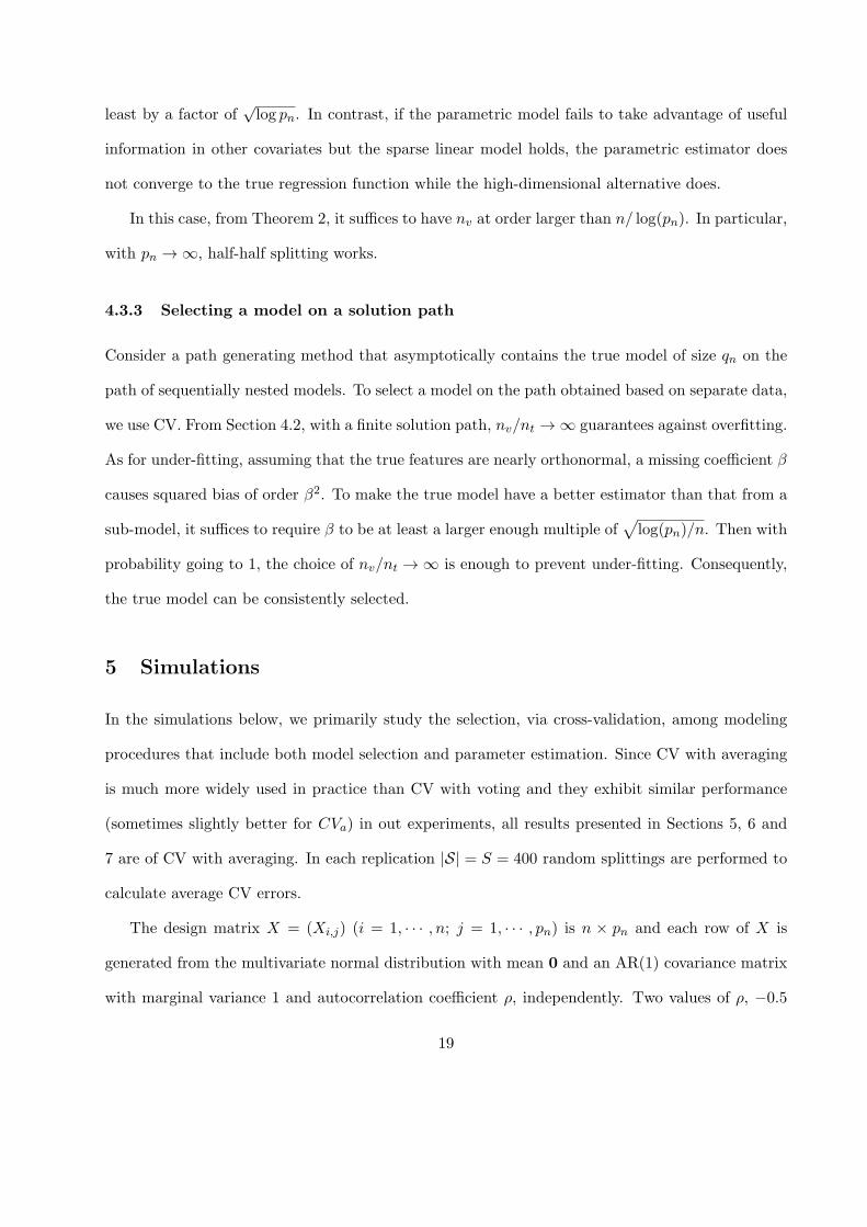
selection are presented in Figures 1 and 2, displayed on the first three rows (the individual values

over the 1000 replications, mean and standard deviation), the 4th row and 5th row, respectively.

5.1.1 The parametric scenario

Here we take (β1, β2) = (2, 2) and βj = 0 (3 ≤ j ≤ 20), and BICc beats the other two criteria in

terms of predictive accuracy measured by mean squared error.

Figure 1 about here.

From the plots of AIC v.s. BIC and AIC v.s. BICc of Figure 1, the performance of CV in terms

of proportion of identifying the better procedure (i.e., the larger λn in this case) and the comparative

efficiency experience a two-phase process: improve and then stay flat when the validating proportion

τ goes up from 0 to 1. As τ is above 50%, the proportion of selecting the better procedure by CV

is close to 1. In the plot BIC v.s. BICc, the proportion of selecting the better procedure and the

comparative efficiency increase slightly from 95% to 1 across different levels of splitting ratios due

to the smaller difference between the two penalty coefficients in contrast to the other two pairs.

Another observation is that the mean of the CV error difference experiences a two-phase process,

a slight increase as the validating proportion τ is less than 90% followed by a sharp increase as τ

goes above 90%. The standard deviation of CV error difference experiences a three-phase process,

sharp decrease, slight decrease and jump-up. The data splitting ratio plays a key role here: the

increase of validating size smoothes out the fluctuations of the CV errors, but when the training

size is below some threshold, the parameter estimation errors become quite wild and cause trouble

in terms of the ranking of the candidate modeling procedures.

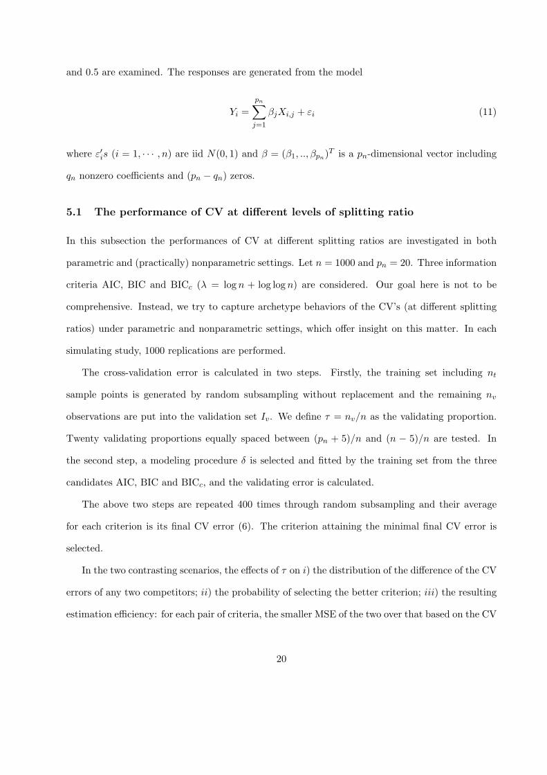
5.1.2 The nonparametric scenario

Now we take βj = 1/j (j = 1, · · · , 20), where, with pn fixed at 20 and n not very large (e.g., around

1000), AIC tends to outperform the other two criteria. This is a “practically nonparametric”

situation (see Liu and Yang, 2011).

21

Figure 2 about here.

As indicated by Figure 2, the performance of CV in terms of the probability of selecting the

better procedure (i.e., the smaller λn here) exhibits different patterns than the parametric scenario.

Though the sample standard deviation of CV error difference exhibits similar patterns, the mean of

CV error difference between two procedures increases from a negative value (which is the good sign

to have here) to a positive value, whereas in the parametric scenario the sign does not change. In

nonparametric frameworks, as the validating proportion τ is above 80% the best model at the full

sample size n suffers from low sample size more than the underfitting model due to large parameter

estimation error. As a result, the comparative efficiency and the proportion of selecting the better

procedure experiences a three-phase process, improvement, steadiness and deterioration as τ runs

across 10% and 90%.

In summary of the illustration, the half-half splitting CV with S = 400 splittings selected the

better procedures with almost 100 percent chance between any two competitors considered here in

both data generating scenarios. This is certainly not expected to be true always, but our experience

is that the half-half splitting usually works quite well.

5.2 Combine different procedures by delete-n/2 CV in random design regression

In this section we look into the performance of delete-n/2 CV with S = 400 splittings to combine

the power of various procedures in traditional and high dimensional regression settings. As a

comparison we examine the performances of delete-0.2n, delete-0.8n and 10-fold CV as well. In

each setting, 500 replications are performed.

The final accuracy of each regression procedure is measured in terms of the L2 loss, which is

calculated as follows. Apply a candidate procedure δ to the whole sample and use the selected

model Mδ to estimate the mean function at 10,000 sets of independently generated features from

the same distribution. Denote the estimates and the corresponding true means by Y Pi (Mδ) and µ

′i

22

(i = 1, · · · , 10000) respectively. The squared loss then is

Loss(δ) =1

10000

10000∑i=1

(µ′i − Y P

i (Mδ))2, (12)

which simulates the squared L2 loss of the regression estimate by the procedure. The square loss

of any version of CV is the square loss of the final estimator when using CV for choosing among

the model selection methods. The risks of the competing methods are the respective average losses

of the 500 replications.

5.2.1 Combine AIC, BIC and BICc by delete-n/2 CV

In this subsection we compare the predictive performances of AIC, BIC and BICc with different

versions of CV’s in terms of the average of squared L2 loss in (12). The data are generated by

Yi =

15∑j=1

βjXi,j + εi; where βj = 0.25/j (1 ≤ j ≤ 10); βj = 0 (11 ≤ j ≤ 15), (13)

whereXi,j and εi are simulated by the same method as before. Three different sample sizes n = 100,

10,000 and 500,000 are considered.

Table 1 about here.

As shown by Table 1, when the sample size is small or extremely large, BICc outperforms

the other two competitors (at n = 100) or performs the best (tied with BIC) (at n = 500, 000)

and delete-n/2 and delete-0.8n CV’s have similar performance to BICc, whereas for moderately

large sample size (n=10,000) AIC dominates others and delete-n/2 CV shares similar performance

with AIC. In summary, over the three model selection criteria, CV equipped with half-half splitting

impressively achieves adaptivity in hiring the unknown “top gun” to various settings of sample size,

signal-to-noise ratio and design matrix structure (some results are not presented here). Other types

of CV perform generally worse than the delete-n/2 CV. Although the true model is parametric (but

23

practically nonparametric at n = 10, 000), based on the results in Liu and Yang (2011), it is not

surprising at all to see the relative performance between AIC and BIC switches direction twice,

with BIC having the last laugh.

5.2.2 Combine SCAD, MCP, LASSO and stepwise regression by delete-n/2 CV

In this subsection we compare the predictive performances, in terms of the average squared L2 loss

in (12), of SCAD (Fan and Li, 2001), MCP (Zhang, 2010), LASSO (Tibshirani, 1996), Stepwise

regression plus RIC (Foster and George, 1994), that is, λn = 2 log pn in (8) (STRIC), against the

delete-n/2 CV used to choose one of them with S = 400 splittings (some other versions of CV are

included as well for comparison). The data are generated by

Yi =

pn∑j=1

βjXi,j + εi; βj = 6/j (1 ≤ j ≤ qn), βj = 0 (qn + 1 ≤ j ≤ pn) (14)

where Xi,j and εi are simulated by the same method as before. We examine three different qn

values, qn = 1, 5 and 10 with n = pn = 500.

Table 2 about here.

As shown by Table 2 when qn = 1, ρ = ±0.5 and qn = 5, ρ = −0.5, SCAD and MCP outperform

the other two competitors, which tend to include some redundant variables, and delete-n/2 and

delete-0.8n CV’s have similar performance to SCAD and MCP while delete-0.2n and 10-fold CV’s

fail to select the best procedure. When qn = 10, ρ = ±0.5, STRIC dominates the others, and

SCAD and MCP tend to exclude some relevant variables. The delete-n/2, delete-0.2n and 10-fold

CV’s perform similarly to STRIC, whereas delete-0.8n CV performs poorly.

It is worth noting that when qn = 5 and ρ = 0.5, delete-n/2 CV outperforms all four original

candidate procedures (SCAD, MCP, LASSO and STRIC) significantly by making a “smart selec-

tion”. Examining the output of the 500 replications we found that the data, which are generated

randomly and independently in each replication, exhibit a parametric pattern in some cases such

24

that MCP performs best, and a nonparametric pattern in other cases such that STRIC shows

great advantages. Overall, delete-n/2 CV picks up the best procedure adaptively and on average it

achieves lower loss than the best one of all the four candidates. This “smart selection” phenomenon

will also be observed in Section 6.

In summary, half-half splitting CV outperforms other types of CV in terms of procedure selec-

tion, which typically includes two steps: model selection and parameter estimation. Moreover, the

simulations confirm the theoretical results in Section 3 and 4 and provides a guidance in splitting

ratio choice, i.e., half-half splitting tends to work very well for the selection of optimal procedures

across various settings. In general high-dimensional cases, the different model selection criteria may

have drastically different performances, as seen in the present example, and a consistent choice of

the best among them, as done by half-half splitting CV is a practically important approach to move

beyond sticking to one’s favorite criterion or choosing one arbitrarily.

6 A Real Data Example

Physical constraints on the production and transmission of electricity make it the most volatile

commodity. For example, in the city of New York, the price at peak hours of a hot and humid

summer day can be hundred times the lowest level. Therefore, financial risk management is often

a high priority for participants in deregulated electricity markets due to the substantial price risks.

The cost of supplying the next megawatt of electricity determines its price in the wholesale

market. Take the regional power market of New York as an example, it has roughly four hundred

locations (i.e., nodes) with different prices due to local supply and demand. When two close nodes

are connected by a high-voltage transmission line, they tend to share similar prices because of the

low transmission cost between them. Power market participants face unique risks from the price

volatility. So modeling prices across nodes is essential to prediction and risk hedging. The data

we have here cover 423 nodes (pn = 423) and 422 price observations per node (n = 422). In the

absence of additional information (such as distance between nodes and their connectivity), the goal

25

here is to estimate one node by the rest via linear modeling (the unit of the response is dollar

per megawatts). This is a high dimensional linear regression problem that makes adaptive model

selection challenging. In fact, we will show next that different selection criteria picked very different

models.

We compare delete-n/2 CV with MCP, SCAD, LASSO, and STRIC with respect to predictive

performances in three steps. Firstly, the 422 observations are randomly divided into an estimation

set and a final evaluation set according to two pre-defined ratios, 75:25 and 25:75. Four models are

chosen by MCP, SCAD, LASSO and STRIC, respectively, from the estimation set and then used

to make predictions on the evaluation set. Secondly, a procedure is selected by delete-n/2 CV from

these four candidate procedures, where the delete-n/2 CV is implemented by evenly splitting the

estimation set into a training part and a validation part in 400 subsampling rounds (i.e., S = 400).

A model is thus developed by the delete-n/2 CV procedure from the estimation set and then used

to make predictions on the final evaluation set. The prediction error is the average of squared L2

loss at each node in the final evaluation set. Finally, repeat the above two steps 100 times for

the two ratios 75:25 and 25:75 and the average of square root of prediction errors based on 500

replications is displayed in the following table for each of the five procedures. The “permutation

standard error” (which is not really a valid standard error of the CV error due to dependence of

the permutations) is shown in the parentheses respectively.

Table 3 about here.

When the estimation set is small (25:75), SCAD and MCP exhibit much larger “permutation

standard errors” because the high correlations among the features (nodes) and small estimation

sample size caused a few large prediction errors in the 500 replications for the two methods, while

LASSO was more stable. Overall, the delete-n/2 CV procedure yields the best predictive accuracy.

26

7 Misconceptions on the use of CV

Much effort has been made on proper use of CV (see, e.g., Hastie et al, 2009, Chapter 7.10; Arlot

and Celisse, 2010 for a comprehensive review). Unfortunately, some influential work in the literature

that examines CV methods, while making important points, does not clearly distinguish different

goals and thus draws inappropriate conclusions. For instance, regarding which k-fold CV to use,

Kohavi (1995) focused only on accuracy estimation in all the numerical work, but the observations

there (which will be discussed later) are often directly passed onto model selection. The work

has been very well-known and the recommendation there that the best method to use for model

selection is 10-fold CV has been followed by many in computer science, statistics and other fields.

In another direction, we have seen publications that use LOO CV on real data to rank parametric

and nonparametric methods.

Applying CV without factoring in the objective can be a very serious mistake. There are three

main goals in the use of CV. The first is for estimating the prediction performance of a model or a

modeling procedure. The second and third goals are often both under the same name of “CV for

model selection”. However, there are different objectives of model selection, one as an internal step

in the process of producing the final estimator, the other as for identifying the best candidate model

or modeling procedure. With this distinction spelled out, the second use of CV is to choose a tuning

parameter of a procedure or a model/modeling procedure among a number of possibilities with the

end goal of producing the best estimator (see e.g., van der Vaart et al. (2006) for estimation bounds

in this direction). The third use of CV is to figure out which model/modeling procedure works the

best for the data.

The second and third goals are closely related. Indeed, the third use of CV may be applied for

the second goal, i.e., the declared best model/modeling procedure can be then used for estimation.

Note that this type of application, with a proper data splitting ratio, results in asymptotically

optimal performance in estimation, as shown in Sections 3 and 4 in the present paper. A caveat is

that this asymptotic optimality may not always be satisfactory. For instance, when selecting among

27

parametric models in a “practically non-parametric” situation with the fixed true model being one

of the candidates, a model selection method built for the third goal (such as BIC) may perform

very poorly for the second goal (see, e.g, Shao, 1997; Liu and Yang, 2011).

In the reverse direction, the best CV for the second goal does not necessarily imply the achieve-

ment of the third goal. For instance, in the nonparametric regression case, the LOO CV is asymp-

totically optimal for selecting the order of nested models (e.g., Li, 1987), but it is not true that

the selected model agrees with the best choice with probability going to 1. Indeed, to achieve the

asymptotic optimality in estimation, one does not have to be able to identify the best candidate.

As seen in Section 4, in high-dimensional linear regression with the true model dimension qn → ∞,

an overfitting model with a bounded number of extra terms performs asymptotically as well as

the true model. Furthermore, identifying the best choice with probability going to 1 may lead to

sub-optimal estimation of the regression function in a minimax sense (Yang, 2005).

The following misconceptions are frequently seen in the literature, even up to now.

7.1 “Leave-one-out (LOO) CV has smaller bias but larger variance than leave-

more-out CV”

This view is quite popular. For instance, Kohavi (1995, Section 1) states: “For example, leave-one-

out is almost unbiased, but it has high variance, leading to unreliable estimates”.

The statement, however, is not generally true. In fact, in least squares linear regression, Burman

(1989) shows that among the k-fold CVs, in estimating the prediction error, LOO (i.e., n-fold CV)

has the smallest asymptotic bias and variance. For k < n, if all possible removals of n/k observations

are considered (instead of a single k-fold CV), is the error estimation variance then smaller than

that from LOO? The answer is No. As an illustration, consider the simplest regression model:

Yi = θ + εi, where θ is the only mean parameter and εi are iid N(0, σ2) with σ > 0. Then a

theoretical calculation (Lu, 2007) shows that LOO has the smallest bias and variance at the same

time among all delete-nv CVs with all possible nv deletions considered.

28

A simulation is done to gain a numerical understanding. The data are generated by (11) with

n = 50, pn = 10, qn = 4, σ = 4 and β1 = · · · = β4 = 2 and βj = 0 (5 ≤ j ≤ 10), and the design

matrix is generated the same way as in Section 5.1 but with ρ = 0. The delete-nv (nv = 1, 2 and

5) CV’s are compared through 10,000 independent replications. Three cases are considered: CV

estimate of the prediction error for the true model (with the parameters estimated), for the model

selection of AIC over all subset models, and for the model selection by BIC. In each replication, the

CV error estimate is the average of all(nnv

)splittings as nv = 1 and 2, and of 1000 subsamplings as

nv = 5. The theoretical mean prediction error at the sample size (n = 50), as well as the bias and

variance of the CV estimator of the true mean prediction error in each case are simulated based

on the 10,000 runs. The standard errors (in the parentheses) for each procedure are also reported

(the delta method is used for the standard error of the variance estimate).

As a comparison, we report the average of permutation variance, which refers to the sample

variance of the CV errors over different data splittings in each data generation of 50 observations.

It is worth pointing out that the permutation variance is sometimes mistaken as a proper estimate

of the variance of the CV error estimate. We also present the average pairwise differences of bias

and variance with standard errors between delete-1 and delete-2 given to make it clear that the

statistical significance on the differences is obvious.

Table 4 about here

As revealed by the above table, as expected, the bias of delete-nv CV errors is increasing in nv

in all cases. The variance exhibits more complex patterns: for the true model, LOO in fact has

the smallest variability; but for the AIC procedure, the variance decreases in nv (for nv ≤ 5); in

the case of BIC, the variance first decreases and then increases as nv goes up from 1 to 5. In the

example, LOO still has smaller MSE for the AIC procedure compared to the delete-5 CV.

Note that the permutation variance, which is not what one should care about regarding the

choice of a CV method, consistently has the pattern of decreasing in nv. This deceptive mono-

29

tonicity may well be a contributor to the afore-stated misconception. See Arlot and Celisse (2010,

Section 5) for papers that link instability of modeling procedures to the CV variability.

7.2 “Better estimation (e.g., in bias and variance) of the prediction error by

CV means better model selection”

This seemingly obviously correct statement is actually false! To put the issue in a slightly different

setup, suppose that a specific data splitting ratio (nt : nv, with nt+nv = n) works very well to tell

apart correctly two competing models. Now suppose we are given another n iid observations from

the same population. If we put all the new n observations into estimation (i.e., with training size

now n+ nt) and use the same amount of observations (i.e., nv) as before for validation. With the

obviously improved estimation capability and unchanged validation capability, we should do better

in comparing the two models, right? Wrong! This is the cross validation paradox (Yang, 2006).

The reason is that prediction error estimation and comparing models/procedures are drastically

different targets. For the latter, when comparing two models/procedures that are close to each

other, the improved estimation capability by having more observations in the estimation part only

makes the models/procedures more difficult to be distinguished. The phenomenon that nv needs to

be close to n for consistent model selection in linear regression was first discovered by Shao (1993).

In the context of comparing two procedures (e.g., a parametric estimator and a kernel estimator),

this high demand on nv may not be necessary, as shown in Yang (2006, 2007b). The present

work provides a more general result suitable for both traditional and high-dimensional regression

settings.

In the above, we focused on the third goal of using CV. It is also useful to note that better

estimation of the prediction error does not mean better model selection in terms of the second goal

of using CV either (see Section 5 of Breiman and Spector, 1992).

30

7.3 “The best method to use for model selection is 10-fold CV”

As mentioned earlier, Kohavi (1995) endorsed the 10-fold CV as the best for model selection on the

ground that it may often attain the smallest variance and the mean squared error in the estimation

of prediction errors. Based on the previous subsection, the subsequent recommendation of 10-

fold CV for model selection in that paper does not seem to be justified. Indeed, from Tables 1

and 2, it is seen that the 10-fold CV performs worse than the delete-n/2 CV for estimating the

regression function (repeated 10-fold does not help much here). Based on our theoretical results

and our experience, it is expected that for selection consistency purpose, delete-n/2 CV usually

works better than 10-fold CV. The adaptively higher probability of selecting the best candidate by

the delete-n/2 CV usually (but not always) implies better estimation.

Now we examine the performance of the 10-fold CV relative to other versions of CV in terms of

prediction error estimation. Some simulations are run in the same setting as the above subsection

except n = 100 and pn = 10 or 1000 (for the LASSO, SCAD and MCP cases). Since the bias aspect

is clear in ranking, we focus on the variance and the MSE. The outputs are as follows.

Figures 3 and 4 about here

The simulations demonstrate that LOO possesses the smallest variance for a fixed model, which

can be the true model, an underfitting or overfitting model. However, if model selection is involved,

the performance of LOO worsens in variability as the model selection uncertainty gets higher due

to large model space, small penalty coefficients and/or the use of data-driven penalty coefficients.

It can lose to the 10-fold CV, which indeed can sometimes (e.g., AIC case) achieve the smallest

variance and MSE as observed by Kohavi (1995).

The highly unstable cases of LASSO, SCAD and MCP are interesting. As k decreases, we

actually see that the variance drops monotonically for each of them (except the k-fold version,

which gives misleading representation). However, the bias increases severely for small k, making

the MSE increasing rapidly from k = 10 down to 2. The MSE is minimal for the LOO in all cases

31

except AIC (and BIC with repeated k-fold), which supports that the statement of the title of this

subsection is a misconception.

Since a single k-fold CV without repetition often exhibits large variability as seen above, we

examine the performance of repeated k-fold CVs as it is repeated 200 times with random data

permutations. The results are summarized in Figure 5.

Figure 5 about here

Figure 5 clearly shows that the variance of repeated k-fold CVs drops sharply for small k as the

number of repetitions increases up to 10-20 and decreases only slightly afterwards. In other words,

repeated k-fold CVs achieve much improvement on prediction error estimation over single k-fold

CVs at the cost of only a limited number of repetitions, especially for small k.

Furthermore, S repetitions of delete-n/k and S/k repetitions of k-fold CV (S = 100 for LASSO,

SCAD and MCP and S = 500 for other methods) are compared and presented in Figure 3. It

shows that the repeated k-fold CVs outperforms delete-n/k CV at roughly the same amount of

computations.

Based on the above, we generally suggest repeated k-fold CVs (obviously except k = n) as a

more efficient/reliable alternative to delete nv (n/nv = k) or single k-fold CVs regardless of the

modeling procedures if the primary goal is prediction error estimation. As for the choice of k in

repeated k-fold, it seems a large k (e.g., LOO) is preferred. LOO is a safe choice: even if it is not

the best, it does not lose by much to other CVs for the prediction error estimation.

In the above simulations, uncorrelated features (ρ = 0) are assumed. We also examined the

outputs by setting ρ = 0.5 and −0.5, and the major findings are pretty much the same.

32

8 Concluding remarks

8.1 Is the 2nd level CV really necessary?

In the introduction, in the context of dealing with parametric regression models as candidates,

two questions were raised regarding the legitimacy of our use of CV for selecting a model selection

criterion. The first question is that for achieving asymptotic optimality of AIC and BIC adaptively,

why not consider GIC, which contains AIC and BIC as special cases. The fact of matter is that

one does not know which penalty constant λn to use and for any determinist sequence of λn, it is

easy to see that you can only have at most one of the properties of AIC and BIC, but not both.

Therefore for adaptive model selection based on GIC, one must choose λn in a data driven fashion.

Our approach is in fact one way to proceed: it chooses between the AIC penalty sequence λn = 2

and the BIC penalty λn = log n, and we have shown that this leads to an asymptotic optimality

for both the AIC and BIC worlds at the same time.

The other question asks why not use CV to select a model among all those in the list instead of

the two by AIC and BIC. Actually, it is well-known that CV on the original models behaves some-

where between AIC and BIC, depending on the data splitting ratio (e.g., Shao, 1997). Therefore it

in fact cannot offer adaptive asymptotic optimality as we were seeking. More specifically, if one uses

CV to find the best model in the parametric scenario, then one must have nv/n → 1. However, if

the true regression function is actually infinite-dimensional, such a choice of CV results in selecting

a model of size of a smaller order than the optimal, leading to sub-optimal rate of convergence.

Conversely, for the infinite-dimensional case, LOO CV typically performs optimally, but should

the true regression function be among the candidate models, it fails to be optimal. So any use of

CV on the candidate models in fact cannot enjoy optimal performance under both parametric and

nonparametric assumptions. The second level use of CV, i.e., CV on the AIC and BIC, comes to

the rescue, as we have shown. This demonstrates the importance of second level of model selection,

i.e., the selection of a model selection criterion. With the general applicability, CV has a unique

33

advantage to do the second level procedure selection. Clearly, CV is also applicable for comparing

modeling procedures that are not based on parametric models.

Therefore, we can conclude that the use of CV on modeling procedures can be a powerful tool

for adaptive estimation that suits multiple scenarios simultaneously. In high-dimensional settings,

the advantage of this approach can be even more remarkable. Indeed, with exponentially many or

more models being considered, any practically feasible model selection method constructed is good

typically for one or a few specific scenarios, and CV can be used to choose among a number of

methods in hope that the best one handles the true data generation process well.

Our results reveal that for selection consistency, the choice of splitting ratio for CV needs to

balance two ends, the ability to order the candidates in terms of estimation accuracy based on

the validation part of data (which favors large validation size) and the need to have the same

performance ordering at the reduced sample size as at the full sample size (which can go wrong

when the size of the estimation part of data is too low). Overall, unless one is selecting among

parametric models at least one of which captures the statistical behavior of the data generating

process very well, we recommend half-half splitting or slightly more observations for evaluation

when applying CV for the goal of identifying the best modeling procedure.

8.2 Summary and discussion

In the literature, even including recent publications, there are overly taken recommendations. The

general suggestion of Kohavi (1995) to use 10-fold CV has been widely accepted. For instance,

Krstajic et al (2014, page 11) state: “Kohavi [6] and Hastie et al [4] empirically show that V-fold

cross-validation compared to leave-one-out cross-validation has lower variance”. They consequently

take the recommendation of 10-fold CV (with repetition) for all their numerical investigations. In

our view, such a practice may be misleading. First, there should not be any general recommendation

that does not take into account of the goal of the use of CV. In particular, examination of bias and

variance of CV accuracy estimation of a candidate model/modeling procedure can be a very different

34

matter from optimal model selection (with either of the two goals of model selection stated earlier).

Second, even limited to the accuracy estimation context, the statement is not generally correct. For

models/modeling procedures with low instability, LOO often has the smallest variability. We have

also demonstrated that for highly unstable procedures (e.g., LASSO with pn much larger than n),

the 10-fold or 5-fold CVs, while reducing variability, can have significantly larger MSE than LOO

due to even worse bias increase.

Overall, from Figures 3-4, LOO and repeated 50- and 20-fold CVs are the best here, 10-fold

is significantly worse, and k ≤ 5 is clearly poor. For predictive performance estimation, we tend

to believe that LOO is typically the best or among the best for a fixed model or a very stable

modeling procedure (such as BIC in our context) in both bias and variance, or quite close to the

best in MSE for a more unstable procedure (such as AIC or even LASSO with pn ≫ n). While

10-fold CV (with repetitions) certainly can be the best sometimes, but more frequently, it is in an

awkward position: it is riskier than LOO (due to the bias problem) for prediction error estimation

and it is usually worse than delete-n/2 CV for identifying the best candidate.

Not surprisingly, k-fold CV is an efficient way to use the data when compared to randomly

remove n/k observations k times. However, the k-fold CV is known to be often unstable. We agree

with Krstajic et al (2014) that given k, the repeated k-fold CV (even repeating just 10 or 20 times)

seems most promising for prediction error estimation.

In this work, we have considered both the averaging- and voting-based CVs, i.e, CVa and CVv.

Our numerical comparisons of the two tend to suggest that with the number of data splittings

suitably large, they perform very similarly, with CVa slightly better occasionally in risk of estimating

the regression function.

It is clear that the best CV depends on the goal of the usage and even with the same objective,

it may require different data splitting ratios in accordance with the nature of the target regression

function, the noise level, the sample size and the candidate estimators. Thus efforts should be put

on the understanding of the best version of CV for different scenarios, as we have done in this work

35

for the specific problem of consistent selection of a candidate modeling procedure. We have focused

on the squared L2 loss under homoscedastic errors. It remains to be seen how other choices of loss

and heteroscedasticity affect the performance of CV.

For consistently identifying the best candidate model and modeling procedure by CV, the

evaluation part has to be sufficiently large, the larger the better as long as the ranking of the

candidates in terms of risk at the reduced sample size of the training part stays the same as that

under the full sample size (which demands the training sample size to be not too small). The benefits

of having a large portion for evaluation are two-fold: 1) more observations for evaluation provide

better capability to distinguish the close competitors; 2) the fewer observations in the training part

make the accuracy difference between the close competitors magnified and the difference becomes

easier to detect even with the same amount of evaluation data.

With more and more model selection methods being proposed especially for high-dimensional

data, we advocate the use of cross-validation to choose the best for understanding/interpretation

or efficient prediction.

Acknowledgments

We thank two anonymous referees, the Associate Editor and the Editor, Dr. Yacine Ait-Sahalia,

for providing us with very insightful comments and valuable suggestions to improve the paper. The

research of Yuhong Yang was partially supported by the NSF Grant DMS-1106576.

Appendix: Proofs

Proof of Theorem 1 and Corollary 3.1:

We apply Theorem 2 to prove the results (note that the parts for CVv in Theorem 1 and Corollary

3.1 can be proved by applying Theorem 2 of Yang (2007b) directly with ξn = 1). The main task is

to verify the conditions required for that theorem, which is done below. Note that since the true

regression function is fixed, ξn can be taken to be just 1.

36

We first show that Condition 2 holds. Note that by Assumption 1, when the true model is not

in the list of the candidate models, µn,BIC is worse than µn,AIC . We next show that under the

given conditions, when the true model is among the candidates, µn,AIC is worse than µn,BIC .

Suppose the true model is m∗ and it is among the candidates. Then P (mn,BIC = m∗) → 1

as n → ∞ by Assumption 1. Note that L2(µ, µn,m∗) =∑m∗

j=0(αj − αj)2 and L2(µ, µn,AIC) =∑mn

j=0(αj − αj)2 + Emn

, where mn equals mn,AIC when AIC and BIC select different models and

equals mn,AIC + 1 otherwise. From above, with probability going to 1, we have L2(µ, µn,AIC) =∑mnj=0(αj −αj)

2 ≥∑m∗+1

j=0 (αj −αj)2, and L2(µ, µn,BIC) =

∑m∗

j=0(αj −αj)2 (again with probability

going to 1). Recall that αj =1n

∑ni=1 Yiφj(Xi). By the central limit theorem, for a given j ≥ m∗+1,

√nαj asymptotically has a non-degenerate normal distribution with mean zero and thus is bounded

away from zero in probability. Consequently n(αm∗+1)2 is bounded away from 0 in probability.

Together with that L2(µ, µn,BIC) converges to zero at order 1/n in probability and that

L2(µ, µn,AIC)

L2(µ, µn,BIC)≥ 1 +

n(αm∗+1)2

nL2(µ, µn,BIC),

it follows that µn,BIC is asymptotically better than µn,AIC according to Definition 1 with ξn = 1

(or Definition 1 of Yang, 2007b).

Now we show Condition 3 is satisfied, i.e., the ratio ∥µ − µn∥4/∥µ − µn∥2 is properly bound-

ed. Consider the model mn. For µn,mn , we have ∥µ − µn,mn∥44 =∫ 10

(∑mnj=0

(αj − αj

)φj(x) −∑∞

j=mn+1 αjφj(x))4dx ≤ 8

( ∫ 10

(∑mnj=0(αj − αj)φj(x)

)4dx+

∫ 10

(∑∞j=mn+1 αjφj(x)

)4dx

). Now

mn∑j=0

(αj − αj)φj(x) =1

n

n∑i=1

( mn∑j=0

µ(Xi)φj(Xi)φj(x)− αjφj(x))+

1

n

n∑i=1

( mn∑j=0

εiφj(Xi)φj(x)).

Consequently,

E

∫ 1

0

( mn∑j=0

(αj − αj)φj(x))4

dx =

∫ 1

0

E( mn∑

j=0

(αj − αj)φj(x))4

dx

≤ 8(∫ 1

0

E( 1n

n∑i=1

(

mn∑j=0

µ(Xi)φj(Xi)φj(x)− αjφj(x)))4dx+

∫ 1

0

E( 1n

n∑i=1

(

mn∑j=0

εiφj(Xi)φj(x)))4dx

).

37

Applying Rosenthal’s inequality (Rosenthal, 1970, see also Hardle et al., 1998)), we have that for

a constant c > 0,

E( n∑

i=1

( mn∑j=0

µ(Xi)φj(Xi)φj(x)− αjφj(x)))4

≤ c(nE

( mn∑j=0

µ(X1)φj(X1)φj(x)− αjφj(x))4

+(nE(

mn∑j=0

µ(X1)φj(X1)φj(x)− αjφj(x))2)2)

,

E( n∑

i=1

( mn∑j=0

εiφj(Xi)φj(x)))4

≤ c( n∑

i=1

E( mn∑j=0

εiφj(Xi)φj(x))4

+( n∑i=1

E[

mn∑j=0

εiφj(Xi)φj(x)]2)2)

.

Under the assumption that Eε4j ≤ σ4 and since |φj(x)| ≤ A =√2, we have

∫ 1

0E( mn∑

j=0

εiφj(Xi)φi(x))4dx

=

∫ 1

0E( mn∑

i1=0

mn∑i2=0

mn∑i3=0

mn∑i4=0

ε4iφi1(Xi)φi2(Xi)φi3(Xi)φi4(Xi)φi1(x)φi2(x)φi3(x)φi4(x))dx

=

mn∑i1=0

mn∑i2=0

mn∑i3=0

mn∑i4=0

E(ε4iφi1(Xi)φi2(Xi)φi3(Xi)φi4(Xi)

)∫ 1

0φi1(x)φi2(x)φi3(x)φi4(x)dx.

Note that |φi1(Xi)φi2(Xi)φi3(Xi)φi4(Xi)| ≤ A4 and∣∣∣∫ 1

0 φi1(x)φi2(x)φi3(x)φi4(x)dx∣∣∣ ≤ A4. For the

trigonometric basis, out of (mn + 1)4 terms,∫ 10 φi1(x)φi2(x)φi3(x)φi4(x)dx is nonzero for O(m3

n)

many choices. In fact, based on elementary calculations,∫ 10 φi1(x)φi2(x)φi3(x)φi4(x)dx is nonzero

only when qi1 − qi2 = qi3 − qi4 or qi1 − qi2 = qi4 − qi3 or qi1 + qi2 = qi3 + qi4 , where qi1 , qi2 , qi3 ,

and qi4 are the frequencies of the basis functions φi1(x), φi2(x), φi3(x), φi4(x) respectively. Hence

the claim holds. Consequently∫ 10 E

(∑mnj=0 εiφj(Xi)φj(x)

)4dx = O(m3

n). By orthogonality of the

basis functions, we have

∫ 1

0

E( mn∑

j=0

εiφj(Xi)φj(x))2

dx = E

∫ 1

0

( mn∑j=0

εiφj(Xi)φj(x))2

dx = E( mn∑

j=0

ε2i(φj(Xi)

)2)≤ A2

(mn + 1

)σ2.

38

Thus

∫ 1

0

E( 1

n

n∑i=1

( mn∑j=0

εiφj(Xi)φj(x)))4

dx ≤ c

n4(nm3

n + n2m2n

)= O

(m2n

n2),

where the last expression holds because mn ≤ n. Similarly, we can show

E( n∑

i=1

( mn∑j=0

µ(Xi)φj(Xi)φj(x)− αjφj(x)))4

= O(n2m2

n

)

under the assumption that µ is bounded. It follows that

E

∫ 1

0

( mn∑j=0

(αj − αj

)φj(x)

)4

dx = O(m2

n

n2

).

It is easily seen that ∥µ−µn,mn∥22 is of order(mn+1)σ2

n +∑∞

i=mn+1 α2j . Together with the assumption

on the L4 and L2 approximation errors of µ, we have ∥µ−µn,mn∥4/∥µ−µn,mn∥2 = Op(1). Now when

mn is the model selected by AIC or BIC, the above analysis also applies. This verifies Condition 3

for the AIC and BIC estimators with Dn = 1.

It remains to show Condition 1 is satisfied. Under the assumption that µ has at least one deriva-

tive, the optimal rate of convergence under the squared L2 loss is no slower than n−2/3, and the size

of the model selected by AIC or BIC is no greater than order n1/2, we have ∥µn−µn,mn∥∞ ≤ ∥∑mn

j=0

(αj−αj)φj ∥∞ +∥∑∞

i=mn+1 αjφj∥∞. For the trigonometric series, relating the L∞ and L2 distances

(see, e.g., Barron and Sheu (1991), Equation (7.6)), we have ∥∑mn

j=0 (αj−αj)φj ∥∞≤ 2√mn∥

∑mnj=0

(αj − αj)φj ∥2= 2√mn

√∑mnj=0(αi − αj)2 = Op(

√mnmn√

n). With mn of order no larger than

√n, we

have that ∥µn − µn,mn ∥∞ = Op(1). Thus Condition 1 is verified for the AIC and BIC estimators.

This completes the proof of Theorem 1. Corollary 1 follows readily.

Proof of Theorem 2:

Suppose δ∗ is the best procedure. Let π denote a permutation of the order of the observations

and let Wπ be the indicator that δ∗ is selected by CV with the data splitting associated with the

39

permutation π. Let Π denote a collection of random permutations. Note that δ∗ is finally selected

with probability going to 1 if

1

|Π|∑π∈Π

Wπ → 1 in probability.

Thus to prove the theorem, it suffices to show that for each permutation π, we have EWπ → 1 (as

n → ∞) or equivalently Wπ → 1 in probability. Since we only have a finite number of modeling

procedures in competition, to show Wπ → 1 in probability, it is sufficient to prove that with

probability approaching 1, δ∗ has smaller predictive mean squared error than each of the other

procedures. With the above argument, the core of the proof is put into the same context as that

in Theorem 1 of Yang (2007b).

Although the new definition of one one estimator being better is more general than that given

in Yang (2007b), the argument in the proof of Theorem 1 there can be directly extended for the

now more general situation. To save space, we skip the details.

Now we prove the result for CVa(δ;S). From above, for each s ∈ S, for any δ = δ∗, we have

P(CV

(δ∗; Iv(s)

)≥ CV

(δ; Iv(s)

))→ 0.

Since

{CVa(δ∗;S) ≥ CVa(δ;S)} ⊂ ∪s∈S{CV(δ∗; Iv(s)

)≥ CV

(δ; Iv(s)

)},

we have

P(CVa(δ

∗;S) ≥ CVa(δ;S))≤

∑s∈S

P(CV

(δ∗; Iv(s)

)≥ CV

(δ; Iv(s)

)).

With |S| uniformly bounded, we conclude that δ∗ is selected with probability going to 1. The proof

is complete.

40

References

[1] Akaike, H., 1973. Information theory and an extension of the maximum likelihood principle.

In Proceedings of the 2nd International Symposium on Information Theory 267-281, eds. B.N.

Petrov and F. Csaki, Akademia Kiado, Budapest.

[2] Allen, D.M., 1974. The relationship between variable selection and data augmentation and a

method for prediction. Technometrics 16, 125-127.

[3] Andrews, D.W.K., 1991. Asymptotic Optimality of Generalized CL, Cross-Validation, and

Generalized Cross-Validation in Regression with Heteroskedastic Errors. Journal of Econo-

metrics 47, 359-377.

[4] Arlot, S., Celisse, A., 2010. A survey of cross-validation procedures for model selection. Statis-

tics Surveys 4, 40-79.

[5] Barron, A.R., Sheu, C., 1991. Approximation of density functions by sequences of exponential

families. The Annals of Statistics 19, 1347-1369.

[6] Barron, A.R., Yang, Y., Yu, B., 1994. Asymptotically optimal function estimation by mini-

mum complexity criteria. In Proceedings of the 1994 International Symposium on Information

Theory, p. 38. Trondheim, Norway.

[7] Breiman, L., Friedman, J.H., Olshen, R.A., Stone, C.J., 1984. Classification and Regression

Trees. Wadsworth Statistics/Probability Series. Wadsworth Advanced Books and Software,

Belmont, CA.

[8] Breiman, L., Spector, P., 1992. Submodel selection and evaluation in regression. TheX-random

case. International Statistical Review 60, 291-319.

[9] Burman, P., 1989. A Comparative study of ordinary cross-validation, v-fold cross-validation

and the repeated learning-testing methods. Biometricka 76, 503-514.

41

[10] Fan, J., Li, R., 2001. Variable selection via nonconcave penalized likelihood and its oracle

properties. Journal of the American Statistical Association 96, 1348-1361.

[11] Fan, J., Lv, J., Qi, L., 2011. Sparse high-dimensional models in economics. Annual Review of

Economics 3, 291-317.

[12] Foster, D.P., George, E.I., 1994. The risk inflation criterion for multiple regression. The Annals

of Statistics 22, 1947-1975.

[13] Geisser, S., 1975. The predictive sample reuse method with applications. Journal of the Amer-

ican Statistical Association 70, 320-328.

[14] George, E.I., Foster, D.P., 2000. Calibration and empirical Bayes variable selection. Biometrika

87, 731-47.

[15] Hansen, M., Yu, B., 1999. Bridging AIC and BIC: an MDL model selection criterion. In

Proceedings of IEEE Information Theory Workshop on Detection, Estimation, Classification

and Imaging, p. 63. Santa Fe, NM: IEEE Info. Theory Soc.

[16] Hardle, W., Kerkyacharian, G., Picard, D., Tsybakov, A., 1998. Wavelets, Approximation,

and Statistical Applications, Springer: New York

[17] Hastie, T., Tibshirani, R., Friedman, J., 2009. The Elements of Statistical Learning: Data

Mining, Inference, and Prediction, New York: Springer.

[18] Ing, C.-K., 2007. Accumulated prediction errors, information criteria and optimal forecasting

for autoregressive time series. The Annals of Statistics 35, 1238-1277.

[19] Kohavi, R., 1995. A study of Cross-Validation and Bootstrap for Accuracy Estimation and

Model Selection, In Proceedings of the 14th International Joint Conference on Artificial Intel-

ligence, Vol. 2, Canada

42

[20] Krstajic, D., Buturovic, L.J., Leahy, D.E., Thomas, S., 2014. Cross-validation pitfalls when

selecting and assessing regression and classification models.Journal of Cheminformatics, 6:10.

http://www.jcheminf.com/content/6/1/10.

[21] Li, K.-C., 1987. Asymptotic optimality for Cp, CL, cross-validation and generalized cross-

validation: Discrete index set. The Annals of Statistics 15, 958-975.

[22] Liu, W., Yang, Y., 2011. Parametric or nonparametric? A parametricness index for model

selection. The Annals of Statistics 39, 2074-2102.

[23] Lu, F., 2007. Prediction error estimation by cross validation. Ph.D. Preliminary Exam Paper,

School of Statistics, University of Minnesota.

[24] Ng, S., 2013. Variable Selection in Predictive Regressions. Handbook of Economic Forecasting,

Vol. 2B, North Holland, 1st edition, 753-789.

[25] Nishii, R., 1984. Asymptotic properties of criteria for selection of variables in multiple regres-

sion. The Annals of Statistics 12, 758-765.

[26] Picard, R.R., Cook, R.D., 1984. Cross-validation of regression models. Journal of the American

Statistical Association 79, 575-583.

[27] Polyak, B.T., Tsybakov, A.B., 1990. Asymptotic optimality of the Cp-test for the orthogonal

series estimation of regression. Theory of Probability and its Applications 35, 293-306.

[28] Rao, C.R., Wu, Y., 1989. A strongly consistent procedure for model selection in a regression

problem. Biometrika 76, 369-374.

[29] Rosenthal, H.P., 1970. On the subspaces of Lp (p > 2) spanned by sequences of independent

random variables. Israel Journal of Mathematics 8, 273-303.

43

[30] Raskutti, G., Wainwright, M., Yu, B., 2012. Minimax-optimal rates for sparse additive models

over kernel classes via convex programming. Journal of Machine Learning Research 13, 389-

427.

[31] Schwarz, G., 1978. Estimating the dimension of a model. The Annals of Statistics 6, 461-464.

[32] Shen, X., Ye, J., 2002. Adaptive model selection. Journal of the American Statistical Associ-

ation 97, 210-221.

[33] Shibata, R., 1983. Asymptotic mean efficiency of a selection of regression variables. Annals of

the Institute of Statistical Mathematics 35, 415-423.

[34] Shao, J., 1993. Linear model selection by cross-validation. Journal of the American Statistical

Association 88, 486-494.

[35] Shao, J., 1997. An asymptotic theory for linear model selection (with discussion). Statistica

Sinica 7, 221-242.

[36] Speed, T.P., Yu, B., 1993. Model selection and prediction: Normal regression. Annals of the

Institute of Statistical Mathematics 45, 35-54.

[37] Stone, M., 1974.Cross-validation choice and assessment of statistical predictions. Journal of

the Royal Statistical Society: Series B 36, 111-147.

[38] Stone, M., 1977. Asymptotics for and against cross-validation. Biometrika 64, 29-35.

[39] Tibshirani, R., 1996. Regression shrinkage and selection via the LASSO, Journal of the Royal

Statistical Society: Series B 58, 267-288.

[40] van der Vaart, A.W., Dudoit, S., van der Laan, M., 2006. Oracle inequalities for multi-fold

cross validation, Statistics and Decisions 24, 351-372.

44

[41] van Erven, T., Grunwald, P., de Rooij, S., 2012. Catching up faster by switching sooner:

a predictive approach to adaptive estimation with an application to the AIC-BIC dilemma.

Journal of the Royal Statistical Society: Series B 74, 361-417.

[42] Wang, Z., Paterlini, S., Gao, F., Yang, Y., 2014. Adaptive Minimax Regression Estimation

over Sparse ℓq-Hulls, Journal of Machine Learning Research 15, 1675-1711.

[43] Yang, Y., 2001. Adaptive regression by mixing. Journal of American Statistical Association

96, 574-588.

[44] Yang, Y., 2005. Can the strengths of AIC and BIC be shared? A conflict between model

indentification and regression estimation. Biometrika 92, 937-950.

[45] Yang, Y., 2006. Comparing learning methods for classification. Statistica Sinica 16, 635-657.

[46] Yang, Y., 2007a. Prediction/estimation with simple linear model: Is it really that simple?

Econometric Theory 23, 1-36

[47] Yang, Y., 2007b. Consistency of cross validation for comparing regression procedures. The

Annals of Statistics 35, 2450-2473.

[48] Zhang, C.H., 2010. Nearly unbiased variable selection under minimax concave penalty. The

Annals of Statistics 38, 894-942.

[49] Zhang, P., 1993. Model selection via multifold cross validation. The Annals of Statististics 21,

299-313.

[50] Zhang, Y., 2009. Model selection: A Lagrange optimization approach. Journal of Statistical

Planning and Inference 139, 3142-3159.

45

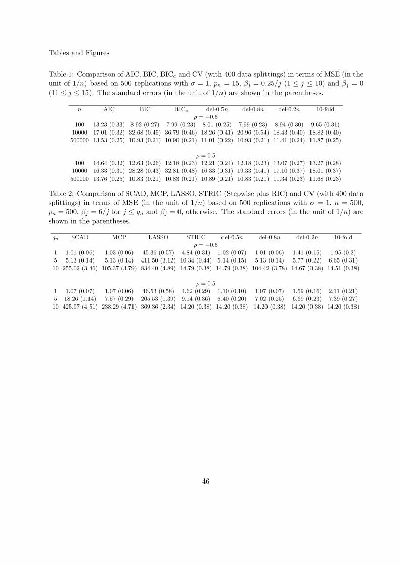
Tables and Figures

Table 1: Comparison of AIC, BIC, BICc and CV (with 400 data splittings) in terms of MSE (in theunit of 1/n) based on 500 replications with σ = 1, pn = 15, βj = 0.25/j (1 ≤ j ≤ 10) and βj = 0(11 ≤ j ≤ 15). The standard errors (in the unit of 1/n) are shown in the parentheses.

n AIC BIC BICc del-0.5n del-0.8n del-0.2n 10-fold

ρ = −0.5

100 13.23 (0.33) 8.92 (0.27) 7.99 (0.23) 8.01 (0.25) 7.99 (0.23) 8.94 (0.30) 9.65 (0.31)

10000 17.01 (0.32) 32.68 (0.45) 36.79 (0.46) 18.26 (0.41) 20.96 (0.54) 18.43 (0.40) 18.82 (0.40)

500000 13.53 (0.25) 10.93 (0.21) 10.90 (0.21) 11.01 (0.22) 10.93 (0.21) 11.41 (0.24) 11.87 (0.25)

ρ = 0.5

100 14.64 (0.32) 12.63 (0.26) 12.18 (0.23) 12.21 (0.24) 12.18 (0.23) 13.07 (0.27) 13.27 (0.28)

10000 16.33 (0.31) 28.28 (0.43) 32.81 (0.48) 16.33 (0.31) 19.33 (0.41) 17.10 (0.37) 18.01 (0.37)

500000 13.76 (0.25) 10.83 (0.21) 10.83 (0.21) 10.89 (0.21) 10.83 (0.21) 11.34 (0.23) 11.68 (0.23)

Table 2: Comparison of SCAD, MCP, LASSO, STRIC (Stepwise plus RIC) and CV (with 400 datasplittings) in terms of MSE (in the unit of 1/n) based on 500 replications with σ = 1, n = 500,pn = 500, βj = 6/j for j ≤ qn and βj = 0, otherwise. The standard errors (in the unit of 1/n) areshown in the parentheses.

qn SCAD MCP LASSO STRIC del-0.5n del-0.8n del-0.2n 10-fold

ρ = −0.5

1 1.01 (0.06) 1.03 (0.06) 45.36 (0.57) 4.84 (0.31) 1.02 (0.07) 1.01 (0.06) 1.41 (0.15) 1.95 (0.2)

5 5.13 (0.14) 5.13 (0.14) 411.50 (3.12) 10.34 (0.44) 5.14 (0.15) 5.13 (0.14) 5.77 (0.22) 6.65 (0.31)

10 255.02 (3.46) 105.37 (3.79) 834.40 (4.89) 14.79 (0.38) 14.79 (0.38) 104.42 (3.78) 14.67 (0.38) 14.51 (0.38)

ρ = 0.5

1 1.07 (0.07) 1.07 (0.06) 46.53 (0.58) 4.62 (0.29) 1.10 (0.10) 1.07 (0.07) 1.59 (0.16) 2.11 (0.21)

5 18.26 (1.14) 7.57 (0.29) 205.53 (1.39) 9.14 (0.36) 6.40 (0.20) 7.02 (0.25) 6.69 (0.23) 7.39 (0.27)

10 425.97 (4.51) 238.29 (4.71) 369.36 (2.34) 14.20 (0.38) 14.20 (0.38) 14.20 (0.38) 14.20 (0.38) 14.20 (0.38)

46

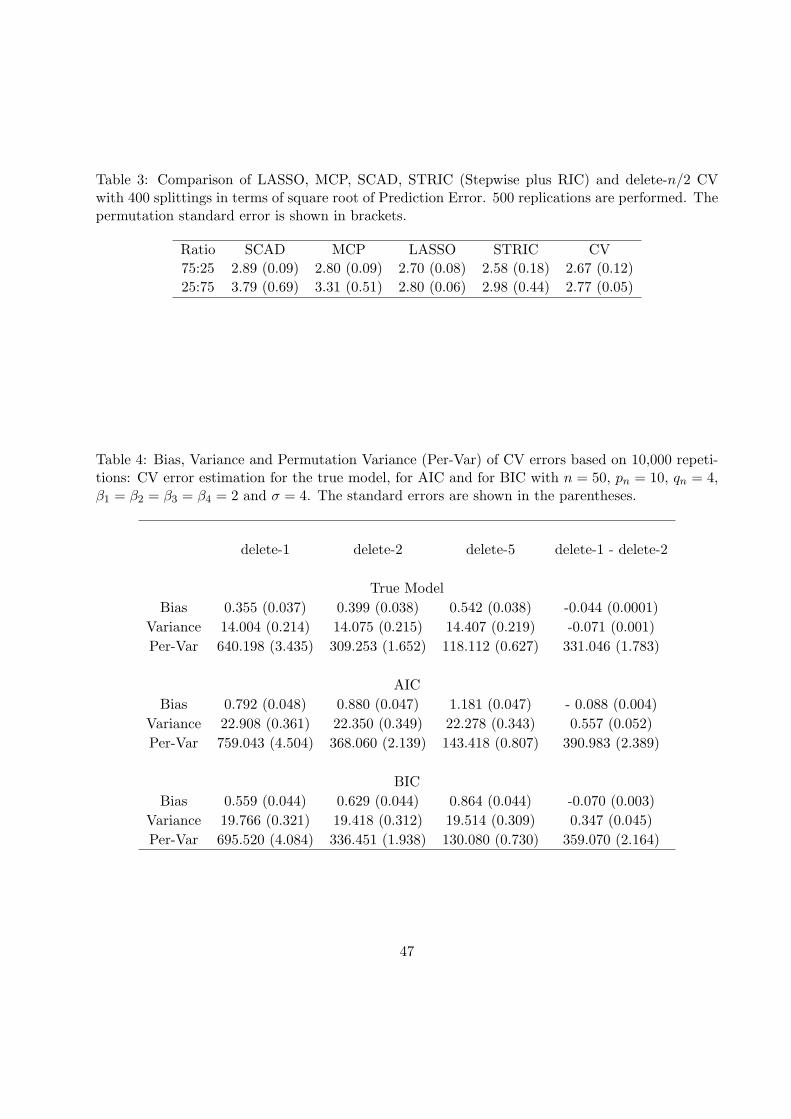
Table 3: Comparison of LASSO, MCP, SCAD, STRIC (Stepwise plus RIC) and delete-n/2 CVwith 400 splittings in terms of square root of Prediction Error. 500 replications are performed. Thepermutation standard error is shown in brackets.

Ratio SCAD MCP LASSO STRIC CV

75:25 2.89 (0.09) 2.80 (0.09) 2.70 (0.08) 2.58 (0.18) 2.67 (0.12)

25:75 3.79 (0.69) 3.31 (0.51) 2.80 (0.06) 2.98 (0.44) 2.77 (0.05)

Table 4: Bias, Variance and Permutation Variance (Per-Var) of CV errors based on 10,000 repeti-tions: CV error estimation for the true model, for AIC and for BIC with n = 50, pn = 10, qn = 4,β1 = β2 = β3 = β4 = 2 and σ = 4. The standard errors are shown in the parentheses.

delete-1 delete-2 delete-5 delete-1 - delete-2

True Model

Bias 0.355 (0.037) 0.399 (0.038) 0.542 (0.038) -0.044 (0.0001)

Variance 14.004 (0.214) 14.075 (0.215) 14.407 (0.219) -0.071 (0.001)

Per-Var 640.198 (3.435) 309.253 (1.652) 118.112 (0.627) 331.046 (1.783)

AIC

Bias 0.792 (0.048) 0.880 (0.047) 1.181 (0.047) - 0.088 (0.004)

Variance 22.908 (0.361) 22.350 (0.349) 22.278 (0.343) 0.557 (0.052)

Per-Var 759.043 (4.504) 368.060 (2.139) 143.418 (0.807) 390.983 (2.389)

BIC

Bias 0.559 (0.044) 0.629 (0.044) 0.864 (0.044) -0.070 (0.003)

Variance 19.766 (0.321) 19.418 (0.312) 19.514 (0.309) 0.347 (0.045)

Per-Var 695.520 (4.084) 336.451 (1.938) 130.080 (0.730) 359.070 (2.164)

47

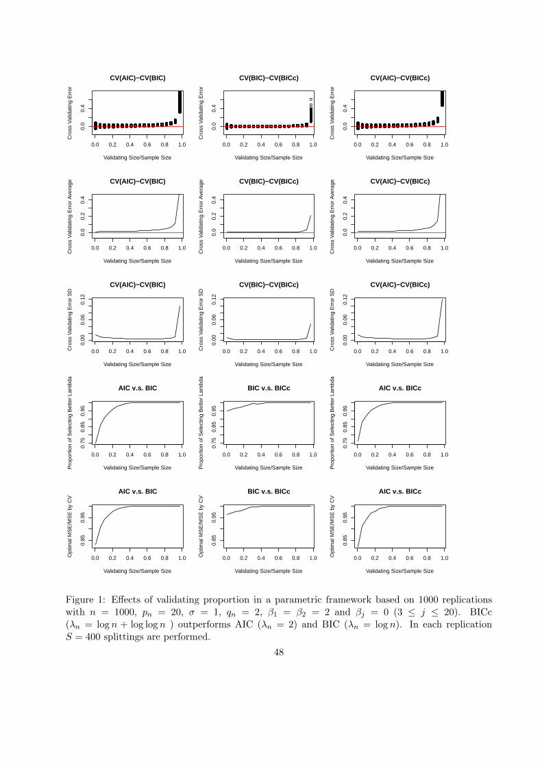
0.0 0.2 0.4 0.6 0.8 1.0

0.0

0.4

CV(AIC)−CV(BIC)

Validating Size/Sample Size

Cro

ss V

alid

atin

g E

rror

0.0 0.2 0.4 0.6 0.8 1.0

0.0

0.4

CV(BIC)−CV(BICc)

Validating Size/Sample Size

Cro

ss V

alid

atin

g E

rror

0.0 0.2 0.4 0.6 0.8 1.0

0.0

0.4

CV(AIC)−CV(BICc)

Validating Size/Sample Size

Cro

ss V

alid

atin

g E

rror

0.0 0.2 0.4 0.6 0.8 1.0

0.0

0.2

0.4

CV(AIC)−CV(BIC)

Validating Size/Sample Size

Cro

ss V

alid

atin

g E

rror

Ave

rage

0.0 0.2 0.4 0.6 0.8 1.0

0.0

0.2

0.4

CV(BIC)−CV(BICc)

Validating Size/Sample Size

Cro

ss V

alid

atin

g E

rror

Ave

rage

0.0 0.2 0.4 0.6 0.8 1.0

0.0

0.2

0.4

CV(AIC)−CV(BICc)

Validating Size/Sample Size

Cro

ss V

alid

atin

g E

rror

Ave

rage

0.0 0.2 0.4 0.6 0.8 1.0

0.00

0.06

0.12

CV(AIC)−CV(BIC)

Validating Size/Sample Size

Cro

ss V

alid

atin

g E

rror

SD

0.0 0.2 0.4 0.6 0.8 1.0

0.00

0.06

0.12

CV(BIC)−CV(BICc)

Validating Size/Sample Size

Cro

ss V

alid

atin

g E

rror

SD

0.0 0.2 0.4 0.6 0.8 1.00.

000.

060.

12

CV(AIC)−CV(BICc)

Validating Size/Sample Size

Cro

ss V

alid

atin

g E

rror

SD

0.0 0.2 0.4 0.6 0.8 1.0

0.75

0.85

0.95

AIC v.s. BIC

Validating Size/Sample SizePro

port

ion

of S

elec

ting

Bet

ter

Lam

bda

0.0 0.2 0.4 0.6 0.8 1.0

0.75

0.85

0.95

BIC v.s. BICc

Validating Size/Sample SizePro

port

ion

of S

elec

ting

Bet

ter

Lam

bda

0.0 0.2 0.4 0.6 0.8 1.0

0.75

0.85

0.95

AIC v.s. BICc

Validating Size/Sample SizePro

port

ion

of S

elec

ting

Bet

ter

Lam

bda

0.0 0.2 0.4 0.6 0.8 1.0

0.85

0.95

AIC v.s. BIC

Validating Size/Sample Size

Opt

imal

MS

E/M

SE

by

CV

0.0 0.2 0.4 0.6 0.8 1.0

0.85

0.95

BIC v.s. BICc

Validating Size/Sample Size

Opt

imal

MS

E/M

SE

by

CV

0.0 0.2 0.4 0.6 0.8 1.0

0.85

0.95

AIC v.s. BICc

Validating Size/Sample Size

Opt

imal

MS

E/M

SE

by

CV

Figure 1: Effects of validating proportion in a parametric framework based on 1000 replicationswith n = 1000, pn = 20, σ = 1, qn = 2, β1 = β2 = 2 and βj = 0 (3 ≤ j ≤ 20). BICc(λn = log n + log log n ) outperforms AIC (λn = 2) and BIC (λn = log n). In each replicationS = 400 splittings are performed.

48

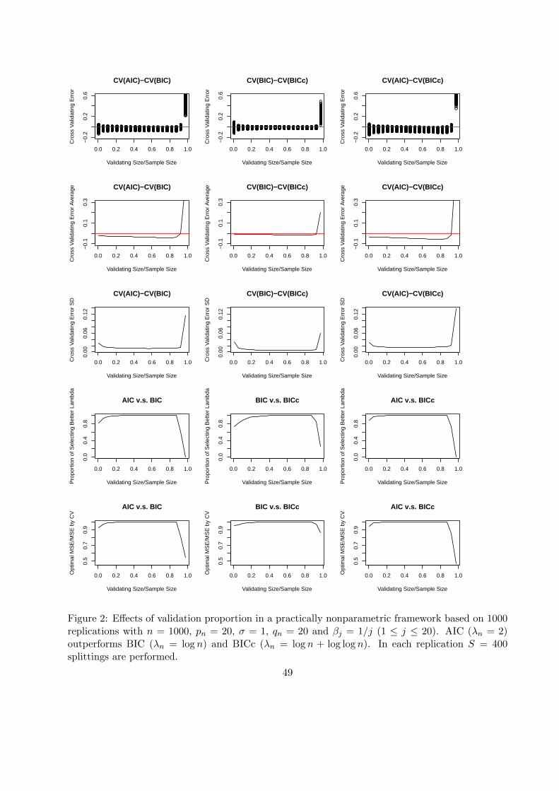
0.0 0.2 0.4 0.6 0.8 1.0

−0.

20.

20.

6CV(AIC)−CV(BIC)

Validating Size/Sample Size

Cro

ss V

alid

atin

g E

rror

0.0 0.2 0.4 0.6 0.8 1.0

−0.

20.

20.

6

CV(BIC)−CV(BICc)

Validating Size/Sample Size

Cro

ss V

alid

atin

g E

rror

0.0 0.2 0.4 0.6 0.8 1.0

−0.

20.

20.

6

CV(AIC)−CV(BICc)

Validating Size/Sample Size

Cro

ss V

alid

atin

g E

rror

0.0 0.2 0.4 0.6 0.8 1.0

−0.

10.

10.

3

CV(AIC)−CV(BIC)

Validating Size/Sample Size

Cro

ss V

alid

atin

g E

rror

Ave

rage

0.0 0.2 0.4 0.6 0.8 1.0

−0.

10.

10.

3

CV(BIC)−CV(BICc)

Validating Size/Sample Size

Cro

ss V

alid

atin

g E

rror

Ave

rage

0.0 0.2 0.4 0.6 0.8 1.0

−0.

10.

10.

3

CV(AIC)−CV(BICc)

Validating Size/Sample Size

Cro

ss V

alid

atin

g E

rror

Ave

rage

0.0 0.2 0.4 0.6 0.8 1.0

0.00

0.06

0.12

CV(AIC)−CV(BIC)

Validating Size/Sample Size

Cro

ss V

alid

atin

g E

rror

SD

0.0 0.2 0.4 0.6 0.8 1.0

0.00

0.06

0.12

CV(BIC)−CV(BICc)

Validating Size/Sample Size

Cro

ss V

alid

atin

g E

rror

SD

0.0 0.2 0.4 0.6 0.8 1.00.

000.

060.

12

CV(AIC)−CV(BICc)

Validating Size/Sample Size

Cro

ss V

alid

atin

g E

rror

SD

0.0 0.2 0.4 0.6 0.8 1.0

0.0

0.4

0.8

AIC v.s. BIC

Validating Size/Sample SizePro

port

ion

of S

elec

ting

Bet

ter

Lam

bda

0.0 0.2 0.4 0.6 0.8 1.0

0.0

0.4

0.8

BIC v.s. BICc

Validating Size/Sample SizePro

port

ion

of S

elec

ting

Bet

ter

Lam

bda

0.0 0.2 0.4 0.6 0.8 1.0

0.0

0.4

0.8

AIC v.s. BICc

Validating Size/Sample SizePro

port

ion

of S

elec

ting

Bet

ter

Lam

bda

0.0 0.2 0.4 0.6 0.8 1.0

0.5

0.7

0.9

AIC v.s. BIC

Validating Size/Sample Size

Opt

imal

MS

E/M

SE

by

CV

0.0 0.2 0.4 0.6 0.8 1.0

0.5

0.7

0.9

BIC v.s. BICc

Validating Size/Sample Size

Opt

imal

MS

E/M

SE

by

CV

0.0 0.2 0.4 0.6 0.8 1.0

0.5

0.7

0.9

AIC v.s. BICc

Validating Size/Sample Size

Opt

imal

MS

E/M

SE

by

CV

Figure 2: Effects of validation proportion in a practically nonparametric framework based on 1000replications with n = 1000, pn = 20, σ = 1, qn = 20 and βj = 1/j (1 ≤ j ≤ 20). AIC (λn = 2)outperforms BIC (λn = log n) and BICc (λn = log n + log log n). In each replication S = 400splittings are performed.

49

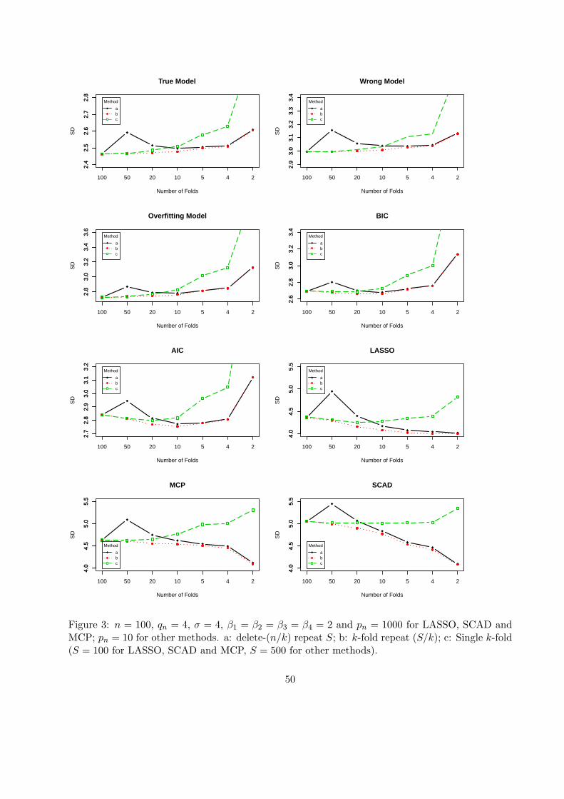
2.4

2.5

2.6

2.7

2.8

Number of Folds

SD

100 50 20 10 5 4 2

2.4

2.5

2.6

2.7

2.8

Method

abc

True Model

2.9

3.0

3.1

3.2

3.3

3.4

Number of Folds

SD

100 50 20 10 5 4 2

2.9

3.0

3.1

3.2

3.3

3.4

Method

abc

Wrong Model2.

83.

03.

23.

43.

6

Number of Folds

SD

100 50 20 10 5 4 2

2.8

3.0

3.2

3.4

3.6

Method

abc

Overfitting Model

2.6

2.8

3.0

3.2

3.4

Number of Folds

SD

100 50 20 10 5 4 2

2.6

2.8

3.0

3.2

3.4

Method

abc

BIC

2.7

2.8

2.9

3.0

3.1

3.2

Number of Folds

SD

100 50 20 10 5 4 2

2.7

2.8

2.9

3.0

3.1

3.2

Method

abc

AIC

4.0

4.5

5.0

5.5

Number of Folds

SD

100 50 20 10 5 4 2

4.0

4.5

5.0

5.5

Method

abc

LASSO

4.0

4.5

5.0

5.5

Number of Folds

SD

100 50 20 10 5 4 2

4.0

4.5

5.0

5.5

Method

abc

MCP

4.0

4.5

5.0

5.5

Number of Folds

SD

100 50 20 10 5 4 2

4.0

4.5

5.0

5.5

Method

abc

SCAD

Figure 3: n = 100, qn = 4, σ = 4, β1 = β2 = β3 = β4 = 2 and pn = 1000 for LASSO, SCAD andMCP; pn = 10 for other methods. a: delete-(n/k) repeat S; b: k-fold repeat (S/k); c: Single k-fold(S = 100 for LASSO, SCAD and MCP, S = 500 for other methods).

50

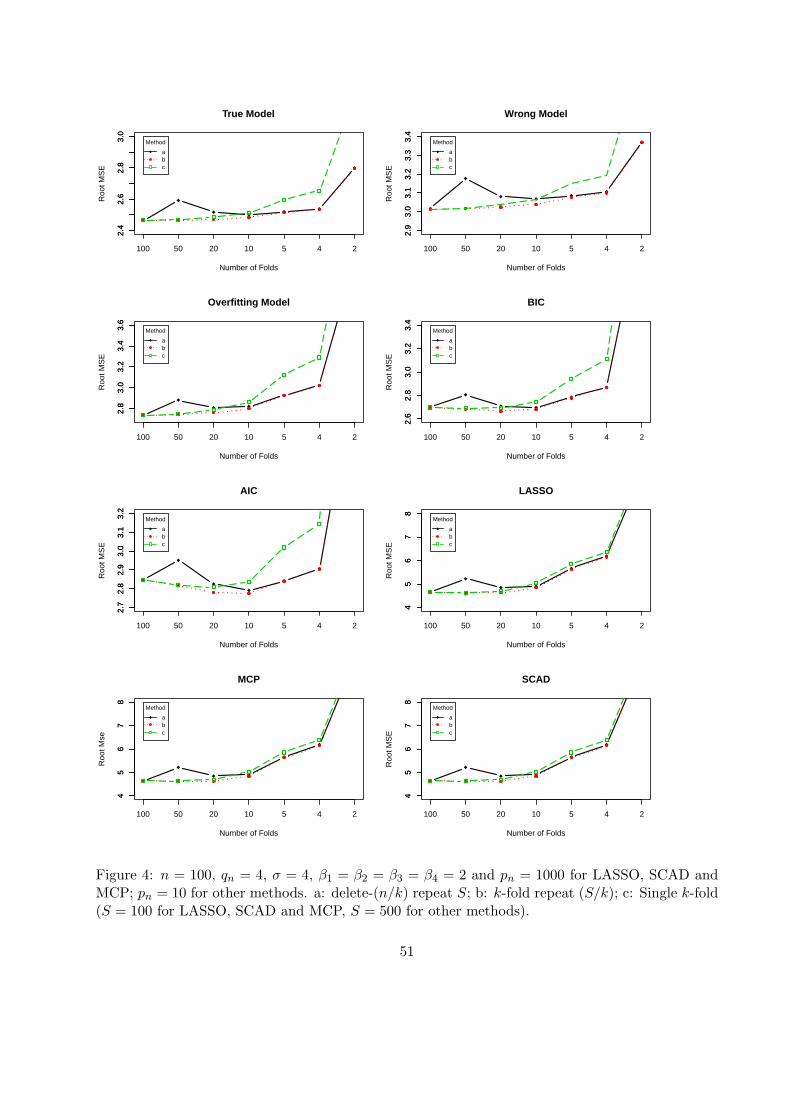
2.4

2.6

2.8

3.0

Number of Folds

Roo

t MS

E

100 50 20 10 5 4 2

2.4

2.6

2.8

3.0

Method

abc

True Model

2.9

3.0

3.1

3.2

3.3

3.4

Number of Folds

Roo

t MS

E

100 50 20 10 5 4 2

2.9

3.0

3.1

3.2

3.3

3.4

Method

abc

Wrong Model2.

83.

03.

23.

43.

6

Number of Folds

Roo

t MS

E

100 50 20 10 5 4 2

2.8

3.0

3.2

3.4

3.6

Method

abc

Overfitting Model

2.6

2.8

3.0

3.2

3.4

Number of Folds

Roo

t MS

E

100 50 20 10 5 4 2

2.6

2.8

3.0

3.2

3.4

Method

abc

BIC

2.7

2.8

2.9

3.0

3.1

3.2

Number of Folds

Roo

t MS

E

100 50 20 10 5 4 2

2.7

2.8

2.9

3.0

3.1

3.2

Method

abc

AIC

45

67

8

Number of Folds

Roo

t MS

E

100 50 20 10 5 4 2

45

67

8

Method

abc

LASSO

45

67

8

Number of Folds

Roo

t Mse

100 50 20 10 5 4 2

45

67

8

Method

abc

MCP

45

67

8

Number of Folds

Roo

t MS

E

100 50 20 10 5 4 2

45

67

8

Method

abc

SCAD

Figure 4: n = 100, qn = 4, σ = 4, β1 = β2 = β3 = β4 = 2 and pn = 1000 for LASSO, SCAD andMCP; pn = 10 for other methods. a: delete-(n/k) repeat S; b: k-fold repeat (S/k); c: Single k-fold(S = 100 for LASSO, SCAD and MCP, S = 500 for other methods).

51

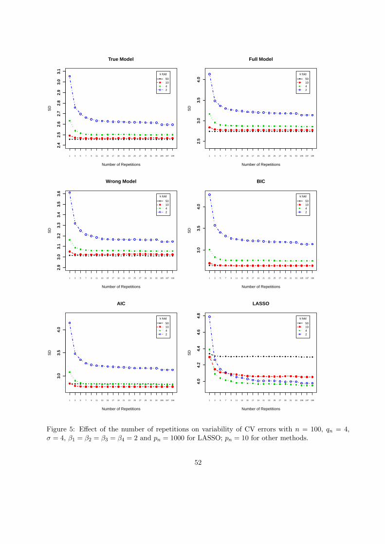
2.4

2.5

2.6

2.7

2.8

2.9

3.0

3.1

Number of Repetitions

SD

1 3 5 7 9 11 13 15 17 19 21 23 25 27 29 31 33 195 197 199

2.4

2.5

2.6

2.7

2.8

2.9

3.0

3.1

k fold

501042

True Model

2.5

3.0

3.5

4.0

Number of Repetitions

SD

1 3 5 7 9 11 13 15 17 19 21 23 25 27 29 31 33 195 197 199

2.5

3.0

3.5

4.0

k fold

501042

Full Model2.

93.

03.

13.

23.

33.

43.

53.

6

Number of Repetitions

SD

1 3 5 7 9 11 13 15 17 19 21 23 25 27 29 31 33 195 197 199

2.9

3.0

3.1

3.2

3.3

3.4

3.5

3.6

k fold

501042

Wrong Model

3.0

3.5

4.0

Number of Repetitions

SD

1 3 5 7 9 11 13 15 17 19 21 23 25 27 29 31 33 195 197 199

3.0

3.5

4.0

k fold

501042

BIC

3.0

3.5

4.0

Number of Repetitions

SD

1 3 5 7 9 11 13 15 17 19 21 23 25 27 29 31 33 195 197 199

3.0

3.5

4.0

k fold

501042

AIC

4.0

4.2

4.4

4.6

4.8

Number of Repetitions

SD

1 3 5 7 9 11 13 15 17 19 21 23 25 27 29 31 33 195 197 199

4.0

4.2

4.4

4.6

4.8

k fold

501042

LASSO

Figure 5: Effect of the number of repetitions on variability of CV errors with n = 100, qn = 4,σ = 4, β1 = β2 = β3 = β4 = 2 and pn = 1000 for LASSO; pn = 10 for other methods.

52