Cross-Virtual Concatenation for

Ethernet-over-SONET/SDH Networks

Satyajeet S. Ahuja and Marwan Krunz

Department of Electrical and Computer Engineering

The University of Arizona, Tucson, AZ 85721

{ahuja,krunz}@ece.arizona.edu

Abstract

Ethernet-over-SONET/SDH (EoS) is a popular approach for interconnecting geographically distant Ethernet

segments using a SONET/SDH transport infrastructure. It typically uses virtual concatenation (VC) for dynamic

bandwidth management. The aggregate SONET/SDH bandwidth for a given EoS connection is obtained by

“concatenating” a number of equal-capacity virtual channels. Together, these virtual channels form a virtually

concatenated group (VCG). In this paper, we introduce a new concatenation technique, referred to as cross-virtual

concatenation (CVC), which involves the concatenation of virtual channels of heterogeneous capacities. We show

that CVC can be implemented through a simple upgrade at the end node, thus utilizing the existing legacy

SDH infrastructure. By employing CVC for EoS systems, we show that the SDH bandwidth can be harvested

more efficiently than in conventional VC. We consider two problems associated with routing CVC connections:

the connection establishment problem and the connection upgrade problem. The goal of the first problem is to

compute a set of paths between two EoS end systems such that a total bandwidth demand and a constraint on

the differential delay between the paths are satisfied. Among all feasible sets, the one that consumes the least

amount of network bandwidth is selected. For this problem, we develop an integer linear program (ILP) and an

efficient algorithm based on the sliding-window approach. For the connection upgrade problem, the goal is to

augment an existing set of paths so as to increase the aggregate bandwidth while continue to meet the differential-

delay constraint. We model this problem as a flow-maximization problem with a constraint on the delay of the

virtual channels with positive flow. We then consider the problem of path selection under imprecise network state

information. Simulations are conducted to demonstrate the advantages of employing CVC and to evaluate the

performance of the proposed algorithms.

1. Introduction

The current optical transport infrastructure is dominated by the SONET/SDH technology [1, 2]. SDH uses a

bandwidth hierarchy indicated by STM-n, where n = 1, 4, 16, 64, . . .. The basic unit in this hierarchy is the STM-1

channel (155.52 Mbps), which can support various smaller payloads, including VC-11 (1.5 Mbps), VC-12 (2 Mbps),

and VC-3 (45 Mbps). SDH was originally developed to support voice traffic. As the demand for “data” services (IP

and Ethernet traffic) continued to rise, it became imperative to provide cost-effective solutions for supporting such

services over the SDH infrastructure. One popular solution is based on Ethernet-over-SONET/SDH (EoS), which

enables a network provider to interconnect Ethernet LANs over regional and even transcontinental distances [3, 4, 5].

1

EoS facilitates the provisioning of various data services, such as the Ethernet-private-leased-line service (which

supports dedicated point-to-point bandwidth) and the Ethernet-virtual-private-line service (which uses statistical

multiplexing for bandwidth sharing among various traffic streams).

In EoS, the aggregate bandwidth needed to interconnect two Ethernet segments is typically obtained by virtually

concatenating several SDH payloads (VC-n channels) that possibly belong to different optical carriers (STM-ns) [2].

An example of two optical carriers containing virtually concatenated payloads is shown in Figure 1. The two carriers

are routed along two different paths, whose delays are denoted by D1 and D2, respectively. The differential delay

between these two paths is |D1 −D2|. The two paths represent two virtual channels. Together, they form a virtually

Ethernet 1 Ethernet 2

Figure 1: EoS setup with conventional virtual concatenation.

concatenated group (VCG). Different members of a VCG may be assigned noncontiguous slots within an SDH frame,

and they can be routed independently. In conventional virtual concatenation, the virtual channels of a VCG are of

the same SDH payload capacity. For a VCG of k virtual channels, the source node splits the traffic equally among

the k channels. The data is byte-interleaved, e.g., if the first byte is transmitted on the rth virtual channel, then the

next byte is transmitted on the (r + 1)th virtual channel, and so on. Control information is embedded in overhead

bytes (known as path overhead) associated with each virtual channel. The receiving end-point is responsible for

re-assembling the original byte stream and compensating for the differential delay between the different paths taken

by the virtual channels. This is done using a very high-speed memory. Once the SDH frames of all virtual channels

that have the same frame number (i.e., time-stamp) have arrived at the destination node, Ethernet frames can be

reconstructed. It is obvious that the higher the differential delay, the larger the memory requirement. Only the

two end-points need to support VC [2]. By using the link capacity adjustment scheme (LCAS) [6], VC can support

dynamic link upgrade and on-demand bandwidth adjustment without requiring additional hardware.

While the use of virtually concatenated EoS circuits for Ethernet transport enables efficient utilization of the

SDH bandwidth, it may result in a large number of virtual channels between the two end-points. For example,

consider the two Ethernet LANs in Figure 2, with an aggregate traffic demand of 100 Mbps. The two LANs can

be connected by employing fifty VC-12 channels. This large number of circuits involves high maintenance overhead.

The SDH bandwidth that is needed to support fifty VC-12 channels is actually greater than 100 Mbps. Specifically,

the hierarchical implementation of an SDH frame [2] allows for a maximum of 21 VC-12 channels over a TUG-3

(tributary unit group) of an STM-1 frame. So, fifty VC-12 channels are transported using 45+45+(8/21)×45 =

107 Mbps of actual bandwidth. An alternative is to employ three VC-3 channels (3×45 Mbps = 135 Mbps), at the

expense of excessive bandwidth wastage.

To improve bandwidth utilization while employing a relatively small number of connections, an EoS system needs

to be able to combine virtual channels of different payloads in the same VCG. For example, the 100 Mbps traffic can

be supported using two VC-3 channels (90 Mbps) and five VC-12 channels (10 Mbps). The actual SDH bandwidth

2

SDH

Node

SDH

Node

SDH

Node

SDH

Node

Conventional virtual concatenation using 50xVC-12s results in bandwidth fragmentation

Conventional virtual concatenation using 3xVC-3s results in bandwidth wastage

SDH

Node

SDH

Node

Cross-virtual concatenation using 2xVC-3s and 5xVC-12s maintains bandwidth efficiency

and reduces the number of circuits

Figure 2: Example that demonstrates the advantages of CVC.

that will be consumed in this case is 101.9 Mbps (2×45 + (5/21)×45). We refer to the concatenation of SDH channels

of different payload capacities as cross-virtual concatenation (CVC). By employing CVC, we are able to harvest the

SDH bandwidth more efficiently. We later show that the gain achieved by employing CVC increases linearly with

the VCG bandwidth demand.

In this paper, we outline the general structure of the proposed CVC approach (Section 2) and describe its

advantages over conventional virtual concatenation. We show a typical implementation of CVC based on VC-12 and

VC-3 payloads. This implementation exploits control information already available in the SDH frame. It requires

a simple end-point upgrade. We study two path selection problems associated with interconnecting two EoS end-

points via CVC. The first problem is that of establishing an EoS connection with a given bandwidth demand (Section

3). In this problem, the goal is to compute a set of paths that satisfy the given bandwidth demand and a given

differential delay constraint, and that consumes the least amount of network bandwidth. We present an integer

linear programming (ILP) formulation and an efficient algorithm to solve the connection establishment problem.

The presented algorithm converts the problem into a flow-maximization problem and uses a modified version of

the sliding-window approach [7] to find a feasible set of paths. We then consider the problem of augmenting an

existing EoS connection in order to increase its aggregate bandwidth (Section 4). This problem is modelled as a

flow-maximization problem with a two-sided delay constraint. We use the modified-link-weight K-shortest path

(MLW-KSP) algorithm described [8] to compute the two-sided constrained paths. From these paths, we sequentially

choose a set of paths that can satisfy the bandwidth and delay constraints. We also study the path selection problem

when the information about link delays and bandwidth availability is not precisely known at the time of path selection

(Section 5). We propose an algorithm based on the “backward forward” approach to solve this problem. We study

the performance of the proposed algorithms (Section 6) and compare them with path selection under conventional

virtual concatenation.

2. Implementation of Cross-Virtual Concatenation

In this section, we describe how CVC can be implemented via a simple end-point upgrade. For illustration purposes,

we describe a particular instance of CVC, applied to the concatenation of VC-3 and VC-12 channels. However, the

concept can be easily generalized for multiple payloads of different capacities. The implementation described in this

section is divided into two parts: transmit side and receive side. This implementation is similar to a classic VC

implementation but with a different mechanism for payload splitting and assembly.

3

2.1 Transmit Side

In a typical transmit-side implementation of EoS, Ethernet frames are encapsulated using the generic framing proce-

dure (GFP) [9, 10] or the link access protocol-SDH (LAP-S) [2]. The resultant stream of bytes is then interleaved into

the various members of the VCG. In the CVC implementation (see Figure 3), we use a special payload splitter and a

buffer assembly, just after frame encapsulation. The splitter consists of a set of payload counters that are associated

GFP

PAYLOAD SPLITTER

SONET FRAME

Ethernet Frames

Payload Buffer

Figure 3: Transmit-side implementation of CVC.

with various payload types (VC-12, VC-3, etc.). A payload-select counter is used to choose the appropriate buffer

for storing the incoming payload. Each payload counter maintains the number of bytes of a particular payload type

present in an SDH frame. For example, if there are n VC-12 channels in a VCG, then the VC-12 payload counter

counts from 0 to 34n− 1 (there are 34 bytes of payload data in a VC-12 channel per SDH frame). Similarly, if there

are m VC-3 channels in a VCG, the VC-3 payload counter counts from 0 to 765m− 1 (there are 765 bytes of payload

data in a VC-3 channel per SDH frame). The payload-select counter counts from 0 to J − 1, where J is the number

of payload types participating in CVC; in this case two (VC-3s and VC-12s). The various states of the payload-select

counter are used to generate enable signals for various payload counters. At any instant, only one payload counter

is enabled.

There are J buffers (one for each payload type) for storing incoming payload bytes. When a byte is received from

the GFP encapsulator, it is stored into the payload buffer for which the write enable signal is high. The various

virtual channels are fed from their respective buffers. Figure 4 depicts a timing diagram for the various counters.

For example, in a CVC of one VC-3 and one VC-12 channels, there are 799 bytes per SDH frame. The first 765

bytes are stored in the VC-3 payload buffer and the next 34 bytes are stored in the VC-12 payload buffer. The

splitting of payloads ensures that the ratio of traffic transmitted over different payload types is the same as the ratio

of the number of bytes transmitted over each payload type in an SDH frame. As discussed later, such splitting does

not add any complexity at the receiver. The multi-frame and sequence numbers are used in the same way as in

conventional VC. For example, the sequence number for the n VC-12 channels ranges from 0 to n − 1, and for the

4

VC-12 Payload Counter

VC-3 Payload Counter

Counts from 0 to 34*n -1

Payload Select Counter and VC-3 Payload Buffer write_enable

Counts from 0 to 765*m-1

VC-12 Payload Buffer write_enable

Figure 4: Timing diagram of various counters for the transmit-side implementation of CVC.

m VC-3 channels it ranges from 0 to m − 1. If there are multiple VC-3 or VC-12 channels, then as in conventional

virtual concatenation, the payloads stored in different payload buffers are byte-interleaved when inserted into the

SDH frame.

Each buffer is essentially a FIFO queue. After splitting, the data is written to the end of these queues. For

a given VCG, the total amount of buffer needed to store the payload bytes is twice the number of bytes that are

actually transmitted on the SDH frame. Two-frame worth of storage capacity is needed to maintain exclusion in read

and write memory operations. In the worst case, buffering introduces an additional delay of 250 µsec (equivalent to

the transmission time of two SDH frames). Since the complete data stream is delayed by a constant amount, such

buffering does not add any extra complexity in the receive side.

2.2 Receive Side

In a typical receive-side implementation of EoS, the received SDH payload is stored in a differential delay compensator,

which is essentially a buffer. Once the frames of all members of the VCG with the same frame number (time-stamp)

have arrived, the payload bytes are sequentially removed from the buffer according to their sequence numbers, and

are inputed to the GFP decapsulator. In a CVC implementation, we use different buffers for different payload types

to compensate for the differential delay. Once the payloads of all the members of the VCG with the same frame

number have arrived, the payload assembler sequentially extracts the various payload bytes. The assembler contains

a set of counters that provide the appropriate addresses for fetching the payload bytes from the corresponding buffers

(see Figure 5). The payload buffer also generates the payload-select signal, which is used as the select line of the

multiplexer. The multiplexer chooses the correct payload bytes to be sent to the GFP module. An address generator

generates appropriate read addresses for the payload buffers.

Note that the implementation of CVC described above does not require intermediate nodes along a path of a

VC-n channel to be aware of the CVC connection. These intermediate nodes treat this VC-n as any other VC-n

channel. Hence, implementing CVC requires hardware upgrade at the end nodes only.

5

Payload Select Signal

VC-12 Payload Buffer

VC-3 Payload Buffer

Address Generator

MUX

Address Bits

Payload Data

Data Input Data Input

Address Bits

Figure 5: Receive-side implementation of CVC.

3. Connection Establishment Under CVC

In this section, we consider the problem of establishing a new CVC connection. Consider two remotely separated

Ethernet LANs that need to be connected using EoS with a total bandwidth requirement RB . Let s and t be the two

SDH end points. The goal is to find a set of paths between s and t that supports the required aggregate bandwidth,

that satisfies a differential delay requirement, and that consumes the minimum possible network bandwidth. Note

that while the paths that comprise the CVC connection may differ in their payloads, each path supports the same

payload over all of its links. Before proceeding further, we define the following parameters:

• Sn: Actual bandwidth consumed by a VC-n channel within an SDH frame. For example, an STM-1 frame

can transport three VC-3 channels. Hence, S3 = 155/3 = 51.66 Mbps. Similarly, S12 = 155/63 = 2.46 Mbps

for a VC-12 channel, and S4 = 155/1 = 155 Mbps for a VC-4 channel. Note that Sn includes the overhead

associated with transporting a given virtual channel within the SDH frame structure.

• IBn: Payload bandwidth of a VC-n channel, i.e., the bandwidth associated with the user’s data (IB3 = 45 Mbps

for a VC-3 channel, IB12 = 2 Mbps for a VC-12 channel, and IB4 = 140 Mbps for a VC-4 channel).

• Buv: Total payload bandwidth available over a link (u, v); Buv =∑

n IBnbn(u, v), where bn(u, v) is the number

of unused VC-n channels over link (u, v).

The total amount of network resources consumed by a path P of h(P ) hops and of total connection bandwidth f(P )

is given by h(P )f(P ). Moreover, if a path P is chosen for routing a VC-n channel then this channel is reserved along

all the links of path P .

We now formally define the connection establishment problem.

Problem 1 Connection Establishment (CE): Consider an SDH network that is modeled as a graph G(N ,L), where

each link (u, v) ∈ L is associated with a total available payload capacity Buv =∑

n IBnbn(u, v) and delay w(u, v).

Find a set of paths between source s and destination t such that: (1) the aggregate capacity of these paths is greater

than or equal to RB, (2) the maximum differential delay between two paths in the selected set is less than a given

constant △, and (3) the bandwidth of the selected paths is minimum among all feasible sets of paths that satisfy (1)

and (2).

6

The example in Figure 6 illustrates the CE problem. In this example, an EoS with RB = 100 Mbps is to be

established between nodes 1 and 5. For the two paths P1 = (1 − 2 − 4 − 5) and P2 = (1 − 2 − 3 − 5), the number

of available VC-3 (VC-12) channels are 2 (2) and 1 (3), respectively. Note that a single path between nodes 1

and 5 cannot support the required 100 Mbps. For simplicity, suppose that P1 and P2 satisfy the differential delay

constraint. A feasible solution involving two VC-3 channels along P1 and one VC-3 channel along P2 satisfies the

bandwidth requirement but consumes excessive network resources. A CVC solution of two VC-3 and two VC-12

channels along P1, and three VC-12 channels along P2 provides an optimal solution in this case.

1 2

3

4

5 b 12 (1,2)=15

b 12 (2,3)=3 b 12 (3,5)=7

b 12 (2,4)=2 b 12 (4,5)=7

b 3 (1,2)=3

b 3 (2,4)=2 b 3 (4,5)=2

b 3 (2,3)=1 b 3 (3,5)=4

Figure 6: Example network for the connection establishment problem.

In [7], the authors considered the differential delay routing (DDR) problem with standard virtual concatenation.

They showed that this problem is NP-complete and cannot be solved by any ǫ-approximation algorithm. The problem

addressed in our paper is even more complicated than the DDR problem, and in the best case is equivalent to it

(when only one type of payload is available). Hence, the CE problem is also NP-complete.

The CE problem can be addressed by splitting it into two parts. First, for the given network, we check the

feasibility of the requested bandwidth. If it is feasible, we then compute a set of paths that satisfy the differential

delay requirement. The first step can be solved by employing any standard maximum-flow algorithm (e.g., [11]).

The second step requires the enumeration of all the paths, and is therefore NP-hard. Instead of computing these

paths at the connection establishment time, we can precompute a set of K paths for each payload and then focus

on the problem of choosing a subset of paths from these precomputed paths that satisfies the differential delay

requirement and that has the desired total capacity with a minimum network bandwidth usage. We first propose

an ILP formulation to solve the CE problem and later propose an efficient algorithm based on the sliding-window

approach.

3.1 ILP formulation

For each payload type n, let IPn = {P(n)1 , P

(n)2 , . . . , P

(n)K } be a set of K precomputed paths that satisfy the differential

delay requirement, i.e., maxn,m |D(P(n)i ) − D(P

(m)j )| ≤ ∆, where D(P

(m)j ) is the delay associated with path P

(m)j .

Define the indicator function I(i)n (u, v) as follows: I

(i)n (u, v) = 1, if (u, v) ∈ P

(n)i , and is 0 otherwise. The set IPn is

an input to the ILP. Hence, I(i)n (u, v) is known in advance ∀(u, v) ∈ L. Let N

(i)n be an integer variable that indicates

the number of VC-n channels along path P(n)i that are in the solution set. Figure 7 depicts the ILP formulation.

Constraint C1 ensures that the chosen paths and their capacities do not violate the capacities of various links.

Notice that I(i)n (u, v)SnN

(i)n is the total bandwidth consumed by N

(i)n VC-n channels over link (u, v). Constraint C2

ensures that the solution satisfies the bandwidth requirement RB . The objective function minimizes the sum of the

bandwidth reserved by the connection request over all the links in the network.

7

Minimize:∑

(u,v)∈L

∑n

∑|IPn|i=1 {I

(i)n (u, v)SnN

(i)n }

Subject to

C1:∑

n

∑|IPn|i=1 {I

(i)n (u, v)SnN

(i)n } ≤ Buv ∀(u, v) ∈ L

C2:∑

(u,v)∈L:v=d

∑n

∑|IPn|i=1 {I

(i)n (u, v)IBnN

(i)n } ≥ RB

Figure 7: ILP formulation for the connection establishment problem.

3.2 Sliding Window Algorithm

The set of paths returned by the ILP solution minimizes the total allocated bandwidth, but its worst-case complexity

is exponential in the size of the network. Hence, we now propose a computationally efficient algorithm, which is

a variant of the sliding-window approach presented in [7]. The algorithm uses the K-shortest path algorithm [12]

to precompute a set of paths. It then sequentially tries these paths in search of a feasible solution. A pseudocode

of the Sliding-Window algorithm is presented in Figure 8. It takes as input the graph G(N ,L), the source node

s, the destination node t, the capacity requirement RB , and the differential delay constraint △. For each payload

type n, the algorithm precomputes a set of k paths IPn, ordered increasingly according to their delay values. Out

of these paths, the algorithm forms a set P = ∪nIPn, that contains the set of all paths ordered according to their

delay values. In the first iteration, the algorithm considers all the paths P1, P2, ..., Pr, where Pr ∈ P is the path

with the highest delay value such that D(Pr) − D(P1) ≤ ∆. After identifying these paths, the algorithm routes the

maximum permissible flow along these paths, starting with the path that has the minimum hop count (in case of

a tie, the path with the higher bandwidth is chosen). Note that the maximum flow f(P ) along a path P is given

by f(P ) = min(u,v)∈P Buv. The algorithm routes an amount of flow f(P ) along the chosen path P . For each link

(u, v) ∈ P , its capacity is recalculated as follows: Buv = Buv − f(P )1. If the total added capacity along all the paths

is greater than RB , the algorithm terminates.

In the jth iteration, the algorithm starts with the jth path (Pj) from the sorted list P as the first path and then

evaluates the path Pr′ as the maximum delay path in P such that D(Pr′) − D(Pj) ≤ ∆. For the same iteration,

we also maintain a set of paths Pitr, which represents all the paths under consideration during the iteration. For

example, for the jth iteration, Pitr = {Pj , Pj+1, ..., Pr′}.

Complexity: Precomputing a set of k paths for each payload type can be done in O(k|L| log(k|N |)+k2|N |) time

using the K-shortest path algorithm [12]. Let r be the number of payload types. The total complexity in computing

the set P is O(rk|L| log(k|N |) + rk2|N |). Sorting P based on hop count requires O(kr log(kr)) time. Each iteration

in Step 4 requires updating the link capacities for a maximum of rk paths and each path can have |N | hops. Hence,

the total complexity associated with each iteration is rk|N |. The Sliding-Window algorithm can have a maximum

of kr iterations. The total complexity associated with rk iterations is O(r2k2|N |). Hence, the total complexity of

the algorithm is O(rk|L| log(k|N |) + rk2|N | + kr log(kr) + r2k2|N |).

1Note that the flow along a set of paths is not the sum of the flows along the individual paths. Augmenting a flow along a path mayreduce the flow on other paths that share common links with the first path. Determining the maximum flow for a set of n paths is anNP-hard problem [13].

8

Sliding-Window(G(N ,L), s, t, w(.), B(.), IBn,△, RB)

1. Precompute K paths IPn = {P(n)1 , P

(n)2 , ..., P

(n)k } ∀ n,

ordered increasingly according to their delays.2. Set P = ∪nIPn, n = 3, 4, 12, ...3. Sort P ≡ {P1, P2, ..., P|P|} w.r.t. path delay4. For i = 1, 2,...,|P|,5. Compute Pitr = {Pi, Pi+1, ..., Pr: D(Pr) − D(Pi) ≤ ∆}6. Sort the paths in Pitr based on hop count

Resolve ties according to path capacity7. Fitr = 0, S = Φ8. For j = i, i + 1, ..., r,9. Route maximum flow f(Pj) along Pj

10. Fitr = Fitr + f(Pj), S = S ∪ {(Pj , f(Pj))}12. If Fitr > RB ,13. Return S

end For14. Set Buv ∀(u, v) ∈ L to its initial value

end For

Figure 8: Pseudocode for the Sliding-Window algorithm.

4. Connection Upgrade Problem

We now consider the connection upgrade problem. Given an established EoS connection between two LANs, we want

to upgrade it by adding RB Mbps bandwidth. The additional bandwidth can be harvested by using a cross-virtually

concatenated payloads such that the resulting flow is feasible and the consumed bandwidth is minimal.

In [8], the connection upgrade problem for the conventional virtually concatenated EoS system was studied. The

problem was reduced to a two-sided constraint path (TSCP) problem, which was heuristically solved using a modified

version of the standard K-shortest path algorithm, referred to as modified link weight K-shortest path (MLW-KSP).

TSCP was shown to be NP-complete [8]. The problem at hand is more complicated than the standard TSCP problem

because it involves multiple payload types and multiple paths. It can be thought of as a generalization of the TSCP

problem. We now formally state the connection upgrade problem:

Problem 2 Connection Upgrade (CU): Consider a graph G(N ,L), a source-destination pair (s, t), and an estab-

lished EoS connection with m members (paths) in the VCG whose respective path delays are D1,D2, . . . ,Dm. Let

△ be the maximum allowable differential delay. Each link (u, v) ∈ L is associated with a nonnegative capacity Buv.

Given a required upgrade bandwidth RB, we need to find a set of paths P between s and t that satisfies the following:

• The maximum bandwidth that can be routed along the set P is greater than RB.

• The delay associated with each path Pi ∈ P satisfies:

|D(Pi) − D(Pj)| ≤ ∆, ∀Pi, Pj ∈ P. (1)

• The delay associated with each path Pi ∈ P satisfies the differential delay constraint with all the m existing

9

members of the VCG:

max1≤j≤m

|Dj − D(Pi)| ≤ ∆, ∀Pi ∈ P. (2)

• The network resource consumed by P is minimum among all feasible solutions.

In Figure 9, we pictorially show how (2) results in a two-sided constraint (represented by a lower bound C1 and an

upper bound C2) on the delay of a new virtual channel due to the presence of existing virtual channels.

0

0 C C2

2

1

1 2

D D

D

CC

1

1

(a) m = 1

(b) m = 2

����������������������������������������������������������������������������

Figure 9: Pictorial representation of the differential delay requirement when the existing VCG contains: (a) onepath, and (b) two paths.

4.1 Upgrade Algorithm

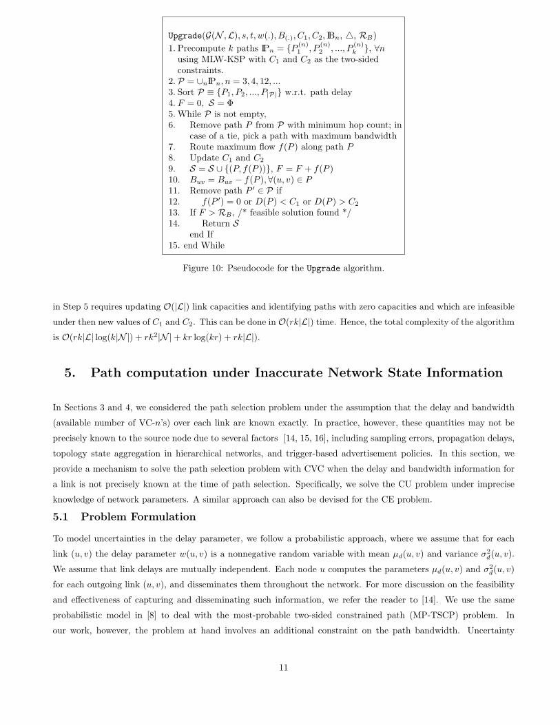
We now present an algorithm for solving the CU problem. A pseudocode for this algorithm, called Upgrade is shown

in Figure 10. Its input is the graph G(N ,L), source node s, destination node t, the required capacity upgrade

RB , the supported differential delay △, and two positive constants C1 and C2 that represent the minimum and

maximum delays of the paths in the resulting solution set S. The initial values of C1 and C2 are obtained using

the m existing members of the VCG. Specifically, C1 = max1≤i≤m(Di −△) and C2 = min1≤i≤m(Di + △). For each

payload type n, the algorithm precomputes a set of feasible paths IPn by using the MLW-KSP algorithm described

in [8]. The delay of each path P ∈ IPn satisfies C1 ≤ D(P ) ≤ C2. The MLW-KSP algorithm may return less

than k feasible paths. In that case, Upgrade explores fewer paths. The algorithm then computes the set of paths

P = ∪nIPn = {P1, P2, ..., P|P|}, sorted increasingly according to the hop count. Upgrade sequentially considers paths

in P. In case of a tie, a path with higher available capacity is picked; further ties can be resolved randomly. For a

path Pi, Upgrade performs the following:

• Routes the maximum flow f(Pi) along Pi, where f(Pi) = min(u,v)∈PiBuv.

• Recomputes the new set of constraints C1 = max(C1,D(Pi) −△) and C2 = min(C2,D(Pi) + △).

• Updates the capacity associated with the links corresponding to path Pi.

Upgrade then removes from P any path whose delay does not satisfy the differential delay constraint under the new

values of C1 and C2, or whose capacity is zero. The algorithm terminates if the bandwidth requirement is satisfied

or if the set P is empty.

Complexity: Precomputing a set of k paths for each payload type can be done in O(k|L| log(k|N |) + k2|N |)

time using the K-shortest path algorithm [12]. Let r be the total payload types. The total complexity in computing

the set P is O(rk|L| log(k|N |) + rk2|N |). Sorting P based on hop count requires O(kr log(kr)) time. Each iteration

10

Upgrade(G(N ,L), s, t, w(.), B(.), C1, C2, IBn, △, RB)

1. Precompute k paths IPn = {P(n)1 , P

(n)2 , ..., P

(n)k }, ∀n

using MLW-KSP with C1 and C2 as the two-sidedconstraints.

2. P = ∪nIPn, n = 3, 4, 12, ...3. Sort P ≡ {P1, P2, ..., P|P|} w.r.t. path delay4. F = 0, S = Φ5. While P is not empty,6. Remove path P from P with minimum hop count; in

case of a tie, pick a path with maximum bandwidth7. Route maximum flow f(P ) along path P8. Update C1 and C2

9. S = S ∪ {(P, f(P ))}, F = F + f(P )10. Buv = Buv − f(P ),∀(u, v) ∈ P11. Remove path P ′ ∈ P if12. f(P ′) = 0 or D(P ) < C1 or D(P ) > C2

13. If F > RB , /* feasible solution found */14. Return S

end If15. end While

Figure 10: Pseudocode for the Upgrade algorithm.

in Step 5 requires updating O(|L|) link capacities and identifying paths with zero capacities and which are infeasible

under then new values of C1 and C2. This can be done in O(rk|L|) time. Hence, the total complexity of the algorithm

is O(rk|L| log(k|N |) + rk2|N | + kr log(kr) + rk|L|).

5. Path computation under Inaccurate Network State Information

In Sections 3 and 4, we considered the path selection problem under the assumption that the delay and bandwidth

(available number of VC-n’s) over each link are known exactly. In practice, however, these quantities may not be

precisely known to the source node due to several factors [14, 15, 16], including sampling errors, propagation delays,

topology state aggregation in hierarchical networks, and trigger-based advertisement policies. In this section, we

provide a mechanism to solve the path selection problem with CVC when the delay and bandwidth information for

a link is not precisely known at the time of path selection. Specifically, we solve the CU problem under imprecise

knowledge of network parameters. A similar approach can also be devised for the CE problem.

5.1 Problem Formulation

To model uncertainties in the delay parameter, we follow a probabilistic approach, where we assume that for each

link (u, v) the delay parameter w(u, v) is a nonnegative random variable with mean µd(u, v) and variance σ2d(u, v).

We assume that link delays are mutually independent. Each node u computes the parameters µd(u, v) and σ2d(u, v)

for each outgoing link (u, v), and disseminates them throughout the network. For more discussion on the feasibility

and effectiveness of capturing and disseminating such information, we refer the reader to [14]. We use the same

probabilistic model in [8] to deal with the most-probable two-sided constrained path (MP-TSCP) problem. In

our work, however, the problem at hand involves an additional constraint on the path bandwidth. Uncertainty

11

in bandwidth information is attributed to the nonzero delay in disseminating this information to all the nodes. To

model this uncertainty, we again follow a probabilistic approach where we assume that for each link (u, v) the number

of available VC-n channels (bn(u, v)) is a nonnegative integer random variable with a uniform distribution over the

range {0, 1, ..., bmaxn (u, v)}. We assume that the number of available VC-n channels of different links are mutually

independent. The delay of a link is assumed to be independent of the bandwidth available over that link. The CU

problem under inaccurate state information can be formally stated as follows.

Problem 3 Most-Probable Connection Upgrade (MP-CU): Consider a network G(N ,L). Each link (u, v) ∈ L is

associated with an additive delay parameter w(u, v) and a set of VC-n channels bn(u, v). Assume that the w(u, v)’s

are nonnegative independent random variables with mean µd(u, v) and variance σ2d(u, v). For each payload type n,

assume that bn(u, v) is uniformly distributed over {0, 1, ..., bmaxn (u, v)}. Let IP be the set of all paths from s to t. For

a path P ∈ IP, let W (P )def

=∑

(u,v)∈P w(u, v) and B(P )def

= min(u,v)∈P

∑n IBnbn(u, v). Given two constraints C1 and

C2 on the delay of the path and a bandwidth constraint C3(= RB), the problem is to find a path that is most likely

to satisfy these constraints. Specifically, the problem is to find a path r∗ such that for any other path P ∈ IP

π(r∗) ≥ π(P ) (3)

where

π(P )def

= Pr[C1 ≤ W (P ) ≤ C2, B(P ) > C3] = Pr[C1 ≤ W (P ) ≤ C2] Pr[B(P ) > C3].

Notice that the problem statement focusses on finding a path (and not a set of paths) that satisfies the delay

and bandwidth constraints in a probabilistic sense. If the bandwidth requirement is so high that no single path

can satisfy it, then the proposed solution to the MP-CU problem can be executed multiple times with successively

smaller values for C3. Each execution will use different delay and bandwidth constraints, and will result in a path.

The aggregate bandwidth of the set of paths that are computed from all iterations will form a multi-path solution.

The algorithm terminates when the bandwidth of this multi-path solution satisfies C3.

5.2 Backward Forward (BF) Algorithm

We now present a heuristic solution for MP-CU, referred to as the BF algorithm. The basic idea in this algorithm

is similar to that of the BF-Inaccurate algorithm discussed in [8].

By exploiting the central limit theorem (CLT), we approximate the probability density function (pdf) of the

delay of a path P (W (P ) =∑

(u,v)∈P w(u, v)) by a Gaussian distribution. For a given path P ∈ IP, let µd(P )def

=∑

(u,v)∈P µd(u, v), σ2d(P )

def

=∑

(u,v)∈P σ2d(u, v), and let F (x, µd(P ), σ2

d(P )) be the cumulative distribution function

(CDF) of a Gaussian random variable with mean µd(P ) and variance σ2d(P ) evaluated at x. For such a path, π(P )

can now be calculated as follows:

Pr[B(P ) > C3] =∏

(u,v)∈P

Pr[b(u, v) > C3]

Pr[C1 ≤ W (P ) ≤ C2] = F (C2, µd(P ), σ2d(P )) − F (C1, µd(P ), σ2

d(P ))

def

= Φ(C2, C1, µd(P ), σ2d(P ))

12

Hence,

π(P ) = Φ(C2, C1, µd(P ), σ2d(P ))

∏

(u,v)∈P

Pr[b(u, v) > C3].

The basic idea of the BF algorithm is to find an s → t path at any node u based on the already traversed segment

s → u and the estimated remaining segment u → t. The estimated remaining segment u → t can be one of the

following:

• shortest u → t path w.r.t. µd(.),

• shortest u → t path w.r.t. σd(.), or

• most-probable u → t path w.r.t. b(.) (an algorithm for finding such a path is presented in [14]).

Among the three possible sub-paths, the algorithm chooses the one that maximizes π(s → u → v → t). Notice that

the subpath s → u → v of path P is already known at v. Only subpath v → t is choosen from the three paths

described above. This way of estimating the u → t path offers greater flexibility in choosing complete paths.

Because the BF algorithm considers complete paths, it can foresee several paths before reaching the destination.

During the execution of the algorithm, each node u maintains the following set of labels and uses them to compute

the path that maximizes π(.):

• D[u] = {Db[u],D1[u],D2[u]}, where Db[u] is the probability that the bandwidth on the shortest u → t path

w.r.t. µd(.) is greater than C3, D1[u] is the mean delay, and D2[u] is the variance of the delay of the shortest

u → t path w.r.t. µd(.).

• E[u] = {Eb[u], E1[u], E2[u]}, where Eb[u] is the probability that the bandwidth on the shortest u → t path

w.r.t. σ2d(.) is greater than C3, E1[u] is the mean delay, and E2[u] is the variance of the delay of the shortest

u → t path w.r.t. σ2d(.).

• F [u] = {Fb[u], F1[u], F2[u]}, where Fb[u] is the probability that the bandwidth on the most probable u → t

path w.r.t. b(.) is greater than C3, F1[u] is the mean delay, and F2[u] is the variance of the delay of the most

probable u → t path w.r.t. b(.).

Each node also maintains πs[u], the predecessor of u on the path from s to t. This parameter is used for the

reconstruction of the path after the termination of the algorithm. A detailed explaination about how these variables

are updated is described later in the paper.

We define PD[B(s → u → v → t) > C3] as the probability that the bandwidth along the path s → u → v → t is

greater than C3, where the subpath v → t is the shortest v → t path w.r.t. µd(.). The subpath s → u → v is known

in advance at node v, and an estimate of v → t is used in the computation. Similarly, PE [B(s → u → v → t) > C3]

and PF [B(s → u → v → t) > C3] are defined as the probabilities that the bandwidth along the path s → u → v → t

is greater than C3, where the path segment v → t is the shortest v → t path w.r.t. σ2d(.) and b(.), respectively.

The BF algorithm has two phases: (i) a backward phase from the destination node t to all other nodes, in which

each node u is assigned the labels Db[u], D1[u], D2[u], Eb[u], E1[u], E2[u], Fb[u], F1[u], and F2[u] using reverse

Dijkstra’s algorithm (RDA) [11], and (ii) a forward phase to find the most likely path that minimizes 1 − π. A

pseudocode for the BF algorithm is presented in Figure 12. RDA is first executed over the graph w.r.t. µd(.) to

calculate Db[u], D1[u], and D2[u]; then w.r.t. σ2d(.) to calculate Eb[u], E1[u], and E2[u]; and finally w.r.t. b(.) to

calculate Fb[u], F1[u], and F2[u]. To find the shortest path w.r.t. b(.), we use the MP-BCP version of Dijkstra’s

13

algorithm discussed in [14]. The forward phase is a modified version of Dijkstra’s algorithm. It uses information

provided by the RDA to find the next node from the already travelled segment. For example consider Figure 11, in

which the search has already traversed from s to u. The next node v is determined from the unexplored nodes by

u v

s t

Already explored nodes

Unexplored nodes

Figure 11: Pictorial representaion of the forward phase of the Backward-Forward algorithm.

finding the node that has the smallest cost function 1 − π for the path s → u → v → t. Note that in this case, for

each such node v, there are three possible paths from v to t, as calculated in the backward step. A pseudocode for

the forward phase is shown in Figure 13. The performance of this phase can be further improved by using it with

K-shortest path (KSP) implementation of Dijkstra’s algorithm.

Backward-Forward(G, s, t, b(.), µd(.), σ2d(.), C1, C2, C3)

1a. D=Reverse Dijkstra(G, t, µd(.))1b. E=Reverse Dijkstra(G, t, σ2

d(.))1c. F=Reverse Dijkstra(G, t, b(.), C3)2. P = Forward-Phase(G, s, t, b(.), µd(.),

σ2d(.), C1, C2, C3,D,E, F )

Figure 12: Pseudocode for the general structure of the Backward-Forward algorithm.

Complexity: The backward phase is performed by executing three instance of Dijkstra’s algorithm which can

be done in O(|N | log(|N |) + |L|) time. The forward phase is also essentially an instance of Dijkstra’s algorithm.

Hence, the overall complexity of BF algorithm is O(|N | log(|N |) + |L|).

6. Simulation Results

We conduct extensive simulations to evaluate the performance of our algorithmic solutions. Our interest here is not

only to assess the goodness of these solutions, but to also demonstrate the effectiveness of the CVC approach in

general. Our simulations are based on random topologies that obey the recently observed Internet power laws [17].

These topologies were generated using the BRITE software [18]. In a given topology, each link (u, v) is assigned a

delay value w(u, v) that is sampled from a uniform distribution U [0,50] msecs. To model a meaningful EoS scenario,

14

Forward-Phase(G(N ,L), s, t, b(.), µd(.), σ2d(.), C1, C2, C3,D,E, F )

1. for all i ∈ N , i 6= s,S[i] = ∞πs[i] = NIL

end for2. S[s] = 0, µd(s, s) = 0, σ2

d(s, s) = 0,3. Insert Heap(s, S[s], Q)4. while Q is not empty,5. u =ExtractMin(Q)6. if (u == t),

return: The path traversed s → tend if

7. for each edge (u, v) outgoing from u,8a. µD(v) = µd(s → u) + µd(u, v) + D1[v]8b. µE(v) = µd(s → u) + µd(u, v) + E1[v]8c. µF (v) = µd(s → u) + µd(u, v) + F1[v]9a. σ2

D(v) = σ2d(s → u) + σ2

d(u, v) + D2[v]9b. σ2

E(v) = σ2d(s → u) + σ2

d(u, v) + E2[v]9c. σ2

F (v) = σ2d(s → u) + σ2

d(u, v) + F2[v]10. if {S[v] > 1 − Φ(C2, C1, µD(v), σ2

D(v))PD(B(s → u → v → t) > C3)},S[v] = 1 − Φ(C2, C1, µD(v), σ2

D(v))PD(B(s → u → v → t) > C3)πs[v] = u, µd(s → v) = µd(s → u) + µd(u, v)σ2

d(s → v) = σ2d(s → u) + σ2

d(u, v)Insert Heap(v, S[v], Q)

end if11. if {S[v] > 1 − Φ(C2, C1, µE(v), σ2

E(v))PE(B(s → u → v → t) > C3)},S[v] = 1 − Φ(C2, C1, µE(v), σ2

E(v))PE(B(s → u → v → t) > C3)πs[v] = u, µd(s → v) = µd(s → u) + µd(u, v)σ2

d(s → v) = σ2d(s → u) + σ2

d(u, v)Insert Heap(v, S[v], Q)

end if12. if {S[v] > 1 − Φ(C2, C1, µF (v), σ2

F (v))PF (B(s → u → v → t) > C3)},S[v] = 1 − Φ(C2, C1, µF (v), σ2

F (v))PF (B(s → u → v → t) > C3)πs[v] = u, µd(s → v) = µd(s → u) + µd(u, v)σ2

d(s → v) = σ2d(s → u) + σ2

d(u, v)Insert Heap(v, S[v], Q)

end ifend for

Function u = ExtractMin(Q) removes and returns the vertex u in the heap Q withthe least key value.Function Insert Heap(v, x,Q) inserts the node v in the heap Q with a key value x.If the node is already present in the heap, then its key is decreased to x.

Figure 13: Pseudocode for the Forward-Phase of Backward-Forward algorithm.

15

we use VC-12 (2 Mbps) and VC-3 (45 Mbps) SDH payloads over each link. The available number of VC-12s and

VC-3s over link (u, v), indicated by b12(u, v) and b3(u, v), are sampled from U [1,5] and U [1,50], respectively. We

assume that each node has a cross-connect that supports a minimum cross-connection granularity of VC-12, i.e.,

each VC-3 over a link can be used as 21 VC-12 channels.

6.1 Results for the Connection Establishment Problem

For the CE problem, we study the performance of the Sliding-Window algorithm described in Section 3. We compare

its performance with standard virtual concatenation. For a given bandwidth demand RB and a given differential

delay constraint △, we randomize the selection of the source-destination pair. For a given (s, t) pair, if the algorithm

finds a set of paths that supports the required bandwidth, then we call it a hit; otherwise, we call it a miss. For

the standard virtual concatenation case, we separately consider the VC-12 and VC-3 payloads over the links, and

execute the Sliding-Window algorithm for each type. Note that the number of available VC-12s over a link (u, v)

in a standard VC-12 concatenation is 21b3(u, v) + b12(u, v). Our performance metrics are the consumed network

bandwidth and the probability of a miss. For a set of paths IP, the former metric is given by∑

P∈IP h(P )f(P ).

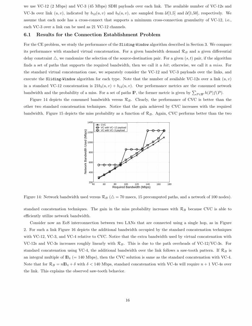
Figure 14 depicts the consumed bandwidth versus RB . Clearly, the performance of CVC is better than the

other two standard concatenation techniques. Notice that the gain achieved by CVC increases with the required

bandwidth. Figure 15 depicts the miss probability as a function of RB . Again, CVC performs better than the two

40 60 80 100 120 140 160 180200

400

600

800

1000

1200

1400

Required Bandwidth (Mbps)

Net

wor

k B

andw

idth

Use

d (M

bps)

CVCVC with VC−12 payloadVC with VC−3 payload

Figure 14: Network bandwidth used versus RB (△ = 70 msecs, 15 precomputed paths, and a network of 100 nodes).

standard concatenation techniques. The gain in the miss probability increases with RB because CVC is able to

efficiently utilize network bandwidth.

Consider now an EoS interconnection between two LANs that are connected using a single hop, as in Figure

2. For such a link Figure 16 depicts the additional bandwidth occupied by the standard concatenation techniques

with VC-12, VC-3, and VC-4 relative to CVC. Notice that the extra bandwidth used by virtual concatenation with

VC-12s and VC-3s increases roughly linearly with RB . This is due to the path overheads of VC-12/VC-3s. For

standard concatenation using VC-4, the additional bandwidth over the link follows a saw-tooth pattern. If RB is

an integral multiple of IB4 (= 140 Mbps), then the CVC solution is same as the standard concatenation with VC-4.

Note that for RB = nIB4 + δ with δ < 140 Mbps, standard concatenation with VC-4s will require n + 1 VC-4s over

the link. This explains the observed saw-tooth behavior.

16

40 60 80 100 120 140 1600

0.1

0.2

0.3

0.4

0.5

0.6

0.7

0.8

Required Bandwidth (Mbps)

Mis

s P

roba

bilit

y

CVCVC with VC−12 payloadVC with VC−3 payload

Figure 15: Miss probability versus RB (△ = 70 msecs, 15 precomputed paths, and a network of 100 nodes).

0 1000 2000 3000 4000 50000

100

200

300

400

500

600

700

Required Bandwidth (Mbps)

Add

ition

al O

ccup

ied

Link

Ban

dwid

th (

Mbp

s)

VC with VC−12 payloadVC with VC−3 payloadVC with VC−4 payload

Figure 16: Additional bandwidth over CVC that is required by standard concatenation with VC-12, VC-3, and VC-4.

17

6.2 Results for the Connection Upgrade Problem

For the CU problem, we study the performance of the Upgrade algorithm proposed in Section 4. For a given

simulation run, the values of C1 and C2 fall into one of the following three cases:

1. The delay of the shortest path between s and t w.r.t. w(., .) is greater than C2. In this case, there is no feasible

solution to the problem.

2. The delay of the shortest path between s and t w.r.t. w(., .) is less than C2 but greater than C1.

3. The delay of the shortest path between s and t w.r.t. w(., .) is less than C1.

Case 2 can be obtained from Case 3 by re-adjusting C1 (= W (P ∗)) and △ (= C2−W (P ∗)), where P ∗ is the shortest

path between s and t w.r.t. w(., .). Case 3 is nontrivial and is the one considered in our simulations. Accordingly, C1

and C2 are generated such that they are always greater than the length of the shortest path between s and t w.r.t.

w(., .). Specifically, we let C1 = W (P∗) + A + U [0, 50] and C2 = C1 + △, where A is a positive constant.

Figure 17 compares the Upgrade algorithm with the standard virtual concatenation (VC-12 and VC-3) in terms

of required network bandwidth by varying RB . The performance of CVC is better than the other two concatenation

techniques. The performance gain increases with RB .

50 60 70 80 90 100400

500

600

700

800

900

1000

1100

1200

Required Bandwidth (Mbps)

Net

wor

k B

andw

idth

Use

d (M

bps)

CVCVC with VC−12 payloadVC with VC−3 payload

Figure 17: Network bandwidth used versus RB (△ = 70 msecs, A = 50 msecs, 15 precomputed paths, and a networkof 100 nodes).

In Figure 18, we compare the performance in terms of the miss probability.

6.3 Result for Path Computation under Imprecise Network State Information

For a given topology, each link (u, v) is assigned a random delay w(u, v). We assume that w(u, v) is normally

distributed with mean µd(u, v) and variance σ2d(u, v). To produce heterogeneous link delays, we also randomize the

selection of µd(u, v) and σ2d(u, v) by taking µd(u, v) ∼ U [10, 50] msecs and σ2

d(u, v) ∼ U [10, 50] msecs2. The true value

of the link delay (w∗(u, v)) is sampled from a Gaussian distribution with mean µd(u, v) and variance σ2d(u, v). This

w∗ is used to check if the path returned by the algorithm is feasible. We set C1 and C2 as in Section 6.2, where P ∗ is

now the shortest path between s and t w.r.t. w∗(., .). The available number of VC-n channels over a link bn(u, v) is

sampled from U [lbn(u, v), ubn(u, v)], where we take lb3(., .) = 2, lb12(., .) = 10, ub3(., .) = 10, and ub12(., .) = 50. The

exact value of the number of VC-n channels available over a link (b∗n(u, v)) is sampled from U [lbn(u, v), ubn(u, v)].

18

50 60 70 80 90 1000

0.1

0.2

0.3

0.4

0.5

0.6

0.7

0.8

Required Bandwidth (Mbps)

Mis

s P

roba

bilit

y

CVCVC with VC−12 payloadVC with VC−3 payload

Figure 18: Miss probability versus RB (△ = 70 msecs, A = 50 msecs, 15 precomputed paths, and a network of 100nodes).

Let W (Pr) be the weight of this path Pr that is returned by the Backward-Forward algorithm w.r.t. w∗(., .), and

let b∗ be the available bandwidth. If C1 ≤ W (Pr) ≤ C2 and if C3 ≤ b∗, then we count it as a hit.

40 60 80 100 120 140 1600.1

0.2

0.3

0.4

0.5

0.6

0.7

0.8

Required Bandwidth (Mbps)

Mis

s P

roba

bilit

y

CVCVC with VC−12 payloadVC with VC−3 payload

Figure 19: Miss probability vs. RB for path selection under imprecise information (△ = 70 msecs, A = 30 msecs,and a network of 100 nodes).

In Figure 19, we depict the miss probability for a connection request versus RB . As shown in the figure, CVC

performs better than the other two concatenation techniques. Figure 20 shows the average number of iterations

needed to find a feasible path when no limit is imposed on K. Clearly, CVC incurs less computational time than the

two concatenation techniques considered.

7. Conclusions and Summary

In this paper, we introduced the general structure of cross-virtual concatenation (CVC) for EoS circuits. We proposed

a simple implementation of CVC that involves an upgrade at the end nodes and that reuses the existing SDH

overhead. We demonstrated the bandwidth gain of CVC over standard virtual concatenation. The algorithmic

problems associated with connection establishment and connection upgrade were studied. For the establishment of

a new EoS connection, we modeled the problem as a flow-maximization problem. An ILP solution as well as an

19

40 60 80 100 120 140 1601.5

2

2.5

3

3.5

4

4.5

5

5.5

6

Required Bandwidth (Mbps)

Ave

rage

Iter

atio

ns R

equi

red

CVCVC with VC−12 payloadVC with VC−3 payload

Figure 20: Number of iterations needed versus connection bandwidth (△ = 70 msecs, A = 30 msecs, and a networkof 100 nodes).

algorithm based on the sliding-window approach were proposed. For the connection upgrade problem, we modeled it

as a flow-maximization problem where the delay of each path in the solution set is required to satisfy the differential

delay constraint of the existing members of the VCG. We proposed an efficient algorithm called Upgrade for solving

this problem. We also considered the problem of path selection when the network state information is imprecisely

available at the time of path selection. Extensive simulations were conducted to show the effectiveness of employing

CVC for EoS systems. We contrasted the performance of CVC with the standard virtual concatenation in terms of

the miss probability and consumed network bandwidth. The results show that CVC harvests the SDH bandwidth

more efficiently, provides greater flexibility in terms of path selection, and reduces the miss probability for connection

establishment.

Acknowledgements: This work was supported by NSF under grants ANI-0095626, ANI-0313234, and ANI-0325979.

Any opinions, findings, conclusions, and recommendations expressed in this material are those of the authors and

do not necessarily reflect the views of NSF. An abridged version of this paper was presented at the IFIP Networking

Conference, Coimbra, Portugal, May 15-19, 2006.

References

[1] ANSI T1.105-2001, “Synchronous optical network (SONET): Basic description including multiplexing structure,

rates and formats,” 2001.

[2] ITU-T Standard G.707, “Network node interface for the synchronous digital hierarchy,” 2000.

[3] S. Acharya, B. Gupta, P. Risbood, and A. Srivastava, “PESO: Low overhead protection for Ethernet over

SONET transport,” Proceedings of the IEEE INFOCOM Conference, vol. 1, pp. 175–185, Mar. 2004, Hong

Kong.

[4] V. Ramamurti, J. Siwko, G. Young, and M. Pepe, “Initial implementations of point-to-point Ethernet over

SONET/SDH transport,” IEEE Communications Magazine, vol. 42, no. 3, pp. 64–70, 2004.

[5] R. Santitoro, “Metro Ethernet Services - a technical overview,” http://www.metroethernetforum.org/metro-

ethernet-services.pdf, 2003.

[6] ITU-T Standard G.7042, “Link capacity adjustment scheme for virtually concatenated signals,” 2001.

20

[7] A. Srivastava, S. Acharya, M. Alicherry, B. Gupta, and P. Risbood, “Differential delay aware routing for

Ethernet over SONET/SDH,” Proceedings of the IEEE INFOCOM Conference, vol. 2, pp. 1117–1127, Mar.

2005, Miami.

[8] Satyajeet Ahuja, Marwan Krunz, and Turgay Korkmaz, “Optimal path selection for minimizing the differential

delay in Ethernet over SONET,” Computer Networks Journal, vol. 50, pp. 2349–2363, Sept. 2006.

[9] S. Stanley and D. Huff, “GFP chips: Making SONET/SDH systems safe for Ethernet,” LightReading Webinar

Id=26778, http://www.lightreading.com, Feb. 2004.

[10] ITU-T Standard G.7041, “Generic Framing Procedure,” Feb. 2003.

[11] R. Ahuja, T. Magnanti, and J. Orlin, Network flows: Theory, Algorithm, and Applications, Prentice Hall Inc.,

1993.

[12] E. Chong, S. Maddila, and S. Morley, “On finding single-source single-destination k shortest paths,” Proceedings

of the Seventh International Conference on Computing and Information (ICCI ’95), pp. 40–47, July 1995,

Peterborough, Ontario, Canada.

[13] Michael R. Garey and David S. Johnson, Computers and Intractability: A Guide to the Theory of NP-

Completeness, W. H. Freeman, 2000.

[14] T. Korkmaz and M. Krunz, “Bandwidth-delay constrained path selection under inaccurate state information,”

IEEE/ACM Transactions on Networking, vol. 11, no. 3, pp. 384–398, June 2003.

[15] D. H. Lorenz and A. Orda, “QoS routing in networks with uncertain parameters,” IEEE/ACM Transactions

on Networking, vol. 6, no. 6, pp. 768 –778, Dec. 1998.

[16] A. Shaikh, J. Rexford, and K. G. Shin, “Evaluating the impact of stale link state on quality-of-service routing,”

IEEE/ACM Transactions on Networking, vol. 9, no. 2, pp. 162–176, Apr. 2001.

[17] M. Faloutsos, P. Faloutsos, and C. Faloutsos, “Power-laws of the Internet topology,” Proceedings of the ACM

SIGCOMM Conference, vol. 29, no. 4, pp. 251–262, Sept. 1999, Cambridge, Massachusetts, USA.

[18] BRITE, “Boston university representative Internet topology generator,” http://www.cs.bu.edu/brite/.

21